The decomposition of forecast in seasonal arima models

Journal 01 Forecasting, Vol. 14, 565-583 (1995)

The Decomposition of Forecast in Seasonal ARIMA Models

ANTONI ESPASA ANO DANIEL PEÑA Universidad Carlos 111 de Madrid, Spain

ABSTRACT

This paper presents a procedure to break down the forecast function of a seasonal ARIMA model in terms of its permanent and transitory components. Both depend on the initial values at the forecast origin, but their structures are fixed and independent of this origino The permanent component is an estimate of the long-run projection of the corresponding economic variable and the transitory element describes the approach towards the permanent one. Within the permanent component a distinction is made between the factors that depend on the initial conditions of the system and those that are deterministic. The procedure is compared to other methods presented in the literature and illustrated in an example.

KEY WORDS forecast function; long-term growth; seasonal components; trends; unit roots

INTRODUCTION

A disadvantage frequentIy attributed to ARIMA models is the difficu1ty in interpreting them in terms of the classical trend, seasonal, and irregular components (Chatfield, 1977; Harvey and Todd, 1983). A1though it is well known (Box and Jenkins, 1976) that the forecast function of a seasonal multiplicative ARIMA model can be represented as a combination of an adaptative trend and a seasonal component, until the work of Box et al. (1987) no simple, direct procedures had been developed for determining these components. These authors use the eventual forecast function together with signal extraction theory to perform a breakdown of the series into its components and they apply it to the IMA model (1.1) x (1.1), commonly known as the airline model.

In this work these ideas are generalized to obtain a breakdown of the forecast function into a permanent term, which is produced by the model's non-stationary operators, and a transitory term, which is produced by the stationary operators. AIso, in seasonal series the permanent term can be easily broken down into trend and seasonal components, and the transitory term can be also be decomposed into a seasonal and a non-seasonal termo Sorne of the results presented in this paper appeared in a more preliminary form in Spanish in Peña (1989) and Espasa and Peña (1990). This paper generalizes these results and provides a more precise economic interpretation of the forecasting function for economic variables.

In the application of time-series analysis to economic data, the decomposition of a series into components (such as trend and a residual with cyclical stationary behaviour, or trend, seasonal, eee 0277-6693/951070565-19 Received January 1994 © 1995 by John Wiley & Sons, Ltd. Accepted January 1995

1

566 Journal 01 Forecasting Vol.l4, [ss. No. 7

and residual, etc.) has attracted the attention of many authors. The procedures that have been proposed can be broadly classified in two groups: (1) full-information decomposition and (2) conditional decompositions. Examples of the first procedures are Box et al. (1978), Burman (1980), Hillmer and Tiao (1982), BeU and Hillmer (1984), MaravaU (1987), MaravaU and Gomez (1992), Maravall and Pierce (1987), and Harvey (1981, 1984). In these procedures the whole sample information is used to estimate the components. To achieve a unique decomposition it is usuaUy assumed that the components are driven by different and independent processes. This hypothesis is useful and has great advantages, but its economic foundation is not clear, because it could be expected that certain innovations entering into the system would alter at the same time the evolutions of aU the components.

The conditional decompositions obtain, at each moment t, the components of a time series conditional to the sample information up to t, or sorne previous moment in time. Examples of these decompositions are Box et al. (1987), Beveridge and Nelson (1981), and Watson (1986). These procedures can be used in a contemporaneous way for estimating at each t the different components of the series, like Beveridge and Nelson (1981), or for decomposing the future. The contemporaneous application of the conditional procedures for the breakdown of the present value implies that with information until time t = T the components at t = 1, ... , Tare obtained with different information for each t. For instance, in the Beveridge and Nelson procedure the cyclical or transitory component c, is what was considered transitory at moment t and not what could considered as such at T. Under the latter assumption the cyclical component could be very different. The question is that to be conditional up to each moment t when one could use all the sample information does not seem very useful.

For the future, the conditional decomposition is the on1y possible one and, as we will attempt to prove in this paper, it provides a useful tool for understanding the forecast function. As non­stationary time series do not have a stable and defined absolute mean, the forecast for a long horizon does not collapse to an absolute mean as is the case for stationary series. In this context it seems use fuI to decompose the forecast into one transitory part, which sooner or later collapses to zero, and a permanent part, which never approaches zero. This approach is useful in analysing how the innovations which arrive to a system will propagate in the future in a permanent factor-usually of a quasi-linear type-and in a stationary one. In addition, for series which show a maintained growth with time but with their levels oscillating considerably around an hypothetical trend, it could be of interest to analyse the change in the slope that occurs in the permanent component of the updated forecast each time there is an innovation. The forecasting robustness showed by ARIMA models is due to the fact that these models, with constant parameters, imply forecasting functions with a linear permanent component whose parameters change with time.

Also, the decomposition suggested in this paper has sorne important advantages: it makes interpretation of the model easier; it is a useful diagnostic tool for identifying interventions which may affect the trend or seasonal parts (see Peña, 1989) and it offers a means of comparison between ARIMA model~ and models in state space representation either in their Bayesian form (Harrison and Stevens, 1976) or in their structural one (Harvey and Todd, 1983).

This work is structured as foUows: the next section defines the permanent and transitory terms of the prediction function of an ARIMA model and describes the breakdown of the permanent term into trend and seasonal components. The third section discusses an economic interpretation of the components of the forecast function. The fourth section shows how these components are determined on the basis of the ARIMA model's prediction by solving a system of linear equations. The fifth section compares our approach with other decompositions suggested in the econometric literature, as those of Beveridge and Nelson (1983) and Watson (1986). The final section presents sorne applications.

2

Antoni Espasa and Daniel Peña Seasonal ARIMA Models 567

2. SEASONAL MODELS, THEIR FORECAST FUNCTIONS AND THEIR COMPONENTS

Seasonal models and their forecast functions A linear stationary stochastic process without deterministic components can be represented according to Wold's theorem by:

x, = 'JI(L)a, (1)

where 'JI(L) = 1 + 'JI,L + 'JI2L2 + .,. is an infinite convergent polynomial in the lag operator L,

and a, is generated by a white-noise stochastic process. Approximating this polynomial by means of a ratio of two finite-order polynomials the ARMA representation is obtained;

ifJ(L)X,= O(L)a, (2)

where 'JI(L) = [ifJ(L)r'O(L) and the operator ifJ(L) has all the roots outside the unit circ1e so that the process is stationary. Usually it is also assumed, as we do in this paper, that the roots of O(L) are also outside the unit circ1e and then the process is invertible. For seasonal processes, Box and Jenkins (1976) simplify equation (2) by factorizing the polynomials into two operators, one on L and another on U, where s is the seasonal periodo

Many economic time series do not have a stable and defined mean and need to be transformed before Wold's theorem can be app1ied to them. In the Box-Jenkins tradition, experience shows that by differencing, regular and seasonally, one very often obtains a transformed series which could be considered generated by model (2). This means that if X, is the series of interest, one may end up applying Wold's theorem to W, = MsX, - ,u(t), where ~ = 1 - L is the regular difference operator, ~s = 1 - U is the seasonal difference operator, and ,u is a time polynomial of finite order (m - 1). Then the resulting model for X, is

(3)

which is known as the seasonal multiplicative ARIMA model. When m equals one the time polynomial is a constant that will be denoted by ,u. In this paper we deal only with integer values for d. Calling CPr(L) = ifJp(L)c'bp(U2~d~s; r=p+d+s(l +P); O*m(L) = O/L)8 Q (U); p=q+sQ; c=~p(L)c'bp(U),u(h) and X,(h) the prediction of X'+h from the origin 1, we see that this prediction is given by:

r v

X,(h) = I cp,X,(h - i) + I e/a,+h_j + e (4)

where the predictions X,(h - i) coincide with the values observed when the horizon is negative, and the disturbances a,+h_j are zero if h > j and identical to the estimated values if j?!- h.

For h> p the MA part of the model will have no direct effect on prediction. Consequently, for a relatively distant time horizon the so-called eventual forecast function is obtained:

X,(h) = cp,X,(h - 1) + ... + cp,x,(h - r) + e (5)

The number of differences in equation (3) is 0= d + 1 and this shows that, even in the case of m = 1, the solution of equation (5) tends to infinity if o is equal to or greater than two or if o is one and ,u is different from zero. This indicates that the unit root factors induce long-term projections which do not seem acceptable for economic variables. The question is that the unit value for one of the roots of cp,.(L) implies a discontinuity from values just over one and with the sample sizes available it is not possible to distinguish between both alternatives which have almost identical implications for short- and medium­term projections. Therefore, in practice, the unit root assumption does not cause a serious

3

568 Journal 01 Forecasling Vol. 14, [ss. No. 7

problem, but it certainly cannot be taken to represent the very long-term projection of economic variables. This problem will be better illustrated in the next section once the decomposition of the solution of equation (5) had been discussed, but it must be pointed out that the structure of Xt +h as h -+ 00 cannot be derived from finite samples. Nevertheless any dynamic model which could be specified to explain the generation of data in a sample will have in it a particular structure for long-term projection. The analyst, at most, could discriminate if one structure is preferable to another to explain data, and in this respect the unit root assumption has done well.

The solution of the difference equation (5) provides the structure of the forecast function, as given by the following theorem.

Theorem. The general solution to the homogenous difference equation

A (L)Zt = O, (6)

where A(L) = 1 + a1L + ... + a,,[} is a finite polynomial in the lag operator which can be factorized as:

A(L) = P(L)Q(L) (7)

where the polynomials P(L) and Q(L) are prime (they do not have common roots), can always be written as:

Zt=Pt+qt (8)

where the sequences Pt and qt are the solutions corresponding to each prime polynomial, that is, they verify:

P(L)pt = Q(L)qt = O

The proof of this theorem is given in the Appendix.

(9)

To apply this theorem, let us note that the eventual forecast function can be written, for h > p:

fj>*(L)(fldflsXt(h) - /-l(h» = O (10)

where fj>*(L) = fj>p(L)«I>p(L') and the L operator acts on the index h, and 1, the origin of the prediction, is fixed. The stationary operator fj> * (L) has aH the roots outside the unit circle, and the operator (1 - LS) can be written:

(1 - U) = (1- L)S(L) (11)

where S(L) = (1 + L + ... + U-1). This operator has s - 1 roots, aH of them in the unit circle. If s is even, these s - 1 roots include L = -1 and other s - 2 complex conjugated roots with a unit module and distributed symmetricaHy in the unit circle. ConsequentIy, the stationary operators fj> * (L) and the non-stationary ones I:!.'d/is have no root in common, and the eventual forecast function can always be broken down into two components:

Xt(h) = Pt(h) + lt(h)

where

(1) pt(h) is the permanent component of the long-term forecast, which is determined only by the non-stationary part of the model and is the solution to:

/id/isPt(h) = /-l(h) (12)

4

Antoni Espasa and Daniel Peña Seasonal ARIMA Models 569

(2) t,(h) is the transitory component, which is determined by the stationary autoregressive operator. This component defines the approach towards the permanent component and is given by:

(13)

In the next section we study the form of these components on the basis of the ARIMA model and the following section shows how to calculate them.

The transitory component The transitory component of the eventual forecast functíon is the solution to equation (13). The general solution to this homogenous difference equation, assuming that the n = p + Ps roots of the polynomialljJ*(L) are different, is

t,(h) = b\r)G~ + ... + b~r)G~ (14)

where Gil, ... , G;I are the roots of the autoregressive polynomial and b}') are coefficients depending upon the origin of the prediction. Since the operator ljJ * (L) is stationary, the terms Gj

will be all in module les s than one. ConsequentIy,

lim t,(h) = 'i:.bJ) lim G/ = O (15) h~oo h~oo

and the transitory component will be zero in the long termo This same reasoning is valid when a identical roots exist, since in that case the term associated with a equal roots, G, will be:

[b\')+b~r)h+ .. ·+b~)ha-I]Gh (16)

which will tend once more to zero when h ~ 00 if I G I < 1. ConsequentIy, the transitory component specifies how the transition towards the permanent component is produced and it disappears for high prediction horizons. When the roots are real equation (14) consists of a mixture of damped exponentials, if two roots are complex they produce a damped sine wave.

The transitory component can be decomposed into a seasonal and a non-seasonal part by using the roots of the operators ljJp(L) and 4>p(U). For monthly data s= 12, and a seasonal autoregressive polynomial of the type (1 - 4>IL 12) has twelve roots, ten of them complex that will produce harmonic functions and they can be interpreted as short-term cyc1es within the year. The real negative root will produce a cyc1e of two months.

The permanent component By using the factorisation (11) the permanent component of the long-term forecast function (12) can be written as follows:

(17)

According to the theorem in the previous subsection the solution to this equation can, in tum, be broken down into two terms associated with the prime polynomials ~d+1 and S(L). The first, which we will call the trend component, T" will be the solution of:

~d+IT,(h) = e (18)

where c=p,(h)· [s(L)r l, the second, which we will call the seasonal component, E" is the

solution of:

(19)

5

570 Journal 01 Forecasting Vol. 14, ¡ss. No. 7

It can be immediately checked that these components satisfy equation (17). In the next subsection their properties are analysed.

The trend component The trend component of the model is the solution of equation (18) which can be written:

Tf(h) = c~t) + c\tlh + ... + C~tlhd + C~hd+l + c;hd+2 + ... + c*mhd+m (20)

This trend is. in the general case. a polynomial of degree d + m and has d + 1 coefficients c~tl • ... , c~t) varying with the origin of the prediction and m coefficients c ~, ... , c ~ which are fixed. For m = 1.

ct = fl sed + 1)!

If there are no seasonal differences the order of the polynomial is max [O. (d - 1)] if ¡,t = O and (d + m - 1). whereas if there is a seasonal difference the trend polynomial is of degree d if ¡,t(t) = O and (d + m) otherwise.

The seasonal component The seasonal component of the modelo the solution of equation (19). is a function of period s with values summing zero each s lag. We will call

Shf) = Ef(h). h = 1 •...• s

the s coefficients of equation (19). which are the seasonal coefficients of the forecast function. It should be noted that the seasonal coefficients must verify the restriction

so we have only (s - 1) unknown coefficients to be determined by the initial conditions. The superscript t in the seasonal coefficients indicates that these coefficients vary with the origin of the prediction and are updated as new data arrive.

The long-term forecast function As we have seen. in the long term the transitory component of the eventual forecast function will be zero and only the permanent component remains. That is. for a very large h

Xf(h) = Tf(h) + Ef(h)

where Tf(h) is a polynomial trend and Ef(h) is the seasonal component which is repeated evely s periodo

ECONOMIC INTERPRET ATION OF THE COMPONENTS OF THE UNIV ARIA TE FORECAST FUNCTION

In this section we attempt to analyse the type of information provided by the forecast function corresponding to an economic variable. We have followed Espasa and Cancelo (1993. Section 2.8), but here we give a more precise economic interpretation of the forecasting function. The predictions described in the previous section for different values of h are the expectations at

6

Antoni Espasa and Daniel Peña Seasonal ARIMA Models 571

moment t on the values of the variable in t + 1, t + 2, ... , conditioned to past values of the series. From now on we make the standard assumption in linear system analysis that these conditional expectations always exist.

If the parameters of the ARIMA model are known, the value X'+h can be broken down as following way:

X'+h =X,(h) + e'+h

where e'+h denotes the prediction error which is equal to

(21)

(22)

Equation (21) divides the observed value X'+h into two independent parts (1) X,(h), the expectation for X'+h which we have at moment t; and (2) e'+h' the effect of the surprises which occurred between t + 1 and t + h, which is obtained as a weighted sum of the corresponding innovations.

When h tends to infinity, the forecast function indicates the long-term value to which the variable would tend if in the future the stochastic innovations or disturbances which affect the system were zero. Therefore, giving high values to h the forecast function describes the conditional long-term projection of the economic variable in question. Thus, in the case of a variable which after differencing once is stationary with zero mean, the limit of the forecast function is a constant and we will conclude that conditional on the values of the system at the forecasting origin t, the projection of the variable tends to a stable value, b&t). In (t + k) the system would have suffered from innovations a,+ 1, ••• , a'+b the conditions of the system would have changed and at this origin (t + k) the projection of the variable will tend to a stable future value, but a different one, bg+k ). In fact, [bg+ k ) - bg)] measures the long-term effect of the innovations arrived to the system between t and t + k. In all other cases of non-stationary mean level, the limiting forecasting function of model (3) does not tend to a stable value but evolves according to a time polynomial.

In conclusion, on the one hand, the forecast function enables us to quantify the different term univariate expectations for a particular phenomenon; on the other, the trend of the forecast function describes the long-term projection path towards which this phenomenon is moving at each moment t.

In adding comments to the concept of integrated variables defined in Engle and Granger (1987) we will say that a variable generated by an ARIMA model is integrated of order (o, m) if for stationarity it needs to be differentiated o times and the differenced transformation has a mathematical expectation given by a time polynomial of order (m - 1). If in the previous case the mathematical expectation of the differenced transformation is a constant, we see that such expectation follows a polynomial of order O = m - 1. In this case it is important to distinguish the situation in which the expectation is not zero from the one in which it is. In the former case, and consequentIy with our definition of m, we would say that m equals one and the long-term projection will be given by a polynomial of order (o + m - 1). But when the expectations is not only constant but also zero, then we will say that m = O and the long-term projection will be given by a polynomial of the order (o + m - 1) if O;¡¡, 1 and of order zero if 0=0. For this convention for the values of m and from what has been seen in the previous section, we note that the order of integration fully describes the polynomial structure of the trend of the forecast function, which will be of the order max(O, o + m - 1). The trend is purely stochastic in the sense that all its coefficients are determined by the initial conditions of the system, if m is zero, and it is mainly deterministic if mis different from zero.

This definition of integration makes explicit the presence or otherwise of a constant or a time

7

572 Journal 01 Forecasting Vol. 14, [ss. No. 7

polynomial in the differenced series due to the importance which, as we shaH see, they have. If o + m adds to zero or one the forecasting function tends to a constant, the value of which will be purely deterministic if o is zero, or it will be determined by the initial conditions if o is one. If o + m adds to more than one, the forecasting function does not tend to a stable value, but evolves according to a polynomial structure that, in the long term, will depend on the coefficient corresponding to the greatest power, since compared to it, aH other powers have a negligible contribution. Now, at least this coefficient will be deterministic if m is equal to or greater than one, in which case the long-term projection of the variable could also be considered to be deterministic. This means that the factor which contributes most to this path is not altered by changes in the conditions of the system, and therefore if that was the case, the development of an economic theory to explain in this situation the long-term path of a variable (Le. consumption) in terms of another (e.g. income) would not be of much help. On the contrary, if m is zero aH the parameters of the trend of the forecast function depend on the initial conditions of the system. In such cases the long-term projection is determined by a time polynomial of the order (B - 1), but the parameters of this polynomial change as new disturbances reach the system.

To complete the description of the long-term projection of an economic variable we must specify the magnitude of the uncertainty we have about it. This uncertainty is expressed by et +h

in equation (21) when h tends to infinity. If the process is stationary, in which case 0=0, the polynomial 'IjJ(h) which enters the definition (22) of et+h is convergent and the variance of et+h when h tends to infinity is finite. This result is true even when bearing in mind the uncertainty associated with the estimation of the parameters (see Box and Jenkins, (1976, Appendix A7.3). In such a case, we say that the uncertainty regarding the future, however far off it may be, is limited. If o is not zero, 'IjJ(h) does not converge, and the variance of et+h tends to infinity with h, so we can say that uncertainty regarding the future is not bounded.

Note that in a structural economic model (SEM) where exogenous variables are generated by non-stationary ARIMA models, long-term predictions are also generated on the endogenous variables with non-bounded uncertainty. The difference with respect to the ARIMA predictions can be found simply in the fact that the uncertainty may tend to infinity slower and with a greater delay.

The characteristic of the long-term projections derived from the ARIMA models with the most common values for o and m are shown in Table 1. An ARIMA model with (o + m = 2) implies that in the long term, projection of the corresponding variable tends to infinity. Such a characteristic may be considered as unacceptable in economics, but note that if m = O simply substituting one of the positive unit roots included in the differentiations by (0.999) -1 will be sufficient for the law of the long-term projection to become a constant. However, the way in which this constant value would be achieved depends on the transitory component of the prediction function It(O), defined in equation (13). As this component will in this case have a term bIt) (0.999)h it will not be canceHed out in the medium term and, in practice, this will not be distinguished from the first mentioned in which (o + m) equaHed two.

Consider the foHowing example in which we have: (1) an eventual forecasting function with two unit roots and (2) another one with one unit root and a second root (0.999) -l. In the latter case the long-term projection will be given by

(23)

In equation (23) when h tends to infinity Xt +h tends to bg) (permanent component) but the transitory component (- bIt) . 0.999 h

) indicates that the value bg) will be attained subtracting the factor b l ·0.999\ which decreases with h but does not cancel for moderate values of h. Since

8

Antoni Espasa and Daniel Peña Seasonal ARIMA Models 573

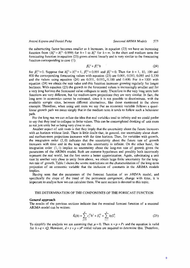
the substructing factor becomes smaller as h increases, in equation (23) we have an increasing function from (b~t) - bIt) . 0.999) for h = 1 to bót) for h = oo. In the short and medium term the forecasting function in equation (23) grows almost 1inearly and is very similar to the forecasting function corresponding to case (1):

f3gl + f3\t) h (24)

for f31t\> O. Suppose that b~t) = bIt) = 1, f3¡tl = 0.001 and f3gl = O. Then for h = 1, 10, 100 and 400 the corresponding forecasting values with equation (23) are 0.001, 0.010, 0.095 and 0.330 and the values using equation (24) are 0.001, 0.010,.0.100 and 0.400. For h = 1000 with equation (24) we obtain the unit value and this function increases growing regularly for longer horizons. With equation (23) the growth in the forecasted va1ues is increasingly smaller and for a very long horizon the forecasted value collapses to unity. Therefore in the very long term both functions are very different, but for medium-term projections they are very similar. In fact, the long term in economics cannot be estimated, since it is not possible to discriminate, with the available sample sizes, between different altematives, like those mentioned in the aboye example. Therefore, when using unit roots we say that an economic variable follows a quasi­linear growth path we mean simply that in the medium term it tends to follow such a behaviour path.

For the long run we can refute the idea that real variables tend to infinity and we could prefer to say that they tend to collapse to finite values. This can be contemplated thinking of unit roots as not just unity but as being very close to one.

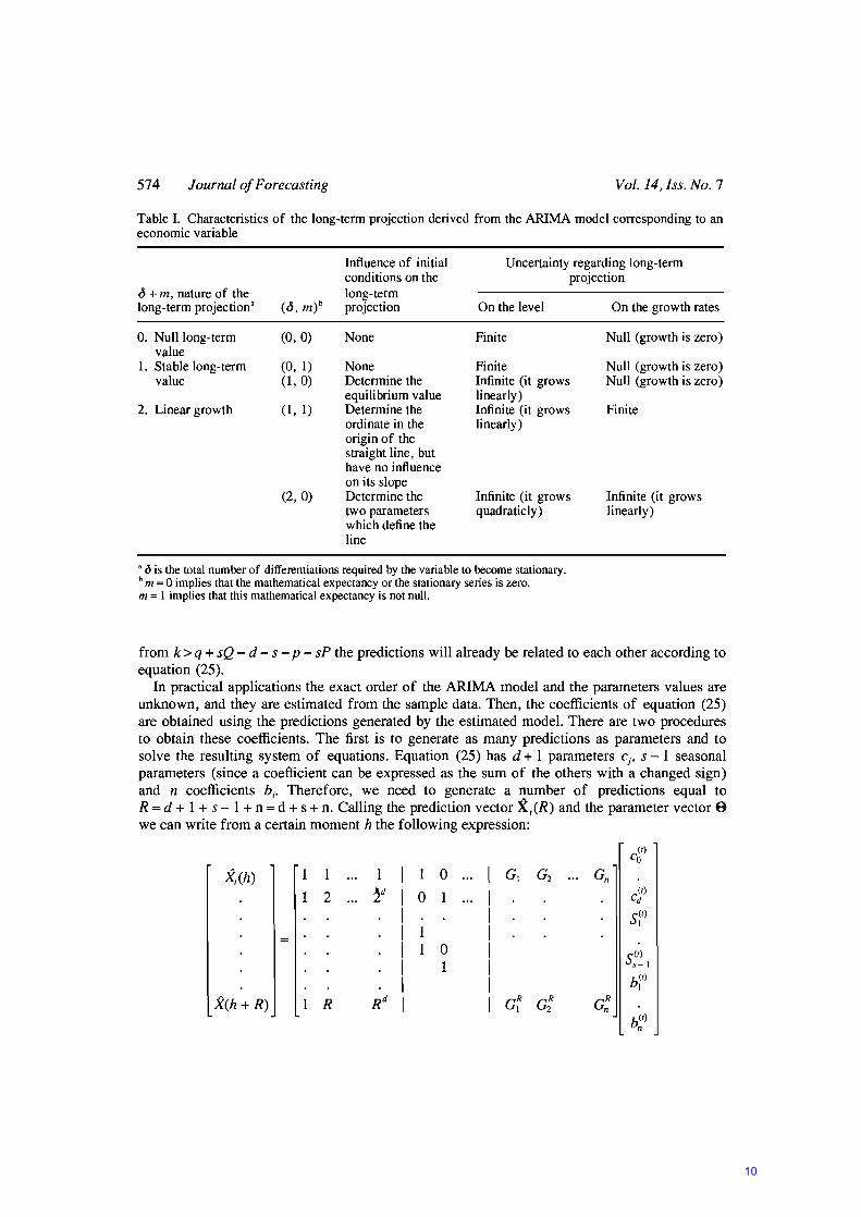
Another aspect of unit roots is that they imply that the uncertainty about the future increases with an horizon without limit. There is líttle doubt that, in general, our uncertainty about short­and medium-term projections increases with the time horizon. Thus, for variables with growth, the integration order (2, O) indicates that the uncertainty about the future rate of growth increases with time and in the long run this uncertainty is infinite. On the other hand, the integration order (1,1) implies no uncertainty about the long-run rate of growth given the parameters of the ARIMA model. Both are extreme hypotheses and possibly both incorrecdy represent the real world, but the first seems a better approximation. Again, substituting a unit root by another very close to unity from aboye, we obtain large finite uncertainty for the long­run rate of growth. Table I shows the severe restrictions on the characterization of the long-term projection of an economic variable that the inclusion of constants in the ARIMA models implies.

Having seen that the parameters of the forecast function of an ARIMA model, and specifically the slope of the trend of the permanent component, change with time, it is important to analyse how we can calculate them. The next section is devoted to this topic.

THE DETERMINATION OF THE COMPONENTS OF THE FORECAST FUNCTION

General approach The results of the previous sections indicate that the eventual forecast function of a seasonal ARIMA model can be written:

d n

Xt(h) = I cjtlh j + S~l + I b;G~ (25) j=O ;= 1

To simplify the analysis we are assuming that ¡,t = O. Then n = p + Ps and the equation is valid for h > q + sQ. However, d + s + p + sP initial values are required to determine this. Therefore,

9

574 Journal 01 Foreeasting Vol. 14, ¡ss. No. 7

Table 1. Characteristics of the long-term projection derived from the ARIMA model corresponding to an economic variable

<5 + m, nature of the long-term projectiona (<5, m)b

O. Nulllong-term (O, O) value

l. Stable long-term (O, 1) value (1, O)

2. Linear growth (1, 1)

(2, O)

Influence of initial conditions on the long-term projection

None

None Determine the equilibrium value Determine the ordinate in the origin of the straight line, but have no influence on its slope Determine the two parameters which define the line

Uncertainty regarding long-term projection

On the leve!

Finite

Finite Infinite (it grows linearly) Infinite (it grows linearly)

Infinite (it grows quadraticly)

On the growth rates

Null (growth is zero)

Null (growth is zero) Null (growth is zero)

Finite

Infinite (it grows linearly)

a el is the total number of differentiations required by the variable to become stationary. b m = O implies that the mathematical expectancy or the stationary series is zero. m = 1 implies that this mathematical expectancy is not null.

from k> q + sQ - d - s - p - sP the predictions will already be related to each other according to equation (25).

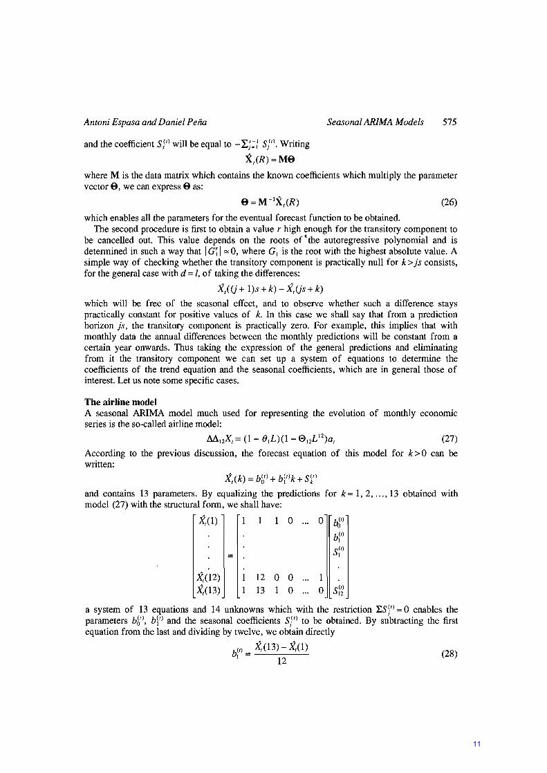
In practical applications the exact order of the ARIMA model and the parameters values are unknown, and they are estimated from the sample data. Then, the coefficients of equation (25) are obtained using the predictions generated by the estimated model. There are two procedures to obtain these coefficients. The first is to generate as many predictions as parameters and to solve the resulting system of equations. Equation (25) has d + 1 parameters ej , s - 1 seasonal parameters (since a coefficient can be expressed as the sum of the others with a changed sign) and n coefficients b¡. Therefore, we need to generate a number of predictions equal to R = d + 1 + s - 1 + n = d + s + n. Calling the prediction vector Xr(R) and the parameter vector 8 we can write from a certain moment h the following expression:

Xr(h)

X(h + R)

1 1

1 2

R

1 O O 1

O 1

Gn

GR n

(r) Ca

(r) ed

S~r)

S(r) s- 1

b~t)

b(r) n

10

Antoni Espasa and Daniel Peña

and the coefficient sIl) will be equal to - 'LJ:! Sr). Writing

X,(R)=Me

Seasonal ARIMA Models 575

where M is the data matrix which contains the known coefficients which multiply the parameter vector e, we can express e as:

8=M- 1X,(R) (26)

which enables all the parameters for the eventual forecast function to be obtained. The second procedure is first to obtain a value r high enough for the transitory component to

be cancelled out. This value depends on the roots of 'the autoregressive polynomial and is determined in such a way that I C; I '" O, where C I is the root with the highest absolute value. A simple way of checking whether the transitory component is practically null for k> js consists, for the general case with d = 1, of taking the differences:

X,(U+ l)s+k)-X,Us+k)

which will be free of the seasonal effect, and to observe whether such a difference stays practically constant for positive values of k. In this case we shall say that from a prediction horizon js, the transitory component is practically zero. For example, this implies that with monthly data the annual differences between the monthly predictions will be constant from a certain year onwards. Thus taking the expression of the general predictions and eliminating from it the transitory component we can set up a system of equations to determine the coefficients of the trend equation and the seasonal coefficients, which are in general those of interest. Let us note sorne specific cases.

The airline model A seasonal ARIMA model much used for representing the evolution of monthly economic series is the so-called airline model:

M I2X, = (1- OIL)(l - 9 12L 12)a, (27)

According to the previous discussion, the forecast equation of this model for k> O can be written:

X,(k) = bg) + blt)k + S~I)

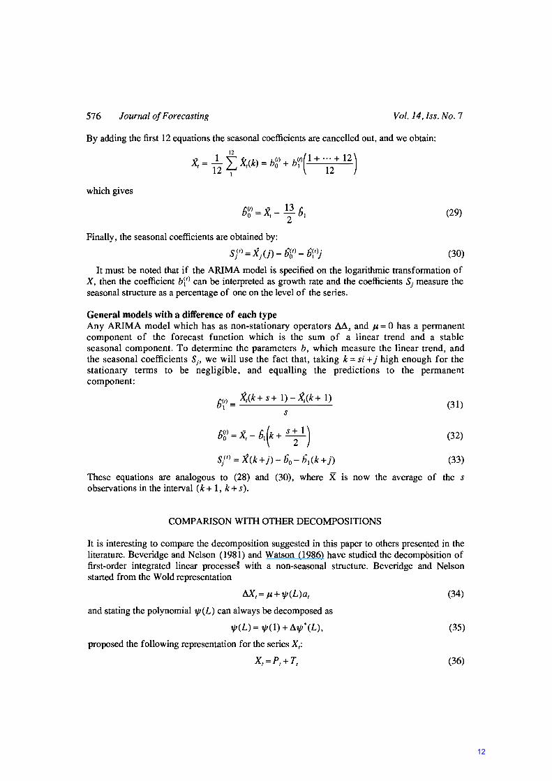
and contains 13 parameters. By equalizing the predictions for k = 1, 2, ... , l3 obtained with model (27) with the structural form, we shall have:

X,(l)

X,(12) X,(l3)

1

12 l3

1 O

O O O

oo. O b6r)

b;r)

sir)

1 O S(t)

12

a system of 13 equations and 14 unknowns which with the restriction 'LSjt) = O enables the parameters bg), bl') and the seasonal coefficients SF) to be obtained. By subtracting the first equation from the last and dividing by twelve, we obtain directly

(1) X,(13) - X,(l) bl = (28)

12

11

576 Journal 01 Forecasting Vol. 14, Iss. No. 7

By adding the first 12 equations the seasonal coefficients are cancelled out, and we obtain:

X = J... ~ X (k) = b(t) + b(t)(1 + ... + 12) t 12 L... t o I 12

I

which gives

(29)

Finally, the seasonal coefficients are obtained by:

SP) = X/j) - 6g) - 6\t)j (30)

lt must be noted that if the ARIMA model is specified on the logarithmic transformation of X, then the coefficient bIt) can be interpreted as growth rate and the coefficients Sj measure the seasonal structure as a percentage of one on the level of the series.

General models with a dift'erence of each type Any ARIMA model which has as non-stationary operators AAs and ¡,t = O has a permanent component of the forecast function which is the sum of a linear trend and a stable seasonal component. To determine the parameters b, which measure the linear trend, and the seasonal coefficients Sj' we will use the fact that, taking k = si + j high enough for the stationary terms to be negligible, and equalling the predictions to the permanent component:

S~) = Xt(k + s + 1) - Xt(k + 1)

s

sg) = Xt - SI (k + s ~ 1 )

st) = X(k+ j) - 60 - 61(k+ j)

(31)

(32)

(33)

These equations are analogous to (28) and (30), where X is now the average of the s observations in the interval (k + 1, k + s).

COMPARISON WITH OTHER DECOMPOSITIONS

It is interesting to compare the decomposition suggested in this paper to others presented in the literature. Beveridge and Nelson (1981) and Watson (1986) have studied the decompbsition of first-order integrated linear processd with a non-seasonal structure. Beveridge and Nelson started from the W old representation

Mt = ¡,t + tp(L)at

and stating the polynomialtp(L) can a:1ways be decomposed as

tp(L) = tp(1) + Atp*(L),

proposed the following representation for the series Xt:

Xt=Pt+Tt

(34)

(35)

(36)

12

Antoni Espasa and Daniel Peña

where

~

Pr = tp(1) I at-j + ¡,t j=o

T,= tp*(L)a,

For instance, suppose that tp(L) is a MA(1) process. Then, as

M, = ¡,t + (1 - OB)a,

the resúlting decomposition is:

and

Seasonal ARIMA Models 577

(37)

(38)

(39)

(40)

(41)

(42)

Thus, the permanent component is a random walk with drift and the transitory component a white-noise process. Watson (1986) used a similar approach for the permanent component (a random walk with drift) but followed a model-based approach for the transitory component allowing different degree of correlation between the innovation in the components.

The decomposition suggested in this paper differs from both in several aspects:

(1) It is a decomposition not of the series itself but of the forecast function. (2) It can be applied to any ARIMA model, seasonal or not, whereas the previous

decompositions applies only to non-seasonal first-order integrated ARIMA models. (3) It is unique, as proved in the theorem, whereas the previous decompositions are noto

For instance, the decomposition of the forecast function for model (39) is, for k> O:

X,(k) = Pt(k) + T,(k)

P,(k) = P(~ + ¡,tk

T,(k) = O

that is, it contains only a linear function with slope ¡,t.

AN APPLICATION TO SERIES OF THE SPANISH ECONOMY

In this section an estimate is made, for a certain sequence of months, of the trend growth rate derived from the forecast function of the following series of the Spanish economy: imports, exports and the consumer price index for services. The use of the above-mentioned rate in a relatively complete short-term analysis of an economic phenomenon is put forward and described in Espasa and Cancelo (1993, Chapter 6). Following their terminology, in a univariate ARIMA model, we will call inertia to the rate 01 growth 01 the trend 01 the lorecast lunction, which will be given by the parameter b¡ defined in equation (31), when the model is specified on the logarithmic transformation of the variable.

13

578 !oumal of Forecasting Vol. 14, Iss. No. 7

Regarding Spanish foreign trade on non-energy goods, the following univariate monthly models were built to explain imports (M) and exports (X):

M l2 ln Mt= M l2 AlMt+ (1- O.77L)(l- 0.72L I2 )at a=0.092

M l2 In Xt = M l2 AlXt + (1 - 0.83L)(1 - 0.72L I2 )at a= 0.117

(43)

(44)

in which AlM and AIX are particular intervention analyses which have no effect upon the slope of the forecast function. Therefore, henceforth we will ignore them.

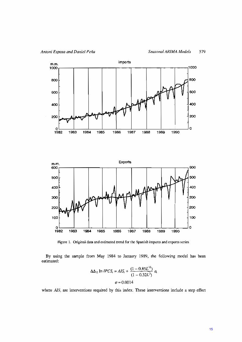
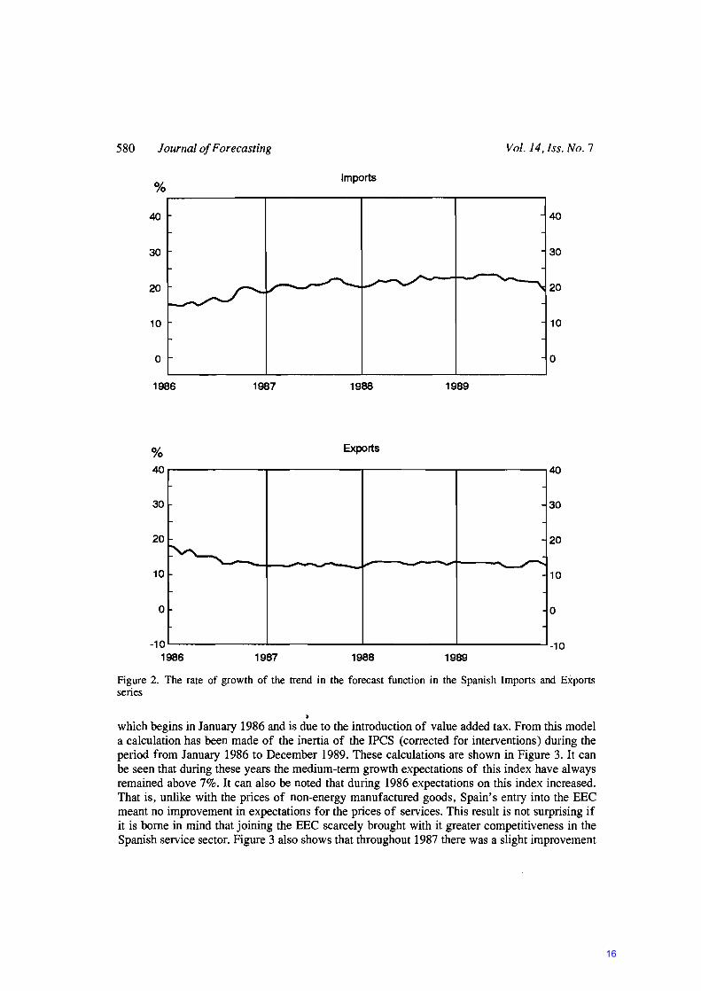
The original series with their corresponding trends are given in Figure 1 and the inertias are shown in Figure 2. The trends have been estimated using the X-ll-ARIMA procedure.

Figure 2 shows these inertias from January 1986, the month in which Spain joined the EEC, to December 1989. Thus, this figure illustrates what happened to Spanish overseas trade in nominal terms from that date. Obviously, on the basis of this description, no causal analysis can be made, since these models do not incorporate the determining variables of M and X that are responsible for the trend changes. Nevertheless, the mere description of these changes is in fact of interest in itself. However, it must be pointed out that the trend evolutions shown in Figure 2 refer to the sale and purchase of goods in nominal terms and, therefore, prices are also influencing these same trend movements.

We can deduce from Figure 2 that trend growth expectation in nominal imports increased systematical1y throughout 1986 and first three quarters of 1987. Then this expectation stabilized, with minor oscillations, at around 23% until the second half of 1989, when it started the decrease very slowly. As a result, a worsening (increasing) of perspectives for Spanish imports of around four percentage points has occurred during this periodo

With exports there was a movement from a growth expectation of 18% at the beginning of 1986 to an expectation of around 14% at the end of that year and during 1987. Since then expectations have remained fairly stable.

In conclusion, we can say that the perspectives for imports worsened (increased) progressively in 1986 and 1987, having a relatively stable evolution from that time until the second half of 1989, when an improvement occurred. As for expectations for exports, although they worsened (declined) during 1986, they maintained a fairly high level during the last three years of the sample considered. If the evolutions of imports and exports are compared in order to have a better understanding of the Spanish trade deficit at the end of 1989, a conclusion at that time was that given that the level of imports was higher than that of exports it was necessary at least for the growth rates expected in both series to equal each other fairly quickly. Also, insofar as expbrt growth could be considered as optimistic, given the level of world commercial activity and the relative level of Spanish prices compared to the rest of the world, to bring these rates together must require a significant reduction in import growth.

In the consumer price index for the Spanish economy the component measuring the prices of services, which we shall call IPCS, has been showing fairly uneven behaviour with regard to the component measuring the prices for non-energy manufactured goods. Both components make up the IPSEBENE, the consumer price index for services and non-energy manufactured goods, which represents 77.54% of the IPC, and it is an appropriate index on which to analyse underlying inflation or the inflationary trend.

14

Antoni Espasa and Daniel Peña Seasonal ARIMA Models

Imports m.m. 1000r-----r-----r---~----~----~------r_--~r_--~----~1000

O~----~--~----~----~----~----~----~--~~--~O 1982 1983 1984 1985 1986 1987 1988 1989 1990

Exports m.m. 600.-----~----~--~._--_,----~._----r_----r_--_.----~600

500 500

400 400

300 300

200 200

100 100

O~--~~--~----~----~----~----~----~--~ ____ ~O 1982 1983 1984 1985 1986 1987 1988 1989 1990

Figure 1. Original data and estimated trend for the Spanish imports and exports series

579

By using the sampIe from May 1984 to January 1989, the following modeI has been estimated:

M In IPeS = AIS + (l - O.85L 12) 12 , '(l _ O.32L3) a,

a=O.OO14

where AIS, are interventions required by this indexo These interventions include a step effect

15

580 Journal 01 Forecasting

%

40

30

20

10

o

1986

% 40

30

20

10

O

~

·10 1986

1987

1987

-

Vol. 14, ¡ss. No. 7

Imports

10

1988 1989

Exports

40

30

20

- ~ - - -10

O

-10 1988 1989

Figure 2. The rate of growth of the trend in the forecast function in the Spanish Imports and Exports series

• which begins in January 1986 and is due to the introduction of value added tax. From this model a calculation has been made of the inertia of the IPCS (corrected for interventions) during the period from January 1986 to December 1989. These calculations are shown in Figure 3. It can be seen that during these years the medium-term growth expectations of this index have always remained aboye 7%. It can also be noted that during 1986 expectations on this index increased. That is, unlike with the prices of non-energy manufactured goods, Spain's entry into the EEC meant no improvement in expectations for the prices of services. This result is not surprising if it is borne in mind that joining the EEC scarcely brought with it greater competitiveness in the Spanish service sector. Figure 3 also shows that throughout 1987 there was a slight improvement

16

Antoni Espasa and Daniel Peña Seasonal ARIMA Models 581

9.0 9.0

8.5 8.5

8.0 8.0

7.5 7.5

7.0 7.0

6.5 6.5

6.0 '"'-------....... ------"'-------...... -------' 6.0 1986 1987 1988 1989

Figure 3. The rate of growth of the trend in the forecast function in the Consumer Price Index for Services in Spain

(falI) in the IPCS inertia, which disappeared completely in 1988, and in 1989 this deterioration in the prices of services continued. AH this represents a grave threat to the IPC since the services component accounts for 34.24% of this indexo

APPENDIX: PROOF OF THE THEOREM

It can be immediately proved that the condition is sufficient and that equation (3) is a solution of equation (1). Because of the commutability of the operators.

P(B)Q(B)Zt = P(B)Q(B)(pt + qt) = Q(B)P(B)pt + P(B)Q(B)qt = O

Let us now prove that the condition is necessary, that is, that any solution of equation (1) can be written as in equation (3). From Bezout's theorem (see Queysanne, 1964, p.408) if P(B) and Q(B) are prime, then two polynomials TI (B), T2(B) exist such that:

therefore:

and calling

1 = TI (B)P(B) + T2 (B)Q(B)

Zt = TI (B)P(B)Zt + T2(B)Q(B)Zt

TI (B)P(B)Zt = qt

T2(B)Q(B)Zt = Pt

(Al)

(A2)

17

582 Journal 01 Forecasting Vol. 14, [ss. No. 7

therefore

Zr= qr+Pr

and multiplying both equations (Al) and (A2) by Q(B) and P(B) respectively:

Q(B)qr = TI (B)P(B)Q(B)Zr = TI (B)A(B)Zr = O

P(B)Pr = T2(B)P(B)Q(B)Zr = T2(B)A(B)Zr = O

which proves that any solution can be written in the form of equations (3) and (4) indicated in the theorem. In order to prove that the breakdown is unique, let us as sume another breakdown:

where q; and P; verify equation (4). Then:

q; = TI (B)P(B)q; + T2 (B)Q(B)q; = TI (B)P(B)q;

= TI (B)P(B)(q; + p;) = TI (B)P(B)(qr + Pr)

= TI (B)P(B)qr = (l - T2 (B)Q(B»qt = qt

Analogously, it is proved that Pr must be identical to p;.

ACKNOWLEDGEMENTS

We would like to express our gratitude to Agustín Maravall and Juan José Dolado for their comments on a draft version of this work and to Juan Carlos Delrieu and M. de los Llanos Matea for carrying out the computations. The comments of two referees have been very useful in improving the presentation of our results, and we are grateful to them.

This research has been supported by DGlCYT under grants PB93-0236 and PB93-0232 and by the research programme of the Catedra Argentaria and the Catedra BBV at the Universidad Carlos III de Madrid.

REFERENCES

Bell, W. R. and Hillmer, S. C. 'Issues involved with the seasonal adjustment of economic time series', Journal of Business and Economic Statistics, 2 (1984),291-349.

Beveridge, S. and Nelson, C.R., 'A new approach to decomposition of economic time series', Journalof Monetary Economics, (1981), 151-74.

Box, G. E. P. and Jenkins, G. M., Time Series Allalysis, Forecastillg and Control, San Francisco, CA: Holden-Day, 1976.

Box, G. E. P., Hillmer, S. C. and Tiao,'G. C., 'Analysis and modelling of seasonal time series', in Zellner, A. (ed.), Seasonal Analysis of Economic Time Series, Washington, DC: Bureau of the Census, 309-344.

Box, G. E. P., Pierce, D. and Newbold, P., 'Estimating trend and growth rates in seasonal time series,' Journalof the American Statistical Association, 82 (1987),397,276-82.

Burman, J. P., 'Seasonal adjustment by signal extraction', Journalof the Royal Statistical Society, A, 143 (1980),321-37.

Chatfield, c., 'Sorne recent developments in time-series analysis,' Journal of the Royal Statistical Society, A, 140 (1977),4,492-510.

Engle, R. F. and Granger, C. W. J., 'Co-integration and error correction: representation, estimation and testing', Econometrica, 55 (1987),251-276.

18

Antoni Espasa and Daniel Peña Seasonal ARIMA Models 583

Espasa, A. and Cancelo, J. R. (eds), Métodos cuantitativos para el análisis de la coyuntura económica, Madrid: Alianza Editorial, 1993.

Espasa, A. and Peña, D., 'Los modelos ARIMA, el estado de equilibrio en variables económicas y su estimación'. Investigaciones Económicas, 2 (1990), 191-211.

Harrison, P. J. and Stevens, C. F., 'Bayesian forecasting', Jouma! of the Roya! Statistica! Society, B, 38 (1976),205-47.

Harvey, A. c., Time Series Models, Oxford: Philip A\lan, 1991. Harvey, A. c., 'A unified view of statistical forecasting procedures' (with discussion), Joumal of

Forecasting, 3 (1984),245-75. Harvey, A. C. and Todd, P. H. J., 'Forecasting economic time-series with structural and Box-Jenkins

models', Joumal of Business and Economic Statistics, 1 (19~3), 4, 299-315. Hillmer, S. C., 'Measures of variability for model-based seasonal adjustment procedures', Joumal of

Business and Economic Statistics, 3 (1985), 60-68. Hillmer, S. C. and Tiao, G. C., 'An ARIMA model based approach to seasonal adjustment', Joumal of

the American Statistical Association, 67 (1982),63-70. Marava\l, A., 'Descomposición de series temporales: especificación, estimación e inferencia' (with

discussion), Estadística Española, (1987), No. 114, 11-106. Marava\l, A. and Gómez, V., 'Signal extraction in ARIMA Time Series Program SEATS', EUI Working

Paper ECO No.92/65, Department of Economics, European University Institute, 1992. Marava\l, A. and Pierce, D., 'A prototypical seasonal adjustment model', Joumal of Time Series

Analysis, 8 (1987), 177-93. Peña, D., 'Sobre la interpretacion de modelos ARIMA univariantes', Trabajos de Estad-lstica, 4 (1989),

2, 19-45. Queysanne, M., Algébre, Paris: Armand Colin, 1964. Watson, M., 'Univariate detrending methods with stochastic trends,' Joumal of Monetary Economics,

(1986),49-75.

Authors' biographies: Antoni Espasa is Professor of Econometrics at the Universidad Carlos lIT de Madrid. He obtained his PhD from the London School of Economics in 1975. He has been Chief Economist at the Research Unit of the Banco de España. His published research ineludes studies in spectral econometrics, dynamic models, applied econometrics, forecasting, signal extraction in time series and modeling daily series of economic activity. Daniel Peña is Professor of Statistics at the Universidad Carlos lIT de Madrid. He has he Id visiting positions at the University of Wisconsin-Madison and the University of Chicago. His papers have appeared in JASA, Technometrics, JBES, Biometrika and JRSSB, among other journals. His research interests are time series, Bayesian statistics and robust methods.

Author's addresses: Antoni Espasa, Departamento de Estadística y Econometría, Universidad Carlos lIT de Madrid, Ca\le Madrid, 126, 28903 Getafe, Madrid, Spain. Daniel Peña, Departamento de Estadística y Econometría, Universidad Carlos lIT de Madrid, Ca\le Madrid, 126, 28903 Getafe, Madrid, Spain.

19