QED Queen’s Economics Department Working Paper No. 1144 The Curse of Irving Fisher (Professional Forecasters’ Version) Gregor W. Smith Queen’s University James Yetman University of Hong Kong Department of Economics Queen’s University 94 University Avenue Kingston, Ontario, Canada K7L 3N6 11-2007

Welcome message from author
This document is posted to help you gain knowledge. Please leave a comment to let me know what you think about it! Share it to your friends and learn new things together.
Transcript

QEDQueen’s Economics Department Working Paper No. 1144
The Curse of Irving Fisher (Professional Forecasters’Version)
Gregor W. SmithQueen’s University
James YetmanUniversity of Hong Kong
Department of EconomicsQueen’s University
94 University AvenueKingston, Ontario, Canada
K7L 3N6
11-2007

The Curse of Irving Fisher (Professional Forecasters’ Version)
Gregor W. Smith and James Yetman†
November 2007
AbstractDynamic Euler equations restrict multivariate forecasts. Thus a range of links betweenmacroeconomic variables can be studied by seeing whether they hold within the multivari-ate predictions of professional forecasters. We illustrate this novel way of testing theory bystudying the links between forecasts of U.S. nominal interest rates, inflation, and real con-sumption growth since 1981. By using forecast data for both returns and macroeconomicfundamentals, we use the complete cross-section of forecasts, rather than the median.The Survey of Professional Forecasters yields a three-dimensional panel, across quarters,forecasters, and forecast horizons. This approach yields 14727 observations, much greaterthan the 107 time series observations. The resulting precision reveals a significant, negativerelationship between consumption growth and interest rates.
JEL classification: E17, E21, E43
Keywords: forecast survey, asset pricing, Fisher effect
†Smith: Department of Economics, Queen’s University; [email protected]. Yet-man: School of Economics and Finance, University of Hong Kong; [email protected] thank the Social Sciences Research Council of Canada and the Bank of Canada researchfellowship programme for support of this research. The opinions are the authors’ aloneand are not those of the Bank of Canada. Smith thanks the Department of Economicsat UBC for hospitality while this research was undertaken. We thank Robert Dimand forhelpful comments.

1. Introduction
Dynamic Euler equations restrict multivariate forecasts. The aim of this paper is to
study an example of these restrictions applied to professional forecasts and so introduce a
new way to test these key building blocks of dynamic economic models. Our application is
to the CCAPM, both because forecast data are available for its variables and because the
results can thus be benchmarked against many studies using historical data. To the extent
that the results are another nail in the coffin of the CCAPM, we hope that the reader will
focus on the interesting new nail rather than the familiar coffin.
Economists of course have previously used forecast survey data in estimating and test-
ing asset-pricing models. For example, exchange-rate forecasts have been used in testing
uncovered interest parity and measuring risk premia in the foreign exchange market. An-
alysts’ forecasts of firm cash flows or other variables have been used to measure surprises
that affect stock prices. But these studies generally study the link between the median
forecast of a fundamental and an asset price or return. The median is adopted either
because individual forecasts are not available (as in the MMS survey) or because some
summary statistic must perforce be selected for use in a statistical model.
The main innovation of this paper is to use forecasts both for the fundamentals and
for the asset returns. We use only forecast data. As a result, we can use the entire cross-
section of individual forecasts and so add many observations to the statistical problem of
estimating parameters and testing the model.
This approach raises two questions. With no realized data, are we still estimating
the parameters of interest? Are there efficiency gains from this approach? We answer yes
to both questions. The first answer simply uses the law of iterated expectations, where
we take an Euler equation and project it on the forecasters’ information set (actually,
the forecasters do the projecting for us). The second answer follows from our empirical
comparison of our approach with an application of traditional tests and estimates for the
same series and time periods. In that comparison we find that our standard errors are
more than ten times smaller than those of the traditional approach that uses only the
realized data.
1

One hundred years ago, Irving Fisher (1907) introduced his famous, two-period di-
agram in The Rate of Interest (appendix to chapter VII, pp 374-394 and appendix to
chapter VIII, pp 395-415) to describe a household’s saving choice. Fisher’s analysis linked
the nominal interest rate to the inflation rate and to the growth rate of real consumption.
Formalized as the Euler equation that links gross returns on assets to an intertempo-
ral, marginal rate of substitution (IMRS), this relationship still is a component of many
dynamic, economic models.
For the past twenty-five years, economists have studied this relationship extensively
using data on consumption (or other variables that affect marginal utility) and asset re-
turns. Cochrane (2001) provides a complete review of theory and evidence. The simplest
versions based on CRRA utility often can be rejected in aggregate data. This is the curse
of Irving Fisher. But research continues with this relationship underpinning predictions
for all sorts of properties of saving and of returns.
Our study investigates whether professional forecasts reflect a version of the link be-
tween macroeconomic variables and interest rates. After all, forecasters are paid to filter
information and to make accurate predictions. It is interesting to see whether their fore-
casts implicitly link returns with inflation or with the real side of the economy. If these
links held in the data, then using them to link forecasts would improve accuracy and
precision. And one might even imagine an evolutionary process in which forecasters that
prosper are those whose forecasts reflect the structure of the economy, so that over time
the forecasts of surviving forecasters tend to more closely mimic this structure.
Our application can be seen as a test of the consumption-based capital-asset-pricing
model (CCAPM). Its over-identifying restrictions can be rejected in forecast data, just
as often happens in realized data. But our main aim is to suggest a new way of testing
any asset-pricing model. This method provides much greater precision by using the cross-
sectional variation in information sets across forecasters. Thus it seems promising as a way
to discriminate between models or to precisely parametrize them.
Section 2 explains the method proposed in the paper, and contrasts it to existing
methods. Section 3 describes the data, drawn from the Survey of Professional Forecasters.
2
Section 4 then outlines a standard asset-pricing model that links multivariate forecasts.
Sections 5 and 6 test for these links, first under a log-normal assumption and then using
a non-parametric, rank test. Section 7 contrasts the findings with those from standard
GMM estimation of the Euler equation using the historical data. Section 8 concludes.
2. The Method
The simplest way to describe the method we use is with an example. Our example is
heuristic only in that it uses the simplest possible economic example (simpler than the one
we use later in the application). But the example illustrates all of the econometric ideas.
At the same time it allows us to set our approach in the context of existing research.
Let the index t count quarters from 1 to T . Suppose that a theory predicts a linear
relationship between an interest rate, rt, and the expectation of the next period’s infla-
tion rate, πt+1. Define Ft as the information available in the market and reflected in
bond returns. We use Et as a shorthand for an expectation conditional on Ft. Thus the
relationship to be studied is:
rt = d + bπEtπt+1. (1)
Suppose that the investigator wishes to estimate and test this relationship without fully
specifying the law of motion for the inflation rate i.e. in a single-equation or limited-
information context.
A traditional approach (which we shall call method 1) to this problem involves estima-
tion by instrumental variables. The realized value πt+1 is substituted for the unobservable
expectation, then projected on instruments zt that lie in Ft. The fitted value is then used
in the estimating equation:
rt = d + bπE[πt+1|zt], (2)
Then the estimator is two-stage least squares or more generally GMM/GIVE. McCallum
(1976) and Pagan (1984) are classic references.
One practical difficulty with this method is that it may be challenging to find relevant
instruments. When instruments are weak the two-stage least-squares estimator is biased
3
towards OLS, its distribution is non-normal, and standard confidence intervals can be
misleading. Dufour (2003) and Andrews and Stock (2005) survey and extend work on
this syndrome. There are tests (and, to a lesser extent, estimators) that are robust to
weak identification, and one can use them to form confidence intervals with good coverage
properties. But naturally these intervals can still be wide when the instruments are weak.
Our application in this paper is to the CCAPM, where the weak-instrument problem
arises because consumption growth and inflation are difficult to forecast. Neeley, Roy,
and Whiteman (2001), Stock and Wright (2000), and Yogo (2004) all show that weak
instruments are a problem for this specific combination of estimation method and asset-
pricing equation.
An alternative, widely-used approach (which we shall call method 2) uses forecast
survey data. Suppose the investigator has a panel of forecasts reported in a survey, by J
forecasters indexed by j. The information set of forecaster j is denoted Fjt. Researchers
most often use the median forecast, here denoted Ejtπt+1, and substitute it in the theory
(1) to give the estimating equation:
rt = d + bπEjtπt+1. (3)
Some researchers assume this median is error-laden and so they instrument it, too. A
wide range of interesting studies have used this method, either because only the median
is available or because some statistic from the cross-section must be chosen. In the latter
case the median also can be compared to or augmented with other statistics.
Our goal is not to criticize the use of the median but rather to explore whether more
information can be used. Nevertheless, researchers who test for unbiasedness or accuracy
argue that one should avoid the median, for it does not reflect any specific information
set to which unbiasedness should apply. Figlewski and Wachtel (1983), Keane and Runkle
(1990), and Thomas (1999) develop this argument. The median of many forecasts is not
the forecast given any information set. The same argument applies here. Estimation using
the sample versions of equations like these is based on the the law of iterated expectations
and the idea that the sample mean forecast error converges to the population error, zero,
4
as T grows. But these are properties of rational individual forecasts, and not necessarily
of the median forecast.
One can justify using an individual forecast Ejtπt+1 rather than the unobservable
Etπt+1 by assuming plausibly that Fjt ⊂ Ft and so appealing to the law of iterated
expectations. Thus
rt = d + bπEjtπt+1 + bπηt, (4)
with the residual
ηt = Etπt+1 − Ejtπt+1
thus being uncorrelated with the regressor. Estimating the J equations (4) as a system is
known in the rationality-testing literature as pooling. In such a panel there is an equation
for each forecaster, but with the same dependent variable. However, Zarnowitz (1985)
and Bonham and Cohen (2001) have argued that the least-squares estimator of bπ is
inconsistent, due to the common dependent variable in the cross-section. Their argument
referred to tests of unbiasedness but also applies here, even though the dependent variable
is the return rather than the realized inflation rate. It is intuitive that – with a common
bπ – forecasters with high values of Ejtπt+1 will have low values of the residual. This
cross-sectional dependence makes ordinary least squares inconsistent. One can avoid this
inconsistency by estimating (4) for each individual forecaster with a forecaster-specific bπj
and comparing the results. But this does not provide an overall estimate or test.
Another possibility is to include several different forecasts, say from forecasters 1 and
2, in the statistical model, like this:
rt = d + bπ[gE1tπt+1 + (1 − g)E2tπt+1] (5)
and to estimate the weight g at the same time as {d, bπ}. This is pooling in the classic
sense of Bates and Granger (1969). Gottfries and Persson (1988) provide the theoretical
underpinning for this method, using the recursive projection formula, and Smith (2007)
provides examples. However, one cannot include all the J forecasts in one regression
without exhausting degrees of freedom, unless J is much smaller than T . Overall, then,
information on the cross-section cannot be exploited completely in method 2.
5
In method 3, our approach in this paper, we project both sides of the theory (1) on
Fjt (or rather professional forecasters do) to give:
Ejtrt = d + bπEjtπt+1, (6)
because we have aligned forecasts made by each forecaster for both variables at the same
time and for the same time. We then estimate the J equations (6) with the panel of
forecasts. If there are no missing observations then this has J×T observations. The pooled
slope bπ is common to all equations. We let the professional forecasters find instruments
and do the forecasting. Thus if there is relevant, cross-sectional variation in how they do
this, then bπ can be estimated consistently and with greater precision than in methods 1
or 2. Method 3 may be particularly helpful when J is large relative to T , when there are
regime changes so that T is limited, or when there is relatively little time-series variation
in πt, say during successful episodes of inflation-targeting.
Another feature of forecast surveys further enlarges the number of observations. The
surveys typically include forecasts made for the same variables at different horizons. If the
number of horizons is H then the sample size potentially is H × J × T in method 3 as
opposed to T in method 1.
In fairness, we may be overstating this contrast by comparing H × J × T to T , for
two reasons. First, panels of forecasts usually are unbalanced; there are numerous missing
observations. Second, we could repeat method 1 with different sets of instruments and
with different horizons, thus raising the number of effective observations in that approach.
But finding different sets of valid instruments for Euler equations has not always been easy.
Moreover, when we use forecast survey data we have two added advantages. The forecasts
are real-time data, measured at the time for which they apply and so using no information
announced thereafter. And using these forecasts involves no generated regressor problem.
They are the expectations of (some) agents, not our estimates of those expectations. We
do not know what parameters or instruments the forecasters used but we do not need to
know since we have their forecasts.
Our study is not directly related to work that investigates the accuracy of multivariate
or real-time forecasts (such as Bauer, Eisenbeis, Waggoner, and Zha (2003) or Croushore
6
(2006)), the diffusion of information into forecasts (such as Carroll (2003) or Bauer, Eisen-
beis, Waggoner, and Zha (2006), or the disagreement among forecasters (such as Mankiw,
Reis, and Wolfers (2005)). But that research certainly shows that there is heterogeneity
among forecasters, which is the characteristic that makes method 3 of interest.
3. SPF Data
In the application, the source for the panel data is the Survey of Professional Fore-
casters (SPF) conducted by the Federal Reserve Bank of Philadelphia
(www.philadelphiafed.org/econ/spf/). The data are quarterly, and run from 1981:1 to
2007:3. Quarters, indexed by t, run from 1 to T = 107.
Forecast horizons also are quarterly. Forecasts are reported for the previous quarter,
the current quarter, and the following four quarters. Horizons are indexed by h, which
counts from 0 (applicable to the previous quarter) to H = 5.
The survey uses a cross-section of forecasters, indexed by j which runs from 1 to J .
We include all forecasters who make predictions for at least two observations on all three
variables that we study, a criterion that gives J = 171. No forecaster made predictions
for all 107 observations. The maximum number of observations predicted was 94 and the
average was 15. Given the missing observations the number of jt combinations is 2984. Fi-
nally, we include only horizons for which there are predictions for all three variables. Most
observations do include predictions for all 5 horizons, so the total number of observations,
or hjt combinations, is 14727. This total is 140 times greater than the number of quarterly
time series observations. Figure 1 shows the histogram of forecasts per forecaster.
We study forecasts for three variables (listed with their SPF codes in brackets): π, the
CPI inflation rate, quarter-to-quarter, seasonally adjusted, at annual rates, in percentage
points (cpi); x, the growth rate of real personal consumption expenditures, quarter-to-
quarter, annualized, in percentage points (calculated from the level forecasts rconsum);
and r, the quarterly average 3-month treasury bill rate in percentage points (tbill). We
work with this definition of r so that the maturity coincides with the frequency of data.
An alternate measure of inflation uses the deflator for personal consumption expenditure;
7
but that series begins only in 2007. Alternate bond yields in the survey are the AAA
corporate bond yield and the yield-to-maturity on a 10-year treasury bond; but according
to theory these are less directly tied to the quarterly inflation and consumption growth
forecasts than is the T-bill return.
For a typical variable, say r, the forecast of the value at time t by forecaster j, h
quarters in advance is denoted Ejt−hrt. The standard Fisher effect relates the nominal
interest rate, rt, to the inflation rate over the ensuing time period, πt+1. Thus if such
an effect holds in forecasts then it would link Ejt−hrt to Ejt−hπt+1 for example. Before
examining those links empirically, we first derive them from a version of the CCAPM,
which thus includes consumption growth xt+1 in this relationship too.
4. Asset Pricing
Not every hypothesized link between economic variables can be tested using macroe-
conomic forecasts. For example, one would not try to test a decision rule in forecasts,
for its coefficients would not necessarily coincide with those in the reduced-form solution.
But Euler equations linking endogenous variables can be used for estimation and testing
in this way. They apply whatever the structure of the rest of an economic model, and can
be tested in multi-step forecasts because of the law of iterated expectations.
We try to interpret the links between the three forecasts using the CCAPM, because
of the wealth of existing evidence and because r is a market interest rate rather than
the policy interest rate (the federal funds rate). Thus one could not use forecasts of this
interest rate to try to uncover forecasts of a policy rule, for example.
We first extend the notation of section 2 to formally describe the information known
by each forecaster. Suppose that {rt, xt, πt} are adapted to each of J filtrations Fj = {Fjt :
t ∈ [0,∞)} where Fjt is a non-decreasing sequence of sub-tribes on a probability space
(Ωj ,Fj , Pj). Thus each forecaster observes current and past values of these three variables,
total information accrues over time, and forecasters may have different information sets, in
that Fjt is not simply generated from these three variables but may reflect other sources
of information. For example, some forecasters may look at many disaggregated series
8

before making their forecasts, while others may use large statistical models. In addition,
the expectation that determines the market interest rate is based on an information set,
denoted Ft, that is larger than that of any forecaster: Fjt ⊂ Ft ∀ j.
Denote the nominal return on a riskless, discount bond issued at time t and maturing
at time t + 1 by rt. Suppose that investors have CRRA utility in real consumption ct.
The discount factor is β and the coefficient of relative risk aversion is α. These parameters
are constants that describe market participants, so they do not depend on j. Denote the
growth rate of consumption xt and the growth rate of prices πt. Then the three variables
are linked by the Euler equation:
E[
β(1 + rt)(1 + xt+1)α(1 + πt+1)
|Ft
]= 1, (7)
where the subscripts reflect the fact that the nominal interest rate is known at the beginning
of the time period. By the law of iterated expectations, the predictions of forecaster j thus
satisfy:
E[
β(1 + rt)(1 + xt+1)α(1 + πt+1)
|Fjt
]= 1. (8)
For simplicity, from now on we denote a conditional expectation by Ejt. Notice that this
restriction (8) across forecasts for several variables by a given forecaster does not imply
that forecasters make identical forecasts.
Since the filtrations are non-decreasing over time, the law of iterated expectations
again applies, so that if we consider forecasts of this same combination of variables that
are made in earlier time periods (at longer horizons), then:
Ejt−h
[β(1 + rt)
(1 + xt+1)α(1 + πt+1)
]= 1, (9)
for h ≥ 0. When h = 0 the theory connects actual interest rates with one-step-ahead
forecasts of inflation and consumption growth. For longer horizons (forecasts made at
earlier dates) all three variables are forecasted.
Recall that the data consist of H × J × T observations on the forecasts {Ejt−hrt,
Ejt−hxt+1, Ejt−hπt+1}. Because of Jensen’s inequality we cannot immediately match these
9
up with the theory (9). But under additional assumptions we can use the data to estimate
parameters and test this relationship. First, we can make a distributional assumption that
makes the asset-pricing restrictions (9) directly testable using forecast data. Second, we
test a necessary condition for this necessary condition, in the form of a non-parametric
test based on ranks. The next two sections outline these approaches in turn.
5. Log-Normality
The distributional assumption is that the logarithm of the composite random vari-
able in the asset-pricing model is normally distributed. This assumption has a history of
constructive use in asset-pricing, including contributions by Hansen and Singleton (1983),
Campbell (1986), and Campbell and Cochrane (1999). Our specific application uses con-
ditional, joint log-normality. So suppose that the composite variable:
(1 + rt)(1 + xt+1)α(1 + πt+1)
(10)
conditional on Fjt−h is log normal with mean μjt−h and variance σ2hj . Combining this
distribution with the pricing equation (9) gives:
exp[μjt−h + 0.5σ2hj ] =
1β
, (11)
from the properties of the log-normal density, so that
μjt−h = − lnβ − 0.5σ2hj . (12)
Finally, we use the property that for small x, ln(1 + x) ≈ x. This approximation
worsens at high interest rates. The SPF data include forecasts for the high inflation rates
and high interest rates of the early 1980s, so we also study shorter samples that begin in
1984 or 1990. With this approximation, the conditional mean is:
μjt−h ≡ Ejt−h ln(1 + rt) − Ejt−h ln(1 + πt+1) − αEjt−h ln(1 + xt+1)
≈ Ejt−hrt − Ejt−hπt+1 − αEjt−hxt+1.(13)
Combining (12) and (13) gives:
Ejt−hrt = Ejt−hπt+1 + αEjt−hxt+1 − lnβ − 0.5σ2hj . (14)
10
This expression uses the forecasts for the three variables we actually have, and applies for
any horizon.
Notice that we could have used the approximation ln(1 + x) ≈ x directly on the
forecasted, combination of variables (9) and then applied the expectations operator to
reach a linear relationship much like the result (13). But using log-normality before the
approximation yields valuable information in the form of the term σ2hj , which provides an
economic interpretation for heterogeneity in the intercept terms. To capture this, we use
dhj to denote a set of 0-1 dummy variables (i.e. fixed effects) that may vary with each of
the subscripts: the horizon and forecaster. The estimating equations then are:
Ejt−hrt = dhj + bπEjt−hπt+1 + bxEjt−hxt+1. (15)
We find estimates {b̂π, b̂x} and also estimates b̂x with bπ = 1 imposed.
Of course the coefficients {bx, bπ, dhj} are estimates of the parameters connecting the
three forecasts. But a stronger statement can be made about them: they are consistent
estimates of the underlying economic parameters, and in particular b̂x is an estimate of
the utility parameter α. According to the theory, the parameter on the inflation forecast is
bπ = 1. To see this, note that the estimating equations are based on a projection (8) of the
asset-pricing model (7) onto the forecasters’ information, just as in standard GMM/IVE
estimation. As long as forecasters have rational expectations, then, the Euler-equation
residuals are orthogonal to the regressors. Thus least-squares is consistent, and efficient
given the information set.
Our method involves a two-step estimator, but it does not involve a generated regres-
sor problem that requires us to correct the standard errors. In the traditional two-step
approach, method 1 of section 2, the econometrician first constructs E[πt+1|zt], say, then
substitutes this generated regressor into the original equation (1). The OLS formula un-
derstates the standard errors because it neglects the sampling uncertainty associated with
the fact that the econometrician has estimates of the parameters in the first step, rather
than known values. Pagan (1984) described how to do correct inference. In our case, step
one is conducted by the professional forecasters. Their expectations then are reported to
11

the Federal Reserve Bank of Philadelphia; we do not need to estimate any parameters
associated with them. Thus the OLS standard errors are correct.
The theory (14) shows that we cannot identify the discount factor β, for there are
H ×J +1 constants but one less estimated intercept term. But we can allow the intercept
to depend on the horizon h and forecaster j, as the theoretical derivation suggests. We
thus use fixed effects dhj , an approach which pools the time-series observations, but does
not place restrictions on the intercepts across forecasters or horizons. This setup allows
for forecast uncertainty to rise with the horizon and to vary with the forecaster, just as
the variance terms in the theory are indexed by hj.
We also investigate more restrictive fixed effects. When we use dh and dj separately
(reducing the number of fixed effects from H × J to H + J) the constant term varies by
forecaster but follows the same pattern over horizons for each forecaster. When we use
only dh there is no forecaster-specific term. When we use only dj the intercepts do not
vary with the horizon. Our most restrictive estimation uses d, an intercept that is common
across all dimensions of the panel.
Estimation is by generalized least squares, which is necessary because the panel is
unbalanced. Roughly speaking, the weight on forecasting entity j is given by the square
root of the number of observations it forecasts. As a result, minimizing the sum of squared
residuals receives a larger weight the larger the number of forecasts, as is appropriate given
the reduced sampling uncertainty in that case. Standard errors are robust to heteroskedas-
ticity and autocorrelation.
We observed that the data contain some hard-to-believe observations for the early
1980s. For example, there are some reports of last quarter’s interest rate that are different
by many basis points from the actual interest rate, and some multi-horizon forecasts of
quarterly inflation that are quite different from the same forecaster’s prediction for annual
inflation. To ensure that the results are not driven by these observations, we also estimate
over sub-samples defined as follows. First, we delete observations in which r0jt differs from
the mode over j for that observation and horizon by more than 1 percentage point or π1jt
differs from the mode over j by more than 3 percentage points. Second, we replace r0jt
12

with the actual, quarterly average T-bill rate from the previous quarter. Third, we study
samples that begin in 1984 and in 1990.
We would wish to test the underlying assumption of log normality. According to the
theory, the log forecast errors (constructed using the realized data and the forecasts) are
normal with mean zero and variance σ2hj . That means that the complete set of these
forecast errors is distributed as a mixture of normals with the same mean but different
variances. As a result, they need not be normally distributed. Sure enough, when we
undertake an omnibus, multivariate test we find that the density has fat tails. According
to the theory, for a given horizon h and forecaster j the density is normal, but the typical
number of observations in bins sorted by hj is about 15. Even if we used graphical methods
to assess the normality of hundreds of densities, with so few observations per density the
power of such tests would be low. Consequently, we proceed to report findings from the
estimation (and some other tests) but then also look at non-parametric results in the next
section that do not rely on this distributional assumption.
Table 1 contains results, based on the entire sample of 14727 observations. The
findings based on sub-samples (omitting outliers, using actual r0t, and studying sub-periods
of time) are very similar and so are not reported. There also is no evidence of horizon-
specific fixed-effects, dh, that are common across forecasters. As is clear from the R2 values
in table 1, the hypothesis that the statistical model includes only forecaster-fixed-effects,
dj , cannot be rejected; the p-value is 0.27. This variation over forecasters is consistent with
the log-normal model, according to which it captures σhj . But restricting the intercept
further, to d, can be rejected; the p-value is 0.00.
Finding no role for dh is surprising when viewed through the lens of the log-normal
model. There, the intercept includes σ2hj , which we would expect to rise with the horizon
h. But it is less surprising if one simply thinks about the patterns in the three forecasts.
Finding a role for dh would mean that the difference between an interest-rate forecast,
on the one hand, and inflation and consumption-growth forecasts, on the other, varied
systematically with the horizon when averaged over the time periods. It would also mean
that this pattern was systematic over forecasters. From this perspective, it would instead
13

be surprising to find d̂h to be significantly different from zero.
Focusing on the key, middle line of table 1 then, for the model including dj , there are
three main economic findings. First, variation in forecasts of inflation and consumption-
growth explains 62 percent of the variation over time and horizons in the interest-rate
forecasts. Thus, there is clearly a multivariate link between these forecasts. And both
regressors are significant; the p-values are 0.00 and 0.01.
Second, there is a positive coefficient b̂π, but we can readily reject the hypothesis that
bπ = 1. (Moreover, imposing this restriction does not change b̂x significantly.) Interest-rate
forecasts do not seem to respond 1:1 to changes in inflation forecasts.
Third, there is a negative coefficient b̂x and we can readily reject the hypothesis that
bx = 0 with a one-tailed test. This is the curse of Irving Fisher (professional forecasters’
version). This method detects a significant, time-varying real interest rate, but it is not
related to consumption growth the way theory predicts.
Given this third finding, one might ask whether any individual forecaster produced
forecasts consistent with the theory. We next allow for slope values bxj and bπj that are
specific to forecaster j. The estimating equations are:
Ejt−hrt = dj + bπjEjt−hπt+1 + bxjEjt−hxt+1. (16)
When we test the pooling restrictions that bxj = bx and bπj = bπ they are rejected with
a p-value of 0.00 and the R2 value rises from 0.618 to 0.671. Obviously then, there is
statistically significant heterogeneity in these slopes.
Figure 2 plots the pairs of point estimates, {b̂xj , b̂πj} for j = 1, . . . , 171. Figure 2
shows that a majority of forecasters have small, negative values of the coefficient b̂xj , on
the consumption growth forecast. That means that – although there are a handful of
forecasters with bxj < −1 – those outliers are not driving the result from table 1 that
the pooled value is negative. As for the coefficient bπj on the inflation forecast, figure 2
shows that there is a surprising variability in that value across forecasters. For a number
of forecasters, the value is not only well below 1 but even less than zero.
14

Using these point estimates and robust standard errors, we next calculated the t-
statistics for two hypotheses; the first an upper, one-tailed test that bxj = 0 and second
a two-tailed test that bπj = 1. The t-statistic for each forecaster uses degrees of freedom
that reflect the number of observations and horizons predicted by that forecaster. In the
first test, a low p-value, denoted pxj , is evidence of a positive value for bxj . Thus a low
value of 1 − pxj is evidence against the economic model. In the second test, a low p-value,
denoted pπj is evidence of a bπj different than 1, and so is evidence against the economic
model.
Figure 3 plots the pairs {1−pxj , pπj} for each of the 171 forecasters. It is scaled to be
a square with the same units on both axes so that the findings on the two hypotheses can
be directly compared. (Note, though, that these are not joint tests of the two hypotheses.)
The figure can be read this way: if there were strong support for the economic model
than many points would appear towards the north-east corner of the graph. But in fact
relatively few points can be seen there. This is the disaggregated version of the curse of
Irving Fisher.
Some forecasters might believe in a tax-adjusted version of the Fisher effect of inflation.
When nominal interest income is taxable for all investors, the interest rate must move more
than 1:1 with the inflation rate for real interest rates to be unaffected by inflation. With
a broader definition of the Fisher effect to include some forecasters with b̂πj > 1, the
proportion of forecasters whose predictions follow this link would rise. But figure 1 shows
that b̂πj > 1 for relatively few forecasters, so the change would not be great.
Finally, we also calculated LM tests for residual autocorrelation over time. The
p-values are low, which means that the time-series properties of interest rate forecasts,
from quarter to quarter, do not align completely with those of inflation and consumption-
growth forecasts. The persistence in residuals means that the errors from the implicit Euler
equation contain a predictable component. That is further evidence against this dynamic
Euler equation holding in forecast data. We also ‘corrected’ for first-order autocorrelation
by estimating an ARMA(1,1) model with a common-factor restriction. In this statistical
model, the value of bπ fell slightly, while bx remained precisely estimated and negative.
15
6. Rank Regression
The utility function, distribution, and approximation in the previous example give
rise to a linear relationship among the three forecasts. But any concave, increasing utility
function in current consumption will give rise to a monotonic relationship, in which Ejt−hrt
is positively related to Ejt−hπt+1 and Ejt−hxt+1. We use rank regression to test this general
implication of the theory, because a monotone relationship implies a linear relationship in
ranks. Of course if the log-normal, CRRA version is an accurate guide then statistical
efficiency will be lower when we switch to ranks. But with 14727 observations, allowing
for weaker assumptions seems completely feasible.
The possibility of reporting errors in Ejt−hπt+1 and Ejt−hxt+1 provides a second
rationale for this approach. If there are measurement errors on the right-hand side of
the estimating equations, then the ordinary-least-squares estimator will be inconsistent.
And the traditional, downward bias from measurement error might explain some of the
findings of the previous section, such as estimates b̂π that are less than 1. But measurement
errors that are not large enough to change rankings will not lead to inconsistency in rank
regression. Rank regression also is less sensitive to any oddball, outlier forecasts.
Let Rhjt:R → N∗ be the function that maps forecasts into ranks. This pools all
forecasters, time periods, and horizons in calculating ranks. Let dhj again denote a set of
J × H 0-1 dummy variables. Then consider the linear regression:
Rhjt(Ejt−hrt) = dhj + ρπRhjt(Ejt−hπt+1) + ρxRhjt(Ejt−hxt+1). (17)
Rank regression cannot identify bπ and bx; instead the regression parameters are partial
rank correlation coefficients, because all three rank series have equal variance. They thus
can be used to test for any monotone association, but cannot estimate the scale of such
an effect.
Ranks are found using the egen rank instruction in STATA. Ties are assigned the
average of the two adjacent ranks. We again studied a range of fixed effects or intercepts.
Table 2 shows rank regression results for three types of intercepts: dhj , dj , and d. As in
the parametric case in table 1, F -tests would tell us to restrict these to dj but no further.
16
And we experimented with ranking over only t or only h and j, for example. These results
were very similar and so are not shown.
We find that ρ̂π = 0.337, so there is a positive association between inflation fore-
casts and interest-rate forecasts. And ρ̂x = −.076, so there again is a negative association
between interest-rate forecasts and consumption-growth forecasts, controlling for the in-
flation forecast. Both effects are precisely estimated, thanks to the large sample size. This
is the most general or robust version of the curse. In addition, the residuals from the rank
regression were positively autocorrelated, as in the previous section.
7. Standard Estimation and Testing
We have argued that restricting multivariate forecasts provides a natural way to es-
timate parameters and test for their constancy across forecasters. So it seems natural to
compare our empirical findings with those from the standard approach (method 1) that
uses only the historical, realized data.
To do this, we measured interest rates, consumption, and prices the same way they
are defined in the SPF. Consumption is real personal consumption expenditures, quarterly,
seasonally adjusted: pcecc96 from FRED. The interest rate is the the 3-month T-bill rate,
on the secondary market, averaged from monthly data: tb3ms. The price level is the CPI
(all items) seasonally adjusted, averaged from monthly data: cpiaucsl. Growth rates x
and π are quarter-to-quarter. Estimation is from 1981:1 to 2007:3, just as in the forecast
data.
We first estimated the sample version of:
E[
β(1 + rt)(1 + xt+1)α(1 + πt+1)
|zt
]= 1, (18)
using instruments zt, by iterated GMM. Table 1 contains the parameter estimates and
their standard errors, along with the J-test statistic and its p-value. The rows of the table
adopt various instrument sets and hence varying degrees of over-identification.
There are three main findings in table 1. First, we find positive, plausible, and precisely
estimated discount factors β̂, especially as we add instruments. Second, the J-test rejects
17
the over-identifying restrictions of the CCAPM with p-values of 0.00. Third, the coefficient
of relative risk aversion, α, is not estimated with precision. The sign varies with the
instrument set, a sensitivity that is one of the hallmarks of weak identification.
In the last line of table 3 we use πt+1 and xt+1 as instruments, as if these can be
perfectly forecast, so that the estimator is non-linear least squares. Naturally this estimator
is biased because the realized, future values are correlated with the forecast error, but
the precision of the least-squares estimator gives an upper bound on that of the GMM
estimator. Yet even in this case α̂ is only slightly greater than its standard error.
While table 3 summarizes results of the typical approach to estimation and testing,
our estimation with forecast data used the linear version suggested by the log-normal
assumption. So, for comparison, we also estimate the linear model in historical data. The
estimating equations are the sample versions of:
E[ln(1 + rt) − d − ln(1 + πt+1) − bx ln(1 + xt+1)|zt
]= 0. (19)
We restrict the coefficient on inflation to be 1, as in table 3, and we use the same sets
of instruments as we used there. Imposing this restriction makes identification easier and
also gives us the best chance of finding a small standard error for b̂x.
The results are similar to those from table 3. The J-test rejects the CCAPM restric-
tions. Notably, with no instrumental variables estimator can we find a value for b̂x that
is greater than its standard error. Only when we use the inconsistent OLS estimator (and
continue to impose bπ = 1) do we estimate bx with any precision. And that precision is
much less than we found in the forecast data of table 1.
These results again reflect the weak instrument problem, the difficulty of forecasting
consumption growth and inflation with these current and lagged macroeconomic variables.
In the linear model instrumental-variables estimation with the same number of instruments
as regressors is the same as two-stage least squares. The first stage regressions of ln(1 +
πt+1) and ln(1 + xt+1) on zt have R2
values that range from 0.15 to 0.28, depending on
the set of instruments. This imprecision is inherited in the large standard errors attached
to b̂x.
18
The references on the CCAPM in section 2 provide tests that are robust to weak
identification. They show that we do not need the forecast data in order to reject the
over-identifying restrictions of the CCAPM for this time period and data. However, it is
noteworthy that both approaches give the same conclusion about the theory. We might not
pursue our interest in learning about Euler equations from forecast data if they suggested
resounding support for the CCAPM that was not found in the historical data alone.
What then do we gain from using the forecast data? The answer is the much greater
precision of estimates. The standard errors on b̂x in table 1 are more than ten times smaller
than those in table 4. We hope that this precision may be useful in other applications,
to decisively distinguish between competing theories or to narrow confidence intervals for
parameters in models that are not rejected.
8. Conclusion
Dynamic Euler equations automatically restrict multivariate forecasts. We have tested
an example of these restrictions on the multivariate (and multi-horizon) predictions of pro-
fessional forecasters. If such economic links are important, one would expect professional
forecasters to incorporate them in their predictions. And economists have long used sur-
veys of professional forecasters to test other features of macroeconomic models, such as the
unbiasedness of statistical forecasting that is attributed to the market participants who
inhabit those models. We find that interest-rate forecasts (a) move less than one-to-one
with inflation forecasts and (b) are negatively related to forecasts of real consumption
growth. These findings make for an indirect rejection of the specific asset-pricing model,
by showing that forecasters do not follow its restrictions. But the use of forecast survey
data provides much greater precision than does traditional estimation with the historical,
realized data.
While we have applied this method to the CCAPM, it certainly can be used to study
other asset-pricing models, given the wealth of data in the SPF and other surveys. Linear
factor models of the stochastic discount factor seem to be natural candidates for study. But
directly applying the law of iterated expectations requires that the factors themselves be
19

linear in macroeconomic flow or price variables that are in the SPF, such as GDP growth
or aggregate investment.
20
References
Andrews, Donald W. K. and James H. Stock (2005) Inference with weak instruments.Cowles Foundation discussion paper 1530.
Bates, J.M. and Clive W. Granger (1969) The combination of forecasts. OperationalResearch Quarterly 20, 451-468.
Bauer, Andy, Robert A. Eisenbies, Daniel F. Waggoner, and Tao Zha (2003) Forecastevaluation with cross-sectional data: The Blue Chip surveys. Federal Reserve Bankof Atlanta Economic Review, second quarter, 17-31
Bauer, Andy, Robert A. Eisenbies, Daniel F. Waggoner, and Tao Zha (2006) Transparency,expectations, and forecasts. Federal Reserve Bank of Atlanta Working Paper 2006-3.
Bonham, Carl and Richard H. Cohen (2001) To aggregate, pool, or neither: Testing the ra-tional expectations hypothesis using survey data. Journal of Business and EconomicStatistics 19, 278-291.
Campbell, John Y. (1986) Bond and stock returns in a simple exchange model. QuarterlyJournal of Economics 101, 785-803.
Campbell, John Y. and John H. Cochrane (1999) By force of habit: A consumption-basedexplanation of aggregate stock market behavior. Journal of Political Economy 107,205-251.
Carroll, Christopher (2003) Macroeconomic expectations of households and professionalforecasters. Quarterly Journal of Economics 118, 269-298.
Cochrane, John H. (2001) Asset Pricing. Princeton University Press.
Croushore, Dean (2006) An evaluation of inflation forecasts from surveys using real-timedata. Working Paper No. 06-19, Research Department, Federal Reserve Bank ofPhiladelphia.
Dufour, Jean-Marie (2003). Identification, weak instruments, and statistical inference ineconometrics. Canadian Journal of Economics 36, 767-808.
Figlewski, Stephen and Paul Wachtel (1983) Rational expectations, informational effi-ciency, and tests using survey data: A reply. Review of Economics and Statistics 65,529-531.
Fisher, Irving (1907) The Rate of Interest. New York: Macmillan.
Gottfries, Nils and Persson, Torsten (1988) Empirical examinations of the information setsof economic agents. Quarterly Journal of Economics 103, 251-259.
Hansen, Lars Peter and Kenneth J. Singleton (1983) Stochastic consumption, risk aversion,and the temporal behavior of asset returns. Journal of Political Economy 91, 249-65.
Keane, Michael P. and David E.Runkle (1990) Testing the rationality of price forecasts:New evidence from panel data. American Economic Review 80, 714-735.
21
Mankiw, N. Gregory, Ricardo Reis, and Justin Wolfers (2004) Disagreement about inflationexpectations. NBER Macroeconomics Annual 2003 209-248.
McCallum, Bennett T. (1976) Rational expectations and the estimation of econometricmodels: An alternative procedure. International Economic Review 17, 484-90.
Neeley, Christopher J., Amlan Roy, and Charles H. Whiteman (2001) Risk aversion versusintertemporal substitution: A case study of identification failure in the intertem-poral consumption capital asset pricing model. Journal of Business and EconomicStatistics 19, 395-403.
Pagan, Adrian (1984) Econometric issues in the analysis of regressions with generatedregressors. International Economic Review 25, 221-247.
Smith, Gregor W. (2007) Pooling forecasts in linear rational expectations models. Queen’sEconomics Department working paper 1129.
Stock, James H. and Jonathan H. Wright (2000) GMM with weak instruments. Econo-metrica 68, 1055-1096.
Thomas, Lloyd B., Jr. (1999) Survey measures of expected US inflation. Journal ofEconomic Perspectives 13 (Autumn) 125-144.
Yogo, Motohiro (2004) Estimating the elasticity of intertemporal substitution when in-struments are weak. Review of Economic Studies 86, 797-810.
Zarnowitz, Victor (1985) Rational expectations and macroeconomic forecasts. Journal ofBusiness and Economic Statistics 3, 293-311.
22
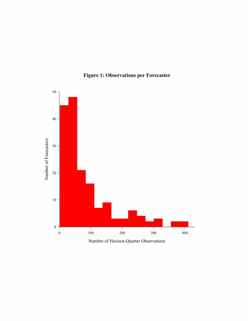
Figure 1: Observations per Forecaster
Number of Horizon-Quarter Observations
0 100 200 300 400
Num
ber o
f For
ecas
ters
0
10
20
30
40
50

Table 1: Linear Forecast Regression
Ejt−hrt = dhj + bπEjt−hπt+1 + bxEjt−hxt+1
Ints. b̂π b̂x R2
(se) (se)
dhj 0.774 -0.026 0.628(0.020) (0.013)
dh, dj 0.742 -0.030 0.618(0.019) (0.012)
dj 0.743 -0.030 0.618(0.019) (0.012)
dh 1.178 -0.002 0.451(0.016) (0.014)
d 1.178 -0.003 0.451(0.016) (0.014)
Notes: {j,t,h} index forecaster, time period,and horizon. Ints. is the set of intercepts.There are 14727 observations for 1981:1-2007:3.
23
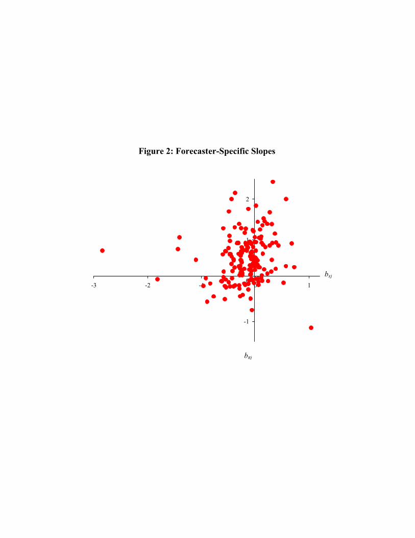
Figure 2: Forecaster-Specific Slopes
-3 -2 -1 0 1
-1
0
1
2
bxj
b j
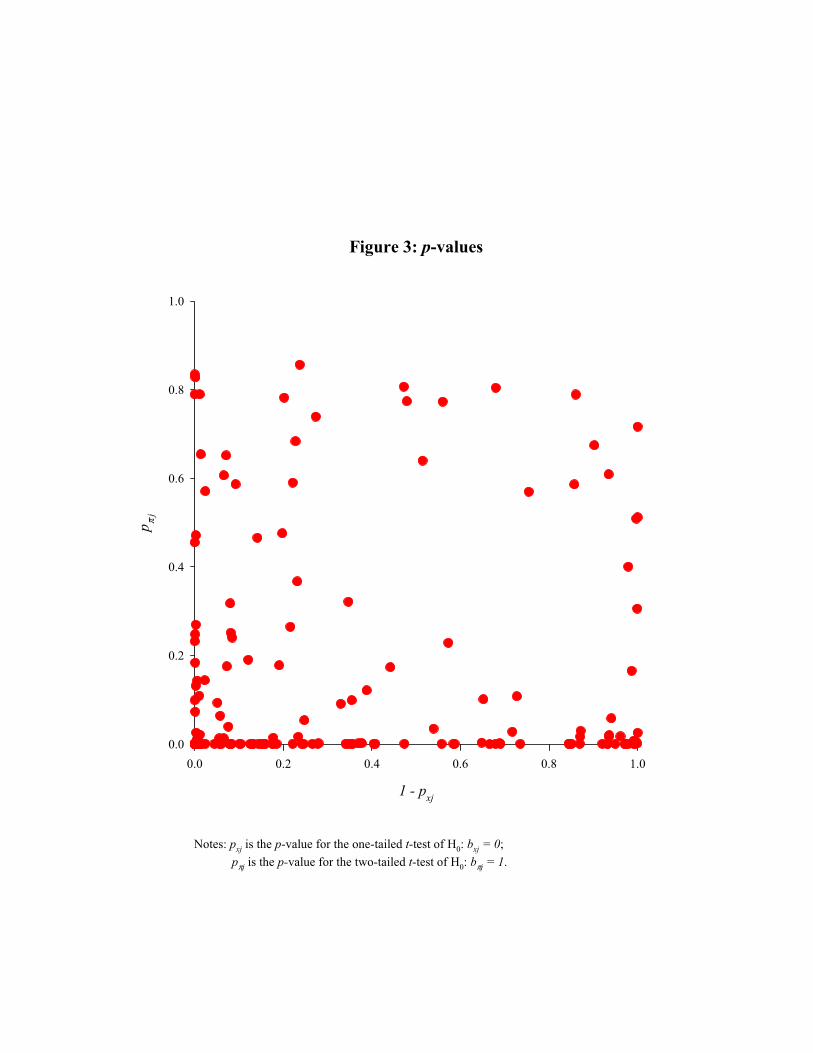
Figure 3: p-values
1 - pxj
0.0 0.2 0.4 0.6 0.8 1.0
p π j
0.0
0.2
0.4
0.6
0.8
1.0
Notes: pxj is the p-value for the one-tailed t-test of H0: bxj = 0;pπj is the p-value for the two-tailed t-test of H0: bπj = 1.
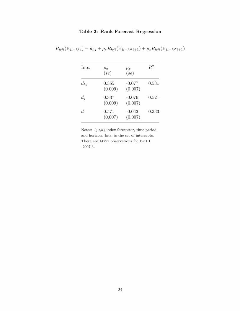
Table 2: Rank Forecast Regression
Rhjt(Ejt−hrt) = dhj + ρπRhjt(Ejt−hπt+1) + ρxRhjt(Ejt−hxt+1)
Ints. ρπ ρx R2
(se) (se)
dhj 0.355 -0.077 0.531(0.009) (0.007)
dj 0.337 -0.076 0.521(0.009) (0.007)
d 0.571 -0.043 0.333(0.007) (0.007)
Notes: {j,t,h} index forecaster, time period,and horizon. Ints. is the set of intercepts.There are 14727 observations for 1981:1-2007:3.
24
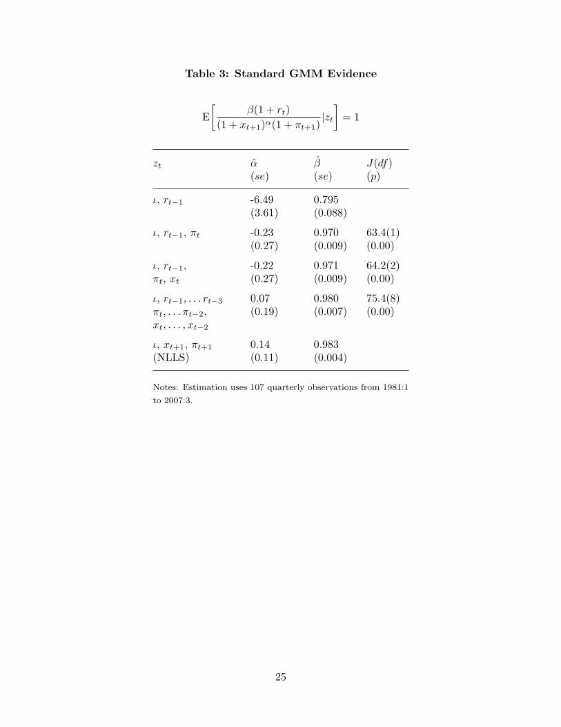
Table 3: Standard GMM Evidence
E[
β(1 + rt)(1 + xt+1)α(1 + πt+1)
|zt
]= 1
zt α̂ β̂ J(df)(se) (se) (p)
ι, rt−1 -6.49 0.795(3.61) (0.088)
ι, rt−1, πt -0.23 0.970 63.4(1)(0.27) (0.009) (0.00)
ι, rt−1, -0.22 0.971 64.2(2)πt, xt (0.27) (0.009) (0.00)
ι, rt−1, . . . rt−3 0.07 0.980 75.4(8)πt, . . . πt−2, (0.19) (0.007) (0.00)xt, . . . , xt−2
ι, xt+1, πt+1 0.14 0.983(NLLS) (0.11) (0.004)
Notes: Estimation uses 107 quarterly observations from 1981:1to 2007:3.
25

Table 4: Linear GMM Evidence
E[ln(1 + rt) − d − ln(1 + πt+1) − bx ln(1 + xt+1)|zt
]= 0
zt b̂x J(df)(se) (p)
ι, ln(1 + rt−1) -10.6(12.2)
ι, ln(1 + rt−1), ln(1 + πt) -0.01 67.9(1)(0.26) (0.00)
ι, ln(1 + rt−1), ln(1 + πt), 0.01 68.4(2)ln(1 + xt) (0.26) (0.00)
ι, ln(1 + rt−1), . . . ln(1 + rt−3) 0.18 75.4(8)ln(1 + πt), . . . ln(1 + πt−2), (0.19) (0.00)ln(1 + xt), . . . , ln(1 + xt−2)
ι, ln(1 + πt+1), ln(1 + xt+1) -0.86(OLS) (0.37)
Notes: Estimation uses 107 quarterly observations from 1981:1to 2007:3.
26
Related Documents