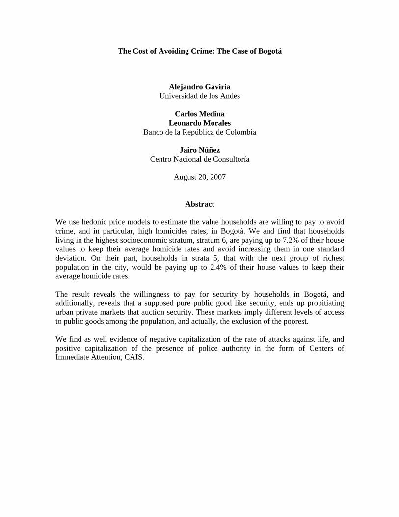
The Cost of Avoiding Crime: The Case of Bogot

The Cost of Avoiding Crime: The Case of Bogotá

Alejandro Gaviria Universidad de los Andes

Carlos Medina

Leonardo Morales Banco de la República de Colombia

Jairo Núñez

Centro Nacional de Consultoría

August 20, 2007

Abstract

We use hedonic price models to estimate the value households are willing to pay to avoid crime, and in particular, high homicides rates, in Bogotá. We and find that households living in the highest socioeconomic stratum, stratum 6, are paying up to 7.2% of their house values to keep their average homicide rates and avoid increasing them in one standard deviation. On their part, households in strata 5, that with the next group of richest population in the city, would be paying up to 2.4% of their house values to keep their average homicide rates. The result reveals the willingness to pay for security by households in Bogotá, and additionally, reveals that a supposed pure public good like security, ends up propitiating urban private markets that auction security. These markets imply different levels of access to public goods among the population, and actually, the exclusion of the poorest. We find as well evidence of negative capitalization of the rate of attacks against life, and positive capitalization of the presence of police authority in the form of Centers of Immediate Attention, CAIS.

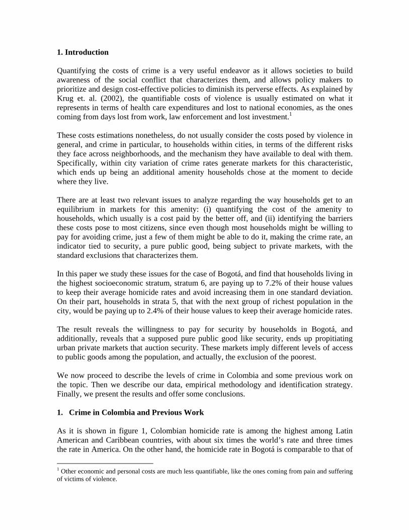
1. Introduction Quantifying the costs of crime is a very useful endeavor as it allows societies to build awareness of the social conflict that characterizes them, and allows policy makers to prioritize and design cost-effective policies to diminish its perverse effects. As explained by Krug et. al. (2002), the quantifiable costs of violence is usually estimated on what it represents in terms of health care expenditures and lost to national economies, as the ones coming from days lost from work, law enforcement and lost investment.1 These costs estimations nonetheless, do not usually consider the costs posed by violence in general, and crime in particular, to households within cities, in terms of the different risks they face across neighborhoods, and the mechanism they have available to deal with them. Specifically, within city variation of crime rates generate markets for this characteristic, which ends up being an additional amenity households chose at the moment to decide where they live. There are at least two relevant issues to analyze regarding the way households get to an equilibrium in markets for this amenity: (i) quantifying the cost of the amenity to households, which usually is a cost paid by the better off, and (ii) identifying the barriers these costs pose to most citizens, since even though most households might be willing to pay for avoiding crime, just a few of them might be able to do it, making the crime rate, an indicator tied to security, a pure public good, being subject to private markets, with the standard exclusions that characterizes them. In this paper we study these issues for the case of Bogotá, and find that households living in the highest socioeconomic stratum, stratum 6, are paying up to 7.2% of their house values to keep their average homicide rates and avoid increasing them in one standard deviation. On their part, households in strata 5, that with the next group of richest population in the city, would be paying up to 2.4% of their house values to keep their average homicide rates. The result reveals the willingness to pay for security by households in Bogotá, and additionally, reveals that a supposed pure public good like security, ends up propitiating urban private markets that auction security. These markets imply different levels of access to public goods among the population, and actually, the exclusion of the poorest. We now proceed to describe the levels of crime in Colombia and some previous work on the topic. Then we describe our data, empirical methodology and identification strategy. Finally, we present the results and offer some conclusions. 1. Crime in Colombia and Previous Work As it is shown in figure 1, Colombian homicide rate is among the highest among Latin American and Caribbean countries, with about six times the world’s rate and three times the rate in America. On the other hand, the homicide rate in Bogotá is comparable to that of

1 Other economic and personal costs are much less quantifiable, like the ones coming from pain and suffering of victims of violence.

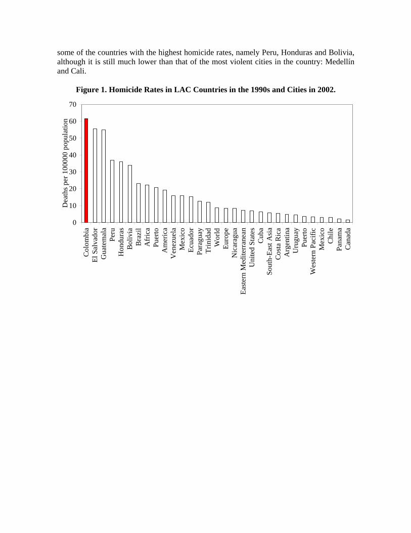
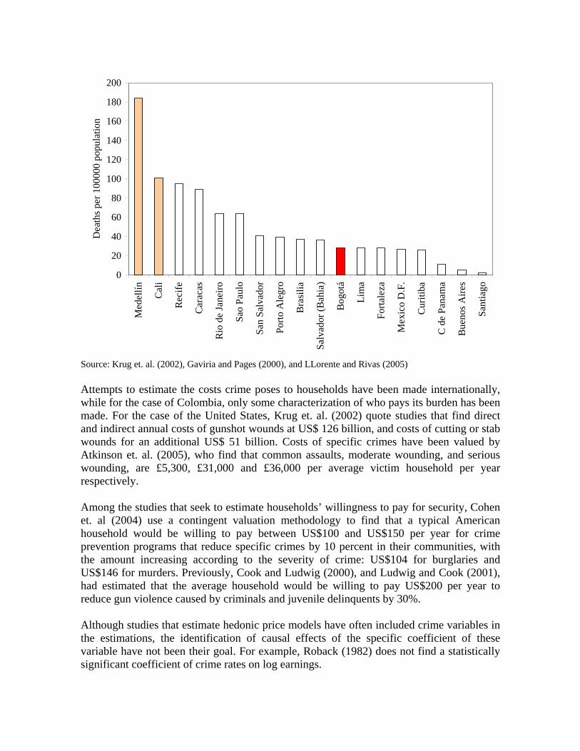
some of the countries with the highest homicide rates, namely Peru, Honduras and Bolivia, although it is still much lower than that of the most violent cities in the country: Medellín and Cali.

Figure 1. Homicide Rates in LAC Countries in the 1990s and Cities in 2002.

0

10

20

30

40

50

60

70

Col

ombi

aEl

Sal

vado

rG

uate

mal

aPe

ruH

ondu

ras

Bol

ivia

Bra

zil

Afr

ica

Puer

toA

mer

ica

Ven

ezue

laM

exic

oEc

uado

rPa

ragu

ayTr

inid

adW

orld

Euro

peN

icar

agua

East

ern

Med

iterr

anea

nU

nite

d St

ates

Cub

aSo

uth-

East

Asi

aC

osta

Ric

aA

rgen

tina

Uru

guay

Puer

toW

este

rn P

acifi

cM

exic

oC

hile

Pana

ma

Can

ada

Dea

ths p

er 1

0000

0 po

pula

tion

0

20

40

60

80

100

120

140

160

180

200

Med

ellín Cal

i

Rec

ife

Car

acas

Rio

de

Jane

iro

Sao

Paul

o

San

Salv

ador

Porto

Ale

gro

Bra

silia

Salv

ador

(Bah

ia)

Bog

otá

Lim

a

Forta

leza

Mex

ico

D.F

.

Cur

itiba

C d

e Pa

nam

a

Bue

nos A

ires

Sant

iago

Dea

ths p

er 1

0000

0 po

pula

tion

Source: Krug et. al. (2002), Gaviria and Pages (2000), and LLorente and Rivas (2005) Attempts to estimate the costs crime poses to households have been made internationally, while for the case of Colombia, only some characterization of who pays its burden has been made. For the case of the United States, Krug et. al. (2002) quote studies that find direct and indirect annual costs of gunshot wounds at US$ 126 billion, and costs of cutting or stab wounds for an additional US$ 51 billion. Costs of specific crimes have been valued by Atkinson et. al. (2005), who find that common assaults, moderate wounding, and serious wounding, are £5,300, £31,000 and £36,000 per average victim household per year respectively. Among the studies that seek to estimate households’ willingness to pay for security, Cohen et. al (2004) use a contingent valuation methodology to find that a typical American household would be willing to pay between US$100 and US$150 per year for crime prevention programs that reduce specific crimes by 10 percent in their communities, with the amount increasing according to the severity of crime: US$104 for burglaries and US$146 for murders. Previously, Cook and Ludwig (2000), and Ludwig and Cook (2001), had estimated that the average household would be willing to pay US$200 per year to reduce gun violence caused by criminals and juvenile delinquents by 30%. Although studies that estimate hedonic price models have often included crime variables in the estimations, the identification of causal effects of the specific coefficient of these variable have not been their goal. For example, Roback (1982) does not find a statistically significant coefficient of crime rates on log earnings.

For Colombia, the closest attempt to quantify distributional effects of crime variables is that of Gaviria and Velez (2001), who find that rich households are more likely to be victims of property crime, to modify their behavior for fear of crime, to feel unsafe in the cities, and to invest more in crime avoidance, while the poorest are more likely to be victims of homicides and domestic violence, and the richest of kidnapping. Other studies have focused in estimating the economic costs of violence in Colombia. Trujillo and Badel (1998) estimated the gross costs of urban criminality and armed conflict in Colombia between 1991 and 1996 in 4.25% of GDP. Badel (1999) estimated the gross direct costs of violence and armed conflict between 1990 and 1998 in 4.5% of GDP. Londoño and Guerrero (2000) estimate the direct costs of violence on health (medical attention and lost years of life) and material lost (public and private security, and justice) in 4.9% of GDP for a subset of Latin American and Caribbean countries, and 11.4% of GDP for Colombia (5.0% in health, and 6.4% in material loses). Furthermore, their estimate of indirect costs of violence (productivity, investment, work and consumption) and transfers, amount to 9.2% of GDP for the same countries, and 13.3% of GDP for Colombia. These studies nonetheless, did not quantify the willingness to pay of household to avoid urban violence the way we do. An area in which more evidence has been collected for violence in Colombia, and in particular, in Bogotá, is the related to spatial patterns of crime. Núñez and Sánchez (2001) find statistically significant spatial correlation for objects theft, assaults, cars theft, residential and commercial theft rates. Similarly, Llorente et. al. (2001) illustrate graphically the spatial segregation of homicides in Bogotá, and additionally, study its dynamics, finding that homicides are spatially very persistent, they take place mostly around the same places of the city with different degrees of intensity. In what follows, we use several of this literature and provide additional elements that support our assumptions in the estimations of the costs homicide rates pose on house values and rents. We continue describing the data used for our exercise, before proceeding to present the methodology and results of the empirical model. 3. Data2

Map 1. Localidades of Bogotá.3We use data at the household level from the Encuesta de Calidad de Vida, collected by the Administrative Department of National Statistics of Colombia, DANE, in 2003.4 That LSMS survey, has detailed information about living conditions of household in Bogotá,

2 This section builds heavily on Medina et. al. (2007) 3 Source: Medina et. al. (2007) 4 The survey was collected between June 6 and July 23. Household members 18 and older were directly interviewed.

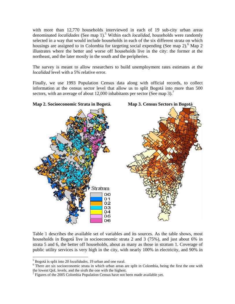
with more than 12,770 households interviewed in each of 19 sub-city urban areas denominated localidades (See map 1).5 Within each localidad, households were randomly selected in a way that would include households in each of the six different strata on which housings are assigned to in Colombia for targeting social expending (See map 2).6 Map 2 illustrates where the better and worse off households live in the city: the former at the northeast, and the later mostly in the south and the peripheries. The survey is meant to allow researchers to build unemployment rates estimates at the localidad level with a 5% relative error. Finally, we use 1993 Population Census data along with official records, to collect information at the census sector level that allow us to split Bogotá into more than 500 sectors, with an average of about 12,000 inhabitants per sector (See map 3).7 Map 2. Socioeconomic Strata in Bogotá. Map 3. Census Sectors in Bogotá

Table 1 describes the available set of variables and its sources. As the table shows, most households in Bogotá live in socioeconomic strata 2 and 3 (75%), and just about 6% in strata 5 and 6, the better off households, about as many as those in stratum 1. Coverage of public utility services is very high in the city, with nearly 100% in electricity, and 90% in 5 Bogotá is split into 20 localidades, 19 urban and one rural. 6 There are six socioeconomic strata in which urban areas are split in Colombia, being the first the one with the lowest QoL levels, and the sixth the one with the highest. 7 Figures of the 2005 Colombia Population Census have not been made available yet.

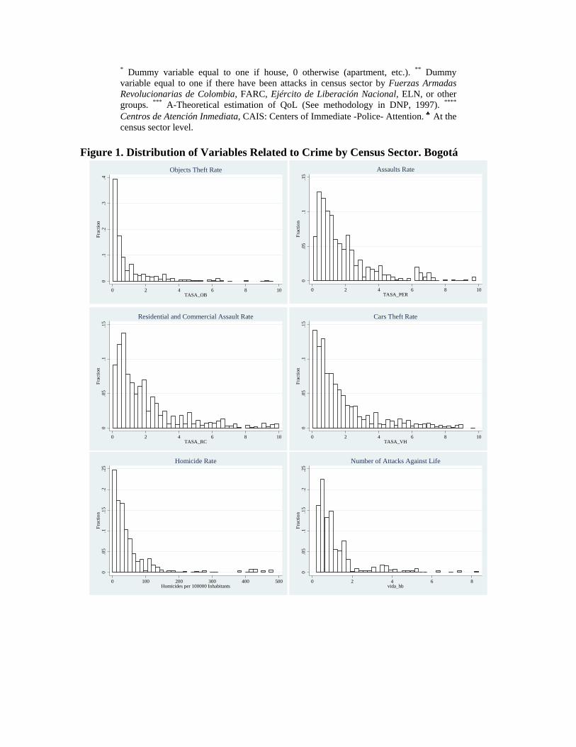
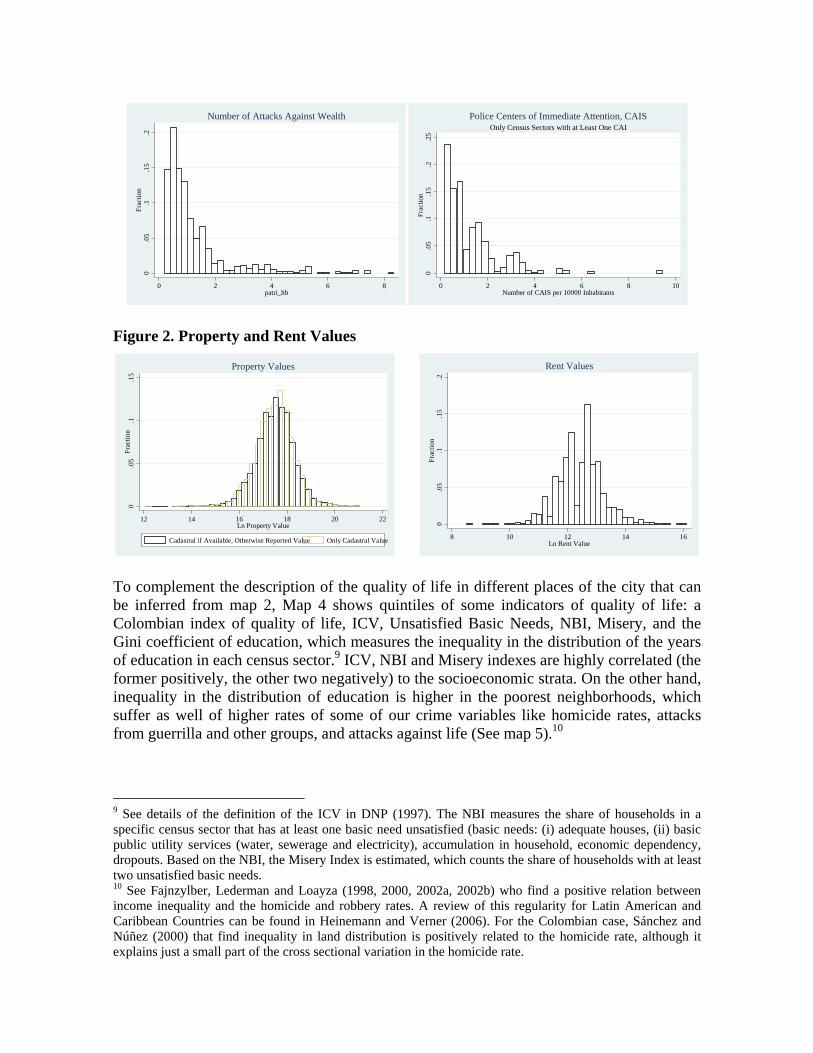
fixed phone lines. It will become important, at the moment of interpreting our results, to bear in mind that the higher socioeconomic strata have nearly 100% coverage in fixed phone lines, thus, remaining variation of that variable will be privative of the poorest strata, which implies that such variable might partially work as a proxy for poverty. As shown in the table, we have cadastral data for nearly 70% of the households. Our variables related to crime, include objects theft rate, assaults rate, residential and commercial assaults rate, cars theft rate, homicide rate, attacks of terrorists groups, attacks against life, and attacks against wealth.8 The distribution of these variables is illustrated in figure 1, where it becomes clear how skewed they are, in particular, the objects theft and homicide rates. The police Center of Immediate Attention, CAIS, have a similar shape. We have cadastral data on property values for close to 8900 houses in Bogotá. In addition, we have household’s reported property values for households owning houses where they live. Reported rent prices are available for houses living as tenants (how much do you pay?) and for those living in their own house (how much would you pay if it was rented?). As it can be seen in figure 2, the distribution of property values obtained of using exclusively cadastral data is very similar to the one obtained when it is complemented with household reported data from the ECV survey.

8 For the purposes of this study, we understand homicides as the activity by jeans of which un person kills another. (Art. 323 penal Code), attacks against life, as hurting someone’s body or health (Art. 332 Código Penal), and objects theft as the act of substracting someone else’s goods for own benefit. (Art. 349 Penal Code).

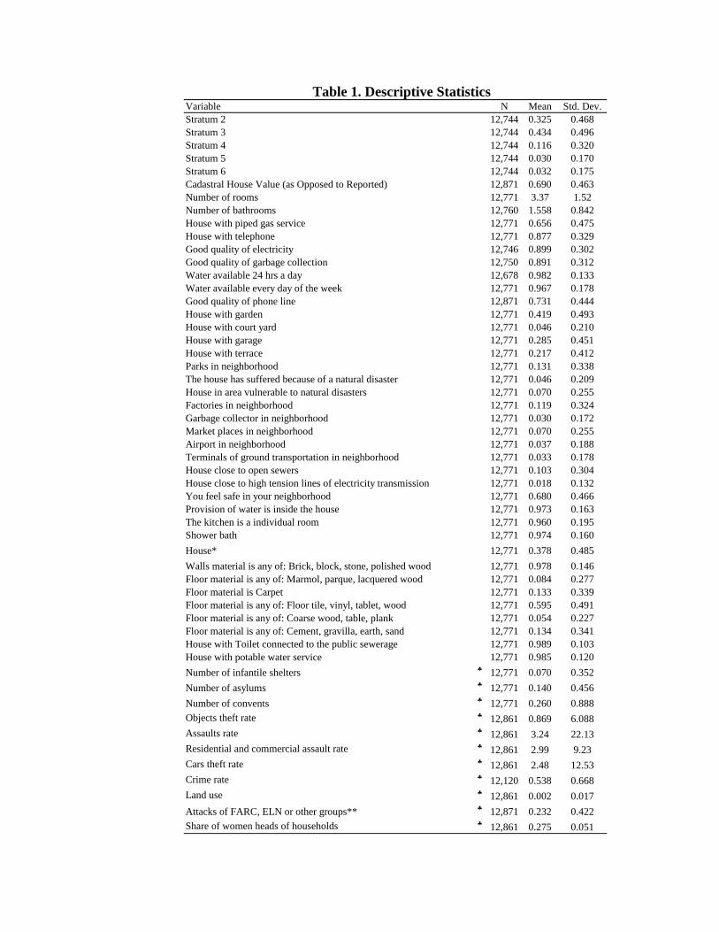
Table 1. Descriptive Statistics Variable N Mean Std. Dev.Stratum 2 12,744 0.325 0.468Stratum 3 12,744 0.434 0.496Stratum 4 12,744 0.116 0.320Stratum 5 12,744 0.030 0.170Stratum 6 12,744 0.032 0.175Cadastral House Value (as Opposed to Reported) 12,871 0.690 0.463Number of rooms 12,771 3.37 1.52Number of bathrooms 12,760 1.558 0.842House with piped gas service 12,771 0.656 0.475House with telephone 12,771 0.877 0.329Good quality of electricity 12,746 0.899 0.302Good quality of garbage collection 12,750 0.891 0.312Water available 24 hrs a day 12,678 0.982 0.133Water available every day of the week 12,771 0.967 0.178Good quality of phone line 12,871 0.731 0.444House with garden 12,771 0.419 0.493House with court yard 12,771 0.046 0.210House with garage 12,771 0.285 0.451House with terrace 12,771 0.217 0.412Parks in neighborhood 12,771 0.131 0.338The house has suffered because of a natural disaster 12,771 0.046 0.209House in area vulnerable to natural disasters 12,771 0.070 0.255Factories in neighborhood 12,771 0.119 0.324Garbage collector in neighborhood 12,771 0.030 0.172Market places in neighborhood 12,771 0.070 0.255Airport in neighborhood 12,771 0.037 0.188Terminals of ground transportation in neighborhood 12,771 0.033 0.178House close to open sewers 12,771 0.103 0.304House close to high tension lines of electricity transmission 12,771 0.018 0.132You feel safe in your neighborhood 12,771 0.680 0.466Provision of water is inside the house 12,771 0.973 0.163The kitchen is a individual room 12,771 0.960 0.195Shower bath 12,771 0.974 0.160House* 12,771 0.378 0.485Walls material is any of: Brick, block, stone, polished wood 12,771 0.978 0.146Floor material is any of: Marmol, parque, lacquered wood 12,771 0.084 0.277Floor material is Carpet 12,771 0.133 0.339Floor material is any of: Floor tile, vinyl, tablet, wood 12,771 0.595 0.491Floor material is any of: Coarse wood, table, plank 12,771 0.054 0.227Floor material is any of: Cement, gravilla, earth, sand 12,771 0.134 0.341House with Toilet connected to the public sewerage 12,771 0.989 0.103House with potable water service 12,771 0.985 0.120Number of infantile shelters ♣ 12,771 0.070 0.352Number of asylums ♣ 12,771 0.140 0.456Number of convents ♣ 12,771 0.260 0.888Objects theft rate ♣ 12,861 0.869 6.088Assaults rate ♣ 12,861 3.24 22.13Residential and commercial assault rate ♣ 12,861 2.99 9.23Cars theft rate ♣ 12,861 2.48 12.53Crime rate ♣ 12,120 0.538 0.668Land use ♣ 12,861 0.002 0.017Attacks of FARC, ELN or other groups** ♣ 12,871 0.232 0.422Share of women heads of households ♣ 12,861 0.275 0.051

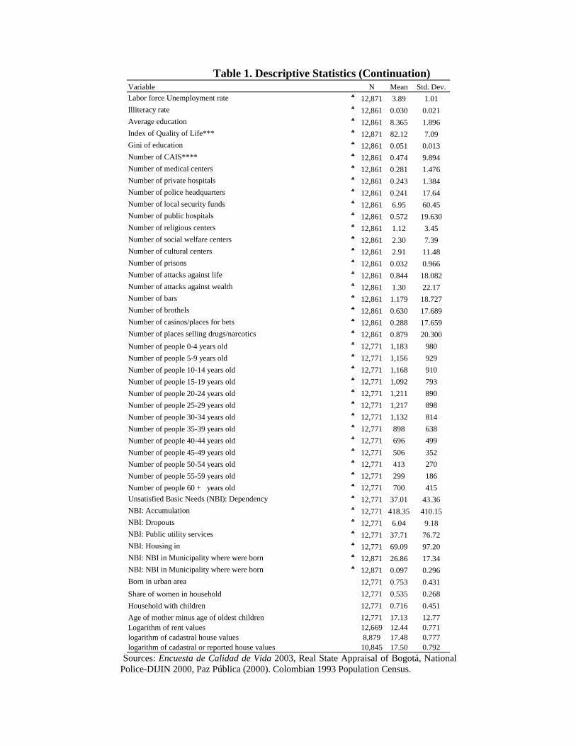
Table 1. Descriptive Statistics (Continuation)

Sources: Encuesta de Calidad de Vida 2003, Real State Appraisal of Bogotá, National Police-DIJIN 2000, Paz Pública (2000). Colombian 1993 Population Census.

Variable N Mean Std. Dev.Labor force Unemployment rate ♣ 12,871 3.89 1.01Illiteracy rate ♣ 12,861 0.030 0.021Average education ♣ 12,861 8.365 1.896Index of Quality of Life*** ♣ 12,871 82.12 7.09Gini of education ♣ 12,861 0.051 0.013Number of CAIS**** ♣ 12,861 0.474 9.894Number of medical centers ♣ 12,861 0.281 1.476Number of private hospitals ♣ 12,861 0.243 1.384Number of police headquarters ♣ 12,861 0.241 17.64Number of local security funds ♣ 12,861 6.95 60.45Number of public hospitals ♣ 12,861 0.572 19.630Number of religious centers ♣ 12,861 1.12 3.45Number of social welfare centers ♣ 12,861 2.30 7.39Number of cultural centers ♣ 12,861 2.91 11.48Number of prisons ♣ 12,861 0.032 0.966Number of attacks against life ♣ 12,861 0.844 18.082Number of attacks against wealth ♣ 12,861 1.30 22.17Number of bars ♣ 12,861 1.179 18.727Number of brothels ♣ 12,861 0.630 17.689Number of casinos/places for bets ♣ 12,861 0.288 17.659Number of places selling drugs/narcotics ♣ 12,861 0.879 20.300Number of people 0-4 years old ♣ 12,771 1,183 980Number of people 5-9 years old ♣ 12,771 1,156 929Number of people 10-14 years old ♣ 12,771 1,168 910Number of people 15-19 years old ♣ 12,771 1,092 793Number of people 20-24 years old ♣ 12,771 1,211 890Number of people 25-29 years old ♣ 12,771 1,217 898Number of people 30-34 years old ♣ 12,771 1,132 814Number of people 35-39 years old ♣ 12,771 898 638Number of people 40-44 years old ♣ 12,771 696 499Number of people 45-49 years old ♣ 12,771 506 352Number of people 50-54 years old ♣ 12,771 413 270Number of people 55-59 years old ♣ 12,771 299 186Number of people 60 + years old ♣ 12,771 700 415Unsatisfied Basic Needs (NBI): Dependency ♣ 12,771 37.01 43.36NBI: Accumulation ♣ 12,771 418.35 410.15NBI: Dropouts ♣ 12,771 6.04 9.18NBI: Public utility services ♣ 12,771 37.71 76.72NBI: Housing in ♣ 12,771 69.09 97.20NBI: NBI in Municipality where were born ♣ 12,871 26.86 17.34NBI: NBI in Municipality where were born ♣ 12,871 0.097 0.296Born in urban area 12,771 0.753 0.431Share of women in household 12,771 0.535 0.268Household with children 12,771 0.716 0.451Age of mother minus age of oldest children 12,771 17.13 12.77Logarithm of rent values 12,669 12.44 0.771logarithm of cadastral house values 8,879 17.48 0.777logarithm of cadastral or reported house values 10,845 17.50 0.792

* Dummy variable equal to one if house, 0 otherwise (apartment, etc.). ** Dummy variable equal to one if there have been attacks in census sector by Fuerzas Armadas Revolucionarias de Colombia, FARC, Ejército de Liberación Nacional, ELN, or other groups. *** A-Theoretical estimation of QoL (See methodology in DNP, 1997). **** Centros de Atención Inmediata, CAIS: Centers of Immediate -Police- Attention. ♣ At the census sector level.

Figure 1. Distribution of Variables Related to Crime by Census Sector. Bogotá

0.1

.2.3

.4Fr

actio

n

0 2 4 6 8 10TASA_OB

Objects Theft Rate

0.0

5.1

.15

Frac

tion

0 2 4 6 8 10TASA_PER

Assaults Rate

0.0

5.1

.15

Frac

tion

0 2 4 6 8 10TASA_RC

Residential and Commercial Assault Rate

0.0

5.1

.15

Frac

tion

0 2 4 6 8 10TASA_VH

Cars Theft Rate

0.0

5.1

.15

.2.2

5Fr

actio

n

0 100 200 300 400 500Homicides per 100000 Inhabitants

Homicide Rate

0.0

5.1

.15

.2.2

5Fr

actio

n

0 2 4 6 8vida_hb

Number of Attacks Against Life

0.0

5.1

.15

.2Fr

actio

n

0 2 4 6 8patri_hb

Number of Attacks Against Wealth

0.0

5.1

.15

.2.2

5Fr

actio

n

0 2 4 6 8 10Number of CAIS per 10000 Inhabitants

Only Census Sectors with at Least One CAIPolice Centers of Immediate Attention, CAIS

Figure 2. Property and Rent Values

0.0

5.1

.15

.2Fr

actio

n

8 10 12 14 16Ln Rent Value

Rent Values

0.0

5.1

.15

Frac

tion

12 14 16 18 20 22Ln Property Value

Cadastral if Available, Otherwise Reported Value Only Cadastral Value

Property Values

To complement the description of the quality of life in different places of the city that can be inferred from map 2, Map 4 shows quintiles of some indicators of quality of life: a Colombian index of quality of life, ICV, Unsatisfied Basic Needs, NBI, Misery, and the Gini coefficient of education, which measures the inequality in the distribution of the years of education in each census sector.9 ICV, NBI and Misery indexes are highly correlated (the former positively, the other two negatively) to the socioeconomic strata. On the other hand, inequality in the distribution of education is higher in the poorest neighborhoods, which suffer as well of higher rates of some of our crime variables like homicide rates, attacks from guerrilla and other groups, and attacks against life (See map 5).10

9 See details of the definition of the ICV in DNP (1997). The NBI measures the share of households in a specific census sector that has at least one basic need unsatisfied (basic needs: (i) adequate houses, (ii) basic public utility services (water, sewerage and electricity), accumulation in household, economic dependency, dropouts. Based on the NBI, the Misery Index is estimated, which counts the share of households with at least two unsatisfied basic needs. 10 See Fajnzylber, Lederman and Loayza (1998, 2000, 2002a, 2002b) who find a positive relation between income inequality and the homicide and robbery rates. A review of this regularity for Latin American and Caribbean Countries can be found in Heinemann and Verner (2006). For the Colombian case, Sánchez and Núñez (2000) that find inequality in land distribution is positively related to the homicide rate, although it explains just a small part of the cross sectional variation in the homicide rate.

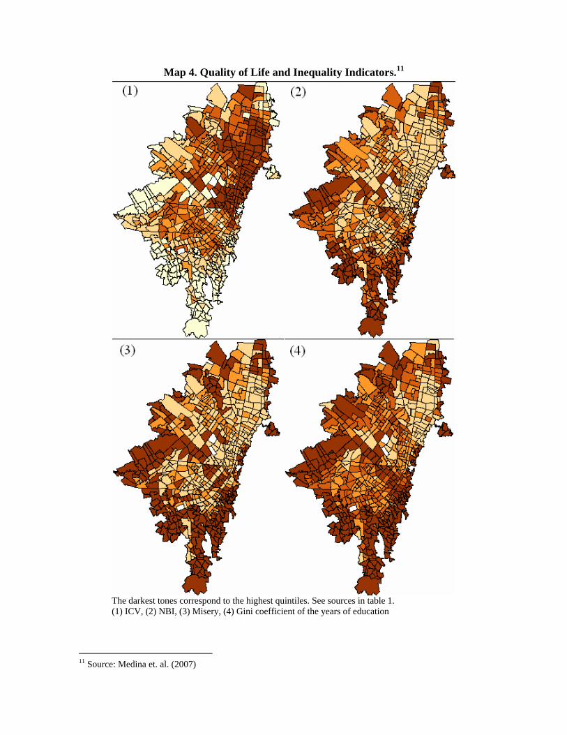
Map 4. Quality of Life and Inequality Indicators.11

The darkest tones correspond to the highest quintiles. See sources in table 1. (1) ICV, (2) NBI, (3) Misery, (4) Gini coefficient of the years of education

11 Source: Medina et. al. (2007)

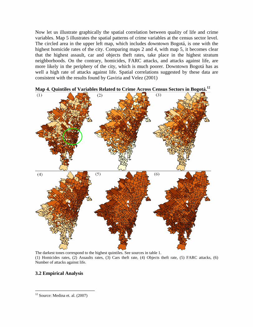
Now let us illustrate graphically the spatial correlation between quality of life and crime variables. Map 5 illustrates the spatial patterns of crime variables at the census sector level. The circled area in the upper left map, which includes downtown Bogotá, is one with the highest homicide rates of the city. Comparing maps 2 and 4, with map 5, it becomes clear that the highest assault, car and objects theft rates, take place in the highest stratum neighborhoods. On the contrary, homicides, FARC attacks, and attacks against life, are more likely in the periphery of the city, which is much poorer. Downtown Bogotá has as well a high rate of attacks against life. Spatial correlations suggested by these data are consistent with the results found by Gaviria and Velez (2001) Map 4. Quintiles of Variables Related to Crime Across Census Sectors in Bogotá.12

The darkest tones correspond to the highest quintiles. See sources in table 1. (1) Homicides rates, (2) Assaults rates, (3) Cars theft rate, (4) Objects theft rate, (5) FARC attacks, (6) Number of attacks against life. 3.2 Empirical Analysis

12 Source: Medina et. al. (2007)

( ) ijjiij uAHP +++= 210ln ααα

In this section we estimate the amount household would be willing to pay to avoid crime. We estimate a hedonic regression model of the logarithm of house valuation, and rental prices, on a battery of household and amenities variables, of the form

( ) ijjiij uAHP +++= 210ln ααα ( )1Where Pij is either the value of the house (cadastral or reported by household) or rent (reported by household), Hi is a vector of household i variables, and Aj is a vector of amenities in census sector j. The idea is that the price households pay for their houses is compensated for what they get in house characteristics and amenities, amenities including access and quality of public goods and services (roads, parks and other green space, good weather, transport, security, etc.). In equilibrium, amenities would be capitalized into house values and rents.13

Table 2 presents the results of estimating this equation using different sources for the dependent variable. First, we present the results of using as our dependent variable the cadastral value of houses for those houses we have it available, and the amount reported by the household for those we do not have cadastral values, adding up to 10,290 households. The following panel presents the results of estimating the hedonic regression with only those households for which we have the cadastral values, namely 8,435 households. Finally, the last panel reports the results obtained from estimating the model with the rental values, available for 12,024 households. Each panel contains both OLS and 2SLS results. For all regressions we estimate robust standard errors correcting for clustering at the census sector level. We focus first on the OLS estimates. Overall, the estimates found present intuitive signs. As it is shown, the value/rent of houses increases for houses located in better socioeconomic strata, for houses with better characteristics, such as their number of rooms, of bathrooms, if the house has piped gas, garden, garage, kitchen in an individual room, better floor materials, if there are parks in their neighborhood, and there are no open sewers, no garbage collectors, and house with potable water. Note that in the first panel, where we use cadastral values for those houses we have it available, and reported values for those we do not have the cadastral ones, we include a dummy variable equal to one if the house value is the cadastral and zero otherwise. The coefficient of this variable implies that cadastral values are on average 10.6% lower than the commercial values reported by households in the survey. Regarding the variables related to crime, the objects theft rate is negatively related to house value, but its sign is only statistically significant for rent values. Attacks against life are as well negatively related to house values, although in that case, the sign is significant only for house values. The variable attacks by FARC, ELN, and other groups, is weakly negatively related to house rent. On the other hand, the assaults, residential and commercial assaults, cars thefts and crime rates, are unrelated to house values. Finally, the attacks against wealth are positively related to house values.

13 See Rosen (1971, 1974, 2002), Blomquist et. al. (1982), Roback (1982, 1988), and Gyourko et. al. (1999) among others.

Although we would expect all crime related variables to be negatively related to house values and rents, there are several sources of endogeneity that would be preventing us from getting the expected results. On the one hand, if places where crimes are more likely to happen are the better neighborhoods, omitted characteristics of the neighborhoods might be positively correlated to these crimes, for example, cars theft, which would overestimate the coefficients of interest. On the other hand, some crimes like homicides, might take place more often in poor neighborhoods because the richest are more like to count with much better security, which should be already capitalized in house values and rents. To minimize the omitted variable bias problem, we estimate again equation (1) interacting variables included in table 2 with the socioeconomic strata.14 Results for the crime related variables are presented in table 3. According to the previous results, households who report feeling safe in their neighborhoods pay less rent for their houses, a result that weakly follows for house values in strata 5, once we include interactions. Nonetheless, this result might be driven by differences in perceptions between the richest and the poorest: if the richest live in safer neighborhoods and yet they do not feel as safe as the poorest, the coefficient would be capturing more these differences in perceptions than the capitalization of security. Once we include the interactions with socioeconomic strata, the objects theft rate reveal a pattern of negative capitalization as we move towards the higher strata. Other variables like assaults, residential and commercial assaults, crime rates, attacks by FARC, ELN, and other groups, and attacks against wealth, show no relation to house or rent values. Actually, cars theft and crime rates become positive and significant when interacted with stratum 6. The variable attacks against life keep registering a negative relation to house values and rents. The variable number of Centers of Immediate Attention, CAIS, which appeared only positively related to house rents, become positively and significantly related to house values when interacted with the highest socioeconomic strata, and only weakly positively related to house rents. Instrumenting the Crime Rate In this section we try to identify the capitalization effect of the crime rate on house values and rents, by using an instrumental variable approach. The goal is to use a variable related to the decision the households make of living in a neighborhood of a determined crime rate, while at the same time not affecting the value or rent of the house.

14 The variables “Cadastral”, “You feel safe in Neighborhood”, “Land use”, “Attacks of FARC, ELN, or other groups”, “Number of medical centers”, “Number of medical centers”, “Number of private hospitals”, “Number of police headquarters”, “Number of local security funds”, “Number of public hospitals”, “Number of religious centers”, “Number of social welfare centers”, “Number of cultural centers”, “Number of prisons”, “Number of attacks against life”, “Number of attacks against wealth”, “Number of bars”, “Number of brothels”, “Number of casinos/places for bets”, “Number of places selling drugs/narcotics”, “Number of people by age range”, and the dummy variables of father’s and mother’s education levels and their interactions, are not interacted with the socioeconomic strata.

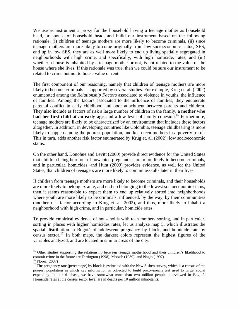
We use as instrument a proxy for the household having a teenage mother as household head, or spouse of household head, and build our instrument based on the following rationale: (i) children of teenage mothers are more likely to become criminals, (ii) since teenage mothers are more likely to come originally from low socioeconomic status, SES, end up in low SES, they are as well more likely to end up living spatially segregated in neighborhoods with high crime, and specifically, with high homicide, rates, and (iii) whether a house is inhabited by a teenage mother or not, is not related to the value of the house where she lives. If this rationale was true, then we could be sure our instrument to be related to crime but not to house value or rent. The first component of our reasoning, namely that children of teenage mothers are more likely to become criminals is supported by several studies. For example, Krug et. al. (2002) enumerated among the Relationship Factors associated to violence in youths, the influence of families. Among the factors associated to the influence of families, they enumerate parental conflict in early childhood and poor attachment between parents and children. They also include as factors of risk a large number of children in the family, a mother who had her first child at an early age, and a low level of family cohesion.15 Furthermore, teenage mothers are likely to be characterized by an environment that includes these factors altogether. In addition, in developing countries like Colombia, teenage childbearing is more likely to happen among the poorest population, and keep teen mothers in a poverty trap.16 This in turn, adds another risk factor enumerated by Krug et. al. (2002): low socioeconomic status. On the other hand, Donohue and Levitt (2000) provide direct evidence for the United States that children being born out of unwanted pregnancies are more likely to become criminals, and in particular, homicides, and Hunt (2003) provides evidence, as well for the United States, that children of teenagers are more likely to commit assaults later in their lives. If children from teenage mothers are more likely to become criminals, and their households are more likely to belong ex ante, and end up belonging to the lowest socioeconomic status, then it seems reasonable to expect them to end up relatively sorted into neighborhoods where youth are more likely to be criminals, influenced, by the way, by their communities (another risk factor according to Krug et. al. 2002), and thus, more likely to inhabit a neighborhood with high crime, and in particular, homicide rates. To provide empirical evidence of households with teen mothers sorting, and in particular, sorting in places with higher homicides rates, let us analyze map 5, which illustrates the spatial distribution in Bogotá of adolescent pregnancy by block, and homicide rate by census sector.17 In both maps, the darkest colors represent the highest figures of the variables analyzed, and are located in similar areas of the city. 15 Other studies supporting the relationship between teenage motherhood and their children’s likelihood to commit crime in the future are Farrington (1998), Morash (1989), and Nagin (1997). 16 Flórez (2007) 17 The pregnancy rate (percentage) by block is estimated with the New Sisben survey, which is a census of the poorest population in which key information is collected to build proxy-means test used to target social expending. In our database, we have somewhat more than two million people interviewed in Bogotá. Homicide rates at the census sector level are in deaths per 10 million inhabitants.

As our proxy variable for teenage mothers in household, we estimate de difference between the age of the spouse of the household (or head of household if woman) and her oldest children living in her household.

Map 5. Adolescent pregnancy rate by block (left), and homicide rate by census sector.18

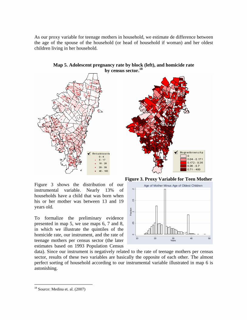
Figure 3. Proxy Variable for Teen Mother Figure 3 shows the distribution of our instrumental variable. Nearly 13% of households have a child that was born when his or her mother was between 13 and 19 years old. To formalize the preliminary evidence presented in map 5, we use maps 6, 7 and 8, in which we illustrate the quintiles of the homicide rate, our instrument, and the rate of teenage mothers per census sector (the later estimates based on 1993 Population Census data). Since our instrument is negatively related to the rate of teenage mothers per census sector, results of these two variables are basically the opposite of each other. The almost perfect sorting of household according to our instrumental variable illustrated in map 6 is astonishing.

0.0

5.1

.15

.2Fr

actio

n

10 20 30 40 50Years

Age of Mother Minus Age of Oldest Children

18 Source: Medina et. al. (2007)

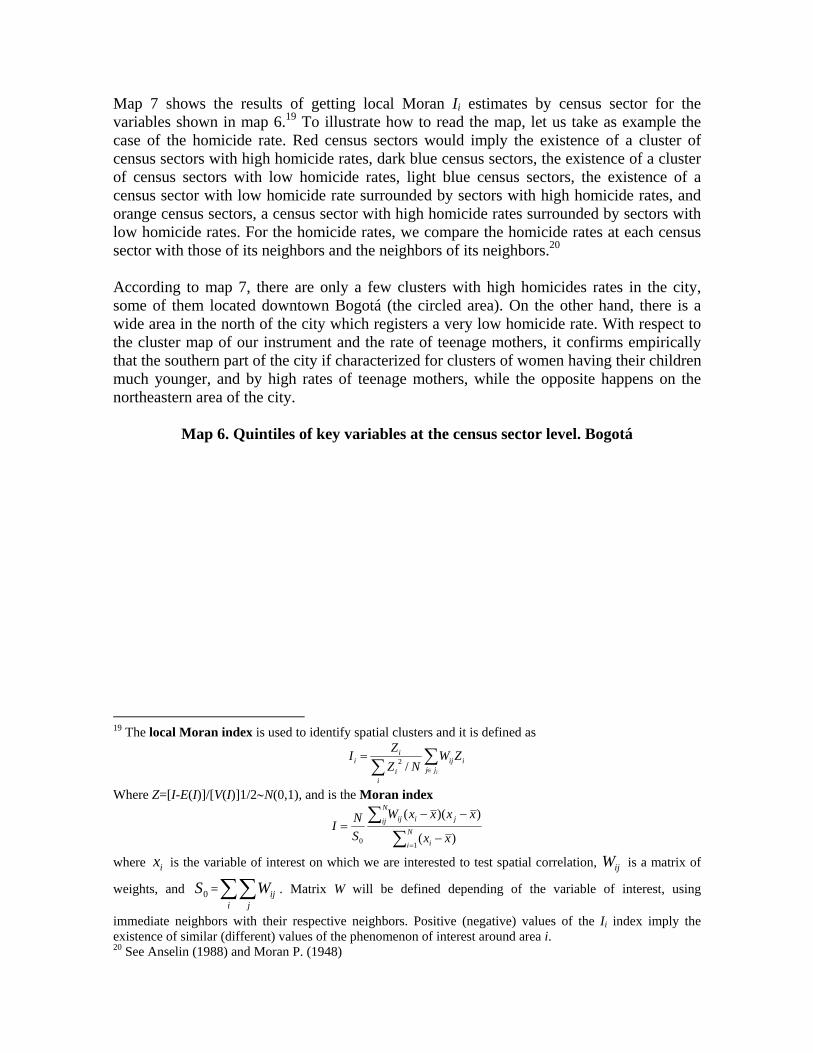
Map 7 shows the results of getting local Moran Ii estimates by census sector for the variables shown in map 6.19 To illustrate how to read the map, let us take as example the case of the homicide rate. Red census sectors would imply the existence of a cluster of census sectors with high homicide rates, dark blue census sectors, the existence of a cluster of census sectors with low homicide rates, light blue census sectors, the existence of a census sector with low homicide rate surrounded by sectors with high homicide rates, and orange census sectors, a census sector with high homicide rates surrounded by sectors with low homicide rates. For the homicide rates, we compare the homicide rates at each census sector with those of its neighbors and the neighbors of its neighbors.20

According to map 7, there are only a few clusters with high homicides rates in the city, some of them located downtown Bogotá (the circled area). On the other hand, there is a wide area in the north of the city which registers a very low homicide rate. With respect to the cluster map of our instrument and the rate of teenage mothers, it confirms empirically that the southern part of the city if characterized for clusters of women having their children much younger, and by high rates of teenage mothers, while the opposite happens on the northeastern area of the city.

Map 6. Quintiles of key variables at the census sector level. Bogotá

19 The local Moran index is used to identify spatial clusters and it is defined as

∑∑ ∈

=ijj

iij

ii

ii ZW

NZZI

/2

Where Z=[I-E(I)]/[V(I)]1/2∼N(0,1), and is the Moran index

∑∑

=−

−−= N

i i

N

ij jiij

xx

xxxxW

SNI

10 )(

))((

where is the variable of interest on which we are interested to test spatial correlation, is a matrix of

weights, and =∑∑ . Matrix W will be defined depending of the variable of interest, using

immediate neighbors with their respective neighbors. Positive (negative) values of the I

ix ijW

0Si j

ijW

i index imply the existence of similar (different) values of the phenomenon of interest around area i. 20 See Anselin (1988) and Moran P. (1948)

Quintiles: (1) homicide rate, (2) age difference: oldest children and mother, (3) rate of teenage mothers

Map 7. Clusters of key variables at the census sector level. Bogotá

Cluster: (1) homicide rate, (2) age difference: oldest children and mother, (3) rate of teenage mothers Finally, map 8 shows that our instrument is negatively correlated to the homicide rate, in a statistically significant magnitude in the south and northeast of the city.21 The same follows for the rate of teenage mothers. The last figure in map 8 illustrates the local spatial covariance between the homicide rates and the share of households with children in the

21 The spatial autocovariance between variables xci and xcj, is estimated with a formula of the form

( ) ( ) ( )( )∑∑= =

−−⎥⎦

⎤⎢⎣

⎡==

N

i

N

jcc

ijcc xxxx

hD

Whfxxjiji

1 1

ˆ,cov

Where x is the sample mean of x, and W(·) is a kernel function normalized to sum one.

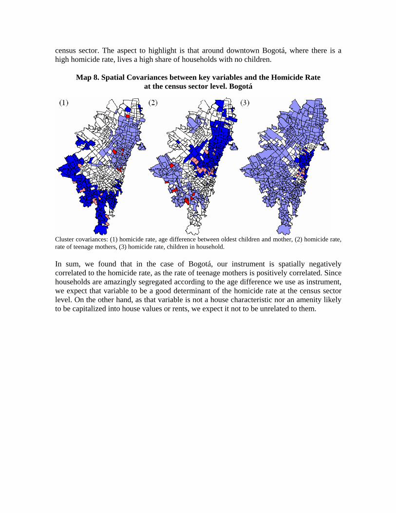
census sector. The aspect to highlight is that around downtown Bogotá, where there is a high homicide rate, lives a high share of households with no children.

Map 8. Spatial Covariances between key variables and the Homicide Rate at the census sector level. Bogotá

Cluster covariances: (1) homicide rate, age difference between oldest children and mother, (2) homicide rate, rate of teenage mothers, (3) homicide rate, children in household. In sum, we found that in the case of Bogotá, our instrument is spatially negatively correlated to the homicide rate, as the rate of teenage mothers is positively correlated. Since households are amazingly segregated according to the age difference we use as instrument, we expect that variable to be a good determinant of the homicide rate at the census sector level. On the other hand, as that variable is not a house characteristic nor an amenity likely to be capitalized into house values or rents, we expect it not to be unrelated to them.

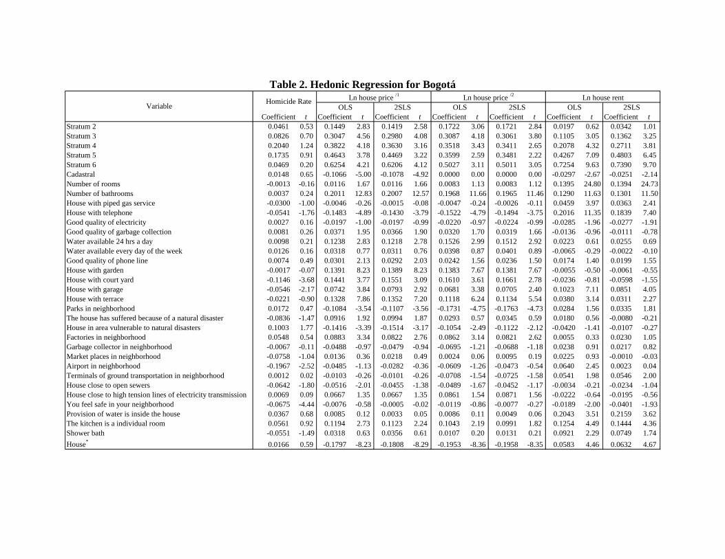
Table 2. Hedonic Regression for Bogotá /1

Coefficient t Coefficient t Coefficient t Coefficient t Coefficient t Coefficient t Coefficient tStratum 2 0.0461 0.53 0.1449 2.83 0.1419 2.58 0.1722 3.06 0.1721 2.84 0.0197 0.62 0.0342 1.01Stratum 3 0.0826 0.70 0.3047 4.56 0.2980 4.08 0.3087 4.18 0.3061 3.80 0.1105 3.05 0.1362 3.25Stratum 4 0.2040 1.24 0.3822 4.18 0.3630 3.16 0.3518 3.43 0.3411 2.65 0.2078 4.32 0.2711 3.81Stratum 5 0.1735 0.91 0.4643 3.78 0.4469 3.22 0.3599 2.59 0.3481 2.22 0.4267 7.09 0.4803 6.45Stratum 6 0.0469 0.20 0.6254 4.21 0.6206 4.12 0.5027 3.11 0.5011 3.05 0.7254 9.63 0.7390 9.70Cadastral 0.0148 0.65 -0.1066 -5.00 -0.1078 -4.92 0.0000 0.00 0.0000 0.00 -0.0297 -2.67 -0.0251 -2.14Number of rooms -0.0013 -0.16 0.0116 1.67 0.0116 1.66 0.0083 1.13 0.0083 1.12 0.1395 24.80 0.1394 24.73Number of bathrooms 0.0037 0.24 0.2011 12.83 0.2007 12.57 0.1968 11.66 0.1965 11.46 0.1290 11.63 0.1301 11.50House with piped gas service -0.0300 -1.00 -0.0046 -0.26 -0.0015 -0.08 -0.0047 -0.24 -0.0026 -0.11 0.0459 3.97 0.0363 2.41House with telephone -0.0541 -1.76 -0.1483 -4.89 -0.1430 -3.79 -0.1522 -4.79 -0.1494 -3.75 0.2016 11.35 0.1839 7.40Good quality of electricity 0.0027 0.16 -0.0197 -1.00 -0.0197 -0.99 -0.0220 -0.97 -0.0224 -0.99 -0.0285 -1.96 -0.0277 -1.91Good quality of garbage collection 0.0081 0.26 0.0371 1.95 0.0366 1.90 0.0320 1.70 0.0319 1.66 -0.0136 -0.96 -0.0111 -0.78Water available 24 hrs a day 0.0098 0.21 0.1238 2.83 0.1218 2.78 0.1526 2.99 0.1512 2.92 0.0223 0.61 0.0255 0.69Water available every day of the week 0.0126 0.16 0.0318 0.77 0.0311 0.76 0.0398 0.87 0.0401 0.89 -0.0065 -0.29 -0.0022 -0.10Good quality of phone line 0.0074 0.49 0.0301 2.13 0.0292 2.03 0.0242 1.56 0.0236 1.50 0.0174 1.40 0.0199 1.55House with garden -0.0017 -0.07 0.1391 8.23 0.1389 8.23 0.1383 7.67 0.1381 7.67 -0.0055 -0.50 -0.0061 -0.55House with court yard -0.1146 -3.68 0.1441 3.77 0.1551 3.09 0.1610 3.61 0.1661 2.78 -0.0236 -0.81 -0.0598 -1.55House with garage -0.0546 -2.17 0.0742 3.84 0.0793 2.92 0.0681 3.38 0.0705 2.40 0.1023 7.11 0.0851 4.05House with terrace -0.0221 -0.90 0.1328 7.86 0.1352 7.20 0.1118 6.24 0.1134 5.54 0.0380 3.14 0.0311 2.27Parks in neighborhood 0.0172 0.47 -0.1084 -3.54 -0.1107 -3.56 -0.1731 -4.75 -0.1763 -4.73 0.0284 1.56 0.0335 1.81The house has suffered because of a natural disaster -0.0836 -1.47 0.0916 1.92 0.0994 1.87 0.0293 0.57 0.0345 0.59 0.0180 0.56 -0.0080 -0.21House in area vulnerable to natural disasters 0.1003 1.77 -0.1416 -3.39 -0.1514 -3.17 -0.1054 -2.49 -0.1122 -2.12 -0.0420 -1.41 -0.0107 -0.27Factories in neighborhood 0.0548 0.54 0.0883 3.34 0.0822 2.76 0.0862 3.14 0.0821 2.62 0.0055 0.33 0.0230 1.05Garbage collector in neighborhood -0.0067 -0.11 -0.0488 -0.97 -0.0479 -0.94 -0.0695 -1.21 -0.0688 -1.18 0.0238 0.91 0.0217 0.82Market places in neighborhood -0.0758 -1.04 0.0136 0.36 0.0218 0.49 0.0024 0.06 0.0095 0.19 0.0225 0.93 -0.0010 -0.03Airport in neighborhood -0.1967 -2.52 -0.0485 -1.13 -0.0282 -0.36 -0.0609 -1.26 -0.0473 -0.54 0.0640 2.45 0.0023 0.04Terminals of ground transportation in neighborhood 0.0012 0.02 -0.0103 -0.26 -0.0101 -0.26 -0.0708 -1.54 -0.0725 -1.58 0.0541 1.98 0.0546 2.00House close to open sewers -0.0642 -1.80 -0.0516 -2.01 -0.0455 -1.38 -0.0489 -1.67 -0.0452 -1.17 -0.0034 -0.21 -0.0234 -1.04House close to high tension lines of electricity transmission 0.0069 0.09 0.0667 1.35 0.0667 1.35 0.0861 1.54 0.0871 1.56 -0.0222 -0.64 -0.0195 -0.56You feel safe in your neighborhood -0.0675 -4.44 -0.0076 -0.58 -0.0005 -0.02 -0.0119 -0.86 -0.0077 -0.27 -0.0189 -2.00 -0.0401 -1.93Provision of water is inside the house 0.0367 0.68 0.0085 0.12 0.0033 0.05 0.0086 0.11 0.0049 0.06 0.2043 3.51 0.2159 3.62The kitchen is a individual room 0.0561 0.92 0.1194 2.73 0.1123 2.24 0.1043 2.19 0.0991 1.82 0.1254 4.49 0.1444 4.36Shower bath -0.0551 -1.49 0.0318 0.63 0.0356 0.61 0.0107 0.20 0.0131 0.21 0.0921 2.29 0.0749 1.74House* 0.0166 0.59 -0.1797 -8.23 -0.1808 -8.29 -0.1953 -8.36 -0.1958 -8.35 0.0583 4.46 0.0632 4.67

Variable Homicide Rate Ln house price Ln house price /2 Ln house rent2SLSOLS 2SLSOLS2SLSOLS

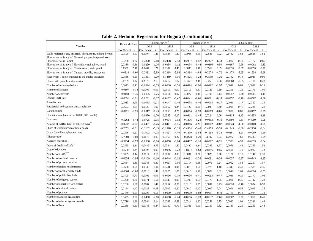
Table 2. Hedonic Regression for Bogotá (Continuation)

Coefficient t Coefficient t Coefficient t Coefficient t Coefficient t Coefficient t Coefficient tWalls material is any of: Brick, block, stone, polished wood 0,0599 1,07 0,1004 1,41 0,0925 1,27 0,0908 1,01 0,0841 0,92 0,1432 3,61 0,1626 3,82Floor material is any of: Marmol, parque, lacquered woodFloor material is Carpet 0,0268 0,77 -0,2370 -7,68 -0,2408 -7,58 -0,2397 -6,57 -0,2427 -6,48 0,0097 0,49 0,0177 0,85Floor material is any of: Floor tile, vinyl, tablet, wood 0,0330 0,86 -0,0290 -1,06 -0,0334 -1,12 -0,0134 -0,44 -0,0166 -0,50 -0,0167 -0,98 -0,0063 -0,33Floor material is any of: Coarse wood, table, plank 0,1531 2,47 0,0487 1,21 0,0307 0,45 0,0638 1,47 0,0519 0,69 -0,0835 -3,07 -0,0355 -0,72Floor material is any of: Cement, gravilla, earth, sand -0,0218 -0,60 -0,2331 -5,99 -0,2318 -5,84 -0,2084 -4,84 -0,2078 -4,72 -0,1473 -5,65 -0,1538 -5,68House with Toilet connected to the public sewerage 0,0886 0,69 -0,1361 -1,09 -0,1489 -1,16 -0,1925 -1,24 -0,2009 -1,26 0,0742 0,74 0,1015 0,99House with potable water service 0,1759 1,22 0,2373 2,13 0,2212 1,72 0,3368 2,41 0,3253 2,06 -0,0368 -0,55 0,0188 0,22Number of infantile shelters ♣ 0,0073 0,12 -0,0594 -1,75 -0,0600 -1,76 -0,0994 -1,96 -0,0992 -1,97 0,0019 0,09 0,0042 0,21Number of asylums ♣ -0,0107 -0,18 0,0009 0,03 0,0019 0,07 0,0116 0,37 0,0123 0,39 0,0209 1,25 0,0175 1,05Number of convents ♣ -0,0459 -1,35 -0,0035 -0,25 0,0014 0,07 0,0072 0,40 0,0108 0,43 -0,0057 -0,78 -0,0201 -1,41Objects theft rate ♣ -0,0991 -1,21 -0,0281 -1,37 -0,0182 -0,47 -0,0141 -0,66 -0,0081 -0,18 -0,0252 -3,10 -0,0562 -1,96Assaults rate ♣ 0,0913 3,95 -0,0053 -0,71 -0,0147 -0,46 -0,0035 -0,46 -0,0095 -0,27 0,0035 1,17 0,0322 1,29Residential and commercial assault rate ♣ 0,0693 1,51 0,0129 1,00 0,0062 0,24 0,0127 0,90 0,0089 0,30 0,0020 0,45 0,0236 1,20Cars theft rate ♣ -0,0721 -2,75 -0,0017 -0,23 0,0056 0,21 -0,0064 -0,70 -0,0019 -0,06 0,0030 0,88 -0,0197 -0,99Homicide rate (deaths per 10'000,000 people) ♣ -0,0470 -1,70 0,0555 0,17 -0,0411 -1,45 0,0224 0,06 -0,0115 -1,43 -0,3253 -1,18Land use ♣ -0,5262 -0,44 -0,0725 -0,15 -0,0094 -0,02 -0,1376 -0,28 -0,0813 -0,16 -0,2480 -0,61 -0,4099 -0,95Attacks of FARC, ELN or other groups** ♣ -0,0237 -0,31 -0,0461 -1,26 -0,0441 -1,15 -0,0366 -0,91 -0,0362 -0,87 -0,0324 -1,60 -0,0400 -1,91Share of women heads of households ♣ -0,2071 -0,21 -2,2102 -5,45 -2,1998 -5,33 -2,4374 -5,40 -2,4475 -5,33 -0,1445 -0,60 -0,2130 -0,84Labor force Unemployment rate ♣ 0,0296 0,57 -0,1002 -4,75 -0,1037 -4,40 -0,1260 -5,84 -0,1288 -5,33 -0,0161 -1,61 -0,0069 -0,50Illiteracy rate ♣ -5,7389 -1,80 0,0479 0,03 0,6566 0,27 -0,3278 -0,20 0,1107 0,04 1,2972 1,69 -0,5061 -0,29Average education ♣ -0,3234 -2,73 -0,0380 -0,96 -0,0050 -0,04 -0,0497 -1,10 -0,0282 -0,21 0,0983 4,95 -0,0035 -0,04Index of Quality of Life*** ♣ 0,0565 2,11 0,0442 4,75 0,0384 1,80 0,0440 4,14 0,0399 1,67 0,0076 1,42 0,0253 1,52Gini of education ♣ 11,0243 1,44 0,2304 0,09 -0,9956 -0,22 -1,8934 -0,63 -2,8396 -0,55 2,8591 1,70 6,3087 1,73Number of CAIS**** ♣ 0,0065 0,14 0,0014 0,10 0,0004 0,03 0,0037 0,27 0,0028 0,20 0,0127 2,10 0,0147 2,30Number of medical centers ♣ -0,0655 -2,95 -0,0109 -1,10 -0,0044 -0,18 -0,0131 -1,26 -0,0091 -0,34 -0,0037 -0,87 -0,0243 -1,35Number of private hospitals ♣ 0,0654 1,89 0,0048 0,30 -0,0017 -0,06 0,0114 0,58 0,0076 0,24 0,0092 1,53 0,0297 1,57Number of police headquarters ♣ 0,0688 0,58 0,0543 1,04 0,0481 0,91 0,0818 1,50 0,0778 1,40 0,0313 2,48 0,0529 2,36Number of local security funds ♣ -0,0064 -1,80 0,0018 1,41 0,0025 1,06 0,0018 1,26 0,0022 0,81 0,0010 1,61 -0,0010 -0,53Number of public hospitals ♣ 0,0405 0,71 0,0008 0,06 -0,0036 -0,19 -0,0056 -0,41 -0,0093 -0,47 0,0016 0,20 0,0142 1,02Number of religious centers ♣ 0,0288 0,76 0,0171 1,56 0,0145 0,93 0,0195 1,65 0,0178 1,05 0,0021 0,45 0,0112 1,22Number of social welfare centers ♣ 0,0266 1,67 0,0084 1,41 0,0054 0,50 0,0110 1,55 0,0091 0,73 -0,0010 -0,40 0,0074 0,97Number of cultural centers ♣ 0,0124 1,47 0,0023 0,98 0,0009 0,20 0,0010 0,42 0,0002 0,04 0,0006 0,56 0,0045 1,26Number of prisons ♣ 0,2469 0,91 0,0203 0,51 -0,0079 -0,09 -0,0009 -0,02 -0,0201 -0,19 0,0168 0,73 0,0944 1,31Number of attacks against life ♣ 0,0425 0,80 -0,0460 -2,60 -0,0508 -2,24 -0,0606 -3,23 -0,0637 -2,61 -0,0067 -0,72 0,0068 0,45Number of attacks against wealth ♣ 0,0716 1,26 0,0344 2,14 0,0262 0,88 0,0314 1,82 0,0251 0,75 0,0092 1,04 0,0316 1,49Number of bars ♣ 0,0285 0,51 0,0148 0,84 0,0130 0,71 0,0161 0,91 0,0159 0,82 0,0180 2,29 0,0269 2,48

Ln house price /2 Ln house rentOLS 2SLS OLS 2SLS OLS 2SLSVariable Homicide Rate Ln house price /1

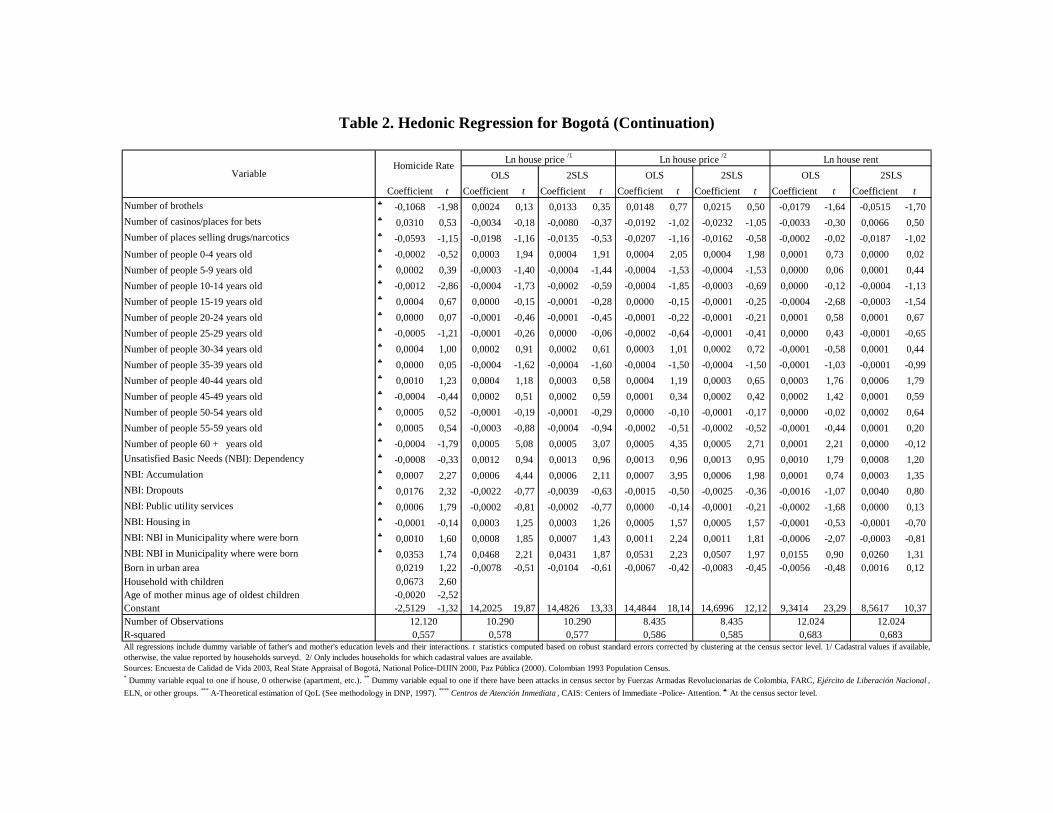
Coefficient t Coefficient t Coefficient t Coefficient t Coefficient t Coefficient t Coefficient tNumber of brothels ♣ -0,1068 -1,98 0,0024 0,13 0,0133 0,35 0,0148 0,77 0,0215 0,50 -0,0179 -1,64 -0,0515 -1,70Number of casinos/places for bets ♣ 0,0310 0,53 -0,0034 -0,18 -0,0080 -0,37 -0,0192 -1,02 -0,0232 -1,05 -0,0033 -0,30 0,0066 0,50Number of places selling drugs/narcotics ♣ -0,0593 -1,15 -0,0198 -1,16 -0,0135 -0,53 -0,0207 -1,16 -0,0162 -0,58 -0,0002 -0,02 -0,0187 -1,02Number of people 0-4 years old ♣ -0,0002 -0,52 0,0003 1,94 0,0004 1,91 0,0004 2,05 0,0004 1,98 0,0001 0,73 0,0000 0,02Number of people 5-9 years old ♣ 0,0002 0,39 -0,0003 -1,40 -0,0004 -1,44 -0,0004 -1,53 -0,0004 -1,53 0,0000 0,06 0,0001 0,44Number of people 10-14 years old ♣ -0,0012 -2,86 -0,0004 -1,73 -0,0002 -0,59 -0,0004 -1,85 -0,0003 -0,69 0,0000 -0,12 -0,0004 -1,13Number of people 15-19 years old ♣ 0,0004 0,67 0,0000 -0,15 -0,0001 -0,28 0,0000 -0,15 -0,0001 -0,25 -0,0004 -2,68 -0,0003 -1,54Number of people 20-24 years old ♣ 0,0000 0,07 -0,0001 -0,46 -0,0001 -0,45 -0,0001 -0,22 -0,0001 -0,21 0,0001 0,58 0,0001 0,67Number of people 25-29 years old ♣ -0,0005 -1,21 -0,0001 -0,26 0,0000 -0,06 -0,0002 -0,64 -0,0001 -0,41 0,0000 0,43 -0,0001 -0,65Number of people 30-34 years old ♣ 0,0004 1,00 0,0002 0,91 0,0002 0,61 0,0003 1,01 0,0002 0,72 -0,0001 -0,58 0,0001 0,44Number of people 35-39 years old ♣ 0,0000 0,05 -0,0004 -1,62 -0,0004 -1,60 -0,0004 -1,50 -0,0004 -1,50 -0,0001 -1,03 -0,0001 -0,99Number of people 40-44 years old ♣ 0,0010 1,23 0,0004 1,18 0,0003 0,58 0,0004 1,19 0,0003 0,65 0,0003 1,76 0,0006 1,79Number of people 45-49 years old ♣ -0,0004 -0,44 0,0002 0,51 0,0002 0,59 0,0001 0,34 0,0002 0,42 0,0002 1,42 0,0001 0,59Number of people 50-54 years old ♣ 0,0005 0,52 -0,0001 -0,19 -0,0001 -0,29 0,0000 -0,10 -0,0001 -0,17 0,0000 -0,02 0,0002 0,64Number of people 55-59 years old ♣ 0,0005 0,54 -0,0003 -0,88 -0,0004 -0,94 -0,0002 -0,51 -0,0002 -0,52 -0,0001 -0,44 0,0001 0,20Number of people 60 + years old ♣ -0,0004 -1,79 0,0005 5,08 0,0005 3,07 0,0005 4,35 0,0005 2,71 0,0001 2,21 0,0000 -0,12Unsatisfied Basic Needs (NBI): Dependency ♣ -0,0008 -0,33 0,0012 0,94 0,0013 0,96 0,0013 0,96 0,0013 0,95 0,0010 1,79 0,0008 1,20NBI: Accumulation ♣ 0,0007 2,27 0,0006 4,44 0,0006 2,11 0,0007 3,95 0,0006 1,98 0,0001 0,74 0,0003 1,35NBI: Dropouts ♣ 0,0176 2,32 -0,0022 -0,77 -0,0039 -0,63 -0,0015 -0,50 -0,0025 -0,36 -0,0016 -1,07 0,0040 0,80NBI: Public utility services ♣ 0,0006 1,79 -0,0002 -0,81 -0,0002 -0,77 0,0000 -0,14 -0,0001 -0,21 -0,0002 -1,68 0,0000 0,13NBI: Housing in ♣ -0,0001 -0,14 0,0003 1,25 0,0003 1,26 0,0005 1,57 0,0005 1,57 -0,0001 -0,53 -0,0001 -0,70NBI: NBI in Municipality where were born ♣ 0,0010 1,60 0,0008 1,85 0,0007 1,43 0,0011 2,24 0,0011 1,81 -0,0006 -2,07 -0,0003 -0,81NBI: NBI in Municipality where were born ♣ 0,0353 1,74 0,0468 2,21 0,0431 1,87 0,0531 2,23 0,0507 1,97 0,0155 0,90 0,0260 1,31Born in urban area 0,0219 1,22 -0,0078 -0,51 -0,0104 -0,61 -0,0067 -0,42 -0,0083 -0,45 -0,0056 -0,48 0,0016 0,12Household with children 0,0673 2,60Age of mother minus age of oldest children -0,0020 -2,52Constant -2,5129 -1,32 14,2025 19,87 14,4826 13,33 14,4844 18,14 14,6996 12,12 9,3414 23,29 8,5617 10,37Number of ObservationsR-squared

Ln house price /2 Ln house rentOLS 2SLS OLS 2SLS OLS 2SLSVariable

Homicide Rate Ln house price /1

All regressions include dummy variable of father's and mother's education levels and their interactions. t statistics computed based on robust standard errors corrected by clustering at the census sector level. 1/ Cadastral values if available,otherwise, the value reported by households surveyd. 2/ Only includes households for which cadastral values are available.Sources: Encuesta de Calidad de Vida 2003, Real State Appraisal of Bogotá, National Police-DIJIN 2000, Paz Pública (2000). Colombian 1993 Population Census.* Dummy variable equal to one if house, 0 otherwise (apartment, etc.). ** Dummy variable equal to one if there have been attacks in census sector by Fuerzas Armadas Revolucionarias de Colombia, FARC, Ejército de Liberación Nacional , ELN, or other groups. *** A-Theoretical estimation of QoL (See methodology in DNP, 1997). **** Centros de Atención Inmediata , CAIS: Centers of Immediate -Police- Attention. ♣ At the census sector level.

0,6838.435 12.02412.024

0,6830,557 0,5770,578 0,5850,58612.120 10.29010.290 8.435

Table 2. Hedonic Regression for Bogotá (Continuation)

Table 3 presents the results of instrumenting the homicide rate with the previously defined age difference, as well as a dummy variable equal to one if the household has at least one children living in the house, and zero otherwise. The first column presents the first stage results, in which we can see that our instruments are statistically significant, and the age difference has the expected negative sign. Once we focus on the homicide rate, we find that while in the first regression (cadastral and reported house values) the coefficient of the interactions between the homicide rate and strata 3 and 6 were formerly positive, once we instrument, only the coefficients of the homicide rate and strata 5 and 6 become significant and negative. When we use only cadastral data, the interaction with socioeconomic strata which were not being statistically significant, become significant and negative for stratum 6, and weakly significant for stratum 5. Finally, result for rent values that in the case of the interaction with socioeconomic strata was positive and significant for stratum 6, becomes non significant. The final 2SLS result implies an elasticity of 1%, or that if the homicide rate in stratum 6 is increased by one standard deviation, from a mean of 0.009 to 0.074 (that is, an increase to 7.3 times the mean), the values of the house would fall 7.2%. In the case of stratum 5, the elasticity of 2% would imply a fall of 2.4% in the value of the house. On the other hand, the objects theft, assaults, and residential and commercial assaults rates, the attacks of guerilla groups, and the attacks against wealth are not significant. The cars theft rate becomes negative and significant only for its interaction with stratum 5. Finally, the attacks against life keep being negative and statistically significant.

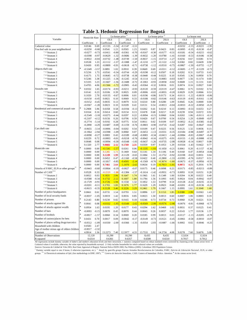
Table 3. Hedonic Regression for Bogotá

Coefficient t Coefficient t Coefficient t Coefficient t Coefficient t Coefficient t Coefficient tCadastral value 0.0146 0.69 -0.1135 -5.54 -0.1147 -5.51 -0.0232 -2.15 -0.0221 -1.95You feel safe in your neighborhood -0.0250 -0.68 0.0541 1.21 0.0565 1.23 0.0433 0.87 0.0423 0.83 -0.0095 -0.35 -0.0130 -0.47

" * Stratum 2 -0.0277 -0.73 -0.0411 -0.80 -0.0361 -0.70 -0.0167 -0.30 -0.0177 -0.31 -0.0181 -0.54 -0.0215 -0.62" * Stratum 3 -0.0398 -0.97 -0.0629 -1.32 -0.0686 -1.39 -0.0632 -1.20 -0.0780 -1.41 -0.0160 -0.53 -0.0186 -0.58" * Stratum 4 -0.0022 -0.04 -0.0732 -1.48 -0.0749 -1.50 -0.0637 -1.15 -0.0714 -1.27 0.0256 0.67 0.0281 0.74" * Stratum 5 0.0538 1.23 -0.1112 -1.57 -0.1088 -1.47 -0.1210 -1.77 -0.1122 -1.53 0.0382 0.82 0.0439 0.90" * Stratum 6 0.0430 0.95 -0.0809 -0.91 -0.0618 -0.71 -0.0738 -1.12 -0.0510 -0.75 -0.0867 -1.50 -0.0755 -1.27

Objects theft rate ♣ -0.5349 -3.57 0.0891 1.02 0.0910 0.39 0.0669 0.69 -0.0311 -0.12 -0.0695 -1.77 -0.1229 -0.72" * Stratum 2 0.5236 1.73 -0.0541 -0.34 -0.0744 -0.29 -0.0198 -0.12 0.0507 0.18 0.0202 0.31 0.0733 0.43" * Stratum 3 0.4175 1.75 -0.0645 -0.72 -0.0738 -0.38 -0.0440 -0.44 0.0225 0.10 0.0545 1.36 0.0950 0.70" * Stratum 4 0.5246 3.38 -0.1225 -1.36 -0.1245 -0.54 -0.1114 -1.13 -0.0083 -0.03 0.0677 1.56 0.1174 0.69" * Stratum 5 0.5335 3.23 -0.1667 -1.56 -0.1688 -0.72 -0.1063 -0.93 -0.0058 -0.02 0.0608 1.15 0.1131 0.65" * Stratum 6 0.4705 4.06 -0.1566 -1.72 -0.0905 -0.43 -0.0364 -0.32 0.0016 0.01 0.0074 0.16 0.0927 0.60

Assaults rate ♣ 0.0332 1.65 -0.0174 -0.93 -0.0211 -0.93 -0.0120 -0.59 -0.0119 -0.47 0.0061 0.75 0.0102 0.74" * Stratum 2 0.0141 0.23 0.0106 0.39 0.0025 0.09 -0.0006 -0.02 -0.0055 -0.20 0.0029 0.29 0.0066 0.53" * Stratum 3 0.1020 2.70 -0.0135 -0.67 0.0006 0.01 -0.0196 -0.86 0.0173 0.34 -0.0111 -1.22 -0.0019 -0.06" * Stratum 4 -0.0150 -0.45 0.0021 0.10 0.0069 0.33 -0.0188 -0.82 -0.0146 -0.63 -0.0119 -0.95 -0.0161 -1.18" * Stratum 5 -0.0152 -0.45 0.0035 0.13 0.0079 0.33 0.0210 0.80 0.0280 1.09 0.0045 0.26 0.0000 0.00" * Stratum 6 -0.0367 -1.28 0.0023 0.10 0.0109 0.41 0.0131 0.54 -0.0013 -0.04 -0.0033 -0.22 -0.0050 -0.23

Residential and commercial assault rate ♣ 0.2908 5.96 0.0358 0.58 -0.0194 -0.13 0.0262 0.41 0.0210 0.13 -0.0093 -0.53 0.0253 0.27" * Stratum 2 0.0164 0.16 0.0414 0.60 0.0134 0.13 0.0478 0.68 0.0217 0.20 0.0239 0.94 0.0372 0.91" * Stratum 3 -0.2549 -3.18 -0.0275 -0.44 0.0297 0.22 -0.0094 -0.15 0.0060 0.04 0.0202 1.06 -0.0111 -0.13" * Stratum 4 -0.2107 -4.12 0.0156 0.26 0.0706 0.59 0.0420 0.67 0.0700 0.54 0.0254 1.29 -0.0049 -0.07" * Stratum 5 -0.2774 -5.14 0.0192 0.28 0.0775 0.54 0.0011 0.02 0.0109 0.07 -0.0052 -0.21 -0.0385 -0.42" * Stratum 6 -0.2890 -4.29 -0.0487 -0.69 -0.1159 -0.76 -0.0803 -0.90 -0.0716 -0.42 0.0287 0.82 -0.0647 -0.63

Cars theft rate ♣ -0.0655 -3.14 -0.0006 -0.04 0.0202 0.54 0.0109 0.47 0.0225 0.56 0.0125 1.32 0.0036 0.15" * Stratum 2 -0.1964 -2.94 -0.0398 -1.09 0.0060 0.07 -0.0453 -1.13 -0.0331 -0.35 -0.0184 -0.98 -0.0497 -0.77" * Stratum 3 -0.0098 -0.27 0.0083 0.43 -0.0189 -0.68 -0.0083 -0.34 -0.0413 -1.44 -0.0084 -0.83 -0.0067 -0.46" * Stratum 4 0.0229 0.72 -0.0003 -0.01 -0.0218 -0.76 -0.0042 -0.16 -0.0275 -0.91 -0.0155 -1.20 -0.0088 -0.52" * Stratum 5 0.0048 0.08 -0.0094 -0.30 -0.0348 -1.05 -0.0437 -1.26 -0.0735 -2.08 -0.0028 -0.14 0.0017 0.08" * Stratum 6 0.1320 2.77 0.0602 2.12 0.1769 2.31

0.1249 1.99

0.7461 2.64 0.9072 4.25

0.0359 0.97 0.1053 1.29 -0.0334 -1.43 0.0422 0.77Homicide rate ♣ 0.0000 0.00 -0.1541 -2.57 0.0261 0.06 -0.1335 -1.93 -0.1050 -0.21 0.0061 0.20 -0.1157 -0.36

" * Stratum 2 0.0000 0.00 0.1281 1.71 0.1469 0.64 0.1141 1.34 0.1106 0.44 0.0160 0.47 -0.0054 -0.06" * Stratum 3 0.0000 0.00 -0.1129 -0.65 0.1084 1.53 -0.1752 -0.92 -0.0198 -0.63 0.0031 0.04" * Stratum 4 0.0000 0.00 0.0452 0.47 -0.1160 -0.58 0.0422 0.40 -0.2800 -1.33 -0.0395 -0.76 0.0517 0.51" * Stratum 5 0.0000 0.00 -0.1817 -0.85 -0.4501 -2.14 -0.1569 -0.76 -0.3674 -1.60 -0.0673 -0.37 -0.0956 -0.55" * Stratum 6 0.0000 0.00 -1.1070 -2.63 0.0634 0.19 -0.7913 -1.91 0.2016 0.78

Attacks of FARC, ELN or other groups** ♣ -0.0443 -0.60 -0.0064 -0.19 -0.0027 -0.07 0.0175 0.46 0.0098 0.23 -0.0171 -0.85 -0.0213 -0.89Number of CAIS**** 0.0528 0.33 -0.1519 -1.88 -0.1384 -1.57 -0.1614 -1.42 -0.0931 -0.73 0.0093 0.18 0.0151 0.28

" * Stratum 2 0.0052 0.03 0.1831 2.06 0.1647 1.74 0.1965 1.61 0.1349 1.00 0.0204 0.38 0.0222 0.40" * Stratum 3 -0.0588 -0.34 0.1732 2.12 0.1607 1.80 0.1784 1.56 0.1093 0.85 0.0024 0.04 -0.0042 -0.07" * Stratum 4 -0.1729 -0.91 0.1726 1.94 0.1558 1.32 0.1852 1.53 0.0799 0.54 -0.0128 -0.22 -0.0235 -0.31" * Stratum 5 -0.0201 -0.11 0.1765 1.83 0.1676 1.77 0.1629 1.29 0.0923 0.68 -0.0201 -0.33 -0.0136 -0.22" * Stratum 6 -0.0615 -0.35 0.3128 3.46 0.3226 3.29 0.2461 1.79 0.1667 1.15 0.0995 1.61 0.1040 1.68

Number of police headquarters ♣ 0.0661 0.61 0.0731 1.54 0.0793 1.51 0.0896 1.57 0.1153 1.85 0.0380 2.99 0.0363 1.43Number of local security funds ♣ -0.0037 -1.05 0.0019 1.42 0.0016 0.85 0.0023 1.50 0.0013 0.60 0.0007 1.06 0.0003 0.19Number of prisons ♣ 0.2143 0.80 0.0230 0.82 0.0165 0.18 0.0246 0.73 0.0734 0.73 0.0060 0.28 0.0221 0.31Number of attacks against life ♣ 0.0041 0.08 -0.0332 -1.95 -0.0349 -2.02 -0.0569 -2.99 -0.0576 -2.98 -0.0076 -0.81 -0.0068 -0.73Number of attacks against wealth ♣ 0.0954 1.63 0.0195 1.20 0.0177 0.43 0.0294 1.62 0.0469 1.02 0.0031 0.37 0.0125 0.41Number of bars ♣ -0.0093 -0.15 0.0070 0.45 0.0070 0.44 0.0043 0.26 0.0037 0.22 0.0143 1.77 0.0136 1.57Number of brothels ♣ -0.0817 -1.57 0.0060 0.34 0.0069 0.20 0.0185 0.99 0.0013 0.03 -0.0117 -1.13 -0.0205 -0.78Number of casinos/places for bets ♣ 0.0431 0.70 0.0017 0.09 -0.0042 -0.17 -0.0149 -0.73 -0.0121 -0.45 -0.0061 -0.58 -0.0010 -0.07Number of places selling drugs/narcotics ♣ -0.0512 -1.09 -0.0330 -2.00 -0.0366 -1.35 -0.0354 -2.03 -0.0487 -1.66 0.0002 0.02 -0.0046 -0.25Household with children 0.0583 2.47Age of mother minus age of oldest children -0.0017 -2.32Constant 4.9914 1.56 13.2273 7.40 12.5977 4.33 13.7531 5.92 14.2756 4.08 9.0278 7.60 9.6076 5.08Number of ObservationsR-squared 0.7017

Variable Homicide Rate Ln house price /1 Ln house price /2 Ln house rent

0.65108,4350.6508

12,0240.70120.6314

10,2900.6357

10,2900.6361

OLS 2SLSOLS

12,120 8,435 12,024

2SLSOLS 2SLS

All regressions include dummy variable of father's and mother's education levels and their iteractions. t statistics computed based on robust standard errors corrected by clustering at the census sector level. 1/Cadastral values if available, otherwise, the value reported by households surveyd. 2/ Only includes households for which cadastral values are available.Sources: Encuesta de Calidad de Vida 2003, Real State Appraisal of Bogotá, National Police-DIJIN 2000, Paz Pública (2000). Colombian 1993 Population Census.* Dummy variable equal to one if house, 0 otherwise (apartment, etc.). ** Attack by guerrilla groups Fuerzas Armadas Revolucionarias de Colombia, FARC, Ejército de Liberación Nacional , ELN, or othergroups. *** A-Theoretical estimation of QoL (See methodology in DNP, 1997). **** Centros de Atención Inmediata , CAIS: Centers of Immediate -Police- Attention. ♣ At the census sector level.

Conclusions In this paper we use hedonic price models to estimate the value households are willing to pay to avoid crime, and in particular, high homicides rates, in Bogotá. We and find that households living in the highest socioeconomic stratum, stratum 6, are paying up to 7.2% of their house values to keep their average homicide rates and avoid increasing them in one standard deviation. On their part, households in strata 5, that with the next group of richest population in the city, would be paying up to 2.4% of their house values to keep their average homicide rates. The result reveals the willingness to pay for security by households in Bogotá, and additionally, reveals that a supposed pure public good like security, ends up propitiating urban private markets that auction security. These markets imply different levels of access to public goods among the population, and actually, the exclusion of the poorest. We find as well evidence of negative capitalization of the rate of attacks against life, and positive capitalization of the presence of police authority in the form of Centers of Immediate Attention, CAIS.

References Atkinson, Giles; Healey, Andrew, and Mourato, Susan (2005) “Valuing the Costs of

Violent Crime: A Stated Preference Approach” Oxford Economic Papers 57, 559-585. Oxford University Press

Ansellin L. (1988) “Spatial Econometrics Methods and Models” Klwer Academics Publisher, University of California, Santa Barbara.

Badel, Martha (1999) “La Violencia de los Años Noventa en Colombia: Su Evolución en las Grandes Ciudades y Costos Económicos Directos” Informe de Consultoría DNP-UPRU, Santafé de Bogotá D.C.

Bogotá (2004) “Diagnóstico físico y socioeconómico de las localidades de Bogotá, D.C.” there is one document per localidad. Download

Blomquist, G.C.; Berger, M.C. and Hoehn, J.P. (1988) “New Estimates of Quality of Life in Urban Areas”, American Economic Review, 78, pp.89-107.

Castaño, Elkin (2006) “Condiciones de Vida en la Ciudad de Medellín” Planeación Metropolitana – Centro de Estudios de Opinión, Universidad de Antioquia

Cohen, Mark; Rust, Roland; Oteen, Sara, and Tidd, Simon T. (2004) “Willingness to Pay For Crime Control Programs” Criminology, February.

Conley, Timothy G. and Topa, Giorgio (2002) “Socio-Economic Distance and Spatial Patterns in Unemployment”, Journal of Applied Econometrics, Vol. 17, 2002, 303-327.

Cook, Philip J., and Ludwig, Jens (2000) “Gun Violence: The Real Costs” New York: Oxford University Press.

Departamento Nacional de Planeación, DNP (1997) “Índice de Condiciones de Vida Urbano-Rural” Misión Social.

Donohue, John J. and Levitt, Steven D. (2000) “The Impact of Legalized Abortion on Crime” NBER WP 8004

Fajnzylber, Pablo; Lederman, Daniel, and Loayza, Norman (2002a) “What Causes Violent Crime?”, European Economic Review, Vol. 46, pp. 1323-1357.

Fajnzylber, Pablo; Lederman, Daniel, and Loayza, Norman (2002b) “Inequality and Violent Crime”, Journal of Law and Economics, Vol. XLV, (April), pp. 1-40.

Fajnzylber, Pablo; Lederman, Daniel, and Loayza, Norman (2000) “Crime and Victimization: An Economic Perspective”, Economia, Vol. 1 (1), pp. 219-278.

Fajnzylber, Pablo; Lederman, Daniel, and Loayza, Norman (1998) “Determinants of Crime Rates in Latin America and the World: An Empirical Assessment”, The World Bank, Washington DC.

Farrington DP (1998) “Predictors, Causes, and Correlates of Male Youth Violence” In: Tonry M, Moore MH, eds. Youth Violence. Chicago, IL, University of Chicago Press: 421–475.

Flórez, Carmen E. (2007) “Demographics and Poverty in Colombia” Poverty Mission, mimeo

Gaviria, Alejandro, and Pages, Carmen (2000) “Patterns of crime victimization in Latin America” mimeo, Inter American Development Bank (March).

Gavira, Alejandro, and Vélez, Carlos Eduardo (2001) “Who Bears the Burden of Crime in Colombia?” mimeo, Fedesarrollo.

González, J; Fresneda, O.; Martínez, P.; Rodríguez, O.; Sarmiento, A.; Oviedo, M.; Lasso, F.; and Camacho, D. (2004) “Evolución de los Principales Indicadores Sociales de Bogotá (1990-2003)” mimeo, Alcaldía de Bogotá. Download

Gyourko, J.; Kahn, M. and J. Tracy (1999) “Quality of Life and Environmental Comparisons,” Handbook of Regional and Urban Economics, Volume 3, edited by Paul Cheshire and Edwin Mills, 1413-1454. New York, North-Holland, 1999.

Hall, P.; Fisher, N.I., and Hoffman, B. (1994) “On the Non-Parametric Estimation of Covariance Functions” The Annals of Statistics, Vol. 22, No. 4 (December), pp. 2115-2134.

Heinemann, Alessandra and Verner, Dorte (2006) “Crime and Violence in Development: A Literature Review of Latina American and Caribbean” World Bank Policy Research Working Paper 4041, October.

Hunt, Jennifer (2003) “Teen Births Keep American Crime High” NBER WP 9632 Krug, Etienne G.; Dahlberg, Linda L.; Mercy, James A.; Zwi, Anthony B. and Lozano,

Rafael (2002) “World Report on Violence and Health” Geneva, World Health Organization.

Londoño, Juan Luis and Guerrero, Rodrigo (2000) “Violencia en América Latina: Epidemiología y Costos” Banco Interamericano de Desarrollo.

Ludwig, Jens and Cook, Philip J. (2001) “The Benefits of Reducing Gun Violence: Evidence from Contingent-Valuation Curvey Data” Journal of Risk and Uncertainty, 22: 207-26

Llorente, María Victoria; Escobedo, Rodolfo; Echandía, Camilo, and Rubio, Mauricio (2001) “Violencia Homicida en Bogotá: Más que Intolerancia” Documento CEDE 2001-04

Medina, Carlos, and Morales, Leonardo (2006) “Stratification and Public Utility Services in Colombia: Subsidies to Households or Distortions on Housing Prices?” forthcoming in Economia. Download

Medina, Carlos, and Morales, Leonardo, and Núñez, Jairo (2007) “Quality of Life in Urban Neighborhoods: The Case of Bogotá” Proposal to the Research Network of the Research Department, Inter American Development Bank.

Medina, Carlos and Núñez, Jairo (2006) “La Oferta de Servicios del Sector Financiero Formal en Bogotá” Coyuntura Social N° 35, December 2006. Fedesarrollo, pp. 111-129. Download WP

Morales, Leonardo (2006) “La Calidad de la Vivienda en Bogotá: Enfoque de Precios Hedónicos de Hogares y Agregados Espaciales”, Revista Sociedad y Economía 9. Download

Moran P. (1948) “The interpretation of statistical maps”, Journal of the Royal Statistical Society B, 10, 243-251.

Morash M, Rucker L. (1989) “An Exploratory Study of the Connection of Mother’s Age at Childbearing to Her Children’s Delinquency in Four Data Sets” Crime and Delinquency, 35:45–93.

Nagin DS, Pogarsky G, Farrington DP (1997) “Adolescent Mothers and the Criminal Behavior of their Children” Law and Society Review, 31:137–162.

Núñez, Jairo, and Sánchez, Fabio (2001) “Interrelaciones Espaciales en los Delitos Contra el Patrimonio en Bogota” mimeo

Paz Pública (2000) “Escenarios del Crimen en los Barrios y Localidades de Bogotá” Investigación “Caracterización de la Violencia Homicida en Bogotá”, Documento de Trabajo No. 1. Bogotá: Paz Pública-CEDE-UNIANDES and Alcaldía de Bogotá.

Roback, Jennifer (1982) “Wages, Rents, and the Quality of Life” Journal of Political Economy 90: 1257-1278.

Roback, Jennifer (1988) “Wages, Rents, and Amenities: Differences Among Workers and Regions” Economic Inquiry 26 (January): 23-41.

Rosen, Sherwin (1974) “Hedonic Prices and Implicit Markets: Product Differentiation in Pure Competition” Journal of Political Economy 82 (January/February): 34-55.

Rosen, Sherwin (1979) “Wage-based Indexes of Urban Quality of Life” In Current Issues in Urban Economics, edited by Peter Mieszkowski and Mahlon Straszheim. Baltimore, Johns Hopkins University Press.

Sanchez, F. and Nuñez, J. (2000) “Determinantes del Crimen Violento en un País Altamente Violento: el Caso de Colombia.” Mimeo, Universidad de los Andes, Bogotá.

Sherwin Rosen (2002) “Markets and Diversity” The American Economic Review, Vol. 92, No. 1. (Mar., 2002), pp. 1-15.

Topa, Giorgio (2001) “Social Interactions, Local Spillovers and Unemployment”, Review of Economic Studies, Vol. 68 (2), April, 261-295.

United Nations Population Fund, UNFPA (2007) “State of World Population 2007: Unleashing the Potential of Urban Growth”. Download