ISSN 1063-7729, Astronomy Reports, 2007, Vol. 51, No. 9, pp. 709–734. c Pleiades Publishing, Ltd., 2007. Published in Russian in Astronomicheski˘ ı Zhurnal, 2007, Vol. 84, No. 9, pp. 786–815. The Cosmological Mass Function A. Del Popolo 1, 2 and I. S. Yesilyurt 3 1 Bogazici University, Physics Department, 80815 Bebek, Istanbul, Turkey 2 Dipartimento di Matematica, Universit ` a Statale di Bergamo, via dei Caniana 2, 24127, Bergamo, ITALY 3 Kandilli Observatory and Earthquake Research Institute, Bogazici University, 34684, Clengelkoy, Istanbul, Turkey Received April 5, 2007 Abstract—This paper reviews the cosmological mass function from a theoretical point of view, starting from the seminal paper of Press and Shechter to the latest developments, and discusses some improvements on mass-function models in the literature. The numerical mass function given by Yahagi et al. YNY is compared with the theoretical mass function obtained in the present paper by means of an excursion- set model and an improved version of the barrier shape obtained by Del Popolo and Gambera [30], which implicitly takes account of the total angular momentum acquired by the proto-structure during its evolution and of a non-zero cosmological constant. The mass function obtained in the present paper is in better agreement with the simulations of Del Popolo than other previous models. The mass function considered provides as good a fit to the simulation results as the function proposed in Del Popolo, but, in contrast to this latter function, was derived from a sound theoretical basis. The evolution of the mass function is calculated in a ΛCDM model, and the results compared with those of Reed et al. [94], who used a high resolution ΛCDM numerical simulation to calculate the mass function of dark matter haloes down to the scale of dwarf galaxies and back to a redshift of fifteen. The mass function obtained in the present paper gives similar predictions as the Sheth–Tormen (ST) mass function, but does not overpredict the number of extremely rare objects. The results confirm previous findings that the simulated halo mass function can be described solely by the variance of the mass distribution, and thus has no explicit redshift dependence. It is show that a PS-like approach together with the ellipsoidal model introduced in Del Popolo provides a better description of the theoretical mass function. PACS numbers : 98.65.Dx, 98.80.Jk, 98.80.Bp, 95.30.Sf DOI: 10.1134/S1063772907090028 1. INTRODUCTION The observed Universe appears quite clumpy and inhomogeneous on spatial scales of 200 h −1 Mpc. Beyond that scale mass clumps appear to be homoge- neously distributed. We observe massive clumps such as galaxies, groups of galaxies, clusters of galaxies, and super-clusters (the most massive among the hi- erarchy of structures) fill space spanning a wide range of mass scales. The mass ranges characterizing these systems are, respectively 10 9 −10 10 M , 10 11 M , 10 12 −10 14 M , and 10 15 M , where M is the solar mass. All these objects combined form what is known as the Large Scale Structure of the Universe. One of the most fundamental challenges in present astrophysics is to understand the formation and evo- lution of the Large Scale Structure. In order to un- derstand the Large Scale Structure, we need to have a theoretical framework that can make predictions ∗ The text was submitted by the author in English. about structure formation. The leading idea of all structure-formation theories is that structures were born from small perturbations in an otherwise uniform distribution of matter in the early Universe, which is supposed to be, in great part, dark (matter not detectable through light emission). The term Dark Matter indicates a hypothetic material component of the Universe that does not directly emit electromag- netic radiation (unless it decays into particles having this property ([1], but also see [2])). Dark matter cannot be revealed directly, but it is necessary to postulate its existence in order to explain the discrepancies between the observed dynamical properties of galaxies and clusters of galaxies and the- oretical predictions based on models of these objects assuming that the only matter present is the visible matter. The first hypotheses about Dark Matter go back to measurements performed by Oort [3] of the matter surface density in the Galactic disk, obtained by analyzing the motions of stars perpendicular to the 709

Welcome message from author
This document is posted to help you gain knowledge. Please leave a comment to let me know what you think about it! Share it to your friends and learn new things together.
Transcript
ISSN 1063-7729, Astronomy Reports, 2007, Vol. 51, No. 9, pp. 709–734. c© Pleiades Publishing, Ltd., 2007.Published in Russian in Astronomicheskiı Zhurnal, 2007, Vol. 84, No. 9, pp. 786–815.
The Cosmological Mass Function
A. Del Popolo1, 2 and I. S. Yesilyurt3
1Bogazici University, Physics Department, 80815 Bebek, Istanbul, Turkey2Dipartimento di Matematica, Universita Statale di Bergamo,
via dei Caniana 2, 24127, Bergamo, ITALY3Kandilli Observatory and Earthquake Research Institute, Bogazici University,
34684, Clengelkoy, Istanbul, TurkeyReceived April 5, 2007
Abstract—This paper reviews the cosmological mass function from a theoretical point of view, startingfrom the seminal paper of Press and Shechter to the latest developments, and discusses some improvementson mass-function models in the literature. The numerical mass function given by Yahagi et al. YNY iscompared with the theoretical mass function obtained in the present paper by means of an excursion-set model and an improved version of the barrier shape obtained by Del Popolo and Gambera [30], whichimplicitly takes account of the total angular momentum acquired by the proto-structure during its evolutionand of a non-zero cosmological constant. The mass function obtained in the present paper is in betteragreement with the simulations of Del Popolo than other previous models. The mass function consideredprovides as good a fit to the simulation results as the function proposed in Del Popolo, but, in contrastto this latter function, was derived from a sound theoretical basis. The evolution of the mass function iscalculated in a ΛCDM model, and the results compared with those of Reed et al. [94], who used a highresolution ΛCDM numerical simulation to calculate the mass function of dark matter haloes down to thescale of dwarf galaxies and back to a redshift of fifteen. The mass function obtained in the present papergives similar predictions as the Sheth–Tormen (ST) mass function, but does not overpredict the numberof extremely rare objects. The results confirm previous findings that the simulated halo mass function canbe described solely by the variance of the mass distribution, and thus has no explicit redshift dependence.It is show that a PS-like approach together with the ellipsoidal model introduced in Del Popolo provides abetter description of the theoretical mass function.
PACS numbers : 98.65.Dx, 98.80.Jk, 98.80.Bp, 95.30.SfDOI: 10.1134/S1063772907090028
1. INTRODUCTIONThe observed Universe appears quite clumpy and
inhomogeneous on spatial scales of � 200 h−1 Mpc.Beyond that scale mass clumps appear to be homoge-neously distributed. We observe massive clumps suchas galaxies, groups of galaxies, clusters of galaxies,and super-clusters (the most massive among the hi-erarchy of structures) fill space spanning a wide rangeof mass scales. The mass ranges characterizing thesesystems are, respectively �109−1010 M�,�1011 M�,�1012−1014 M�, and �1015 M�, where M� is thesolar mass. All these objects combined form what isknown as the Large Scale Structure of the Universe.One of the most fundamental challenges in presentastrophysics is to understand the formation and evo-lution of the Large Scale Structure. In order to un-derstand the Large Scale Structure, we need to havea theoretical framework that can make predictions
∗The text was submitted by the author in English.
about structure formation. The leading idea of allstructure-formation theories is that structures wereborn from small perturbations in an otherwise uniformdistribution of matter in the early Universe, whichis supposed to be, in great part, dark (matter notdetectable through light emission). The term DarkMatter indicates a hypothetic material component ofthe Universe that does not directly emit electromag-netic radiation (unless it decays into particles havingthis property ([1], but also see [2])).
Dark matter cannot be revealed directly, but it isnecessary to postulate its existence in order to explainthe discrepancies between the observed dynamicalproperties of galaxies and clusters of galaxies and the-oretical predictions based on models of these objectsassuming that the only matter present is the visiblematter. The first hypotheses about Dark Matter goback to measurements performed by Oort [3] of thematter surface density in the Galactic disk, obtainedby analyzing the motions of stars perpendicular to the
709
710 DEL POPOLO, YESILYURT
Galactic plane. The result obtained by Oort, subse-quently named the “Oort Limit,” gave a value of ρ =|0.15 M� pc−3| for the mass density and a mass inthe region studied exceeding that present in stars. Wenow know that this discrepancy is due to the presenceof HI in the solar neighborhood. Other studies [4, 5]showed the existence of an appreciable discrepancybetween the virial masses of clusters (e.g., the ComaCluster) and the total mass contained in the galaxiesof these clusters. These and other researches fromthe 1930s to the present have confirmed that a largefracation of the mass in the Universe does not emitradiation that can be directly observed.
The study of Dark Matter has as its ultimate goalexplaining the formation of galaxies and, in general,of cosmic structures. For this reason, in the lastdecades, the origin of cosmic structures has beenstudied in the framework of models in which DarkMatter constitutes the skeleton of cosmic structuresand supplies most of the mass of which structuresare made. The mass distribution of cosmic structures,i.e., the number of objects per unit volume and unitmass interval, is usually called the mass function(MF). Determining the cosmological MF is a difficultproblem that remains incompletely solved, from boththe theoretical and observational point of view. Evenin the simplest cosmological models, analytical exactpredictions of the MF are hampered by the fact thathighly non-linear gravitational dynamics are involvedin the formation of high density objects; it is wellknown that the problem of gravitational collapse hasnever been exactly solved, except in the case of simple(spherical planar) symmetries. Large N-body simula-tions can be used to determine the MFs of simulatedhalos; however, such simulations, besides being time-intensive and limited in resolution, provide numer-ical estimates of the final solution without directlyshedding light on the difficult problem of gravitationalcollapse. Approximate analytical arguments, while oflimited validity, can provide useful and fully under-stood solutions, which can then be compared to theresults of N-body simulations.
There is general consensus that the birth of MFtheory was in 1974, when the seminal paper of Pressand Schechter ([6], hereafter PS) was published (thesame PS formula can be found in [7]). That paper pro-posed a heuristic procedure based on linear theory toobtain the distribution of masses in collapsed clumps.That work inspired the fit for the galaxy luminosityfunction proposed by [8], but received limited atten-tion for more than a decade. A veritable explosion ofattention for MF theory started in 1988, when the firstlarge N-body simulations started to reveal surprisingagreement with the PS formula. Many authors triedto extend the PS procedure in many directions, or topropose alternative or complementary procedures [9].
Recent years have witnessed a new wave of interest,which has not yet been exhausted (see for exam-ple [10–15]).
As we noted above, the original work of PS wasdeveloped in a model in which structures grow fromsmall seeds that either display a Poisson distributionor are specified on a perturbed lattice. The exten-sion of this approach to more general and “standard”cosmological settings was due to [16], who limitedtheir analysis to power-law spectra and an Einstein–de Sitter background. The first application of PSto a cold-dark matter (CDM) spectrum was madeby [17], who “discovered” the PS mass function (theprocedure is described without any reference to PS),complete with its unjustified fudge factor of two, andcriticized it in some interesting points; in particular,they tried to model on purely geometrical groundsobjects that do not collapse spherically, like pancakesand filaments.
Starting from 1988, many authors extended thePS approach in many directions, trying to understandwhy it appeared to work, in spite of its heuristicand not fully satisfactory derivation. The situation inthose years is reviewed in [18]. Just one year ear-lier, [19] tried to determine the 2-point correlationfunction of structures that collapsed according to thePS prescription. Similar calculations with a differentmethod were performed in [20], while attempts todetermine the luminosity functions of galaxies of dif-ferent morphological types using a method that wasintermediate between the PS and peak approacheswere made in [21]. A PS MF for the case of non-Gaussian perturbations was formulated in [22]. ThePS result was extended to open Universes and flatUniverses with a cosmological constant in [23, 24].In [25], the PS procedure was changed by takinginto account the correction to the background den-sity given by the initial density contrast; as a mat-ter of fact, this correction is negligible if the initialtime is small. In [26], the PS procedure was usedto justify the presence of some small-scale powerin the hot-dark matter (HDM) cosmology; in fact,the use of Gaussian smoothing causes some large-scale power to be spread toward small scales. ThePS formula was again applied to obtain many cos-mological predictions about collapsed structures in[26–28]. The cloud-in-cloud problem was solved in[9] using the “excursion-set approach.” The merginghistories concept, which gives important informationabout the formation history of dark-matter objectswas introduced in [29]. In [10] (hereafter ST; [12–14,30]), it was shown that non-sphericity of a collapsehas important consequences for the MF.
Press and Schechter themselves [6] were the firstto perform N-body simulations to test the validity of
ASTRONOMY REPORTS Vol. 51 No. 9 2007
COSMOLOGICAL MASS FUNCTION 711
their formula. They found some encouraging agree-ment, but their simulations were limited to 1000 bod-ies, a very small number to reach any firm conclusion.Similar simulations were performed in [16], with thesame number of point masses, obtaining the sameconclusions as PS. Later, in [31], the results of larger(323 P3M, scale-free power spectra) N-body simula-tions were compared to the PS formula; the dynami-cal range in mass was large enough to test the knee ofthe MF. A surprising result was that the PS formulanicely fitted the abundances of simulated halos (foundusing a percolation friend-of-friend algorithm). Fur-ther comparisons with N-body simulations were per-formed by [9, 15, 29, 32–43]. In most cases, the PSformula fit the N-body results well, however, it wasgenerally agreed that the validity of the PS formulawas only statistical, i.e., the existence of single halosis not predicted well by the linear overdensity criterionof PS (see in particular [9]).
However, there were some exceptions to this gen-eral agreement with the PS formula. The MF of [44],based on a CDM spectrum, was reported to be verysimilar to a power-law with slope −2, different fromthe PS formula for both small and large masses. Ob-taining agreement between the simulations of [37, 45,46] (based on CDM or HDM spectra) and the PS for-mula required lowering the value of the δc parameterwith increasing redshift. The same was found by [41],but was interpreted as an artefact of their clump-finding algorithm. More recent simulations seem toconfirm this trend [15, 43]. In [29], the comparisonwith N-body simulations was extended to predictionsfor the merging histories of dark-matter halos; again,a good agreement was found between theory andsimulations. This is noteworthy, as merging historiescontain much more detailed information about hier-archical collapse.
Let us comment on two important technical pointsabout such comparisons. First, the δc parametersused by different authors as “best fit” values rangefrom 1.33 [32] to 1.9 (found for a special case) [29].The exact value of δc is influenced by the shapeof the filter used to calculate the PS formula, withGaussian filters requiring lower δc values. Somesimulations tend to give δc � 1.5 (e.g., [41]) or δc =1.69 (e.g., [29]). If δc changes with time, a value1.5 could be good at high redshifts, decreasing to1.7 at low redshifts. Second, the numerical MFdepends strongly on the way halos are picked out fromsimulations. Typical algorithms, such as friend-of-friend or DENMAX, are parametric, i.e., they containfree parameters. For instance, the frequently usedfriend-of-friend algorithm defines as structures thoseclumps whose particles are separated by distancessmaller than the percolation parameter b times themean interparticle distance. A heuristic argument,
based on spherical collapse, suggests a value of 0.2for b (with this value, the mean density contrast of thehalos is about 180, which is the expected density con-trast for a virialized top-hat perturbation). Obviously,the use of different b values leads to different MFs. Inpractice, what is obtained in this case is not “the” MF,but the “friend-of-friend, b = 0.2” MF. The numericalMF then contains some hidden parameters, which,together with δc (and the mass associated with thefilter [29]), makes such comparisons more similar toparametric fits, rather than comparisons of a theory toa numerical experiment.
The present paper is organized as follows. Sec-tion 2 presents some tools needed to formulate theMass Function (MF) theory, and focuses on simplemodels for structure formation (density perturbationgrowth, spherical collapse model, Zel’dovich approx-imation, ellipsoid collapse model, etc.). Section 3 re-views the theoretical MF problem and describes the-oretical works that have tried to extend the valid-ity of the original work of PS (such as excursion-set models) or have proposed alternative procedures.Section 3 also describes the building of a MF theory,based on more realistic approximations for gravita-tional collapse than spherical collapse, following [47].We use an analytical solution to the collapse ellipsodalmodel equations of [48] and a PS-like approach tocalculate the MF. In the last Section, we describemore recent developments based on the excursion-set approach that give very good approximations tothe MF [10, 11, 13–15, 30, 49], and introduce amodel that gives a MF that provides as good a fit tosimulation results as the fit function proposed by [15](hereafter YNY), but, in contrast to the latter, wasobtained from a sound theoretical basis. We then cal-culate the MF evolution in a ΛCDM model using theprevious model, showing that the MF obtained heregives similar predictions to the Sheth–Tormen MF,but does not overpredict the number of extremely rareobjects. Section 4 is devoted to prospects for futurework and conclusions.
2. THEORETICAL BASES OF MF THEORY
2.1. Background Cosmology
The simplest cosmological model that describesthe evolution of the Universe in a sufficiently coherentmanner, from 10−2 s after the initial singularity tothe present, is the so called Standard Cosmologi-cal Model (or Hot Big Bang model). It is based onthe Friedmann–Robertson–Walker (FRW) metric,which is given by:
ds2 = c2dt2 (1)
− a(t)2[
dr2
1 − kr2+ r2(dθ2 + sin θ2dφ2)
],
ASTRONOMY REPORTS Vol. 51 No. 9 2007
712 DEL POPOLO, YESILYURT
where c is the speed of light, a(t) is a time-dependentscale factor called the expansion parameter, t is thetime coordinate, and r, θ, and φ are the comovingspace coordinates. The evolution of the Universe isdescribed by a(t), and is fundamentally connected tothe average density ρ.
The equations describing the dynamics of the Uni-verse are the Friedmann equations [50, 51], which willbe introduced below. These equations can be obtainedfrom the gravitational-field equations of Einstein [52]:
Rik − 12gikR = −8πG
c4Tik, (2)
where Rik is a symmetric tensor, also known as theRicci tensor, which describes the geometric proper-ties of space–time, gik is the metric tensor, R is thescalar curvature, and Tik is the energy–momentumtensor.
These equations connect the properties of space–time to those of mass–energy. In other terms, theydescribe how space–time is modeled by mass. Com-bining the Einstein equations to the FRW metricleads to dynamic equations for the expansion param-eter a(t). These are the Friedmann equations:
d(ρa3) = −pd(a3), (3)
1a2
a2 +k
a2=
8πG
3ρ, (4)
2a
a+
a2
a2+
k
a2= −8πGρ, (5)
where p is the pressure of the fluid of which the Uni-verse is constituted, k is the curvature parameter, anda(t) is the scale factor relating the proper distancesr to comoving distances x through the relation r =a(t)x. Only two of the three Friedmann equations areindependent, since the first relates the density, ρ, tothe expansion parameter, a(t). The character of thesolutions of these equations depends on the curvatureparameter, k, which is also determined by the initialconditions via (3). The solution to the equations inthis form shows that, if ρ is larger than ρc = 3H2
8πG =1.88 × 10⁻²⁹ g/cm3 (the critical density, which canbe obtained from the Friedmann equations settingt = t0, k = 0, and H = 100 km/s Mpc), space–timehas a closed structure (k = 1) and the equations showthat the system will go through a singularity in a finitetime. This means that the Universe has an expansionphase until it reaches a maximum expansion, afterwhich it collapses again. If ρ < ρc, the expansionnever stops, and the Universe is open k = −1 (theUniverse has a structure similar to that of a hyper-boloid in the two-dimensional case). Finally, if ρ = ρc,the expansion is decelerated and has infinite duration
in time, k = 0, and the Universe is flat (as a planein the two-dimensional case). This can be expressedusing the parameter Ω = ρ
ρc. In this case, the condi-
tion Ω = 1 corresponds to k = 0, Ω < 1 correspondsto k = −1, and Ω > 1 corresponds to k = 1. In a flatmodel, the FRW equation becomes:
a2
a2=
83πGρ, (6)
whose solution is:
a(t) = (t/t0)2/3. (7)
In the case of open models with no cosmologicalconstant, Ω < 1 and Λ = 0, we can write:
a2
a2=
83πGρ
(1 +
(Ω−1
0 − 1)a), (8)
and the a(t) evolution can be expressed through thefollowing parametric representation:
a(η) =Ω0
2(1 − Ω0)(coshη − 1) (9)
t(η) =Ω0
2H0(1 − Ω0)3/2(sinhη − η).
In the case of flat models with positive cosmologicalconstant, Ω < 1, Λ �= 0, and Ω + Λ/3H2
0 = 1, we canwrite:
a2
a2=
83πGρ
(1 +
(Ω−1
0 − 1)a3), (10)
a(t) =(Ω−1
0 − 1)−1/3
sinh2/3
(32
√Λ3
t
). (11)
2.2. Evolution of Perturbations
Density perturbations in the components of theUniverse evolve with time. Several models can beused to obtain evolution equations for δ in a Newto-nian regime. In our model, we assume that gravitationdominates over other interactions and that particles(representing galaxies, etc.) move collisionlessly inthe potential φ of a smooth density function [53].When the density contrast, δ = ρ−ρb
ρb, is much smaller
than one, δ � 1, so that peculiar velocities, v, aresmall enough to satisfy (vt/d)2 � δ, where t is thecosmological time and d is the coherence length ofthe matter field, we can obtain a linear theory for theevolution of perturbations as follows. In this case wehave:
∂2δ
∂t2+ 2
a
a
∂δ
∂t= 4πGρbδ. (12)
ASTRONOMY REPORTS Vol. 51 No. 9 2007
COSMOLOGICAL MASS FUNCTION 713
This equation in an Einstein–de Sitter Universe (Ω =1, Λ = 0) has the solutions:
δ+ = A+(x)t23 , δ−(x, t) = A−(x)t−1. (13)
The perturbation then has two parts: a growing one(which shall be denoted with b(t)), which becomesmore and more important with time, and a decayingone, which becomes negligible with time, comparedto the growing one. The solutions for the growingmodes, relative to the three background models arethe following. For Ω = 1,
b(t) = a(t). (14)
When Ω < 1, Λ = 0, it is useful to use the time vari-able
τ = (1 − Ω(t))−1/2 =√
(a(Ω−10 − 1))−1 + 1. (15)
Then,
b(τ) =5
2(Ω−10 − 1)
(16)
×(
1 + 3(τ2 − 1)(
1 +τ
2ln(
τ − 1τ + 1
))).
Note that this b(t) saturates to the value 5/2(Ω−10 −
1) at large times.When Ω < 1, Λ �= 0 (flat), it is useful to use the
time variable
h = coth(3t√
Λ/3/2). (17)
Then,
b(τ) = h
∞∫h
(x2(x2 − 1)1/3)−1dx. (18)
The growing modes are normalized so as to giveb(t) � a(t) at early times, and a(t0) = 1.
In MF theory, collapse-time estimates are oftenbased on an extrapolation of the linear regime to thedensity contrasts of order one. It is then convenient todefine the quantity
δl ≡ δ(ti)/b(ti). (19)
This is the initial density contrast linearly extrap-olated to the time when b(t) = 1, which, in anEinstein–de Sitter background, is the present time; itwill be used in the following sections.
2.3. Spherical Collapse
Linear evolution is valid only if δ � 1, or equiv-alently, if the mass variance, σ, is much less thanunity. When this condition is no longer valid (e.g.,if we consider scales smaller than 8 h−1 Mpc), it isnecessary to develop a non-linear theory. In regions
smaller than 8 h−1 Mpc, galaxies do not display aPoisson distribution, and tend to cluster. If we wishto study the properties of galaxy structures or clustersof galaxies, we must introduce a non-linear theoryof clustering. Such a theory is too complicated to bedeveloped in a purely theoretical fashion. The problemcan be faced using N-body simulations of the systemsof interest and adopting simplifying approximations,such as spherical collapse and the Zel’dovich ap-proximation [54], which a solution for the grow ofperturbations in a Universe with p = 0 not only in thelinear regime, but in a mildly non-linear regime.
Spherical symmetry is one of the few cases inwhich gravitational collapse can be solved exactly [53,55]. In fact, as a consequence of Birkhoff’s theorem,a spherical perturbation evolves as a FRW Universewith density equal to the mean density inside theperturbation.
The simplest spherical perturbation is a top-hatperturbation, i.e., a constant overdensity δ inside asphere of radius R. To avoid a feedback reactionon the background model, the overdensity must besurrounded by a spherical underdense shell, so asto make the total perturbation vanish. The evolutionof the radius of the perturbation is then given by aFriedmann equation.
The evolution of a spherical perturbation dependsonly on its initial overdensity. In an Einstein–de Sit-ter background, any spherical overdensity reaches asingularity (collapse) in a final time:
tc =3π2
(53δ(ti)
)−3/2
ti. (20)
By this time, its linear density contrast reaches thevalue
δl(tc) = δc =35
(3π2
)3/2
� 1.69. (21)
In an open Universe, not all overdensities will col-lapse: the initial density contrast must be such thatthe total density inside the perturbation exceeds thecritical density. Thus, a perturbation must satisfy δl >
1.69 × 2(Ω−10 − 1)/5 to be able to collapse.
Of course, collapse to a singularity is not what ac-tually happens in reality. It is typically supposed thatthe structure reaches virial equilibrium at that time. Inthis case, arguments based on the virial theorem andenergy conservation show that the structure reachesa radius equal to half its maximum expansion radiusand a density contrast of about 178. In its subse-quent evolution, the radius and physical density of thevirialized structure remain constant, and its densitycontrast grows with time as the background densitydecays. Similarly, structures that collapse earlier aredenser than those that collapse later.
ASTRONOMY REPORTS Vol. 51 No. 9 2007
714 DEL POPOLO, YESILYURT
Spherical collapse is not a realistic description ofthe formation of real structures; however, it has beenshown (see [56] for a rigorous proof) that high peaks(>2σ) follow spherical collapse, at least in the firstphases of their evolution. However, a small system-atic departure from spherical collapse can change thestatistical properties of the collapse times.
2.4. Zel’dovich Approximation
Most MF theories proposed in the literature arebased at best on spherical collapse, which neglectsdynamically relevant tides. It is possible to constructa mixed Eulerian–Lagrangian system from the evo-lution equations of fluid elements by decomposingthe tensor of the (Eulerian) space derivatives of thepeculiar velocity u into an expansion scalar θ, a sheartensor σab, and a vorticity tensor ωab. In this way, thefollowing evolution equation for the density contrastcan be obtained (see, e.g., [57]; here, the growingmode b(t) is used as the time variable):
d2δ
db2+ 4πGρ
b
b2
dδ
db=
43
(dδ
db
)2
(22)
× 1(1 + δ)
(1 + δ)(
4πGρb
b2δ + 2σ2 − 2ω2
).
Here, σ2 = σabσab/2 and ω2 = ωabωab/2 (note thatσ2 in this context is not the mass variance). Ac-cording to linear theory, any vortical mode is severelydamped in the early gravitational evolution, and thisremains true in the mildly non-linear regime, up toan orbit crossing 1 (at an orbit crossing, the vortic-ity couples with the growing mode; see [58]). It isthen reasonable to assume vanishing vorticity in thisframework. On the other hand, the shear does notvanish, in general: it provides the link between themass element and the rest of the Universe.
The evolution equation for the shear is:
dσab
db+
23ϑσab + σacσcb + 4πGρ
b
b2σab (23)
− 23σ2δab = −4πGρ
b
b2Eab.
The tensor Eab represents the tidal interactions be-tween the mass element and the rest of the Universe.Tides are then the relevant dynamical interaction ne-glected by spherical collapse.
It is useful to find the simplest way to introducetides in the evolution of a mass element. The simplest,
1 In the dynamical evolution of cold matter, it can happen thattwo mass elements arrive at the same point. This event iscalled “orbit crossing.”
most realistic approximation of gravitational evolu-tion in a (mildly) non-linear regime is the Zel’dovichapproximation, which we will now summarize.
In this approximation, we suppose we have parti-cles with initial positions given in Lagrangian coordi-nates q. The positions of the particles at a given timet, the Lagrangian-to-Eulerian mapping, is written:
x = q + b(t)p(q), (24)
where x indicates the Eulerian coordinates, p(q) de-scribes the initial density fluctuations, and b(t) de-scribes their grow in the linear phase, which satisfiesthe equation:
d2b
dt2+ 2a−1 db
dt
da
dt= 4πGρb. (25)
The equation of motion of the particles in this approx-imation is given by:
v = aq + bp(q). (26)
The peculiar velocity of the particles is given by:
u =dxdt
=db
dtp(q), (27)
and the density of the perturbed system by:
ρ(q, t) = ρ
∣∣∣∣ ∂qj
∂xk
∣∣∣∣ = ρ
∣∣∣∣δjk + b(t)∂pk
∂qj
∣∣∣∣−1
. (28)
Developing the Jacobian in (28) to first order inb(t)p(q) yields:
δρ
ρ≈ −b(t) �q p(q) (29)
This equation can be re-written separating the spaceand time dependence as in the equation for u andwriting
b(t) = t23 , p(q) =
∑k
ik
|k|2Ak exp(ik · q) (30)
in the form [59]:
δρ
ρ=∑k
Akt23 exp(ik · q), (31)
which leads us back to the linear theory. In otherwords, the Zel’dovich approximation is able to re-produce the linear theory, and is also able to give agood approximation in regions with δρ
ρ � 1. Usingthe expression for p(q), the Jacobian in (28) is a real,symmetric matrix that can be diagonalized. With thisp(q), the perturbed density can be written:
ρ(q, t) (32)
=ρ
(1 − b(t)λ1(q))(1 − b(t)λ2(q))(1 − b(t)λ3(q)),
ASTRONOMY REPORTS Vol. 51 No. 9 2007
COSMOLOGICAL MASS FUNCTION 715
where λ1, λ2, λ3 are the three eigenvalues of theJacobian, describing the expansion and contractionof mass along the principal axes. From the structureof the last equation, we note that, in regions of highdensity, (32) becomes infinite, and the structure col-lapses into a pancake, filamentary structure, or node,according to the eigenvalues. Some N-body simu-lations [60] have tried to verify the prediction of theZel’dovich approximation applying initial conditionsgenerated using a spectrum with a cut-off at lowfrequencies. The results showed a good agreementbetween theory and simulations for the initial phasesof the evolution (a(t) = 3.6). Further, the approxi-mation ceases being valid starting from the time ofthe shell crossing. After the shell crossing, particlesno longer oscillate around the structure, and insteadpass through it, making it vanish. This problem hasbeen partly solved by supposing that particles stickto each other before reaching the singularity, due toa dissipative term that simulates gravity and thencollects on the forming structure. This is known asthe “adhesion model” [61]. It is interesting that theZel’dovich approximation is the first term of a per-turbation series, in which the perturbed quantity isnot the density, as in Eulerian perturbation theory,but the displacement of the particles from their initialpositions.
2.5. Collapse Time in the Zel’dovich ApproximationIn the Ze’ldovich approximation, the density con-
trast δ, the expansion θ, and the shear σab evolve asfollows:
J(q, t) = (1 − b(t)λ1)(1 − b(t)λ2) (33)
× (1 − b(t)λ3),
θ(q, t) = − λ1
1 − b(t)λ1− λ2
1 − b(t)λ2− λ3
1 − b(t)λ3,
σab(q, t) = diag(
λ1
1 − b(t)λ1− θ
3,
λ2
1 − b(t)λ2− θ
3,
λ3
1 − b(t)λ3− θ
3
),
δ(q, t) = ((1 − b(t)λ1)(1 − b(t)λ2)
× (1 − b(t)λ3))−1 − 1.
When b(t) = 1/λ1, caustic formation takes place:the Jacobian determinant vanishes, and all otherquantities go to infinity. It is then quite reasonable,from the point of view of a mass element, to define thisas the collapse time. Further, we will always definecollapse to be an orbit-crossing event. Note also that,after an orbit crossing, the Zel’dovich evolution alongthe second and third axes is not really meaningful,since the Zel’dovich approximation does not workafter an orbit crossing. It is then possible to givecollapse time estimates for any mass element.
2.6. Ellipsoidal Collapse
The convenience in using a homogeneous, ellip-soid collapse model is that it can be easily solved viathe numerical integration of a system of three second-order ordinary differential equations. When introduc-ing a triaxial perturbation in an unperturbed back-ground, this will influence the background throughnon-linear feedback effects. To use ellipsoidal col-lapse in a cosmological context, the correct strategyis not to try to insert an ellipsoid in a uniform back-ground, but to extract an ellipsoid from a perturbedFRW Universe.
Below, we describe the ellipsoidal model and howto find solutions to the associated equations, bothnumerically and analytically.
The dynamical variables of ellipsoidal collapse arethe three axes ai(t) of the ellipsoid, which are normal-ized to the scale factor: ai(t) = a(t) if the ellipsoid isa sphere with null density contrast.
An analytical solution to the model collapse equa-tions can be obtained as follows. For an unisolated el-lipsoid, the evolution equations reduce to three equa-tions for the three semiaxes of the ellipsoid, and aregiven by [62]:
d2ai
dt2= −2πG (34)
×{
ρe(αi − γbi) +[23− (αi − γbi)
]ρb
}ai
= −2πG
[ρeαi +
(23− αi
)ρb
]ai
− 2πGγ (−bi) (ρe − ρb) ai,
where:
γ =32π
Q
δ, b = (−β, β − 1, 1), (35)
and where ρb is the density of the background Uni-verse and ρe the density within the ellipsoid. Thecoefficients αi are given by:
αi = a1a2a3 (36)
×∞∫0
dλ(a2
i + λ) [(
a21 + λ
) (a2
2 + λ) (
a23 + λ
)] 12
.
Assuming that the external structures giving riseto the tidal field are at a large distance from theellipsoid (see [63]), the amplitude of the externalquadrupole force is assumed to increase with thelinear growth rate [62–64], D(t) (this last quantityis given in [53]):
Q(t) = Q0D(t)D0
. (37)
ASTRONOMY REPORTS Vol. 51 No. 9 2007
716 DEL POPOLO, YESILYURT
Here, the subscript “0” means that the correspond-ing quantity is calculated at the present epoch andD(t) = Rb(t), for an Einstein–de Sitter Universe.In an Einstein–de Sitter Universe, (37), Q(t) =
Q0Rb(t0)(t/t0)2/3
Rb(t0) , reduces to Q(t0) = Q0 at time t0.
In order to estimate the value of Q0 for a clusterinteracting with a neighboring cluster, we can usethe simple model in [62]. Considering a cluster pos-sessing a neighboring cluster with a mean densitycontrast 〈δ〉 � 3, a comoving separation (0, 0, x3),and a comoving size Δx3 = x3/3, the Q33 quadrupolecomponent is given by:
Q33 � 89π〈δ〉
(Δx3
x3
)3
� 0.3. (38)
This estimate corresponds to a cluster interactingwith a neighbor having a mass excess comparable tothat of the Virgo cluster and a separation three timesits size.
Another way of estimating Q0 is using theanisotropy of the velocity field in the LSC from thedata of [65]. If we denote Qv0 to be the component ofthe largest absolute value of the anisotropic velocity,we obtain Q0Ω0.6
0 = 4π3 Qv0 [62]. Since a value of
Qv0 ∼ 0.1−0.2 at the distance of the Local Groupfrom Virgo was deduced in [65], we find Q0Ω0.6
0 ∼0.4−0.8.
It is possible to obtain an analytical solution of(34), describing the evolution of an unisolated ellip-soid, as was shown in [48]. In this case, the solutioncan be written in the form:
a1(t)a1(ti)
= Rb −32α1 (Rb − Re) (39)
− d × R
(2+3c1
2
)b
(1 − 3α1
2
),
a2(t)a2(ti)
= Rb −32α2 (Rb − Re) , (40)
a3(t)a3(ti)
= Rb −32α3 (Rb − Re) , (41)
where Rb is the scale factor of the background Uni-verse and Re the scale factor of the ellipsoid.
For ellipsoids with an initial axial ratio 1 : a2 : a3,with a1 ≥ 1.25 and a2 ≥ 1.5, we now have c1 = 1.23,d = 6 × 10⁻⁷, and
α1 = α1 + 0.0672(
b1
b2
)0.15
b0.63 , (42)
α2 = a0.0710 a−0.06
20 a−0.0130
[α2 + 0.031
(b2
b1
)0.5
b0.953
],
(43)
α3 = 1.002a0.110 a−0.035
20 a−0.06530
(α3 − 0.063a0.09
30 b0.953
),
(44)
where bi was defined in (35).In the case of prolate spheroids, with an axial ratio
1 : 1 : a3 and 1 ≤ a3 ≤ 5, a better approximation tothe αi is:
α1 = α1 + 0.037(
a30
a10
)0.35(b1
b2
)0.15
b0.63 , (45)
α2 =(
a10
a30
)0.01[α2 + 0.031
(a10
a30
)(b2
b1
)0.5
b0.953
],
(46)
α3 = 1.002(
a20
a30
)0.065 (α3 − 0.063a0.09
30 b0.953
).
(47)
In the case of an unisolated ellipsoid, the lengthof the uncollapsed axes at collapse can be obtainedusing (40)–(41):
a3(tc)a2(tc)
=a3(ti)a2(ti)
Rb − 32 α3 (Rb − Re)
Rb − 32 α2 (Rb − Re)
. (48)
The evolution of the density contrast can be calcu-lated using the usual definition:
δ =ρe − ρb
ρb=
ρe0
ρb0
a10
a1
a20
a2
a30
a3
(Rb
Rb0
)3
− 1. (49)
If x(t) = xoX(t), y(t) = yoY (t), and z(t) =zoZ(t) are the principal axes (xo, yo, and zo arethe initial values of the axes), the overdensity ofthe ellipsoid is the same used previously, the initialconditions are X = Y = Z = Rb = Re = 1 at t = t0,and, as before, the initial velocity is equal to theHubble velocity at t0 (representing the initial time).The parametric equations satisfied by Re (t) are:
Re =12δ
(1 − cos(ϑ)) ,t
t0=
34δ3/2
(ϑ − sin(ϑ)) ,
(50)
and, since our background is an Einstein–de SitterUniverse, Rb(t) ∝ t2/3. It is easy to find that thedensity contrast is given by:
δi =R3
b
XY Z− 1 (51)
= f21 (ϑ)
[(1 − 3α1
2
)f
231 (ϑ) +
34α1f2 (ϑ)
− d
(1 − 3α1
2
)f
2f3
1 (ϑ)δf−1
]−1[(1 − 3α2
2
)f
231 (ϑ)
ASTRONOMY REPORTS Vol. 51 No. 9 2007
COSMOLOGICAL MASS FUNCTION 717
+34α2f2 (ϑ)
]−1[(1 − 3α3
2
)f
231 (ϑ)
+34α3f2 (ϑ)
]−1
− 1,
where f = 2+3c12 , f1(ϑ) = 3
4 (ϑ − sinϑ), andf2(ϑ) = 1 − cos ϑ. The density contrast at turn-around is obtained by calculating δi(ϑta), where theparameter ϑta at the turn-around epoch is given bythe solution of the equation:
23α1
=dfRf−1
b + sin(ϑta)f2(ϑta)
f131 − 1
dfRf−1b − 1
. (52)
Equation (51) yields the familiar value δ = (3π/4)2
in the spherical case (d = 0, α1 = α1 = α2 = α2 =α3 = α3 = 2/3). In general, to obtain the densitycontrast at turn-around, we must first solve (52) forϑ for an arbitrary axial ratio and substitute the valueinto (51). The time of turn-around can be calculatedby:
t =3t0
4δ3/2(ϑ − sin(ϑ)) =
tff
2π(ϑ − sin(ϑ)) , (53)
where tff is the free-fall time:
tff =3π
2δ3/2t0. (54)
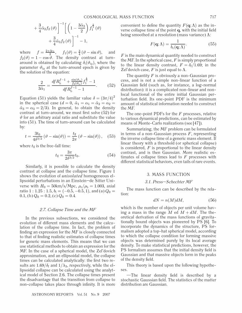
Similarly, it is possible to calculate the densitycontrast at collapse and the collapse time. Figure 1shows the evolution of unisolated homogeneous el-lipsoidal perturbations in an Einstein–de Sitter Uni-verse with H0 = 50km/s/Mpc, ρe/ρb = 1.003, axialratio 1 : 1.25 : 1.5, bi = (−0.5,−0.5, 1), and (a) Q0 =0.1, (b) Q0 = 0.2, (c) Q0 = 0.4.
2.7. Collapse Time and the MF
In the previous subsections, we considered theevolution of different mass elements and the calcu-lation of the collapse time. In fact, the problem offinding an expression for the MF is closely connectedto that of finding realistic estimates of collapse timesfor generic mass elements. This means that we canuse statistical methods to obtain an expression for theMF. In the case of a spherical model, the Zel’dovichapproximation, and an ellipsoidal model, the collapsetimes can be calculated analytically: the first two re-sults are 1.69/δl and 1/λ3, respectively, while the el-lipsoidal collapse can be calculated using the analyt-ical model of Section 2.6. The collapse times presentthe disadvantage that the transition from collapse tonon-collapse takes place through infinity. It is more
convenient to define the quantity F (q; Λ) as the in-verse collapse time of the point q, with the initial fieldbeing smoothed at a resolution (mass variance) Λ:
F (q; Λ) =1
bc(q; Λ). (55)
F is the main dynamical quantity needed to constructthe MF. In the spherical case, F is simply proportionalto the linear density contrast, F = δl/1.69; in theZel’dovich case, F is just equal to Λ.
The quantity F is obviously a non-Gaussian pro-cess, and is not a simple non-linear function of aGaussian field (such as, for instance, a log-normaldistribution): it is a complicated non-linear and non-local functional of the entire initial Gaussian per-turbation field. Its one-point PDF is the minimumamount of statistical information needed to constructthe MF.
The one-point PDFs for the F processes, relativeto various dynamical predictions, can be estimated bymeans of Monte-Carlo realizations (see [47]).
Summarizing, the MF problem can be formulatedin terms of a non-Gaussian process F , representingthe inverse collapse time of a generic mass element. Iflinear theory with a threshold (or spherical collapse)is considered, F is proportional to the linear densitycontrast, and is then Gaussian. More realistic es-timates of collapse times lead to F processes withdifferent statistical behaviors, even tails of rare events.
3. MASS FUNCTION
3.1. Press–Schechter MF
The mass function can be described by the rela-tion:
dN = n(M)dM, (56)
which is the number of objects per unit volume hav-ing a mass in the range M ed M + dM . The the-oretical derivation of the mass functions of gravita-tionally bound objects was pioneered by PS [6]. Toincorporate the dynamics of the structure, PS for-malism adopted a top-hat spherical model, accordingto which the collapse condition for forming massiveobjects was determined purely by its local averagedensity. To make statistical predictions, however, thePS formalism assumes that the initial density field isGaussian and that massive objects form in the peaksof the density field.
This theory is based upon the following hypothe-ses.
—The linear density field is described by astochastic Gaussian field. The statistics of the matterdistribution are Gaussian.
ASTRONOMY REPORTS Vol. 51 No. 9 2007
718 DEL POPOLO, YESILYURT
800
600
400
200
0
800
600
400
200
0
800
600
400
200
500 1000 1500 500 1000 1500
0 500 1000 1500
(‡) (b)
(c)
a
i
(
t
)/
a
i
(
t
0
)
a
i
(
t
)/
a
i
(
t
0
)
a
i
(
t
)/
a
i
(
t
0
)
R
b
R
b
R
b
Fig. 1. Evolution of unisolated homogeneous ellipsoidal perturbations in an Einstein–de Sitter Universe with H0 =50km/s/Mpc, ρe/ρb = 1.003, axial ratio 1 : 1.25 : 1.5, bi = (−0.5,−0.5, 1), and (a) Q0 = 0.1, (b) Q0 = 0.2, (c) Q0 = 0.4.Solid lines are numerical solutions (taken from [48]), dotted lines are analytical solutions.
—The evolution of density perturbations is de-scribed by the linear theory. Structures form in re-gions where the linearly evolved overdensity filteredwith a top-hat filter exceeds a threshold δc (δc = 1.68,obtained from the spherical collapse model [55]).
—When δ ≥ δc, regions collapse to points. Theprobability that an object forms at a certain point isproportional to the probability that the point is in aregion with δ ≥ δc, given by:
P (δ, δc) =
∞∫δc
dδ1
σ(2π)12
exp(− δ2
2σ2
). (57)
The mass function is given by:
ρ(M,z) = −ρ0∂P
∂MdM = n(M)MdM. (58)
If we add the conditions Ω = 1, |δk|2 ∝ kn, the PSsolution is autosimilar and has the form:
ρ(M,z) =ρ√2π
(n + 3
3
)(M
M∗z
)n+36
(59)
× exp[−1
2M
M∗(z)
n+33
]dM
M,
where M∗(z) ∝ (1 + z)−6
n+3 . There are several prob-lems with the theory, summarized below.
—Statistical problems: in the limit of vanishingsmoothing radii, or of infinite variance, the fraction ofcollapsed mass asymptotically approaches one-half.This is a signature of the linear theory: only initiallyoverdense regions, which constitute half of the mass,are able to collapse. Nevertheless, underdense regions
ASTRONOMY REPORTS Vol. 51 No. 9 2007
COSMOLOGICAL MASS FUNCTION 719
0.5
0.4
0.3
0.2
0.1
0–0.4 –0.2 0 0.2 0.4 0.6
M
, rel. units
MF
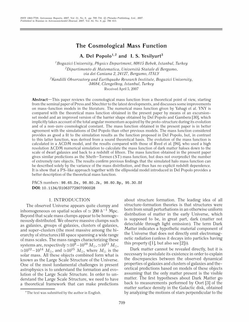
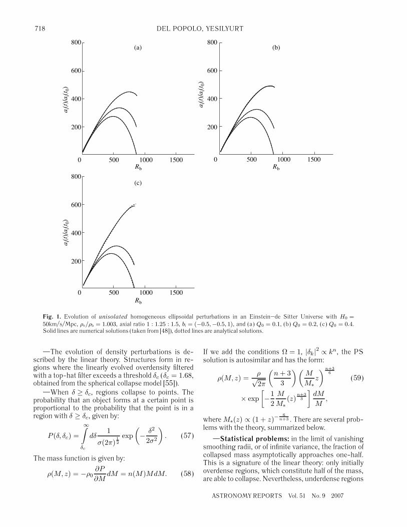
Fig. 2. Comparison of the PS mass function (solid curve)with the simulations of YNY (crosses with error bars).
can be included in larger overdense ones, or, moregenerally, non-collapsed regions have a finite proba-bility of being included in larger collapsed ones; this iscommonly called the cloud-in-cloud problem.
—Dynamical problems: the heuristic derivationof the PS MF bypasses all the complications relatedto the highly non-linear dynamics of gravitationalcollapse.
—Geometrical problems: to estimate the MFfrom the fraction of collapsed mass on a given scale, itis necessary to relate the mass of the formed structureto the resolution.
In practice, the true geometry of the collapsedregions in the Lagrangian space (i.e., as mapped inthe initial configuration) can be quite complex, espe-cially for intermediate and small masses; in this case,a different and more sophisticated mass assignmentmust be developed, so that the geometry is taken intoaccount. For instance, if structures are supposed toform at the peaks of the initial field, a different andmore geometrical way to count collapsed structurescould be based on peak abundances. In particular, thePS formula overestimates the abundance of haloesnear the characteristic mass M∗ and underestimatesthe abundance in the high-mass tail [YNY, 29, 43,66–68]. This discrepancy is not surprising, since thePS model, as any other analytical model, must makeseveral assumptions in order to obtain simple analyt-ical predictions.
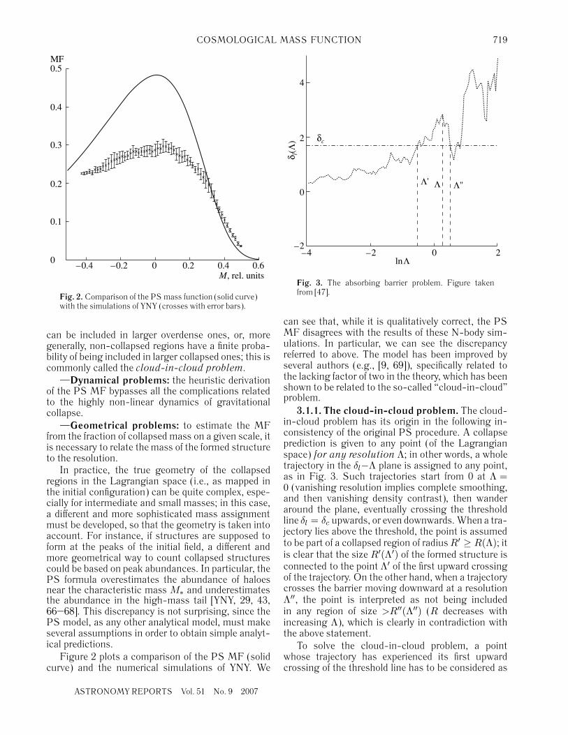
Figure 2 plots a comparison of the PS MF (solidcurve) and the numerical simulations of YNY. We
4
2
0
–2–4 –2 0 2
Λ
'
Λ Λ
''
δ
l
(
Λ
)
δ
c
ln
Λ
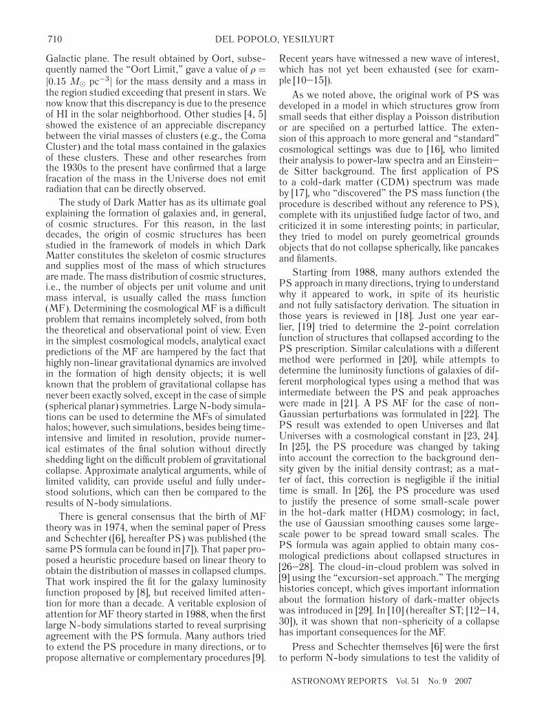
Fig. 3. The absorbing barrier problem. Figure takenfrom [47].
can see that, while it is qualitatively correct, the PSMF disagrees with the results of these N-body sim-ulations. In particular, we can see the discrepancyreferred to above. The model has been improved byseveral authors (e.g., [9, 69]), specifically related tothe lacking factor of two in the theory, which has beenshown to be related to the so-called “cloud-in-cloud”problem.
3.1.1. The cloud-in-cloud problem. The cloud-in-cloud problem has its origin in the following in-consistency of the original PS procedure. A collapseprediction is given to any point (of the Lagrangianspace) for any resolution Λ; in other words, a wholetrajectory in the δl−Λ plane is assigned to any point,as in Fig. 3. Such trajectories start from 0 at Λ =0 (vanishing resolution implies complete smoothing,and then vanishing density contrast), then wanderaround the plane, eventually crossing the thresholdline δl = δc upwards, or even downwards. When a tra-jectory lies above the threshold, the point is assumedto be part of a collapsed region of radius R′ ≥ R(Λ); itis clear that the size R′(Λ′) of the formed structure isconnected to the point Λ′ of the first upward crossingof the trajectory. On the other hand, when a trajectorycrosses the barrier moving downward at a resolutionΛ′′, the point is interpreted as not being includedin any region of size >R′′(Λ′′) (R decreases withincreasing Λ), which is clearly in contradiction withthe above statement.
To solve the cloud-in-cloud problem, a pointwhose trajectory has experienced its first upwardcrossing of the threshold line has to be considered as
ASTRONOMY REPORTS Vol. 51 No. 9 2007
720 DEL POPOLO, YESILYURT
collapsed at that scale, regardless of its subsequentdownward crossings. This can be done as follows:an absorbing barrier is placed in accordance withthe threshold line, so as to eliminate any downwardcrossing events [9]. Alternatively, a non-collapsecondition can be formulated as follows: a point is notcollapsed at Λ if its density contrast at any Λ′ < Λ isbelow the threshold [66].
The mathematical nature of the problem, and theresulting MF, depend strongly on the shape of thefilter. For general filters, trajectories are strongly cor-related in Λ, and then all the N-point correlations ofthe process at different resolutions must be known tosolve the problem. However, if the smoothing filtersharply cuts the density field in the Fourier space,then independent modes are added as the resolutionchanges, and the resulting trajectories are Gaussianrandom walks. This kind of filter is commonly called asharp k-space filter (SKS filter).
In the sharp k-space case, the problem is suitablysolved in the diffusion framework proposed by [9] (seenext subsection).
3.2. The Excursion-Set Approach
In this section, we review the formulation of theexcursion-set approach, mostly following [9]. Theterminology “excursion-set approach” was intro-duced in [9], to indicate that the MF determinationis based on the statistics of those regions where thelinear density contrast δl is larger than a thresholdδc (such regions are called excursion sets in thetheory of stochastic processes; see, e.g., [70]). The PSprocedure is clearly included in this approach. Thissection discusses works based on the excursion-setapproach.
3.2.1. Langevin equation. As previously de-scribed, the statistical properties of the Gaussian fieldδ(x) are completely specified by the two-point func-tion in Fourier space, which is related to the power-spectrum P (k) by 〈δ(k1)δ(k2)〉 = (2π)3δD(k1 +k2)P (k1), where δD represents the Dirac delta func-tion, and the brackets 〈·〉 denote ensemble aver-aging. Our Fourier transform convention is δ(k) =∫
dxδ(x)eik·x.We want now to study the statistical properties of
the density fluctuation field at some resolution scaleRf . This is introduced by convolving δ(x) with somefilter function W (|x′ − x|, Rf ),
δ(x, Rf ) =∫
dx′W (|x′ − x|, Rf )δ(x′) (60)
=1
(2π)3
∫dkW (kRf )δ(k)e−ik·x,
where W is the Fourier transform of the filter. At eachpoint x, the smoothed field represents the weightedaverage of δ(x) over a spherical region of charac-teristic dimension Rf centred in x. The detailedproperties of δ(x, Rf ) clearly depend on the specificchoice of the window function. The most com-monly used smoothing kernels are the top-hat filterWTH(|x|, Rf ) = 3Θ(Rf − |x|)/4πR3
f , where Θ(x) isthe Heaviside step function, and the Gaussian filterWG(x,Rf ) = (2πR2
f )−3/2 exp(−x2/2R2f ). Recently,
for convenience of analysis, top-hat filtering has alsobeen applied in momentum space, WSKS(k,Rf ) =Θ(kf − k), where kf = 1/Rf and kf = |kf |. Thiskernel is generally called a sharp k-space filter. Whileit is easy to associate a mass to real space top-hat filtering MTH(Rf ) = 4πρbR
3f/3, there is always
some arbitrariness in assigning a mass to the otherwindow functions. The most common procedure is tomultiply the average density by the volume enclosedby the filter, obtaining MG(Rf ) = (2π)3/2ρbR
3f and
MSKS(Rf ) = 6π2ρbk−3f [71]. An alternative proce-
dure, originally introduced by [72], corresponds tothe choice MSKS(Rf ) = 4πρbR
3TH/3, where RTH
is chosen by requiring σ2SKS(Rf ) = σ2
TH(RTH), andsimilarly for the Gaussian filter. In this way oneobtains good agreement with numerical simulationsof clustering growth [29].
In order to mimic the accretion of matter, a fullhierarchy of decreasing resolution scales Rf is con-sidered [9, 69, 71, 73]. The effect of varying Rf can beobtained by differentiating (60):
∂δ(x, Rf )∂Rf
=1
(2π)3(61)
×∫
dkδ(k)∂W (kRf )
∂Rfe−ik·x ≡ η(x, Rf ).
This has the form of a Langevin equation, whichshows how an infinitesimal change in the resolutionscale Rf affects the density-fluctuation field δ(x, Rf )in a given position x through the action of thestochastic force η(x, Rf ). In the limit Rf → ∞, wehave δ(x;Rf ) → 0, which can be adopted as an initialcondition for our first-order stochastic differentialequation. Thus, by solving this equation, we can as-sign to each point x a trajectory δ(x, Rf ) obtained byvarying the resolution scale Rf . Trajectories assignedto different neighboring points will be statisticallyinfluenced by the correlation properties of the forceη(x, Rf ), i.e., of the underlying Gaussian field δ(x).On the other hand, the coherence of each trajectoryalong Rf depends only on the analytical form ofthe filter function, and vanishes for a sharp k-space
ASTRONOMY REPORTS Vol. 51 No. 9 2007
COSMOLOGICAL MASS FUNCTION 721
window [9]. With such a filter, a new set of Fouriermodes of the unsmoothed distribution is added toδ(x, Rf ) by decreasing the smoothing length. Fora Gaussian field, this is completely independent ofthe previous increments, and each trajectory δ(x, Rf )becomes a Brownian random walk.
In the case of sharp k-space filtering, the no-tation greatly simplifies if we use the variance ofthe filtered density field, Λ ≡ σ2(kf ) = 〈δ(kf )2〉 =(2π2)−1
∫ kf
0 dkk2P (k), as the time variable. In thiscase, the stochastic process reduces to a Wienerprocess, namely,
∂δ(x,Λ)∂Λ
= ζ(x,Λ), (62)
with 〈ζ(x,Λ)〉 = 0 and
〈ζ(x,Λ1)ζ(x,Λ2)〉 = δD(Λ1 − Λ2). (63)
Below, we will adopt Λ as time variable, unless ex-plicitly stated otherwise. The solution of the Langevinequation (62) at an arbitrary point of space (the po-sition x is understood here) with the initial conditionδ(Λ = 0) = 0 is simply δ(Λ) =
∫ Λ0 dΛ′ζ(Λ′). Ensem-
ble averaging of this expression yields 〈δ(Λ)〉 = 0 and〈δ(Λ1)δ(Λ2)〉 = min(Λ1,Λ2), which uniquely deter-mine the Gaussian distribution of δ(Λ).
As was noted above, the PS model is intrinsicallyflawed by the cloud-in-cloud problem, i.e., the factthat a fluctuation on a given scale can contain sub-structures with smaller scales, such that the samefluid elements can be assigned according to the PScollapse criterion to haloes of different masses. More-over, in a hierarchical scenario, we expect to find allthe mass collapsed in objects of some scale, while thePS model can account for only half of this mass; thisproblem is intimately related to the fact that only halfthe volume is overdense in a Gaussian field. PS facedthe problem by simply multiplying their result by a“fudge factor” of two. In this section, we review howthe Langevin equations introduced above can be usedto extend the PS theory to make it possible to solveboth problems.
The solution of the cloud-in-cloud problem wasgiven by [9, 69, 73]. They considered at any givenpoint the trajectory δ(Rf ) as a function of the filteringradius, and then determined the largest Rf for whichδ(Rf ) crosses the threshold tf (zf ) corresponding tothe formation redshift zf moving upward. This de-termines the largest mass that has collapsed at thatpoint, with all sub-structures having been erased.Thus, the computing the mass function is equivalentto calculating the fraction of trajectories that firstcross the threshold tf moving upward as the scale Mdecreases. The solution of the problem is enormously
simplified for Brownian trajectories, i.e., for sharp k-space filtered density fields. In this case, it is onlynecessary to solve the Fokker–Planck equation forthe probability density W(δ,Λ)dδ corresponding tothe probability that the stochastic process at Λ adoptsa value in the interval δ, δ + dδ,
∂W(δ,Λ)∂Λ
=12
∂2W(δ,Λ)∂δ2
, (64)
with the absorbing boundary condition W(tf ,Λ) = 0and the initial condition W(δ, 0) = δD(δ). The solu-tion is well known [74]:
W(δ,Λ, tf )dδ =1√2πΛ
(65)
×[exp
(− δ2
2Λ
)− exp
(−(δ − 2tf )2
2Λ
)]dδ.
Defining S(Λ, tf ) =∫ tf−∞ dδW(δ,Λ, tf ) as the sur-
vival probability of the trajectories, we can obtain thedensity probability distribution of the first-crossingvariances via differentiation:
P1(Λ) = −∂S(Λ, tf )∂Λ
= − ∂
∂Λ(66)
×tf∫
−∞
dδW(δ,Λ, tf ) =[−1
2∂W(δ,Λ, tf )
∂δ
]tf
−∞
=tf√2πΛ3
exp
(−
t2f2Λ
).
The function P1(Λ)dΛ yields the probability that a re-alization of the random walk is absorbed by the barrierin the interval (Λ,Λ + dΛ), or, by the ergodic theo-rem, the probability that a fluid element belongs to astructure with mass in the range [M(Λ + dΛ),M(Λ)].Finally, the comoving number density of haloes withmasses in the interval [M,M + dM ] that have col-lapsed at redshift zf is
n(M,zf )dM =ρb
MP1(Λ)
∣∣∣∣ dΛdM
∣∣∣∣ dM. (67)
Inserting P1(Λ) from (66) into this last equationyields the well-known PS for the mass function:
n(M,zf )dM =ρbtf (zf )√
2π1
M2√
Λ(M)(68)
×∣∣∣∣ d ln Λd ln M
∣∣∣∣ exp(− tf (zf )2
2Λ(M)
)dM.
The original fudge factor of two of the PS approach isnow naturally justified.
Previous investigations (e.g., [9, 69]) have shownthat only for sharp k-space filtering it is possible
ASTRONOMY REPORTS Vol. 51 No. 9 2007
722 DEL POPOLO, YESILYURT
to write an analytical formula for the mass functionobtained from the excursion-set approach. Numericalsolutions of the cloud-in-cloud problem with phys-ically more acceptable smoothing kernels, such asGaussians and top-hats, result in mass functions thatare a factor of two lower in the high-mass tail andhave different small-mass slopes than the PS for-mula. The standard interpretation of this result is thatthe excursion-set method is not reliable for M � M∗,where M∗, defined by Λ(M∗) = t2f , is the typical masscollapsing at zf .
3.2.2. Merging histories. Merging histories arean important piece of information in the formationhistory of dark-matter objects. They are a naturaloutcome of MF theories: a point mass found in anobject of mass M at a given time will be found in an-other, more massive, object at a subsequent time; theconditional probabilities associated with such eventscan be used to construct the statistics of the accretionand merging histories of collapsed structures. Thiswas first attempted by Carlberg and Couchman [35],whose results are in contradiction with more recentworks outlined below. Merging histories were con-structed using the PS formalism in [75], obtainingthe same results as were obtained using the diffusionformalism reported below.
Suppose that we have smoothed the initial den-sity distribution on a scale R using some sphericallysymmetric window function WM (r), where M(R) isthe average mass contained within the window func-tion. There are various possible choices for the formof the window function (c.f. [71]). We use a real-space, top-hat window function, WM (r) = Θ(R −r)(4πR3/3)−1, where Θ is the Heaviside step func-tion. In this case, M = 4πρ0R
3/3, where ρ0 is themean mass density of the Universe. The mass vari-ance S(M) ≡ σ2(M) can be calculated from
σ2(M) =1
2π2
∫P (k)W 2(kR)k2dk, (69)
where P (k) is the power spectrum of the matter den-sity fluctuation, and W (kR) is the Fourier transformof the real-space top hat.
The “excursion-set” derivation due to [9] leadsnaturally to the extended PS formalism. Thesmoothed field δ(M) is a Gaussian random variablewith zero mean and variance S. The value of δexecutes a random walk as the smoothing scaleis changed. Adopting an ansatz similar to that ofthe original PS model, we associate the fractionof matter in collapsed objects in the mass intervalM,M + dM at time t with the fraction of trajectoriesthat make their first upward crossing through thethreshold ω ≡ δc(t) in the interval S, S + dS. Thiscan be translated to a mass interval via (69). The
threshold δc(t) corresponds to the critical densityat which a pertubation will separate from the back-ground expansion, turn around, and collapse. It isextrapolated using linear theory, δc(t) = δc,0/Dlin(z),where Dlin(z) is the linear growth function. The halo-mass function (here, in the notation of [71]) is then:
f(S, ω)dS =1√2π
ω
S3/2exp
[−ω2
2S
]dS. (70)
The conditional mass function, the fraction of thetrajectories in halos with mass M1 at z1 that are inhalos with mass M0 at z0 (M1 < M0, z0 < z1), is
f(S1, ω1|S0, ω0)dS1 =1√2π
(ω1 − ω0)(S1 − S0)3/2
(71)
× exp[− (ω1 − ω0)2
2(S1 − S0)
]dS1.
The probability that a halo of mass M0 at redshift z0
had a progenitor in the mass range (M1,M1 + dM1)is given by [71]:
dP
dM1(M1, z1|M0, z0)dM1 (72)
=M0
M1f(S1, ω1|S0, ω0)
∣∣∣∣ dS
dM
∣∣∣∣ dM1,
where the factor M0/M1 converts the counting frommass weighting to number weighting.
We can now derive two more useful quantities.Given the mass of a parent halo M0 and the redshiftstep z0 → z1, the average number of progenitors withmasses larger than Ml is:
N ≡ 〈Np(M |M0)〉 (73)
=
M0∫Ml
dMM0
M
dP
dM(M,z1|M0, z0).
We can also readily calculate the average fraction ofM0 that was in the form of progenitor halos of massM > Ml:
fp =
∞∫Ml
dMdP
dM(M,z1|M0, z0), (74)
and define the complimentary quantity for the aver-age fraction of M0 that came from “accreted” mass,facc = 1 − fp.
In order to describe the accretion history of anobject, it suffices to lower the barrier in a continuousway and follow the position in Λ of the first up-ward crossing point: if this displays a discontinuousjump (as happens when the trajectory goes down andthen up again), the object containing the mass point
ASTRONOMY REPORTS Vol. 51 No. 9 2007
COSMOLOGICAL MASS FUNCTION 723
considered suffers a discontinuous merging with astructure of comparable size; if the point moves con-tinuously, the object is just accreting material. It isclear that, if the trajectory is a random walk, the firstupward crossing point will always perform discretejumps; continuous accretion will be recognized onlyif an (arbitrary) minimum resolution step is fixed.
A Monte Carlo approach to simulate ensembles offormation histories based on realizing a large num-ber of random walks was also proposed in [71]. ThisMonte Carlo method for simulating merging historiesis commonly used to model the formation of viri-alized galactic halos, with the gas dynamics beinginserted “by hand.” As a matter of fact, Peacock andHeavens [69] found a weak inconsistency in theirformalism (a probability density that went slightlynegative), probably due to their simplicistic mass as-signment. These same authors compared their resultswith N-body simulations, finding an overall satisfac-tory agreement [29].
Finally, a complete analytical description for themerging histories of objects formed from a Poissondistribution of seed masses was obtained in [76, 77]—the problem analyzed by the original PS paper.
3.3. Peak Approach
An idea that can be traced back to [78] is the pos-siblity that structures form at the peaks of the initialdensity field. This idea became a standard paradigmin biased galaxy scenarios: it was noted in [79] thathigh-level peaks show an enhanced correlation withrespect to the underlying matter field, providing anexplanation for the large correlation length of clusterswith respect to galaxies, and giving freedom to tunethe normalization of the CDM model to reproduce thelarge-scale distribution of galaxies. A number of sta-tistical expectation values for the peaks of a Gaussianrandom field were calculated in [72, 80], as the num-ber density of peaks of a given height. This quantityseemed suitable for the determination of a peak MF,but two important problems, recognized by [72] (whodid not attempt to determine the MF from the peaknumber density) hampered this process: (i) it was notclear which mass had to be assigned to a peak; (ii) thepeak number density was based on the initial fieldsmoothed at a single scale, so the peak MF sufferedfrom the same cloud-in-cloud problem (the peak-in-peak problem) as the PS approach.
The excursion-set and peak approaches are some-what complementary. In fact, excursion sets are ef-fective in determining the total fraction of collapsedmass, and then the global normalization, but are notaccurate in deciding how the collapsed mass frag-ments into clumps, i.e., in counting the number ofobjects formed. On the contrary, the peak approach
clearly determines the number of formed objects, butdoes not determine the mass to be associated with thestructures, and hence the global normalization.
A peak MF can be formulated as follows. Let usdenote npk(δl; Λ) to be the number density of peakswith linear density contrast δl (per unit δl interval); theinitial field is assumed to be smoothed at a resolutionΛ. Then, if Mpk(δl,Λ) is the mass associated to thepeak, and if the variable M is used in place of Λ (theuncertainty in the Λ ←→ M relation can be absorbedin the Mpk definition), the fraction of collapsed masscan be written:
Ω(>M) =1ρ
∞∫δc
dδlnpk(δl,M)Mpk(δl,M), (75)
where δc is a density threshold for the peak. Using thesame “golden rule” as in the PS approach yields:
n(M)dM =∣∣∣∣d[npk(δc;M)Mpk(δc,M)]
dM
∣∣∣∣ dM. (76)
As a matter of fact, there is no general agreementon the actual validity of the peak paradigm. From thetheoretical point of view, structures are not predictedto form at the peaks of the initial field; for instance,in the Zel’dovich approximation, structures form atthe peaks of the largest eigenvalue of the deformationtensor. The peak paradigm cannot then be valid ingeneral, except for the highest peaks. Some numer-ical simulations [81, 82] have shown that galaxy-sizepeaks are often disrupted or merge with larger struc-tures as a result of tidal interactions with externalstructures. Manrique and Salvador-Sole [83] arguedthat such results are due to the lack of correction forthe peak-in-peak problem. On the other hand, thepeak-patch structures used by Bond and Myers [84]to correct the peak-in-peak problem represent N-body structures well.
The first to use the peak MF, with Mpk given bythe mass inside the filter (and independent of δc), wereNarayan and White [33], who found good agareementwith their N-body simulations; however, the peak MFis not much different from the PS peak in the rangetested by those simulations. In addition, Bond [85]proposed an analogous formula to model the MF ina biased CDM scenario.
Alternative, more motivated expressions for themasses of peaks were proposed by a number of au-thors. The peak was modeled as a triaxial ellipsoidin [80], and its mass estimated using the volume ofthe ellipsoid within δl > 0. Following a suggestion in[72], the mass of the peak was also determined asthe mass contained within the radius where the meandensity profile is equal to its dispersion in [86]. Thepeak was also modeled as an ellipsoid in [87], and its
ASTRONOMY REPORTS Vol. 51 No. 9 2007
724 DEL POPOLO, YESILYURT
mass estimated using the volume inside the ellipsoidsurface with a density larger that a given threshold.Finally, in [69], the mass of a (Gaussian-smoothed)peak was estimated as the mass contained in a sphereproducing the same variance as that obtained by top-hat smoothing; it was also noted that the peak massought to satsify the constraint of a global normaliza-tion of the MF.
All these reasonable definitions give rise to dif-ferent MFs. To decide which mass assignment iscorrect, two things are required: (i) the peak-in-peakproblem must be solved, and then (ii) the mass as-signments must be compared to N-body simulations.Attempts in this direction are described in the nextsubsection.
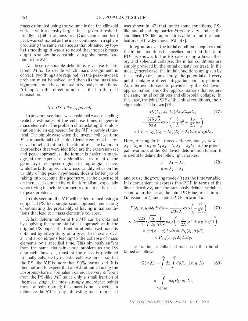
3.4. PS-Like Approach
In previous sections, we considered ways of findingrealistic estimates of the collapse times of genericmass elements. The problem of translating this infor-mation into an expression for the MF is purely statis-tical. The simple case when the inverse collapse timeF is proportional to the initial density contrast has re-ceived much attention in the literature. The two mainapproaches that were identified are the excursion-setand peak approaches: the former is easier to man-age, at the expense of a simplified treatment of thegeometry of collapsed regions in Lagrangian space,while the latter approach, whose validity relies on thevalidity of the peak hypothesis, does a better job oftaking into account this geometry, at the expense ofan increased complexity of the formalism, especiallywhen trying to include a proper treatment of the peak-in-peak problem.
In this section, the MF will be determined using asimplified PS-like, single-scale approach, consistingof estimating the probability of having initial condi-tions that lead to a mass element’s collapse.
A first determination of the MF can be obtainedby applying the same statistical approach as in theoriginal PS paper: the fraction of collapsed mass isobtained by integrating, on a given fixed scale, overall initial conditions leading to the collapse of masselements by a specified time. This obviously suffersfrom the same cloud-in-cloud problem as the PSapproach; however, most of the mass is predictedto finally collapse by realistic collapse times, so thatthe PS-like MF is more than 90% normalized. It isthen natural to expect that an MF obtained using theabsorbing-barrier formalism cannot be very differentfrom the PS-like MF, since only a small fraction ofthe mass lying at the most strongly underdense pointsmust be redistributed; this mass is not expected toinfluence the MF in any interesting mass ranges. It
was shown in [47] that, under some conditions, PS-like and absorbing-barrier MFs are very similar; thesimplified PS-like approach is able to find the mainfeatures of the dynamical MF [47].
Integration over the initial conditions requires thatthe initial conditions be specified, and that their jointPDF is known. In the PS case, using a linear the-ory and spherical collapse, the initial conditions aresimply provided by the initial density contrast. In themost general case, the initial conditions are given bythe density (or, equivalently, the potential) at everypoint, making a direct integration hard to perform.An intermediate case is provided by the Zel’dovichapproximation, and other approximations that requirethe same initial conditions and ellipsoidal collapse. Inthis case, the joint PDF of the initial conditions, the λeigenvalues, is known [78]:
Pλ(λ1, λ2, λ3)dλ1dλ2dλ3 (77)
=675
√5
8πΛ3exp
(− 3
Λμ2
1 +152Λ
μ2
)
× (λ1 − λ2)(λ1 − λ3)(λ2 − λ3)dλ1dλ2dλ3.
Here, Λ is again the mass variance, and μ1 = λ1 +λ2 + λ3 and μ2 = λ1λ2 + λ1λ3 + λ2λ3 are the princi-pal invariants of the Zel’dovich deformation tensor. Itis useful to define the following variables:
x = λ1 − λ2, (78)
y = λ2 − λ3,
and to use the growing mode b(t) as the time variable.It is convenient to express this PDF in terms of thelinear density δl and the previously defined variablesx and y. in this case, the joint PDF factorizes into aGaussian for δl and a joint PDF for x and y:
P (δl, x, y)dδldxdy =1√2πΛ
exp(− δ2
l
2Λ
)(79)
× dδl2254
√52π
1Λ5/2
exp(− 5
2Λ(x2 + xy + y2)
)
× xy(x + y)dxdy = Pδl(δl,Λ)dδl
× Px,y(x, y,Λ)dxdy.
The fraction of collapsed mass can then be ob-tained as follows:
Ω(<Λ) =
∞∫0
dx
∞∫0
dyPx,y(x, y,Λ) (80)
×∞∫
δc(x,y)
dδlPδl(δl,Λ),
ASTRONOMY REPORTS Vol. 51 No. 9 2007
COSMOLOGICAL MASS FUNCTION 725
where the function δc(x, y), which replaces the PS δc
parameter, is defined as the solution of the equation:
bc(δc, x, y) = b(t0), (81)
where b(t0) is the time for which the MF is desired(usually equal to one). By writing the function δc asδ0 − f(x, y), where δ0 is the spherical value 1.69 andthe positive function f(x, y), vanishing at the origin,gives the effect of the shear, it is possible to write then(Λ) function as:
n(Λ) = nPS(Λ) × I(Λ), (82)
where nPS(Λ) is the PS curve, and I(Λ) is a correc-tion term:
I(Λ) =1Λ
∞∫0
dx
∞∫0
dyPx,y(x, y) (83)
× exp(− 1
2Λf(x, y)2 +
δ0
Λf(x, y)
)
×(
1 − 1δ0
(f − x
∂f
∂x− y
∂f
∂y
)).
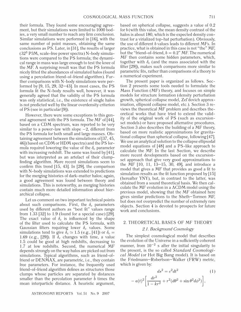
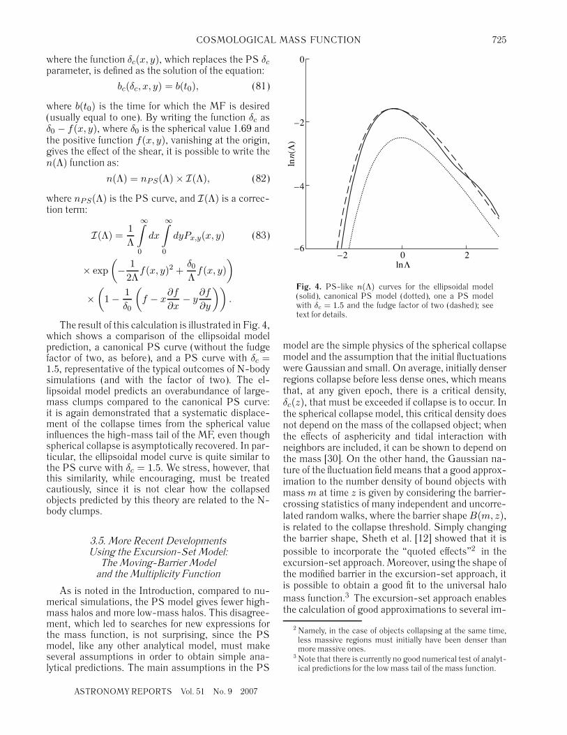
The result of this calculation is illustrated in Fig. 4,which shows a comparison of the ellipsoidal modelprediction, a canonical PS curve (without the fudgefactor of two, as before), and a PS curve with δc =1.5, representative of the typical outcomes of N-bodysimulations (and with the factor of two). The el-lipsoidal model predicts an overabundance of large-mass clumps compared to the canonical PS curve:it is again demonstrated that a systematic displace-ment of the collapse times from the spherical valueinfluences the high-mass tail of the MF, even thoughspherical collapse is asymptotically recovered. In par-ticular, the ellipsoidal model curve is quite similar tothe PS curve with δc = 1.5. We stress, however, thatthis similarity, while encouraging, must be treatedcautiously, since it is not clear how the collapsedobjects predicted by this theory are related to the N-body clumps.
3.5. More Recent DevelopmentsUsing the Excursion-Set Model:
The Moving-Barrier Modeland the Multiplicity Function
As is noted in the Introduction, compared to nu-merical simulations, the PS model gives fewer high-mass halos and more low-mass halos. This disagree-ment, which led to searches for new expressions forthe mass function, is not surprising, since the PSmodel, like any other analytical model, must makeseveral assumptions in order to obtain simple ana-lytical predictions. The main assumptions in the PS
–2 0 2ln
Λ
–6
–2
–4
0
ln
n
(
Λ
)Fig. 4. PS-like n(Λ) curves for the ellipsoidal model(solid), canonical PS model (dotted), one a PS modelwith δc = 1.5 and the fudge factor of two (dashed); seetext for details.
model are the simple physics of the spherical collapsemodel and the assumption that the initial fluctuationswere Gaussian and small. On average, initially denserregions collapse before less dense ones, which meansthat, at any given epoch, there is a critical density,δc(z), that must be exceeded if collapse is to occur. Inthe spherical collapse model, this critical density doesnot depend on the mass of the collapsed object; whenthe effects of asphericity and tidal interaction withneighbors are included, it can be shown to depend onthe mass [30]. On the other hand, the Gaussian na-ture of the fluctuation field means that a good approx-imation to the number density of bound objects withmass m at time z is given by considering the barrier-crossing statistics of many independent and uncorre-lated random walks, where the barrier shape B(m, z),is related to the collapse threshold. Simply changingthe barrier shape, Sheth et al. [12] showed that it ispossible to incorporate the “quoted effects”2 in theexcursion-set approach. Moreover, using the shape ofthe modified barrier in the excursion-set approach, itis possible to obtain a good fit to the universal halomass function.3 The excursion-set approach enablesthe calculation of good approximations to several im-
2 Namely, in the case of objects collapsing at the same time,less massive regions must initially have been denser thanmore massive ones.
3 Note that there is currently no good numerical test of analyt-ical predictions for the low mass tail of the mass function.
ASTRONOMY REPORTS Vol. 51 No. 9 2007
726 DEL POPOLO, YESILYURT
portant quantities, such as the “unconditional” and“conditional” mass functions. Formulas for calculat-ing these quantities starting from the shape of thebarrier are given in [12].
Below, we will use an improved version of thebarrier obtained in [30] to obtain the MFs, which shallbe compared with the MFs obtained by PS, ST [10](hereafter J01), YNY, and also with the numericalsimulations of YNY [15].
In order to calculate the barrier shape, we willfollow the model of [30]. The equation governing thecollapse of a density perturbation taking into accountthe acquisition of angular momentum by protostruc-tures can be obtained using the model of [88] (seealso [30, 49]).
Let’s consider an ensemble of gravitationallygrowing mass concentrations and suppose that thematerial in each system collects within the samepotential well, with an inward pointing acceler-ation given by g(r) (see [30]). We denote dP =f(L, rvr, t)dLdvrdr to be the probability that a parti-cle can be found in the range of proper radius from rto r + dr, in the range of radial velocity from vr = r tovr + dvr and with angular momentum L = rvθ in therange dL. The radial acceleration of the particle is:
dvr
dt=
L2(r)M2r3
− g(r) =L2(r)M2r3
− GM
r2. (84)
Equation (84) can be derived from a potential. Fur-ther, it follows from Liouville’s theorem that the dis-tribution function, f , satisfies the collisionless Boltz-mann equation:
∂f
∂t+ vr
∂f
∂r+
∂f
∂vr
[L2
r3− g(r)
]= 0. (85)
Assuming a non-zero cosmological constant, (84)becomes:
dvr
dt= −GM
r2+
L2(r)M2r3
+Λ3
r (86)
[24, 30, 49, 88]. Integrating (86) yields:
12
(dr
dt
)2
=GM
r+∫
L2
M2r3dr +
Λ6
r2 + ε, (87)
where the value of the specific binding energy of theshell, ε, can be obtained using the condition for turn-around, dr
dt = 0.
In turn, the binding energy of a growing mode so-lution is uniquely given by the linear overdensity, δi, attime ti. Using this overdensity in the linear theory, wecan find the result for the turn-around epoch and thenthe collapse. We find the binding energy of the shell,C, using the relation between v and δi for the growing
mode [53] in (87), and finally the linear overdensity atthe time of collapse is given by:
δc = δco
⎡⎣1 +
rta∫ri
rtaL2dr
GM3r3+ Λ
rtar2
6GM
⎤⎦ (88)
� δco
[1 +
β1
να1+
ΩΛβ2
να2
],
where α1 = 0.585, β1 = 0.46, α2 = 0.4, and β2 =0.02, δco = 1.68 is the critical threshold for a sphericalmodel, ri is the initial radius, rta is the turn-aroundradius, and L is the angular momentum. The angularmomentum appearing in (88) is the total angularmomentum acquired by the proto-structure during itsevolution. We can calculate L using the same modelas is described in [30, 49] (more information aboutthe model and some of the model limits can be foundin [89]).
The CDM spectrum used to calculate the massfunction is that of [72] (Eq. (G3)), with the transferfunction:
T (k) =[ln (1 + 2.34q)]
2.34q[1 + 3.89q (89)
+ (16.1q)2 + (5.46q)3 + (6.71)4]−1/4
(where q = kθ1/2
ΩXh2 Mpc−1 . Here, θ = ρer/(1.68ργ) rep-
resents the ratio of the energy densities in relativisticparticles and in photons (θ = 1 corresponds to pho-tons and the three flavors of relativistic neutrinos).The power spectrum was normalized to reproducethe observed abundance of rich clusters of galaxies(e.g., [90]).
In the excursion-set approach, the average co-moving number density of haloes of mass m, theuniversal or “unconditional” mass function, n(m, z),is given by [9]:
n(m, z) =ρ
m2
d log ν
d log mνf(ν), (90)
where ρ is the background density, ν =(
δc(z)σ(m)
)2is
the ratio of the critical overdensity required for col-lapse in the spherical model, δc(z), and the rms den-sity fluctuation σ(m), on the scale r of the initial sizeof the object m. The function νf(ν) is obtained bycomputing the distribution of first crossings, f(ν)dν,of a barrier B(ν) by independent, uncorrelated Brow-nian motion random walks. The mass function canthen be calculated once a shape for the barrier is givenand the power spectrum is known. In the case ofspherical collapse, characterized by a constant barrier(for all ν), PS and [9] obtained:
νf(ν) =( ν
2π
) 12 exp(−ν
2). (91)
ASTRONOMY REPORTS Vol. 51 No. 9 2007
COSMOLOGICAL MASS FUNCTION 727
In the case of a nonspherical collapse, the shape ofthe barrier is no longer a constant, and moreoverdepends on mass [12, 30]. As was shown by PS, for a
given barrier shape, B(S), where S ≡ S∗(
σσ∗
)2= S∗
ν
and σ∗ =√
S∗ = δco, the first crossing distribution isapproximated well by:
f(S)dS = |T (S)| exp(−B(S)2
2S)dS/S√
2πS, (92)
where T (S) is the sum of the first few terms in theTaylor expansion of B(S):
T (S) =5∑
n=0
(−S)n
n!∂nB(S)
∂Sn. (93)
The quantity Sf(S, t) is a function of the variableν alone, where ν ≡ (δc(t)/σ(M))2. Since δc andσ evolve with time in the same way, the quantitySf(S, t) is independent of time. Setting 2Sf(S, t) =νf(ν), we obtain the MF f(ν); this is why the shapeof the barrier influences the form of the MF.
In the case of the ellipsoidal barrier shape given inST:
B(σ2, z) =√
aδc(z)[1 +
β
(aν)α
](94)
Eqs. (92), (93), give, after truncating the expansion atn = 5 (see ST):
νf(ν) =√
aν/2π[1 + β(aν2)−αg(α)] (95)
× exp(−0.5aν2[1 + β(aν2)−α]2
),
where
g(α) (96)
=∣∣∣∣1 − α +
α(α − 1)2!
− . . . − α(α − 1) . . . (α − 4)5!
∣∣∣∣.Using the values for β and α of [13] (a = 0.707,
δc(z) = 1.686(1 + z), β � 0.485 and α � 0.615) in(95) yields (PS):
νf(ν) � A1
(1 +
0.094(aν)0.6
)√aν
2π(97)
× exp
{−aν
[1 +
0.5(aν)0.6
]2/2
}
with A1 � 1. This last result is in good agreementwith the fit of the simulated first crossing distribu-tion (ST):
νf(ν)dν = A2
(1 +
1(aν)p
)√aν
2πexp(−aν/2)
(98)
where p = 0.3, and a = 0.707. The normalization fac-tor A2 must satisfy the constraint:
∞∫0
f(ν)dν = 1 (99)
and as a consequence it is not an independent param-eter, but is expressed in the form:
A2 =[1 + 2−pπ−1/2Γ(1/2 − p)
]−1= 0.3222.
(100)
If the barrier takes into account the cosmologicalconstant, as in (88), we find using the same methodthat lead to (95):
νf(ν) = A1
(1 +
β1g(α1)(aν)α1
+β2g(α2)(aν)α2
)√aν
2π(101)
× exp
{−aν
[1 +
β1
(aν)α1+
β2
(aν)α2
]2/2
}.
In the case of the barrier given in (88) with Λ = 0,the “unconditional” MF can be approximated:
νf(ν) � A4
(1 +
b
(aν)0.585
)√aν
2π(102)
× exp
{−acν
[1 +
d
(aν)0.585
]2}
,
where a = 0.707, b = 0.1218, c = 0.4019, d = 0.5526and A4 � 1.75 is obtained from the normalizationcondition. In the case of the barrier (88) with non-zero cosmological constant, a good approximation tothe MF is given by:
νf(ν) � A5
(1 +
0.1218(aν)0.585 +
0.0079(aν)0.4
)√aν
2π(103)
× exp
{−0.4019aν
[1 +
0.5526(aν)0.585 +
0.02(aν)0.4
]2}
where A5 = 1.75. As we indicated above, for com-pleteness, we add to the previous functions—PS, ST,and (103)—the MF of J01, which satisfies the equa-tion:
νf(ν) = 0.315 exp(−|0.61 + ln[σ−1(M)]|3.8) =(104)
0.315 exp(−|0.61 + ln√
ν − ln δc|3.8).
The above formula is valid for −1.2 < ln√
ν − ln δc <1.05.
In their Eq. (7), YNY proposed the following func-tion to fit the numerical MF:
νf(ν) = A6[1 + (B√
ν)/√
2)C ]√
νD (105)
ASTRONOMY REPORTS Vol. 51 No. 9 2007
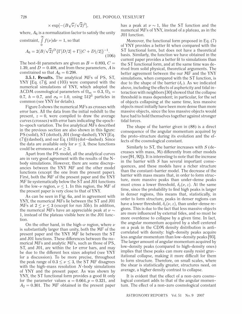
728 DEL POPOLO, YESILYURT
× exp[−(B√
ν/√
2)2],
where, A6 is a normalization factor to satisfy the unity
constraint,∞∫0
f(ν)dν = 1, so that
A6 = 2(B/√
2)D{Γ[D/2] + Γ[(C + D)/2]}−1.(106)
The best-fit parameters are given as B = 0.893, C =1.39, and D = 0.408, and from these parameters, A isconstrained so that A6 = 0.298.
3.5.1. Results. The analytical MFs of PS, ST,YNY [Eq. (7)], and (103) were compared with thenumerical simulations of YNY, which adopted theΛCDM cosmological parameters of Ωm = 0.3, Ωλ =0.7, h = 0.7, and σ8 = 1.0, using 5123 particles incommon (see YNY for details).
Figure 5 shows the numerical MFs as crosses witherror bars. All the data from the initial redshift to thepresent, z = 0, were compiled to draw the averagecurves (crosses) with error bars indicating the epoch-to-epoch variation. The five analytical MFs describedin the previous section are also shown in this figure:PS (solid), ST (dotted), J01 (long-dashed), YNY [Eq.(7)] (dashed), and our Eq. (103) (dot–dashed). Sincethe data are available only for ν ≤ 3, these functionscould be erroneous at ν ≥ 3.
Apart from the PS model, all the analytical curvesare in very good agreement with the results of the N-body simulations. However, there are some discrep-ancies between the YNY MF and the other modelfunctions (except the one from the present paper).First, both the MF of the present paper and the YNYMF lie systematically below the ST and J01 functionsin the low-ν region, ν ≤ 1. In this region, the MF ofthe present paper is very close to that of YNY.
As can be seen in Fig. 6a, and in agreement withYNY, the numerical MFs lie between the ST and J01MFs at 2 ≤ ν ≤ 3 (except for run 35b). In addition,the numerical MFs have an appreciable peak at ν ∼1, instead of the plateau visible here in the J01 func-tion.
On the other hand, in the high-ν region, where νis substantially larger than unity, both the MF of thepresent paper and the YNY MF lie between the STand J01 functions. These differences between the nu-merical MFs and analytic MFs, such as those of PS,ST, and J01, are within the 1σ error bars, and maybe due to the different box sizes adopted (see YNYfor a discussion). To be more precise, throughoutthe peak range of 0.3 ≤ ν ≤ 3, the ST MF disagreeswith the high-mass resolution N-body simulationsof YNY and the present paper. As was shown byYNY, the ST functional form provides a good fit onlyfor the parameter values a = 0.664, p = 0.321, andA2 = 0.301. The MF obtained in the present paper
has a peak at ν ∼ 1, like the ST function and thenumerical MFs of YNY, instead of a plateau, as in theJ01 function.
Moreover, the functional form proposed in Eq. (7)of YNY provides a better fit when compared with theST functional form, but does not have a theoreticalbasis. Similarly, the function we have obtained in thecurrent paper provides a better fit to simulations thanthe ST functional form, and at the same time was de-rived from solid physical, theoretical arguments. Thebetter agreement between the our MF and the YNYsimulations, when compared with the ST function, isdue to the shape of the barrier (δc). As we indicatedabove, including the effects of asphericity and tidal in-teraction with neighbors [30] showed that the collapsethreshold is mass dependent; in particular, for the setof objects collapsing at the same time, less massiveobjects must initially have been more dense than moremassive objects, since the less massive objects wouldhave had to hold themselves together against strongertidal forces.
The shape of the barrier given in (88) is a directconsequence of the angular momentum acquired bythe proto-structure during its evolution and the ef-fects of the cosmological constant.
Similarly to ST, the barrier increases with S (de-creases with mass, M) differently from other models(see [91, 92]). It is interesting to note that the increasein the barrier with S has several important conse-quences, and these models have a richer structurethan the constant-barrier model. The decrease of thebarrier with mass means that, in order to form struc-ture, more massive peaks than under-dense peaksmust cross a lower threshold, δc(ν, z). At the sametime, since the probability to find high peaks is largerin denser regions, this means that, statistically, inorder to form structure, peaks in denser regions canhave a lower threshold, δc(ν, z), than under-dense re-gions. This is due to the fact that less massive objectsare more influenced by external tides, and so must bemore overdense to collapse by a given time. In fact,the angular momentum acquired by a shell centeredon a peak in the CDM density distribution is anti-correlated with density: high-density peaks acquireless angular momentum than low-density peaks [93].The larger amount of angular momentum acquired bylow-density peaks (compared to high-density ones)implies that these peaks can more easily resist grav-itational collapse, making it more difficult for themto form structure. Therefore, on small scales, wherethe shear is statistically greater, structures need, onaverage, a higher density contrast to collapse.
It is evident that the effect of a non-zero cosmo-logical constant adds to that of the angular momen-tum. The effect of a non-zero cosmological constant
ASTRONOMY REPORTS Vol. 51 No. 9 2007
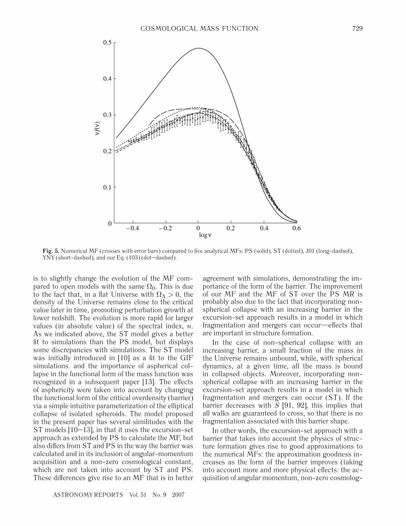
COSMOLOGICAL MASS FUNCTION 729
0.5
0.4
0.3
0.2
0.1
0– 0.4 – 0.2 0 0.2 0.4 0.6
log
ν
ν
f
(
ν
)
Fig. 5. Numerical MF (crosses with error bars) compared to five analytical MFs: PS (solid), ST (dotted), J01 (long-dashed),YNY (short-dashed), and our Eq. (103) (dot–dashed).
is to slightly change the evolution of the MF com-pared to open models with the same Ω0. This is dueto the fact that, in a flat Universe with ΩΛ > 0, thedensity of the Universe remains close to the criticalvalue later in time, promoting perturbation growth atlower redshift. The evolution is more rapid for largervalues (in absolute value) of the spectral index, n.As we indicated above, the ST model gives a betterfit to simulations than the PS model, but displayssome discrepancies with simulations. The ST modelwas initially introduced in [10] as a fit to the GIFsimulations. and the importance of aspherical col-lapse in the functional form of the mass function wasrecognized in a subsequent paper [13]. The effectsof asphericity were taken into account by changingthe functional form of the critical overdensity (barrier)via a simple intuitive parameterization of the ellipticalcollapse of isolated spheroids. The model proposedin the present paper has several similitudes with theST models [10–13], in that it uses the excursion-setapproach as extended by PS to calculate the MF, butalso differs from ST and PS in the way the barrier wascalculated and in its inclusion of angular-momentumacquisition and a non-zero cosmological constant,which are not taken into account by ST and PS.These differences give rise to an MF that is in better
agreement with simulations, demonstrating the im-portance of the form of the barrier. The improvementof our MF and the MF of ST over the PS MR isprobably also due to the fact that incorporating non-spherical collapse with an increasing barrier in theexcursion-set approach results in a model in whichfragmentation and mergers can occur—effects thatare important in structure formation.
In the case of non-spherical collapse with anincreasing barrier, a small fraction of the mass inthe Universe remains unbound, while, with sphericaldynamics, at a given time, all the mass is boundin collapsed objects. Moreover, incorporating non-spherical collapse with an increasing barrier in theexcursion-set approach results in a model in whichfragmentation and mergers can occur (ST). If thebarrier decreases with S [91, 92], this implies thatall walks are guaranteed to cross, so that there is nofragmentation associated with this barrier shape.
In other words, the excursion-set approach with abarrier that takes into account the physics of struc-ture formation gives rise to good approximations tothe numerical MFs: the approximation goodness in-creases as the form of the barrier improves (takinginto account more and more physical effects: the ac-quisition of angular momentum, non-zero cosmolog-
ASTRONOMY REPORTS Vol. 51 No. 9 2007
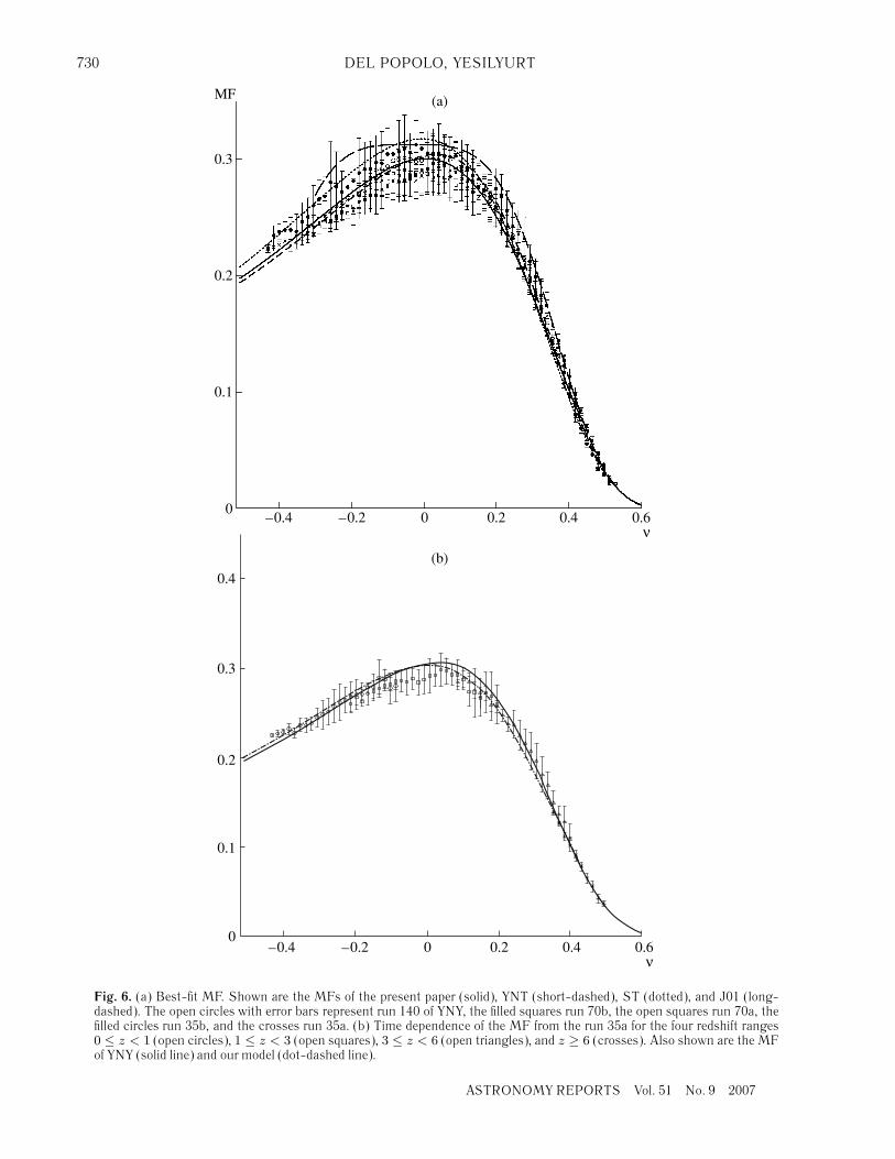
730 DEL POPOLO, YESILYURT
0.1
0.40
0.20–0.2–0.4
0.2
0.3
MF
0.6
ν
(a)
0.40.20–0.2–0.4 0.6
ν
0.3
0.2
0.1
0
0.4
(b)
Fig. 6. (a) Best-fit MF. Shown are the MFs of the present paper (solid), YNT (short-dashed), ST (dotted), and J01 (long-dashed). The open circles with error bars represent run 140 of YNY, the filled squares run 70b, the open squares run 70a, thefilled circles run 35b, and the crosses run 35a. (b) Time dependence of the MF from the run 35a for the four redshift ranges0 ≤ z < 1 (open circles), 1 ≤ z < 3 (open squares), 3 ≤ z < 6 (open triangles), and z ≥ 6 (crosses). Also shown are the MFof YNY (solid line) and our model (dot-dashed line).
ASTRONOMY REPORTS Vol. 51 No. 9 2007
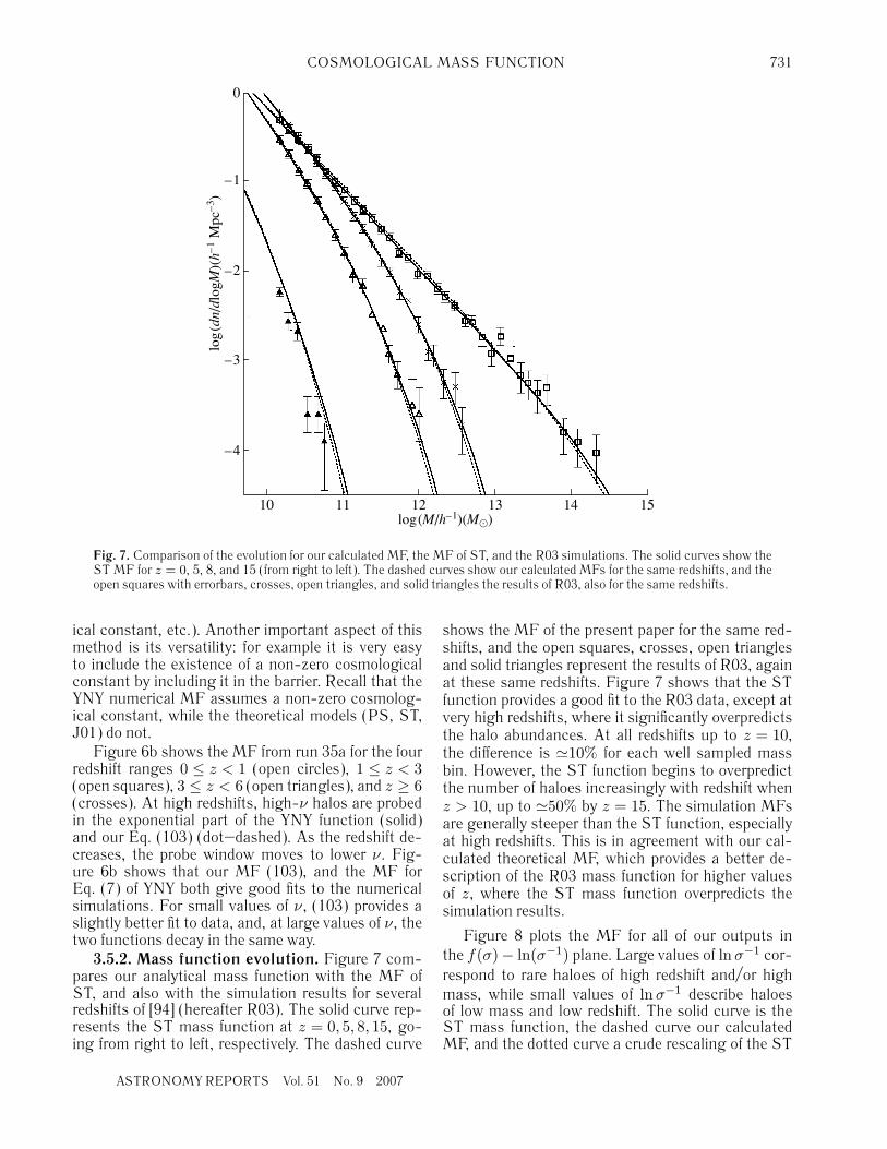
COSMOLOGICAL MASS FUNCTION 731
–4
10 11 12 13 14 15log(
M
/
h
–1
)(
M
�
)
–3
–2
–1
0
log
(
dn
/
d
log
M
)(
h
–1
Mpc
–3
)
Fig. 7. Comparison of the evolution for our calculated MF, the MF of ST, and the R03 simulations. The solid curves show theST MF for z = 0, 5, 8, and 15 (from right to left). The dashed curves show our calculated MFs for the same redshifts, and theopen squares with errorbars, crosses, open triangles, and solid triangles the results of R03, also for the same redshifts.
ical constant, etc.). Another important aspect of thismethod is its versatility: for example it is very easyto include the existence of a non-zero cosmologicalconstant by including it in the barrier. Recall that theYNY numerical MF assumes a non-zero cosmolog-ical constant, while the theoretical models (PS, ST,J01) do not.
Figure 6b shows the MF from run 35a for the fourredshift ranges 0 ≤ z < 1 (open circles), 1 ≤ z < 3(open squares), 3 ≤ z < 6 (open triangles), and z ≥ 6(crosses). At high redshifts, high-ν halos are probedin the exponential part of the YNY function (solid)and our Eq. (103) (dot–dashed). As the redshift de-creases, the probe window moves to lower ν. Fig-ure 6b shows that our MF (103), and the MF forEq. (7) of YNY both give good fits to the numericalsimulations. For small values of ν, (103) provides aslightly better fit to data, and, at large values of ν, thetwo functions decay in the same way.
3.5.2. Mass function evolution. Figure 7 com-pares our analytical mass function with the MF ofST, and also with the simulation results for severalredshifts of [94] (hereafter R03). The solid curve rep-resents the ST mass function at z = 0, 5, 8, 15, go-ing from right to left, respectively. The dashed curve
shows the MF of the present paper for the same red-shifts, and the open squares, crosses, open trianglesand solid triangles represent the results of R03, againat these same redshifts. Figure 7 shows that the STfunction provides a good fit to the R03 data, except atvery high redshifts, where it significantly overpredictsthe halo abundances. At all redshifts up to z = 10,the difference is �10% for each well sampled massbin. However, the ST function begins to overpredictthe number of haloes increasingly with redshift whenz > 10, up to �50% by z = 15. The simulation MFsare generally steeper than the ST function, especiallyat high redshifts. This is in agreement with our cal-culated theoretical MF, which provides a better de-scription of the R03 mass function for higher valuesof z, where the ST mass function overpredicts thesimulation results.
Figure 8 plots the MF for all of our outputs inthe f(σ)− ln(σ−1) plane. Large values of ln σ−1 cor-respond to rare haloes of high redshift and/or highmass, while small values of ln σ−1 describe haloesof low mass and low redshift. The solid curve is theST mass function, the dashed curve our calculatedMF, and the dotted curve a crude rescaling of the ST
ASTRONOMY REPORTS Vol. 51 No. 9 2007
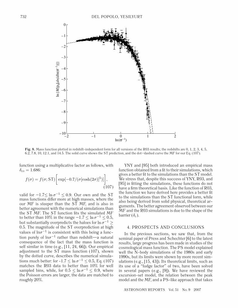
732 DEL POPOLO, YESILYURT
–9
–1–2 0 1 2ln(
σ
–1
)
–10
–8
–7
–6
–5
–4
–3
–2
–1
0
ln{
M
/
ρ
0
[
dn
/
dl
n(
σ
–1
)]}
Fig. 8. Mass function plotted in redshift-independent form for all versions of the R03 results; the redshifts are 0, 1, 2, 3, 4, 5,6.2, 7.8, 10, 12.1, and 14.5. The solid curve shows the ST prediction, and the dot–dashed curve the MF for our Eq. (107).
function using a multiplicative factor as follows, withδco = 1.686:
f(σ) = f(σ; ST)[
exp[−0.7/(σ[cosh(2σ)]5)]],
(107)
valid for –1.7≤ ln σ−1 ≤ 0.9. Our own and the STmass functions differ more at high masses, where theour MF is steeper than the ST MF, and is also inbetter agreement with the numerical simulations thanthe ST MF. The ST function fits the simulated MFto better than 10% in the range –1.7 ≤ lnσ−1 ≤ 0.5,but substantially overpredicts the haloes for ln σ−1 ≥0.5. The magnitude of the ST overprediction at highvalues of lnσ−1 is consistent with this being a func-tion purely of lnσ−1 rather than redshift—a naturalconsequence of the fact that the mass function isself similar in time (e.g., [11, 24, 66]). Our empiricaladjustment to the ST mass function (107), shownby the dotted curve, describes the numerical simula-tions much better: for -1.7 ≤ ln σ−1 ≤ 0.5, Eq. (107)matches the R03 data to better than 10% for wellsampled bins, while, for 0.5 ≤ ln σ−1 ≤ 0.9, wherethe Poisson errors are larger, the data are matched toroughly 20%.
YNY and [95] both introduced an empirical massfunction obtained from a fit to their simulations, whichgives a better fit to the simulations than the ST model.We stress that, despite this success of YNY, R03, and[95] in fitting the simulations, these functions do nothave a firm theoretical basis. Like the function of R03,the function we have derived here provides a better fitto the simulations than the ST functional form, whilealso being derived from solid physical, theoretical ar-guments. The better agreement observed between ourMF and the R03 simulations is due to the shape of thebarrier (δc).
4. PROSPECTS AND CONCLUSIONS
In the previous sections, we saw that, from theseminal paper of Press and Schechter [6] to the latestresults, large progress has been made in studies of thecosmological mass function. The PS model explainedwell the N-body simulations of the 1980s and early1990s, but its limits were shown by more recent sim-ulations (e.g., [15, 43]). Its theoretical limits, such asits use of a “fudge factor” of two, have been solvedin several papers (e.g., [9]). We have reviewed theexcursion-set model, the relation between the peakmodel and the MF, and a PS-like approach that takes
ASTRONOMY REPORTS Vol. 51 No. 9 2007
COSMOLOGICAL MASS FUNCTION 733
into account the dynamics in the MF theory. All thesestudies yielded MFs that were in better agreementwith the simulations, but only recently has it beenpossible to obtain MF functions that are in very goodagreement with the simulation results [6, 11, 13, 15,30, 49].
While the latest models for the mass function givemuch improved results over previous ones, it is nec-essary to recall the limitations of the theory and theproblems that remain to be attacked.
—More physics must be added to dynamical MFtheory, to describe events such as the aggregation andfragmentation of already collapsed structures. In thisway, the dynamics inside structures could be resolved;this is necessary to describe objects such as galaxiesinside larger structures, such as groups or clusters.The theories presented in the last subsection are ableto take account of some of these effects, such asfragmentation, angular-momentum acquisition, andthe existence of a non-zero cosmological constant.Changing the shape of the barrier provides a way totake into account more physical effects in dynamicalMF theory.
—The geometry of collapsed regions in Lagran-gian space must be more fully and accurately de-scribed, going beyond the usual golden rule describedabove. In the realistic case when the stochastic pro-cess on which the MF is based is not Gaussian, thiscan be performed via Monte Carlo simulations of theinitial fields.
—The role of filtering in the MF problem mustbe better understood, since different kinds of filters(sharp k-space, Gaussian) lead to different and notequivalent formulations of the problem.
—The total mass of a structure must be deter-mined in detail, and a rigorous, well-posed and easilyinterpretable definition for this mass defined, suitablefor use in interpreting observations. Another impor-tant point is connected to N-body simulations. Forexample, as was shown by YNY, there is a discrepancyin the numerical MFs from various simulation runs.There are three strategies to resolve this discrepancy.The first is to run simulations having still higher massdynamic ranges, free from the effect of the box size.The second is to increase the number of realizations,since there is scatter from the runs using the samebox size. The third is to run simulations whose boxsize is smaller than in the present work, although thismight sound contradictory. Simulations with smallerbox sizes can yield information about the conditionalMF, which coincides with the unconditional MF atν � 1. Comparing unconditional MFs from simula-tions with large box sizes and conditional MFs fromthose with small box sizes will offer clues to resolvethe above discrepancies, and may also provide in-sights into how the PS ansatz works to reproduce thenumerical MFs.
ACKNOWLEDGMENTS
The author thanks the referee M.V. Sazhin for hishelpful comments.
REFERENCES1. D. Sciama, Mon. Not. R. Astron. Soc. 244, 1 (1990).2. S. Bowyer, E. J. Korpela, J. Edelstein, et al., Astro-
phys. J. 526, 10 (1999).3. J. H. Oort, Bull. Astron. Inst. Netherlands 6, 249
(1932).4. F. Zwichy, Helv. Phys. Acta 6, 110 (1933).5. S. Smith, Astrophys. J. 83, 23 (1936).6. W. Press and P. Schechter, Astrophys. J. 187, 425
(1974).7. A. G. Doroshkevich, Astrophys. 3, 84 (1967).8. P. L. Schechter, Astrophys. J. 203, 297 (1976).9. J. R. Bond, S. Cole, G. Efstathiou, and N. Kaiser,
Astrophys. J. 379, 440 (1991).10. R. K. Sheth and G. Tormen, Mon. Not. R. Astron.
Soc. 308, 119 (1999).11. A. Jenkins, C. S. Frenk, S. D. M. White, et al., Mon.
Not. R. Astron. Soc. 321, 372 (2001).12. R. K. Sheth, H. J. Mo, and G. Tormen, Mon. Not. R.
Astron. Soc. 323, 1 (2001).13. R. K. Sheth and G. Tormen, Mon. Not. R. Astron.
Soc. 329, 61(ST) (2002).14. A. Del Popolo, Mon. Not. R. Astron. Soc. 337, 529
(2002).15. H. Yahagi, M. Nagashima, and Y. Yoshii, Astrophys.
J. 605, 709 (2004).16. G. Efstathiou, S. M. Fall, and C. Hogan, Astrophys.
J. 189, 203 (1979).17. R. Schaeffer and J. Silk, Astrophys. J. 292, 319
(1985).18. F. Lucchin, in Morphological Cosmology, Eds.
P. Flin, and H. W. Duerbeck (Springer Verlag, Berlin,1989).
19. A. Kashilinsky, Astrophys. J. 317, 19 (1987).20. E. Martinez-Gonzalez and J. L. Sanz, Astrophys. J.
324, 653 (1988).21. E. Martinez-Gonzalez and J. L. Sanz, Astrophys. J.
332, 89 (1988)22. F. Lucchin and S. Matarrese, Astrophys. J. 330, 535
(1988).23. P. B. Lilje, Astrophys. J. 386, L33 (1992).24. O. Lahav, P. B. Lilje, J. R. Primack, and M. J. Rees,
Mon. Not. R. Astron. Soc. 251, 128 (1991).25. Y. Zhan, Astrophys. J. 355, 387 (1990).26. R. Schaeffer and J. Silk, Astrophys. J. 332, 1 (1988).27. R. Schaeffer and J. Silk, Astrophys. J. 333, 509
(1988).28. F. Occhionero and R. Scaramella, Astron. Astrophys.
204, 3 (1988).29. C. Lacey and S. Cole, Mon. Not. R. Astron. Soc. 271,
676 (1994).30. A. Del Popolo and M. Gambera, Astron. Astrophys.
337, 96 (1998).31. G. Efstathiou, C. S. Frenk, S. D. M. White, and
M. Davis, Mon. Not. R. Astron. Soc. 235, 715 (1988).
ASTRONOMY REPORTS Vol. 51 No. 9 2007
734 DEL POPOLO, YESILYURT
32. G. Efstathiou and M. J. Rees, Mon. Not. R. Astron.Soc. 230, 5P (1988).
33. R. Narayan and S. D. M. White, Mon. Not. R. Astron.Soc. 231, 97P (1988).
34. R. G. Carlberg and H. M. P. Couchman, Astrophys.J. 340, 47 (1989).
35. R. G. Carlberg, Astrophys. J. 350, 505 (1990).36. S. D. M. White, G. Efstathiou, and C. S. Frenk, Mon.
Not. R. Astron. Soc. 262, 1023 (1993).37. B. Jain and E. Bertschinger, Astrophys. J. 431, 495
(1994).38. N. Katz, T. Quinn, E. Bertschinger, and J. M. Gelb,
Mon. Not. R. Astron. Soc. 270, L71 (1994).39. G. Efstathiou, Mon. Not. R. Astron. Soc. 272, L25
(1995).40. A. Klypin and G. Rhee, Astrophys. J. 428, 399 (1994).41. A. Klypin, S. Borgani, J. Holtzman, and J. Primack,
Astrophys. J. 444, 1 (1995).42. J. R. Bond and S. T. Myers, Astrophys. J., Suppl. Ser.
103, 1 (1996).43. F. Governato, P. Tozzi, and A. Cavaliere, Astrophys. J.
458, 18 (1996).44. T. G. Brainerd and J. V. Villumsen, Astrophys. J. 394,
409 (1992).45. J. M. Gelb and E. Bertschinger, Astrophys. J. 436,
467 (1994).46. C. Ma and E. Bertschinger, Astrophys. J. 434, L5
(1994).47. P. Monaco, Fundam. Cosm. Phys. 19, 153 (1998).48. A. Del Popolo, Mon. Not. R. Astron. Soc. 336, 81
(2002).49. A. Del Popolo and M. Gambera, Astron. Astrophys.
344, 17 (1999).50. A. Friedmann, Z. Phys. 10, 377 (1924).51. A. Friedmann, Z. Phys. 21, 326 (1924).52. A. Einstein, Preuss. Akad. Wiss. Berlin, Sitzber., 844
(1915).53. P. J. E. Peebles, The Large Scale Structure of the
Universe (Princeton Univ. Press, Princeton, 1980).54. Ya. B. Zel’dovich, Astron. Astrophys. 5, 84 (1970).55. J. E. Gunn and J. R. Gott, Astrophys. J. 176, 1
(1972).56. F. Bernardeau, Astron. Astrophys. 291, 697 (1994).57. G. F. R. Ellis, in General Relativity and Cosmology
Ed. by R. K. Sachs (Academic Press, New York,1971).
58. T. Buchert, Mon. Not. R. Astron. Soc. 254, 729(1992).
59. G. Efstathiou, in The Physics of the Early Uni-verse, Ed. by A. Heavens, J. Peacock, and A. Davies(SUSSP, 1990).
60. G. Efstathiou and J. Silk, Fundam. Cosm. Phys. 9, 1(1983).
61. S. N. Gurbatov, A. I. Saıchev, and S. N. Shandarin,Dokl. Akad. Nauk SSSR 285, 323 (1985).
62. T. Watanabe and S. Inagaki, Publ. Astron. Soc. Jpn.43, 413 (1991).
63. D. J. Eisenstein and A. Loeb, Astrophys. J. 439, 520(1995).
64. B. S. Ryden, Astrophys. J. 329, 589 (1988).65. P. B. Lilje, A. Yahil, and B. J. T. Jones, Astrophys. J.
297, 27 (1986).
66. G. Efstathiou, C. S. Frenk, S. D. M. White, andM. Davis, Mon. Not. R. Astron. Soc. 235, 715 (1988).
67. S. D. M. White and C. S. Frenk, Astrophys. J. 379,52 (1991).
68. P. Tozzi and F. Governato, in The Young Universe:Galaxy Formation and Evolution at Intermediateand High Redshift, Ed. by S. D’Odorico, A. Fontana,and E. Giallongo, Astron. Soc. Pac. Conf. Ser. 146,461 (1988).
69. J. A. Peacock and A. F. Heavens, Mon. Not. R. As-tron. Soc. 243, 133 (1990).
70. R. Adler, The Geometry of Random Fields (Wiley,New York, 1981).
71. C. Lacey and S. Cole, Mon. Not. R. Astron. Soc. 262,627 (1993).
72. J. M. Bardeen, J. R. Bond, N. Kaiser, and A. S. Sza-lay, Astrophys. J. 304, 15 (1986).
73. S. Cole, Astrophys. J. 367, 45 (1991).74. S. Chandrasekhar and J. von Neumann, Astrophys. J.
97, 1 (1943).75. R. G. Bower, Mon. Not. R. Astron. Soc. 248, 332
(1991).76. R. K. Sheth, Mon. Not. R. Astron. Soc. 276, 796
(1995).77. R. K. Sheth, Mon. Not. R. Astron. Soc. 281, 1277
(1996).78. A. G. Doroshkevich, Astrofizika 6, 581 (1970) [Astro-
phys. 6, 320 (1970)].79. N. Kaiser, Astrophys. J. 284, L9 (1984).80. J. A. Peacock and A. F. Heavens, Mon. Not. R. As-
tron. Soc. 217, 805 (1985).81. N. Katz, T. Quinn, and J. M. Gelb, Mon. Not. R.
Astron. Soc. 265, 689 (1993).82. R. van de Weygaert and A. Babul, Astrophys. J. 425,
L59 (1994).83. A. Manrique and E. Salvador-Sole, Astrophys. J.
453, 6 (1995).84. J. R. Bond and S. T. Myers, Astrophys. J., Suppl. Ser.
103, 41 (1996).85. J. R. Bond, in Large-Scale Motions in the Universe,
Ed. by V. Rubin and G. Coyne (Princeton Univ. Press,Princeton, 1989).
86. Y. Hoffman, Astrophys. J. 329, 8 (1988).87. S. Colafrancesco, F. Lucchin, and S. Matarrese, As-
trophys. J. 345, 3 (1989).88. P. J. E. Peebles, Principles of Physical Cosmology
(Princeton Univ. Press, Princeton, 1993).89. A. Del Popolo, E. N. Ercan, and Z. Q. Xia, Astron. J.
122, 487 (2001).90. N. A. Bahcall and X. Fan, Astrophys. J. 504, 1 (1998).91. P. Monaco, Mon. Not. R. Astron. Soc. 287, 753
(1997).92. P. Monaco, Mon. Not. R. Astron. Soc. 290, 439
(1997).93. Y. Hoffman, Astrophys. J. 308, 493 (1986).94. D. Reed, J. Gardner, Th. Quinn, et al., Mon. Not. R.
Astron. Soc. 346, 565 (2003).95. M. S. Warren, K. Abazajian, D. E. Holz, and
L. Teodoro, astro-ph/0506395 (2005).
ASTRONOMY REPORTS Vol. 51 No. 9 2007
Related Documents