THE COSMIC NEAR-INFRARED BACKGROUND. II. FLUCTUATIONS

arX

iv:0

906.

4552

v2 [

astr

o-ph

.CO

] 7

Jan

201

0

THE COSMIC NEAR INFRARED BACKGROUND II:

FLUCTUATIONS

Elizabeth R. Fernandez1, Eiichiro Komatsu2, Ilian T. Iliev3,4, Paul R. Shapiro2

1Center for Astrophysics and Space Astronomy, University of Colorado, 389 UCB,

Boulder, CO 80309-03892Texas Cosmology Center and the Department of Astronomy, The University of Texas at

Austin, 1 University Station, C1400, Austin, TX 787123Astronomy Centre, Department of Physics & Astronomy, Pevensey II Building, University

of Sussex, Falmer, Brighton BN1 9QH, United Kingdom4Universitat Zurich, Institut fur Theoretische Physik, Winterthurerstrasse 190, CH-8057

Zurich, Switzerland

[email protected]

ABSTRACT

The Near Infrared Background (NIRB) is one of a few methods that can be

used to observe the redshifted light from early stars at a redshift of six and above,

and thus it is imperative to understand the significance of any detection or non-

detection of the NIRB. Fluctuations of the NIRB can provide information on the

first structures, such as halos and their surrounding ionized regions in the Inter

Galactic Medium (IGM). We combine, for the first time, N -body simulations,

radiative transfer code, and analytic calculations of luminosity of early structures

to predict the angular power spectrum (Cl) of fluctuations in the NIRB. We study,

in detail, the effects of various assumptions about the stellar mass, the initial

mass spectrum of stars, metallicity, the star formation efficiency (f∗), the escape

fraction of ionizing photons (fesc), and the star formation timescale (tSF), on the

amplitude as well as the shape of Cl. The power spectrum of NIRB fluctuations

is maximized when f∗ is the largest (as Cl ∝ f 2∗) and fesc is the smallest (as

more nebular emission is produced within halos). A significant uncertainty in

the predicted amplitude of Cl exists due to our lack of knowledge of tSF of these

early populations of galaxies, which is equivalent to our lack of knowledge of

the mass-to-light ratio of these sources. We do not see a turnover in the NIRB

angular power spectrum of the halo contribution, which was claimed to exist in

the literature, and explain this as the effect of high levels of non-linear bias that

was ignored in the previous calculations. This is partly due to our choice of the

– 2 –

minimum mass of halos contributing to NIRB (∼ 2 × 109 M⊙), and a smaller

minimum mass, which has a smaller non-linear bias, may still exhibit a turn

over. Therefore, our results suggest that both the amplitude and shape of the

NIRB power spectrum provide important information regarding the nature of

sources contributing to the cosmic reionization. The angular power spectrum of

the IGM, in most cases, is much smaller than the halo angular power spectrum,

except when fesc is close to unity, tSF is longer, or the minimum redshift at which

the star formation is occurring is high. In addition, low levels of the observed

mean background intensity tend to rule out high values of f∗ & 0.2.

Subject headings: cosmology: theory — diffuse radiation — galaxies: high-

redshift — infrared: galaxies

1. INTRODUCTION

We have few probes of the early universe and the first few generations of stars. We

know that stars had to form early in order to pollute the universe with metals and reion-

ize the universe. There is evidence that the universe was reionized at around z ∼ 11,

such as from the Wilkinson Microwave Anisotropy Probe (WMAP) satellite (Kogut et al.

2003; Spergel et al. 2003, 2007; Page et al. 2007; Dunkley et al. 2009; Komatsu et al. 2009).

Stars are efficient producers of ionizing photons, so are likely candidates for the bulk of

reionization. These ultraviolet photons at redshifts 6 . z . 30 would be redshifted

into the near-infrared bands. Therefore, it makes sense to search for this remnant light

in the near infrared bands to learn about this early epoch of star formation and reion-

ization (Santos, Bromm & Kamionkowski 2002; Magliocchetti, Salvaterra, & Ferrara 2003;

Salvaterra & Ferrara 2003; Cooray et al. 2004; Cooray & Yoshida 2004; Kashlinsky et al.

2004; Madau & Silk 2005; Fernandez & Komatsu 2006). Observations of the Near Infrared

Background (NIRB) may indicate that there is an excess mean background above that normal

galaxies can account for (Dwek & Arendt 1998; Gorjian, Wright & Chary 2000; Kashlinsky & Odenwald

2000; Wright & Reese 2000; Wright 2001; Cambresy et al. 2001; Totani et al. 2001; Matsumoto et al.

2005; Kashlinsky 2005). In addition, there also appears to be a peak in the NIRB spectrum

at 1–2 µm, which could represent a Lyman-cutoff signature (Bock et al. 2006). However, the

interpretation of the current observational data, in particular accuracy of the subtraction

of Zodiacal light and foreground galaxies, is highly controversial (Thompson et al. 2007a,b).

Nevertheless, any detection or non-detection of this excess light could tell us properties of

early stars.

In addition to the mean intensity, fluctuations in the NIRB can provide an additional

– 3 –

source of information about the first generations of stars (Kashlinsky & Odenwald 2000;

Kashlinsky et al. 2002, 2004, 2005, 2007a,b,c; Kashlinsky 2005; Magliocchetti, Salvaterra, & Ferrara

2003; Odenwald et al. 2003; Cooray et al. 2004; Matsumoto et al. 2005; Thompson et al.

2007a,b). Fluctuations are in general easier to study than the mean intensity because

an accurate determination of the zero point is not needed; thus, they are less sensitive

to the imperfect subtraction of Zodiacal light. However, as the contribution to fluctua-

tions from low redshift populations, i.e., z < 6, can confuse the signal from higher red-

shift populations, the level of contamination from low redshift populations must be esti-

mated and subtracted carefully (Sullivan et al. 2007; Cooray et al. 2007; Kashlinsky et al.

2007c; Thompson et al. 2007b; Chary, Cooray & Sullivan 2008). Upcoming measurements

with AKARI (Matsuhara et al. 2008) and CIBER (the Cosmic Infrared Background Exper-

iment) (Bock et al. 2006; Cooray et al. 2009) may be able to put a more solid constraint on

what fraction of the NIRB is from high redshift stars and galaxies.

In the previous paper we have presented detailed theoretical calculations of the spectrum

and metallicity/initial-mass-spectrum dependence of the mean intensity of NIRB (Fernandez & Komatsu

(2006), hereafter FK06). In this paper we present calculations of the power spectrum and

metallicity/initial-mass-spectrum dependence of the NIRB fluctuations, as well as depen-

dence on the star formation efficiency and the escape fraction of ionizing photons. While

the previous work in the literature (Cooray et al. 2004; Kashlinsky et al. 2004) relied solely

on simplified analytical arguments, we use, for the first time, large-scale cosmological sim-

ulations of cosmic reionization given in Iliev et al. (2006, 2007, 2008b), coupled with the

analytical calculations given in FK06, to predict the power spectrum of NIRB fluctuations.

In this way we are able to capture the contribution from ionized bubbles surrounding the

halos, which has been ignored completely in the previous work.

In § 2 we outline the simulations (Iliev et al. 2006, 2007, 2008b) and in § 3 we explain the

analytic formulas we use to obtain the luminosity of the halos and the surrounding IGM. In

§ 4 we present our calculation of the luminosity-density power spectrum, PL(k). Predictions

for PL(k) and the angular power spectrum of NIRB fluctuations, Cl, are presented in § 5.

Various parameters’ effects on the results are discussed in § 6. We compare our results to the

previous literature in § 7 and to observations in § 8. We take a look at the constraints from

the mean NIRB in § 9, and compute the fractional anisotropy, i.e., the ratio of the power

spectrum and the mean intensity squared, in § 10. We conclude in § 11.

– 4 –

2. SIMULATION

We use simulations from Iliev et al. (2006, 2007, 2008b), which are the first truly large

scale simulations to include radiative transfer, and are therefore ideal for predicting the

distribution of luminosities from high redshift stellar populations. Simulations provide the

advantage of being able to simultaneously model the distribution of halos and the density of

the IGM, as well as the ionization front that propagates through the IGM. We combine this

N -body code with radiative transfer and analytic formulas for luminosity to simulate their

luminosity-density power spectrum.

The particular simulation that we use in this paper is the run “f250C” in Table I of

Iliev et al. (2008b), which was run with the cosmological parameters given by the WMAP

3-year results (Spergel et al. 2007), (Ωm, ΩΛ, Ωb, h, σ8, ns)=(0.24, 0.76, 0.042, 0.73, 0.74,

0.95). Aside from the cosmological parameters, the only free parameter in the reionization

simulation of this kind is the production rate of ionizing photons escaping into the IGM per

halo. We shall come back to this parameter, called fγ/tSF, in § 3.2.

These simulations combine a high resolutionN -body code (PMFAST, see Merz, Pen & Trac

2005) with a radiative transfer code (C2-Ray, see Mellema et al. 2006), which is a conserva-

tive, causal ray-tracing radiative transfer code. The C2-Ray code traces the ionization front

by tracking photons using photon conservation. The code allows for large time steps and

coarse grids without loss of accuracy.

The box size of the simulation is 100 h−1 Mpc, which is large enough to sample the

history, geometry, and statistical properties of reionization. The number of particles is 16243,

and the density field was sampled on a lattice of 32483 cells. The density field was then binned

to 2033 cells for the radiative transfer calculations. We use the 2033 cells when we compute

the radiation from the IGM in § 4.2. The minimum mass of the halos is 2.2×109 M⊙, which

represents dwarf galaxies. These halos have virial temperatures of 1.2× 104 K, 1.8× 104 K,

and 2.6 × 104 K at z = 6, 10, and 15 respectively. For these halos the dominant cooling

process is hydrogen atomic cooling. It is important to sample these dwarf galaxies, as they

are far more numerous than larger galaxies and may provide most of the photons needed for

reionization.

Even though this simulation is a very powerful tool, it is important to consider its

limitations. Halos slightly below the resolution of this simulation (108 to 109 M⊙) may

also be an important source for ionizing radiation. Iliev et al. (2007) also did a smaller

box-size simulation [(35 h−1 Mpc)3] that resolves halos down to 108 M⊙, which includes

halos that form stars as a result of atomic cooling. These smaller halos allow the ionization

fraction to reach 50% at an earlier epoch than the simulations that only resolved down to

– 5 –

2.2× 109 M⊙. However, Iliev et al. (2007) found that the redshift in which reionization was

completed remained about the same for the 100 h−1 Mpc and 35 h−1 Mpc simulations, due

to the “self-regulation” (see Iliev et al. 2007, for details).

The results discussed in this paper are based on the larger box size with halos resolved

down to 2.2×109 M⊙. It is possible that the smaller halos would affect the fluctuations in the

NIRB from both the halos and the IGM. Future simulations will allow both a larger box size

along with a smaller minimum mass. These future simulations will be able to provide more

robust predictions for the fluctuations in the NIRB if these smaller halos contribute to the

NIRB. Simulations that resolve halos smaller than 108 M⊙ may not be needed, however: while

these minihalos were likely the sites of the truly first generation of stars, they may not be a

significant source of ionizing photons to reionize the universe, as UV photons in the Lyman

Werner bands dissociate molecular hydrogen, terminating star formation in these small halos

(Haiman, Rees & Loeb 1997; Haiman, Abel & Rees 2000; Machacek, Bryan & Abel 2003;

Yoshida et al. 2003; Johnson, Grief & Bromm 2008; Ahn et al. 2009). However, there is

on-going discussion as to what the radiation feedback actually does for the formation of

second generation stars (Wise et al. 2007; Ahn & Shapiro 2007; O’Shea & Norman 2008).

While the Lyman Werner background from early star formation has a primarily negative

feedback effect, other processes (e.g., cooling in supernova remnant shocks) may mitigate

the suppression of H2 molecules (Ferrara 1998; Ricotti et al. 2001).

3. ANALYTICAL CALCULATION

In this section we describe how we assign the luminosity to the halos and the IGM in

the simulation. Note that our method is fully analytical, and thus can be adopted to any

other reionization simulations.

3.1. Luminosity of the halos

Luminosity within the halos is dominated by five radiative processes: stellar (black-

body) emission, and the nebular emission including free-free, free-bound, and two-photon

emission, as well as any emission lines (here, Lyman-α is the most important one for our study

of NIRB). The luminosity of each component can be found analytically using the equations

in FK06. Equations for the stars’ luminosity, temperature, number of ionizing photons per

second, and lifetime were based on equations from Table 3 of Fernandez & Komatsu (2008),

which were fit from stellar models or fitting functions (Marigo et al. 2001; Lejeune & Schaerer

– 6 –

2001; Schaerer 2002).

First, let us define the “volume emissivity.” The volume emissivity (luminosity per

comoving volume per frequency), p(ν), is related to the “emission coefficient” (luminosity

per comoving volume per frequency per steradian), jν , in Santos, Bromm & Kamionkowski

(2002); Cooray et al. (2004) by p(ν) = 4πjν . In other words, the luminosity is given by

dL = p(ν)dνdV = jνdΩdνdV, (1)

where dV is the comoving volume element, and dΩ is the solid angle element. Integrating

p(ν) over ν, one obtains the “comoving luminosity density,” ρL, as dL = ρLdV , where

ρL =∫p(ν)dν.

When the main-sequence lifetime of stars under consideration is shorter than the time

scale at which the star formation takes place, the volume emissivity is given by a product

of the star formation rate (the stellar mass density formed per unit time), ρ∗(z), and the

ratio of the mass-weighted average of the total radiative energy (including stellar emission

and reprocessed light) emitted over the stellar lifetime to the stellar rest-mass energy, 〈ǫαν 〉

(see Eq. (2) of FK06):

p(ν, z) =∑

α

pα(ν, z) = ρ∗(z)c2∑

α

〈ǫαν 〉, (2)

where

〈ǫαν 〉 =

∫ m2

m1dm [Lα

ν (m)τ(m)/(mc2)] f(m)m∫ m2

m1dmf(m)m

. (3)

Here, m is the stellar mass, Lαν (m) is the time-averaged luminosity per frequency of a given

radiative process α (which includes the stellar, free-free, free-bound, two-photon, and Lyman-

α emission), τ(m) is the main sequence lifetime, and f(m) is the initial mass spectrum of

stars under consideration (specified later in § 3.2). Note that 〈ǫαν 〉 may also be interpreted

as a ratio of the total radiative energy within a unit frequency to the total stellar rest-mass

energy,

〈ǫαν 〉 =

∫ m2

m1dmf(m)Lα

ν (m)τ(m)∫ m2

m1dmf(m)mc2

. (4)

Either way, 〈ǫαν 〉 is a convenient quantity that tells us how much of the stellar rest-mass

energy is converted into the radiative energy within a unit frequency interval.

In FK06 we have shown that 〈ǫαν 〉 can be calculated robustly for a given stellar popu-

lation, i.e., f(m), using the basic stellar physics and radiative processes in the interstellar

medium. For the radiative processes and stellar populations we consider in this paper,

– 7 –

ν〈ǫαν 〉 . 10−3 (see Figure 2 of FK06). From this one may obtain a quantity that is commonly

used in the literature, the luminosity per stellar mass, lαν , as

lαν (z) =pα(ν, z)

ρ∗(z)=

d ln ρ∗(z)

dt

∫ m2

m1dmf(m)Lα

ν (m)τ(m)∫ m2

m1dmf(m)m

. (5)

In this expression one may identify d ln ρ∗(z)/dt as the inverse of the star formation timescale,

tSF(z), i.e., tSF(z) ≡ [d ln ρ∗(z)/dt]−1.1 Therefore, we finally obtain

lαν (z) =1

tSF(z)

∫ m2

m1dmf(m)Lα

ν (m)τ(m)∫ m2

m1dmf(m)m

, (6)

when the main sequence lifetime of stars is shorter than the star formation timescale, τ(m) <

tSF(z). In terms of 〈ǫαν 〉 we may also write Eq. (6) as lαν (z) = 〈ǫαν 〉c2/tSF(z).

On the other hand, when the star formation timescale is shorter than the main sequence

lifetime of stars, tSF(z) < τ(m), we find a different expression for lαν (see Eq. (A6) of FK06):

lαν =

∫ m2

m1dmf(m)Lα

ν (m)∫ m2

m1dmf(m)m

, (7)

and lαν no longer depends on z as long as f(m) does not depend on z. From Eqs. (6) and (7)

we find that the former is roughly τ/tSF times the latter. In other words, if one misused the

latter form when τ < tSF, one would over-estimate the signal by a factor of ≈ tSF/τ , which

can be as large as a factor of 10 for short-lived, massive stars with ∼ 100 M⊙.2

For the precise calculation one should use both expressions depending on the situation;

however, to simplify the analysis, we shall use either Eq. (6) or (7), depending on the ratio

of the stellar lifetime averaged over the initial mass spectrum and weighted by the luminos-

ity (since more massive, shorter lived stars will contribute more to the overall luminosity),

〈τ〉 ≡∫ m2

m1dmf(m)τ(m)L/

∫ m2

m1dmf(m)L, to the star formation timescale (where L is the

1If one assumes that the star formation is triggered by mergers of dark matter halos,

then the star formation timescale may be related to the halo merger rate, i.e., t−1

SF(z) =

[∫dMhMh(d

2nh/dMhdt)]/[∫dMhMh(dnh/dMh)], where dnh/dMh is the mass function of dark matter halos.

This approach was used by Santos, Bromm & Kamionkowski (2002); Cooray et al. (2004); Cooray & Yoshida

(2004). In this paper we shall use tSF = 20 Myr as our fiducial value, to be consistent with the value used

by the simulation of Iliev et al. (2008b). We also study the effects of changing tSF in § 6.1.

2Salvaterra & Ferrara (2003); Magliocchetti, Salvaterra, & Ferrara (2003); Kashlinsky et al. (2004) used

Eq. (7) for τ < tSF, and thus their predicted amplitudes of NIRB are likely over-estimated by a factor of

≈ tSF/τ .

– 8 –

bolometric luminosity). In the simulations of Iliev et al. (2006, 2007, 2008b), the star forma-

tion timescale takes on a universal value, tSF ≈ 20 Myr. For all the stellar populations, the

luminosity-weighted lifetime is shorter than 20 Myr; thus, Eq. 7 will be our fiducial formula.

To compute lαν for each radiative process, we use a black-body for the stellar component,

l∗ν (see Eq. (6) of FK06). This emission is cutoff above 13.6 eV, so all of the ionizing photons

go into producing emission in the nebula or the IGM. The expressions given in § 2.3, 2.4,

and 2.5 of FK06 are used for the nebular processes. We then integrate lαν over a band of

observed frequencies ν1 to ν2 to obtain the band-averaged luminosity per stellar mass, lα, as

lα(z) ≡

∫ ν2(1+z)

ν1(1+z)

dν lαν (z). (8)

Following Iliev et al. (2006, 2007, 2008b), we assume all halos have a constant mass-to-

light ratio. With the luminosities per stellar mass, lα(z), computed, we obtain the luminosi-

ties of the halo, Lh(z), by multiplying l(z) by the total stellar mass per halo, f∗Mh(Ωb/Ωm),

where Mh is the total halo mass (including dark matter and baryons), and f∗ is the star

formation efficiency, which is the fraction of baryons that can form into stars over the star

formation timescale tSF. We find

Lh(z)

Mh= f∗

Ωb

Ωm

l∗(z) + (1− fesc)

[lff (z) + lfb(z) + l2γ(z) + lLyα(z)

], (9)

where fesc is the escape fraction of ionizing photons from the halo. Only those photons that

do not escape into the IGM produce nebular emission within the halo.

From this result one may conclude immediately that the NIRB power spectrum from

halos, which is proportional to (Lh/Mh)2, is proportional to f 2

∗. Also, Lh/Mh goes down

as fesc approaches unity, for which all the ionizing photons would escape halos, and thus

no nebular emission would be left in halos. The stellar properties, such as metallicities and

initial mass spectra, affect only lα.

3.2. Stellar Populations

The simulations from Iliev et al. (2008b) define a quantity, fγ , which is proportional to

the number of ionizing photons that escape into the IGM:

fγ = f∗fescNi, (10)

where Ni is the number of ionizing photons emitted per stellar atom. When modeling stellar

populations in our calculations, we shall assure that each of our models agrees with fγ = 250,

which was used in the simulations.

– 9 –

Population Initial Mass Spectrum m1, m2 〈τ〉 (Myr) Ni fesc f∗Pop III Salpeter 3M⊙, 150M⊙ 8.08 5600 0.22 0.2

Pop III Larson, mc = 250M⊙ 3M⊙, 500M⊙ 2.45 25000 0.1 0.1

Pop III Salpeter 3M⊙, 150M⊙ 8.08 5600 0.9 0.05

Pop III Larson, mc = 250M⊙ 3M⊙, 500M⊙ 2.45 25000 1 0.01

Pop II Salpeter 3M⊙, 150M⊙ 9.04 2600 0.95 0.1

Pop II Larson, mc = 50M⊙ 3M⊙, 150M⊙ 4.87 12000 0.9 0.023

Pop II Salpeter 3M⊙, 150M⊙ 9.04 2600 0.19 0.5

Pop II Larson, mc = 50M⊙ 3M⊙, 150M⊙ 4.87 12000 0.098 0.21

Table 1: Stellar populations (“Pop III” are metal-free, and “Pop II” are metal-poor with the

metallicity of Z = 1/50 Z⊙), parameters for initial mass spectra, the luminosity-weighted

main sequence lifetime of stars (〈τ〉), the corresponding number of ionizing photons per stellar

atom (Ni), escape fractions of ionizing photons (fesc), and the star formation efficiency (f∗).

Note that fesc and f∗ are tuned such that the value of fγ = fescf∗Ni is held fixed at fγ = 250

which, when combined with the star formation timescale of tSF = 20 Myr, can reionize

the universe such that the resulting electron-scattering optical depth is consistent with the

WMAP data.

Iliev et al. (2008b) have shown that this choice of fγ , combined with the universal star

formation timescale of tSF = 20 Myr, can reionize the universe successfully with the resulting

electron-scattering optical depth consistent with the WMAP data. Within this framework,

since fγ/tSF is the only free parameter, models with the same fγ/tSF would produce the

same reionization histories. (For the simulation case f250C on which our calculations here

are based, for example, the globally-averaged ionized fraction of the IGM was found to be

50% at z = 8.3 and 99% at z = 6.6.) To keep fγ/tSF constant, the star formation efficiency

must decrease as the escape fraction increases. The various populations that were modeled

are shown in Table 1.

We modeled both zero metallicity stars (Population III; Z = 0) and low metallicity

stars (Population II; Z = 1/50 Z⊙) with either a heavy or a light initial mass spectrum,

accompanied with either a low escape fraction (fesc ∼ 0.1) or a high escape fraction (fesc ∼ 1).

While we try to simulate a range of parameters, it is good to keep in mind that our choice of

f∗ and fesc for a given fγ is basically arbitrary. The level of NIRB fluctuations can change

significantly when paired with different assumptions for the metallicity, mass, and values for

fesc and f∗.

A lighter mass distribution of stars is represented by a Salpeter initial mass spectrum

– 10 –

(Salpeter 1955)

f(m) ∝ m−2.35. (11)

We use mass limits of m1 = 3M⊙ and m2 = 150M⊙ for this spectrum. Heavier stars are

represented by a Larson initial mass spectrum (Larson 1998)

f(m) ∝ m−1

(1 +

m

mc

)−1.35

, (12)

with m1 = 3M⊙, m2 = 500M⊙, and mc = 250M⊙ for Population III stars and m1 = 3M⊙,

m2 = 150M⊙, and mc = 50M⊙ for Population II stars.

In Figure 1 we show νlαν (in units of nW M−1⊙ ), and in Figure 2 we show lα(z) (in units

of nW M−1⊙ ) averaged over a rectangular bandpass from 1−2 µm, for the stellar populations

we consider in this paper. In the relevant redshift range, 7 . z . 15, the stellar, two-photon,

and Lyα emission are the most dominant radiation processes, and all of them are on the

order of l ∼ 1038 nW M−1⊙ (20 Myr/tSF).

3.3. Luminosity Density from IGM

Photons that do escape the halos go into producing emission in the HII region surround-

ing the halo in the IGM (free-free, free-bound, two photon and Lyman-α emission). The

emission in the HII region can be found using the volume emissivity, p(ν), i.e., luminosity

per comoving volume per frequency, or luminosity density per frequency (see Eq. (1) for the

precise definition).

Since all of the radiative processes we discuss in this section are proportional to the

number density squared, we need to be careful about the comoving versus proper quantities.

The proper volume emissivity is proportional to the proper number density squared, i.e.,

pprop ∝ n2prop. As the comoving volume emissivity is pcom = a3pprop = pprop/(1 + z)3 and the

comoving number density is ncom = a3nprop = nprop/(1 + z)3, we obtain pcom ∝ (1 + z)3n2com.

This factor of (1 + z)3 simply reflects the fact that the IGM was denser at higher redshift,

and thus the IGM was brighter. In the following derivations n always refers to the comoving

number density.

For free-free and free-bound emission, the volume emissivity is

pff,fb(ν, z) = 4π(1 + z)3nenpγce−hν/kTg

T1/2g

, (13)

where ne and np are the comoving number density of electrons and protons respectively, γc

– 11 –

Fig. 1.— Luminosity spectrum per stellar mass. The stellar, νl∗ν (triple-dot dashed red line),

free-free, νlffν (dotted purple line), free-bound, νlfbν (dashed light blue line), two-photon,

νl2γν (dot dashed green line), and Lyman-α emission, νlLyαν (solid dark blue line), are shown

in units of nW M−1⊙ as a function of the rest-frame energies. The stars are at z = 10, but

the redshift affects the profile of the Lyman-α line only, which was taken from Eq. (15) of

Santos, Bromm & Kamionkowski (2002).

– 12 –

Fig. 2.— Luminosity per stellar mass averaged over a rectangular bandpass from 1− 2 µm.

The stellar, l∗ (triple-dot dashed red line), free-free, lff (dotted purple line), free-bound, lfb

(dashed light blue line), two-photon, l2γ (dot dashed green line), and Lyman-α emission, lLyα

(solid dark blue line), are shown in units of nW M−1⊙ as a function of redshifts. Free-free

and free-bound both decrease with redshift. This is because both decrease with energy, and

as redshift is increased, the bandwidth corresponds to higher rest-frame energies. The initial

rise in Lyman-α is due to the wing of the line. At z ∼ 15.5, the line hits the end of the band

where there is no more Lyman-α emission. Stellar emission increases initially because there

is more emission from the star as energy increases, and later decreases as the bandwidth

begins to sample energies above 13.6 eV. Two photon emission is cut off at z ∼ 15.5, which

corresponds to the band sampling above 10.2 eV, above which there is no emission.

– 13 –

is the continuum emission coefficient including free-free and free-bound emission:

γc ≡ fk

[gff +

∞∑

n=2

xnexn

ngfb(n)

], (14)

where xn ≡ Ry/(kTgn2), gff and gbf(n) are the Gaunt factors for free-free (which is thermally

averaged) and free-bound emission, respectively, fk is the collection of physical constants

which has a numerical value of 5.44 × 10−39 in cgs units, and Tg is the gas temperature,

which we took to be 104 K (see § 2.3 of FK06 for more details).

Using the charge neutrality, ne = np, we write

nenp = n2e = n2

HX2e , (15)

where nH is the number density of hydrogen atoms and Xe is the ionization fraction, both

of which are given in the simulation. The volume emissivity is therefore given by

pff,fb(ν, z)

n2HX

2e

= 4π(1 + z)3γce−hν/kTg

T1/2g

. (16)

The two-photon emissivity is

p2γ(ν, z) = (1 + z)32hν

νLyαP (y)(1− fLyα)αBnenp, (17)

A fraction of photons that make the 2−1 transition, (1−fLyα), go into two photon emission,

while the remainder, fLyα, produce the Lyman-α line. The precise value of fLyα depends

slightly on the temperature of gas, and for a gas at 104 K the value of fLyα is 0.64 (Spitzer

1978). Here, αB is the case B hydrogen recombination coefficient given by

αB =2.06× 10−11

T1/2g

φ(Tg) cm3 s−1, (18)

where φ(Tg) is given by Spitzer (1978). Here, P (y) is the normalized probability per two

photon decay that one photon is in the range dy = dν/νLyα, which can be fit as (Eq. (22) of

FK06)

P (y) = 1.307− 2.627(y − 0.5)2 + 2.563(y − 0.5)4 − 51.69(y − 0.5)6, (19)

and νLyα is the frequency of Lyman-α photons. Using nH and Xe, we write the emissivity as

p2γ(ν, z)

n2HX

2e

= (1 + z)32hν

νLyαP (y)(1− fLyα)αB. (20)

– 14 –

For Lyman-α,

pLyα(ν, z) = (1 + z)3fLyαhνLyαnenpαBφ(ν − νLyα), (21)

where φ(ν − νLyα) is the line profile of the Lyman-α line, given in Loeb & Rybicki (1999);

Santos, Bromm & Kamionkowski (2002). Using nH and Xe, we get

pLyα(ν, z)

n2HX

2e

= (1 + z)3fLyαhνLyααBφ(ν − νLyα). (22)

Collecting all the processes we obtain the volume emissivity of the IGM as

pIGM(ν, z)

n2HX

2e

= (1+z)3

4πγc

e−hν/kTg

T1/2g

+ αBhνLyα

[(1− fLyα)

2νP (ν/νLyα)

ν2Lyα

+ fLyαφ(ν − νLyα)

].

(23)

We are now in a position to find the emission of the IGM by pairing these formulas with the

hydrogen number densities (nH) and the ionization fractions (Xe) from the simulations. In

Figure 3 we show νpα(ν, z)/[(1 + z)3n2HX

2e ] (in units of nW m3) for individual processes as

a function of the rest-frame energies.

4. LUMINOSITY-DENSITY POWER SPECTRUM

The three-dimensional power spectrum of over-luminosity density, δρL(x), is given by

〈δρL(k)δρ∗

L(k′)〉 = (2π)3PL(k)δ

3(k− k′), (24)

where PL(k) is the luminosity-density power spectrum, and δρL(k) is the Fourier transform

of the over-luminosity density field, δρL(x). The over-luminosity density field is related to

the excess in the volume emissivity over the mean, δp(ν,x), integrated over the observed

bandpass ν1 to ν2, as

δρL(x, z) =

∫ ν2(1+z)

ν1(1+z)

dν δp(ν,x, z). (25)

In the following derivations we do not write z explicitly for clarity.

4.1. Halo Contribution

How do we calculate the halo contribution from a given simulation box at a given z?

For the halo contribution, δρhaloL , we have

δρhaloL (x) ≡

(Lh

Mh

)Mcell(x)−M cell

Vcell, (26)

– 15 –

Fig. 3.— Volume emissivity spectrum of the IGM, νpα(ν, z), divided by (1 + z)3n2HX

2e , for

individual processes in units of nW m3 as a function of the rest-frame energies. (Note that

this quantity does not depend on z.) We use the ionized gas temperature of 104 K. Free-free

(dotted purple line), free-bound (dashed light blue line), two-photon (dot dashed green line),

and Lyman-α emission (solid dark blue line) are shown.

– 16 –

where Mcell(x) is the total mass of halos within a given cell, Vcell is the volume of each cell,

and the bars denote the volume average over the simulation box. Throughout this paper,

we always include both the stellar contribution as well as the nebular contribution when we

refer to the “halo contribution.”

Since we assume that halos have a constant mass-to-light ratio, Lh/Mh does not depend

on x or Mh (but it depends on z), and is given by Eq. (9). Since we assume a constant mass-

to-light ratio, the luminosity density δρhaloL is linearly proportional to the halo mass density,

δρhaloM , such that δρhaloL (x) = (Lh/Mh)δρhaloM (x), where δρhaloM (x) is the mass over-density of

halos given by

δρhaloM (x) ≡Mcell(x)−M cell

Vcell=

∫dMh Mh

[dnh(x)

dMh−

dnh

dMh

]. (27)

Here, dnh(x)/dMh is the number density of halos per mass within a cell at a location x, and

dnh/dMh is its average. Therefore, the luminosity-density power spectrum of halos, P haloL (k),

is simply proportional to the mass-density power spectrum of halos, P haloM (k), as

P haloL (k) =

(Lh

Mh

)2

P haloM (k). (28)

The shape of P haloL (k) is determined by that of the halo mass-density power spectrum. In

other words, one only needs to compute P haloM (k) from simulations, and the analytical calcu-

lations given in § 3.1 supply Lh/Mh for a given stellar population and observed bandpass.

Specifically, we compute P haloM (k) from the simulation as follows (e.g., Jeong & Komatsu

2009):

(1) Use the Cloud-In-Cell (CIC) mass distribution scheme to calculate the mass density

field of halos on 2563 regular grid points, i.e., Mcell(x)/Vcell, from the halo catalog.

(2) Fourier-transform the excess mass density, [Mcell(x)−M ]/Vcell, using FFTW3.

(3) Deconvolve the effect of the CIC pixelization effect. We divide P (k, z) ≡ |δ(k, z)|2 at

each cell by the Fourier transform of the CIC kernel squared:

W (k) =3∏

i=1

sin

(πki2kN

)

πki2kN

4

, (29)

3http://www.fftw.org

– 17 –

where k = (k1, k2, k3), and kN ≡ π/H is the Nyquist frequency (H is the physical size

of the grid). In terms of the number of grids along one axis, Nmesh, one may write

H = Lbox/Nmesh, and 2kN = Nmesh(2π/Lbox) = Nmesh∆k, where ∆k = 2π/Lbox is the

fundamental frequency of the box. (For our simulation, Lbox = 100 h−1 Mpc.) We also

try a different deconvolution scheme that attempts to reduce the aliasing effect (Jing

2005):

W (k) =

3∏

i=1

[1−

2

3sin2

(πki2kN

)]. (30)

We then use PM(k) up to kmax below which both of the deconvolution schemes yield

the same answer. We find kmax ∼ 5 Mpc−1.

(4) Compute PM(k, z) by taking the angular average of CIC-corrected P (k, z) within a

spherical shell defined by k −∆k/2 < |k| < k +∆k/2.

In the previous work on NIRB fluctuations (Kashlinsky et al. 2004; Cooray et al. 2004)

the linear bias model was used, i.e., P haloM (k) was assumed to be linearly proportional to

the underlying (linear) matter power spectrum. However, for such high redshifts halos are

expected to be highly biased, and thus non-linear bias cannot be ignored. In other words, it

is no longer correct to assume that P haloM (k) is linearly proportional to the underlying matter

power spectrum.

To study this further, in Figure 4 we show P haloM (k) (in units of M2

⊙Mpc−3). Also shown

in Figure 4 is the shot noise, P shotM , where P shot

M ≡∫dMhM

2hdnh/dMh (dnh/dMh is the mean

halo mass function), the linear matter density fluctuations times the mean mass density

squared (Plin(k)(ρhaloM )2), where ρhaloM is the mean mass density of halos within the simulation

box, and the bias, given by:

beff(k) =

√P haloM (k)− P shot

M (k)

(ρhaloM )2Plin(k). (31)

By comparing P haloM (k) (with the shot noise subtracted) with the power spectrum of

linear matter density fluctuations times (ρhaloM )2, we find that, on large scales (k . 0.1 Mpc−1),

they are related by P haloM (k)/(ρhaloM )2 ≈ b21Plin(k) with the linear bias factor being b1 ≃ 5 at

z = 6 to b1 ≃ 10 at z = 10, a highly biased population. The bias increases monotonically as

we go to smaller scales, significantly boosting the power in the halo distribution relative to the

matter distribution. This changes the prediction for the shape of the angular power spectrum

qualitatively, compared with the previous results given in the literature (Cooray et al. 2004;

Kashlinsky et al. 2004). This behavior of non-linear bias with redshift is consistent with that

– 18 –

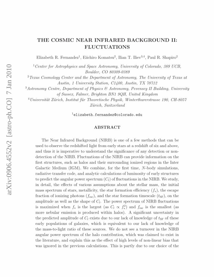
Fig. 4.— Non-linear bias of the halo mass-density power spectrum. (This is not the

luminosity-density power spectrum; see § 4.1 for the precise definition.) Top left panel:

The power spectra of the halo mass density, P haloM (k) are shown as the solid lines (z = 6 to

10 from top to bottom), the linear matter power spectra times the mean halo mass density

squared, Plin(k)(ρhaloM )2, are the dashed lines, and the shot noise power spectra, P shot

M , are

the dotted lines. Top right panel: We show the bias,√

[P haloM (k)− P shot

M (k)]/[(ρhaloM )2Plin(k)],

(z = 10 to 6 from top to bottom). The bias increases significantly as we go to smaller scales,

and this effect has been ignored in the previous calculations of the power spectrum of NIRB

fluctuations. Note that the minimum halo mass resolved in the simulation is 2.2× 109 M⊙.

The degree of non-linear bias would be smaller for a smaller minimum mass (see, e.g., Fig-

ure 6 of Trac & Cen 2007). Bottom left panel: The linear power spectrum, k3Plin(k)/(2π2).

Bottom right panel: Same as top right panel, but on a log-log axis.

– 19 –

Fig. 5.— δc/σ(MMin, z) versus redshift. The halos resolved in our simulation, with M >

Mmin = 2.2× 109 M⊙, are located on rare peaks (δc/σ(Mmin, z) & 2.5) at z & 7.

expected from the halo model (Cooray & Sheth 2002). These halos are very rare, located on

high peaks with δc/σ(Mmin, z) & 2.5 (see Figure 5).

This motivates our writing P haloL (k) as

P haloL (k) =

(ρhaloM Lh

Mh

)2

b2eff(k)Plin(k), (32)

where the pre-factor, ρhaloM Lh/Mh, is the mean halo luminosity density. In the left panel of

Figure 6 we show ρhaloM Lh/Mh (in units of nW Mpc−3) as a function of redshifts. We find

that the redshift evolution of ρhaloM Lh/Mh is very rapid; thus, the redshift evolution of the

halo luminosity density power spectrum, P haloL (k), is dominated by that of the mean halo

luminosity density.

What determines the evolution of the mean halo luminosity density? The answer is

– 20 –

Fig. 6.— (Left) Mean halo luminosity density computed from our simulation,

ρhaloM (z)Lh(z)/Mh, where lαν (z) is from equation (6), in units of nW Mpc−3 as a function

of redshifts, for various stellar populations given in Table 1. The waves in the lines where

fesc are higher are from the discrete redshift sampling of the Lyman-α line. We averaged

the luminosity over a rectangular bandpass of 1 − 2 µm. (Right) Halo mass collapse frac-

tion, ρhaloM (z)/(Ωmρc0), as a function of redshifts. The redshift evolution of ρhaloM Lh/Mh is

essentially determined by that of ρhaloM .

simple: it is determined by the rate at which the mass in the universe collapses into halos.

To show this, in the right panel of Figure 6 we show the halo mass collapse fraction, or

the ratio of ρhaloM to the mean comoving mass density of the universe, Ωmρc0, where ρc0 =

2.775× 1011 h2 M⊙ Mpc−3 is the critical density of the universe at the present epoch. The

evolution of the collapse fraction is fast, explaining the fast evolution of the mean halo

luminosity density.

As halos are discrete objects, and we do not expect to resolve individual halos con-

tributing to the diffuse NIRB, the observed NIRB power spectrum is a sum of the clustering

component and the shot noise component. If the shot noise dominates over the clustering

component, it would be very difficult to ascertain information on the structure from the sig-

nal of the NIRB. The shot noise component can be estimated by integrating the luminosity

squared over the mass function:

P shotL =

(Lh

Mh

)2

P shotM =

(Lh

Mh

)2 ∫dMh M2

h

dnh

dMh, (33)

where we have again assumed that each halo has a constant mass-to-light ratio, i.e., Lh/Mh

is independent of Mh.

– 21 –

4.2. IGM Contribution

For the IGM contribution, we have

δρIGML (x) =

(pIGM

n2HX

2e

)[Ccell(x)n

2cell(x)X

2e,cell(x)− (Ccelln

2cellX

2e,cell)

], (34)

where pIGM is the volume emissivity of the IGM, integrated over the observed frequencies,

i.e., pIGM ≡∫ ν2(1+z)

ν1(1+z)dνpIGM(ν), Ccell, ncell, Xe,cell are the clumping factor, the comoving

number density of hydrogen atoms, and the ionization fraction within a cell, respectively.

We compute ncell using

ncell =Ωb

Ωm

ρM,cell

µmp

, (35)

where µ = 0.59 and mp are the mean molecular weight of ionized gas and the proton mass,

respectively. We have used the mass density of N -body particles per cell, ρM,cell, multiplied

by the baryon fraction, Ωb/Ωm, for computing the mass density of baryons per cell, as we

have assumed that gas traces dark matter particles, i.e., N -body particles. The clumping

factor, Ccell ≡ n2actual/n

2cell, relates the actual density squared to the square of the density

averaged within a cell. In other words, Ccell captures the sub-grid clumping that is not

resolved by the simulation.

Following Iliev et al. (2007), we make a simplifying assumption that Ccell takes on

the same value everywhere in the simulation, and evolves with redshift z as Ccell(z) =

26.2917e−0.1822z+0.003505z2 ; thus, we have

δρIGML (x) = 26.2917e−0.1822z+0.003505z2

(pIGM

n2HX

2e

)[n2cell(x)X

2e,cell(x)− (n2

cellX2e,cell)

]. (36)

Note that pIGM/(n2HX

2e ) does not depend on x, and is given by Eq. (23) integrated over a

rectangular bandpass of 1− 2 µm in the observer’s frame.

5. RESULTS

5.1. Luminosity-density Power Spectrum

In Figures 7 and 8 we show the luminosity-density power spectra, PL(k), for halos and

their associated HII regions in the IGM for two of our populations: Population II stars with

a Salpeter initial mass spectrum with fesc = 0.19 and f∗ = 0.5 (Figure 7) and Population III

stars with a Larson initial mass spectrum with fesc = 1 and f∗ = 0.01 (Figure 8), assuming

a rectangular bandpass from 1− 2 µm.

– 22 –

Fig. 7.— (Left) Luminosity-density power spectrum of halos with Pop II stars obeying a

Salpeter initial mass spectrum, fesc = 0.19, and f∗ = 0.5, assuming a rectangular bandpass

from 1 − 2 µm. The shot noise for the halo contribution is also shown as the dotted lines.

(Right) Luminosity-density power spectrum of the IGM. The ionization fraction of the IGM

reaches 0.5 at about z ∼ 8.3. On large scales where the shot noise is sub-dominant, we find

PL(k) ∝ k−3/2, which yields Cl ∝ l−3/2 or l2Cl ∝ l1/2 (see § 5.2).

Fig. 8.— (Left) The same as the left panel of Figure 7 with Pop III stars with the Larson

initial mass spectrum, fesc = 1, and f∗ = 0.01. (Right) The same as the right panel of Figure

7 for comparison.

– 23 –

The luminosity-density power spectra of halos are approximately power-laws over the

entire range of wavenumbers that the simulation covers. At the highest redshift bin, z ∼ 16,

the power spectrum is entirely dominated by the shot noise at all scales. The lower the

redshifts are, the more power in excess of the shot noise we observe on large scales (because

the shot noise is most important on small scales). The growth of the power spectrum is

partly driven by the growth of linear matter fluctuations as well as that of halo bias, i.e.,

the clustering of halos is biased relative to the underlying matter distribution. As we have

shown in the previous section, the bias of halos that we observe in the simulation is highly

non-linear, and thus has an important implication for the predicted shape of the observed

power spectrum of NIRB fluctuations. However, as we have shown in § 4.1, the evolution

of PL(k) is almost entirely driven by the fast growth of the mean halo luminosity density,

ρhaloM (z)Lh(z)/Mh (see Eq. (32) and the left panel of Figure 6). As a result PL(k) grows by

about six orders of magnitude at k = 0.1 Mpc−1 from z ∼ 13 to z ∼ 6, which is much faster

than the growth expected from the growth of bias times the matter power spectrum.

The luminosity-density power spectrum of the IGM increases quickly as the mean ioniza-

tion fraction, Xe, approaches 0.5 (at about z ∼ 8.3 for this particular simulation), especially

on larger scales. As the ionization fraction increases, the luminosity of the HII region would

also increase (because luminosity is proportional to X2e ). Moreover, since we are looking

at the over-luminosity-density power spectrum of the IGM, the greatest power results when

there is the greatest difference between luminous regions and the average luminosity of the

IGM; thus, the power spectrum of X2en

2 grows rapidly as Xe approaches 1/2. However, this

rapid growth of the power stops when the entire IGM is ionized (Xe = 1), in which case the

over-luminosity-density power spectrum of the IGM is simply proportional to n2.

The most interesting feature of the luminosity-density power spectrum of the IGM is a

“knee” feature, which is at k ∼ 2 Mpc−1 at z ∼ 16, and moves to k . 1 Mpc−1 at z . 10.

This “knee” is caused by the typical size of HII bubbles: the knee wavenumber is inversely

proportional to the typical size of the bubbles. At the highest redshift bin, z ∼ 16, the

bubbles are nearly Poisson-distributed, and thus the power spectrum is flat up to the knee

scale, k ∼ 2 Mpc−1, beyond which the power decreases as one is looking at the scales inside

the bubbles, which are smooth. As the redshift decreases, the knee scale moves to larger

scales, signifying a growth in the ionized bubbles with time until they merge. At the same

time, the large-scale power also grows, and the shape of the HII region power spectrum is

basically the same as that of the halo power spectrum, as the bubbles are created around

the halos.

Note that Iliev et al. (2006, 2007) studied the power spectrum of ionized gas density,

and observed a similar trend. The power spectrum of the luminosity density that we have

– 24 –

presented here is the four-point function of the ionized gas density (as the volume emissivity

is proportional to the ionized gas density squared), and thus it is different from the power

spectrum of the ionized gas density (which is quadratic in density).

5.2. Angular Power Spectrum of NIRB Fluctuations

What about the observable, the angular power spectrum of NIRB fluctuations, Cl?

We compute the angular power spectrum of NIRB fluctuations, Cl, by projecting PL(k) on

the sky. We do this using Limber’s approximation, and obtain (see Appendix A for the

derivation)

Cl =c

(4π)2

∫dz

H(z)r2(z)(1 + z)4PL

(k =

l

r(z), z

), (37)

where r(z) = c∫ z

0dz′/H(z′) is the comoving distance. We integrate Eq. (37) over the range

of redshifts that the simulation covers for both halos and the IGM, z = 6.0− 15.7.

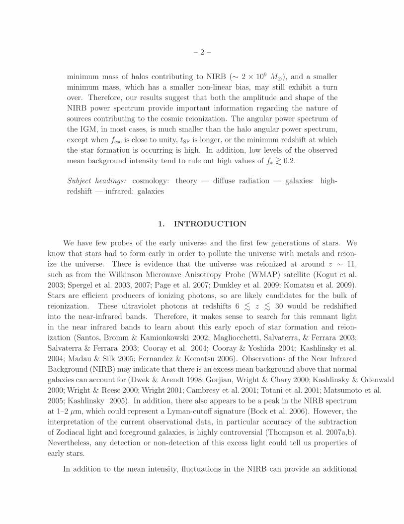
In Figure 9 we show l(l + 1)Cl/(2π) for halos with Population II stars with a Salpeter

mass spectrum and f∗ = 0.5 (the angular power spectrum for halos with the highest ampli-

tude) and for Population III stars with a Larson mass spectrum and f∗ = 0.01 (the angular

power spectrum for halos with the lowest amplitude), along with the angular power spec-

trum of the IGM. The halo contribution at small scales, i.e., l & 104, is comparable to the

shot noise contribution. When the shot noise is subtracted (see Figure 10), we find that

l(l + 1)Cl/(2π) is nearly a power-law, l(l + 1)Cl/(2π) ∝ l0.5, with no sign of a turn-over,

which would be expected from the shape of the projected linear matter power spectrum. This

is in a stark contrast with the previous calculations (Kashlinsky et al. 2004; Cooray et al.

2004), which predicted a turn-over at l ∼ 103. They assumed that the luminosity-density

power spectrum was given by the linear bias model, in which the halo power spectrum is a

constant times the matter power spectrum. Our calculations, which are based on a realistic

simulation, indicate that the simple linear bias model is not valid for these populations. This

is expected, as these populations are very highly biased, and therefore non-linear bias must

also be large, as demonstrated already in Figure 4.

On the other hand, there is no freedom in changing the amplitude of the IGM power

spectrum for a given simulation, i.e., a given fγ/tSF; thus, we show only one line for the

IGM contribution in Figure 9 (the lowest line). For the parameter space explored here,

the halo contribution can be as low as being only slightly over an order of magnitude (for

PopIII Larson with fesc = 1 and f∗ = 0.01) to about 106 times greater (for PopII Salpeter

with fesc = 0.19 and f∗ = 0.5) than the IGM contribution. If we were to increase fγ(which is possible using additional simulations in future work, although one has to make

– 25 –

Fig. 9.— Angular power spectra of NIRB fluctuations, Cl, from halos in comparison to the

angular power spectrum of the IGM (the bottom line). We show Cl from halos that have

Population II stars with a Salpeter mass spectrum and f∗ = 0.5 (the angular power spectrum

that has the highest amplitude) and Population III stars with a Larson mass function and

f∗ = 0.01 (the angular power spectrum with the lowest amplitude and which is closest to the

angular power spectrum of the IGM). The dotted lines show the level of the shot noise. In

Figure 11 we show how the amplitude of the power spectrum changes between populations

with various escape fractions of the ionizing photons into the IGM, fesc, and star formation

efficiencies, f∗. (Right panel) Same as the left panel, except divided by f 2∗. The IGM

contribution is not shown.

– 26 –

Fig. 10.— The angular power spectrum from the clustering of halos (solid line), i.e., the

angular power spectrum minus the shot noise contribution. The dotted line has a slope of

l0.5. The clustered angular power spectrum shows no evidence of a turnover that was claimed

to exist in the literature. This is because previous analytical models in the literature based

their power spectrum on the linear bias model, which is not valid for this population, which

has a high level of non-linear bias. The minimum halo mass used in this calculation is

2.2× 109 M⊙.

– 27 –

Fig. 11.— (Left panel) The change of the angular power spectrum as a function of the escape

fraction, fesc, for our selected samples of stellar populations. Each amplitude is scaled with

relation to the angular power spectrum of Population II stars with a Salpeter mass spectrum

and f∗ = 0.5. (Since the shape of the angular power spectra are the same for all stellar

populations, this ratio is the same for all wave numbers.) (Right panel) The dependence of

the angular power spectrum on f∗. The solid line shows Cl ∝ f 2∗. Note that each stellar

population has a different set of f∗, fesc, and Ni, and thus both panels show a slice of the

multi-parameter space.

sure that the resulting electron-scattering optical depth is consistent with the WMAP data),

a wider range of parameters fesc, f∗ and Ni could result. This is a good news, as this gives

us an opportunity to study the physics of the reionization using the power spectrum of

NIRB fluctuations. Sensitive surveys may be able to detect a change in the shape of the

power spectra that would be a result of the IGM power spectrum. This may be one way of

constraining fesc observationally.

In Figure 11, we show the amplitude of the angular power spectra of other stellar

populations scaled to the angular power spectrum of Population II stars with a Salpeter

mass spectrum and f∗ = 0.5. As we find in Eq. (9), the luminosity-density power spectrum

of halos is about proportional to f 2∗, and one of the terms in the power spectrum (nebular

contribution; the second term in Eq. (9)) depends on (1 − fesc). Therefore, for a fixed

fγ = fescf∗Ni and fixed Ni (i.e., fixed stellar population), the angular power spectrum of

the halo contribution must always increase as we increase f∗, as increasing f∗ must be

accompanied by the corresponding reduction in fesc, both of which will increase the power

spectrum of the halo contribution.

As Cl ∝ f 2∗, the parameter combinations that maximize f∗ tend to give the largest

Cl. For a fixed fγ = fescf∗Ni this means a lower Ni, i.e., lighter mass spectra with larger

– 28 –

metallicity (see the 5th column of Table 1), and a lower fesc. In reality, however, we should

also take into account the fact that heavier mass spectra produce more luminosity per stellar

mass, i.e., more l in Eq. (9). These factors explain the dependence of the predicted amplitudes

of l(l+1)Cl/(2π) (averaged over λ = 1−2 µm) on parameters shown in Figure 11. Populations

with higher fesc have lower angular power spectrum. This is to be expected, because as fescincreases, less photons are available to create luminosity within the halo.

6. VARYING THE MODEL: HALO CONTRIBUTION

In this section, we will focus on the halo contribution to the angular power spectrum of

NIRB fluctuations, and explore the effects of changing various parameters.

6.1. THE EFFECT OF THE STAR FORMATION TIMESCALE

As mentioned in section 3.1, the star formation timescale will affect the amplitude of

the angular power spectrum. We have assumed in this work a constant star formation

timescale of tSF = 20 Myr to make a consistent comparison between the halo and the IGM

contributions. However, the amplitude of Cl from halos depends sensitively on this rather

uncertain timescale, as the luminosity of halos is proportional to t−1SF , and thus Cl ∝ 1/t2SF.

Motivated by this, in this section we consider two other possibilities: 1) The star formation

time scale is shorter than the lifetime of the stars, in which case we will use equation 7 to

compute the luminosity per mass, and 2) the star formation is triggered by mergers, i.e.,

t−1SF(z) =

∫dMhMh(d

2nh/dMhdt)∫dMhMh(dnh/dMh)

, (38)

where dnh/dMh is the mass function of dark matter halos. For the Press-Schechter mass

function, we can calculate tSF(z) analytically from

t−1SF = H(z)

∣∣∣∣d lnD

d ln(1 + z)

∣∣∣∣[

δ2cD2(z)σ2(Mmin)

− 1

]≈ H(z)Ω0.55

m (z)

[δ2c

D2(z)σ2(Mmin)− 1

],

(39)

where δc = 1.68, D(z) is the growth factor of linear matter density fluctuations normalized

such that D(0) = 1, σ(Mmin) is the present-day r.m.s. matter density fluctuation smoothed

over a top-hat filter that corresponds to the minimum mass Mmin, and Ωm(z) is the matter

density parameter at a given z. Note that interpreting this quantity as a merger timescale

makes sense only when we study the density peaks above the r.m.s., i.e., δc/[D(z)σ(Mmin)] >

1. (Otherwise tSF becomes negative.) This formula has a clear physical interpretation: for

– 29 –

a density peak of order the r.m.s. mass density fluctuation, δc/[D(z)σ(Mmin)] − 1 ≈ 1, the

merger timescale is of order the Hubble time, i.e., tSF ≈ H−1(z). The higher the peaks are,

the shorter the merger timescale becomes; thus, in this model, high-z objects (for a given

mass) have shorter star formation timescales, and are brighter.

As the reionization history depends on fγ/tSF, changing only tSF without the corre-

sponding change in fγ results in a different reionization history. For example, increasing tSFby a factor of 10 makes individual sources fainter by a factor of 10, and thus it would result

in a much slower reionization history. To compensate this one would have to increase fγby a factor of 10. Moreover, if we reduce tSF by a large factor, it would make individual

sources brighter by a large factor, to the point where we might start detecting these sources

individually, e.g., as Lyman-α emitters (Fernandez & Komatsu 2008).

In this section, however, we explore the effects of tSF for a given fγ, to show how

important this quantity is for predicting the amplitude of NIRB fluctuations without any

extra information on reionization from WMAP or Lyman-α emitters.

The angular power spectrum for various assumptions for the star formation timescale

is given in Figure 12. The angular power spectrum with the highest amplitude corresponds

to when the star formation time scale is shorter than the lifetime of the stars. If the star

formation timescale is given by the merger time of halos (Eq. 39), the star formation timescale

varies with redshift and we obtain the lowest amplitude for the angular power spectrum, as

the merger timescale at a given redshift is usually comparable to the age of the Universe at

the same redshift. Our assumption of tSF = 20 Myr lies between these two extremes.

We can further quantify the uncertainty in Cl from tSF by looking at the mass-to-light

ratio of the galaxies (see Figure 13). We know very little about the nature of high-z galaxies

contributing to NIRB. We don’t know what the mass-to-light ratio is for these populations.

An uncertainty of a factor of 100 in the star formation timescale will correspond directly to

an uncertainty in the mass-to-light ratio of 100, and an uncertainty of 104 in the angular

power spectrum. Early galaxies could be starbursts, with a mass-to-light ratio of less than

0.1 to 1, or normal galaxies, with a mass-to-light ratio of & 10. The amplitude of Cl is,

among other things, a sensitive probe of the nature of high-z galaxies.

6.2. THE EFFECT OF CHANGING zend

The angular power spectra will also depend on what we choose for the end of the star

formation epoch, zend. The effect of our choice of zbegin is minimal, because at high redshift,

the halos are smaller and dimmer, contributing less to the angular power spectrum. (See

– 30 –

Fig. 12.— The effect of the star formation time scale on the angular power spectrum. We

find the largest amplitudes when tSF is shorter than the main sequence lifetime of stars,

whereas we find the lowest amplitudes when tSF is given by the timescale of halo mergers

(Eq. 39). The uncertainty due to the star formation time scale is large and can lead to an

uncertainty in the angular power spectrum of a factor of ≈ 104. This reflects our uncertainty

in the mass to light ratio of galaxies that contribute to the NIRB. However, note that not

all scenarios shown here yield the reionization histories that are consistent with the WMAP

data and the abundance of Lyman-α emitters. (Right panel) Same as the left panel, except

divided by f 2∗.

Fig. 13.— The bolometric mass-to-light ratio for halos for various star formation timescales.

Uncertainty in the amplitude of the star formation time scale can be equated to the un-

certainty in the mass-to-light ratio, i.e., the nature of high-z galaxies contributing to the

NIRB. The upper and lower sets of lines show the PopIII Larson and the PopII Salpeter,

respectively. (Right panel) Same as the left panel, except multiplied by f∗.

– 31 –

Figures 7 and 8.) Since halos and IGM will contribute more to fluctuations at lower redshifts,

we find that the angular power spectrum dramatically drop as we stop star formation at

higher redshifts (see Figure 14).

The shape of the angular power spectrum also changes as we vary zend. As zend increases,

the angular power spectrum of the halos steepens. The shape of the angular power spectrum

from the IGM can also affect the overall slope of the observed angular power spectrum if the

halo contribution is close to that of the IGM contribution. If the escape fraction is small,

this effect in the change of shape from the IGM will be less than if the escape fraction is

large. When zend is very large, the amplitude of the angular power spectrum of the IGM

could even be higher than that of the halos.

6.3. LYMAN-α ATTENUATION

The Lyman-α line can be attenuated by dust or neutral hydrogen. To understand this

effect one would have to perform detailed calculations of the radiation transport of Lyman-α

photons, including scattering of Lyman-α photons; however, such calculations are usually

quite complex and time-consuming. Therefore, in this subsection we study the extreme

limit of attenuation: the case where all of the Lyman-α photons are absorbed or extinct.

How would this affect the angular power spectrum? The effect of the complete Lyman-α

attenuation is shown in Table 2. The effect of the Lyman-α attenuation is the greatest when

the Lyman-α line is the strongest (for heavy Pop III stars) and when the escape fraction

is smaller (so more photons stay within the halo to produce nebular emission). The effect

of Lyman-α attenuation in the IGM is the highest, because normally a higher fraction of

emission is coming from the Lyman-α line (in the halos, there is also stellar emission).

7. COMPARISON TO PREVIOUS WORK

Cooray et al. (2004) made fully analytic predictions of the angular power spectrum

in the NIRB luminosity expected from the first stars in halos. They ignored the IGM

contribution, which we found to be small relative to the halo contribution for a range of

parameters we have explored in this paper. They modeled halos with 300 solar mass stars

for two cases: (1) an optimistic scenario - star formation in halos above 105 K, halos forming

stars from z = 10 − 30, and a star formation efficiency of 100%; and (2) a pessimistic

scenario - star formation beginning at 5000 K (so the bias is lower), halos forming stars from

z = 15−30, and a star formation efficiency of 10%. Using the same stellar masses (300 M⊙),

– 32 –

Fig. 14.— The angular power spectrum for halos and IGM as zend is varied. We show

the angular power spectrum for the halos with the highest and lowest amplitude of the

angular power spectrum (Population II stars with a Salpeter mass spectrum and f∗ = 0.5

and Population III stars with a Larson mass spectrum and f∗ = 0.01 respectively) and the

IGM. The angular power spectrum as shown throughout the rest of the paper has zend = 6.

As zend increases, the angular power spectrum drops. At very high redshifts, the angular

power spectrum of the IGM is higher than some of the angular power spectrum of the halos.

(Right panel) Same as the left panel, except divided by f 2∗. The IGM contribution is not

shown.

– 33 –

Population Initial Mass Spectrum fesc f∗ Cl, Lyα atten/Cl, no atten

Pop III Salpeter 0.22 0.2 0.848

Pop III Larson 0.1 0.1 0.632

Pop III Salpeter 0.9 0.05 0.975

Pop III Larson 1 0.01 1

Pop II Salpeter 0.95 0.1 0.995

Pop II Larson 0.9 0.023 0.974

Pop II Salpeter 0.19 0.5 0.926

Pop II Larson 0.098 0.21 0.825

IGM 0.448

Table 2: The effect of Lyman-α attenuation on the angular power spectrum. Here, we assume

complete attenuation (no production of Lyman-α photons). The angular power spectrum is

only slightly affected in most cases, and is more affected in cases where the Lyman-α line

was strong to begin with (such as heavy Pop III stars). The effect of Lyman-α attenuation

in the IGM is the highest, as the IGM does not have the stellar contribution, and is mainly

dominated by the Lyman-α and two-photon emission.

we have compared our results from the simulation to the optimistic case from Cooray et al.

(2004) for two different escape fractions, 0 and 1, and show the results in Figure 15 for

different wavelengths. As in Cooray et al. (2004), we use the star formation time scale given

by the merger time scale (see Eq. 38). The angular power spectrum here is

Cνν′

l =c

(4π)2

∫dz

H(z)r2(z)(1 + z)2Pp

(ν(1 + z), ν ′(1 + z); k =

l

r(z), z

), (40)

which gives the angular power spectrum at only one wavelength (rather than that averaged

over a certain bandpass). The difference between this equation and Eq. (37) is a factor of

(1 + z)2 since we are no longer integrating over a range of frequencies (see Appendix A for

the derivation). Note that we do not show Cl at 1 µm: at 1 µm, the emission comes from

photons that are more energetic than hν = 13.6 eV in the rest frame at z > 10. Because of

this, there should be no emission from the halos themselves, if one considers halos at z > 10.

(There would be contributions if one considered halos at lower redshifts, say, z > 6.)

Since there were not enough halos in our simulation to create an accurate power spec-

trum above z = 16.6, our population of stars only goes from 10 < z < 16.6, while the model

from Cooray et al. (2004) included star formation from 10 < z < 30. However, this should

not make too much of a difference, because halos at higher redshift do not contribute as much

to the angular power spectrum. In Figure 15 we show the angular power spectrum minus

– 34 –

Fig. 15.— Comparison to Cooray et al. (2004) (shown as triple-dot dashed lines). We show

l(l + 1)Cl/(2π) where Cl = ν2Cννl (see Eq. 40), from halos at z > 10 that host only very

massive stars with 300 M⊙, at various wavelengths. The total angular power spectra from

this work are shown as solid lines, shot noise is shown as dotted lines, and the clustered

angular power spectra, which are the total power minus the shot noise components, are

shown as dashed lines. Note that the amplitudes of Cl shown here are much smaller than

those shown in the previous figures (despite a high star formation efficiency, f∗ = 1), as we

have removed the most dominant, lower redshift contributions, z < 10, in this figure, to be

compatible with Cooray et al. (2004). See Figure 14 for the effects of changing the minimum

redshift of star formation. The mean intensity, νIν , for this population of stars at 2µm and

4µm are 63 and 16 nW m−2 sr−1 respectively, which is already ruled out by observations

(see section 9).

– 35 –

the shot noise, which will give us the angular power spectrum of the clustered component,

which is directly comparable to the quantity from Cooray et al. (2004). We have included

all the nebular processes including the free-bound and two-photon emission, which are im-

portant to the overall luminosity of the halo and which Cooray et al. (2004) have neglected.

The overall amplitude of our angular power spectrum is lower than that which Cooray et al.

(2004) predicted, by a large factor, 103. 4

In addition, the angular power spectrum from Cooray et al. (2004) peaks at about

l ∼ 1000 and then turns over. This is because Cooray et al. (2004) did not take into account

the nonlinear bias in the halo power spectrum. Nonlinear bias will increase the power at

small scales, especially at high redshifts, where galaxies were more highly biased. We again

refer to Figure 4, which shows the importance of non-linear bias. This greatly affects both

the amplitude and the shape of the angular power spectrum of the NIRB and should be

included.

8. OBSERVING THE FLUCTUATIONS IN THE NEAR INFRARED

BACKGROUND

Interpretation of the NIRB data can be a challenging task. Instrument emission, fore-

grounds and zodiacal light must all be taken into account. Foreground stars and low-redshift

galaxies, in addition to very faint and the dim wings of galaxies, must be removed. Much of

the differences in the existing measurements of the fluctuations from stars at high redshift

result from differences in how lower redshift galaxies are accounted for. Foreground galax-

ies are removed down to a limiting magnitude (which is usually different between different

observations). Galaxies fainter than this are taken into account using different methods.

There have been several observations of the NIRB. Kashlinsky & Odenwald (2000) found

fluctuations at the wavelengths from 1.25 to 4.9µm in the images taken by the Diffuse Infrared

Background Experiment (DIRBE) on Cosmic Background Explorer (COBE), which were not

consistent with the Galactic emission or instrument noise. Matsumoto et al. (2005) observed

the NIRB using the Infrared Telescope in Space (IRTS). They detected a clustering excess

on scales of about 100′ from 1.4 to 4 µm, and an indication of a spectral jump from the

high redshift Lyman cutoff. This jump could indicate that Population III star formation

4This difference may be explained by the fact that Cooray et al. (2004) actually rescaled the overall ampli-

tude to fit the mean intensity measured by the Infrared Telescope in Space (IRTS) (Matsumoto et al. 2005)

and the Diffuse Infrared Background Experiment (DIRBE) (Kashlinsky & Odenwald 2000). (A. Cooray,

private communication.)

– 36 –

ended at about a redshift of z ∼ 9. Excess fluctuations were detected, possibly from high

redshift galaxies, at about 1/4 of the mean intensity. Kashlinsky et al. (2007c, 2005) made

observations of the fluctuations of the NIRB using the Infrared Array Camera (IRAC) on

the Spitzer Space Telescope at 3.6, 4.5, 5.8 and 8 µm. Sources were removed by clipping

pixels containing & 4σ peaks, as well as removing fainter sources identified by SExtractor

and convolved with the appropriate point spread function of IRAC. Since zodiacal light is

not fixed in celestial coordinates, it was removed by taking observations six months apart in

fields rotated by 180. They detected excess fluctuations (0.1 nW m−2 sr−1 at 3.6 µm) that

were not consistent with instrument noise, dim wings of galaxies, zodiacal light, or galactic

cirrus. They claim that it is possible that the excess fluctuations came from high redshift

galaxies (z > 6.5) or faint, low redshift galaxies. However, since these fluctuations show

little (< 10−3) correlation with the ACS source catalog maps, and the power spectrum of

fluctuations is inconsistent with the Hubble Space Telescope Advanced Camera for Surveys

(ACS) catalog galaxies, they state it is unlikely that these fluctuations are from faint, low-z

galaxies (Kashlinsky et al. 2007a). However, Thompson et al. (2007b) claim that the color

of the fluctuations detected by Kashlinsky et al. (2007c, 2005) are consistent with objects at

z < 10, and therefore not from a population of high redshift stars.

Cooray et al. (2007) observed the NIRB using IRAC at 3.6 µm. They masked the image

to cut out faint, low redshift galaxies. In their most extensive masked image, they masked

IRAC sources down to a magnitude of 20.2 in addition to galaxies in ACS catalog. They

also discarded pixels that had a flux 4σ above the mean.

Thompson et al. (2007a) also made observations of the fluctuations of the NIRB using

the Near Infrared Camera and Multi-Object Spectrometer (NICMOS) camera on the Hubble

Space Telescope at 1.1 and 1.6 µm. The effects of zodiacal light were removed by dithering

the camera. After removing galaxies down to the fainter ACS and NICMOS detection limit,

fluctuation power dropped two orders of magnitude in comparison to an earlier paper by

Kashlinsky et al. (2002). Therefore, Thompson et al. (2007a) confirmed that the observed

fluctuations reported by Kashlinsky et al. (2002) in the 2MASS data are from low redshift

galaxies (z < 8) (although they are unable to rule out contributions from galaxies in 8 <

z < 13). Yet, they concluded that an excess fluctuation power in the NIRB of about

1 − 2 nW m−2 sr−1 could still be from the first stars. Their methodology would miss

fluctuations that are flat on scales above 100′′ or clumped on scales of a few arc minutes.

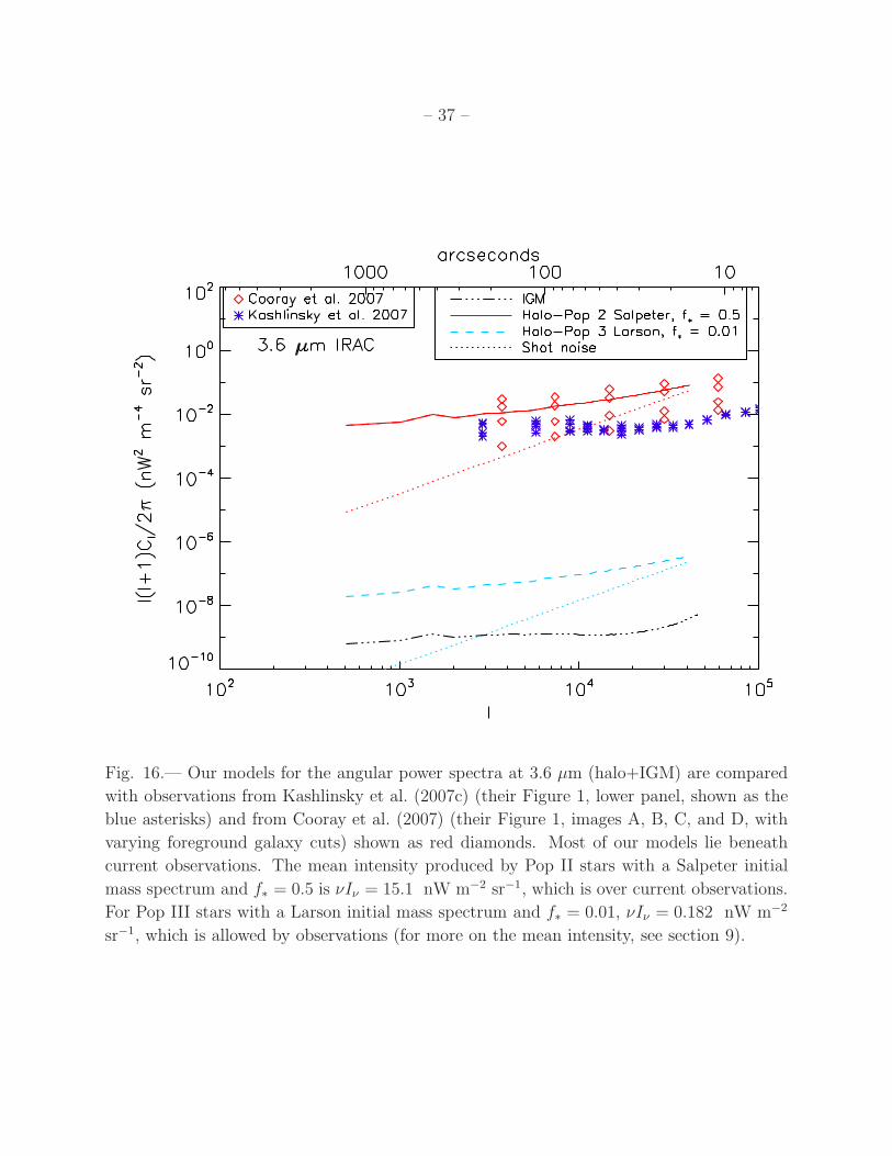
Our models are compared to the observations at 3.6 µm by Kashlinsky et al. (2007c,

2005) and Cooray et al. (2007) in Figures 16 and to observations at 1.6 µm from Thompson et al.

(2007a) in Figure 17. For these observations, it is safe to treat them as “upper limits,” as

additional foreground contamination might still exist. At 3.6 µm, most of our predictions for

– 37 –

Fig. 16.— Our models for the angular power spectra at 3.6 µm (halo+IGM) are compared

with observations from Kashlinsky et al. (2007c) (their Figure 1, lower panel, shown as the

blue asterisks) and from Cooray et al. (2007) (their Figure 1, images A, B, C, and D, with

varying foreground galaxy cuts) shown as red diamonds. Most of our models lie beneath

current observations. The mean intensity produced by Pop II stars with a Salpeter initial

mass spectrum and f∗ = 0.5 is νIν = 15.1 nW m−2 sr−1, which is over current observations.

For Pop III stars with a Larson initial mass spectrum and f∗ = 0.01, νIν = 0.182 nW m−2

sr−1, which is allowed by observations (for more on the mean intensity, see section 9).

– 38 –

Fig. 17.— Our models for the angular power spectra (halo+IGM) are compared with obser-

vations from Thompson et al. (2007a) (for all sources deleted) at 1.6 µm, which are shown

by the blue diamonds. Again, most of our models lie beneath current observations. As in the

case at 3.6µm, the mean intensity from Pop II stars with a Salpeter initial mass spectrum

and f∗ = 0.5 is high at νIν = 60.1 nW m−2 sr−1, while the mean intensity for Pop III stars

with a Larson initial mass spectrum and f∗ = 0.01 is νIν = 0.802 nW m−2 sr−1.

– 39 –

Fig. 18.— Our models of the angular power spectrum (halos and the IGM) compared

with the sensitivities of upcoming CIBER missions (shown as the stepped blue lines) from

Cooray et al. (2009). CIBER will increase sensitivity of measured fluctuations, but still

many of our models will lie beneath the detection limit.

the angular power spectra are below the current observations, and are therefore still viable

candidates. At 1.6 µm we see similar results. Therefore, it seems likely that early stars

contribute at very low levels to the fluctuations in NIRB. Of course, other factors, such as

the star formation time scale and the minimum redshift that star formation occurs at, zend,

can also affect which models can agree with observations.

Missions currently underway and future, more detailed experiments can make better ob-

servations of the NIRB. AKARI (previously known as ASTRO-F) observed in 13 bands from

2-160 µm (Matsuhara et al. 2008). The Cosmic Infrared Background Experiment (CIBER)

will be able to obtain the power spectrum from 7′′ to 2 degrees. Combined with AKARI

and Spitzer, fluctuations 100 times fainter than IRTS/DIRBE will be able to be observed.

CIBER has two dual wide field imagers at 0.9 and 1.6 µm. An improved CIBER II will also

measure fluctuations in four bands from 0.5 to 2.1 µm. This experiment will be pivotal to

determine if the fluctuations observed are from the first galaxies or have a more local origin

(Bock et al. 2006; Cooray et al. 2009). Predictions for the sensitivity of CIBER I and II are

shown in Figure 18 for both 0.9 and 1.6 µm (I and H-Band respectively) (Cooray et al. 2009;

Bock et al. 2006). The sensitivity of CIBER will be much better than any of the current

observations, but still many of our models lie beneath detection limits.

– 40 –

f∗ ρ∗(z = 6) ρ∗(z = 10) ρ∗(z = 15)

0.2 1.9 3.7× 10−2 1.0× 10−4

0.01 9.6× 10−2 1.9× 10−3 5.1× 10−6

0.001 9.6× 10−3 1.9× 10−4 5.1× 10−7

Table 3: Values of the star formation rate computed from our simulation, ρ∗, in units of

M⊙ yr−1 Mpc−3. We have used the star formation timescale of tSF = 20 Myr.

9. ADDITIONAL CONSTRAINTS FROM THE MEAN INTENSITY OF

THE NEAR INFRARED BACKGROUND

In addition to fluctuations, measurements have been taken of the mean intensity of the

NIRB. Because these measurements rely on an accurate subtraction of the zodiacal light,

measurements of the mean intensity of the NIRB are more difficult to perform. Currently,

the interpretation of these measurements is still highly controversial. Measurements of the

excess in the NIRB (NIRBE) started out high (70 nW m−2 sr−1) (Matsumoto et al. 2005)

and have since declined. The most recent measurements are lower. Kashlinsky et al. (2007b)

report that the mean intensity of the NIRBE must be greater than 1 nW m−2 sr−1 to be

consistent with fluctuations at 3.6 and 4.5 µm. Thompson et al. (2007a) report a residual

NIRBE of 0.0+3−0.3 at 1.1 and 1.6 µm. Fluctuations measured by Cooray et al. (2007) imply

that the mean NIRB cannot be much more than 0.5 nW m−2 sr−1 at 3.6 µm. Using these

limits, can we put additional constrains on the first stars?

We calculate the mean intensity of NIRB from (Peacock 1999)

Iν =c

4π

∫dz p([1 + z]ν, z)

H(z)(1 + z), (41)

where ν is the observed frequency and p(ν, z) is given by Eq. (2). The star formation rate

contained in p(ν, z), is given by ρ∗(z) = ρ∗(z)/tSF(z), where

ρ∗(z) = f∗Ωb

ΩmρhaloM (z), (42)

where ρhaloM (z) is the mean mass density collapsed into halos taken from the simulation (which

has the minimum halo mass of 2.2 × 109 M⊙), and is shown in the right panel of Figure 6.

For the star formation timescale, we use tSF = 20 Myr, so that we can calculate the mean

NIRB for models that are compatible with the WMAP data. The star formation rates with

various star formation efficiencies are given in Table 3.

We can now calculate the mean intensity of NIRB for our models with various stellar

populations and values of f∗. The value of fesc does not matter here because when calculating

– 41 –

Fig. 19.— Spectra of the NIRBE from various populations of stars over a redshift range of

6 to 15. (Left panel) Changing initial mass spectrum and metallicity of the stars for a given

star formation efficiency, f∗ = 0.01. (Right panel) Changing the star formation efficiency for

Population III stars with a Salpeter initial mass spectrum. Models with high star formation

efficiency, f∗ = 0.2, produce too high NIRB, and can be ruled out by the current upper limits

from observations. Note that if we divided these curves by f∗, they would become identical.

In other words, these curves differ solely due to the varying values of f∗.

the mean intensity - it does not matter where the photons are coming from - the halo itself

or the IGM surrounding the halo (Fernandez & Komatsu 2006). The spectra of NIRB from

various populations of stars (with varying mass, metallicity, and f∗) over the redshift range

of z = 6 − 15 (using simulation data up to the redshift 14.6) are shown in Figure 19, and

their numerical values (integrated over 1 − 2 µm) are tabulated in Table 4. We also show

the spectra of each radiation process in Figure 20. Finally, we show the mean intensity from

two redshift bins, z = 6−10 and 10−15, in Figure 21. Lower redshift stars clearly dominate

over stars at higher redshifts. This, combined with a sharp break due to the Lyman limit as

well as a bump due to the Lyman-α line, may be used to constrain zend.

Assuming that our equation for the star formation rate is accurate up to high redshifts,

and using the parameters of this simulation, we can put constraints on the populations of first

stars. If we take our upper limit for the mean intensity of the NIRBE to be 3 nW m−2 sr−1

(the upper limit from Thompson et al. (2007a)), we can rule out most populations with

high star formation efficiencies (f∗ = 0.2), unless star formation is constrained to only high

redshifts. This is consistent with our fluctuation analysis - some of our models with high

f∗ would produce angular power spectra above the levels observed. If the star formation

efficiency is very low, say, f∗ = 0.001, then the mean background would be too small to

detect. Most of the change in the amplitude of the NIRBE is from a change in the star

formation efficiency f∗, while the metallicity and initial mass spectra of the stars affect the

– 42 –

Fig. 20.— Spectra of the NIRBE and how each component contributes to the overall inten-

sity, over a redshift range of 6 to 15.

shape of the spectra. Therefore, an accurate measurement of the mean NIRBE can give

information on the star formation efficiency. Further constraints on the metallicity and mass

may be possible with more precise observations in the future.

10. PREDICTIONS FOR FRACTIONAL ANISOTROPY

As we have seen, the magnitude of the predicted angular power spectrum depends on

various parameters such as f∗, tSF, fesc, and the initial mass spectrum. However, as the

mean intensity also depends on these quantities, one may hope that the ratio of the power

spectrum and the mean intensity squared would depend much less on these astrophysical

parameters.

– 43 –

f∗ Redshift Range νIνPop III Larson Pop III Salpeter Pop II Larson Pop II Salpeter

0.2 6− 15 32.2 22.9 43.2 32.2

0.01 1.61 1.15 2.16 1.61

0.001 0.161 0.115 0.216 0.161

Table 4: Values of the mean background intensity, νIν , in units of nW m−2 sr−1 for stars

with different star formation efficiencies. The mean is calculated as an average of νIν over 1

to 2 µm.

Ignoring the IGM contribution and rewriting the halo contribution given by equa-

tion (37), we get

Cl =c

(4π)2

(f∗

Ωb

Ωm

)2 ∫dz

H(z)r2(z)(1 + z)4

×[ρhaloM (z)

l∗(z) + (1− fesc)

[lff(z) + lfb(z) + l2γ(z) + lLyα(z)

]]2

×b2eff

(k =

l

r(z), z

)Plin

(k =

l

r(z), z

). (43)

By rewriting and averaging equation (41) over a band, we get

I =c

4π

(f∗

Ωb

Ωm

)∫dz

H(z)(1 + z)(44)

×ρhaloM (z)[l∗(z) + lff (z) + lfb(z) + l2γ(z) + lLyα(z)

]. (45)

Therefore, in the ratio Cl/I2, f∗ and tSF (which is related to lα as lα ∝ 1/tSF) cancel

out exactly. The dependence on the initial mass spectrum, f(m), which determines lα via

integral, nearly cancels out. However, the dependence on fesc does not cancel out: the power

spectrum depends on fesc, whereas the mean intensity does not. Therefore, we conclude that

the ratio depends primarily on fesc. In Figure 22 we show the fractional anisotropy, δI/I ≡√l(l + 1)Cl/(2πI2), for various infrared bands. Here, I is the mean intensity averaged over

the bands defined in Table 5, which are taken from Sterken & Manfroid (1992). We assume

a rectangular bandpass. The upper curves are for fesc = 0.19, while the lower curves are for

fesc = 1, which is consistent with the expectation: the ratio of the angular power spectrum

to the mean intensity is lower for a higher fesc. We have checked that the ratio is nearly

the same for different mass spectra for fesc = 0, in which case the dependence on l(z) nearly

cancels out.

Note that for fesc = 0 the ratio, Cl/I2, may be regarded as an weighted average of

b2eff (l/r)Plin(l/r). We find δI/I =√l(l + 1)Cl/(2πI2) ≈ 10−2 with a weak dependence on

– 44 –

Fig. 21.— Spectra of the NIRBE for populations of stars over two redshift bins, z = 6− 10

and 10− 15.

l, i.e., δI/I ∝ l0.25. In other words, the expected fractional anisotropy of the near infrared

background is of order a few percent for fesc = 0, and can be lower by a factor of a few for

fesc = 1.

11. DISCUSSION AND CONCLUSIONS

Any detection or non-detection of fluctuations in NIRB can give us information on stars

forming at high redshifts, stars that could have helped to reionize the universe. The escape

fraction of ionizing photons, the star formation efficiency, and the mass and metallicity of

the stars can affect the amplitude and shape of the angular power spectrum of fluctuations

in NIRB.

– 45 –

Band Center (microns) Waveband (microns)

J 1.25 1.1-1.4

H 1.65 1.5-1.8

K 2.2 2.0-2.4

L 3.5 3.0-4.0

M 4.8 4.6-5.0

Table 5: Band definitions used for infrared bands. These are given in Table 16.2 in

Sterken & Manfroid (1992).

We modeled the angular power spectrum from halos and the surrounding IGM by com-

bining the analytic formulas for the luminosity of halos and the IGM with N -body simula-

tions coupled with radiative transfer for several different populations of stars. Shot noise is a

major contributor to the angular power spectrum of halos at small scales, so it is important

to include larger scales in observations to minimize the component of shot noise.

The star formation efficiency has a significant effect on the amplitude of the angular

power spectrum, with the amplitude of the angular power spectrum being proportional to

f 2∗. For a fixed fγ/tSF = fescf∗Ni/tSF (i.e., for a given reionization history), a combination

of parameters that maximize the star formation efficiency, f∗, give the largest NIRB power

spectrum; thus, the stars that are less massive and have more metals (smaller Ni), and are in

halos with a lower escape fraction (smaller fesc) will all increase the amplitude of the NIRB

angular power spectrum. In general, the amplitude of the angular power spectrum of the

halos (and the mean NIRBE) is mostly dominated by f∗, while the angular power spectrum

of the IGM can probe the ionization history though the factor fγ/tSF .

If we do not fix the reionization history, there are other parameters that can change

the amplitude of the angular power spectrum significantly. The angular power spectrum is

inversely proportional to the star formation time scale squared, Cl ∝ 1/t2SF. This uncertainty

in the star formation time scale can be directly related to our uncertainty in the mass to light

ratio of galaxies, for tSF ∝ Mh/Lh. As changes in tSF result in different reionization histories

(for a given fγ), the other tracers of reionization, e.g., the electron-scattering optical depth

measured by the WMAP satellite and the abundance of Lyman-α emitting galaxies, should

help narrow down a range of magnitudes of the NIRB fluctuations that are consistent with

what we already know about the cosmic reionization.

The angular power spectrum of the IGM is typically a minor contributor to the overall

fluctuations; however, the IGM contribution can be comparable to the halo contribution (the

stellar contribution as well as the nebular contribution from within the halo), especially if

– 46 –

the escape fraction of ionizing photons from halos is high. In the limit that fesc is close to

unity, we expect CIGMl /Chalo

l ∝ f 2esc, as C

halol would be completely dominated by the stellar

emission. One can even make the IGM contribution dominate over the halo contribution by

increasing tSF, which suppresses the halo contribution as Chalol ∝ t−2

SF , and leads to a delay in

the reionization. Yet, this would not change the IGM power spectrum significantly, as the

IGM luminosity power spectrum saturates when the ionization fraction reaches Xe ∼ 0.5.

Of course, we need to make sure that such a model can still complete the reionization by

z ∼ 6, and can reproduce the electron-scattering optical depth measured by WMAP.

The redshift at which the formation of stars contributing to NIRB ends, zend, can also

change the amplitude of the angular power spectrum significantly. Changing zend affects not

only the amplitude of the angular power spectrum, but also the shape. The attenuation of

Lyman-α photons for the most part, does not affect the angular power spectrum of the halos

greatly, but could affect the amplitude of the IGM by about a factor of 2.

Previous estimates of the angular power spectrum of the NIRB by Cooray et al. (2004)

neglected to account for nonlinear bias. For our simulation with the minimum halo mass of

2.2×109 M⊙, the nonlinear bias is large enough to change the prediction for the shape of the

angular power spectrum qualitatively: a turnover of l(l+1)Cl at l ∼ 103 that was predicted by

Cooray et al. (2004) is not seen in our calculation, and the shape of the clustering component

(i.e., minus the shot noise), is consistent with a pure power law, l(l + 1)Cl ∝ l0.5.

Note that our results for the shape of the angular power spectrum are valid for the

minimum halo mass of Mmin = 2.2 × 109 M⊙. The non-linear bias would be smaller for

smaller mass halos. For example, the simulation carried out by Trac & Cen (2007) resolves

halos down to a smaller mass, Mmin = 6 × 107 h−1 M⊙, and would therefore find a smaller

average bias. The halo bias is mass dependent, more massive halos being more strongly

biased. The effective linear bias, beff,lin, is the integral of the linear halo bias for a given

mass, b1(Mh), times the mass function weighted by mass above a certain minimum mass,

i.e., beff,lin = [∫∞

MmindMh Mh(dnh/dMh)b1(Mh)]/[

∫∞

MmindMh Mh(dnh/dMh)]. As there are

many more halos at lower masses, lowering Mmin would result in a lower average bias. As

the degree of the non-linear bias increases as the linear bias increases, one would find a

smaller non-linear bias for a lower Mmin. Therefore, we might still see a turnover if these

smaller halos are bright enough to contribute to the NIRB.

However, the real situation would be more complex than the above picture. In Iliev et al.

(2007), we also performed reionization simulations which resolve source halos down to this

lower minimum mass of ∼ 108 M⊙. There, however, unlike Trac & Cen (2007), we took

account of the fact that those small-mass (. 109 M⊙) halos are subject to Jeans filtering,

and thus their star formation is suppressed if they reside within the ionized regions. The sup-

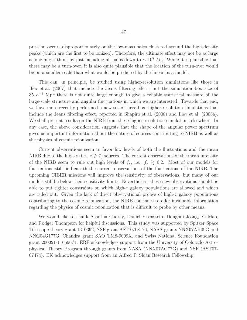
– 47 –

pression occurs disproportionately on the low-mass halos clustered around the high-density

peaks (which are the first to be ionized). Therefore, the ultimate effect may not be as large

as one might think by just including all halos down to ∼ 108 M⊙. While it is plausible that

there may be a turn-over, it is also quite plausible that the location of the turn-over would

be on a smaller scale than what would be predicted by the linear bias model.

This can, in principle, be studied using higher-resolution simulations like those in

Iliev et al. (2007) that include the Jeans filtering effect, but the simulation box size of

35 h−1 Mpc there is not quite large enough to give a reliable statistical measure of the

large-scale structure and angular fluctuations in which we are interested. Towards that end,

we have more recently performed a new set of large-box, higher-resolution simulations that

include the Jeans filtering effect, reported in Shapiro et al. (2008) and Iliev et al. (2008a).

We shall present results on the NIRB from these higher-resolution simulations elsewhere. In

any case, the above consideration suggests that the shape of the angular power spectrum

gives us important information about the nature of sources contributing to NIRB as well as

the physics of cosmic reionization.

Current observations seem to favor low levels of both the fluctuations and the mean

NIRB due to the high-z (i.e., z & 7) sources. The current observations of the mean intensity

of the NIRB seem to rule out high levels of f∗, i.e., f∗ & 0.2. Most of our models for

fluctuations still lie beneath the current observations of the fluctuations of the NIRB. The

upcoming CIBER missions will improve the sensitivity of observations, but many of our

models still lie below their sensitivity limits. Nevertheless, these new observations should be

able to put tighter constraints on which high-z galaxy populations are allowed and which

are ruled out. Given the lack of direct observational probes of high-z galaxy populations

contributing to the cosmic reionization, the NIRB continues to offer invaluable information

regarding the physics of cosmic reionization that is difficult to probe by other means.

We would like to thank Asantha Cooray, Daniel Eisenstein, Donghui Jeong, Yi Mao,

and Rodger Thompson for helpful discussions. This study was supported by Spitzer Space

Telescope theory grant 1310392, NSF grant AST 0708176, NASA grants NNX07AH09G and

NNG04G177G, Chandra grant SAO TM8-9009X, and Swiss National Science Foundation

grant 200021-116696/1. ERF acknowledges support from the University of Colorado Astro-

physical Theory Program through grants from NASA (NNX07AG77G) and NSF (AST07-

07474). EK acknowledges support from an Alfred P. Sloan Research Fellowship.

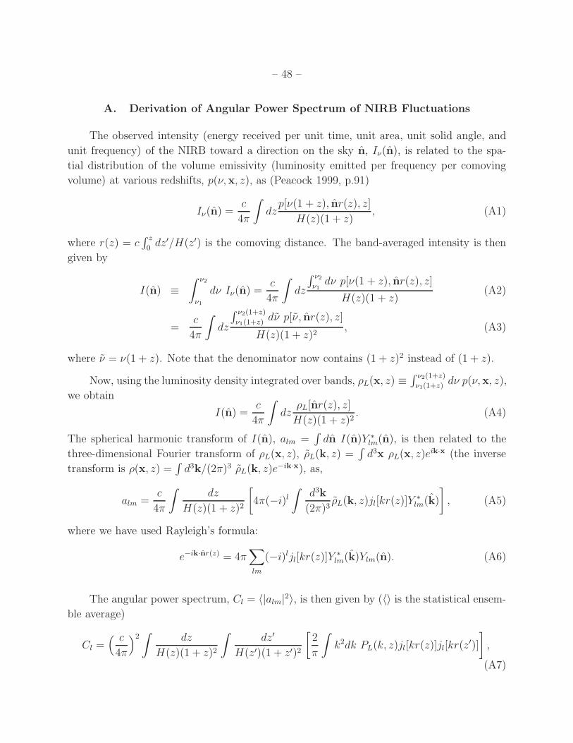
– 48 –

A. Derivation of Angular Power Spectrum of NIRB Fluctuations

The observed intensity (energy received per unit time, unit area, unit solid angle, and

unit frequency) of the NIRB toward a direction on the sky n, Iν(n), is related to the spa-

tial distribution of the volume emissivity (luminosity emitted per frequency per comoving

volume) at various redshifts, p(ν,x, z), as (Peacock 1999, p.91)

Iν(n) =c

4π

∫dz

p[ν(1 + z), nr(z), z]

H(z)(1 + z), (A1)

where r(z) = c∫ z

0dz′/H(z′) is the comoving distance. The band-averaged intensity is then

given by

I(n) ≡

∫ ν2

ν1

dν Iν(n) =c

4π

∫dz

∫ ν2ν1

dν p[ν(1 + z), nr(z), z]

H(z)(1 + z)(A2)

=c

4π

∫dz

∫ ν2(1+z)

ν1(1+z)dν p[ν, nr(z), z]

H(z)(1 + z)2, (A3)

where ν = ν(1 + z). Note that the denominator now contains (1 + z)2 instead of (1 + z).

Now, using the luminosity density integrated over bands, ρL(x, z) ≡∫ ν2(1+z)

ν1(1+z)dν p(ν,x, z),

we obtain

I(n) =c

4π

∫dz

ρL[nr(z), z]

H(z)(1 + z)2. (A4)

The spherical harmonic transform of I(n), alm =∫dn I(n)Y ∗

lm(n), is then related to the

three-dimensional Fourier transform of ρL(x, z), ρL(k, z) =∫d3x ρL(x, z)e

ik·x (the inverse

transform is ρ(x, z) =∫d3k/(2π)3 ρL(k, z)e

−ik·x), as,

alm =c

4π

∫dz

H(z)(1 + z)2

[4π(−i)l

∫d3k

(2π)3ρL(k, z)jl[kr(z)]Y

∗

lm(k)

], (A5)

where we have used Rayleigh’s formula:

e−ik·nr(z) = 4π∑

lm

(−i)ljl[kr(z)]Y∗

lm(k)Ylm(n). (A6)

The angular power spectrum, Cl = 〈|alm|2〉, is then given by (〈〉 is the statistical ensem-

ble average)

Cl =( c

4π

)2∫

dz

H(z)(1 + z)2

∫dz′

H(z′)(1 + z′)2

[2

π

∫k2dk PL(k, z)jl[kr(z)]jl[kr(z

′)]

],

(A7)

– 49 –

where we have used the definition of the luminosity-density power spectrum (Eq. (24)), and

the normalization of the spherical harmonics,∫dkYlm(k)Y

∗

lm(k) = 1.

Now, when l ≫ 1, the integral within the square bracket can be approximated as5

2

π

∫k2dk PL(k, z)jl[kr(z)]jl[kr(z

′)] ≈δ [r(z)− r(z′)]

r2(z)PL

(k =

l

r(z), z

). (A8)

Therefore,

Cl ≈( c

4π

)2∫

dz

H(z)(1 + z)2

∫dr′

dz′/dr′

H(z′)(1 + z′)2δ(r − r′)

r2(z)PL

(k =

l

r(z), z

)

=c

(4π)2

∫dz

H(z)r2(z)(1 + z)4PL

(k =

l

r(z), z

), (A9)

where r = r(z) and r′ = r(z′), and we have used dz/dr = H(z)/c. This is Eq. (37).

On the other hand, if one chooses to calculate Cl from a pair of Iν(n) and Iν′(n) instead

of a pair of the band-averaged intensities I(n), then (1+ z)4 in the denominator of Eq. (A9)

becomes (1 + z)2:

Cνν′

l =c

(4π)2

∫dz

H(z)r2(z)(1 + z)2Pp

(ν(1 + z), ν ′(1 + z); k =

l

r(z), z

), (A10)

where Pp(ν, ν′; k, z) is the power spectrum of the volume emissivity, p(ν, z). Eq. (A10) agrees

with Eq. (10) of Cooray et al. (2004). Note that their jν is p(ν)/(4π) in our notation, which

explains the absence of 1/(4π)2 in their Eq. (10). However, this result does not agree with

Eq. (3) of Kashlinsky et al. (2004), which originates from Eq. (11) of Kashlinsky & Odenwald

(2000). (See also Eq. (14) of Kashlinsky (2005).) Kashlinsky et al.’s formula has (1 + z)

in the denominator of Eq. (A10) instead of (1 + z)2, and thus it misses one factor of 1/(1 +

z). We were unable to trace the cause of this discrepancy. It is therefore possible that

Kashlinsky et al. (2004) over-estimated Cl by a factor of ∼ 10. As they have not taken into

account a short lifetime of massive stars in their calculations (i.e., they used Eq. (7) instead

of Eq. (6)), which yields another factor of ∼ 100 in Cl, it is possible that they over-estimated

Cl by a factor of ∼ 103.

5The exact integral of a product of two spherical Bessel functions is given by 2

π

∫k2dk jl(kr)jl(kr

′) =

δ(r − r′)/r2. When a function, F (k), is a slowly-varying function of k compared to jl(kr)jl(kr′), which is a

highly oscillating function for l ≫ 1, we may obtain 2

π

∫k2dk F (k)jl(kr)jl(kr

′) ≈ F (k = l/r)δ(r − r′)/r2.

This is the so-called Limber’s approximation.

– 50 –

REFERENCES

Ahn, K., & Shapiro, P. R. 2007, MNRAS, 375, 881

Ahn, K., Shapiro, P. R., Iliev, I. T., Mellema, G., & Pen, U.-L. 2009, ApJ, 695, 1430

Bock, J., et al. 2006, New Astron, 50, 215

Cambresy, L., Reach, W. T., Beichman, C. A., & Jarrett, T. H. 2001, ApJ, 555, 563

Chary, R., Cooray, A., & Sullivan, I. 2008, ApJ, 681, 53

Cooray, A., & Sheth, R. 2002, Phys. Rep, 372, 1

Cooray, A., & Yoshida, N. 2004, MNRAS, 351, L71

Cooray, A., et al. 2004, ApJ, 606, 611

Cooray, A., et al. 2007, ApJ, 659, L91

Cooray, A., et al. 2009, arXiv:0904.2016

Dunkley, J., et al. 2009, ApJS, 180, 306

Dwek, E., & Arendt, R. G. 1998, ApJ, 508, L9

Fernandez, E. R., & Komatsu, E. 2006, ApJ, 646, 703

Fernandez, E. R., & Komatsu, E. 2008, MNRAS, 384, 1363

Ferrara, A. 1998, ApJ, 499, 17

Gorjian, V., Wright, E. L., & Chary, R. R. 2000, ApJ, 536, 550

Haiman, Z., Abel T., & Rees M. J. 2000, ApJ, 534, 11

Haiman, Z., Rees M. J., & Loeb A. 1997, ApJ, 476, 458

Iliev, I. T., Mellema, G., Merz, H., Shapiro, P. R., & Pen, U.-L. 2008a, in TeraGrid08, in

press (arXiv:0806.2887)

Iliev, I. T., Mellema, G., Pen, U.-L., Merz, H., Shapiro, P. R., & Alvarez, M. A. 2006,

MNRAS, 369, 1625

Iliev, I. T., Mellema, G., Pen, U.-L., Bond, J. R., & Shapiro, P. R., 2008b, MNRAS, 384,

863

– 51 –

Iliev, I. T., Mellema, G., Shapiro, P. R., & Pen, U.-L. 2007, MNRAS, 376,534

Jeong, D., & Komatsu, E. 2009, ApJ, 691, 569

Jing, Y. P. 2005, ApJ, 620, 559

Johnson, J., Grief, T., & Bromm, V. 2008, arXiv:0802.0207

Kashlinsky, A. 2005, PhR, 409, 361

Kashlinsky, A. 2006, astro-ph/0610943

Kashlinsky, A. 2007a, arXiv:0709.0487

Kashlinsky, A. 2007b, astro-ph/0701147

Kashlinsky, A., Arendt, R., Gardner, J. P., Mather, J. C., & Moseley, S. H. 2004, ApJ, 608,

1

Kashlinsky, A., Arendt, R. G., Mather, J., & Moseley, S. H. 2005, Nature, 438, 45

Kashlinsky, A., Arendt, R. G., Mather, J., & Moseley, S. H. 2007a, ApJ, 666, L1

Kashlinsky, A., Arendt, R. G., Mather, J., & Moseley, S. H. 2007b, ApJ, 654, L1

Kashlinsky, A., Arendt, R. G., Mather, J., & Moseley, S. H. 2007c, ApJ, 654, L5

Kashlinsky, A., & Odenwald, S. 2000, ApJ, 528, 74

Kashlinsky, A., Odenwald, S., Mather, J., Skrutskie, M. F., & Cutri, R. M. 2002, ApJ, 579,

L53

Kogut, A., et al. 2003, ApJS, 148, 161

Komatsu, E., et al. 2009, ApJS, 180, 330

Larson, R. B. 1999, MNRAS, 301, 569

Lejeune T., Schaerer D., 2001, A&A, 336, 538L

Loeb, A., & Rybicki, G. B. 1999, ApJ, 524, 527

Machacek, M. E., Bryan, G. L., & Abel, T. 2003, ApJ, 548, 509

Madau, P., Meiksin, A., & Rees, M. J. 1997, ApJ, 475, 429

Madau, P., & Silk, J. 2005, MNRAS, 359, L22

– 52 –

Magliocchetti, M., Salvaterra, R., & Ferrara, A. 2003, MNRAS, 342, L25

Marigo P., Girardi L., Chiosi C., Wood P. R., 2001, A&A, 371,152

Matsuhara, H., Wada, T., Matsuura, S., Nakagawa, T., Pearson, C. P., Kawada, M., &

Shibai, H. 2008, ASP Conference Series, Vol 381, 507

Matsumoto, T., Matsuura, S., Murakami, H., Tanaka, M., Freund, M., Lim, M., Cohen, M.,

Kawada, M., & Noda, M. 2005, ApJ, 626, 31

Mellema, G., Iliev, I. T., Alvarez, M. A., & Shapiro, P. R. 2006, New Astron., 11, 374

Merz, H., Pen, U.-L., & Trac, H. 2005, New Astron., 10, 393

Odenwald, S., Kashlinsky, A., Mather, J. C., Skrutskie, M. F., & Cutri, R. M. 2003, ApJ,

583, 535

O’Shea, B. W., & Norman, M. L. 2008, ApJ, 673, 14

Page, L., et al. 2007, ApJS, 170, 335

Peacock, J. A. 1999, Cosmological Physics (Cambridge University Press), pp 91-94

Press, W. H., & Schechter, P. 1974, ApJ, 187, 425

Ricotti, M., Gnedin, N. Y., Shull, M. J., 2001, ApJ, 560, 580

Schaerer D., 2002, A&A, 382, 28

Salpeter, E. E. 1955, ApJ, 121, 161

Salvaterra, R., & Ferrara, A. 2003, MNRAS, 339, 973

Santos, M. R., Bromm, V., & Kamionkowski, M. 2002, MNRAS, 336, 1082

Spergel, D. N., et al. 2003, ApJS, 148, 175

Spergel, D. N., et al. 2007, ApJS, 170, 377

Shapiro, P. R., Iliev, I. T., Mellema, G., Pen, U.-L., & Merz, H. 2008, in The Evolution of

Galaxies through the Neutral Hydrogen Window, (AIP Conf. Proc. Vol. 1035), eds.

Robert Minchin & Emmanuel Momjian, 1035, 68-74 (arXiv:0806.3091)

Spitzer, L. 1978, Physical Processes in the Interstellar Medium (John Wiley & Sons)

– 53 –

Sterken, Chr., & Manfroid, J. 1992, Astronomical Photometry – A Guide (Kluwer Academic

Publishers: Dordrecht)

Sullivan, I., et al. 2007, ApJ, 657, 37

Thompson, R. I., Eisenstein, D., Fan, X., Rieke, M., & Kennicutt, R. C. 2007a, ApJ, 657,

669

Thompson, R. I., Eisenstein, D., Fan, X., Rieke, M., & Kennicutt, R. C. 2007b, ApJ, 666,

658

Totani, T., Yoshii, Y., Iwamuro, F., Maihara, T., & Motohara, K. 2001, ApJ, 550, L137

Trac, H., & Cen, R. 2007, ApJ, 671, 1

Wise, J., & Abel, T. 2007, ApJ, 671, 1559

Wright, E. L. 2001, ApJ, 553, 538

Wright, E. L., & Reese, E. D. 2000, ApJ, 545, 43

Yoshida, N., Abel, T., Hernquist, L., & Sugiyama, N. 2003, ApJ, 592, 645

This preprint was prepared with the AAS LATEX macros v5.2.

– 54 –

Fig. 22.— Fractional anisotropy, δI/I =√

l(l + 1)Cl/(2πI2), for different infrared bands, as

labeled, versus the wavenumber l. This quantity depends primarily on the escape fraction,

fesc. The upper curves are for fesc = 0.19, while the lower curves are for fesc = 1. Therefore,

the expected fractional anisotropy of the near infrared background is of order of a few percent

for fesc = 0, and can be lower by a factor of a few for fesc = 1. Note that the dependence on

f∗ and tSF cancels out exactly in δI/I.