The Control-Volume Finite-Difference Approximation to the Diffusion Equation ME 448/548 Notes Gerald Recktenwald Portland State University Department of Mechanical & Materials Engineering [email protected] 21 January 2014 ME 448/548: 2D Diffusion Equation

Welcome message from author
This document is posted to help you gain knowledge. Please leave a comment to let me know what you think about it! Share it to your friends and learn new things together.
Transcript

The Control-Volume Finite-DifferenceApproximation to the Diffusion Equation
ME 448/548 Notes
Gerald Recktenwald
Portland State University
Department of Mechanical & Materials Engineering
21 January 2014
ME 448/548: 2D Diffusion Equation
Motivation
Numerical solution of the 2D Poisson equation is the next step in developing our
knowledge of CFD technique.
• Introduce the Finite Volume Method
. Naturally deal with material discontinuity
. Can naturally enforce conservation of mass and energy
. Core idea in many (not all) commercial CFD codes
• Extend analysis to two spatial dimensions
. More interesting practical applications
. More complex data structures
. More complex procedures to solve the Ax = b problem
ME 448/548: 2D Diffusion Equation 1

Overview
Goals for this unit
• Introduce the Poisson equation
. A model of steady heat conduction with a source term
. Form of the pressure equation for incompressible flow
. Precursor to the generalized advection diffusion equation
• Use the finite volume method to obtain discrete equations
• Allow for non-uniform mesh, diffusion coefficient, and source term.
• Introduce a set of Matlab codes for 2D Control Volume Finite Difference (CVFD)
• Demonstrate solutions for three model problems.
• Measure truncation error for a model problem with a simple solution
• Apply to fully-developed flow in rectangular ducts
ME 448/548: 2D Diffusion Equation 2
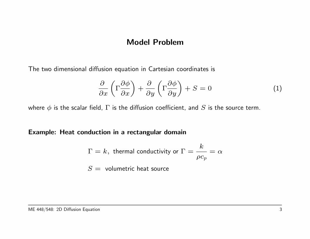
Model Problem
The two dimensional diffusion equation in Cartesian coordinates is
∂
∂x
(Γ∂φ
∂x
)+∂
∂y
(Γ∂φ
∂y
)+ S = 0 (1)
where φ is the scalar field, Γ is the diffusion coefficient, and S is the source term.
Example: Heat conduction in a rectangular domain
Γ = k, thermal conductivity or Γ =k
ρcp= α
S = volumetric heat source
ME 448/548: 2D Diffusion Equation 3

2D Cartesian Finite Volume Mesh
x
y
1 2 nx
i = 0 2j = 0
2
3
3 nx
ny
xu(1) = 0
x(i)
y(j)
xu(i)
1
yv(j)
yv(ny+1)
xu(nx+1)
1
nx+1 nx+2
nx ny
yv(1) = 0
Interior node
Boundary node
Ambiguous corner node
ME 448/548: 2D Diffusion Equation 4

Finite Volume Mesh: Compass Point Notation
Nodes are labelled with their position
relative to the typical point “P”.
N
S
EW
x
y
Capital letters designate node locations.
N, S, E, W are the names of north,
south, east and west neighbors.
φN , φS, φE, φW are the values of φ at
the north, south, east and west neighbor
nodes.
Use of compass point names simplifies
the algebra. For example the value of φ
at point N is φN or φi,j+1, but φN is
simpler to write.
Compass point notation is an historic
convention that does not extend to
unstructured meshes.
ME 448/548: 2D Diffusion Equation 5
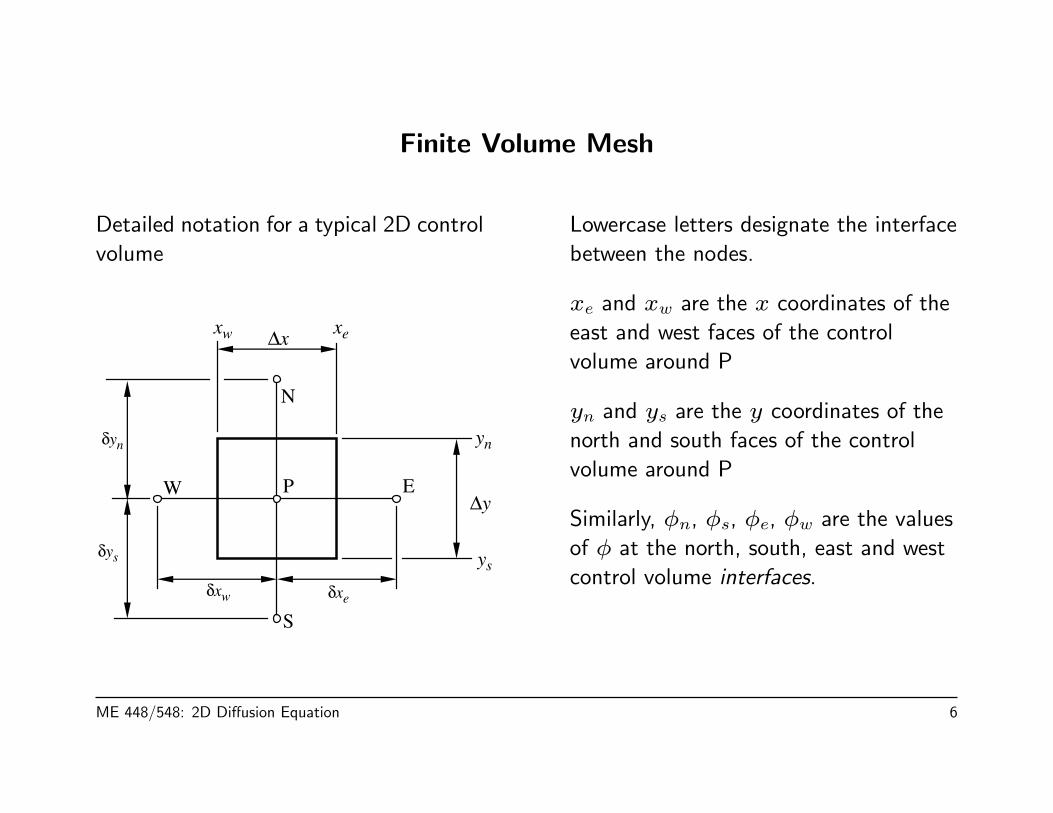
Finite Volume Mesh
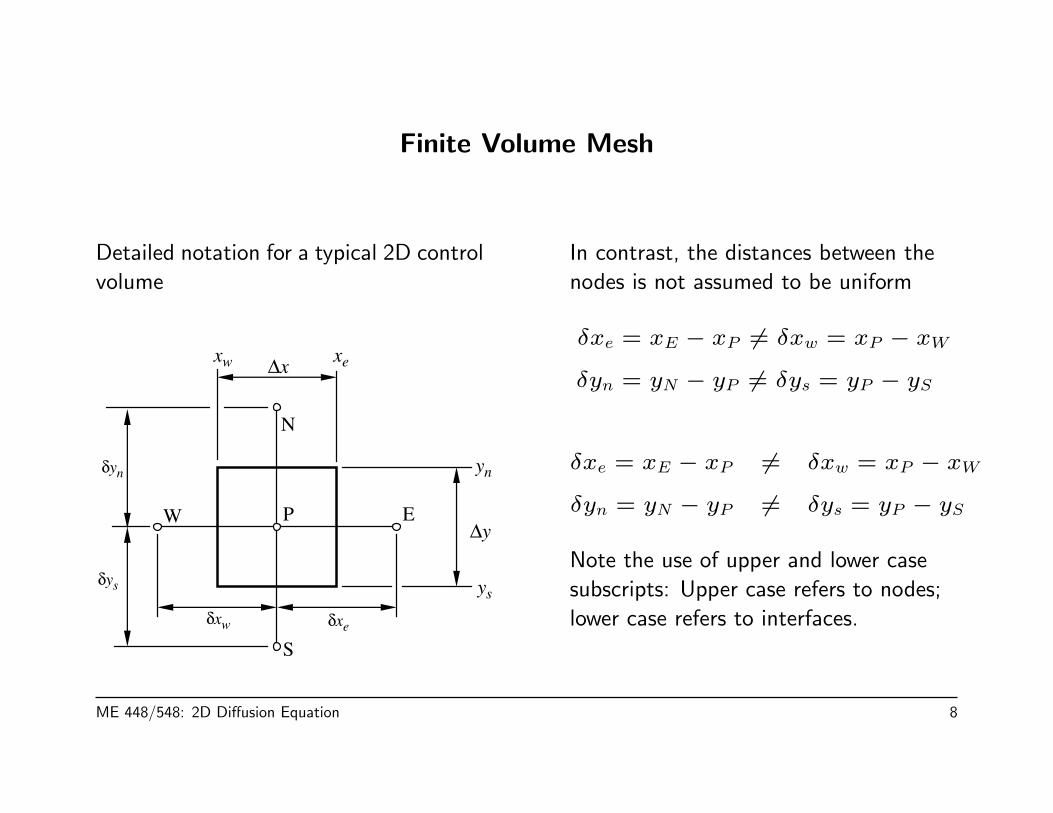
Detailed notation for a typical 2D control
volume
δxw δx
e
S
PW E
N
∆x
∆y
xexw
yn
ys
δys
δyn
Lowercase letters designate the interface
between the nodes.
xe and xw are the x coordinates of the
east and west faces of the control
volume around P
yn and ys are the y coordinates of the
north and south faces of the control
volume around P
Similarly, φn, φs, φe, φw are the values
of φ at the north, south, east and west
control volume interfaces.
ME 448/548: 2D Diffusion Equation 6
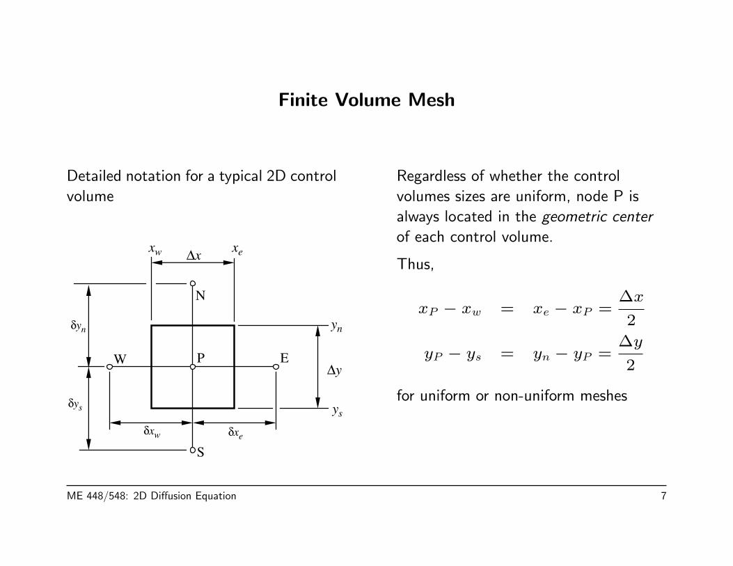
Finite Volume Mesh
Detailed notation for a typical 2D control
volume
δxw δx
e
S
PW E
N
∆x
∆y
xexw
yn
ys
δys
δyn
Regardless of whether the control
volumes sizes are uniform, node P is
always located in the geometric center
of each control volume.
Thus,
xP − xw = xe − xP =∆x
2
yP − ys = yn − yP =∆y
2
for uniform or non-uniform meshes
ME 448/548: 2D Diffusion Equation 7
Finite Volume Mesh
Detailed notation for a typical 2D control
volume
δxw δx
e
S
PW E
N
∆x
∆y
xexw
yn
ys
δys
δyn
In contrast, the distances between the
nodes is not assumed to be uniform
δxe = xE − xP 6= δxw = xP − xWδyn = yN − yP 6= δys = yP − yS
δxe = xE − xP 6= δxw = xP − xWδyn = yN − yP 6= δys = yP − yS
Note the use of upper and lower case
subscripts: Upper case refers to nodes;
lower case refers to interfaces.
ME 448/548: 2D Diffusion Equation 8

Convert the Differential Equation to a Discrete Equation
Integrate over the control volume
∫ yn
ys
∫ xe
xw
∂
∂x
(Γ∂φ
∂x
)dx dy
=
∫ yn
ys
[(Γ∂φ
∂x
)e
−(
Γ∂φ
∂x
)w
]dy
≈[(
Γ∂φ
∂x
)e
−(
Γ∂φ
∂x
)w
]∆y
≈[ΓeφE − φPδxe
− ΓwφP − φWδxw
]∆y
δxw δx
e
S
PW E
N
∆x
∆y
xexw
yn
ys
δys
δyn
The final step is obtained by using central difference approximations for the derivatives at
the interfaces.
ME 448/548: 2D Diffusion Equation 9

Convert the Differential Equation to a Discrete Equation
Integrate the source term ∫ xe
xw
∫ yn
ys
S dy dx ≈ SP∆x∆y (2)
Note: The Control Volume Finite Difference (CVFD) method treats the source term and
diffusion coefficients as piecewise constants. This is a rather crude approximation, say,
compared to allowing the source term and diffusion coefficient to vary linearly within the
control volume.
However, piecewise constant profiles of S and Γ allow the method to be conservative,
i.e., conserving mass or energy, automatically. The conservative nature of the CVFD
method is one of its primary strengths.
ME 448/548: 2D Diffusion Equation 10

Convert the Differential Equation to a Discrete Equation
Putting pieces back into the model equation gives the discrete system of equations
−aSφS − aWφW + aPφP − aEφE − aNφN = b (3)
where
aE =Γe
∆x δxe, aW =
Γw
∆x δxw, aN =
Γn
∆y δyn, aS =
Γs
∆y δys
aP = aE + aW + aN + aS (4)
b = SP (5)
This is not a tridiagonal system of equations.
ME 448/548: 2D Diffusion Equation 11

Non-uniform Γ
Continuity of fluxes at the interface requires
ΓP∂φ
∂x
∣∣∣∣xe−
= ΓE∂φ
∂x
∣∣∣∣xe+
= Γe∂φ
∂x
∣∣∣∣xe
Use central difference approximations
ΓeφE − φPδxe
= ΓPφe − φPδxe−
(6)
ΓeφE − φPδxe
= ΓEφE − φeδxe+
(7)δx
e
material 1 material 2
δxe+
δxe
P E
ME 448/548: 2D Diffusion Equation 12

Non-uniform Γ
Equations 6 and 7 can be rearranged as
φe − φP =δxe−
ΓP
Γe
δxe(φE − φP ) (8)
φE − φe =δxe+
ΓE
Γe
δxe(φE − φP ) (9)
Add Equation 8 and Equation 9
φE − φP =Γe
δxe(φE − φP )
[δxe−
ΓP+δxe+
ΓE
].
δxe
material 1 material 2
δxe+
δxe
P E
Cancel the factor of (φE − φP ) and solve for Γe/δxe to get
Γe
δxe=
[δxe−
ΓP+δxe+
ΓE
]−1
=ΓE ΓP
δxe−ΓE + δxe+ΓP.
ME 448/548: 2D Diffusion Equation 13

Non-uniform Γ
Thus, the diffusion coefficient at the interface that results in flux continuity is
Γe =ΓE ΓP
βΓE + (1− β)ΓP(10)
where
β ≡δxe−
δxe=xe − xPxE − xP
(11)
An analogous derivation gives formulas for Γw, Γn, and Γs.
ME 448/548: 2D Diffusion Equation 14

Solving the System of Equations
Regardless of uniform or variable Γ, the discrete equation has a five-point stencil, and the
discrete equation for any interior node can be written.
−aSφS − aWφW + aPφP − aEφE − aNφN = b (12)
To set up the matrix for this system of equations, we need to re-number the unknowns.
Important: i and j subscripts for the mesh are not the same as the row and
column indices in the system Ax = b.
ME 448/548: 2D Diffusion Equation 15
Solving the System of Equations
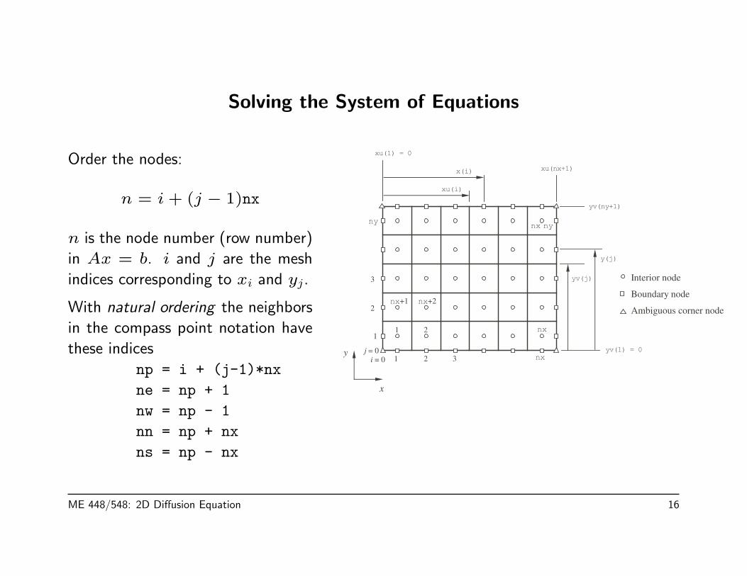
Order the nodes:
n = i+ (j − 1)nx
n is the node number (row number)
in Ax = b. i and j are the mesh
indices corresponding to xi and yj.
With natural ordering the neighbors
in the compass point notation have
these indices
np = i + (j-1)*nx
ne = np + 1
nw = np - 1
nn = np + nx
ns = np - nx
x
y
1 2 nx
i = 0 2j = 0
2
3
3 nx
ny
xu(1) = 0
x(i)
y(j)
xu(i)
1
yv(j)
yv(ny+1)
xu(nx+1)
1
nx+1 nx+2
nx ny
yv(1) = 0
Interior node
Boundary node
Ambiguous corner node
ME 448/548: 2D Diffusion Equation 16

Solving the System of Equations
This leads to a vector of unknowns
φ1,1
φ2,1...
φnx,1φ1,2
φ2,2...
φi,j...
φnx,ny
⇐⇒
φ1
φ2...
φnxφnx+1
φnx+2...
φn...
φN
(13)
ME 448/548: 2D Diffusion Equation 17
Solving the System of Equations
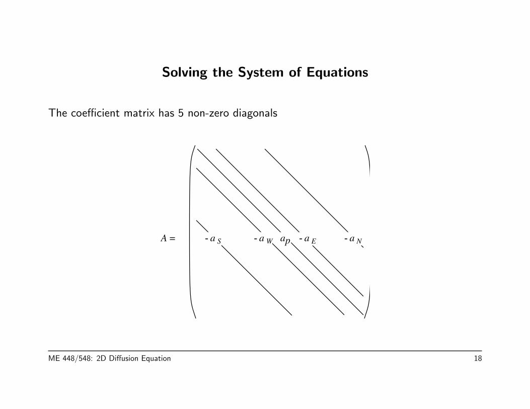
The coefficient matrix has 5 non-zero diagonals
A = a S apa W a E a N
ME 448/548: 2D Diffusion Equation 18
Algorithm for obtaining the numerical solution
1. Define physical parameters: Lx, Ly, Γ(x, y) and boundary conditions
2. Define the mesh: nx and ny if uniform
3. Compute the coefficient matrix
4. Solve the system of equations Aφ = b, where φ is the vector of unknowns.
5. Post-process to visualize the solution
The Poisson equation is steady. Each step is performed only once.
ME 448/548: 2D Diffusion Equation 19
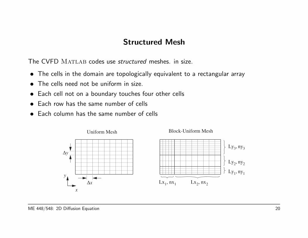
Structured Mesh
The CVFD Matlab codes use structured meshes. in size.
• The cells in the domain are topologically equivalent to a rectangular array
• The cells need not be uniform in size.
• Each cell not on a boundary touches four other cells
• Each row has the same number of cells
• Each column has the same number of cells
Uniform Mesh Block-Uniform Mesh
Lx1, nx1 Lx2, nx2
Ly1, ny1
Ly2, ny2
Ly3, ny3
x
y
∆x
∆y
ME 448/548: 2D Diffusion Equation 20

Boundary Conditions (part 1)
Boundarytype
BoundaryCondition Post-processing in fvpost
1 Specified T Compute q′′ from discrete approximation to Fourier’s law.
q′′
= kTb − Tixb − xi
where Ti and Tb are interior and boundary temperatures, respectively.
2 Specified q′′ Compute Tb from discrete approximation to Fourier’s law.
Tb = Ti + q′′ xb − xi
kwhere Ti and Tb are interior and boundary temperatures, respectively.
ME 448/548: 2D Diffusion Equation 21
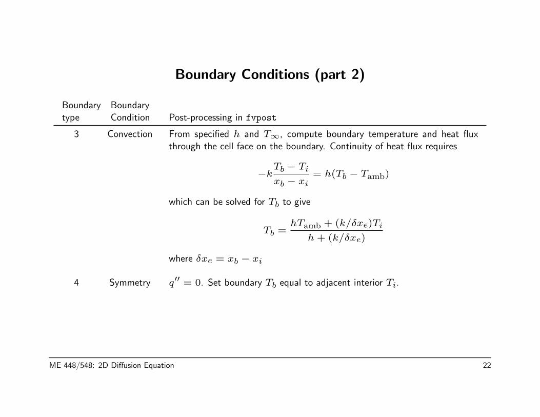
Boundary Conditions (part 2)
Boundarytype
BoundaryCondition Post-processing in fvpost
3 Convection From specified h and T∞, compute boundary temperature and heat fluxthrough the cell face on the boundary. Continuity of heat flux requires
−kTb − Tixb − xi
= h(Tb − Tamb)
which can be solved for Tb to give
Tb =hTamb + (k/δxe)Ti
h+ (k/δxe)
where δxe = xb − xi
4 Symmetry q′′ = 0. Set boundary Tb equal to adjacent interior Ti.
ME 448/548: 2D Diffusion Equation 22

Matlab codes for obtaining the numerical solution
A set of general purpose codes has been written to facilitate experimentation with the
CVFD method.
Algorithm Tasks Core Routines
Define the mesh fvUniformMesh or
fvUniBlockMesh
Define boundary conditions
Compute finite-volume coefficients for interior cells fvcoef
Adjust coefficients for boundary conditions fvbc
Solve system of equations
Assemble coefficient matrix fvAmatrix
Solve
Compute boundary values and/or fluxes fvpost
Plot results
ME 448/548: 2D Diffusion Equation 23
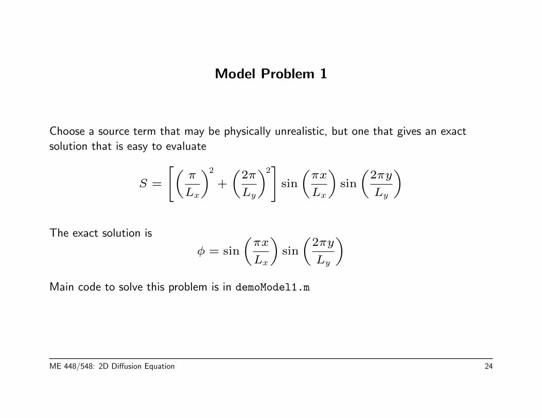
Model Problem 1
Choose a source term that may be physically unrealistic, but one that gives an exact
solution that is easy to evaluate
S =
[(π
Lx
)2
+
(2π
Ly
)2]
sin
(πx
Lx
)sin
(2πy
Ly
)
The exact solution is
φ = sin
(πx
Lx
)sin
(2πy
Ly
)Main code to solve this problem is in demoModel1.m
ME 448/548: 2D Diffusion Equation 24

Model Problem 1
The exact solution is
φ = sin
(πx
Lx
)sin
(2πy
Ly
)
0
0.5
1
00.2
0.40.6
0.81
0
0.5
1
1.5
2
yx
ME 448/548: 2D Diffusion Equation 25

Solutions to Model Problem 1 Show Correct Truncation Error
The local truncation error at each node is
ei ∼ O(∆x2).
Since the exact solution is known we can
compute
‖e‖2
N=
√∑e2i
N∼√Ne2
N=
e√N.
where N = nxny is the total number of
interior nodes in the domain, and e is the
average truncation error per node.10
−310
−210
−110
010
−8
10−7
10−6
10−5
10−4
10−3
10−2
10−1
∆ x
Me
asu
red
err
or
Measured
Theoretical error ~ (∆ x)3
Since ei ∼ O(∆x2), N ∼ n2x, and ∆x = Lx/(nx + 1), we can estimate
‖e‖2
N∼
e√N
=O(∆x2)
nx=O(L2x/(nx + 1)2
)nx
∼ O(
1
nx
)3
= O(∆x3).
ME 448/548: 2D Diffusion Equation 26

Model Problem 2
Uniform source term: S = 1.
Analytical solution is an infinite
series
Code in demoModel2.m
0
0.5
1
00.2
0.40.6
0.81
0
0.01
0.02
0.03
0.04
0.05
0.06
0.07
0.08
yx
ME 448/548: 2D Diffusion Equation 27
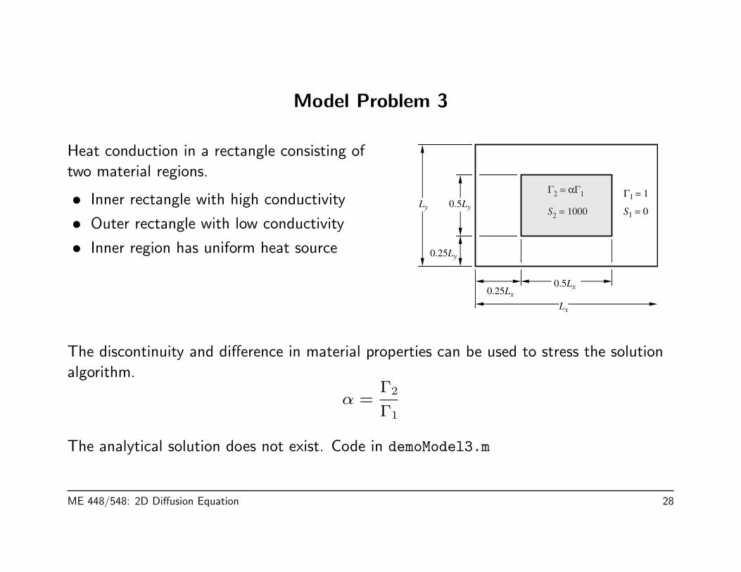
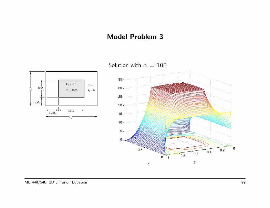
Model Problem 3
Heat conduction in a rectangle consisting of
two material regions.
• Inner rectangle with high conductivity
• Outer rectangle with low conductivity
• Inner region has uniform heat source
0.25Lx
0.25Ly
0.5Ly
0.5Lx
Lx
Ly
Γ1 = 1
S1 = 0
Γ2 = αΓ
1
S2 = 1000
The discontinuity and difference in material properties can be used to stress the solution
algorithm.
α =Γ2
Γ1
The analytical solution does not exist. Code in demoModel3.m
ME 448/548: 2D Diffusion Equation 28
Model Problem 3
0.25Lx
0.25Ly
0.5Ly
0.5Lx
Lx
Ly
Γ1 = 1
S1 = 0
Γ2 = αΓ
1
S2 = 1000
Solution with α = 100
0
0.5
1
00.2
0.40.6
0.81
0
5
10
15
20
25
30
35
yx
ME 448/548: 2D Diffusion Equation 29

Model Problem 4: Fully Developed Flow in a Rectangular Duct
For simple fully-developed flow the governing equation for the axial velocity w is
µ
[∂2w
∂x2+∂2w
∂y2
]−dp
dz= 0
This corresponds to the generic model equation with
φ = w, Γ = µ (= constant), S = −dp
dz.
ME 448/548: 2D Diffusion Equation 30

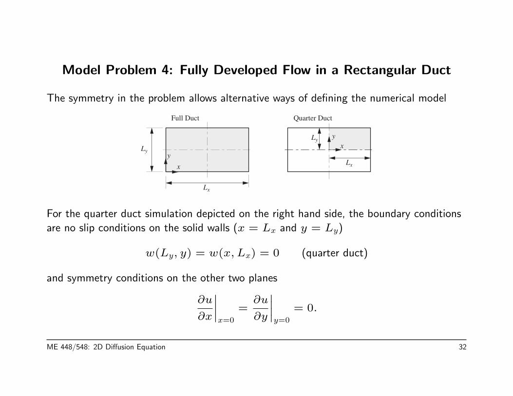
Model Problem 4: Fully Developed Flow in a Rectangular Duct
The symmetry in the problem allows alternative ways of defining the numerical model
Full Duct
x
y
Lx
Ly
Quarter Duct
x
y
Lx
Ly
For the full duct simulation depicted on the left hand side, the boundary conditions are no
slip conditions on all four walls.
w(x, 0) = w(x, Ly) = w(0, y) = w(Lx, y) = 0. (full duct)
ME 448/548: 2D Diffusion Equation 31
Model Problem 4: Fully Developed Flow in a Rectangular Duct
The symmetry in the problem allows alternative ways of defining the numerical model
Full Duct
x
y
Lx
Ly
Quarter Duct
x
y
Lx
Ly
For the quarter duct simulation depicted on the right hand side, the boundary conditions
are no slip conditions on the solid walls (x = Lx and y = Ly)
w(Ly, y) = w(x, Lx) = 0 (quarter duct)
and symmetry conditions on the other two planes
∂u
∂x
∣∣∣∣x=0
=∂u
∂y
∣∣∣∣y=0
= 0.
ME 448/548: 2D Diffusion Equation 32
Related Documents