ISSN 1995-2848 OECD Journal: Economic Studies Volume 2008 © OECD 2008 1 The Contribution of Economic Geography to GDP per Capita by Hervé Boulhol, Alain de Serres and Margit Molnar The authors would like to thank numerous OECD colleagues, in particular Sveinbjörn Blöndal, Sean Dougherty, Jørgen Elmeskov, Christian Gianella, David Haugh, Peter Hoeller, Nick Johnstone, Vincent Koen, Dirk Pilat, Jean-Luc Schneider and Andreas Woergoetter, for their valuable comments as well as Philippe Briard and Martine Levasseur for technical assistance and Caroline Abettan for editorial support. The paper has also benefited from comments by members of the Working party No. 1 of the OECD Economic Policy Committee, as well as the participants to the “The Gravity Model” Conference, Groningen, October 2007. Introduction and main findings . . . . . . . . . . . . . . . . . . . . . . . . . . . . . . . . . . . . 2 General empirical framework . . . . . . . . . . . . . . . . . . . . . . . . . . . . . . . . . . . . . . 4 The basic determinants of GDP per capita . . . . . . . . . . . . . . . . . . . . . . . 4 Benchmark specification and empirical results . . . . . . . . . . . . . . . . . . . 5 Economic distance . . . . . . . . . . . . . . . . . . . . . . . . . . . . . . . . . . . . . . . . . . . . . . . 7 Why proximity matters . . . . . . . . . . . . . . . . . . . . . . . . . . . . . . . . . . . . . . . 7 The distance of OECD countries to world markets . . . . . . . . . . . . . . . . 9 Empirical analysis: Augmented Solow model and proximity . . . . . . . . 13 Transport costs . . . . . . . . . . . . . . . . . . . . . . . . . . . . . . . . . . . . . . . . . . . . . . . . . . 15 Evolution of transport and telecommunications cost indices . . . . . . . 17 Impact of transport costs on openness to trade and GDP per capita . 21 Overall economic impact and policy implications . . . . . . . . . . . . . . . . . . . . . 24 Overall impact . . . . . . . . . . . . . . . . . . . . . . . . . . . . . . . . . . . . . . . . . . . . . . . 24 Policy implications . . . . . . . . . . . . . . . . . . . . . . . . . . . . . . . . . . . . . . . . . . . 25 Conclusions . . . . . . . . . . . . . . . . . . . . . . . . . . . . . . . . . . . . . . . . . . . . . . . . . . . . . 29 Notes . . . . . . . . . . . . . . . . . . . . . . . . . . . . . . . . . . . . . . . . . . . . . . . . . . . . . . . . . . . 30 Bibliography . . . . . . . . . . . . . . . . . . . . . . . . . . . . . . . . . . . . . . . . . . . . . . . . . . . . . 32 Annex: The Augmented Solow Model . . . . . . . . . . . . . . . . . . . . . . . . . . . . . . . . 34

Welcome message from author
This document is posted to help you gain knowledge. Please leave a comment to let me know what you think about it! Share it to your friends and learn new things together.
Transcript
ISSN 1995-2848
OECD Journal: Economic Studies
Volume 2008
© OECD 2008
The Contribution of Economic Geography to GDP per Capita
byHervé Boulhol, Alain de Serres and Margit Molnar
The authors would like to thank numerous OECD colleagues, in particular
Sveinbjörn Blöndal, Sean Dougherty, Jørgen Elmeskov, Christian Gianella, David Haugh,
Peter Hoeller, Nick Johnstone, Vincent Koen, Dirk Pilat, Jean-Luc Schneider and
Andreas Woergoetter, for their valuable comments as well as Philippe Briard and
Martine Levasseur for technical assistance and Caroline Abettan for editorial support. The
paper has also benefited from comments by members of the Working party No. 1 of the
OECD Economic Policy Committee, as well as the participants to the “The Gravity Model”
Conference, Groningen, October 2007.
Introduction and main findings . . . . . . . . . . . . . . . . . . . . . . . . . . . . . . . . . . . . 2
General empirical framework . . . . . . . . . . . . . . . . . . . . . . . . . . . . . . . . . . . . . . 4
The basic determinants of GDP per capita . . . . . . . . . . . . . . . . . . . . . . . 4
Benchmark specification and empirical results . . . . . . . . . . . . . . . . . . . 5
Economic distance . . . . . . . . . . . . . . . . . . . . . . . . . . . . . . . . . . . . . . . . . . . . . . . 7
Why proximity matters . . . . . . . . . . . . . . . . . . . . . . . . . . . . . . . . . . . . . . . 7
The distance of OECD countries to world markets . . . . . . . . . . . . . . . . 9
Empirical analysis: Augmented Solow model and proximity . . . . . . . . 13
Transport costs . . . . . . . . . . . . . . . . . . . . . . . . . . . . . . . . . . . . . . . . . . . . . . . . . . 15
Evolution of transport and telecommunications cost indices . . . . . . . 17
Impact of transport costs on openness to trade and GDP per capita . 21
Overall economic impact and policy implications . . . . . . . . . . . . . . . . . . . . . 24
Overall impact . . . . . . . . . . . . . . . . . . . . . . . . . . . . . . . . . . . . . . . . . . . . . . . 24
Policy implications . . . . . . . . . . . . . . . . . . . . . . . . . . . . . . . . . . . . . . . . . . . 25
Conclusions . . . . . . . . . . . . . . . . . . . . . . . . . . . . . . . . . . . . . . . . . . . . . . . . . . . . . 29
Notes . . . . . . . . . . . . . . . . . . . . . . . . . . . . . . . . . . . . . . . . . . . . . . . . . . . . . . . . . . . 30
Bibliography . . . . . . . . . . . . . . . . . . . . . . . . . . . . . . . . . . . . . . . . . . . . . . . . . . . . . 32
Annex: The Augmented Solow Model . . . . . . . . . . . . . . . . . . . . . . . . . . . . . . . . 34
1
THE CONTRIBUTION OF ECONOMIC GEOGRAPHY TO GDP PER CAPITA
Introduction and main findingsOver the past several years, the OECD has quantified the impact of structural policies
on employment, productivity and GDP per capita (e.g. OECD, 2003, 2006). The results from
these studies, which have built on a vast academic literature, have contributed to a better
understanding of the main channels linking policies to labour and product market
outcomes in OECD countries. In doing so, they have also underscored the limits to the
understanding of economic growth: only a limited part of the cross-country dispersion in
GDP levels and growth rates can be explained by quantifiable policy levers, at least on the
basis of standard macro-growth regression analysis.
This paper examines how much of the cross-country dispersion in economic
performance can be accounted for by economic geography factors. To do so, an augmented
Solow model is used as a benchmark. The choice is motivated by the fact that this model
has served as the basic framework in previous work on the determinants of growth,
thereby ensuring some continuity. It has long been recognised, however, that while
providing a useful benchmark to assess the contributions of factor accumulation as a
source of differences in GDP per capita, the basic Solow growth model ignores potentially
important determinants. For instance, it leaves a large portion of growth to be explained by
the level of technology, which is assumed to grow at a rate set exogenously.
In order to bridge some of the gaps, extensions of the model in the literature have
generally taken four types of (partly related) directions: i) R&D and innovation, ii) goods
market integration and openness to international trade, iii) quality of institutions, and
iv) economic geography. The focus of this paper is on economic geography, although this is
not totally independent from the other factors, in particular international trade. More
specifically, for the purpose of this study, the concept of economic geography is examined
through the proximity to areas of dense economic activity.
The key point of this aspect of geography is the recognition that proximity may have a
favourable impact on productivity, through various channels operating via product and
labour markets. In the case of product markets, one of the key channels is that proximity
induces stronger competition between producers, thus encouraging efficient use of
resources and innovation activity. Another is that an easy access to a large market for
consumers and suppliers of intermediate goods allows for the exploitation of increasing
returns to scale. Furthermore, the presence of large markets allows for these scale effects
to be realised without adversely affecting competition. The scope for exploiting higher
returns to scale is hampered by distance to major markets, both within and across
countries, due to transportation costs. Transportation costs also reduce the scope for
specialisation according to comparative advantage, another important driver of gains from
trade along with the ability to reap scale economies.
While the economic geography literature focuses mainly on trade linkages, a parallel
literature on urban and spatial economics puts more emphasis on agglomeration
externalities as a benefit from operating in an area of dense economic activity. Such
OECD JOURNAL: ECONOMIC STUDIES – VOLUME 2008 – ISSN 1995-2848 – © OECD 20082
THE CONTRIBUTION OF ECONOMIC GEOGRAPHY TO GDP PER CAPITA
externalities may include economies of scale related to infrastructure and other public
services, as well as the potential gains associated with the access to a large pool of workers,
and localised knowledge spillovers. In principle, it is possible to provide some
quantification of these benefits, using standard measures of economic density, such as the
share of population living in cities. In practice, such measures are highly endogenous to
economic development and finding appropriate instruments to address the endogeneity
problem is beyond the scope of this paper. As a result, this aspect is only examined in a
very tentative way in the final section of the paper.
The empirical strategy pursued in the paper is as follows. In the next section, the
augmented Solow model, which is used as the basic framework, is first briefly described
and estimated both in level and in error-correction forms, over a sample of 21 OECD
countries over the period 1970-2004. The influence of proximity to major markets on GDP
per capita is then investigated in the following section, introducing in the benchmark
model various indicators of distance to markets, such as measures of market potential,
market and supplier access, as well as the sum of distances to world markets and
population density. The various measures of distance to markets are all found to have a
statistically significant effect on GDP per capita, with the exception of population density.
The estimated economic impact varies somewhat across specifications, but it is far from
negligible. For instance, the lower access to markets relative to the OECD average could
contribute negatively to GDP per capita by as much as 11% in Australia and New Zealand.
Conversely, the benefit from a favourable location could be as high as 6-7% of GDP in the
case of Belgium and the Netherlands.
Later in the text, the impact of distance is alternatively examined via the more specific
channel of transportation and telecommunication costs. To this end, broad indicators of
weight-based transportation costs covering maritime, air and road shipping have been
constructed for 21 OECD countries over the period 1973-2004, along with an indicator of the
cost of international telecommunications. Based on these indicators, there is little
evidence that the importance of distance in the transportation of goods has diminished
during the past two or three decades (though transport costs may have fallen relative to the
value of transported goods). In contrast, the cost of international telecommunications has
fallen in all countries to the point where it is basically no longer significant anywhere.
Overall, transportation costs are found to have a negative and significant effect on GDP per
capita through their effect on international trade. Based on these estimates, differences in
transport costs relative to the OECD average contribute to reduce GDP per capita by
between 1.0% and 4.5% in Australia and New Zealand. At the other end, the lower transport
costs for Canada and the United States contribute to raise GDP per capita relative to the
average OECD country, but only by a small margin varying between 0.5% and 2.5%. The
quantitatively smaller effects than those found on the basis of measures of economic
distance are consistent with transportation costs being only one aspect of costs related to
distance.
Most of the geography factors discussed in this paper cannot be influenced by policy
or are only affected by policy in indirect ways. Nevertheless, a number of policy issues are
addressed in the penultimate section, which also provides a summary of the combined
economic impact of the geographic variables used in the empirical analysis.
OECD JOURNAL: ECONOMIC STUDIES – VOLUME 2008 – ISSN 1995-2848 – © OECD 2008 3
THE CONTRIBUTION OF ECONOMIC GEOGRAPHY TO GDP PER CAPITA
General empirical frameworkA basic empirical framework is required in order to assess the importance of economic
geography in determining GDP per capita. Against the background of earlier OECD analysis
in this area, this section briefly reviews the basic determinants of GDP per capita, discusses
alternative specifications in terms of levels and changes over time, and reports the results
of an empirical analysis using only the basic determinants. The remainder of the paper will
then examine whether economic geography variables can account for some of the variance
in GDP per capita left unexplained by the basic determinants.
The basic determinants of GDP per capita
The empirical framework used to assess the influence of economic geography
determinants is the Solow (1956) model augmented with human capital. The model has
been widely used in the empirical growth literature, owing largely to its simplicity and
flexibility. For instance, despite being derived from a specific framework, the empirical
version of model is sufficiently general to be consistent with some endogenous growth
models (Arnold et al., 2007).
The Solow model has been widely used as a theoretical framework to explain
differences across countries in income levels and growth patterns. The model is based on
a simple production function with constant returns-to-scale technology. In the augmented
version of the model (Mankiw, Romer and Weil, 1992), output is a function of human and
physical capital, as well as labour (working-age population) and the level of technology.
Under a number of assumptions about the evolution of factors of production over time, the
model can be solved for its long-run (steady-state) equilibrium whereby the path of output
per capita is determined by the rates of investment in physical and human capital, the level
of technology, and the growth rate of population (see Annex for a detailed derivation). In
the steady-state, the growth of GDP per capita is driven solely by technology, which is
assumed to grow at a (constant) rate set exogenously in the basic model.
The long-run relationship derived from the augmented Solow model can be estimated
either directly in its level form, or through a specification that explicitly takes into account
the dynamic adjustment to the steady state. Estimates of the long-run relationship in static
form have been used in the literature (e.g. Mankiw, Romer and Weil, 1992; Hall and Jones,
1999; Bernanke and Gürkaynak, 2001), in particular in studies focusing on income level
differentials across countries. However, since the model has often been used in the
empirical growth literature to examine issues of convergence, some form of dynamic
specification has been more common. The two types of specification – static or dynamic –
can be expected to yield similar results if countries are not too far from their steady states
or if deviations from the latter are not too persistent.
In principle, a dynamic specification is preferable, even when the interest is mainly on
the identification of long-run determinants. This is because persistent deviations from
steady state are more likely to lead to biased estimates of the long-run parameters in static
regressions, especially when the time-series dimension of the sample is relatively short. In
practice, estimating dynamic panel equations is also fraught with econometric problems
(Durlauf and Quah, 1999). Furthermore, a major drawback with the most common
techniques based on dynamic fixed-effect estimators is that only the intercepts are
allowed to vary across countries, implying that all countries converge to their steady-state
at the same speed, an assumption unlikely to hold even among developed countries.1
OECD JOURNAL: ECONOMIC STUDIES – VOLUME 2008 – ISSN 1995-2848 – © OECD 20084
THE CONTRIBUTION OF ECONOMIC GEOGRAPHY TO GDP PER CAPITA
To address the latter issue, previous studies have relied on the Pooled Mean Group
(PMG) estimator, which allows for short-run coefficients and the speed of adjustment to
vary across countries, while imposing homogeneity on long-run coefficients (OECD, 2003).
However, even though the PMG estimation technique is intuitively appealing and perhaps
the most suitable under some conditions, it is not without limitations especially when
such conditions are not met. For instance, due to the large number of parameters and the
non-linear constraints, the maximum likelihood estimation technique is prone to
problems of convergence on local optima. And, experience suggests that parameter
estimates can be particularly sensitive in presence of multi-collinearity among regressors,
with some parameter values being in such cases too large (and unstable) to be plausible.
For the purpose of this study, the model is first re-estimated with only the basic
determinants included in the specification, i.e. proxies for investment in physical and
human capital, population growth and technical progress. Then, a number of determinants
are added to the benchmark specification throughout the rest of the paper, but the set of
additional variables is limited to those related to economic geography factors. One
exception is the measure of exposure to international trade which, given the importance of
geography on trade, is used to assess the impact of transportation costs on GDP per capita
(see later in the text). The reason for leaving other potential variables out is essentially one
of parsimony, i.e. to limit the number of specifications, which quickly runs up as each
additional determinant is considered.2 However, this implies that potentially significant
control variables are not included, with the risk that this entails in terms of biases and
robustness of the results as regards the determinants of economic geography. In order to
minimise those risks, all specifications include various combinations of country and year
fixed-effects and/or linear time trends, all of which are introduced in part to capture
omitted variables.
Benchmark specification and empirical results
The empirical version of the augmented-Solow model is re-estimated over a panel
data set comprising 21 countries and 35 years of observations (1970-2004). In what will
serve as the reference model for the rest of the paper, the level of GDP per working-age
person in country i and year t (yit) is regressed on the rate of investment in the total
economy (sK,it), the average number of years of schooling of the population aged 25-64,
which is used as a proxy for the stock of human capital (hcit)3 and the growth rate of
population (nit) augmented by a constant factor introduced as a proxy for the sum of the
trend growth rate of technology and the rate of capital depreciation (g + d), with all
variables expressed in logs.4 Technological progress is captured alternatively by a linear
time trend or time dummies.
The results presented in this paper are based on both a level specification, using a
least-square estimator (that corrects for heteroskedasticity and contemporaneous
correlations), and an error correction specification, using the pooled mean group (PMG)
estimator. Due to persistence in the series, control for first-order serial correlation is
systematically made when the level specification is estimated. The functional forms of the
OECD JOURNAL: ECONOMIC STUDIES – VOLUME 2008 – ISSN 1995-2848 – © OECD 2008 5
THE CONTRIBUTION OF ECONOMIC GEOGRAPHY TO GDP PER CAPITA
equations estimated in level and error-correction forms are respectively specified as
follows (see Annex for derivation):
Level specification (AR1)
(1)
Error-correction specification (Pooled Mean Group)
(2)
where ei and et are country and year fixed-effects, respectively, and t is a linear time trend.
The parameters , , , and are the long-run parameters on the three basic determinants
and the time trend. The parameter is the first-order autocorrelation coefficient used in
the level specification.5 The other parameters capture short-run dynamics and will not be
reported in the table of results. Finally, uit and it are the residuals.
The results from re-estimating the empirical version of the augmented-Solow model
are presented in Table 1. The first three columns refer to the level specification and the last
two are based on the error-correction specification. Focusing on the level specification, the
Table 1. Basic framework: Regression resultsAugmented-Solow model1
Dependant variable GDP per capita
Level AR(1) Level AR(1) Level AR(1)Error
correction PMGError
correction PMG
(1) (2) (3) (4) (5)
Common parameters
Physical capital 0.184*** 0.156*** 0.199*** 0.292*** 0.572***
(0.019) (0.024) (0.017) (0.030) (0.059)
Human capital 0.334*** 0.792*** –0.063 0.861*** –0.006
(0.127) (0.053) (0.156) (0.199) (0.189)
Population growth2 –0.006 –0.016 –0.003 –0.392*** –0.661***
(0.018) (0.028) (0.018) (0.067) (0.101)
Time trend 0.015***
(0.002)
Rho3 0.884 0.911 0.775
Country-specific parameters
Lambda4 –0.190*** –0.086***
(0.025) (0.017)
Time trend No No Yes Yes No
Fixed effects
Country Yes No Yes Yes Yes
Year Yes Yes Yes No No
Sample size
Total number of observations 696 696 696 695 695
Number of countries 21 21 21 21 21
Note: Standard errors are in parentheses. *: significant at 10% level; ** at 5% level; *** at 1% level.1. The functional forms corresponding to the “level” and “error-correction” specifications are reported earlier in the
text. In the level specification, standard errors are robust to heteroscedasticity and to contemporaneouscorrelation across panels. In the error-correction specification, only long term parameters are reported.
2. The population growth variable is augmented by a constant factor (g + d) designed to capture trend growth intechnology and capital depreciation. This constant factor is set at 0.05 for all countries.
3. Rho is the first-order auto-correlation parameter.4. The parameter lambda is the average of the country-specific speed adjustment parameter, i.
...,.
)(....
1
,
diiuuueetdgnLogh cLogh cLogsLogyLog
i ti ti ti t
i ttiii ti ti ti tKi t
εερ
ςγϕβα
+=
+++++++Δ++=
−
( )[ ]i tiii tii tii tKi
i ti ti tKi tii t
tedgnLogah cLogasLogadgnLogh cLogsLogyLogyLog
εςγβαλ
+++++Δ+Δ+Δ+++++−−=Δ −
.)(...)(....
21,0
,1
OECD JOURNAL: ECONOMIC STUDIES – VOLUME 2008 – ISSN 1995-2848 – © OECD 20086
THE CONTRIBUTION OF ECONOMIC GEOGRAPHY TO GDP PER CAPITA
coefficient on human capital is quite sensitive to the control for fixed effects and or time
trends. In particular, it comes out significantly higher when country fixed effects are
excluded (column 2), suggesting that an important part of the information contained in the
average number of years of schooling is related to differences in average levels across
countries. Moreover, it completely drops out when country-specific time trends are
included in the regression in addition to country- and year-fixed effects (column 3).
Turning to the error-correction specification, the results shown in the fourth column
are similar to those obtained in the earlier OECD analysis based on an almost identical
specification (with country fixed effects and country-specific parameters on the time
trend) and the same estimation method (PMG).6 The speed of adjustment parameter
suggests rapid convergence to the steady-state, a result which is influenced by the
introduction of country-specific time trend parameters.7 Also, the parameter estimate on
human capital suggests a strong effect, with one extra year of schooling leading to an
increase in GDP per capita by around 8% in the long run for the average OECD country.
However, here again, the significance of the human capital coefficient depends on whether
or not the trend is assumed to be common or country specific (column 5).8
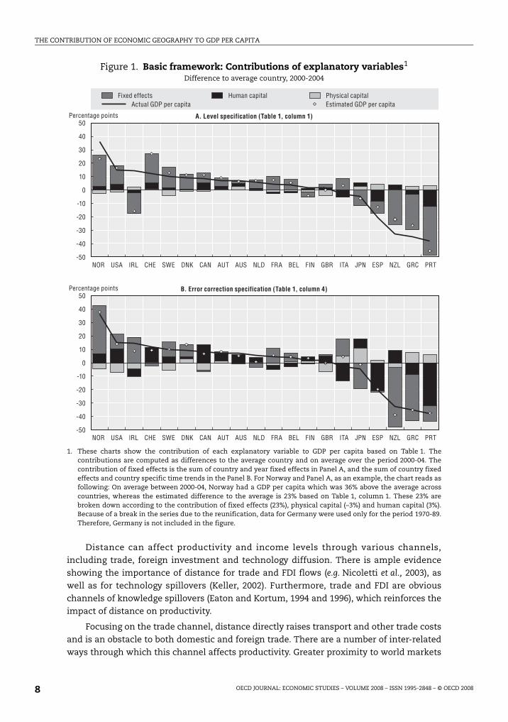
Figure 1 presents the contribution of physical capital, human capital and fixed effects
to the gap in GDP per capita relative to the average OECD country and on average over the
2000-04 period.9 The results presented in the two panels are based on the specifications
shown in columns 1 and 4, respectively. Not surprisingly, the contribution of physical and
human capital is small relative to that of the fixed effects. Indeed, the latter account for
72% and 87% of the GDP per capita variance (over this average period) for the level and the
error correction specification respectively. Some of the highest fixed effects are in both
specifications recorded for Norway and, to a lesser extent, the United States and Sweden.
Portugal, Greece, New Zealand and Japan have the largest negative effects. The position of
Ireland and Switzerland is particularly sensitive to whether common or country-specific
time trends are introduced.
The rest of the paper investigates whether some of these large fixed effects can be
accounted for by indicators of economic geography and, more generally, the extent to
which such indicators can explain part of income levels which is not explained by the usual
determinants.
Economic distanceIn this section, different measures of proximity to markets or centrality are introduced
and tested in the empirical analysis as potential determinants of GDP per capita. Some of
them are simple measures based on GDP, country size, population and distances vis-à-vis
other countries. The others are model-based measures derived from bilateral trade flows.
Why proximity matters
The role of geographic distance and the influence of neighbouring countries have
largely been neglected in traditional growth theory which relies essentially on national
characteristics, e.g. factor endowments and technological progress. Yet, the clustering of
economic activities is a well-known phenomenon that raises questions about the extent to
which the proximity to high-income neighbours matters for a country’s own income. The
development process might indeed be hindered in countries that are distant from centres
of economic activities.
OECD JOURNAL: ECONOMIC STUDIES – VOLUME 2008 – ISSN 1995-2848 – © OECD 2008 7
THE CONTRIBUTION OF ECONOMIC GEOGRAPHY TO GDP PER CAPITA
Distance can affect productivity and income levels through various channels,
including trade, foreign investment and technology diffusion. There is ample evidence
showing the importance of distance for trade and FDI flows (e.g. Nicoletti et al., 2003), as
well as for technology spillovers (Keller, 2002). Furthermore, trade and FDI are obvious
channels of knowledge spillovers (Eaton and Kortum, 1994 and 1996), which reinforces the
impact of distance on productivity.
Focusing on the trade channel, distance directly raises transport and other trade costs
and is an obstacle to both domestic and foreign trade. There are a number of inter-related
ways through which this channel affects productivity. Greater proximity to world markets
Figure 1. Basic framework: Contributions of explanatory variables1
Difference to average country, 2000-2004
1. These charts show the contribution of each explanatory variable to GDP per capita based on Table 1. Thecontributions are computed as differences to the average country and on average over the period 2000-04. Thecontribution of fixed effects is the sum of country and year fixed effects in Panel A, and the sum of country fixedeffects and country specific time trends in the Panel B. For Norway and Panel A, as an example, the chart reads asfollowing: On average between 2000-04, Norway had a GDP per capita which was 36% above the average acrosscountries, whereas the estimated difference to the average is 23% based on Table 1, column 1. These 23% arebroken down according to the contribution of fixed effects (23%), physical capital (–3%) and human capital (3%).Because of a break in the series due to the reunification, data for Germany were used only for the period 1970-89.Therefore, Germany is not included in the figure.
NOR USA IRL CHE SWE DNK CAN AUT AUS NLD FRA BEL FIN GBR ITA JPN ESP NZL GRC PRT
50
40
30
20
10
0
-10
-20
-30
-40
-50
NOR USA IRL CHE SWE DNK CAN AUT AUS NLD FRA BEL FIN GBR ITA JPN ESP NZL GRC PRT
50
40
30
20
10
0
-10
-20
-30
-40
-50
Percentage points A. Level specification (Table 1, column 1)
Percentage points B. Error correction specification (Table 1, column 4)
Fixed effects Human capital Physical capitalActual GDP per capita Estimated GDP per capita
OECD JOURNAL: ECONOMIC STUDIES – VOLUME 2008 – ISSN 1995-2848 – © OECD 20088
THE CONTRIBUTION OF ECONOMIC GEOGRAPHY TO GDP PER CAPITA
increases the opportunity to concentrate resources in activities of comparative advantage.
It also encourages specialisation of firms that can attain efficient scale and more generally
exploit increasing returns in specific fields of production. Moreover, stronger competition
pressures force companies to use available inputs efficiently and encourage them to
innovate and maintain a competitive advantage.
In addition to influencing GDP per capita via its impact on technical efficiency,
distance can also affect external terms of trade. A relatively remote and sparsely populated
country has to internalise transport costs into producer prices of tradeable goods in order
to remain competitive in world markets or otherwise suffer lower sales. Because, by
definition, the factor prices of mobile factors tend to be equalised across locations, the
costs of remoteness are born by the immobile factors, i.e. mostly labour in an international
perspective. Indeed, even if technologies are the same everywhere, firms in more remote
countries can only afford to pay relatively lower wages (Redding and Venables, 2004).
In addition to its direct impact on incomes, geography might have an influence
through other factors such as physical or human capital. Returns to physical and human
capital might be higher in countries having a better access to large markets (Redding and
Scott, 2003). In turn, a high return to skills increases the incentive to invest. As regards
human capital, Redding and Scott provide some evidence that the world’s most peripheral
countries have relatively low levels of education, a feature found also in the case of
European regions (Breinlich, 2007).
The distance of OECD countries to world markets
In this section, four measures of proximity to markets or centrality are constructed
and compared. The first one is population density. The second one depends solely on
distances between countries. The third one is a simple measure based on distances
vis-à-vis other countries and the size of their GDPs, and the last one is a model-based
measure derived from bilateral trade flows. The next section is specifically dedicated to the
effects of economic distance measured by transport costs.
Population density, sum of distances and market potential
Population density, defined as the ratio of population to surface area, is an indicator of
proximity to the domestic market. The higher the density the lower the aggregated
domestic transport costs. However, the critical shortcoming of this measure is its failure to
take into account the effective access to foreign markets.
A simple measure of distance to markets that does so is one based on bilateral
distances. From the perspective of empirical analysis, this measure is attractive because it
is based on exogenous characteristics of geography. Although the sum of the distances of
each country to Tokyo, Brussels and New York has been commonly used in the empirical
literature, the choice of these three locations is arbitrary and creates issues of endogeneity.
Hence, a better alternative is to sum the distances to all countries (Head and Mayer,
2007):
(3)
In order to compute Distsum, the world was divided in 32 areas: Africa, Australia, Austria,
Belgium, Brazil, Canada, China, CIS countries, Denmark, Eastern Europe, Finland, France,
∑=j
i ji dDistsum
OECD JOURNAL: ECONOMIC STUDIES – VOLUME 2008 – ISSN 1995-2848 – © OECD 2008 9
THE CONTRIBUTION OF ECONOMIC GEOGRAPHY TO GDP PER CAPITA
Germany, Greece, Ireland, Italy, Japan, Korea, Latin America (other than Brazil and Mexico),
Mexico, the Middle East, the Netherlands, New Zealand, Norway, Portugal, Spain, Sweden,
Switzerland, Turkey, the United Kingdom, the United States and Asia (other that the
countries already included). Pure distance measures, however, fail to take into account the
size of markets. Moreover, this measure depends on how geographic areas are constructed.
For example, a different picture would be obtained if the European Union was considered as
one entity or, alternatively, the North America was disaggregated into states/provinces.
Therefore, a more refined measure of proximity to markets is market potential, which
is defined as the sum of all countries’ GDP weighted by the inverse of the bilateral distance
(Harris, 1954):
(4)
The market potential measure must take into account, for a given country, the domestic
market and include its own GDP weighted by the inverse of internal distance. Because the
internal distance is generally smaller than external distances, it is associated with a
greater weight and is therefore a sensitive parameter for measures of centrality. The most
commonly used distance indicators combine geodesic capital-to-capital distances
between countries and internal distances based on surface areas.10 It follows that market
potential is likely to be positively correlated with population density due to the domestic
component.
Market and supplier access
Although it is an intuitive indicator of centrality, market potential is an ad-hoc way of
capturing the influence of distance to markets. In particular, the weighting of foreign
markets in the market potential computation is based solely on distances, regardless of the
true accessibility of these markets. In that respect, market potential is a very crude measure
of market access. Indeed, accessibility depends, in addition to distance, on trade policy and
cultural relationships, among other determinants. A better approach consists in looking
not only at the potential, but rather at the actual accessibility to countries’ markets.
A measure based on such an approach has been proposed in the new economic
geography literature, which has revived the concept of proximity to markets and
formalised the role of economic geography in determining income. Using the methodology
proposed by Redding and Venables (2004) and described in Box 1, measures of market and
supplier access have been derived from bilateral trade equations estimated over the
period 1970 and 2005 for the 32 countries/areas covering 98.5% of world trade flows in
goods (see Boulhol and de Serres, 2008, for details).
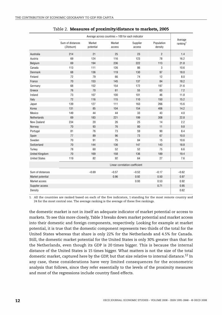
Comparison of the different measures
The various measures of centrality discussed in the previous sub-section have been
computed for most OECD countries and Table 2 reports the computed values for 2005, plus
the average of the country ranking over the different measures. To facilitate the
comparison, each of these measures is scaled such that the average across countries is
100 for each year. The cross-country pattern is reasonably close across indicators. Linear
correlation is especially high, at around 95%, between market potential, market access and
supplier access (and the average ranking). Ranking the countries enables to distinguish five
∑=j i j
ji d
GDPPotentialMarket
OECD JOURNAL: ECONOMIC STUDIES – VOLUME 2008 – ISSN 1995-2848 – © OECD 200810
THE CONTRIBUTION OF ECONOMIC GEOGRAPHY TO GDP PER CAPITA
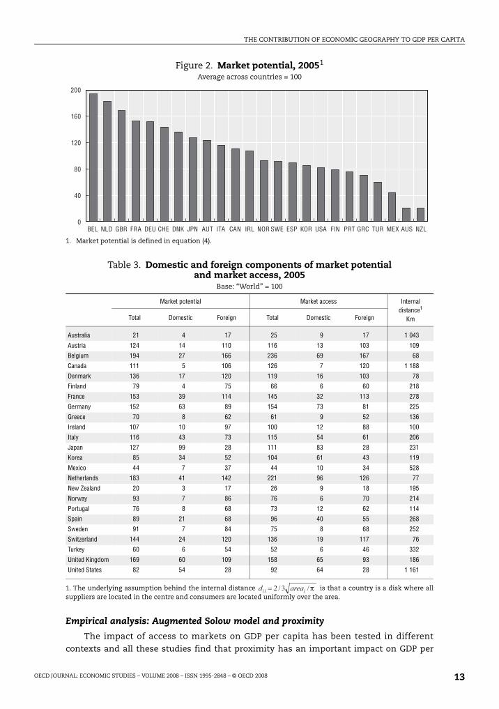
groups, in ascending order and Figure 2 represents this clustering using market potential
for illustration purposes:
● The remote and sparsely populated countries: Australia and New Zealand.
● Low-income peripheral countries.
● High-income peripheral countries, Korea and North America.
● Continental Europe, the United Kingdom and Japan.
● The centrally located and dense economies of Belgium and the Netherlands.
As expected, access measures are negatively correlated to the sum of distances and
positively correlated to population density, suggesting that market and supplier access
encompasses these different geographical dimensions. Besides, population density is an
important factor explaining the position of Japan and Korea at or above what could be
expected from the pure sum-of-distances measure.11
Given the size of its own market, the relative position of the United States in terms of
market potential or market access might look surprising. As shown by the first column in
Table 2 which gives the simplest measure of proximity, one reason is that the United States
is much further from markets than European countries. Another reason is that the size of
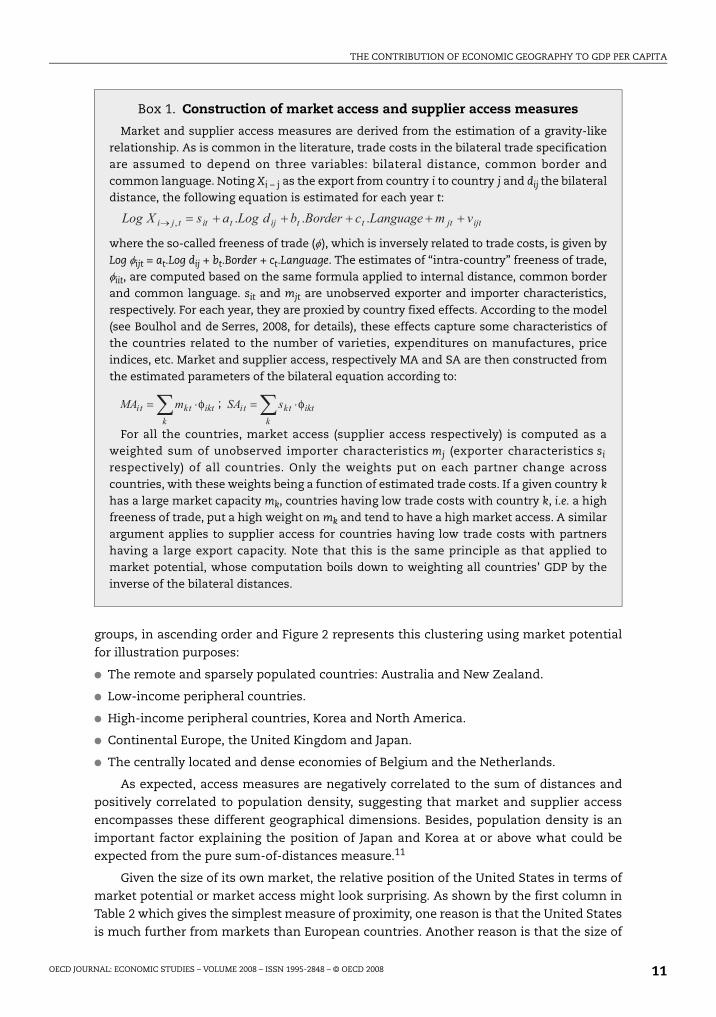
Box 1. Construction of market access and supplier access measures
Market and supplier access measures are derived from the estimation of a gravity-likerelationship. As is common in the literature, trade costs in the bilateral trade specificationare assumed to depend on three variables: bilateral distance, common border andcommon language. Noting Xi – j as the export from country i to country j and dij the bilateraldistance, the following equation is estimated for each year t:
where the so-called freeness of trade (), which is inversely related to trade costs, is given byLog ijt = at.Log dij + bt.Border + ct.Language. The estimates of “intra-country” freeness of trade,iit, are computed based on the same formula applied to internal distance, common borderand common language. sit and mjt are unobserved exporter and importer characteristics,respectively. For each year, they are proxied by country fixed effects. According to the model(see Boulhol and de Serres, 2008, for details), these effects capture some characteristics ofthe countries related to the number of varieties, expenditures on manufactures, priceindices, etc. Market and supplier access, respectively MA and SA are then constructed fromthe estimated parameters of the bilateral equation according to:
;
For all the countries, market access (supplier access respectively) is computed as aweighted sum of unobserved importer characteristics mj (exporter characteristics si
respectively) of all countries. Only the weights put on each partner change acrosscountries, with these weights being a function of estimated trade costs. If a given country khas a large market capacity mk, countries having low trade costs with country k, i.e. a highfreeness of trade, put a high weight on mk and tend to have a high market access. A similarargument applies to supplier access for countries having low trade costs with partnershaving a large export capacity. Note that this is the same principle as that applied tomarket potential, whose computation boils down to weighting all countries’ GDP by theinverse of the bilateral distances.
ijtj ttti jti ttji vmLanguagecBorderbdLogasXLog +++++=→ ...,
∑ ⋅=k
iktk ti t mM A φ ∑ ⋅=k
iktk ti t sS A φ
OECD JOURNAL: ECONOMIC STUDIES – VOLUME 2008 – ISSN 1995-2848 – © OECD 2008 11
THE CONTRIBUTION OF ECONOMIC GEOGRAPHY TO GDP PER CAPITA
the domestic market is not in itself an adequate indicator of market potential or access to
markets. To see this more closely, Table 3 breaks down market potential and market access
into their domestic and foreign components, respectively. Looking for example at market
potential, it is true that the domestic component represents two thirds of the total for the
United States whereas that share is only 22% for the Netherlands and 4.5% for Canada.
Still, the domestic market potential for the United States is only 30% greater than that for
the Netherlands, even though its GDP is 20 times bigger. This is because the internal
distance of the United States is 15 times bigger. What matters is not the size of the total
domestic market, captured here by the GDP, but that size relative to internal distance.12 In
any case, these considerations have very limited consequences for the econometric
analysis that follows, since they refer essentially to the levels of the proximity measures
and most of the regressions include country fixed effects.
Table 2. Measures of proximity/distance to markets, 2005
Average across countries = 100 for each indicatorAverage ranking1Sum of distances
(Distsum)Market
potentialMarket access
Supplier access
Population density
Australia 214 21 25 23 2 1.4
Austria 69 124 116 123 78 16.2
Belgium 69 194 236 222 113 21.8
Canada 113 111 126 86 3 10.6
Denmark 68 136 119 130 97 18.0
Finland 72 79 66 74 12 8.0
France 70 153 145 137 84 18.2
Germany 68 152 154 172 197 21.6
Greece 76 70 61 55 63 7.2
Ireland 73 107 100 101 46 11.8
Italy 72 116 115 110 150 15.2
Japan 139 127 111 163 266 15.6
Korea 131 85 104 154 406 14.2
Mexico 149 44 44 33 43 4.0
Netherlands 69 183 221 199 308 22.8
New Zealand 234 20 26 25 14 2.2
Norway 70 93 76 80 11 9.8
Portugal 81 76 73 59 90 8.4
Spain 77 89 96 73 67 10.0
Sweden 70 91 75 84 15 10.6
Switzerland 70 144 136 147 143 18.8
Turkey 78 60 52 52 75 6.6
United Kingdom 70 169 158 136 189 19.4
United States 119 82 92 64 27 7.6
Linear correlation coefficient
Sum of distances –0.69 –0.57 –0.52 –0.17 –0.62
Market potential 0.96 0.92 0.50 0.97
Market access 0.93 0.53 0.92
Supplier access 0.71 0.95
Density 0.62
1. All the countries are ranked based on each of the five indicators, 1 standing for the most remote country and24 for the most central one. The average ranking is the average of these five rankings.
OECD JOURNAL: ECONOMIC STUDIES – VOLUME 2008 – ISSN 1995-2848 – © OECD 200812
THE CONTRIBUTION OF ECONOMIC GEOGRAPHY TO GDP PER CAPITA
Empirical analysis: Augmented Solow model and proximity
The impact of access to markets on GDP per capita has been tested in different
contexts and all these studies find that proximity has an important impact on GDP per
Figure 2. Market potential, 20051
Average across countries = 100
1. Market potential is defined in equation (4).
Table 3. Domestic and foreign components of market potential and market access, 2005
Base: “World” = 100
Market potential Market access Internal distance1
KmTotal Domestic Foreign Total Domestic Foreign
Australia 21 4 17 25 9 17 1 043
Austria 124 14 110 116 13 103 109
Belgium 194 27 166 236 69 167 68
Canada 111 5 106 126 7 120 1 188
Denmark 136 17 120 119 16 103 78
Finland 79 4 75 66 6 60 218
France 153 39 114 145 32 113 278
Germany 152 63 89 154 73 81 225
Greece 70 8 62 61 9 52 136
Ireland 107 10 97 100 12 88 100
Italy 116 43 73 115 54 61 206
Japan 127 99 28 111 83 28 231
Korea 85 34 52 104 61 43 119
Mexico 44 7 37 44 10 34 528
Netherlands 183 41 142 221 96 126 77
New Zealand 20 3 17 26 9 18 195
Norway 93 7 86 76 6 70 214
Portugal 76 8 68 73 12 62 114
Spain 89 21 68 96 40 55 268
Sweden 91 7 84 75 8 68 252
Switzerland 144 24 120 136 19 117 76
Turkey 60 6 54 52 6 46 332
United Kingdom 169 60 109 158 65 93 186
United States 82 54 28 92 64 28 1 161
1. The underlying assumption behind the internal distance is that a country is a disk where allsuppliers are located in the centre and consumers are located uniformly over the area.
BEL NLD GBR FRA DEU CHE DNK JPN AUT ITA CAN IRL NOR SWE ESP KOR USA FIN PRT GRC TUR MEX AUS NZL
200
160
120
80
40
0
π/3/2 ii i aread =
OECD JOURNAL: ECONOMIC STUDIES – VOLUME 2008 – ISSN 1995-2848 – © OECD 2008 13
THE CONTRIBUTION OF ECONOMIC GEOGRAPHY TO GDP PER CAPITA
capita.13 However, none of them has focused on developed countries despite their widely
varying access to markets. In a broad sample covering both least and most developed
countries, Australia and New Zealand generally appear to have overcome the “tyranny of
distance” (Dolman, Parham and Zheng, 2007). However, this inference might be misleading
if the data do not enable to account for important country specificities. Focusing on a more
homogenous group over a large period using panel techniques should therefore lead to a
more reliable estimate.
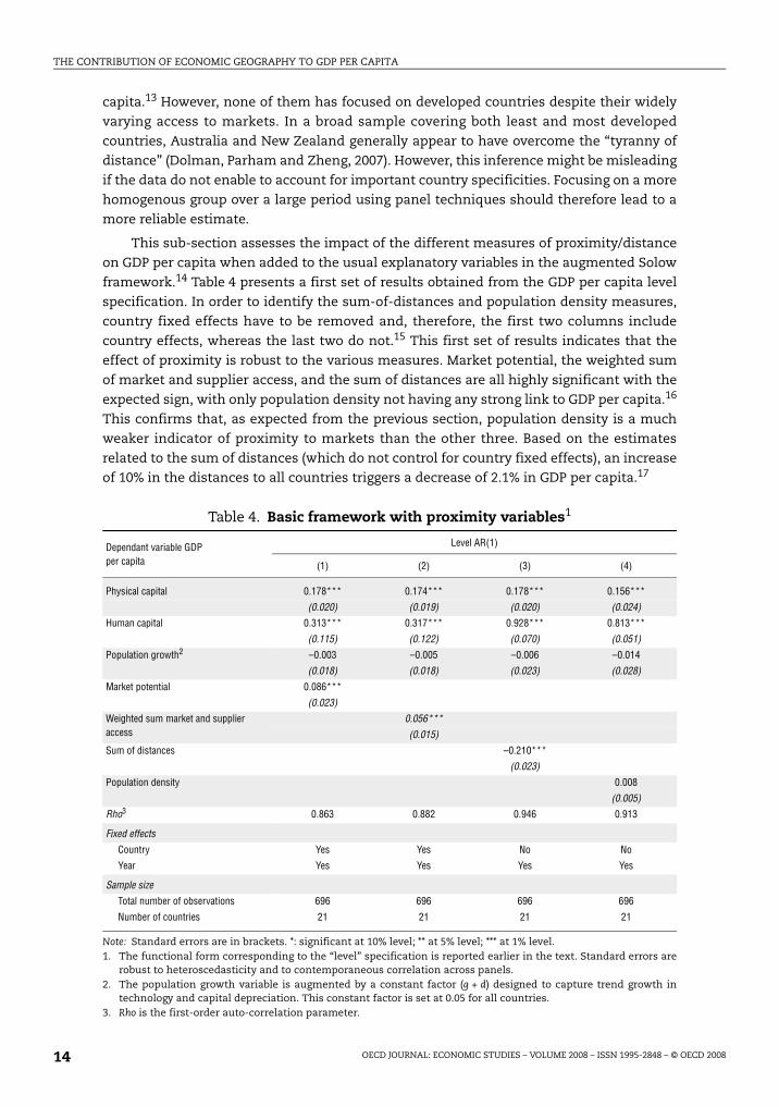
This sub-section assesses the impact of the different measures of proximity/distance
on GDP per capita when added to the usual explanatory variables in the augmented Solow
framework.14 Table 4 presents a first set of results obtained from the GDP per capita level
specification. In order to identify the sum-of-distances and population density measures,
country fixed effects have to be removed and, therefore, the first two columns include
country effects, whereas the last two do not.15 This first set of results indicates that the
effect of proximity is robust to the various measures. Market potential, the weighted sum
of market and supplier access, and the sum of distances are all highly significant with the
expected sign, with only population density not having any strong link to GDP per capita.16
This confirms that, as expected from the previous section, population density is a much
weaker indicator of proximity to markets than the other three. Based on the estimates
related to the sum of distances (which do not control for country fixed effects), an increase
of 10% in the distances to all countries triggers a decrease of 2.1% in GDP per capita.17
Table 4. Basic framework with proximity variables1
Dependant variable GDP per capita
Level AR(1)
(1) (2) (3) (4)
Physical capital 0.178*** 0.174*** 0.178*** 0.156***
(0.020) (0.019) (0.020) (0.024)
Human capital 0.313*** 0.317*** 0.928*** 0.813***
(0.115) (0.122) (0.070) (0.051)
Population growth2 –0.003 –0.005 –0.006 –0.014
(0.018) (0.018) (0.023) (0.028)
Market potential 0.086***
(0.023)
Weighted sum market and supplier access
0.056***
(0.015)
Sum of distances –0.210***
(0.023)
Population density 0.008
(0.005)
Rho3 0.863 0.882 0.946 0.913
Fixed effects
Country Yes Yes No No
Year Yes Yes Yes Yes
Sample size
Total number of observations 696 696 696 696
Number of countries 21 21 21 21
Note: Standard errors are in brackets. *: significant at 10% level; ** at 5% level; *** at 1% level.1. The functional form corresponding to the “level” specification is reported earlier in the text. Standard errors are
robust to heteroscedasticity and to contemporaneous correlation across panels.2. The population growth variable is augmented by a constant factor (g + d) designed to capture trend growth in
technology and capital depreciation. This constant factor is set at 0.05 for all countries.3. Rho is the first-order auto-correlation parameter.
OECD JOURNAL: ECONOMIC STUDIES – VOLUME 2008 – ISSN 1995-2848 – © OECD 200814
THE CONTRIBUTION OF ECONOMIC GEOGRAPHY TO GDP PER CAPITA
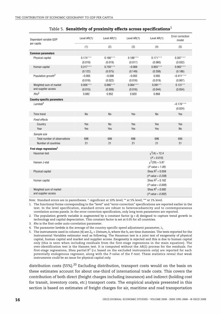
In order to test the robustness of the proximity effects across specifications, the
following results focus on the indicator that rests more firmly on sound theoretical
grounds, i.e. market and supplier access. The first three columns of Table 5 add the
weighted sum of market and supplier access to the specifications shown in columns 1 to 3
of Table 1, respectively. Market and supplier access is always highly significant, being
robust to the inclusion of country and year dummies, as well as country specific time
trends. Moreover, the estimate for the access variable is around 0.06-0.07 in all cases, while
the parameters for human and physical capital are mostly unchanged compared with
Table 1.18 This result suggests than the impact of centrality to markets acts on top of these
usual determinants. Also, the fact that excluding the country effects does not alter the
parameter significantly means that the access effect is identified by the variation through
time as well as across countries.
The estimated effect of access is fairly robust to the treatment of physical capital,
human capital and the access variables as being potentially endogenous (column 4).19
Finally, in the last column, the error correction specification is tested using the pooled
mean group estimator. Here again, the impact of centrality seems to be orthogonal to the
other dimensions, although the level of the parameter is somewhat higher.
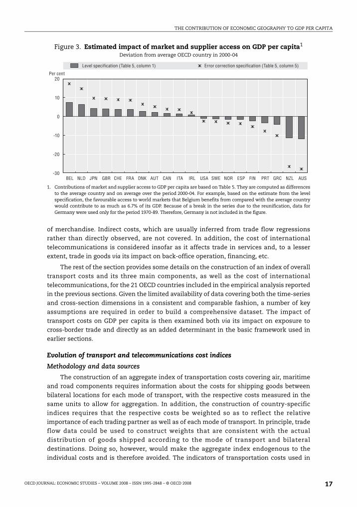
Figure 3 presents the contribution of market and supplier access to GDP per capita for
the 2000-04 period, based on the estimates in columns 1 and 5, which are representative of
the level and error-correction specifications respectively. Unsurprisingly, Australia and
New Zealand are the big losers from their geographic position. To a lesser extent, Greece,
Portugal and Finland suffer compared with the average country. The beneficiaries are core
European countries, especially Belgium and the Netherlands. As noted above, the order of
magnitude of the geography effects varies substantially depending on the specifications.
For example, market and supplier access is estimated to penalise Australia and New
Zealand by around 11% of GDP in the level specification. The effect would be almost three
times as large based on the error-correction specification, which is hardly plausible.
Conversely, Belgium and the Netherlands benefit by around 6-7% compared with the
average country in the level framework and by 16-18% in the error correction one.
Transport costsIn this section, the influence of proximity to large markets on GDP per capita is
examined through the working of a direct channel: transportation costs. The cost of
transporting goods is obviously closely linked to distance. However, shifts in modes of
transport, technological improvements in long-distance shipping and changes in fuel costs
have influenced the relationship between geographic distance and economic distance. To
some extent, the impact of transport costs was implicitly captured in the measures of
market and supplier access derived in the previous section. Nevertheless, the development
of indicators of transport costs allows for assessing directly their impact on trade and GDP
per capita, separately from other factors affecting market access, such as variations in the
degree of openness to trade across various foreign markets as well as over time.
Transport costs constitute only one source of total trade costs, albeit an important one.
According to recent estimates, broadly defined trade costs of “representative” goods
expressed in ad valorem tax-equivalent terms can be as high as 170% in industrialised
countries (Anderson and van Wincoop, 2004) with transport costs amounting to 21%, the
rest being accounted for by border-related trade barriers (44%) and retail and wholesale
OECD JOURNAL: ECONOMIC STUDIES – VOLUME 2008 – ISSN 1995-2848 – © OECD 2008 15
THE CONTRIBUTION OF ECONOMIC GEOGRAPHY TO GDP PER CAPITA
distribution costs (55%).20 Excluding distribution, transport costs would on the basis on
these estimates account for about one-third of international trade costs. This covers the
contribution of both direct (freight charges including insurance) and indirect (holding cost
for transit, inventory costs, etc.) transport costs. The empirical analysis presented in this
section is based on estimates of freight charges for air, maritime and road transportation
Table 5. Sensitivity of proximity effects across specifications1
Dependant variable GDP per capita
Level AR(1) Level AR(1) Level AR(1) Level AR(1)Error correction
model
(1) (2) (3) (4) (5)
Common parameters
Physical capital 0.174*** 0.166*** 0.188*** 0.171*** 0.307***
(0.019) (0.019) (0.017) (0.060) (0.032)
Human capital 0.317*** 0.750*** –0.069 0.855*** 0.902***
(0.122) (0.075) (0.149) (0.208) (0.186)
Population growth2 –0.005 –0.008 –0.002 0.005 –0.411***
(0.018) (0.022) (0.018) (0.019) (0.067)
Weighted sum of market and supplier access
0.056*** 0.066*** 0.064*** 0.091** 0.131**
(0.015) (0.009) (0.016) (0.044) (0.054)
Rho3 0.882 0.952 0.820 0.868
Country-specific parameters
Lambda4 –0.176***
(0.024)
Time trend No No Yes No Yes
Fixed effects
Country Yes No Yes Yes Yes
Year Yes Yes Yes Yes No
Sample size
Total number of observations 696 696 696 696 695
Number of countries 21 21 21 21 21
First stage regressions5
Hausman test 2(4) = 12.4
(P = 0.015)
Hansen J-stat 2(29) = 5.87
(P value = 1.00)
Physical capital Shea R2 = 0.059
(P value = 0.238)
Human capital Shea R2 = 0.182
(P value = 0.000)
Weighted sum of market and supplier access
Shea R2 = 0.092
(P value = 0.002)
Note: Standard errors are in parentheses. *: significant at 10% level; ** at 5% level; *** at 1% level.1. The functional forms corresponding to the “level” and “error-correction” specifications are reported earlier in the
text. In the level specification, standard errors are robust to heteroscedasticity and to contemporaneouscorrelation across panels. In the error-correction specification, only long term parameters are reported.
2. The population growth variable is augmented by a constant factor (g + d) designed to capture trend growth intechnology and capital depreciation. This constant factor is set at 0.05 for all countries.
3. Rho is the first-order auto-correlation parameter.4. The parameter lambda is the average of the country-specific speed adjustment parameter, i.
5. The instruments used in column (4) are Zit = Distsumi.ht where the ht are time dummies. The tests reported for theInstrumental Variables estimator read as following. The Hausman test is a joint test of exogeneity of physicalcapital, human capital and market and supplier access. Exogeneity is rejected and this is due to human capitalonly (this is seen when including residuals from the first-stage regressions in the main equation). Theover-identification test is the Hansen test. It is computed without the AR(1) process for the residuals. Forfirst-stage regressions, Shea partial R2 (i.e. based on the excluded instruments only) are reported for eachpotentially endogenous regressor, along with the P-value of the F-test. These statistics reveal that weakinstruments could be an issue for physical capital only.
OECD JOURNAL: ECONOMIC STUDIES – VOLUME 2008 – ISSN 1995-2848 – © OECD 200816
THE CONTRIBUTION OF ECONOMIC GEOGRAPHY TO GDP PER CAPITA
of merchandise. Indirect costs, which are usually inferred from trade flow regressions
rather than directly observed, are not covered. In addition, the cost of international
telecommunications is considered insofar as it affects trade in services and, to a lesser
extent, trade in goods via its impact on back-office operation, financing, etc.
The rest of the section provides some details on the construction of an index of overall
transport costs and its three main components, as well as the cost of international
telecommunications, for the 21 OECD countries included in the empirical analysis reported
in the previous sections. Given the limited availability of data covering both the time-series
and cross-section dimensions in a consistent and comparable fashion, a number of key
assumptions are required in order to build a comprehensive dataset. The impact of
transport costs on GDP per capita is then examined both via its impact on exposure to
cross-border trade and directly as an added determinant in the basic framework used in
earlier sections.
Evolution of transport and telecommunications cost indices
Methodology and data sources
The construction of an aggregate index of transportation costs covering air, maritime
and road components requires information about the costs for shipping goods between
bilateral locations for each mode of transport, with the respective costs measured in the
same units to allow for aggregation. In addition, the construction of country-specific
indices requires that the respective costs be weighted so as to reflect the relative
importance of each trading partner as well as of each mode of transport. In principle, trade
flow data could be used to construct weights that are consistent with the actual
distribution of goods shipped according to the mode of transport and bilateral
destinations. Doing so, however, would make the aggregate index endogenous to the
individual costs and is therefore avoided. The indicators of transportation costs used in
Figure 3. Estimated impact of market and supplier access on GDP per capita1
Deviation from average OECD country in 2000-04
1. Contributions of market and supplier access to GDP per capita are based on Table 5. They are computed as differencesto the average country and on average over the period 2000-04. For example, based on the estimate from the levelspecification, the favourable access to world markets that Belgium benefits from compared with the average countrywould contribute to as much as 6.7% of its GDP. Because of a break in the series due to the reunification, data forGermany were used only for the period 1970-89. Therefore, Germany is not included in the figure.
BEL NLD GBR FRACHE DNKJPN AUT ITACAN IRL NORSWE ESPUSA FIN PRT GRC AUSNZL
20
10
0
-10
-20
-30
Per cent
Level specification (Table 5, column 1) Error correction specification (Table 5, column 5)
OECD JOURNAL: ECONOMIC STUDIES – VOLUME 2008 – ISSN 1995-2848 – © OECD 2008 17
THE CONTRIBUTION OF ECONOMIC GEOGRAPHY TO GDP PER CAPITA
this paper are taken directly from Golub and Tomasik (2008), which provides details
regarding raw data availability, sources, assumptions made and results. The main features
can be summarised as follows:
● The basic cost of each mode of transportation between any two locations is measured in
US dollars per kilogramme shipped, and the cost of maritime shipping is assumed to be
the same for countries within a broad region (e.g. for all EU countries vis-à-vis other
broad regions).
● For each country, the costs of shipping goods to each bilateral destination are aggregated
on the basis of GDP weights of partner countries (including a country’s own GDP), as was
the case for the indicator of market potential discussed in the previous section. The
main reason for preferring GDP weights as opposed to actual trade weights is to avoid
the endogeneity of trade patterns with respect to trade costs.
● The relative importance of each mode of transport in moving goods across locations is
based on a mixture of assumptions and hard data that are available for a few countries.
The key assumption made in this context is that all trade between “neighbours” is
assumed to take place via road transportation.
● The nominal aggregate index of transport cost, expressed in dollars per kilogramme, is
deflated using either the US GDP deflator or the US price index of manufacturing goods.
Results
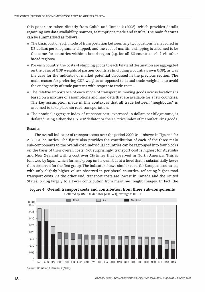
The overall indicator of transport costs over the period 2000-04 is shown in Figure 4 for
21 OECD countries. The figure also provides the contribution of each of the three main
sub-components to the overall cost. Individual countries can be regrouped into four blocks
on the basis of their overall costs. Not surprisingly, transport cost is highest for Australia
and New Zealand with a cost over 2½ times that observed in North America. This is
followed by Japan which forms a group on its own, but at a level that is substantially lower
than observed for the first group. The indicator shows similar costs for European countries,
with only slightly higher values observed in peripheral countries, reflecting higher road
transport costs. At the other end, transport costs are lowest in Canada and the United
States, owing largely to a lower contribution from maritime freight charges. In fact, the
Figure 4. Overall transport costs and contribution from three sub-componentsDeflated by US GDP deflator (2000 = 1), average 2000-04
Source: Golub and Tomasik (2008).
BELNLDFRA CHEDNKJPN AUTITA CANIRLNOR SWE GBRESP USADEUFINPRTGRCAUSNZL
0.40
0.35
0.30
0.25
0.20
0.15
0.10
0.05
0
($/kg) Road Air Maritime
OECD JOURNAL: ECONOMIC STUDIES – VOLUME 2008 – ISSN 1995-2848 – © OECD 200818
THE CONTRIBUTION OF ECONOMIC GEOGRAPHY TO GDP PER CAPITA
maritime component accounts for the largest portion of the variation in the overall costs
across the four groups of countries.
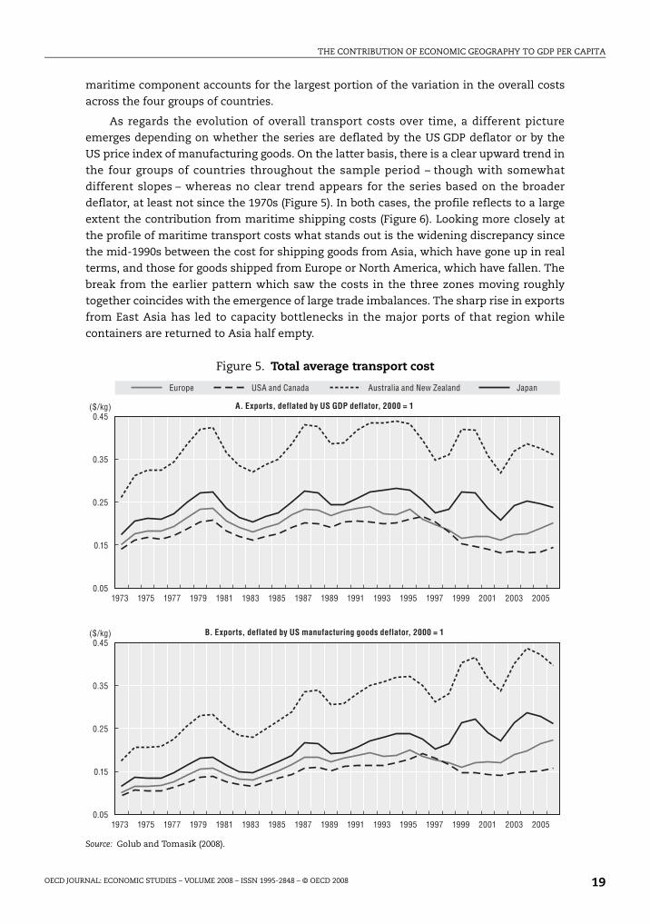
As regards the evolution of overall transport costs over time, a different picture
emerges depending on whether the series are deflated by the US GDP deflator or by the
US price index of manufacturing goods. On the latter basis, there is a clear upward trend in
the four groups of countries throughout the sample period – though with somewhat
different slopes – whereas no clear trend appears for the series based on the broader
deflator, at least not since the 1970s (Figure 5). In both cases, the profile reflects to a large
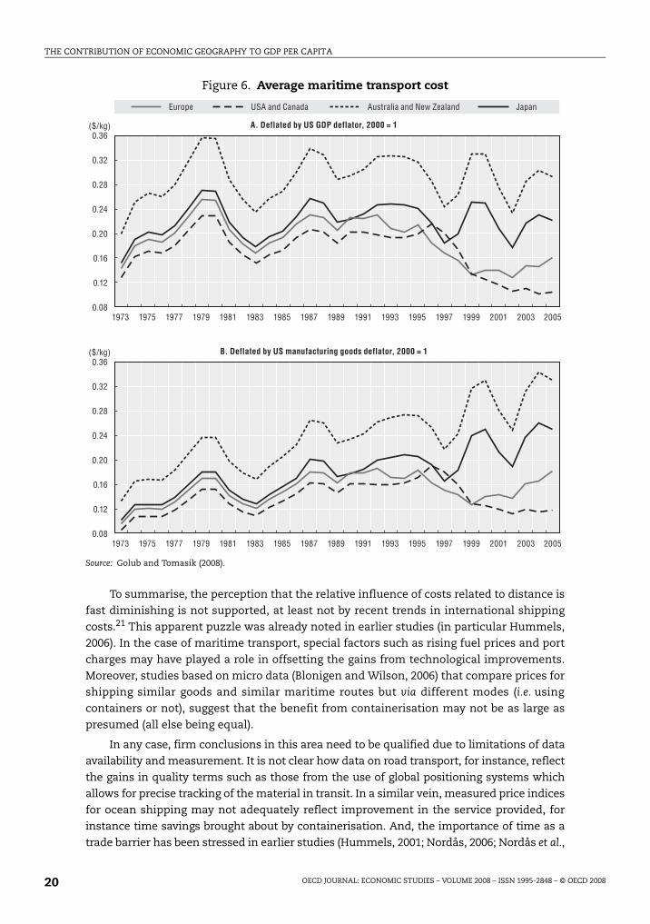
extent the contribution from maritime shipping costs (Figure 6). Looking more closely at
the profile of maritime transport costs what stands out is the widening discrepancy since
the mid-1990s between the cost for shipping goods from Asia, which have gone up in real
terms, and those for goods shipped from Europe or North America, which have fallen. The
break from the earlier pattern which saw the costs in the three zones moving roughly
together coincides with the emergence of large trade imbalances. The sharp rise in exports
from East Asia has led to capacity bottlenecks in the major ports of that region while
containers are returned to Asia half empty.
Figure 5. Total average transport cost
Source: Golub and Tomasik (2008).
0.45
0.35
0.25
0.15
0.05
($/kg)
1973 1975 1977 1979 1981 1983 1985 1987 1989 1991 1993 1995 1997 1999 2001 2003 2005
0.45
0.35
0.25
0.15
0.05
($/kg)
1973 1975 1977 1979 1981 1983 1985 1987 1989 1991 1993 1995 1997 1999 2001 2003 2005
A. Exports, deflated by US GDP deflator, 2000 = 1
B. Exports, deflated by US manufacturing goods deflator, 2000 = 1
Europe USA and Canada Australia and New Zealand Japan
OECD JOURNAL: ECONOMIC STUDIES – VOLUME 2008 – ISSN 1995-2848 – © OECD 2008 19
THE CONTRIBUTION OF ECONOMIC GEOGRAPHY TO GDP PER CAPITA
To summarise, the perception that the relative influence of costs related to distance is
fast diminishing is not supported, at least not by recent trends in international shipping
costs.21 This apparent puzzle was already noted in earlier studies (in particular Hummels,
2006). In the case of maritime transport, special factors such as rising fuel prices and port
charges may have played a role in offsetting the gains from technological improvements.
Moreover, studies based on micro data (Blonigen and Wilson, 2006) that compare prices for
shipping similar goods and similar maritime routes but via different modes (i.e. using
containers or not), suggest that the benefit from containerisation may not be as large as
presumed (all else being equal).
In any case, firm conclusions in this area need to be qualified due to limitations of data
availability and measurement. It is not clear how data on road transport, for instance, reflect
the gains in quality terms such as those from the use of global positioning systems which
allows for precise tracking of the material in transit. In a similar vein, measured price indices
for ocean shipping may not adequately reflect improvement in the service provided, for
instance time savings brought about by containerisation. And, the importance of time as a
trade barrier has been stressed in earlier studies (Hummels, 2001; Nordås, 2006; Nordås et al.,
Figure 6. Average maritime transport cost
Source: Golub and Tomasik (2008).
0.36
0.32
0.28
0.24
0.20
0.16
0.12
0.08
($/kg)
1973 1975 1977 1979 1981 1983 1985 1987 1989 1991 1993 1995 1997 1999 2001 2003 2005
0.36
0.32
0.28
0.24
0.20
0.16
0.12
0.08
($/kg)
1973 1975 1977 1979 1981 1983 1985 1987 1989 1991 1993 1995 1997 1999 2001 2003 2005
A. Deflated by US GDP deflator, 2000 = 1
B. Deflated by US manufacturing goods deflator, 2000 = 1
Europe USA and Canada Australia and New Zealand Japan
OECD JOURNAL: ECONOMIC STUDIES – VOLUME 2008 – ISSN 1995-2848 – © OECD 200820
THE CONTRIBUTION OF ECONOMIC GEOGRAPHY TO GDP PER CAPITA
2006). More generally, all transportation modes have benefited from progress in information
and communication technology as well as from a better integration via intermodal systems.
Taken at face value, the absence of a decline in the weight-based measures of real cost of
transport (i.e. nominal costs deflated by the manufacturing price index) suggests that there
may have been less technological progress in transportation than in manufacturing.
However, due to innovations outside the transport sector, the composition of traded goods
has changed significantly over the past decades, and many valuable goods are now relatively
light, e.g. electronic chips. Consequently, transport costs may well have fallen relative to the
value of transported goods.22
One area where the presumed death of distance does not seem to be at all exaggerated
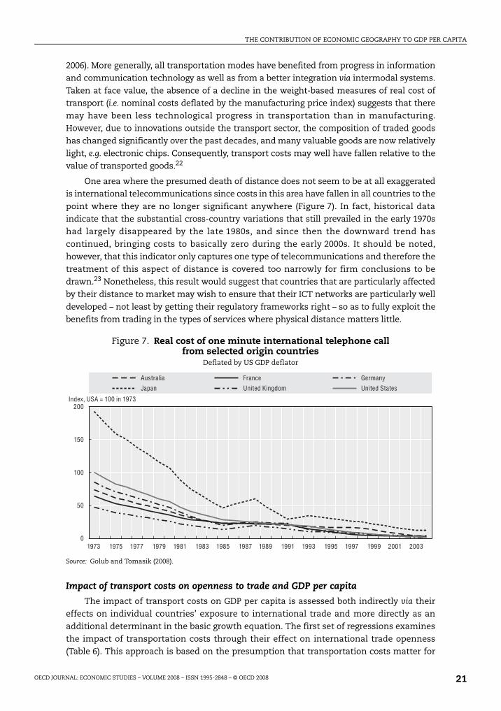
is international telecommunications since costs in this area have fallen in all countries to the
point where they are no longer significant anywhere (Figure 7). In fact, historical data
indicate that the substantial cross-country variations that still prevailed in the early 1970s
had largely disappeared by the late 1980s, and since then the downward trend has
continued, bringing costs to basically zero during the early 2000s. It should be noted,
however, that this indicator only captures one type of telecommunications and therefore the
treatment of this aspect of distance is covered too narrowly for firm conclusions to be
drawn.23 Nonetheless, this result would suggest that countries that are particularly affected
by their distance to market may wish to ensure that their ICT networks are particularly well
developed – not least by getting their regulatory frameworks right – so as to fully exploit the
benefits from trading in the types of services where physical distance matters little.
Impact of transport costs on openness to trade and GDP per capita
The impact of transport costs on GDP per capita is assessed both indirectly via their
effects on individual countries’ exposure to international trade and more directly as an
additional determinant in the basic growth equation. The first set of regressions examines
the impact of transportation costs through their effect on international trade openness
(Table 6). This approach is based on the presumption that transportation costs matter for
Figure 7. Real cost of one minute international telephone call from selected origin countries
Deflated by US GDP deflator
Source: Golub and Tomasik (2008).
200
150
100
50
01973 1975 1977 1979 1981 1983 1985 1987 1989 1991 1993 1995 1997 1999 2001 2003
Index, USA = 100 in 1973
Australia France Germany
Japan United Kingdom United States
OECD JOURNAL: ECONOMIC STUDIES – VOLUME 2008 – ISSN 1995-2848 – © OECD 2008 21
THE CONTRIBUTION OF ECONOMIC GEOGRAPHY TO GDP PER CAPITA
GDP per capita only insofar as they matter for openness and that trade contributes to GDP.
In order to assess the contribution of international trade to GDP per capita, a measure of
exposure to international trade (trade openness) is first added as a determinant in the
augmented-Solow model.24
Table 6. Basic framework with openness to trade1
Costs of transport and international communications used as an instrument for trade openness
Dependant variable GDP per capita
Level AR(1) Level AR(1) Level AR(1) Level AR(1) Level AR(1) Level AR(1)
IV IV IV
(1) (2) (3) (4) (5) (6)
Physical capital 0.175*** 0.171*** 0.164*** 0.218*** 0.208*** 0.196***
(0.020) (0.022) (0.023) (0.030) (0.021) (0.022)
Human capital 0.234* –0.273 0.740*** 0.724*** 0.210* 0.221**
(0.122) (0.324) (0.058) (0.068) (0.112) (0.112)
Population growth2 –0.016 –0.018 –0.038 –0.033 –0.028 –0.044*
(0.023) (0.025) (0.031) (0.029) (0.025) (0.026)
Trade openness 0.035* 0.029 0.048*** 0.107*** 0.068*** 0.106***
(0.020) (0.061) (0.017) (0.040) (0.020) (0.039)
Rho3 0.886 0.890 0.941 0.954 0.844 0.855
Time trend No No No No Yes Yes
Fixed effects
Country Yes Yes No No Yes Yes
Year Yes Yes Yes Yes No No
Sample size
Total number of observations 633 633 633 633 633 633
Number of countries 21 21 21 21 21 21
First stage regressions for the Trade openness variable4
Excluded instruments
Overall transport costs –0.473** –0.683*** –0.144**
(0.233) (0.065) (0.062)
Costs of international communications
0.023 –0.148*** –0.009
(0.024) (0.030) (0.027)
Sum of distances (average through time)
–0.018*** –0.004** –0.027***
(0.004) (0.002) (0.002)
Statistical tests
Hausman test ?2(1) = 2.76 ?2(1) = 3.57 ?2(1) = 5.10
(P = 0.096) (P = 0.059) (P = 0.024)
Hansen J-stat ?2(31) = 23.8 ?2(31) = 10.3 ?2(31) = 31.2
(P value = 0.820) (P value = 1.000) (P value = 0.458)
Partial R2 Shea R2 = 0.062 Shea R2 = 0.152 Shea R1 = 0.190
(P value = 0.917) (P value = 0.000) (P value = 0.000)
Note: Standard errors are in parentheses. *: significant at 10% level; ** at 5% level; *** at 1% level.1. The functional form corresponding to the “level” specification is reported earlier in the text. Standard errors are
robust to heteroscedasticity and to contemporaneous correlation across panels.2. The population growth variable is augmented by a constant factor (g + d) designed to capture trend growth in
technology and capital depreciation. This constant factor is set at 0.05 for all countries.3. rho is the first-order auto-correlation parameter.4. The instruments used in columns 2, 4 and 6 are overall transport costs, costs of international communications
and Zit = Distsumi.ht where the ht are time dummies. The tests reported for the Instrumental Variables estimatorread as following. The Hausman test is a test of exogeneity of the trade variable. The over-identification test is theHansen test. It is computed without the AR(1) process for the residuals. For first-stage regressions, Shea partial R2
(i.e. based on the excluded instruments only) is reported for the potentially endogenous regressor, along with theP-value of the F-test.
OECD JOURNAL: ECONOMIC STUDIES – VOLUME 2008 – ISSN 1995-2848 – © OECD 200822
THE CONTRIBUTION OF ECONOMIC GEOGRAPHY TO GDP PER CAPITA
The results appear in columns 1, 3 and 5 of Table 6, where the specifications vary only
according to the combination of fixed-effects and/or time trend included. The coefficient
on trade openness is positive and significant in all three cases – albeit only at the 10% level
in the first case – and varies from 0.035 when both year and country fixed-effects are
included (column 1) to twice that size when a time trend is included instead of year
fixed-effects (column 5). The coefficients on the other variables do not vary much across
specifications, except in the case of human capital, where the coefficient shows the same
sensitivity to the treatment of fixed effects as reported in previous sections. A comparison
of Table 6 with the first three columns of Table 1 also shows that adding the trade variable
does not have much impact on the parameter values of physical and human capital.
Taken at face value, these results provide evidence that greater openness to trade
leads to higher GDP per capita. However, it has long been recognised that given the
uncertainties as regards the direction of causality, the introduction of trade as an
additional determinant in the Solow model cannot be used as conclusive evidence of a
positive influence on GDP per capita, regardless of the apparent size and statistical
significance of the estimated parameter.
To address the endogeneity problem, an instrumental variable (IV) procedure is
adopted, allowing for the indicator of overall transport costs and the cost of international
telecommunications to be used as instruments for the measure of openness to
international trade in the augmented Solow model. The sum of distance, defined in the
previous section, is also used as an instrument.25 The procedure is similar to that used in
the third section and the results are reported in columns 2, 4 and 6 of Table 6. The
estimated effect of (instrumented) trade openness on GDP per capita (second stage
reported in the top panel) is significant in two of the three specifications (columns 4 and 6),
and the estimated coefficient is in these cases higher than when actual trade openness is
used (columns 3 and 5). However, this result no longer holds if one controls for both
country and year fixed effects, where the coefficient on trade openness is not significant
(column 2).26 As for the results from the first-stage regression (bottom panel), they show
that overall transport costs have a significant (negative) impact on trade openness in all
three IV specifications, although with large variations in the parameter estimates.
Overall, these results indicate that transportation costs contribute to reduce the
exposure to international trade and that in turn the latter appears to have a significant
impact on GDP per capita. In contrast, the effect of international telecommunications on
trade openness is significant only when country fixed effects are not included, and
therefore the evidence is much weaker. The results from the IV procedure provides some
evidence that trade openness may have a causal influence on GDP per capita, consistent
with earlier findings (e.g. Frankel and Romer, 1999).
Against this background, the contribution of transport costs to GDP per capita is
reported in Figure 8. In order to provide a range of estimates, the contribution is calculated
on the basis of coefficients obtained from two specifications based on Table 6 (columns 4
and 6, respectively). On this basis, high transport costs relative to the OECD average are
found to reduce GDP per capita by between 1.0% and 4.5% in Australia and New Zealand,
where the effect is largest. At the other end, the lower transport costs for Canada and the
United States contribute to raise GDP per capita by between 0.5% and 2.5%.
OECD JOURNAL: ECONOMIC STUDIES – VOLUME 2008 – ISSN 1995-2848 – © OECD 2008 23
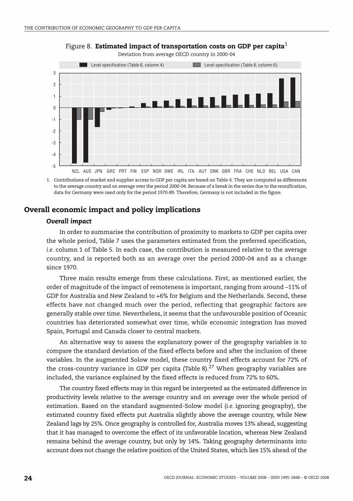
THE CONTRIBUTION OF ECONOMIC GEOGRAPHY TO GDP PER CAPITA
Overall economic impact and policy implications
Overall impact
In order to summarise the contribution of proximity to markets to GDP per capita over
the whole period, Table 7 uses the parameters estimated from the preferred specification,
i.e. column 1 of Table 5. In each case, the contribution is measured relative to the average
country, and is reported both as an average over the period 2000-04 and as a change
since 1970.
Three main results emerge from these calculations. First, as mentioned earlier, the
order of magnitude of the impact of remoteness is important, ranging from around –11% of
GDP for Australia and New Zealand to +6% for Belgium and the Netherlands. Second, these
effects have not changed much over the period, reflecting that geographic factors are
generally stable over time. Nevertheless, it seems that the unfavourable position of Oceanic
countries has deteriorated somewhat over time, while economic integration has moved
Spain, Portugal and Canada closer to central markets.
An alternative way to assess the explanatory power of the geography variables is to
compare the standard deviation of the fixed effects before and after the inclusion of these
variables. In the augmented Solow model, these country fixed effects account for 72% of
the cross-country variance in GDP per capita (Table 8).27 When geography variables are
included, the variance explained by the fixed effects is reduced from 72% to 60%.
The country fixed effects may in this regard be interpreted as the estimated difference in
productivity levels relative to the average country and on average over the whole period of
estimation. Based on the standard augmented-Solow model (i.e. ignoring geography), the
estimated country fixed effects put Australia slightly above the average country, while New
Zealand lags by 25%. Once geography is controlled for, Australia moves 13% ahead, suggesting
that it has managed to overcome the effect of its unfavorable location, whereas New Zealand
remains behind the average country, but only by 14%. Taking geography determinants into
account does not change the relative position of the United States, which lies 15% ahead of the
Figure 8. Estimated impact of transportation costs on GDP per capita1
Deviation from average OECD country in 2000-04
1. Contributions of market and supplier access to GDP per capita are based on Table 6. They are computed as differencesto the average country and on average over the period 2000-04. Because of a break in the series due to the reunification,data for Germany were used only for the period 1970-89. Therefore, Germany is not included in the figure.
BELNLDFRA CHEDNKJPN AUTITA CANIRLNOR SWE GBRESP USAFINPRTGRCAUSNZL
3
2
1
0
-1
-2
-3
-4
-5
Level specification (Table 6, column 4) Level specification (Table 6, column 6)
OECD JOURNAL: ECONOMIC STUDIES – VOLUME 2008 – ISSN 1995-2848 – © OECD 200824
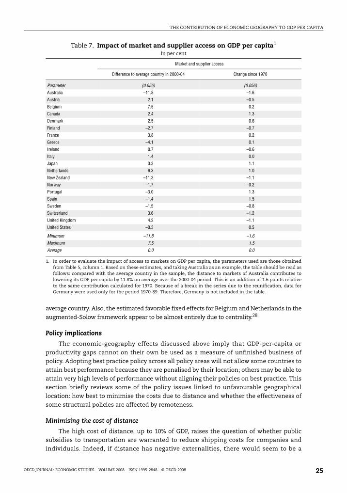
THE CONTRIBUTION OF ECONOMIC GEOGRAPHY TO GDP PER CAPITA
average country. Also, the estimated favorable fixed effects for Belgium and Netherlands in the
augmented-Solow framework appear to be almost entirely due to centrality.28
Policy implications
The economic-geography effects discussed above imply that GDP-per-capita or
productivity gaps cannot on their own be used as a measure of unfinished business of
policy. Adopting best practice policy across all policy areas will not allow some countries to
attain best performance because they are penalised by their location; others may be able to
attain very high levels of performance without aligning their policies on best practice. This
section briefly reviews some of the policy issues linked to unfavourable geographical
location: how best to minimise the costs due to distance and whether the effectiveness of
some structural policies are affected by remoteness.
Minimising the cost of distance
The high cost of distance, up to 10% of GDP, raises the question of whether public
subsidies to transportation are warranted to reduce shipping costs for companies and
individuals. Indeed, if distance has negative externalities, there would seem to be a
Table 7. Impact of market and supplier access on GDP per capita1
In per cent
Market and supplier access
Difference to average country in 2000-04 Change since 1970
Parameter (0.056) (0.056)
Australia –11.8 –1.6
Austria 2.1 –0.5
Belgium 7.5 0.2
Canada 2.4 1.3
Denmark 2.5 0.6
Finland –2.7 –0.7
France 3.8 0.2
Greece –4.1 0.1
Ireland 0.7 –0.6
Italy 1.4 0.0
Japan 3.3 1.1
Netherlands 6.3 1.0
New Zealand –11.3 –1.1
Norway –1.7 –0.2
Portugal –3.0 1.3
Spain –1.4 1.5
Sweden –1.5 –0.8
Switzerland 3.6 –1.2
United Kingdom 4.2 –1.1
United States –0.3 0.5
Minimum –11.8 –1.6
Maximum 7.5 1.5
Average 0.0 0.0
1. In order to evaluate the impact of access to markets on GDP per capita, the parameters used are those obtainedfrom Table 5, column 1. Based on these estimates, and taking Australia as an example, the table should be read asfollows: compared with the average country in the sample, the distance to markets of Australia contributes tolowering its GDP per capita by 11.8% on average over the 2000-04 period. This is an addition of 1.6 points relativeto the same contribution calculated for 1970. Because of a break in the series due to the reunification, data forGermany were used only for the period 1970-89. Therefore, Germany is not included in the table.
OECD JOURNAL: ECONOMIC STUDIES – VOLUME 2008 – ISSN 1995-2848 – © OECD 2008 25
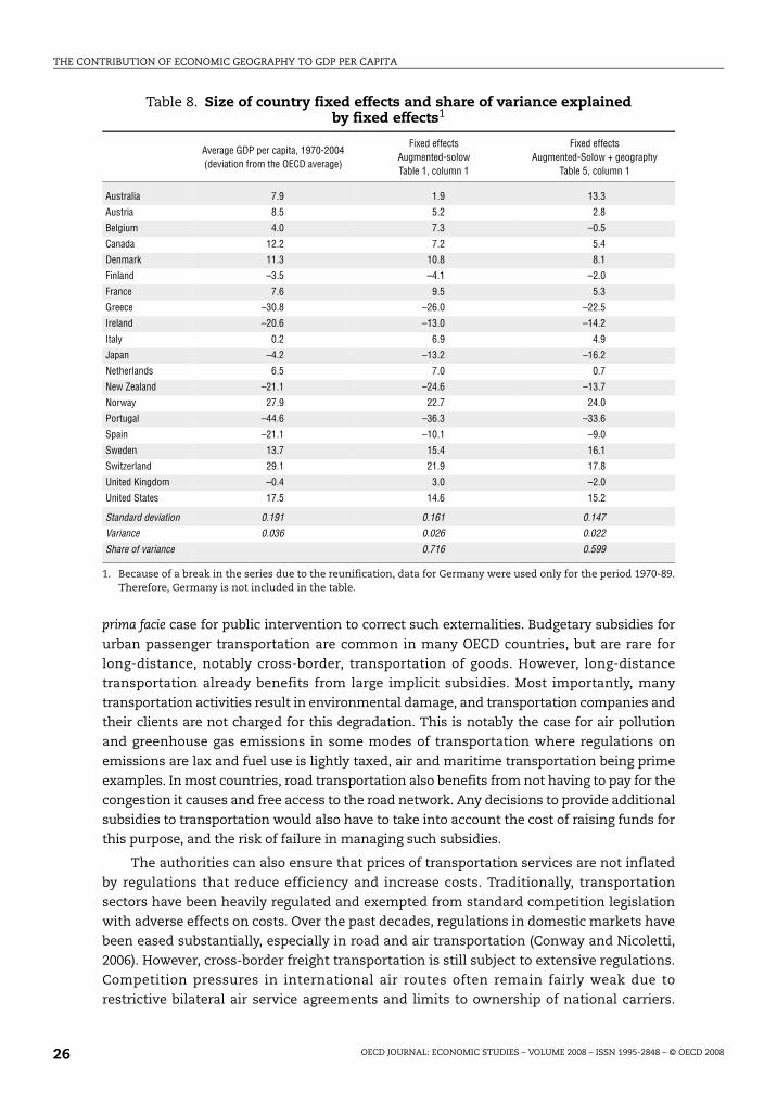
THE CONTRIBUTION OF ECONOMIC GEOGRAPHY TO GDP PER CAPITA
prima facie case for public intervention to correct such externalities. Budgetary subsidies for
urban passenger transportation are common in many OECD countries, but are rare for
long-distance, notably cross-border, transportation of goods. However, long-distance
transportation already benefits from large implicit subsidies. Most importantly, many
transportation activities result in environmental damage, and transportation companies and
their clients are not charged for this degradation. This is notably the case for air pollution
and greenhouse gas emissions in some modes of transportation where regulations on
emissions are lax and fuel use is lightly taxed, air and maritime transportation being prime
examples. In most countries, road transportation also benefits from not having to pay for the
congestion it causes and free access to the road network. Any decisions to provide additional
subsidies to transportation would also have to take into account the cost of raising funds for
this purpose, and the risk of failure in managing such subsidies.
The authorities can also ensure that prices of transportation services are not inflated
by regulations that reduce efficiency and increase costs. Traditionally, transportation
sectors have been heavily regulated and exempted from standard competition legislation
with adverse effects on costs. Over the past decades, regulations in domestic markets have
been eased substantially, especially in road and air transportation (Conway and Nicoletti,
2006). However, cross-border freight transportation is still subject to extensive regulations.
Competition pressures in international air routes often remain fairly weak due to
restrictive bilateral air service agreements and limits to ownership of national carriers.
Table 8. Size of country fixed effects and share of variance explained by fixed effects1
Average GDP per capita, 1970-2004 (deviation from the OECD average)
Fixed effects Augmented-solow Table 1, column 1
Fixed effects Augmented-Solow + geography
Table 5, column 1
Australia 7.9 1.9 13.3
Austria 8.5 5.2 2.8
Belgium 4.0 7.3 –0.5
Canada 12.2 7.2 5.4
Denmark 11.3 10.8 8.1
Finland –3.5 –4.1 –2.0
France 7.6 9.5 5.3
Greece –30.8 –26.0 –22.5
Ireland –20.6 –13.0 –14.2
Italy 0.2 6.9 4.9
Japan –4.2 –13.2 –16.2
Netherlands 6.5 7.0 0.7
New Zealand –21.1 –24.6 –13.7
Norway 27.9 22.7 24.0
Portugal –44.6 –36.3 –33.6
Spain –21.1 –10.1 –9.0
Sweden 13.7 15.4 16.1
Switzerland 29.1 21.9 17.8
United Kingdom –0.4 3.0 –2.0
United States 17.5 14.6 15.2
Standard deviation 0.191 0.161 0.147
Variance 0.036 0.026 0.022
Share of variance 0.716 0.599
1. Because of a break in the series due to the reunification, data for Germany were used only for the period 1970-89.Therefore, Germany is not included in the table.
OECD JOURNAL: ECONOMIC STUDIES – VOLUME 2008 – ISSN 1995-2848 – © OECD 200826
THE CONTRIBUTION OF ECONOMIC GEOGRAPHY TO GDP PER CAPITA
Road transportation on many international routes is hampered by lack of “cabotage” rights.
And international scheduled maritime freight services are still operated as price-setting
cartels on many key routes, reflecting that this activity is exempted from national
competition legislation in many OECD countries. Moreover, port efficiency varies widely
across countries and affects shipping costs significantly, in part due to regulatory
restrictions hampering competition in port services (Clark, Dollar and Micco, 2004).
Distance and the effectiveness of structural policies
Remoteness can in principle influence the effectiveness of some structural policy
measures, with implications for policy choices. A possible interaction between policy and
distance is that a given policy change to strengthen competition in domestic product
markets may have a weaker influence in remote countries than in countries close to large
markets, even if such reforms are arguably more needed in the former group of countries
as they have limited alternatives to enhance competition. In countries at a large distance
from world markets, there may not be room for many competitors in some sectors if the
efficient scale of operation is close to the size of the market. In such circumstances the
lifting of statutory entry barriers may not stimulate entry, as the size of the market will
de facto restrict the number of competitors. On the other hand, if legal entry barriers are the
binding constraint on entry as seems more likely in countries close to world markets, then
lowering such barriers should stimulate competition. Notwithstanding the intuitive appeal
of such arguments, no evidence that distance significantly interacts with a measure of
competition-restraining regulations could be found on the basis of an admittedly crude
empirical investigation. Indeed, the first three columns of Table 9 show, first, that both
product market regulation and access to markets remain significant when they are jointly
included in the basic equation and, second, that the interaction between regulation and
proximity is not significant.
Another area where the effectiveness of policies might be expected to vary depending
on distance is R&D spending.29 Such activity is likely to involve significant fixed costs and
thus be subject to economies of scale. With distance limiting the size of the market, the
unit cost of innovation can be expected to be higher in remote countries than in countries
close to large markets where fixed costs can be spread more widely. Another related
channel is the reduced incentives for large multinational firms to establish a commercial
presence in remote markets, due to the limited development possibilities. Since
multinational firms are the main carriers of innovation to other markets, the impact of
domestic R&D spending on growth in foreign markets is limited by their absence in smaller
remote markets. Hence, a given increase in public and/or private R&D spending is likely to
have a greater leverage and therefore a greater GDP-per-capita impact in countries with
short distance to markets than in more remote countries. Furthermore, insofar as the
effectiveness of public and/or private R&D can be influenced by the strength of industry
and science linkages or by close interactions between researchers from various
institutions, the impact of R&D on GDP per capita may vary according to the extent of
urban concentration within a country.
These possibilities are examined via the introduction in the estimated equation of two
interaction terms, one between private R&D and distance and the other between private
R&D and the share of the country population living in cities of more than 1 million
inhabitants (urban concentration). A measure of R&D intensity (business R&D as a ratio of
GDP) is first introduced as an additional determinant in the augmented Solow model
OECD JOURNAL: ECONOMIC STUDIES – VOLUME 2008 – ISSN 1995-2848 – © OECD 2008 27
THE CONTRIBUTION OF ECONOMIC GEOGRAPHY TO GDP PER CAPITA
(column 4), where it comes out significant (although at the 10% confidence level). The
specification with the two interaction terms is then shown in column 5 of Table 9, where
the results suggest that the effectiveness of private R&D intensity is significantly
influenced by the degree of urban concentration, but not by distance to major markets.30
A third policy area where geographic factors might be important is human capital
formation. In this case, however, the relevant geographic factor is not distance to world
Table 9. Geography and the effectiveness of structural policies1
Dependant variable GDP per capita
Level AR(1) Level AR(1) Level AR(1) Level AR(1) Level AR(1) Level AR(1) Level AR(1) Level AR(1)
(1) (2) (3) (4) (5) (6) (7) (8)
Physical capital 0.209*** 0.199*** 0.199*** 0.222*** 0.213*** 0.221*** 0.218*** 0.222***
(0.021) (0.021) (0.021) (0.023) (0.023) (0.023) (0.023) (0.022)
Human capital 0.240*** 0.263*** 0.231*** 0.203** 0.223** 0.366*** 0.469*** 0.579***
(0.087) (0.086) (0.088) (0.090) (0.095) (0.115) (0.118) (0.134)
Population growth2 –0.031 –0.027 –0.028 0.018 0.019 –0.009 –0.012 –0.011
(0.021) (0.021) (0.028) (0.035) (0.035) (0.022) (0.023) (0.023)
Weighted sum market and supplier access
0.054*** 0.052*** 0.041** 0.038** 0.048** 0.041**
(0.018) (0.018) (0.021) (0.019) (0.020) (0.020)
PMR3 –0.035* –0.038* –0.035*
(0.019) (0.020) (0.020)
PMR * Population density 0.007
(0.007)
PMR * Weighted sum market and supplier access
–0.003
(0.010)
Business R&D4 0.027* 0.031*
(0.015) (0.016)
Business R&D * Urban concentration
0.114**
(0.056)
Business R&D * Weighted sum market and supplier access
0.007
(0.009)
Human capital * Urban concentration5
0.927*** 1.341***
(0.193) (0.251)
Human capital * Population density6
–0.129*** –0.219***
(0.035) (0.047)
Time trend 0.017*** 0.017*** 0.017*** 0.020*** 0.020*** 0.018*** 0.017*** 0.017***
(0.001) (0.001) (0.001) (0.001) (0.001) (0.001) (0.001) (0.001)
Rho7 0.843 0.844 0.861 0.857 0.853 0.831 0.827 0.846
Fixed effects
Country Yes Yes Yes Yes Yes Yes Yes Yes
Sample size
Total number of observations 595 595 595 344 344 696 696 696
Number of countries 21 21 21 21 21 21 21 21
Note: Standard errors are in parentheses. *: significant at 10% level; ** at 5% level; *** at 1% level.1. The functional form corresponding to the “level” specification is reported earlier in the text. Standard errors are robust to
heteroscedasticity and to contemporaneous correlation across panels. All interaction variables are constructed from thedemeaned respective variables. That way, the estimated parameters on the non-interacted variables still measure theaverage effect of these variables.
2. The population growth variable is augmented by a constant factor (g + d) designed to capture trend growth in technologyand capital depreciation. This constant factor is set at 0.05 for all countries.
3. PMR is the product market regulation index which is built in a 0-6 scale. It is introduced in logs.4. Due to limitations in data, the sample for regressions involving R&D spending is substantially reduced. This is because data
on R&D are generally only available from 1981 to 2003/04, and 6 of the 21 countries do not have sufficiently long series to beincluded. Note also that private R&D is entered in the regression with one lag.
5. Urban concentration is the share of the country population living in cities of more than 1 million inhabitants.6. Population density measure is the ratio of population to surface area.7. Rho is the first-order auto-correlation parameter.
OECD JOURNAL: ECONOMIC STUDIES – VOLUME 2008 – ISSN 1995-2848 – © OECD 200828
THE CONTRIBUTION OF ECONOMIC GEOGRAPHY TO GDP PER CAPITA
markets but rather economic density, in particular the degree of agglomeration.
A hypothetical benefit of agglomeration is that there are strong knowledge spillovers
associated with proximity, whereby “tacit” or informal knowledge is transmitted via
face-to-face contact. To the extent that such kind of knowledge is related to cognitive skills
acquired during formal schooling, reforms that strengthen educational performance may
have stronger productivity raising effects in densely populated urban centres than in areas
where population density is lower. If this were to be the case, countries where the
population is concentrated in large urban areas would benefit more from educational
reforms than countries where the population settlement is more dispersed. The
preliminary empirical evidence, as reported in the last three columns of Table 9, is
inconclusive. Taking the estimates at face value, the impact of human capital on GDP per
capita seems to be strengthened by urban concentration, whereas the opposite result is
obtained when the density measure is the ratio of population to surface area.
ConclusionsThis paper examines how much of the dispersion in economic performance across
OECD countries can be accounted for by economic geography factors. More specifically, the
proximity to areas of dense economic activity has been examined. To do so, various
indicators of distance to markets and transportation costs have been added sequentially as
determinants in an augmented Solow model, which is used as a benchmark.
Three measures of distance to markets are found to have a statistically significant
effect on GDP per capita: the sum of bilateral distances, market potential and the weighted
sum of market access and supplier access. And the estimated economic impact, which
varies somewhat across specifications, is far from negligible. For instance, the lower access
to markets relative to the OECD average could contribute negatively to GDP per capita by as
much as 11% in Australia and New Zealand. Conversely, the benefit from a favourable
location could account for as much as 6-7% of GDP in the case of Belgium and the
Netherlands. The impact of transport costs on GDP per capita is also found to be
statistically significant, albeit less so in economic terms. For instance, differences in
transport costs relative to the OECD average contribute to reduce GDP per capita by
between 1.0% and 4.5% in Australia and New Zealand. At the other end, the lower transport
costs for Canada and the United States contributes to raise GDP per capita relative to the
average OECD country, but only by a small margin varying between 0.5% and. 2.5%. These
quantitatively smaller effects are consistent with transportation costs being only one
aspect of distance-related costs.
Considering the substantial estimated effect that distance/proximity to major markets
has on GDP per capita, one issue is whether there is a role for public authorities to
subsidise international transport, at least in the most remote countries, so as to partly
compensate for additional trade costs incurred. Against this, it can be argued that
transport is already subsidised in many ways, if only because transport industries only
partly bear the cost of negative externalities such as pollution and road congestion.
Moreover, subsidisation involves well-known issues of government failure. Less
controversial, public policies can also contribute to reduce the cost of transportation by
strengthening competition in transport industries, which have in the past been heavily
regulated. However, considering that since the mid-1980s domestic regulation has been
eased to some extent, at least in air and road transport, further gains in this area may come
OECD JOURNAL: ECONOMIC STUDIES – VOLUME 2008 – ISSN 1995-2848 – © OECD 2008 29
THE CONTRIBUTION OF ECONOMIC GEOGRAPHY TO GDP PER CAPITA
from reductions in regulatory barriers to cross-border freight transport, an area where less
progress has been achieved.
Insofar as distance or remoteness may affect the effectiveness of policy, another policy
issue is whether the possibility that what constitutes “best practice” in a particular area
may differ across countries. Some tentative estimates of these effects have been conducted
with respect to product market regulation, human capital and R&D spending. The
preliminary results do not provide strong evidence of an impact of remoteness on the
effectiveness of policy in these areas. However, there is some evidence that spending on
R&D and human capital might have a stronger effect on GDP per capita in countries with
higher urban concentration.
Notes
1. The implications of imposing invalid homogeneity restrictions on slope parameters in the contextof dynamic panel estimates are discussed in Lee, Pesaran and Smith (1997).
2. The reason is that the number of determinants that can be jointly estimated is limited by availabledegrees of freedom and risks of multi-collinearity. Hence, the variables can only be testedsequentially with the number of possible permutations rising exponentially with the set ofdeterminants. Sala-i-Martin et al., (2004) have proposed a bayesian method to deal with thisstandard problem in empirical growth analysis.
3. In principle, a measure of investment in human capital should be used to be consistent with thetreatment of physical capital in the basic Solow model. In practice, a proxy for the stock – averagenumber of years of schooling – is used due to the absence of an adequate measure of the flow.However, to ensure consistency with the theoretical model, the measure of stock is introducedboth in level and first-difference forms, even in the “level” specification.
4. Following a standard approach in the literature, this constant factor (g + d) is set at 0.05 for allcountries (Mankiw et al., 1992).
5. Doing so makes it close to a growth rate or error correction model specification, with constraintsimposed on the short-term dynamics (see Beck and Katz, 2004, for further details). In that sense,one minus the first-order correlation parameter can be compared with the annual speed ofconvergence.
6. For a direct comparison, see the results reported in OECD (2003), Table 2.4, second column, onpage 81.
7. In fact, the inclusion of specific trend parameters distorts the notion of convergence, since itshould then be interpreted as convergence to a different steady-state growth rate across countries(Lee, Pesaran and Smith, 1997, and Islam, 1998). It is therefore not surprising that in such case theestimated speed of convergence of around 19% per annum is higher than when parameterhomogeneity is imposed across countries.
8. The sensitivity of human capital to the treatment of the time trend in either level or error-correctionspecifications can be partly explained by the fact that it is proxied by a variable (average number ofyears of schooling) that is characterised by a very smooth upward-trend profile over time.
9. In order to minimise the number of determinants shown separately on the graph, the contributionof population growth is lumped with that of physical capital and the contribution of fixed effectscover both year and fixed effects in the top panel and country fixed effects and time trend in thelower panel.
10. The underlying assumption behind the internal distance is that a country is adisk where all suppliers are located in the center and consumers are located uniformly over thearea. An alternative measure consists in using the largest cities in each country both for externaland internal distances. This entails some differences depending on the size of the countries.However, the results in this paper proved to be robust to the choice of the distance definition.
11. When variables are compared in yearly changes over the whole panel rather than in levels, thecorrelation is still very significant, but falls to 50% and 36% between market potential, on the onehand, and market and supplier access, respectively, on the other hand.
π/3/2 ii i aread =
OECD JOURNAL: ECONOMIC STUDIES – VOLUME 2008 – ISSN 1995-2848 – © OECD 200830
THE CONTRIBUTION OF ECONOMIC GEOGRAPHY TO GDP PER CAPITA
12. In that context, the higher calculated total market potential for Canada than for the United Statesreflects the specific capital-to-capital measure of distance. Whereas the internal distance for theUnited States is 1 161 km, the capital-to-capital distance between the two countries is 737 km.Hence, this measure of distance gives the US GDP a greater weight for Canada than for the UnitedStates itself. This feature disappears when the distance measure takes into account not only thecapital but also the biggest cities in each country (see Boulhol and de Serres, 2008).
13. Redding and Venables apply their framework to a cross-section of 101 countries, while Breinlich(2007), highlighting that regional income levels in the European Union display a strongcore-periphery gradient, tests the impact of market access using a panel of European regionsover 1975-97. Head and Mayer (2007) conduct a similar exercise based on European sectoral dataover a shorter period. Concurrently, Hanson (2005) develops a model assuming labour mobility andtests it using data covering US counties. Combes and Overman (2004) present a survey of studiesreplicating Hanson’s approach for various European countries.
14. Based on a cross-section of 148 countries, an earlier study showed that proximity (marketpotential) explains a significant fraction of the income pattern even after controlling for the usualdeterminants in Solow-type regressions (Hummels, 1995).
15. As in the second section (Table 1), the human capital parameter is very sensitive to whethercountry fixed effects are included.
16. Due to the strong correlation between market and supplier access, the specific effect of eachindicator cannot be identified. However, the explanatory variable in the model is a weighted sumof the two indicators, the weights being given by structural parameters; see Boulhol and de Serres(2008) for details.
17. This would imply, for example, that the relatively large distance of Australia from world marketscompared with the United States accounts for a GDP-per-capita gap of around 12 percentage points(given the values of the sum-of-distances measure reported in Table 3, 0.21.ln(214/119) 0.12).
18. These estimates are consistent with those shown in Boulhol and de Serres (2008) based on thepure Redding and Venables model in which market and supplier access are the only determinantsof GDP per capita, once time and country fixed effects are controlled for.
19. In order to try to overcome the potential endogeneity bias, the sum of distances variable, Distsum,is an ideal instrument. Taking advantage of the panel dimension of the data, the effect of thistime-invariant instrument is allowed to vary through time. In other words, a set of instruments,Zit = distsumi.ht, are used where the ht are time dummies.
20. The overall cost is computed as 1.21 * 1.44 * 1.55 – 1 = 1.7. Border-related costs include policybarriers (tariffs and non-tariffs), information and enforcement costs, as well as costs due to the useof different currencies, rules and legal frameworks.
21. A clear downward trend in the relative price of merchandise transportation appears in the case ofair transport, but only if the series is deflated by the GDP deflator rather than the narrower indexof manufacturing goods prices.
22. According to Hummels (2007), the weight/value ratio of traded goods has fallen especially for theUnited States, since the early 1990s: $1 (in real terms) of traded merchandise weighs much lesstoday than in the 1970s. Hummels reports that the real value of trade grew 1.5% per year fasterthan its weight since 1973. Because the measures above refer to the costs in dollar per kg, and havebeen constructed on the basis of an unchanged weight/value ratio over time, they underestimaterelative the decline in ad valorem transport costs.
23. For telecommunications, an alternative approach would have been to look at measures of“distance” such as, for instance, the total outbound international network capacity in eachcountry, either in absolute or per inhabitant. Unfortunately, such measures are typically notavailable before the 1990s.
24. Trade openness is measured as the average of export and import intensities (i.e. as a ratio of GDP)and is adjusted for country size. The adjustment is made by regressing the raw trade opennessvariable on population size and by taking the estimated residual from that panel regression as themeasure of trade exposure that is included as an additional determinant in the augmented Solowspecification.
25. Even though the variable does not have a time-series dimension, its estimated impact is allowedto vary over time. The value reported in the bottom panel of Table 6, is the average of all parameterestimates.
OECD JOURNAL: ECONOMIC STUDIES – VOLUME 2008 – ISSN 1995-2848 – © OECD 2008 31
THE CONTRIBUTION OF ECONOMIC GEOGRAPHY TO GDP PER CAPITA
26. The statistical tests reported at the bottom of Table 6 indicate that when both year and countryfixed-effects are included (column 2), the instruments add little information and are thereforeconsidered as weak.
27. The dispersion across countries of the average (log of) real GDP per capita over the period is 0.191,whereas the standard deviation of the country fixed effects in the estimated steady-state (Table 1,column 1) is 0.161 and (0.161/0.191)2 = 72%.
28. A similar exercise cannot be replicated concerning the impact of the transport costs variables. Thereason is that, as shown in the previous section, the effects of transport costs are robust only viatheir impact on international trade. The fixed effects obtained from a specification that includestrade openness as a determinant of GDP per capita could have been reported, but these would bemisleading as transport costs are one of the determinants of trade only.
29. R&D spending was left out from the specifications in previous sections because limitations in dataavailability would have led to a substantial reduction in sample size (from nearly 600 to around350 observations), and also because the focus of the study is on economic geographydeterminants.
30. In this specification, the ratio of R&D spending to GDP is used as a proxy for investment ininnovation. Although in absence of knowledge depreciation, a decline in the R&D intensity shouldnot lead to a fall in GDP per capita, the specification implies that a switch to a steady-statecorresponding to a lower R&D intensity would entail moving to a path with a lower GDP per capita.
Bibliography
Arnold, J., A. Bassanini and S. Scarpetta (2007), “Is it Solow or Lucas ?”, OECD Economics DepartmentWorking Papers, No. 592.
Bassanini, A. and S. Scarpetta (2001), “Does Human Capital Matter for Growth in OECD Countries?Evidence from PMG Estimates”, OECD Economics Department Working Papers, No. 282.
Beck, N. and J.N. Katz (2004), “Time Series Cross Section Issues: Dynamics, 2004”, Paper presented atthe 2004 Annual Meeting of the Society for Political Methodology, Stanford University.
Bernanke, B.S. and R.S. Gürkaynak (2001), “Is Growth Exogenous? Taking Mankiw, Romer and WeilSeriously”, NBER Macroeconomics Annual.
Blonigen, B. and W. Wilson (2006), “New Measures of Port Efficiency Using International Trade Data”,NBER Working Paper No. 12052.
Boulhol, H. and A. de Serres (2008), “Have Developed Countries Escaped the Curse of Distance?”, OECDEconomics Department Working Papers, No. 610.
Breinlich, H. (2007), “The Spatial Income Structure in the European Union – What Role for EcononomicGeography?”, Journal of Economic Geography, forthcoming.
Clark, X., D. Dollar and A. Micco (2004), “Port efficiency, Maritime Transport Costs and Bilateral Trade”,Journal of Development Economics, Vol. 75, No. 2.
Combes, P.-P. and H.G. Overman (2004), “The Spatial Distribution of Economic Activities in theEuropean Union”, in V. Henderson and J.-F. Thisse (eds.), Handbook of Urban and Regional Economics,Vol. 4, Elsevier-North Holland, Amsterdam.
Conway, P. and G. Nicoletti (2006), “Product Market Regulation in the Non-Manufacturing Sectors ofOECD Countries: Measurement and Highlights”, OECD Economics Department Working Papers,No. 530.
Dolman, B., D. Parham and S. Zheng (2007), “Can Australia Match US Productivity Performance?”,Australia Government Productivity Commission, Staff Working Paper, March.
Durlauf, S.N. and D. Quah (1999), “The New Empirics of Economic Growth”, Handbook of Macroeconomics,J.B. Taylor and M. Woodford (eds.), Vol. 1, Chapter 4.
Eaton, J. and S. Kortum (1994), “International Patenting and Technology Diffusion”, NBER Working Paper,No. 4931.
Eaton, J. and S. Kortum (1996), “Trade in Ideas: Patenting and Productivity in the OECD”, Journal ofInternational Economics, Vol. 40, No. 3-4.
Frankel, J. and D. Romer (1999), “Does Trade Cause Growth?”, American Economic Review, Vol. 84, No. 1.
OECD JOURNAL: ECONOMIC STUDIES – VOLUME 2008 – ISSN 1995-2848 – © OECD 200832
THE CONTRIBUTION OF ECONOMIC GEOGRAPHY TO GDP PER CAPITA
Golub, S.S. and B. Tomasik (2008), “Measures of International Transport Cost for OECD Countries”,OECD Economics Department Working Papers, forthcoming.
Hall, R.E. and C.I. Jones (1999), “Why Do Some Countries Produce so Much More Output per WorkerThan Others?”, Quarterly Journal of Economics, Vol. 114, No. 1.
Hanson, G.H. (2005), “Market Potential, Increasing Returns and Geographic Concentration”, Journal ofInternational Economics, Vol. 67, No. 1.
Harris, C. (1954), “The Market as a Factor in the Localisation of Industry in the United States”, Annals ofthe Association of National Geographers, Vol. 44, No. 4.
Head, K. and T. Mayer (2006), “Regional Wage and Employment Responses to Market Potential inthe EU”, Regional Science and Urban Economics, Vol. 36, No. 5.
Hummels, D. (2007), “Transportation Costs and International Trade in the Second Era of Globalisation”,Journal of Economic Perspectives, Vol. 21, No. 3.
Hummels, D. (1995), “Global Income Patterns: Does Geography Play a Role?”, Chapter II of PhD Thesis,University of Michigan.
Hummels, D. (2001), “Time as a Trade Barrier”, Unpublished paper, Purdue University.
Islam, N. (1998), “Growth Empirics: A Panel Data Approach – A Reply”, Quarterly Journal of Economics,Vol. 113, No. 1.
Keller, W. (2002), “Geographic Localisation of International Technology Diffusion”, American EconomicReview, Vol. 92, No. 1.
Lederman, D. and W.F. Maloney (2003), “Trade Structure and Growth”, World Bank Policy ResearchWorking Paper, No. 3025.
Lee, K., M.H. Pesaran and R. Smith (1997), “Growth and Convergence in a Multi-Country EmpiricalStochastic Solow Model”, Journal of Applied Econometrics, Vol. 12, No. 14.
Mankiw, G.N., D. Romer and D. Weil (1992), “A Contribution to the Empirics of Economic Growth”,Quarterly Journal of Economics, 107, No. 2.
Nicoletti, G., S. Golub, D. Hajkova, D. Mirza and K.-Y. Yoo (2003), “Policies and International Integration:Influences on Trade and Foreign Direct Investment”, OECD Economics Studies, No. 36.
Nordås, H. (2006), “Time as a Trade Barrier: Implications for Low-Income Countries”, OECD EconomicStudies, No. 42.
Nordås, H., E. Pinali and M.G. Grosso (2006), “Logistic and Time as a Trade Barrier”, OECD Trade PolicyWorking Papers, No. 35.
OECD (2003), The Sources of Economic Growth in OECD Countries, Paris.
OECD (2006), OECD Employment Outlook, Paris.
Pesaran, M.H., Y. Shin and R. Smith (1999), “Pooled Mean Group Estimation of Dynamic HeterogeneousPanels”, Journal of the American Statistical Association, Vol. 94, No. 3.
Piras, R. (1997), “On Lucas’s Model of Endogenous Growth”, Economic Notes, Vol. 26, No. 1.
Redding, S. and P.K. Scott (2003), “Distance, Skill Deepening and Development: Will PeripheralCountries Ever Get Rich?”, Journal of Development Economics, Vol. 72, No. 2.
Redding, S. and A.J. Venables (2004), “Economic Geography and International Inequality”, Journal ofInternational Economics, Vol. 62, No. 1.
Sala-i-Martin, X., G. Doppelhofer and R. Miller (2004), “Determinants of Long-Term Growth: A BayesianAveraging of Classical Estimates Approach”, American Economic Review, Vol. 94, No. 4.
Solow, R. (1956), “A Contribution to the Theory of Economic Growth”, Quarterly Journal of Economics,Vol. 70, No. 1.
OECD JOURNAL: ECONOMIC STUDIES – VOLUME 2008 – ISSN 1995-2848 – © OECD 2008 33
THE CONTRIBUTION OF ECONOMIC GEOGRAPHY TO GDP PER CAPITA
ANNEX
The Augmented Solow Model
The augmented Solow model in empirical analysisThe Solow (1956) model has been widely used as a theoretical framework to explain
differences across countries in income levels and growth patterns. The model is based on
a simple production function with constant returns-to-scale technology. In the augmented
version of the model (Mankiw, Romer and Weil, 1992), output is a function of human and
physical capital, as well as labour (working-age population) and the level of technology.
Under a number of assumptions about the evolution of factors of production over time, the
model can be solved for its long-run (steady-state) equilibrium whereby the path of output
per capita is determined by the rates of investment in physical and human capital, the level
of technology, and the growth rate of population. In the steady-state, the growth of GDP per
capita is driven solely by technology, which is assumed to grow at a (constant) rate set
exogenously in the basic model.
In an earlier analysis, summarised in OECD (2003), a wide range of variables were
added to the basic model as potential determinants. For instance, in the specifications
based on economy-wide data, the set of additional variables included measures of
inflation, indicators of government size and financing, measures of R&D intensity, as well
as proxies for financial development and exposure to international trade. Given the large
number of potential determinants, as well as their heterogeneity in terms of country
coverage and time-series availability, the additional variables were never introduced all at
once but rather by groups through various specifications. However, the three basic
determinants of the augmented-Solow model – physical capital, human capital and
population growth – were systematically included in all specifications. And, the coefficient
estimates on these core variables appeared fairly robust to the sequential inclusion of the
additional variables.
The long-run relationship derived from the augmented Solow model can be estimated
either directly in its level form, or through a specification that explicitly takes into account
the dynamic adjustment to the steady state. Estimates of the long-run relationship in static
form have been used in the literature (e.g. Mankiw, Romer and Weil, 1992; Hall and Jones,
1999; Bernanke and Gürkaynak, 2001), in particular in studies focusing on income level
differentials across countries. However, since the model has often been used in the
empirical growth literature to examine issues of convergence, some form of dynamic
specification has been more common. The two types of specification – static or dynamic –
can be expected to yield similar results if countries are not too far from their steady-states
or if deviations from the latter are not too persistent.
OECD JOURNAL: ECONOMIC STUDIES – VOLUME 2008 – ISSN 1995-2848 – © OECD 200834
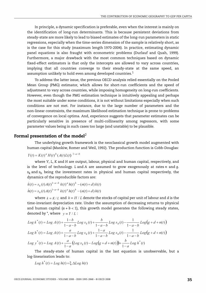
THE CONTRIBUTION OF ECONOMIC GEOGRAPHY TO GDP PER CAPITA
In principle, a dynamic specification is preferable, even when the interest is mainly on
the identification of long-run determinants. This is because persistent deviations from
steady-state are more likely to lead to biased estimates of the long-run parameters in static
regressions, especially when the time-series dimension of the sample is relatively short, as
is the case for this study (maximum length 1970-2004). In practice, estimating dynamic
panel equations is also fraught with econometric problems (Durlauf and Quah, 1999).
Furthermore, a major drawback with the most common techniques based on dynamic
fixed-effect estimators is that only the intercepts are allowed to vary across countries,
implying that all countries converge to their steady-state at the same speed, an
assumption unlikely to hold even among developed countries.1
To address the latter issue, the previous OECD analysis relied essentially on the Pooled
Mean Group (PMG) estimator, which allows for short-run coefficients and the speed of
adjustment to vary across countries, while imposing homogeneity on long-run coefficients.
However, even though the PMG estimation technique is intuitively appealing and perhaps
the most suitable under some conditions, it is not without limitations especially when such
conditions are not met. For instance, due to the large number of parameters and the
non-linear constraints, the maximum likelihood estimation technique is prone to problems
of convergence on local optima. And, experience suggests that parameter estimates can be
particularly sensitive in presence of multi-collinearity among regressors, with some
parameter values being in such cases too large (and unstable) to be plausible.
Formal presentation of the model2
The underlying growth framework is the neoclassical growth model augmented with
human capital (Mankiw, Romer and Weil, 1992). The production function is Cobb-Douglas:
where Y, L, K and H are output, labour, physical and human capital, respectively, and
is the level of technology. L and A are assumed to grow exogenously at rates n and g.
sk and sh being the investment rates in physical and human capital respectively, the
dynamics of the reproducible factors are:
where and denote the stocks of capital per unit of labour and d is the
time-invariant depreciation rate. Under the assumption of decreasing returns to physical
and human capital (a + b < 1), this growth model generates the following steady states,
denoted by *, where :
The steady-state of human capital in the last equation is unobservable, but a
log-linearisation leads to:
baba tLtAtHtKtY −−= 1))()(()()()(
)())(()()()()()(
)())(()()()()()(1
1
thdtnthtktAtsth
tkdtnthtktAtstkbaba
h
babak
+−=
+−=−−
−−
&
&
LKk /≡ LHh /≡
LYy /≡
( )
( )
( )( ) )(1
)()(1
)()(
)(1
1)(1
1)(1
)()(
)(1
1)(1
)(1
1)()(
**
*
*
thLoga
btndgLogtsLoga
atALogtyLog
tndgLogba
tsLogba
atsLogba
atALogthLog
tndgLogba
tsLogba
btsLogba
btALogtkLog
k
hk
hk
−+++−
−+=
++−−
−−−
−+
−−+=
++−−
−−−
+−−
−+=
)(.)()(* thLogthLogthLog Δ+= ξ
OECD JOURNAL: ECONOMIC STUDIES – VOLUME 2008 – ISSN 1995-2848 – © OECD 2008 35
THE CONTRIBUTION OF ECONOMIC GEOGRAPHY TO GDP PER CAPITA
being a function of the technological parameters (a,b). Consequently, the income
steady-state is given by the following level equation:
(level equation)
The level equation ignores the dynamics to the steady state. A linear approximation of
the transitional dynamics can be expressed as follows:
where is the annual speed of convergence and
is a constant. In order to obtain the error-correction form, short-run dynamics
around the transition path has to be accounted for. Taking the maximum lag as being one,
the following is obtained:
(error correction equation)
The error correction equation could be estimated by imposing the homogeneity of all
the coefficients across countries. Such restrictions are generally not supported by the data.
An alternative specification, the Pooled Mean Group, proposed by Pesaran, Shin and Smith
(1999) consists in allowing short-run coefficients, the speed of adjustment and error
variances to differ across countries, while imposing homogeneity on long-run coefficients.
Formally, the following specification is estimated:
(error correction equation, PMG)
It is common to impose (g + d) in Log[g + d + n(t)] to be equal to 0.05. Based on
the Cobb-Douglas production function, the physical and capital shares are equal to a
and b, respectively. These two parameters should therefore be around 1/3.
Consequently, the coefficients that are consistent with the model above should be
close to 0.5 for both Log sk and Log sh, with a speed of convergence of around
.
The empirical framework above is actually fairly general and consistent with various
endogenous growth models, but with different interpretation of the parameters (Bernanke
and Gürkaynak, 2001). In particular, the Uzawa-Lucas model generates the following steady
state (Piras, 1997; Bassanini and Scarpetta, 2001):
where is the steady-state growth rate of GDP per capita, which is the sum of
the exogenous growth rate, g, and of the equilibrium growth rate of human capital per
effective unit of labour, . Therefore, one can still assume . Thus, the
steady-state equation is similar to that obtained in the augmented Solow model, but with
( ) g tALogthLoga
bthLoga
btndgLoga
atsLoga
atyLog k ++Δ−
+−
+++−
−−
= )0()(1
)(1
)(1
)(1
)(* ξ
( ) ⎥⎦
⎤⎢⎣
⎡⎟⎠⎞
⎜⎝⎛ ++Δ
−+
−+++
−−
−−−−=Δ
⇔+−−=
ψξλ
λλ
tgthLoga
bthLoga
btndgLoga
atsLoga
atyLogtyLog
tyLogtyLogtyLog
k )(1
)(1
)(1
)(1
)1()(
)()1()1()( *
)()1( ndgba ++−−≡λ ψ )0( += ALogλλ /)1( −g
( )
( ) )()()()(
)(1
)(1
)(1
)(1
)1()(
243210 thLogathLogatndgLogatsLogaa
tgthLoga
bthLoga
btndgLoga
atsLoga
atyLogtyLog
k
k
Δ+Δ+++Δ+Δ++
⎥⎦
⎤⎢⎣
⎡⎟⎠⎞
⎜⎝⎛ +Δ
−+
−+++
−−
−−−−=Δ ξλ
( )
( )2
243210
)(,and across i.i.d.
)()()()(
)(1
)(1
)(1
)(1
)1()(
iitit
itiiiiiikiii
iiikiiii
Varti
thLogathLogatndgLogatsLogaa
tgthLoga
bthLoga
btndgLoga
atsLoga
atyLogtyLog
σεε
ε
ξλ
=
+Δ+Δ+++Δ+Δ++
⎢⎣
⎡⎟⎠⎞
⎜⎝⎛ +Δ
−+
−+++
−−
−−−−=Δ
023.0)0 2.00 5.0).(3/13/11()()1( ≈+−−≈++−− ndgba
( ) g tALogthLogtndgLoga
atsLoga
atyLog k +++++−
−−
= )0()()(~1
)(1
)(*
*~
hgg γ+≡
*hγ 0 5.0~ =+ dg
OECD JOURNAL: ECONOMIC STUDIES – VOLUME 2008 – ISSN 1995-2848 – © OECD 200836
THE CONTRIBUTION OF ECONOMIC GEOGRAPHY TO GDP PER CAPITA
the prediction that the coefficient for human capital is equal to one. The transitional
dynamics along the stable path is:
with the speed of convergence given by: . There are two
differences with the transitional dynamics in the augmented Solow model. First, the
human capital coefficient is equal to one in the Uzawa-Lucas model instead of around 0.5
in the augmented Solow specification. Second, the speed of convergence is much faster in
the Uzawa-Lucas approach, as a reasonable order of magnitude is
instead of 0.02 previously.
Notes
1. The implications of imposing invalid homogeneity restrictions on slope parameters in the contextof dynamic panel estimates are discussed in Lee, Pesaran and Smith (1997).
2. This section borrows from Bassanini and Scarpetta (2001).
( ) ⎥⎦
⎤⎢⎣
⎡⎟⎠⎞
⎜⎝⎛ ++Δ++++
−−
−−−−=Δ ψξλ tgthLogthLogtndgLog
aatsLog
aatyLogtyLog k )()()(~
1)(
1)1(~)(
aandg /)1()~(~−++≡λ
).3/1/()3/11(~
−≈λ1 4.0)0 2.00 5.0( ≈+
OECD JOURNAL: ECONOMIC STUDIES – VOLUME 2008 – ISSN 1995-2848 – © OECD 2008 37

Related Documents