THE CONTINUOUS WAVELET TRANSFORM: A … SADOWSKY THE CONTINUOUS WAVELET TRANSFORM: A TOOL FOR SIGNAL INVESTIGATION AND UNDERSTANDING In this article, the continuous wavelet transform

JOHN SADOWSKY

THE CONTINUOUS WAVELET TRANSFORM: A TOOL FOR SIGNAL INVESTIGATION AND UNDERSTANDING

In this article, the continuous wavelet transform is introduced as a signal processing tool for investigating time-varying frequency spectrum characteristics of nonstationary signals. The transform is discussed within the context of Fourier methods and the general problem of time-frequency representation and is compared with the more traditional Gabor method of windowed Fourier transforms. To take full advantage of the potential benefit of wavelet characterization, a computer algorithm for generating wavelet images from data is needed. Such an efficient algorithm, the algorithme a trous, was invented and published several years ago by an important group of engineering researchers. A detailed derivation and analysis of their algorithm is presented.

INTRODUCTION Five to 10 years ago, the theory of wavelets caught the

imagination of researchers in harmonic analysis, signal and image processing, and applied science as the new methodology, promising to usurp the throne occupied by Fourier analy is and solve the problems that have con­founded cla sical analysts for hundreds of years. Five years ago I met with Dr. Howard Resnikoff, president of Aware, Inc. , and an early advocate of the potential of wavelets. He declared that some of the most important problems in applied mathematics were being solved by a group of French mathematicians and scientists using new tool for analyzing signals in new types of basis functions. He advi ed us to learn about wavelets if we wished to remain on the cutting edge of signal and image processing. Dr. Resnikoff is a well-respected scholar in applied mathematics and signal processing, so his level of enthusia m conveyed a sense that yet another major breakthrough in science was occurring.

Wavelet analysis is indeed an important development in mathematics, science, and engineering. Rather than replacing Fourier methods, however, it complements and extends the e cla sical approache , solving problems for which Fourier analysis is unsuited and failing in cases for which Fourier analysis is ideal. One cannot design wave­let bases and analyze the wavelet transform without sig­nificant use of Fourier methods.

Moreover, the roots of wavelet analysis reach back almost 100 years. They can be found in a variety of sciences, from quantum mechanics and Brownian motion to the mathematical works of Littlewood and Paley in the 1930s, Gabor in the 1940s, and Calderon in the late 1950s. Meyer I presents an excellent, though terse, over­view of the history of wavelet analysis.

Wavelet analysis is an essential addition to the toolbox of researcher and developers in the field of signal processing. Important and exciting new systems planned at the Laboratory could benefit greatly from wavelet­based proce ors. Applications of wavelet technology at

306

APL include essential defense needs (e.g., signal intelli­gence, smart weapons, command and control, and com­munications systems), space and oceanographic data analysis , biomedical systems (e.g., medical imaging systems, speech and visual processing systems, and biological sensor monitoring), and basic science research and development.

This article is the first in a erie planned for the fohns Hopkins APL Technical Digest to introduce and explore this growing and fascinating field. This first article begins with the definition of wavelets, the wavelet transform, and bases of wavelets and then derives an algorithm for the continuous wavelet transform (CWT). The second article will examine data processed with the algorithm to inves­tigate how the signal parameters and characteristics are manifest in the complex surface of a wavelet transform. Future articles will explore the atomic decomposition of signals and images with respect to wavelet bases and frames and the application of wavelet technologies to signal analysis , signal and image compression, and pat­tern recognition; computational algorithms for such ap­plications; and the use of wavelet-based processing in APL systems and problems.

WHAT IS A WAVELET? There are several approaches to understanding the

nature of wavelet analysis. These different approaches­actually, different perspectives of the arne overall con­cept-reflect different taste, styles, and areas of appli­cation among researchers (see Refs. 1-4 for varied point of view). One pos ible approach is from the viewpont of time-frequency representations of nonstationary and wideband signals. Consider a mu ical composition, for example. Our emotional and intellectual response to music results from the time variation of the frequency spectrum of the music-different notes are played at dif­ferent times. A Fourier transformation of a piece of music does not directly represent this time variation of spectrum.

Johns Hopkins APL Technical Digest, Volume 15, Number 4 (1994)

A A n 4 1 :3 S", 5i " A

I ., --.....J - - .W!"*!~ ~ iJ

~ A

I ~ .~ . .-..

• • ~ ~

I n

eJ

r.~ J j j J A

" AI J J I

I. I. I. I. I l I [ r y y

The frequencies present in the music are certainly visible in a Fourier transformation, but the time-dependence seems to be lost.

Of course, the time-dependence cannot actually be lost because an inverse Fourier transform of the spectrum will re-create the piece of music. (I am making the mathema­tician 's assumption that the music is of infinite duration and that the spectrum is complete, from -00 to 00 in both cases.) The time variation is contained in the phase of the Fourier spectrum, however, in a way that is inconsistent with the way that musicians create music. The Fourier spectrum contains frequencies that are not present in the piece of music but rather at phases such that coherent superposition of frequencies causes the proper amount of destructive interference to cancel notes not present at specific times. It is as if musicians were specifically playing notes not in the score, phased so as to cancel out some notes to produce proper durations of other notes.

Music, however, occurs because musicians play notes to be heard at specific times and for specific durations. These notes and times of performance are well repesented in the musical score (Fig. 1). Here, the horizontal axis represents time and the vertical staff indicates frequency (notes) to be played at specific times. Durations are in­dicated by the types of notes (quarter, half, whole, etc.), times of absence of frequencies for specific instruments are indicated by rests, and amplitudes of frequncies are indicated by notations for crescendos, diminuendos, and other dynamic markings (such as piano and forte). The score is a good representation of the music in time (hor­izontal) and frequency (vertical). A problem in time­frequency representation is to design a signal processing system that will produce the score from the music.

Wavelet theory offers a novel approach to this problem and, as such, can be seen as an extension and enhance­ment of the Gabor windowed Fourier transform method for time-frequency representation (see, for example, Meyer' and Daubechies2

) . In the Gabor method, we define a finite-duration window wet) as shown in Fig. 2. By translating this window in time and multiplying it by the signal set), we obtain a chunk of the signal over a particular small piece of time. If the window is nonzero between - T12 and T12 , for example, then the product s(t)w(t - to) is an approximation to the signal in the time interval from to - T12 to to + T12. That is, the product selects a portion of the signal of duration T centered at

Johns Hopkins APL Technical Digest, Volume 15. Number 4 (/994)

• I

mf

:'

A ~

I I

Time series

Figure 1. Example of an effective time­frequency representation , a musical score.

Window of duration T centered at to

to - TI2 to to + TI2

Portion of time series restricted by the window

1

Figure 2. Restriction of the time duration of a time series with a Gabor window (Gaussian) .

time to. The Gabor windowed Fourier transform is then defined to be the Fourier transform of this windowed signal:

1 foo -iwf G(w, to) = ~ s(t)w * (t - to)e dt, ,, 27r -00

where * denotes the complex conjugate. Although the window often is real, we have written the Gabor transform in its more general form. Also, we will denote signals, that is, functions of the time variable t, with lowercase Latin and Greek letters and the Fourier transforms of signals with

307

1. Sadowsky

uppercase Latin and Greek letters. Thus, for example, the Fourier transform of the signal fit) is

1 foo h -iwtd F(w) = r;:;- J (t)e t \j 271" -00

The frequency variable in the Fourier transform is in units of radians per second, for consistency with the wavelets literature, and i denotes -1.

This transform is a time-frequency representation as well as a function of time to and frequency w, and provides an approximation to the frequency content of the signal over a small time interval about time to. If the window is well concentrated in time and frequency, as is the case, for instance, with a Gaussian window, then this time­frequency representation is reasonable for some applica­tions. It has limitations, however. For example, resolution in frequency is a function of the duration of the window; the longer the window duration, the finer the frequency resolution. Conversely, increasing the window duration will smear a rapidly changing time variation in the spectrum.

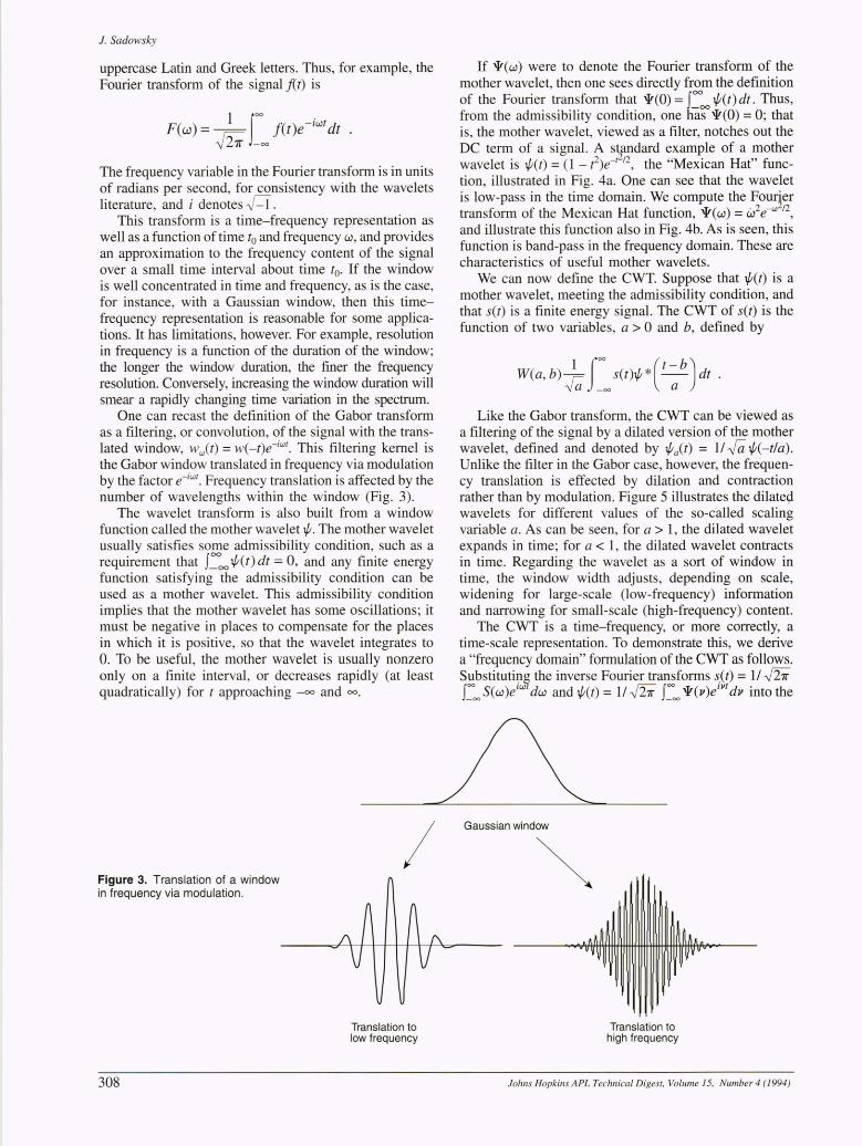
One can recast the definition of the Gabor transform as a filtering, or convolution, of the signal with the trans­lated window, ww(t ) = w (_t)e-

iwt. This filtering kernel is

the Gabor window translated in frequency via modulation by the factor e -

iwt. Frequency translation is affected by the

number of wavelengths within the window (Fig. 3). The wavelet transform is also built from a window

function called the mother wavelet t/;. The mother wavelet usually satisfies some admissibility condition, such as a requirement that f~oo t/;(t) dt = 0, and any finite energy function satisfying the admissibility condition can be used as a mother wavelet. This admissibility condition implies that the mother wavelet has some oscillations; it must be negative in places to compensate for the places in which it is positive, so that the wavelet integrates to O. To be useful, the mother wavelet is usually nonzero only on a finite interval, or decreases rapidly (at least quadratically) for t approaching -00 and 00.

Figure 3. Translation of a window in frequency via modulation.

308

/

Translation to low frequency

If '!r(w) were to denote the Fourier transform of the mother wavelet, then one sees directly from the definition of the Fourier transform that '!reO) = f:'oo t/;(t) dt. Thus, from the admissibility condition, one has '!reO) = 0; that is, the mother wavelet, viewed as a filter, notches out the DC term of a signal. A standard example of a mother wavelet is t/;(t) = (1 - (2 )e-t212

, the "Mexican Hat" func­tion, illustrated in Fig. 4a. One can see that the wavelet is low-pass in the time domain. We compute the Fourier transform of the Mexican Hat function, '!r(w) = "le-w

212,

and illustrate this function also in Fig. 4b. As is seen, this function is band-pass in the frequency domain. These are characteristics of useful mother wavelets.

We can now define the CWT. Suppose that t/;(t) is a mother wavelet, meeting the admissibility condition, and that set) is a finite energy signal. The CWT of set) is the function of two variables, a> 0 and b, defmed by

1 f oo (t-b) W(a, b) -Fa. - 00 s(t)t/;* -a- dt .

Like the Gabor transform, the CWT can be viewed as a filtering of the signal by a dilated version of the mother wavelet, defined and denoted by t/;a(t) = 1/ -J(i t/;(-tla). Unlike the filter in the Gabor case, however, the frequen­cy translation is effected by dilation and contraction rather than by modulation. Figure 5 illustrates the dilate<iI wavelets for different values of the so-called scaling variable a. As can be seen, for a > 1, the dilated wavelet expands in time; for a < 1, the dilated wavelet contracts in time. Regarding the wavelet as a sort of window in time, the window width adjusts, depending on scale, widening for large-scale (low-frequency) information and narrowing for small-scale (high-frequency) content.

The CWT is a time-frequency, or more correctly, a time-scale representation. To demonstrate this, we derive a "frequency domain" formulation of the CWT as follows. Substitutipg the inverse Fourier transforms s.ct) = 1/.J2i f~oo S(w)elwtdw and t/;(t) = 1/.J2i f~oo '!r(v)e1/ltdv into the

Gaussian window

Translation to high frequency

f ohns Hopkins APL Technical Digest, Volume 15, Number 4 (1994)

(a) t{t(t)

(b) 'lr(w)

w

Figure 4. The Mexican Hat wavelet an~ its Fourier transform. (a) Mexican Hat function , t{t(t) = (1 - t 2)e-t /2. (b) Fourier transform of the Mexican Hat function , ir(w) = w2e-w

2/2.

formula for W(a, b), integrating the resulting Dirac 0-function, and simplifying, one obtains

W(a, b) = -Jaf~oo S(w)'lr * (aw)eiwb

dw.

We see that the CWT can be viewed as a frequency­domain filtering of the signal by the dilated filter .JCi 'J! (aw) . Figure 6 illustrates this dilation filter (in the frequency domain) for the Mexican Hat wavelet. As can be seen, the large-scale case, a » 1, has the filter com­pressed to small-bandwidth (fine-resolution), low­frequency parts of the spectrum; the small-scale case, a « 1, has the filter expanded to wide-bandwidth (coarser­resolution), high-frequency parts of the spectrum. Scale has the relationship to frequency that one would expect, and the frequency resolution of the CWT adjusts such that the ratio of frequency resolution to frequency is constant. Not only is this frequency-dependent resolution consistent with the performance of visual and auditory systems, but it also permits an efficient computation of a range of frequencies, without the need to set a fixed, high resolution and compute redundant information when lower resolution would suffice.

The preceding paragraph describes the zoom-in prop­erty of the CWT. A wavelet transform zooms in on the fine detail and zooms out on the coarser trends of a signal.

Johns Hopkins APL Technical Digest, Volume 15, Number 4 (1994)

The Continuous Wavelet Transform

W(a, b)

Decrease scale, a=0.3 / W(a, b) /' \

l nCr~a!~~~ale ,

W(a,b)

Figure 5. Frequency translation of the Mexican Hat function via scaling (dilation): time domain.

Decrease scale,J a= 0.3 W(a, b)

W(a, b)

\ Increase scale, a= 3.0 W(a, b)

Figure 6. Frequency translation of the Mexican Hat function via scaling (dilation): frequency domain .

This property distinguishes the CWT from the Gabor transform, for which the frequency resolution is preset and is independent of the detail or coarseness of the parts of the signal being analyzed. In addition, this frequency­dependent resolution is the basis for the application of wavelet analysis to multiresolution decomposition, that

309

1. Sadowsky

is, decomposition of signals and images that represent a range of different resolution scales. Multiresolution de­composition with wavelets will be a topic in a future article about the discrete wavelet transform.

The CWT produce a complex-valued surface, as it is a function of two variables, a and b. Following conven­tion, the b axis (time) is drawn horizontally and the a axis (scale, or frequency) is drawn vertically. Because the variable a is po itive, the a axis is actually a ray. We draw the a axis oriented downward, so that smaller values of a, corresponding to higher frequencies , are above larger values of a, corresponding to lower frequencies (Fig. 7). Some researchers prefer to represent the scale axis log­arithmically, in which case the log(a) axis extends be­tween -00 and 00. In thi case, the orientation of the axis remain downward for increasing values of a.

To understand the CWT surface, consider local influ­ences on the surface from the signal and local parts of

(a) (0,0)

the signal that affect the surface.s In particular, we wish to identify the region of the CWT surface that is influ­enced by the value of the signal at a particular time to and the particular time intervals of the signal that contribute to a specific point (ao, bo) in the CWT surface.

Assume that the mother wavelet has support which is an interval A; that is, 1/!(t) is zero for t not in A. From the time-domain definition of the CWT, one can see that, if we fix the variable a and b, then the integral is com­puted over the interval aA + b. Thus, for time to to be of influence one must have to - aq :s; b :s; to - ap, where the interval A has endpoints p and q. Where the interval is centered about the origin, for example, this describes a cone in the ab plane with vertex at the point to on the b axis, as is shown in Fig. 7b.

Similarly, the point (ao, bo) in the CWT surface is influenced by signal values at times in the interval aoA + boo This can be illustrated with an upward cone

+b

Negative

+b

Positive Increasing a

Linear scale variable Logarithmic scale variable

Figure 7. Representation ofthe CWT sur­face. (a) The coordinate axes for image representations of the CWT. (b) Cone of influence of a time point of the signal on the surface. (c) Cone of influence of a point on the surface on an interval in time.

310

(b)

(c)

s(t) to +-------'---'-..----.-- -.b

a

Width = ao x support ~ length of the wavelet

s(t) bo +------'----'-r---,------,-,~ b

a

Width = ao x support length of the wavelet

Johns Hopkins APL Technical Digest, Volume 15, Number 4 (1994)

with vertex to (Fig. 7b) , where the interval on the b axis in the cone represents the time interval of the signal that affects the point in the CWT surface.

Grossmann et al. 5 suggest a method for representing the complex values of the surface without having to draw separate real and imaginary surfaces or amplitude and phase surfaces. In their method, complex amplitude is represented by color from a lookup table, and phase is represented by a density of black dots overdrawn on the colors, from no black dots (phase 0) to total saturation (phase 27r).

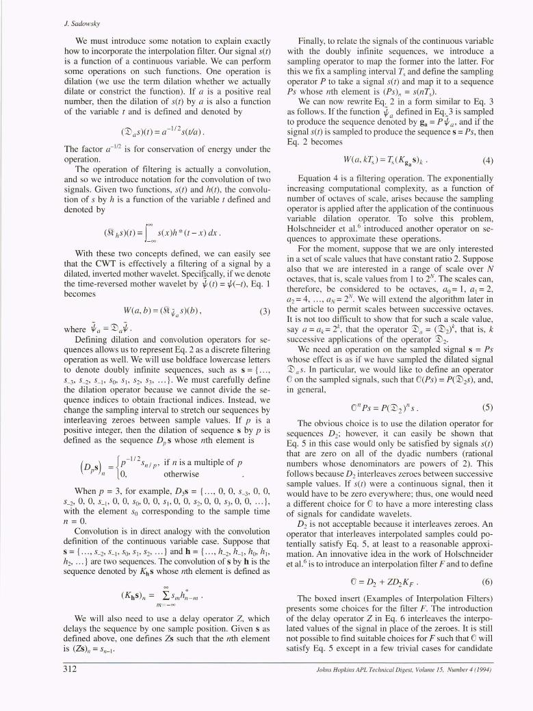
As a small modification to this approach, we reverse the roles of the dot density and color. Each pixel can be expanded to a 4 X 4 alTay of subpixels or dots. Normal­ized amplitude is represented as the number of subpixels that are colored in the surface, from zero (for an ampli­tude of 0 or sufficiently small) to all 16 (for an amplitude of 1 or sufficiently high). The particular subpixels to color are selected randomly. Thus, amplitude is reflected in the surface by sparseness to saturation of color. The phase is color-coded using a lookup table. Figure 8 is an example of a CWT surface generated from actual data from an interrnittant process, which illustrates this concept.

The rest of this article reviews the mathematical basis for the CWT algorithm used to generate the surface in Fig. 8.

ALGORITHM FOR THE CONTINUOUS WAVELET TRANSFORM

In this section we derive an algorithm for computing the CWT. The approach follows closely the derivation and data flow diagrams of Holschneider et al. 6 with added

(a)

Q) "0 . .e

-5

g- -10 -<

-15

50 100 150

(b) Time

Johns Hopkins APL Technical Digest, Volume 15, Number 4 (1994)

The Continuous Wavelet Transform

detail and carefully computed filter delays and algorithm constructions. The algorithm explicitly recognizes that the CWT can be realized with several filters, all of which are dilations of a single filter. Their construction intro­duces the method of the algorithme it trous for efficiently implementing such a structure.

To motivate the need for such an algorithm, we consider a numerical approximation to the integral in the CWT:

If the signal set) is sampled with sampling interval Ts'

then the CWT at the time step b = kTs is approximated by the sum

The summation is essentially over the range of sam­ples of the signal set). The computational problem arises from the scaling factor a in the denominator of the ar­gument of the sampled wavelet. Because of this denom­inator, the wavelet must be resampled at a sampling interval of Tia for the wavelet transform at scale a. If, for example, we wish to display the CWT over 10 oc­taves, the high-scale computational complexity (size of the summation) increases by a factor of 210 = 1024. The algorithm by Holschneider et al.6 solves this problem for certain classes of wavelets by replacing the need to resample the wavelet with a recursive application of an interpolating filter.

200 250

Figure 8. Example of a CWT surface generated from actual data from an inter­mittent process. (a) Section of the time series. (b) CWT of the time series. The horizontal axis is increasing time and the vertical axis is scale (frequency-related) from small (top of figure) to large (bottom of figure). Concentration of color reflects amplitude and color reflects phase. Inter­esting structure is found in the phase; however, three peaks appear in the image-two at the left and one in mid­image toward the right.

311

1. Sadowsky

We must introduce some notation to explain exactly how to incorporate the interpolation filter. Our signal set) is a function of a continuous variable. We can perform some operations on such functions. One operation is dilation (we use the term dilation whether we actually dilate or constrict the function). If a is a positive real number, then the dilation of set) by a is also a function of the variable t and is defined and denoted by

(SDas)(t) = a- i !2s(tla).

The factor a-1/2 is for conservation of energy under the operation.

The operation of filtering is actually a convolution, and so we introduce notation for the convolution of two signals. Given two functions, set) and h(t), the convolu­tion of s by h is a function of the variable t defined and denoted by

(S'r hs)(t) = f~oo s(x)h * (t - x) dx .

With these two concepts defined, we can easily see that the CWT is effectively a filtering of a signal by a dilated, inverted mother wavelet. Speciflcally, if we denote the time-reversed mother wavelet by 1/; (t) = 1/;(-t), Eq. 1 becomes

W(a, b) = (Sf ~as)(b), (3)

where ~a = §)a~' Defining dilation and convolution operators for se­

quences allows us to represent Eq. 2 as a discrete filtering operation as well. We will use boldface lowercase letters to denote doubly infinite sequences, such as s = { ... , L3, L2, Ll> So' Sl> S2, S3, ".}. We must carefully define the dilation operator because we cannot divide the se­quence indices to obtain fractional indices. Instead, we change the sampling interval to stretch our sequences by interleaving zeroes between sample values. If p is a positive integer, then the dilation of sequence s by p is defined as the sequence Dp s whose nth element is

(D s) = {p-1I2 Sn / p' if n is a multiple of p

p n 0, otherwise .

When p = 3, for example, D3S = { ... , 0, 0, L3, 0, 0, S_2' 0, 0, Lj, 0, 0, so, 0, 0, Sl> 0, 0, S2'0, 0, S3, 0, 0, ... }, with the element So corresponding to the sample time n = 0.

Convolution is in direct analogy with the convolution definition of the continuous variable case. Suppose that s = {"., S_2' Ll> So' Sl> S2, ".} and h = {. '" h_2' h_I' ho, hi' h2' ... } are two sequences. The convolution of s by h is the sequence denoted by Kh s whose nth element is defined as

00

(Khs)n = LSmh,:_m· m=-oo

We will also need to use a delay operator Z, which delays the sequence by one sample position. Given s as defined above, one defines Zs such that the nth element is (Zs)n = Sn_I'

312

Finally, to relate the signals of the continuous variable with the doubly infinite sequences, we introduce a sampling operator to map the former into the latter. For this we fix a sampling interval Ts and define the sampling operator P to take a signal s(t) and map it to a sequence Ps whose nth element is (Ps)n = s(nTs) '

We can now rewrite Eq. 2 in a form similar to Eq. 3 as follows. If the function ~ a defined in Eq:,.3 is sampled to produce the sequence denoted by ga = P 1/; a' and if the signal set) is sampled to produce the sequence s = Ps, then Eq. 2 becomes

(4)

Equation 4 is a filtering operation. The exponentially increasing computational complexity, as a function of number of octaves of scale, arises because the sampling operator is applied after the application of the continuous variable dilation operator. To solve this problem, Holschneider et a1.6 introduced another operator on se­quences to approximate these operations.

For the moment, suppose that we are only interested in a set of scale values that have constant ratio 2. Suppose also that we are interested in a range of scale over N octaves, that is, scale values from 1 to 2N. The scales can, therefore, be considered to be octaves, ao = 1, al = 2, a2 = 4, ... , aN= 2N. We will extend the algorithm later in the article to permit scales between successive octaves. It is not too difficult to show that for such a scale value, say a = ak = 2k, that the operator §)a = (§)2)k, that is, k successive applications of the operator §)2'

We need an operation on the sampled signal s = Ps whose effect is as if we have sampled the dilated signal §) as' In particular, we would like to define an operator o on the sampled signals, such that O(Ps) = P(§)2S), and, in general,

(5)

The obvious choice is to use the dilation operator for sequences D2 ; however, it can easily be shown that Eq. 5 in this case would only be satisfied by signals s(t) that are zero on all of the dyadic numbers (rational numbers whose denominators are powers of 2). This follows because D2 interleaves zeroes between successive sample values. If set) were a continuous signal, then it would have to be zero everywhere; thus, one would need a different choice for to have a more interesting class of signals for candidate wavelets .

D2 is not acceptable because it interleaves zeroes. An operator that interleaves interpolated samples could po­tentially satisfy Eq. 5, at least to a reasonable approxi­mation. An innovative idea in the work of Holschneider et a1.6 is to introduce an interpolation filter F and to define

(6)

The boxed insert (Examples of Interpolation Filters) presents some choices for the filter F. The introduction of the delay operator Z in Eq. 6 interleaves the interpo­lated values of the signal in place of the zeroes. It is still not possible to find suitable choices for F such that 0 will satisfy Eq. 5 except in a few trivial cases for candidate

Johns Hopkins APL Technical Digest, Volume 15, Number 4 (1994)

wavelet signals. Thus, another idea introduced by Holschneider et al. is to relax the requirement of Eq. 5 to the approximation case. First, one fixes a tolerance c > 0 and a maximum number of octaves N. Then Eq. 5 becomes

Ilonps - P(~2tsll < c, for 0 ::; n::; N . (7)

The notation II II denotes the norm in the space of sequences and is defined such that:i for g = { ... , g-2' g-b go, g], g2, ... }, IIgll = (L.-;=-ool gn I )1/2 . For a particular choice of wavelet signal set) and interpolating filter F, and for explicit range N and tolerance c, the condition in Eq. 7 can be numerically verified. This verification is performed as part of the selection of algorithm parameters. An oper­ator 0 satisfying Eq. 7 is called a pseudo-dilation operator.

Holschneider et a1.6 showed that, for a selection of interpolating filter and a pseudo-dilation operator 0, as defined in Eq. 6, the filtering operation for the CWT presented in Eq. 4 can be factored into simple filtering operations. Moreover, these simple filters are recursively related to each other, thus facilitating an algorithme a

EXAMPLES OF INTERPOLA TION FILTERS Here we consider the effect of (!J = D2 + ZD2KF for var­

ious interpolation filters F. Only the nonzero elements of the impulse response for F will be shown.

First, suppose that the impulse response to F is {fo = I} (and all other samples are therefore zero). Then the convo­lution of a signal s with F produces (KFs)1l = Sn- Thus,

if n is even

if n is odd .

Thus, this simple filter merely stretches the signal and interleaves a repeat of each sample so that { .. . , L3, L2, L), So'

sl, s2, S3,"'} becomes { ... , L3, L3, L2, L2, L), LJ, so, so, S), SJ, S20 S20 S3, S3, . . . }, appropriately scaled by 2- 112

.

As a second example, consider the interpolation filter F whose impulse response is {f-I =fo= 1/2} . One can com­pute at once that the operation of (!J on the signal s is

if n is even

if n is odd .

Ignoring the scale change by 2-1/2 for the moment, the sample at time 0 is So and the sample at time 2 is S I . The sample at time 1 is (so + sl)/2. Continuing for all times, one sees that this filter is a straightforward linear interpolator.

Similarly, we can construct polynomial interpolators by considering the effects of samples beyond the two adjacent samples. A cubic interpolator, for example, uses the filter F with impulse response {f-2 = -1/16, f - I = 9/16, fo = 9/16, fl = -1I16} . The interpolated value, in this case, between the samples Snl2 and Sn/2+1 is obtained by fitting a cubic poly­nomial to the samples Sn/2-J, snl2, Sn/2+" and Sn/2+2, and evaluating it at n12 + 112.

Johns Hopkins APL Technical Digest, Volume 15, Number 4 (1994)

The Continuous Wavelet Transform

trous approach to their implementation. The specific fac­toring is presented in the lemma below, whose proof is presented in the boxed insert (Proof of Lemma). Recall that the CW~ filtering is by the sequence ga = g2D. More­over, ga = p t/; a' and ~ ais defined in Eq. 3. Thus, _the CWT reguires a filtering by the sequence g2D = P~2n t/; = P(~2Y t/; =:= on(p t/;). For simplicity, let f denote the se­quence Pt/;. Then the CWT requires filtering by the sequence Onf, that is, the performance of the convolution, K /If.

LEMMA: Suppose that f is a sequence and that F is an interpolation filter defining the pseudo-dilation operator 0 = D 2 + ZD2K F. Then the convolution operator K Ollf can be factored as

(8)

where a = 1I .fi, and

fn = (a- ID2Yf , (9)

PROOF OF LEMMA We present here a proof of the lemma in the article. We

wish to prove that

KOllf = a nKfllKFIKF2 . .. KFn .

Recall that z-transforms change such operations into multiplications, and there is a one-to-one correspondence between sequences and their z-transforms. If we denote a z-transform of a sequence s by s(z), then it therefore suffices to prove that

«(!JIlO(Z) = allf ll(z)F I(z)F2(z) .. . FIl (z).

We prove this by induction on n. It is helpful to review the effects of the various operators

on the z-tranforms. The delay operator Z, for example, has the effect of multiplying the z-transform of the sequence by Z-I. The convolution operator KG has the effect of multiply­ing the z-transform of the sequence by G(z) . The dilation operator D2 has the effect of a change of variable to the z­transform as(z2) . Thus, if the operator (!J is applied to the sequence s, then the resulting sequence has z-transform, as(z2) + a z-I F(Z2)s(Z2) .

For n = 1, the computation is straightforward. From the preceding paragraph, one has

«(!JO(z) = af(z2) + az-I F(Z2)f (Z2) .

The z-transform of f l is computed, from its definition, to be f(i), and that of Fl is computed to be 1 + z-IF(z2), using the fact that the z-transform of D is 1. Thus, the convolution by aflFl is a multiplication by

a[f(z2)][1 + Z-IF(z2) ]

in the z-transform domain. But this is exactly «(!JO(z) . Now assume, via induction, that n ~ 2 and that

((!In-1o(z) = a n- 1f(z2n-I)[1 + z-lF(i) ] [1 + z-2F(z4)] ...

[1 + z- 21l-2F(z2n- l)] .

Applying (!J one more time evaluates the above at Z2 rather than z and multiplies it by a[1 + Z-l F(Z2)]. Carrying out these operations shows that the identity holds for n as well, completing the proof.

313

1. Sadowsky

(10)

and

(11)

In the lemma, 0 is the impulse sequence { ... , d_ l> do, d l , ••• } for which do = 1 and d; = 0 for i =1= O. Note also that the convolution operators in the factoring of Eq. 8 commute, and so the order of the filtering implied is not important.

The lemma presents a simple method for deriving the filtering convolution for the kth octave in terms of the filtering convolution for the (k - 1) octave, because from Eq. 9 one has f k = (a - ID2)fk_1> and this fact and Eq. 11 show that the convolutions for octave k can be computed from the convolutions from octave k - 1. The boxed insert (Computation of N + 1 Octaves) shows precisely how these octaves are computed; a data flow diagram of the computation is presented in Fig. 9. Here, arcs showing the flowdown of the (a- ID2) factor in the definitions of the filters Fi and fi are indicated. The algorithme a trous is a method for incorporating this flowdown as a se­quence of multiplexing operations.

We must first consider the relationship between con­volution with an arbitrary filter H and convolution with the dilated filter (a- ID2)H. Suppose the impulse response for H has nonzero taps hkO' hkO+

I' ••• , hkl , with ko :::; 0 :::;

k l • Although the filter H is not necessarily causal, its support is consistent with the idea of an interpolating filter. For example, the nth output, given sequence s as input, is

Outputn = hZo sn-ko + h;o+1 Sn-kO -1 + ... + hZ1 Sn-k1 •

The output at time n is a function of future inputs Sn+l through Sn+1kol' current input Sn' and past inputs Sn_1 through sn-kl' It interpolates past and future samples. If the convolution is performed with (a- 1D2)H, a direct calculation verifies that the output at time n is

kl Outputn = L.. hZSn- 2k .

k=ko (12)

The subscript on the S indicates an introduction of two delays on the input between successive filter taps. Thus, Fig. lOa illustrates a tapped delay line implementation of Eq. 12. Here, the output at time n requires "future" inputs to time n + 21kol. Similarly, Fig. lOb illustrates the iter­ative application of the dilation factor to produce the output when filtering with (a-1D2YH.

An alternative formulation of the architecture shown in Fig. 10 can be constructed using the multiplexer pro­cess and an interleaver process illustrated in Fig. 11. The multiplexer receives as input a sampled sequence and passes this input on an alternating basis onto two output sequences. The interleaver accepts two input sequences and interleaves them so as to construct a single output sequence. The implicit timing must be such that a mul­tiplexer followed by an interleaver acts as an identity processor. If, for example, the multiplexer is alternately placing outputs on output lines A, B, A, B, ... , the cycles

314

COMPUTATION OF N+ 1 OCT A YES OF THE CWT Suppose S is the sampled input signal and f = P t/; for the

wavelet t/;. The octaves of the CWT are computed as follows:

Octave 0:

Octave 1:

For k = 2, ... , n

Output Kfs

Define Fl = 0 + T(a- ID2)F Define fl = (a-1D2)f Compute XI = aKFIs Output KflX1

Octave k: Define Fk = (a-1D2)Fk_1 Define f k = (a -I D2)fk- 1 Compute Xk = aKFkXk- 1 Output KfkXk

.j.: Octave a

CX-102

~Octave1 t (X-1 O2

'2 Octave 2

Octave 3

Octave N

Figure 9. Data flow diagram of the CWT over N + 1 octaves. The blue arrows indicate modifications to construct a filter from a previous filter via the dilation operator. Rectangles represent filtering operations (convolutions) and circles represent amplifica­tion (multiplication).

with output on line A must be synchronous with inter­leaver inputs from line A, and similarly for line B. This assumes a pairing of multiplexers and interleavers.

Figure 12 can easily be derived as an alternative implementation of the filters (a-1D 2)H and (a-1D2)JH using multiplexers and interleavers. The multiple input interleaver in Fig. 12b is synchronized so that the con­structed signal is correctly timed. This synchronization is somewhat tricky. For a three-stage (j = 3) implementa­tion, for example, the interleaving is constructed, in order, from legs 1, 5, 3, 7, 2, 6, 4, and 8. In the re-sorting of

Johns Hopkins APL TechnicaL Digest, VoLume 15, Number 4 (1994)

(a)

(b)

Sequence s >-Interleaver

Multiplexer

Sequence s Sequence s

Identity processor

Figure 11. Definition of multiplexer and interleaver processors.

the graph representation of the algorithm, described below, this ordering is automatically performed.

Now, to construct the CWT algorithm, we must replace the arbitrary filter H with specific filters. Equa­tions 9 and 11 in the lemma show that the filters f and FI = 0 + T(a- 1D 2)F are iteratively dilated and so H in the

Johns Hopkins APL Technical Digest, Volume 15, Number 4 (1994)

(a)

(b)

Output at time n

Output at time n

The Continuous Wavelet Transform

Figure 10. Tapped delay line imple­mentation of the dilated H filter. The sample delay operator T is denoted by its z-transform Z-1. Weights are com­plex conjugates ofthe impulse response for H. (a) Effect of a single dilation operation on the filter H. (b) Effect of j iterations of the dilation operation on the filter H.

--I ~~ t: t:

• • •

t: t:

Figure 12. Implementation of a dilation of a filter using multiplexers and ~n inter!eaver. ~a) Multiplexer/~nterlea~er implem~ntation of the dilated filter (a- D2)H. (b) Multlplexer/lnterleaver Implemen­tation of the dilated filter (a-1D2}'H.

315

1. Sadowsky

preceding discussion will be replaced by these two filters. The effect will be an expansion of the vertical and diag­onal flows of Fig. 9 using the multiplexer/interleaver diagrams of Figs. 10--12. This more complicated flow diagram can be sorted out into an elegant algorithm, as will be seen presently.

Consider next the specific computation of convolution with F J = 0 + Ta- JD2F. Assume that F has an impulse response whose nonzero terms are Wko' Wko , ... , Wk ,

with ko ~ ° ~ k J • It is a simple calculation to ~6e that th~ impulse response to F J is

{

I, if n = ° (Pi)n = w (n-l)I2, if n is odd and 2ko + 1 ~ n ~ 2ko + 1

0, otherwise. (13)

Substituting Eq. 13 into the formula for the convolu­tion, we compute that the output at time n of the filtering of sequence s by F

J is

(a)

k J

sn + L.. wksn-2k-l . k=ko

lkol - 1 delays

denote

and - IL ___ F __ ---.J~ denote

(14)

The form of the summation in Eq. 14 is similar to the convolution in Eq. 12, except for the delay by one (time is n - 1 rather than n). It can therefore also be implement­ed with multiplexers and interleavers as before. More­over, the additional term Sn is such that if n is odd, then the subscripts of the S term in the sum, n - 2k - 1, are all even and if n is even, then the subscripts are all odd. Thus, if we implement this form for F

J using multiplexers and

interleavers, then for each of the two legs out of the multiplexer in Fig. 12, there must be a tap in the opposite leg with which to sum. In other words, the top output of the multiplexer is summed with a specifically tapped register from the bottom leg, and the bottom output of the multiplexer is summed with a specifically tapped register from the top leg. Figure 13a presents a careful determi­nation of where these two taps should be, and Fig. 13b presents an implementation flow graph of this convolu­tion, using these tapped convolution processors.

Finally, we place the resulting processors into the original data flow architecture of Fig. 9. The graph is correct but rather complex. If we were to trace the paths from the input to the various octave outputs, recording the processors along the way, these paths would define

(b)--1~Fl ~

equals

Figure 13. Data flow diagram of the F1 filter. (a) Definitions of the upper and lower F processors. Note the different locations of the delay line taps in the two processors. (b) Diagram of the basic filter.

316 Johns Hopkins APL Technical Digest, Volume 15, Number 4 (1994)

an invariant of the data flow graph for the algorithm­any other graph with a single input source and octave output sources that produces the same traces is equivalent to the algorithm. The primary method of re-sorting the algorithm graph assumes that, through the implicit timing of multiplexers and interleavers, a data flow constructed from a multiplexer followed by an interleaver followed by a second interleaver has the same effect as the fIrst multiplexer alone. Using this method to reduce the com­plexity of the algorithm graph will appropriately incor­porate the ordering of a multiple input interleaver.

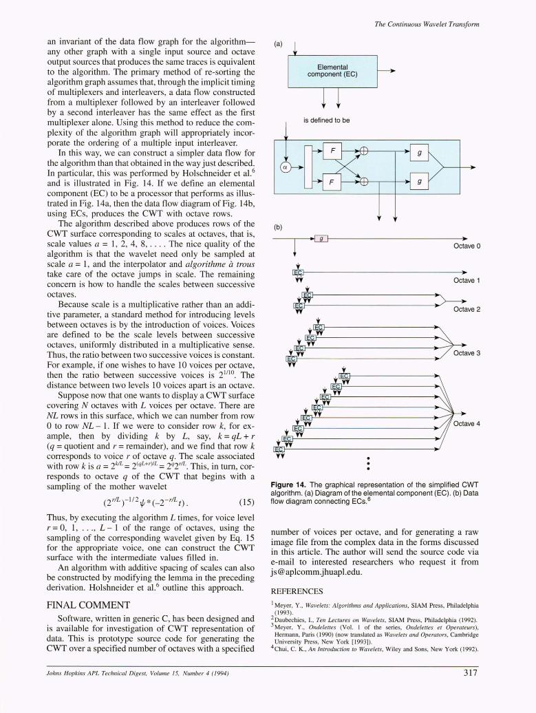
In this way, we can construct a simpler data flow for the algorithm than that obtained in the way just described. In particular, this was performed by Holschneider et a1.6

and is illustrated in Fig. 14. If we defIne an elemental component (EC) to be a processor that performs as illus­trated in Fig. 14a, then the data flow diagram of Fig. 14b, using ECs, produces the CWT with octave rows.

The algorithm described above produces rows of the CWT surface corresponding to scales at octaves, that is, scale values a = 1, 2, 4, 8, .... The nice quality of the algorithm is that the wavelet need only be sampled at scale a = 1, and the interpolator and algorithme a trous take care of the octave jumps in scale. The remaining concern is how to handle the scales between successive octaves.

Because scale is a multiplicative rather than an addi­tive parameter, a standard method for introducing levels between octaves is by the introduction of voices. Voices are defIned to be the scale levels between successive octaves, uniformly distributed in a multiplicative sense. Thus, the ratio between two successive voices is constant. For example, if one wishes to have 10 voices per octave, then the ratio between successive voices is 21110. The distance between two levels 10 voices apart is an octave.

Suppose now that one wants to display a CWT surface covering N octaves with L voices per octave. There are NL rows in this surface, which we can number from row o to row NL - 1. If we were to consider row k, for ex­ample, then by dividing k by L, say, k = qL + r (q = quotient and r = remainder), and we fInd that row k corresponds to voice r of octave q. The scale associated with row k is a = 2k/L = 2(qL+r)IL = 2Q2r1L. This, in tum, cor-responds to octave q of the CWT that begins with a sampling of the mother wavelet

(2rlL)-lI2l/;*(_2-rILt). (15)

Thus, by executing the algorithm L times, for voice level r = 0, 1, . .. , L - 1 of the range of octaves, using the sampling of the corresponding wavelet given by Eq. 15 for the appropriate voice, one can construct the CWT surface with the intermediate values fIlled in.

An algorithm with additive spacing of scales can also be constructed by modifying the lemma in the preceding derivation. Holshneider et a1.6 outline this approach.

FINAL COMMENT Software, written in generic C, has been designed and

is available for investigation of CWT representation of data. This is prototype source code for generating the CWT over a specifIed number of octaves with a specifIed

Johns Hopkins APL Technical Digest. Volume 15. Number 4 (1994)

(a)

(b)

I

Elemental component (EC)

is defined to be

-w

~ j

i •• rw

tW-W

t

The Continuous Wavelet Transform

~

Octave 0

~

Octave 1

:~ Octave 2

~~~3

tEC~~-------------~

EC~---------------~

'f · • •

Figure 14. The graphical representation of the simplified CWT algorithm. (a) Diagram of the elemental component (EC). (b) Data flow diagram connecting ECs.6

number of voices per octave, and for generating a raw image fIle from the complex data in the forms discussed in this article. The author will send the source code via e-mail to interested researchers who request it from [email protected].

REFERENCES

I Meyer, Y., Wavelets: Algorithms and Applications, SIAM Press, Philadelphia (1993).

2 Daubechies, I., Ten Lectures on Wavelets, SIAM Press, Philadelphia (1992) . 3 Meyer, Y., Ondelettes (Vol. I of the series, Ondelettes et Operateurs) ,

Hennann, Paris (1990) (now translated as Wavelets and Operators, Cambridge University Press, New York [1993]).

4 Chui, C. K. , An Introduction to Wavelets, Wiley and Sons, New York (1992).

317

J. Sadowsky

5Grossmann, A. , Kronland-Martinet, R. , and Morlet, J., "Reading and Under­standing Continuous Wavelet Transforms," in Wa velets: Time-Frequency Methods and Phase Space, J. Combes A. Grossmann, and Ph. Tchamitchian (eds.), Springer Verlag, ew York, pp. 2-21 (1989).

6 Holschneider, M. , Kronland-Martinet, R., Morlet, J. , and Tchamitchian, Ph. , "A Real-Time Algorithm for Signal Analysis with the Help of the Wavelet Transform," in Wa veleTS: Time-Frequency Methods and Phase Space, J. Combes, A. Grossmann, and Ph. Tchamitchian (ed .), Springer Verlag, New York, pp. 286-297 (1989).

THE AUTHOR

JOHN SADOWSKY received a B.S. in mathematics from The Johns Hopkins Univer ity and a Ph.D. in mathematics with a speciality in number theory from the University of Maryland. Before joining APL, he worked as a supervisor and Prin­cipal Scientist for the Systems Engi­neering and Development Corpora­tion and as a mathematician for the Social Security Administration and the Census Bureau. He joined APL's Research Center in 1989 and is currently the Assistant Supervisor of the Mathematics and Infonnation Science Group. In addition, since 1981 he has served on the adjunct

faculty for the Computer Science Program of the G.W.c. Whiting School of Engineering. Dr. Sadow ky' s current interests include signal process­ing, applied algebra and number theory, computational complexity, the design of algorithms, and sensory engineering.

318 fohns Hopkins APL Technical Digest. Volume 15, Number 4 (1994)