The conoidal ruled surfaces

The conoidal ruled surfaces(presented at the session of the class of mathematics and natural sciences on

October 7, 1982 by the member Walter Wunderlich)

Georg Glaeser

1 Introduction

In an earlier submission [2], the author presented “rotoidal ruled surfaces”;

which are traced by certain lines during the course of a “rotoidal motion”.

This spatial displacement is the superposition of two proportional rotations

about skew and orthogonal axes and was studied in detail [1] suggested by W.

Wunderlich.

The subject of the present note is the second special family of rotoidal

ruled surfaces, namely that one which is generated by a line that is parallel to

the moving axis, and therefore, yields conoidal ruled surfaces. These surfaces

posses an easy to be described striction curve, two types of self intersections,

and oscillation developables as circumscribed slope developables.

Again, special attention is paid to the assumption of a rational transmission

ratio n, since here algebraic ruled surfaces arise. The simplest case (n = 1)

yields oscillation ruled surfaces of degree 4 (Sturm type V) which are related

by affine transformations, having an ellipse for their striction curve. They can

be generated in two ways as rotoidal ruled surfaces, and moreover, they are

envelopes of one-parameter families of cones of revolution with parallel axes.

2 Rotoidal ruled surfaces with improper

directrix

Like in [2], let a > 0 denote the distance of the axes a1, a2, and let n > 0 be

the constant transmission ratio or the two rotations. Again, let the z-axis of a

Cartesian coordinate system (O;x, y, z) coincide with the fixed axis a1 and the

the “base plane” π : z = 0 may contain the gyrating axis a2. The y-axis shall

be parallel to a pose of the generating line g lying exactly above a2 (Fig. 1).

Then, using the rotation angle u about a1 (and hence nu about a2) and with

the parameter v on the generator, the rotoidal ruled surface Φn swept by g is

1

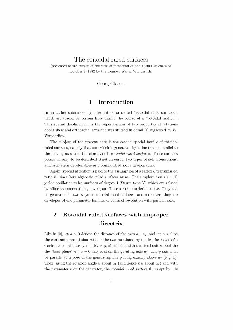
described by

x = (a+ b sinnu) cosu− v sinu,

y = (a+ b sinnu) sinu+ v cosu,

z = b cosnu.

(2.1)

Figure 1: Generation of a conoidal ruled surface

The straight generators g (u = const.) are consistently parallel to the base

plane π; the ruled surface Φn is, therefore, conoidal and contains the ideal line

of π as (improper) directrix.

With v = const., the equations (2.1) describe the orbits kn (“rotoids”) of

points undergoing the rotoidal motion located on Φn. Their periodic nature

(period δ = 2π/n) guarantees that the surface Φn can be transformed into

itself with rotations about the axis a1 through integer multiples of δ. Such a

rotoid k lies on a cyclic surface of revolution of degree 4 with axis a1. It is

generated by that circle that is traced by the corresponding point under the

rotation about a1 (Fig. 1). In the special case v = 0, the cyclic surface is a

torus with a meridian of radius b and the spine (circle) f : x2+y2 = a2, z = 0.

Since this torus is touched by the surface Φn along the rotoid kn (v = 0), it

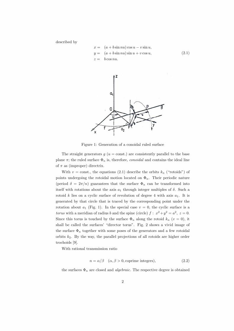
shall be called the surfaces’ “director torus”. Fig. 2 shows a vivid image of

the surface Φn together with some poses of the generators and a few rotoidal

orbits k2. By the way, the parallel projections of all rotoids are higher order

trochoids [9].

With rational transmission ratio

n = α/β (α, β > 0, coprime integers), (2.2)

the surfaces Φn are closed and algebraic. The respective degree is obtained

2

Figure 2: Conoidal ruled surface Φ2 of degree 6

as shown in [2], by computing the generators’ homogeneous Plucker coordinates

(with the help of the points v = 0 and v =∞)

p1 = − sinu, p4 = −b cosnu cosu,

p2 = cosu, p5 = −b cosnu sinu,

p3 = 0, p6 = a+ b sinnu.

(2.3)

Subsequently, we use the rational substitution

w = eiu/β (2.4)

which turns the Plucker coordinates into the form

p′1 = 2i(wα+2β − wα),

p′2 = 2(wα+2β + wα),

p′3 = 0,

p′4 = −b(w2α + 1)(w2β + 1),

p′5 = −ib(w2α + 1)(w2β − 1),

p′6 = 4awα+β − 2ib(w2α+β − wβ).

(2.5)

The intersection condition with an arbitrary line g yields with∑qip′i (and

constant qi) an algebraic equation in w from which the sought after degree of

the surface

N = 2(α+ β) (2.6)

can be read off.

3

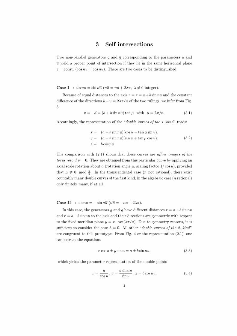
3 Self intersections

Two non-parallel generators g and g corresponding to the parameters u and

u yield a proper point of intersection if they lie in the same horizontal plane

z = const. (cosnu = cosnu). There are two cases to be distinguished.

Case I : sinnu = sinnu (nu = nu+ 2λπ, λ 6= 0 integer).

Because of equal distances to the axis r = r = a+ b sinnu and the constant

difference of the directions u−u = 2λπ/n of the two rulings, we infer from Fig.

3:

v = −d = (a+ b sinnu) tanµ with µ = λπ/n. (3.1)

Accordingly, the representation of the “double curves of the 1. kind” reads:

x = (a+ b sinnu)(cosu− tanµ sinu),

y = (a+ b sinnu)(sinu+ tanµ cosu),

z = b cosnu.

(3.2)

The comparison with (2.1) shows that these curves are affine images of the

torus rotoid v = 0. They are obtained from this particular curve by applying an

axial scale rotation about a (rotation angle µ, scaling factor 1/ cosu), provided

that µ 6≡ 0 mod π2 . In the transcendental case (n not rational), there exist

countably many double curves of the first kind, in the algebraic case (n rational)

only finitely many, if at all.

Case II : sinnu = − sinnu (nu = −nu+ 2λπ).

In this case, the generators g and g have different distances r = a+ b sinnu

and r = a− b sinnu to the axis and their directions are symmetric with respect

to the fixed meridian plane y = x · tan(λπ/n): Due to symmetry reasons, it is

sufficient to consider the case λ = 0. All other “double curves of the 2. kind”

are congruent to this prototype. From Fig. 4 or the representation (2.1), one

can extract the equations

x cosu± y sinu = a± b sinnu, (3.3)

which yields the parameter representation of the double points

x =a

cosu, y =

b sinnu

sinu, z = b cosnu. (3.4)

4

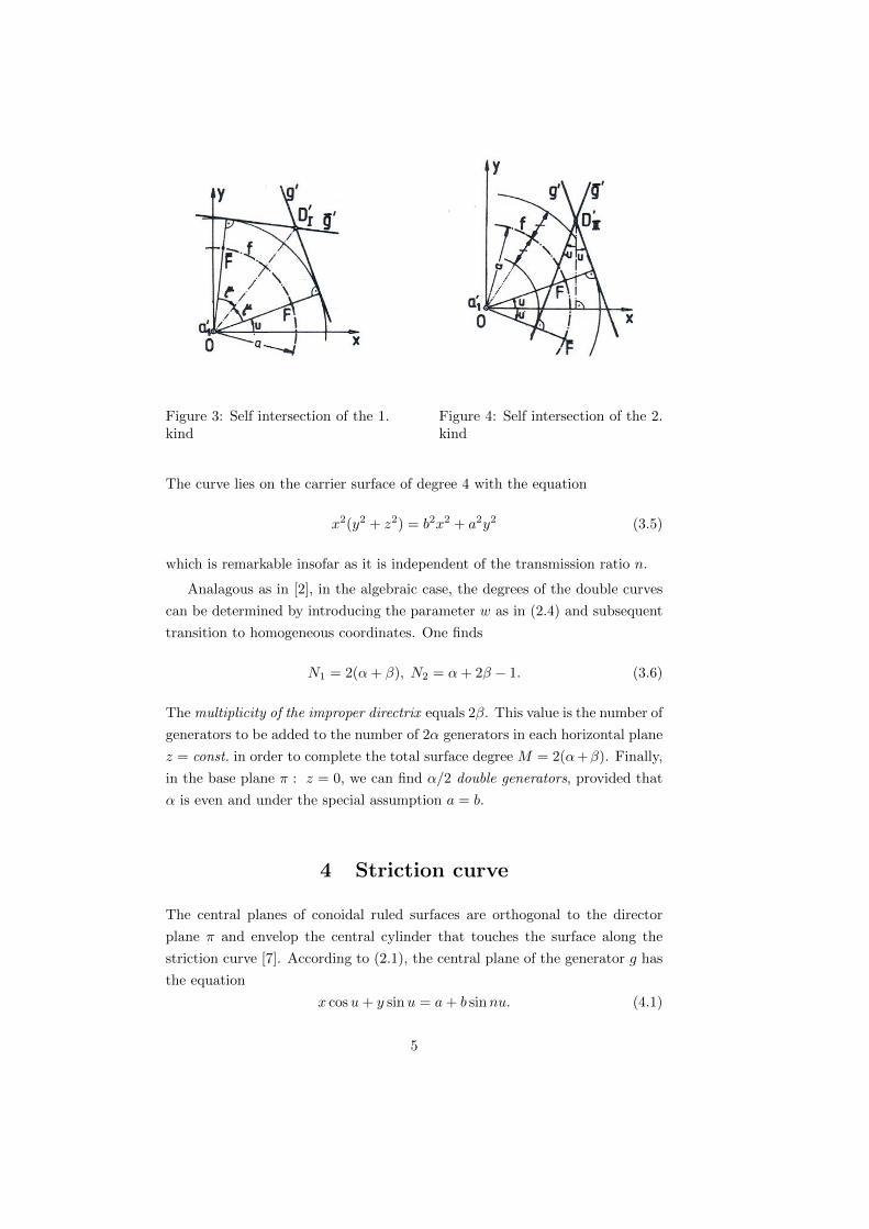
Figure 3: Self intersection of the 1.kind

Figure 4: Self intersection of the 2.kind

The curve lies on the carrier surface of degree 4 with the equation

x2(y2 + z2) = b2x2 + a2y2 (3.5)

which is remarkable insofar as it is independent of the transmission ratio n.

Analagous as in [2], in the algebraic case, the degrees of the double curves

can be determined by introducing the parameter w as in (2.4) and subsequent

transition to homogeneous coordinates. One finds

N1 = 2(α+ β), N2 = α+ 2β − 1. (3.6)

The multiplicity of the improper directrix equals 2β. This value is the number of

generators to be added to the number of 2α generators in each horizontal plane

z = const. in order to complete the total surface degree M = 2(α+β). Finally,

in the base plane π : z = 0, we can find α/2 double generators, provided that

α is even and under the special assumption a = b.

4 Striction curve

The central planes of conoidal ruled surfaces are orthogonal to the director

plane π and envelop the central cylinder that touches the surface along the

striction curve [7]. According to (2.1), the central plane of the generator g has

the equation

x cosu+ y sinu = a+ b sinnu. (4.1)

5

Its contact point with the surface Φn lies in the plane obtained by differentiation

− x sinu+ y cosu = nb cosnu, (4.2)

and therefore, it has the coordinates

x = (a+ b sinnu) cosu− nb cosnu sinu,

y = (a+ b sinnu) sinu+ nb cosnu cosu,

z = b cosnu.

The latter equations describe the (proper) striction curve s of Φn, which is,

therefore, characterized by

v = nb cosnu, (4.3)

as can be seen by comparing with (2.1).

The top view s′ of the striction curve – which is at the same time the contour

of the surface with respect to the orthogonal projection onto the base plane [7]

– has the complex representation

x+ iy = a · eiu +ib

2[(1 + n)e(1−n)iu − (1− n)e(1+n)iu]. (4.4)

If n 6= 1, it is a cycloid of order 3 with the characteristic (1−n) : 1 : (1+n) [9].

It is an involute of the cycloids with characteristic (1− n) : (1 + n) enveloped

by the lines (4.2), i.e., of an epicycloid if n < 1 or a hypocycloid if n > 1. In

the limit case n = 1 the curve s′ is a circle (cf. Section 5). Except this special

case, the degree of the striction curve equals the degree N of the surface 2.6.

The distribution parameter of a generator g of the surface Φn can immedi-

ately be obtained as the limit of the quotient of the distance and the direction

difference of two neighboring generators, and therefore, it equals

d = dz/du = −nb sinnu. (4.5)

From this, one can immediately infer that the proper torsal generators (d = 0)

of the surface are located in the horizontal planes z = ±b which touch the

surface along the entire generators. The corresponding cuspidal points (v =

±nb) are the intersections of the striction curve s and the double curve of the

2. kind.

With w = 0 and w = ∞ and according to (2.5), we find two isotropic

improper generators (0 : 0 : 0 : 1 : ±i : 0) which are cylindrical because of

d = ∞ and touch the absolute conic. According to [5, 7], they have to be

counted as improper components of the striction curve.

6

5 Circumscribed slope developables

All tangent planes τ of the surface Φn, which enclose a constant angle γ with the

base plane π envelop a slope developable Γ circumscribed to Φn. The direction

vector of the surface normal is computed from the partial derivatives of the

position vector (2.1) of the surface points x = (x, y, z)T, i.e.,

xu =

(nb cosnu− v) cosu− (a+ b sinnu) sinu

(nb cosnu− v) sinu+ (a+ b sinnu) cosu

(−nb sinnu)

, xv =

− sinu

cosu

0

(5.1)

by computing the exterior product

n = xu × xv =

−nb sinnu cosu

−nb sinnu sinu

−nb cosnu+ v

(5.2)

It encloses the angle γ with the z-direction if

v = nb(cosnu+m sinnu) with m = cotγ (5.3)

Inserting this value into the equation of the surface (2.1) yields the rep-

resentation of the curve c of contact of the surface Φn and the circumscribed

slope developable Γ:

x = (a+ b sinnu) cosu− nb(cosnu+m sinnu) sinu,

y = (a+ b sinnu) sinu+ nb(cosnu+m sinnu) cosu,

z = b cosnu.

(5.4)

This curve c can be interpreted as isophote of the surface Φn under parallel

lighting in the direction of the axis a1 and appears in the top-view as a cycloidal

curve of order 3 and characteristic (1 − n) : 1 : (1 + n). As a limit case with

m = 0, the striction curve s from (4.3) is obtained.

The tangent plane τ that generates the slope developable has the normal

vector (cosu, sinu, cotγ)T and, by virtue of (2.1), the equation

x cosu+ y sinu+mz = a+ b sinnu+mb cosnu. (5.5)

Observing the intersection point with the fixed axis a1 (x = y = 0), one

learns that the sequence of poses of the plane τ is obtained by the action of the

uniform rotation about a1 and the superposed harmonic oscillation along a with

frequency n. The slope developable Γ is, therefore, a oscillation developable.

7

According to W. Kautny [3], the curve of regression is a curve of constant slope

on a quadric of revolution whose axis is parallel to a1, as long as n 6= 1.

Using the first two derivatives of the planes’ equation 5.5, i.e.,

−x sinu+ y cosu = nb(cosnu−m sinnu),

x cosu+ y sinu = n2b(sinnu+m cosnu),(5.6)

the mentioned curve of regression can be written in terms of complex coordi-

nates as

x+ iy = nb2 [(m− i)(n− 1)e(1+n)iu + (m+ i)(n+ 1)e(1−n)iu],

mz = a+ b(1− n2)(sinnu+m cosnu).(5.7)

It appears as an epicycloid in the top-view if n < 1 and as a hypocycloid if

n > 1. The corresponding carrier quadric which is described by

x2 + y2

n2+

(mz − a)2

1− n2= (m2 + 1)b2 (5.8)

is either an ellipsoid of revolution or a one-sheeted hyperboloid of revolution.

The limit case to be postponed with n = 1 is treated in the next section.

6 Conoidal ruled surfaces of degree 4

With n = 1 (α = β = 1) and according to (2.6), we obtain biquadratic ruled

surfaces Φ1. According to Section 3, their self intersections consist of the

improper directrix with multiplicity 2 and the equilateral hyperbola

x = a/ cosu, y = b, z = b cosu, (6.1)

and thus, this surface is of Sturm type V [7]. Eliminating w and v from the

representation (2.1) written with n = 1 yields the implicit equation

b2(xz − ab)2 + (y − b)2(z2 − b2) = 0 (6.2)

of the surface from which we can see that any two surfaces Φ1 are related by

an affine transformation and are symmetric with respect to the carrier plane

y = b of the double hyperbola (6.1).

The striction curve s of Φ1 is an ellipse according to (4.3)

x = a cosu, y = a sinu+ b, z = b cosu. (6.3)

The latter is the intersection of the plane bx = az with the cylinder of revolution

8

∆ : a2 + (y − b)2 = a2 which is the central cylinder.

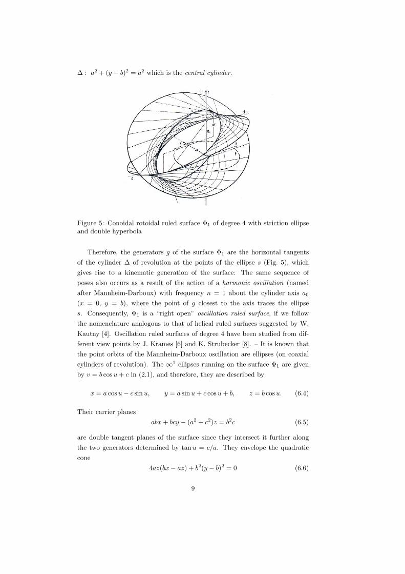
Figure 5: Conoidal rotoidal ruled surface Φ1 of degree 4 with striction ellipseand double hyperbola

Therefore, the generators g of the surface Φ1 are the horizontal tangents

of the cylinder ∆ of revolution at the points of the ellipse s (Fig. 5), which

gives rise to a kinematic generation of the surface: The same sequence of

poses also occurs as a result of the action of a harmonic oscillation (named

after Mannheim-Darboux) with frequency n = 1 about the cylinder axis a0

(x = 0, y = b), where the point of g closest to the axis traces the ellipse

s. Consequently, Φ1 is a “right open” oscillation ruled surface, if we follow

the nomenclature analogous to that of helical ruled surfaces suggested by W.

Kautny [4]. Oscillation ruled surfaces of degree 4 have been studied from dif-

ferent view points by J. Krames [6] and K. Strubecker [8]. – It is known that

the point orbits of the Mannheim-Darboux oscillation are ellipses (on coaxial

cylinders of revolution). The ∞1 ellipses running on the surface Φ1 are given

by v = b cosu+ c in (2.1), and therefore, they are described by

x = a cosu− c sinu, y = a sinu+ c cosu+ b, z = b cosu. (6.4)

Their carrier planes

abx+ bcy − (a2 + c2)z = b2c (6.5)

are double tangent planes of the surface since they intersect it further along

the two generators determined by tanu = c/a. They envelope the quadratic

cone

4az(bx− az) + b2(y − b)2 = 0 (6.6)

9

which (besides the improper directrix) is the proper component of the double

developable of Φ1.

The already mentioned plane of symmetry y = b, whose existence becomes

immediately evident by considering the generation of the surface via the har-

monic oscillation, allows us to generate the surface Φ1 as a rotoidal ruled sur-

face in two ways: Besides the initial rotoidal motion with the fixed axis a1

(x = y = 0) and the transmission ratio n = 1, we can use the motion with

the axis a1 (x = 0, y = 2b) and the transmission ratio n = −1. Consequently,

the surface Φ1 carries two symmetric families of rotoids (of degree 4). They

are given by inserting v = const. or v− 2b cosu = const. into (2.1). Especially,

v = 0 and v = 2b cosu yield two congruent torus rotoids along which the sur-

face Φ1 is touched by two congruent director tori (Section 2). Each generator

of the surface Φ1 touches one torus from the outside and the other from the

inside.

The slope developables circumscribed to the surfaces mentioned in Section 5

deserve special attention. According to (5.5), they are cones of revolution with

axes parallel to a1. Their vertices have the coordinates x = mb, y = b, z = a/m,

and therefore, they exhaust the double hyperbola (6.1). Consequently, the

surface Φ1 can also be obtained as the envelope of the ∞1 cones of constant

slope

(x−mb)2 + (y − b)2 = (mz − a)2 (6.7)

where m is the parameter in the family.

The curve of contact of such a cone (isophote of Φ1) is the limit shape of the

intersection curve of two infinitely close cones of revolution, and therefor, it is a

spherical quartic that touches the absolute conic twice and has a double point

in the cone’s vertex. According to (5.4), these isophotes appear as Pascal’s

limacons in the top view, while they are mapped to doubly covered parabolas

(of a pencil) in orthogonal projections onto the plane of symmetry y = b.

References

[1] Glaeser, G.: Uber die aus zwei gleichformigen Drehungen um rechtwinke-

lig kreuzende Achsen zusammengesetzte Raumbewegung. PhD thesis, TU

Wien, 1980.

[2] Glaeser, G.: Uber die Rotoidenwendelflachen. Sb. d. Osterr. Akad. d.

Wiss. 190 (1981), 285–302.

[3] Kautny, W.: Zur Geometrie des harmonischen Umschwungs. Monatsh.

Math. 60 (1956), 66–82.

10

[4] Kautny, W.: Uber die durch harmonischen Umschwung erzeugbaren

Strahlflachen. Monatsh. Math. 63 (1959), 169–188.

[5] Krames, J.: Uber das Zerfallen der Striktionslinie von Regelflachen. Sb.

d. Osterr. Akad. d. Wiss. 135 (1926), 227–269.

[6] Krames, J.: Zur aufrechten Ellipsenbewegung des Raumes. Monatsh.

Math. Phys. 46 (1937), 38–50. — Uber die durch aufrechte Ellipsenbe-

wegung erzeugbaren Regelflachen Θ. Jber. DMV 50 (1940), 58–65.

[7] M uller, E. and Krames, J.: Konstruktive Behandlung der Regelflachen

(Vorlesungen uber Darstellende Geometrie, Bd. III). Leipzig/Wien 1937.

[8] Strubecker, K.: Komplexe Geometrie und aufrechte Ellipsenbewegung.

Jber. DMV 50 (1940), 43–58.

[9] Wunderlich, W.: Hohere Radlinien. Osterr. Ingen.-Archiv 1 (1947), 277–

296.

11