The Concept of a Stare-Mode Astrometric Space Mission

arX

iv:a

stro

-ph/

0608

286v

1 1

4 A

ug 2

006

accepted by PASP, October 2006 issue

The concept of a stare-mode astrometric space mission

N. Zacharias and B. Dorland

U.S. Naval Observatory, Washington, DC 20392,

[email protected], [email protected]

ABSTRACT

The concept of a stare-mode astrometric space mission is introduced. The

traditionally accepted mode of operation for a mapping astrometric space mission

is that of a continuously scanning satellite, like the successful Hipparcos and

planned Gaia missions. With the advent of astrometry missions mapping out

stars to 20th magnitude, the stare-mode becomes competitive. A stare-mode of

operation has several advantages over a scanning missions if absolute parallax

and throughput issues can be successfully addressed. Requirements for a stare-

mode operation are outlined. The mission precision for a stare-mode astrometric

mission is derived as a function of instrumental parameters with examples given.

The stare-mode concept has been accepted as baseline for the NASA roadmap

study of the Origins Billions Star Survey (OBSS) mission and the Milli-arcsecond

Pathfinder Survey (MAPS) micro-satellite proposed project.

Subject headings: astrometry — space vehicles — techniques: miscellaneous

1. Introduction

The current paradigm for a mapping, astrometric space mission is a scanning satellite

with 2 fields of view (FOV) which are separated by a large angle of ≈ 50◦ to 100◦. This

concept was first introduced by P. Lacroute (Lacroute 1982). The 2 FOV are imaged onto

the same focal plane, thus relative position measures of stellar images in the focal plane

allow wide-angle measures on the sky. This observing strategy leads to a well conditioned

least-squares problem to solve for absolute parallaxes. For any small area in the sky the

parallax factor (van de Kamp 1967) is about the same, leading to large correlations in a

global solution for absolute parallaxes based on stellar, all-sky observations of small angle

astrometric measures alone.

– 2 –

This concept of 2 FOV separated by a “basic angle” worked very well for the ESA

Hipparcos mission (ESA 1997). This concept has been adopted also for the planned ESA

Gaia mission (Gaia report 2000), as well as the canceled FAME mission (Johnston 2003) and

the unfunded DIVA (Roser 2000) and AMEX (Gaume & Johnston 2003) missions. Another

advantage of this concept is the almost 100% efficiency in data collection with continuous

observations in time-delayed integration (TDI) mode using charge-coupled devices (CCDs).

Together with the success of the Hipparcos mission, the scanning concept has been adopted as

“the optimal” concept for a mapping astrometric mission.1 However, going to much higher

accuracies and fainter limiting magnitudes with access to galaxies and quasars justifies a

second look at the basic operation principle and possible alternatives.

The stare-mode concept for an all-sky, mapping, astrometric space mission is presented

here, which requires only a single FOV and operates differentially. This is contrary to the

quasi-absolute, large-angle measure principle using 2 FOV with a scanning mission. A stare-

mode operation with 2 FOV is technically feasible. However, this approach would avoid only

some of the issues raised here for a scanning mission and is not discussed further.

In section 2 the disadvantages of scanning, astrometric space missions are presented and

in section 3 the stare-mode concept is presented as an alternative to overcome these problems,

stressing the requirements which need to be meet in order to be a viable option. In section 4

mission precision and other relevant mission parameters are derived from instrumental and

basic input parameters. Section 5 discusses some realistic examples for small and large-scale

astrometric missions based on this stare-mode concept. The Origins Billions Star Survey,

OBSS (Johnston et al. 2004) study adopted as baseline the proposed stare-mode operation

principle. OBSS is a NASA sponsored investigation for NASA roadmap planning. The OBSS

study report was submitted in May 2005 (Johnston et al. 2005), and more details are given

elsewhere (Johnston et al. 2006).

2. Disadvantages of a scanning astrometric mission

The main issues with a scanning astrometric mission like Hipparcos and Gaia are:

Basic angle stability. In the 1 mas regime (Hipparcos) the basic angle stability was al-

ready technologically challenging. For 10 µas this becomes a major cost driver and

1The Space Interferometry Mission (SIM) is also a dedicated, astrometric mission; however, it operates

on a totally different concept (interferometry) and can observe only a very limited number of pre-selected

targets.

– 3 –

primary source of systematic errors. For example the Gaia design (Gaia report 2000)

requires passive temperature stability in the micro-Kelvin regime and an active metrol-

ogy system.

2 apertures separated by large angle. This has the advantage of direct, wide-angle mea-

surements, but on the other hand becomes a problem with respect to image confusion

and crowding in the focal plane and instrument complexity with the tough engineering

requirement of having no significant beam walk to make use of this concept as intended.

The complexity of a beam-splitter hardware is costly.

CCD vs. CMOS. The scanning concept relies on driving focal plane detectors in TDI

mode, which can be accomplished only with CCDs. Complementary Metal Oxide

Semiconductor (CMOS) detectors, (or hybrid detectors) which show promise for future

applications, may be better suited for space applications, being radiation hard. In ad-

dition, CMOS pixels don’t spill charge (blooming) and thus are inherently better suited

for bright star astrometric observations and for spanning a very large dynamic range,

even when small pixel sizes are considered. Current CCD technology supports various

anti-blooming features. However, the most effective, lateral anti-blooming becomes

increasingly problematic for CCDs as the pixel size decreases, effectively becoming

impractical at the 8 µm size.

Scanning restrictions. The scanning mission is limited to a specific scanning law. No

target of opportunity can be observed. Also, the integration time is fixed (optimized

for uniform scanning speed), and typically relatively short (i.e. a few seconds) due to

other constraints, forcing the mission to use a large aperture to reach faint limiting

magnitudes. Slower scanning is undesirable for satellite stability and other reasons.

Large apertures drive focal length, mass and cost and make access to bright stars

problematic. The scanning law and the Sun exclusion angle lead to an uneven sky

coverage with a typical average mission precision variation of astrometric parameters

by a factor of 2 as a function of ecliptic latitude. No specific target areas can be

observed with other precision than dictated by the scanning law. The temporal cadence

of observations has no flexibility.

Image smearing. The spacecraft angular momentum vector needs to precess to produce

an all-sky survey. The continuous precession results in image smearing. Remaining

differential distortions over the field of view add to image smearing. Elongated, or

generally asymmetric image profiles increase the astrometric errors, random as well as

systematic errors.

Jitter. Small non-uniformities of the scanning (spacecraft jitter) cause changes in the image

– 4 –

profiles as a function of time. The TDI mode does not integrate all stars in a given field

simultaneously, thus different stars observed almost at the same epoch (same FOV),

are affected differently, leading to positional offsets which need to be modeled or cause

additional random and systematic errors.

1-dim data. The scanning operation gives only 1-dimensional measures of high precision.

This has some advantages (i.e. simple profile fit) but has significant disadvantages in

the later stages of the data reduction and global astrometric re-construction (error

propagation issues, mixing with instrumental effects, attitude control). Also for many

applications (parallaxes, planet detections) the 1-dim observations will be quite often

(near 50%) along the “wrong axis”, while 2-dim data gives results for any projection

angle for any single observation.

Downlink. It is difficult to use a steerable, high gain antenna (HGA) to achieve a large

downlink rate from an L2 orbit. A spinning satellite, in order to achieve comparable

data rates (≈ 30 Mbps), must either be positioned close to Earth or employ a dedicated

relay satellite equipped with a direction HGA at significant additional cost to the

program. A stare-mode satellite could be equipped with a HGA.

3. The stare-mode concept

For a stare-mode mission (with a single FOV) to be considered as a viable alternative

to the scanning satellite concept, 2 basic issues need to be addressed and solved:

1. Global astrometric accuracy from stitching together small, overlapping fields, without

the advantage of direct large angle measurements (particularly for absolute parallax

determination).

2. Overhead time (observing efficiency) for setting to the next field needs to be short

including actual slew of spacecraft, settling time, guide star acquisition and detector

read out time.

3.1. Global astrometry with block adjustment techniques

3.1.1. Traditional, ground-based technique

The stare-mode idea presented here follows closely the traditional, photographic as-

trometry survey principle. The telescope is pointed at a field of view and all stars in the

– 5 –

focal plane are integrated simultaneously while the pointing and field orientation angle are

kept constant with the help of 2 or more guide stars. Then the FOV is shifted and the next

field is exposed. Consecutive FOV are overlapped by typically 25 to 50% in area. A zonal

pattern of the sky is covered within a short period of time which is eventually supplemented

by similar adjacent, overlapping observations to cover the entire sky.

This pattern of overlapping fields allow for a block adjustment (BA) (Eichhorn 1960; de

Vegt & Ebner 1974; Googe, Eichhorn & Lukac 1970), in which the astrometric and instru-

mental parameters (“plate constants”) are estimated at the same time in a single, rigorous,

non-linear, least-squares adjustment. Any applicable reference star catalog will be sufficient

for an initial reduction of the data to get approximate starting values for the linearized BA

procedure, which converges typically in a single iteration step. The problem is rank deficient;

an external orientation of the global coordinate system needs to be provided2. Usually the

then available “best” celestial reference frame is chosen for this external orientation to be

consistent with the previous realization of such a system.

Alternatively to the BA reductions an iterative conventional adjustment (ICA) scheme

can be used to perform the global reductions. A classical “single plate” adjustment gives

improved positions for reference and selected field stars on a frame-by-frame basis. For

individual stars then data are combined to obtain mean position, proper motion and parallax,

from all overlapping fields and from different epochs. These improved data are fed into the

next iteration to repeat the adjustment. The ICA scheme converges to a consistent, global

catalog up to the accuracy limits of the input x, y-coordinates on a reference system which

is represented by the average of all the original reference catalog star coordinates (external

system orientation and rotation). Both the BA and ICA approach give equivalent results

(Benevides-Soares & Teixeira 1992). The BA approach is conceptually “cleaner” than the

ICA but takes a hugh amount of computer resources. Contrary to just the single-step classical

“plate reduction”, the BA and ICA concepts explicitely utilize the astrometric information

(same star on different exposures has only 1 set of astrometric parameters) from overlapping

fields, involving all (suitable) stars in the reductions, not just the few reference stars.

The BA concept has been successfully applied for a few cases (Fuhrmann 1979; Zacharias 1988)

and has been studied with simulations (Zacharias 1992). Important to realize is that with

a BA type reduction the scale and orientation (roll angle) parameters of each individual

exposure is determined very precisely. If there is for some reason a jump in scale between

exposures or a very small drift, it will not affect the astrometric results of the reductions.

Scale and orientation are overall very few parameters in a well conditioned system of obser-

2The same is true also for a scanning mission.

– 6 –

vation equations when dealing with many star images per exposure.

Although these applications so far dealt with positions only, the formal extension of

the principle and algorithm to include proper motions and parallaxes is straightforward.

However, deriving absolute parallaxes and proper motions from small angle measures (ICA

or BA) deserves some elaboration (see below).

3.1.2. Difference between SIM and astrograph-type observations

The Space Interferometry Mission (SIM) (Unwin & Shao 2000) has only a single field

of regard (FOR); however, this FOR is relatively large (15◦). Rigorous simulations

(Makarov & Milman 2005) have shown that the mission goals for all 5 astrometric parameters

(position, proper motion and parallax) can be achieved, although the least-squares system

is not well conditioned, at least if just stars are used for the astrometric grid as originally

planned. Recent simulations (Makarov et al. 2006) show that by including even a small

number of extragalactic, fixed fiducial points (≈ 25 QSOs) the absolute errors in parallax

become significantly smaller (about factor of 2).

It is important to keep in mind that SIM observations are fundamentally different than

the astrograph-type mapping observations suggested here. SIM does obtain (relatively) large-

angle, absolute measures. However, SIM observes only 1-dimensional, angular separations

between 2 targets at a time and a global grid needs to be stiched together by these quasi ab-

solute angle measures, including all instrumental parameters before any catalog of positions

and motions can be established. A single astrograph-type observation yields differential,

2-dimensional positions for thousands of targets simultaneously with a minimal number of

instrumental parameters. Relative proper motions can be derived from astrograph-type

observations of the same field at 2 or more different epochs, even without any overlap to

adjacent fields, see e.g. the Northern and Southern Proper Motion Surveys, NPM, SPM

(Klemola et al. 1994; Platais et al. 1997).

3.1.3. Will the stare-mode reductions work for global, astrometric, space missions?

Block adjustment procedures in ground-based, traditional, photographic astrometry can

successfully be applied even in the case of very few reference objects (Zacharias 1992). The

BA technique does not work very well for a zonal pattern (fields along a narrow strip around

the sky) in the presence of systematic errors, but is well conditioned for a hemisphere or

all-sky coverage due to the many inherent “closure conditions” (after going around the sky in

– 7 –

a circle, the same stars are mapped, forcing to the same positions, give or take parallax/PM

effects). A narrow zone has closure only along 1 axis, while the hemisphere or all-sky case

is much ”stiffer” with closures in 2 dimensions. Imagine a zone of few degrees width around

the equator. Coordinates along RA are well constraint due to the closure at 0/24 hours RA.

However the star positions could easily have systematic errors along declination, for example

as a function of RA. With the entire hemisphere covered, there are multiple constraints

reaching from one side over the pole to the other side to ”fix” zonal errors.

Critical for the success of a BA or ICA approach, besides a hemisphere or all-sky coverage

are 4 issues:

1. Sufficient overlap between adjacent fields.

2. Sufficient number of link stars in overlapping frames.

3. Fiducial points for absolute parallax and proper motion determination.

4. High instrumental stability of higher order variations (mapping model).

The first item is easily accommodated. The stare-mode operation allows for a flexible

cadence to observe adjacent fields with overlaps as required.

The second item requires a large number of stars per unit area in the sky. This typically

becomes feasible with a faint limiting magnitude of the instrument. For a Hipparcos-type

mission this actually would have been a problem but it is not an issue for a Gaia or OBSS

type mission. For a well conditioned system, the mission precision, σm (mean astrometric

errors for a given target object, averaged over all observations of that target during the

lifetime of the mission) will approach the σm = σsmp/√

nt limit, with the single measure

error σsmp and the number of observations, nt, per target (per coordinate).

Simulations with only a 4-fold overlap pattern of a hemisphere using a small FOV of

4◦ and only about 200,000 stars lead to a well conditioned system with the actual σm being

larger than the square-root-n limit by only about a factor of 1.04 (Zacharias 1992) for star

positions.

Random errors of individual stellar position observations can lead to a zero-point offset

of an entire field of about σsmp/√

ns, with ns being the number of (well exposed) stars in that

field of view. If ns is significantly larger than nt, this zero-point offset of a field (i.e. zonal

error) is likely to be smaller than the envisioned mean mission errors. In the example cases

given below this requirement is met, and the BA reduction procedure likely will give the

– 8 –

expected performance. Detailed simulations with the specific mission parameters for the

OBSS case are planned for a phase A study.

The third requirement can be met by observations of quasars and compact galaxies.

As soon as the limiting magnitude of the instrument can access a significant number of

these extragalactic sources they provide absolute reference points for parallaxes and proper

motions. This concept is proven even for not-much-overlapping, differential, ground-based

observations, for example by the Northern and Southern Proper Motion projects, NPM and

SPM (Klemola et al. 1994; Platais et al. 1997). Again, this was not an option for Hipparcos

but is not an issue for either OBSS or Gaia, which reach limiting magnitudes of 21 and

20, respectively. The zone of avoidance, i.e. the galactic plane with high extinction areas

is a comparatively small area in the sky for a global program and the BA technique of

linking all FOV should be able to “bridge” those areas (pending further simulations to verify

this assumption). Furthermore, some optical counterparts of quasars have been confirmed at

very low galactic latitudes (Zacharias & Zacharias 2005), and only a small number of fiducial

points are required to set the zero-point for absolute parallaxes and proper motions.

The last item needs engineering attention in any case, 1 or 2 FOV, scanning or stare-

mode observations. However, for the 2 FOV, large-angle measure approach, challenging

basic-angle stability/monitoring requirements have to be added. The stare-mode option has

the big advantage of being totally differential. Even a change in scale from one FOV to

the next is easy to handle; only a few instrumental parameters like zero-point, scale and

orientation per FOV contrast the large number of observations (individual x,y data of stel-

lar images observed simultaneously) and the large number of overlap connections (adjacent

fields, number of repeats of all-sky pattern). This leads to relatively low requirements on

thermal gradients etc. in the instrument design with significant cost benefits as compared to

a quasi-absolute, large-angle measure approach. The only requirement is that higher order

mapping terms (field distortion pattern etc.) are “calibrated out” and a simple mapping

model must describe the individual frames in the final BA (after an iteration and calibra-

tion). If too many parameters and changing calibration values over short periods of time are

required, the global astrometry would suffer from significant error propagation losses.

3.2. Overhead

The stare-mode operation is potentially more inefficient than a spinning observatory

that employs TDI-mode observing. There are 2 primary sources of inefficiency: first, during

step-stare observing, the detectors must be read out. The readout period must be sufficiently

long to permit low read noise from the detector amplifiers and the readout electronics. Using

– 9 –

standard CCD technology, no photons can be collected during readout, making the readout

period essentially dead time in terms of integration. If, on the other hand, active pixel

sensor (APS) detector technology such as CMOS or CMOS-Hybrid sensors are used, pixels

are read out while integration continues, eliminating this source of inefficiency. APS detector

technology has the added benefit of supporting electronic shuttering, eliminating the need

for a mechanical shutter.

The second source of overhead is repositioning of the field of view after a field has been

observed. During the repositioning of the field of view (and during any subsequent settling

period of the structure), astrometric observations cannot be taken. The overhead can be

minimized by overlapping the read-out time with the reposition and settle time. However,

it is important to remember that a scanning mission observes only 1-dim data while the

stare-mode approach obtains 2-dim data simultaneously, thus starting out with a factor of

2 advantage during the time of photon collection.

A somewhat lower efficiency is not necessarily a bad thing for astrometry, if a higher

astrometric quality (smaller systematic errors) is obtained. All dedicated astrometric instru-

ments lose photons. Hipparcos utilized a modulating grid in the focal plane to observe a

star at a time, disregarding all the other targets which would have been accessible simulta-

neously. Astrographs use narrow filters and sometimes grating images, reducing the limiting

magnitude. Note, the spinning observatory loses efficiency in other places: unfavorable error

propagations with 1-dim observations when scans do not intersect near orthogonal and 1-dim

observations at a time.

Assuming an operation principle similar to HST which takes minutes to re-position

to the next FOV, the stare-mode astrometric mission would not be an option. Current

technology provides a couple of different solutions that lead to acceptable overhead times.

For small apertures (≤ 0.5 m) one can envision a moveable, full-aperture scan mirror that,

for example, rotates in half-degree increments so as to access a large arc (100 to 360 degrees)

for a step-stare instrument without requiring reorientation of the observatory. Such an

instrument has been discussed and appears feasible (K. Aaron, priv. comm.). As the aperture

increases, however, the size and mass of the support structure, and method of moving the

full aperture flat scanning mirror become increasingly problematic. At 1.5 m, a 45 degree

inclination of the scan mirror with respect to the optical axis would result in a 2.2 m flat.

This optical element must be properly stowed in the available fairing, must be deployed

on-orbit, the torsional effects on the optical structure due to rotation of the mirror must be

compensated, and a non-trivial mechanism deployed in order to move the large flat. Moving

the entire observatory seems more practical at least for large aperture stare-mode missions,

and likely even for small apertures (Dorland & Zacharias 2005). This would not be feasible

– 10 –

using reaction wheel technology, with slew and settle times of order 100 seconds per field,

and a resultant ≈ 10% observing efficiency. Control Moment Gyros (CMGs), or constant

speed wheels, provide much higher torques, have proved space heritage, and are commercial,

off-the-shelf items.

A dead-time (no photon collection) of about 50% of the time over the entire mission can

be considered as very efficient as compared to a scanning operation (see above 1-dim versus

2-dim observations). The number of collected photons, leaving all other mission parameters

the same would be less in the stare-mode option, but the number of individual observations

(stellar image coordinates) would be the same for both cases.

It should be noted that the stare-mode concept, with its constant readout and slew

times, is naturally more efficient when taking long exposures. A 100 sec exposure with a 10

sec overhead results in 90% observing efficiency, for example. When combined with the fact

that longer exposures using similar optics and detector performance result in a fainter noise

floor, the stare-mode observing mode would appear to be more naturally suited to fewer,

deeper exposures vs. the scanning observing mode.

The loss due to overhead time in a stare-mode mission can be compensated by increasing

the size of the focal plane array (see also section 4), at the expense of a moderately reduced

aperture. The stare-mode still can go deeper (longer integration time) and is not restricted

by the downlink rate (directed beam antenna is possible) as e.g. the FAME mission concept

was. With selected field observing, possible if desired in stare-mode, denser areas can be

targeted more often which dramatically enhances the ratio of observing stars versus observing

empty space.

3.3. Stare-mode operational details

Operation of the envisioned stare-mode astrometric mission would go as follows. The

telescope slews to a new field, locks on at least 2 guide stars, settles and starts tracking.

Then the longer of 2 exposures begins, followed by a read-out of the detector array, while

the pointing of the telescope is still fixed with guide trackers running. The second, shorter

exposure is taken. While the detector array reads out again, the guiders are disengaged and

the telescope moves to the next, adjacent field.

The 2 exposure times of different duration (e.g. factor of 10) allow coverage of a large dy-

namic range and also are good astrometric practice to check on possible magnitude-dependent

systematic errors. More than 2 exposures per pointing can be observed if required, e.g. with

different filters, if a design including refractive elements is favored.

– 11 –

On-board processing would include the raw data processing (bias and flat field correc-

tions) as well as object detection. The expected cosmic ray environment may necessitate

on-board, first order cosmic ray rejection logic. Pixel data from small sub-areas around each

detected object are saved, compressed and eventually relayed to the ground together with

instrumental parameters and knowledge of the field position in the sky, time and integration

time.

In order to apply the BA or ICA reduction techniques, adjacent fields need to be observed

with significant overlap in sky area. In order to solve for parallaxes and proper motion, several

all-sky coverages per year need to be completed. Examples (see below) show that neither

requirement poses a problem.

The actual observing cadence can be very flexible, with for example longer integration

times and more data taken in selected areas of scientific interest or faint targets. Spending

on the order of a few hours of observing time on a small area in the sky could result in quasi

single epoch mean positions on the microarcsecond precision level (see 1.5 meter telescope

example in section 5). Another option is to observe specific fields very often throughout

the mission for good temporal sampling. The general all-sky survey can be made uniform if

desired with the same number of observations per field all over the sky.

A mix of an all-sky survey and targeted observing mode is likely to give extraordinary

scientific return (Johnston et al. 2005; Johnston et al. 2006). Part of the total observing

time is spent on an all-sky survey spread over the entire mission life time to be able to solve

for absolute parallax and proper motions with high accuracy. The remaining observing time

is allocated to specific target areas with observing cadence and limiting magnitude tailored

to specific science goals.

4. Mission precision

4.1. Definitions and assumptions

How good can a stare-mode astrometric mission be? In the following discussion the “best

mission precision”, σm, is derived from some basic mission parameters and assumptions. In

general astrometric precision will depend on the brightness of the stars. For saturated,

overexposed stars no high precision results are assumed, while for faint stars the precision

also drops due to the low signal-to-noise (S/N) ratio. Thus the best astrometric precision is

achieved for stars near but just below the saturation limit. The width of this “sweet spot”

depends on how much the overall error is dominated by just the S/N or other errors (see

below).

– 12 –

The following assumptions are made.

1. The location for the best astrometry “sweet spot” on the magnitude scale is not forced

to a particular value. There is no requirement for a certain positional error at a certain

magnitude. The results obtained below will need to be shifted to a desired magnitude

interval by additional considerations. Particularly, enough overlap stars need to be

available which excludes scaling to very small apertures and low limiting magnitudes

with a small field of view (see examples and discussion below). The goal here is to find

the smallest astrometric error overall, regardless of at what magnitude that might be.

2. Consider mainly random errors, thus deal with precision, not accuracy. However, to

be realistic, a systematic error floor level is assumed for the single measure precision

independent of photon statistics.

3. Assume a well-conditioned system with nearly no “loss” due to error propagation. Thus

the mean precision of a star position after a completed mission follows the square-root-n

law.

4.2. Calculations

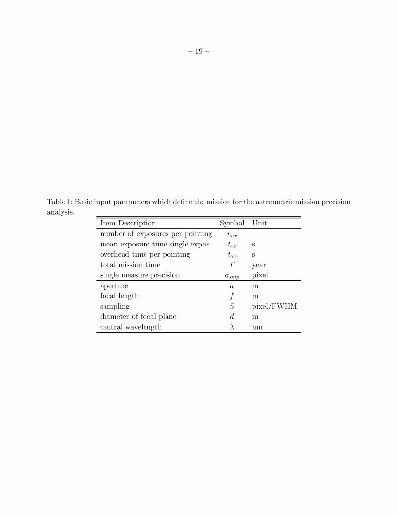
For the purpose at hand let the instrument and mission be defined by the set of basic

input parameters given in Table 1. In particular, the single measure precision, σsmp, is the

assumed error floor, a combination of random and systematic errors on the individual stellar

image centroiding level, and given as a fraction of a pixel. The σsmp will depend on the

astrometric quality of the hardware and thus be different from case to case as a function of

many technical details of the telescope, detector and operations. In the examples to follow

in section 5 realistic values are introduced for this free parameter. Astrometric quality is

explained in more detail in a design study of the USNO Robotic Astrometric Telescope

(Zacharias et al. 2006). Furthermore in the algorithm to follow a circular aperture and focal

plane is assumed, however any shape leads to the same conclusions.

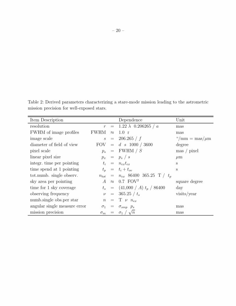
Table 2 summarizes the quantities derived from the set of basic parameters and also

shows the equations and units used. The goal is to arrive at the overall mission precision,

σm, for a single, stellar position coordinate of a star within the “sweet spot” of brightness.

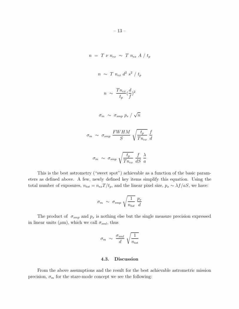
Using the algorithm of Table 2, quantities are then back substituted into the mission

precision, σm equation to allow only basic input parameters (Table 1). Dropping all numerical

scale factors (and some unit conversion factors) gives the following proportionality equations:

– 13 –

n = T ν nex ∼ T nex A / tp

n ∼ T nex d2 s2 / tp

n ∼Tnex

tp(d

f)2

σm ∼ σsmp ps /√

n

σm ∼ σsmp

FWHM

S

√

tpTnex

f

d

σm ∼ σsmp

√

tpTnex

f

dS

λ

a

This is the best astrometry (“sweet spot”) achievable as a function of the basic param-

eters as defined above. A few, newly defined key items simplify this equation. Using the

total number of exposures, ntot = nexT/tp, and the linear pixel size, px ∼ λf/aS, we have:

σm ∼ σsmp

√

1

ntot

px

d

The product of σsmp and px is nothing else but the single measure precision expressed

in linear units (µm), which we call σsml, thus

σm ∼σsml

d

√

1

ntot

4.3. Discussion

From the above assumptions and the result for the best achievable astrometric mission

precision, σm for the stare-mode concept we see the following:

– 14 –

1. The value for σm does NOT depend on the aperture of the telescope, nor the focal

length, nor the sampling. If we want to shift the “sweet spot” to a required magnitude,

this of course needs to be accomplished by a certain combination of aperture, exposure

time, throughput (bandwidth, quantum efficiency...) and mission lifetime. However,

the numeric value for the best astrometry remains unaffected by shifting it to a desired

magnitude, thus is independent of aperture, focal length, bandwidth and QE.

2. The σm does not depend on wavelength. Thus we are free to choose the spectral regime

we want the mission to operate in. The choice of a specific wavelength will require a

match between the focal length and pixel size with the desired sampling. This will not

affect the σm. However, manufacturability and alignment tolerances are better met for

a red than blue spectral bandpass. For a given, linear tolerance (fixed cost), the wave

front error as a fraction of the wavelength is smaller for red than for blue light which

buys an advantage in image quality.

3. The σm does not depend on the pixel size directly, however it does depend on the

product of pixel fraction error and pixel size, i.e. depends directly on the linear measure

precision in the focal plane. For very small pixels the limiting factor will be the physical

structures in the pixels, for very large pixels the limiting factor will be the pixel fraction

for the image centroiding. It is important to minimize σsml.

4. The driving factors toward smaller σm are a large number of single measurements and

a large focal plane. The large number of measures (with a constant mission life time)

implies many, short exposures with minimal overhead. This is somewhat contrary to

the basic mission concept, and particularly with a requirement to have many visits, as

for example for the science goals to detect many exo-planets. However, a very large

number of observations then heavily relies on the√

n law, which fails at some point

due to systematic errors.

5. The biggest and easiest impact on σm can be achieved by increasing the linear size of

the focal plane. Smaller astrometric errors can be obtained by spending more money

in the focal plane than for the aperture of the telescope optics. For sampling near

critical (≈ 2 pixel/FWHM) and for visible to near-infrared wavelengths the f-ratio of

the optical system will be slow (order f/30). This is an advantage for an optics design.

The focal length and the angular size of the field of view will only affect the number

of visits, not σm directly.

– 15 –

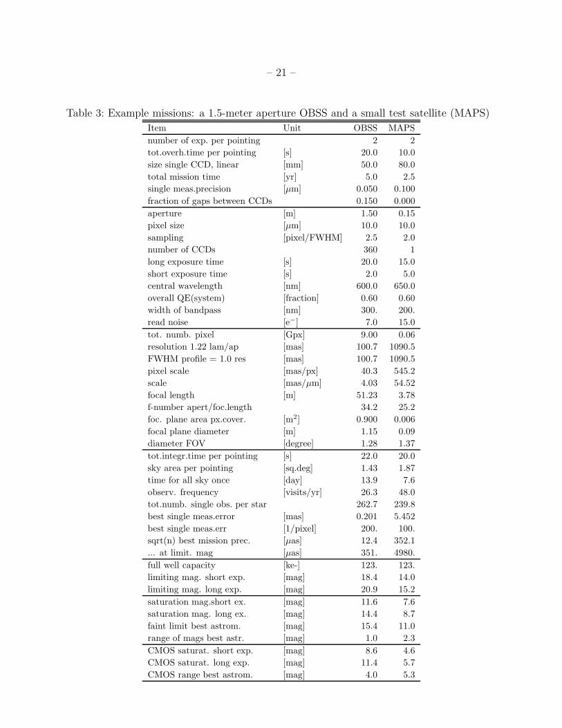
5. Examples

Table 3 gives numerical values for 2 example stare-mode missions, a large aperture

mission, like the current OBSS baseline, and a small, feasibility-study-type mission like

the Milli-arcsecond Pathfinder Survey (MAPS) satellite currently under study at USNO

(Dorland & Zacharias 2005; Dorland et al. 2005). MAPS will also be a technology demon-

stration mission, using a single, large-format CMOS or CMOS-hybrid detector. Even the

small MAPS mission would be capable of improving over Hipparcos by a factor of about

3 in positional precision and a factor of 100 in number of stars. The MAPS-like example

given in Table 3 gives about 250 µas mission precision for a single, well exposed star, while

the stated MAPS goal is to achieve at least 1 mas accuracy. For the MAPS mission the

required extragalactic targets would be near the limiting magnitude of the general all-sky

survey with unfavorable S/N ratio. However the flexibility of the stare-mode concept would

permit observation of the required number of relatively faint targets with more observations

and longer integration times.

The magnitudes at the bottom of Table 3 for the CMOS case assume that high precision

stellar image centroids can be obtained for stars up to 3.0 magnitudes brighter than the

saturation limit. No charge bleeding will be present and such bright stellar images can

be fitted using the unsaturated wings of the profile. This is a conservative estimate, good

astrometric results might be obtained for even brighter stars. The optical quality of the

observed point spread function on the 1% level of the peak intensity and below, straylight

and other factors will limit the astrometric quality of such centroids at some point if a stellar

image is vastly overexposed even if the detector does not bleed at all.

Expected results from the large OBSS-type mission are very much comparable to Gaia,

with the additional benefit of being able to reach fainter stars in a general all-sky survey

and going significantly deeper for targeted fields. For a comprehensive discussion of OBSS

capabilities and science goals see the NASA roadmap report by USNO (Johnston et al. 2004),

where also other issues of concern are mentioned together with suggested solutions. The

shutter issue, the required quality of the guiding, CPU power requirements, downlink rate

and several other issues of possible concern are not intractable problems.

Systematic errors will likely limit the performance of any astrometric mission. Compar-

ing the 2 FOV, large-angle measurement approach with the single FOV, differential mode,

both have to cope with imperfections of the optics and image centroiding issues. Imperfect

knowledge of field distortions, shifts of centroid positions as a function of magnitude and

color of the stars will affect both types of missions similarly, while performing accurate,

differential measures in the focal plane. A scanning mission might have some advantage be-

cause the signal for each observation is averaged over many pixels. The 2 FOV approach has

– 16 –

the disadvantage of absolute, large-angle measures with the basic angle stability problem, a

possible source of significant additional systematic errors.

6. Conclusions

For a Hipparcos-type mission the scanning operation concept was a good choice. With

no access to a sufficient number of extragalactic targets, large-angle measures (2 fields of

view separated by order of 90◦) are essential to obtain absolute parallaxes. Even today, if an

astrometric mission would be limited to 12th magnitude a Hipparcos-type concept would be

the way to go. For a mission capable of accessing extragalactic sources and being able to move

between fields fast as compared to the integration time, the stare-mode concept becomes a

viable alternative to the traditional 2-FOV scanning operation. Both conditions are met for

the stare-mode missions under consideration now (OBSS and MAPS). For these missions,

a 2-FOV scanning concept would still have the advantage of many individual observations,

which is important for some science goals like detecting extra-solar planets. The achievable

astrometric mission precisions are comparable between the scanning and stare-mode concept,

if the large square-root-n factor for a scanning mission can be believed for the mission

accuracy estimate. However, the stare-mode concept is a lower-risk approach with a high

single measure precision, a more conservative square-root-n factor and simpler engineering

requirements, thus lower costs. It has the advantage that no technology developments are

needed.

The major advantages of a stare-mode astrometric mission are the high degree of flexi-

bility, the higher astrometric precision in targeted areas, the ability to go significantly deeper

and the reduced complexity of the hardware with easier to achieve engineering requirements.

The stare-mode concept also potentially allows the use of radiation-hard CMOS detectors

which have an inherent large dynamic range (no blooming) thus also would allow low-risk

access to relatively bright stars, particularly in combination with short exposure times. Ex-

posure times in general are unrestricted in stare-mode operations, contrary to the scanning

mode of operation.

At this time, the stare-mode concept is not nearly as well developed as the scanning

satellite concept and detailed simulations will soon be performed to better understand the

exact requirements, capabilities and limitations. A particularly appealing aspect of a stare-

mode mission like OBSS is that it has the ability to be complementary or a replacement

mission depending on the observing schedule but using the same hardware. If Gaia performs

as predicted, a stare-mode mission can take the Gaia reference frame and concentrate on

deep, targeted fields. If Gaia does not perform as currently envisioned, the stare-mode

– 17 –

mission independently can fulfill most of Gaia’s science goals in a mainly general all-sky

survey. Furthermore, because the design is fundamentally different than Gaia, it offers

redundancy in case of problems in the Gaia implementation. A large enough stare-mode

mission could also substitute for many of the SIM targeted mission science. In order to get a

real proof-of-concept, a small, feasibility-study-type mission like MAPS is strongly suggested,

which could have a fast turnaround time and give valuable insight for the planning of a full-

scale mission.

The authors thank Ralph Gaume, Hugh Harris, Ken Johnston and Sean Urban for

valuable discussions and comments on the draft version of this paper. The referee is thanked

for many comments which lead to an improved paper.

REFERENCES

Benevides-Soares, P. & Teixeira, R., 1992, A&A, 253, 307

de Vegt, Chr., & Ebner, H., 1974, MNRAS, 167, 169

Dorland,B., Zacharias,N., Gaume,R., Johnston,K., Hennessy,G., Makarov,V., Rollins,C.,

2005, ”The Milli-Arcsecond Pathfinder Survey (MAPS) mission” AAS 207th meeting,

abstract 23.06, BAAS, 37, 1196

Dorland, B. & Zacharias, N. 2005, MAPS concept study, U.S. Naval Observatory, Washing-

ton, DC

Eichhorn, H., 1960, Astron. Nachr., 285, 233

ESA, 1997, The Hipparcos Catalogue, ESA SP-1200

Fuhrmann, U. 1979, PhD dissertation, University of Hamburg, Germany (Re-reduction of

the AGK2 with block adjustment methods)

Gaia 2000, Composition, Formation and Evolution of the Galaxy, ESA-SCI(2000)4, Con-

cept and Technoloy Study Report compiled by the Gaia Science Advisory Group

(eds. K.S.deBoer et al.)

Gaume, R. A. & Johnston, K. J. 2003, AMEX program team, AAS meeting 203, abstract

3.12

Googe, W. D., Eichhorn, H., & Lukac, C. F., 1970, MNRAS, 150, 35

– 18 –

Johnston, K. J. 2003, The FAME mission, Proc. SPIE 4854, 303, eds. J. C. Blades &

O. H. W. Siegmund

Johnston, K. J., Dorland, B. N., Gaume, R.A. et al. 2004, The Origins Billions Star Survey,

AAS meeting 205, abstr. 5.11

Johnston, K. J. et al. 2005, The Origins Billions Star Survey, NASA roadmap study,

U.S. Naval Observatory, Washington, DC

Johnston, K. J. et al. 2006, submitted to PASP

Lacroute, P. 1982, in Proc. The scientific aspects of the Hipparcos space astrometry mission,

ESA SP-177, p.3

van de Kamp, P. 1967, Principles of Astrometry, Freeman, San Francisco

Klemola, A. R., Hanson, R. B. & Jones, B. F. 1994, The Lick NPM program, Proc. Galactic

and Solar System Optical Astrometry, Eds. L.V. Morrison & G.F. Gilmore, Cambridge

Univ. Press, p.20

Makarov, V. V. & Milman, M. 2005, PASP, 117, 757

Makarov, V. V., Johnston, K.J., Zacharias, N. 2006, DDA meeting Halifax, Bull. AAS (in

press)

Platais, I., Kozhurina-Platais, V., Girard, T. M. et al. 1997, in Proc. ESA Sympos. Hipparcos-

Venice 97, ESA SP-402, p.153

Roser, S. 2000, in Working on the Fringe, ASP Conf.Series 194, p.68

Unwin, S. C., & Shao, M., 2000, Proc. SPIE, 4006, 754

Zacharias, M. I. & Zacharias, N. 2005, in Proc. Lowell astrometry meeting, ASP

Conf.Ser. 338, 184, Eds. P. K. Seidelman & A. Monet

Zacharias, N. 1988, Rigorous block-adjustment of the CPC2 Cape zone, Proc. IAU Sym-

pos. 133, ed. S.Debarbat, Kluwer, Dordrecht, p.201

Zacharias, N. 1992, A&A, 264, 296

Zacharias, N., Laux, U., Rakich, A., & Epps, H. 2006, in Proceedings of SPIE, Vol. 6267 (in

press)

This preprint was prepared with the AAS LATEX macros v5.2.

– 19 –

Table 1: Basic input parameters which define the mission for the astrometric mission precision

analysis.

Item Description Symbol Unit

number of exposures per pointing nex

mean exposure time single expos. tex s

overhead time per pointing tov s

total mission time T year

single measure precision σsmp pixel

aperture a m

focal length f m

sampling S pixel/FWHM

diameter of focal plane d m

central wavelength λ nm

– 20 –

Table 2: Derived parameters characterizing a stare-mode mission leading to the astrometric

mission precision for well-exposed stars.

Item Description Dependence Unit

resolution r = 1.22 λ 0.206265 / a mas

FWHM of image profiles FWHM ≈ 1.0 r mas

image scale s = 206.265 / f “/mm = mas/µm

diameter of field of view FOV = d s 1000 / 3600 degree

pixel scale ps = FWHM / S mas / pixel

linear pixel size px = ps / s µm

integr. time per pointing ti = nextex s

time spend at 1 pointing tp = ti + tov s

tot.numb. single observ. ntot = nex 86400 365.25 T / tpsky area per pointing A ≈ 0.7 FOV2 square degree

time for 1 sky coverage ts = (41,000 / A) tp / 86400 day

observing frequency ν = 365.25 / ts visits/year

numb.single obs.per star n = T ν nex

angular single measure error σ1 = σsmp ps mas

mission precision σm = σ1 /√

n mas

– 21 –

Table 3: Example missions: a 1.5-meter aperture OBSS and a small test satellite (MAPS)

Item Unit OBSS MAPS

number of exp. per pointing 2 2

tot.overh.time per pointing [s] 20.0 10.0

size single CCD, linear [mm] 50.0 80.0

total mission time [yr] 5.0 2.5

single meas.precision [µm] 0.050 0.100

fraction of gaps between CCDs 0.150 0.000

aperture [m] 1.50 0.15

pixel size [µm] 10.0 10.0

sampling [pixel/FWHM] 2.5 2.0

number of CCDs 360 1

long exposure time [s] 20.0 15.0

short exposure time [s] 2.0 5.0

central wavelength [nm] 600.0 650.0

overall QE(system) [fraction] 0.60 0.60

width of bandpass [nm] 300. 200.

read noise [e−] 7.0 15.0

tot. numb. pixel [Gpx] 9.00 0.06

resolution 1.22 lam/ap [mas] 100.7 1090.5

FWHM profile = 1.0 res [mas] 100.7 1090.5

pixel scale [mas/px] 40.3 545.2

scale [mas/µm] 4.03 54.52

focal length [m] 51.23 3.78

f-number apert/foc.length 34.2 25.2

foc. plane area px.cover. [m2] 0.900 0.006

focal plane diameter [m] 1.15 0.09

diameter FOV [degree] 1.28 1.37

tot.integr.time per pointing [s] 22.0 20.0

sky area per pointing [sq.deg] 1.43 1.87

time for all sky once [day] 13.9 7.6

observ. frequency [visits/yr] 26.3 48.0

tot.numb. single obs. per star 262.7 239.8

best single meas.error [mas] 0.201 5.452

best single meas.err [1/pixel] 200. 100.

sqrt(n) best mission prec. [µas] 12.4 352.1

... at limit. mag [µas] 351. 4980.

full well capacity [ke-] 123. 123.

limiting mag. short exp. [mag] 18.4 14.0

limiting mag. long exp. [mag] 20.9 15.2

saturation mag.short ex. [mag] 11.6 7.6

saturation mag. long ex. [mag] 14.4 8.7

faint limit best astrom. [mag] 15.4 11.0

range of mags best astr. [mag] 1.0 2.3

CMOS saturat. short exp. [mag] 8.6 4.6

CMOS saturat. long exp. [mag] 11.4 5.7

CMOS range best astrom. [mag] 4.0 5.3