The Common Patterns of Nature Steven A. Frank * June 18, 2009 Please cite as follows: Frank, S. A. 2009. The common patterns of nature. Journal of Evolutionary Biology XX:XXX–XXX. [Check link below for final volume and page numbers.] The published, definitive version of this article is freely available at: http://dx.doi.org/10.1111/j.1420-9101.2009.01775.x * Department of Ecology and Evolutionary Biology, University of California, Irvine, CA 92697– 2525, USA and Santa Fe Institute, 1399 Hyde Park Road, Santa Fe, NM 87501, USA, email: [email protected] 1 arXiv:0906.3507v1 [q-bio.QM] 18 Jun 2009

Welcome message from author
This document is posted to help you gain knowledge. Please leave a comment to let me know what you think about it! Share it to your friends and learn new things together.
Transcript

The Common Patterns of Nature
Steven A. Frank∗
June 18, 2009
Please cite as follows: Frank, S. A. 2009. The common patterns of nature.
Journal of Evolutionary Biology XX:XXX–XXX. [Check link below for final volume
and page numbers.]
The published, definitive version of this article is freely available at:
http://dx.doi.org/10.1111/j.1420-9101.2009.01775.x
∗Department of Ecology and Evolutionary Biology, University of California, Irvine, CA 92697–
2525, USA and Santa Fe Institute, 1399 Hyde Park Road, Santa Fe, NM 87501, USA, email:
1
arX
iv:0
906.
3507
v1 [
q-bi
o.Q
M]
18
Jun
2009
Abstract
We typically observe large-scale outcomes that arise from the interactions of many
hidden, small-scale processes. Examples include age of disease onset, rates of
amino acid substitutions, and composition of ecological communities. The macro-
scopic patterns in each problem often vary around a characteristic shape that can
be generated by neutral processes. A neutral generative model assumes that each
microscopic process follows unbiased or random stochastic fluctuations: random
connections of network nodes; amino acid substitutions with no effect on fitness;
species that arise or disappear from communities randomly. These neutral gener-
ative models often match common patterns of nature. In this paper, I present the
theoretical background by which we can understand why these neutral generative
models are so successful. I show where the classic patterns come from, such as the
Poisson pattern, the normal or Gaussian pattern, and many others. Each classic
pattern was often discovered by a simple neutral generative model. The neutral
patterns share a special characteristic: they describe the patterns of nature that
follow from simple constraints on information. For example, any aggregation of
processes that preserves information only about the mean and variance attracts
to the Gaussian pattern; any aggregation that preserves information only about
the mean attracts to the exponential pattern; any aggregation that preserves in-
formation only about the geometric mean attracts to the power law pattern. I
present a simple and consistent informational framework of the common patterns
of nature based on the method of maximum entropy. This framework shows that
each neutral generative model is a special case that helps to discover a particu-
lar set of informational constraints; those informational constraints define a much
wider domain of non-neutral generative processes that attract to the same neutral
pattern.
2
In fact, all epistemologic value of the theory of probability is based
on this: that large-scale random phenomena in their collective action
create strict, nonrandom regularity (Gnedenko & Kolmogorov, 1968,
p. 1).
I know of scarcely anything so apt to impress the imagination as the
wonderful form of cosmic order expressed by the “law of frequency of
error” [the normal or Gaussian distribution]. Whenever a large sample
of chaotic elements is taken in hand and marshaled in the order of
their magnitude, this unexpected and most beautiful form of regularity
proves to have been latent all along. The law . . . reigns with serenity
and complete self-effacement amidst the wildest confusion. The larger
the mob and the greater the apparent anarchy, the more perfect is its
sway. It is the supreme law of unreason (Galton, 1889, p. 166).
We cannot understand what is happening until we learn to think
of probability distributions in terms of their demonstrable information
content . . . (Jaynes, 2003, p. 198).
Introduction
Most patterns in biology arise from aggregation of many small processes. Vari-
ations in the dynamics of complex neural and biochemical networks depend on
numerous fluctuations in connectivity and flow through small-scale subcompo-
nents of the network. Variations in cancer onset arise from variable failures in the
many individual checks and balances on DNA repair, cell cycle control, and tissue
homeostasis. Variations in the ecological distribution of species follow the myr-
iad local differences in the birth and death rates of species and in the small-scale
interactions between particular species.
In all such complex systems, we wish to understand how large-scale pattern
arises from the aggregation of small-scale processes. A single dominant principle
sets the major axis from which all explanation of aggregation and scale must be
developed. This dominant principle is the limiting distribution.
3
The best known of the limiting distributions, the Gaussian (normal) distribu-
tion, follows from the central limit theorem. If an outcome, such as height, weight,
or yield, arises from the summing up of many small-scale processes, then the dis-
tribution typically approaches the Gaussian curve in the limit of aggregation over
many processes.
The individual, small-scale fluctuations caused by each contributing process
rarely follow the Gaussian curve. But, with aggregation of many partly uncorre-
lated fluctuations, each small in scale relative to the aggregate, the sum of the fluc-
tuations smooths into the Gaussian curve—the limiting distribution in this case.
One might say that the numerous small fluctuations tend to cancel out, revealing
the particular form of regularity or information that characterizes aggregation and
scale for the process under study.
The central limit theorem is widely known, and the Gaussian distribution is
widely recognized as an aggregate pattern. This limiting distribution is so im-
portant that one could hardly begin to understand patterns of nature without an
instinctive recognition of the relation between aggregation and the Gaussian curve.
In this paper, I discuss biological patterns within a broader framework of lim-
iting distributions. I emphasize that the common patterns of nature arise from
distinctive limiting distributions. In each case, one must understand the distinctive
limiting distribution in order to analyze pattern and process.
In regard to the different limiting distributions that characterize patterns of
nature, aggregation and scale have at least three important consequences. First,
a departure from the expected limiting distribution suggests an interesting pro-
cess that perturbs the typical regularity of aggregation. Such departures from
expectation can only be recognized and understood if one has a clear grasp of the
characteristic limiting distribution for the particular problem.
Second, one must distinguish clearly between two distinct meanings of “neu-
trality.” For example, if we count the number of events of a purely random, or
“neutral,” process, we observe a Poisson pattern. However, the Poisson may also
arise as a limiting distribution by aggregation of small-scale, nonrandom processes.
So we must distinguish between two alternative causes of neutral pattern: the gen-
eration of pattern by neutral processes, or the generation of pattern by aggregation
4

of non-neutral processes in which the non-neutral fluctuations tend to cancel in the
aggregate. This distinction cuts to the heart of how we may test neutral theories
in ecology and evolution.
Third, a powerfully attracting limiting distribution may be relatively insen-
sitive to perturbations. Insensitivity arises because, to be attracting over broad
variations in the aggregated processes, the limiting distribution must not change
too much in response to perturbations. Insensitivity to perturbation is a reasonable
definition of robustness. Thus, robust patterns may often coincide with limiting
distributions.
In general, inference in biology depends critically on understanding the nature
of limiting distributions. If a pattern can only be generated by a very particular
hypothesized process, then observing the pattern strongly suggests that the pattern
was created by the hypothesized generative process. By contrast, if the same
pattern arises as a limiting distribution from a variety of underlying processes,
then a match between theory and pattern only restricts the underlying generative
processes to the broad set that attracts to the limiting pattern. Inference must
always be discussed in relation to the breadth of processes attracted to a particular
pattern. Because many patterns in nature arise from limiting distributions, such
distributions form the core of inference with regard to the relations between pattern
and process.
I recently took up study of the problems outlined in this introduction. In my
studies, I found it useful to separate the basic facts of probability theory that set
the background from my particular ideas about biological robustness, the neutral
theories in ecology and evolution, and the causes of patterns such as the age of
cancer onset and the age of death. The basic facts of probability are relatively
uncontroversial, whereas my own interpretations of particular biological patterns
remain open to revision and to the challenge of empirical tests.
In this paper, I focus on the basic facts of probability theory to set the back-
ground for future work. Thus, this paper serves primarily as a tutorial to aspects
of probability framed in the context of several recent conceptual advances from
the mathematical and physical sciences. In particular, I use Jaynes’ maximum
entropy approach to unify the relations between aggregation and pattern (Jaynes,
5

2003). Information plays the key role. In each problem, ultimate pattern arises
from the particular information preserved in the face of the combined fluctuations
in aggregates that decay all non-preserved aspects of pattern toward maximum
entropy or maximum randomness. My novel contribution is to apply this frame-
work of entropy and information in a very simple and consistent way across the
full range of common patterns in nature.
Overview
The general issues of aggregation and limiting distributions are widely known
throughout the sciences, particularly in physics. These concepts form the basis for
much of statistical mechanics and thermodynamics. Yet, in spite of all of this work,
the majority of research in biology remains outside the scope of these fundamental
and well understood principles. Indeed, much of the biological literature continues
as if the principles of aggregation and scale hardly existed, in spite of a few well
argued publications that appear within each particular subject.
Three reasons may explain the disconnect between, on the one hand, the prin-
ciples of aggregation and scale, and, on the other hand, the way in which different
subfields of biology often deal with the relations between pattern and process.
First, biologists are often unaware of the general quantitative principles, and lack
experience with and exposure to other quantitative fields of science. Second, each
subfield within biology tends to struggle with the fundamental issues independently
of other subfields. Little sharing occurs of the lessons slowly learned within distinct
subfields. Third, in spite of much mathematical work on aggregation and limiting
distributions, many fundamental issues remain unresolved or poorly connected to
commonly observed phenomena. For example, power law distributions arise in
economics and in nearly every facet of nature. Almost all theories to explain the
observed power law patterns emphasize either particular models of process, which
have limited scope, or overly complex theories of entropy and aggregation, which
seem too specialized to form a general explanation.
I begin with two distinct summaries of the basic quantitative principles. In
the first summary, I discuss in an intuitive way some common distributions that
6
describe patterns of nature: the exponential, Poisson, and gamma distributions.
These distributions often associate with the concepts of random or neutral pro-
cesses, setting default expectations about pattern. I emphasize the reason these
patterns arise so often: combinations of many small-scale processes tend to yield,
at a higher, aggregate scale, these common distributions. We call the observed pat-
terns from such aggregation the limiting distributions, because these distributions
arise in the limit of aggregation, at a larger scale, over many partially uncorre-
lated processes at smaller scales. The small-scale fluctuations tend to cancel out
at the larger scale, yielding observed patterns that appear random, or neutral,
even though the pattern is created by aggregation of nonrandom processes.
In my second summary of the basic quantitative principles, I give a slightly
more technical description. In particular, I discuss what “random” means, and why
aggregation of nonrandom processes leads in the limit to the random or neutral
patterns at larger scales.
The following sections discuss aggregation more explicitly. I emphasize how
processes interact to form aggregate pattern, and how widespread such aggregation
must be. Certain general patterns arise as the most fundamental outcomes of
aggregation, of which the Gaussian distribution and the central limit theorem are
special cases.
Finally, I conclude that the most important consequences of aggregation are
simple yet essential to understand: certain patterns dominate for particular fields
of study; those patterns set a default against which deviations must be understood;
and the key to inference turns on understanding the separation between those
small-scale processes that tend to attract in the aggregate to the default pattern
and those small-scale processes that do not aggregate to the default pattern.
Common distributions
This section provides brief, intuitive descriptions of a few important patterns ex-
pressed as probability distributions. These descriptions set the stage for the more
comprehensive presentation in the following section. Numerous books provide
introductions to common probability distributions and relevant aspects of proba-
7

bility theory (e.g., Feller, 1968, 1971; N. L. Johnson et al ., 1994, 2005; Kleiber &
Kotz, 2003).
Poisson
One often counts the number of times an event occurs per unit area or per unit
time. When the numbers per unit of measurement are small, the observations often
follow the Poisson distribution. The Poisson defines the neutral or random expec-
tation for pattern, because the Poisson pattern arises when events are scattered at
random over a grid of spatial or temporal units.
A standard test for departure from randomness compares observations against
the random expectations that arise from the Poisson distribution. A common
interpretation from this test is that a match between observations and the Poisson
expectation implies that the pattern was generated by a neutral or random process.
However, to evaluate how much information one obtains from such a match, one
must know how often aggregations of nonrandom processes may generate the same
random pattern.
Various theorems of probability tell us when particular combinations of under-
lying, smaller scale processes lead to a Poisson pattern at the larger, aggregate
scale. Those theorems, which I discuss in a later section, define the “law of small
numbers.” From those theorems, we get a sense of the basin of attraction to the
Poisson as a limiting distribution: in other words, we learn about the separation
between those aggregations of small-scale processes that combine to attract toward
the Poisson pattern and those aggregations that do not.
Here is a rough, intuitive way to think about the basin of attraction toward a
random, limiting distribution (Jaynes, 2003). Think of each small-scale process as
contributing a deviation from random in the aggregate. If many nonrandom and
partially uncorrelated small-scale deviations aggregate to form an overall pattern,
then the individual nonrandom deviations will often cancel in the aggregate and
attract to the limiting random distribution. Such smoothing of small-scale devia-
tions in the aggregate pattern must be rather common, explaining why a random
pattern with strict regularity, such as the Poisson, is so widely observed.
8

Many aggregate patterns will, of course, deviate from the random limiting
distribution. To understand such deviations, we must consider them in relation
to the basin of attraction for random pattern. In general, the basins of attraction
of random patterns form the foundation by which we must interpret observations
of nature. In this regard, the major limiting distributions are the cornerstone of
natural history.
Exponential and gamma
The waiting time for the first occurrence of some particular event often follows an
exponential distribution. The exponential has three properties that associate it
with a neutral or random pattern.
First, the waiting time until the first occurrence of a Poisson process has an
exponential distribution: the exponential is the time characterization of how long
one waits for random events, and the Poisson is the count characterization of the
number of random events that occur in a fixed time (or space) interval.
Second, the exponential distribution has the memoryless property. Suppose
the waiting time for the first occurrence of an event follows the exponential distri-
bution. If, starting at time t = 0, the event does not occur during the interval up
to time t = T , then the waiting time for the first occurrence starting from time T
is the same as it was when we began to measure from time zero. In other words,
the process has no memory of how long it has been waiting; occurrences happen
at random irrespective of history.
Third, the exponential is in many cases the limiting distribution for aggregation
of smaller-scale waiting time processes (see below). For example, time to failure
patterns often follow the exponential, because the failure of a machine or aggregate
biological structure often depends on the time to failure of any essential component.
Each component may have a time to failure that differs from exponential, but in the
aggregate, the waiting time for the overall failure of the machine often converges
to the exponential.
The gamma distribution arises in many ways, a characteristic of limiting dis-
tributions. For example, if the waiting time until the first occurrence of a random
9
process follows an exponential, and occurrences happen independently of each
other, then the waiting time for the nth occurrence follows the gamma pattern.
The exponential is a limiting distribution with a broad basin of attraction. Thus,
the gamma is also a limiting distribution that attracts many aggregate patterns.
For example, if an aggregate structure fails only after multiple subcomponents fail,
then the time to failure may in the limit attract to a gamma pattern. In a later
section, I will discuss a more general way in which to view the gamma distribution
with respect to randomness and limiting distributions.
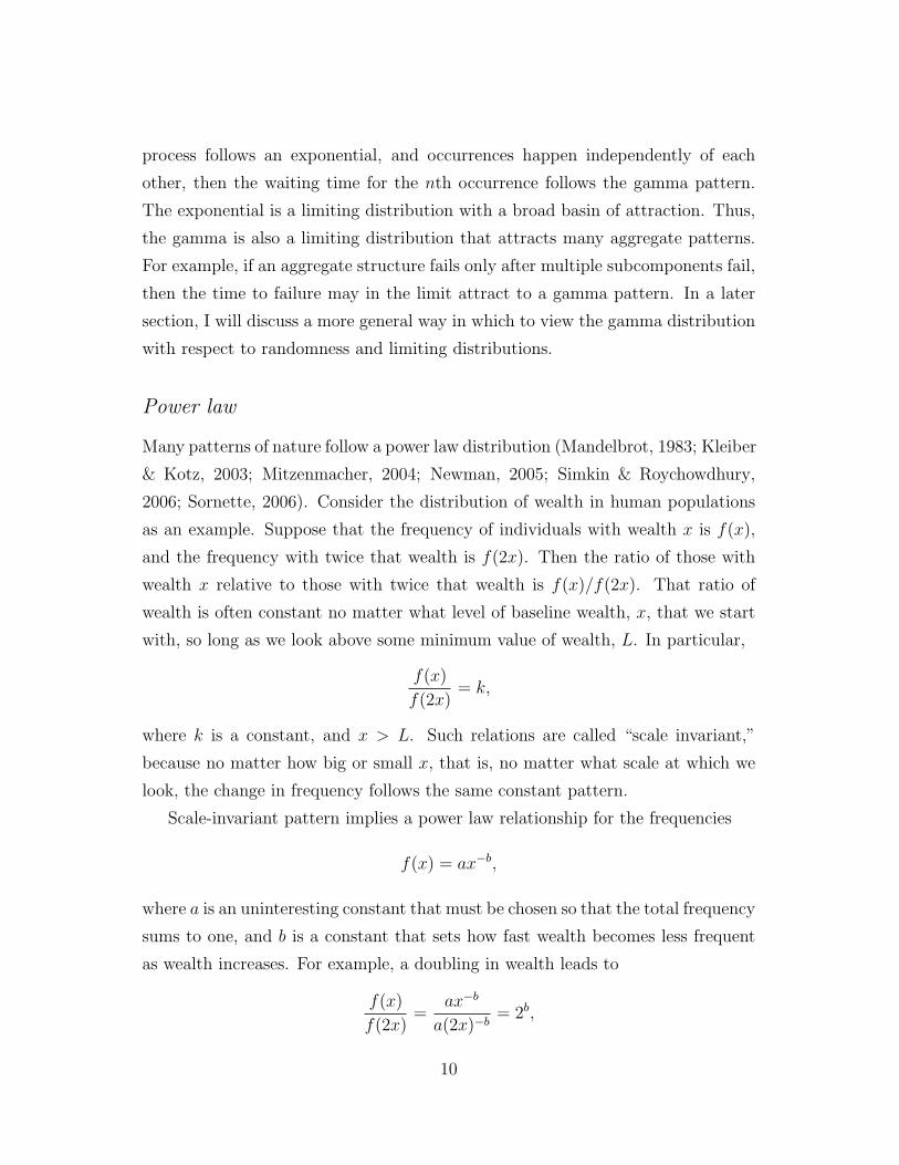
Power law
Many patterns of nature follow a power law distribution (Mandelbrot, 1983; Kleiber
& Kotz, 2003; Mitzenmacher, 2004; Newman, 2005; Simkin & Roychowdhury,
2006; Sornette, 2006). Consider the distribution of wealth in human populations
as an example. Suppose that the frequency of individuals with wealth x is f(x),
and the frequency with twice that wealth is f(2x). Then the ratio of those with
wealth x relative to those with twice that wealth is f(x)/f(2x). That ratio of
wealth is often constant no matter what level of baseline wealth, x, that we start
with, so long as we look above some minimum value of wealth, L. In particular,
f(x)
f(2x)= k,
where k is a constant, and x > L. Such relations are called “scale invariant,”
because no matter how big or small x, that is, no matter what scale at which we
look, the change in frequency follows the same constant pattern.
Scale-invariant pattern implies a power law relationship for the frequencies
f(x) = ax−b,
where a is an uninteresting constant that must be chosen so that the total frequency
sums to one, and b is a constant that sets how fast wealth becomes less frequent
as wealth increases. For example, a doubling in wealth leads to
f(x)
f(2x)=
ax−b
a(2x)−b= 2b,
10
which shows that the ratio of the frequency of people with wealth x relative to
those with wealth 2x does not depend on the initial wealth, x, that is, it does not
depend on the scale at which we look.
Scale invariance, expressed by power laws, describes a very wide range of nat-
ural patterns. To give just a short listing, Sornette (2006) mentions that the fol-
lowing phenomena follow power law distributions: the magnitudes of earthquakes,
hurricanes, volcanic eruptions, and floods; the sizes of meteorites; and losses caused
by business interruptions from accidents. Other studies have documented power
laws in stock market fluctuations, sizes of computer files, and word frequency in
languages (Mitzenmacher, 2004; Newman, 2005; Simkin & Roychowdhury, 2006).
In biology, power laws have been particularly important in analyzing connectiv-
ity patterns in metabolic networks (Barabasi & Albert, 1999; Ravasz et al ., 2002)
and in the number of species observed per unit area in ecology (Garcia Martin &
Goldenfeld, 2006).
Many models have been developed to explain why power laws arise. Here is a
simple example from Simon (1955) to explain the power law distribution of word
frequency in languages (see Simkin & Roychowdhury, 2006). Suppose we start
with a collection of N words. We then add another word. With probability p, the
word is new. With probability 1−p, the word matches one already in our collection;
the particular match to an existing word occurs with probability proportional to
the relative frequencies of existing words. In the long run, the frequency of words
that occurs x times is proportional to x−[1+1/(1−p)]. We can think of this process
as preferential attachment, or an example in which the rich get richer.
Simon’s model sets out a simple process that generates a power law and fits
the data. But could other simple processes generate the same pattern? We can
express this question in an alternative way, following the theme of this paper:
What is the basin of attraction for processes that converge onto the same pattern?
The following sections take up this question and, more generally, how we may think
about the relationship between generative models of process and the commonly
observed patterns that result.
11

Random or neutral distributions
Much of biological research is reverse engineering. We observe a pattern or design,
and we try to infer the underlying process that generated what we see. The ob-
served patterns can often be described as probability distributions: the frequencies
of genotypes; the numbers of nucleotide substitutions per site over some stretch of
DNA; the different output response strengths or movement directions given some
input; or the numbers of species per unit area.
The same small set of probability distributions describe the great majority
of observed patterns: the binomial, Poisson, Gaussian, exponential, power law,
gamma, and a few other common distributions. These distributions reveal the
contours of nature. We must understand why these distributions are so common
and what they tell us, because our goal is to use these observed patterns to reverse
engineer the underlying processes that created those patterns. What information
do these distributions contain?
Maximum entropy
The key probability distributions often arise as the most random pattern consistent
the information expressed by a few constraints (Jaynes, 2003). In this section, I in-
troduce the concept of maximum entropy, where entropy measures randomness. In
the following sections, I derive common distributions to show how they arise from
maximum entropy (randomness) subject to constraints such as information about
the mean, variance, or geometric mean. My mathematical presentation through-
out is informal and meant to convey basic concepts. Those readers interested in
the mathematics should follow the references to the original literature.
The probability distributions follow from Shannon’s measure of information
(Shannon & Weaver, 1949). I first define this measure of information. I then
discuss an intuitive way of thinking about the measure and its relation to entropy.
Consider a probability distribution function (pdf) defined as p(y|θ). Here, p
is the probability of some measurement y given a set of parameters, θ. Let the
abbreviation py stand for p(y|θ). Then Shannon information is defined as
H = −∑
py log(py),
12

where the sum is taken over all possible values of y, and the log is taken as the
natural logarithm.
The value − log(py) = log(1/py) rises as the probability py of observing a
particular value of y becomes smaller. In other words, − log(py) measures the
surprise in observing a particular value of y, because rare events are more surprising
(Tribus, 1961). Greater surprise provides more information: if we are surprised by
an observation, we learn a lot; if we are not surprised, we had already predicted
the outcome to be likely, and we gain little information. With this interpretation,
Shannon information, H, is simply an average measure of surprise over all possible
values of y.
We may interpret the maximum of H as the least predictable and most random
distribution within the constraints of any particular problem. In physics, random-
ness is usually expressed in terms of entropy, or disorder, and is measured by the
same expression as Shannon information. Thus, the technique of maximizing H
to obtain the most random distribution subject to the constraints of a particular
problem is usually referred to as the method of maximum entropy (Jaynes, 2003).
Why should observed probability distributions tend toward those with maxi-
mum entropy? Because observed patterns typically arise by aggregation of many
small scale processes. Any directionality or nonrandomness caused by each small
scale process tends, on average, to be canceled in the aggregate: one fluctuation
pushes in one direction, another fluctuation pushes in a different direction, and so
on. Of course, not all observations are completely random. The key is that each
problem typically has a few constraints that set the pattern in the aggregate, and
all other fluctuations cancel as the nonconstrained aspects tend to the greatest
entropy or randomness. In terms of information, the final pattern reflects only the
information content of the system expressed by the constraints on randomness;
all else dissipates to maximum entropy as the pattern converges to its limiting
distribution defined by its informational constraints (Van Campenhout & Cover,
1981).
13
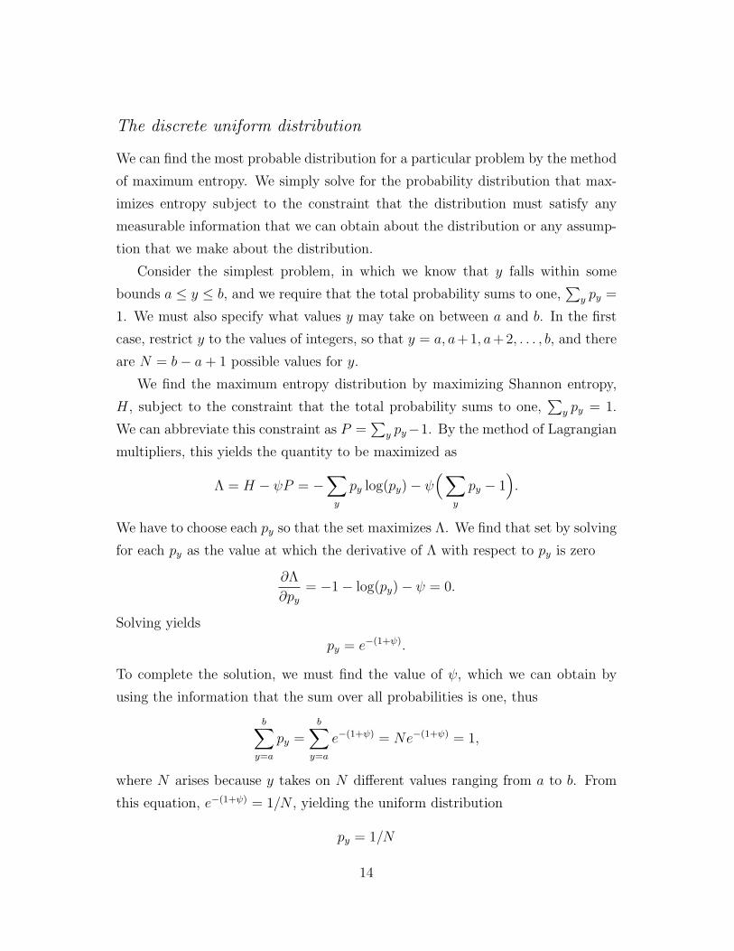
The discrete uniform distribution
We can find the most probable distribution for a particular problem by the method
of maximum entropy. We simply solve for the probability distribution that max-
imizes entropy subject to the constraint that the distribution must satisfy any
measurable information that we can obtain about the distribution or any assump-
tion that we make about the distribution.
Consider the simplest problem, in which we know that y falls within some
bounds a ≤ y ≤ b, and we require that the total probability sums to one,∑
y py =
1. We must also specify what values y may take on between a and b. In the first
case, restrict y to the values of integers, so that y = a, a+ 1, a+ 2, . . . , b, and there
are N = b− a+ 1 possible values for y.
We find the maximum entropy distribution by maximizing Shannon entropy,
H, subject to the constraint that the total probability sums to one,∑
y py = 1.
We can abbreviate this constraint as P =∑
y py−1. By the method of Lagrangian
multipliers, this yields the quantity to be maximized as
Λ = H − ψP = −∑y
py log(py)− ψ(∑
y
py − 1).
We have to choose each py so that the set maximizes Λ. We find that set by solving
for each py as the value at which the derivative of Λ with respect to py is zero
∂Λ
∂py= −1− log(py)− ψ = 0.
Solving yields
py = e−(1+ψ).
To complete the solution, we must find the value of ψ, which we can obtain by
using the information that the sum over all probabilities is one, thus
b∑y=a
py =b∑
y=a
e−(1+ψ) = Ne−(1+ψ) = 1,
where N arises because y takes on N different values ranging from a to b. From
this equation, e−(1+ψ) = 1/N , yielding the uniform distribution
py = 1/N
14
for y = a, . . . , b. This result simply says that if we do not know anything except
the possible values of our observations and the fact that the total probability is
one, then we should consider all possible outcomes equally (uniformly) probable.
The uniform distribution is sometimes discussed as the expression of ignorance or
lack of information.
In observations of nature, we usually can obtain some additional information
from measurement or from knowledge about the structure of the problem. Thus,
the uniform distribution does not describe well many patterns of nature, but rather
arises most often as an expression of prior ignorance before we obtain information.
The continuous uniform distribution
The previous section derived the uniform distribution in which the observations y
take on integer values a, a + 1, a + 2, . . . , b. In this section, I show the steps and
notation for the continuous uniform case. See Jaynes (2003) for technical issues
that may arise when analyzing maximum entropy for continuous variables.
Everything is the same as the previous section, except that y can take on any
continuous value between a and b. We can move from the discrete case to the
continuous case by writing the possible values of y as a, a+ dy, a+ 2dy, . . . , b. In
the discrete case above, dy = 1. In the continuous case, we let dy → 0, that is,
we let dy become arbitrarily small. Then the number of steps between a and b is
(b− a)/dy.
The analysis is exactly as above, but each increment must be weighted by dy,
and instead of writingb∑
y=a
pydy = 1
we write ∫ b
a
pydy = 1
to express integration of small units, dy, rather than summation of discrete units.
Then, repeating the key equations from above in the continuous notation, we have
the basic expression of the value to be maximized as
Λ = H − ψP = −∫y
py log(py)dy − ψ(∫
y
pydy − 1
).
15

From the prior section, we know ∂Λ/∂py = 0 leads to py = e−(1+ψ), thus∫ b
a
pydy =
∫ b
a
e−(1+ψ)dy = (b− a)e−(1+ψ) = 1,
where b− a arises because∫ ba
dy = b− a, thus e−(1+ψ) = 1/(b− a), and
py =1
b− a,
which is the uniform distribution over the continuous interval between a and b.
The binomial distribution
The binomial distribution describes the outcome of a series of i = 1, 2, . . . , N
observations or trials. Each observation can take on one of two values, xi = 0 or
xi = 1, for the ith observation. For convenience, we refer to an observation of one
as a success, and an observation of zero as a failure. We assume each observation
is independent of the others, and the probability of a success on any trial is ai,
where ai may vary from trial to trial. The total number of successes over N trials
is y =∑xi.
Suppose this is all the information that we have. We know that our random
variable, y, can take on a series of integer values, y = 0, 1, . . . , N , because we
may have between zero and N total successes in N trials. Define the probability
distribution as py, the probability that we observe y successes in N trials. We know
that the probabilities sum to one. Given only that information, it may seem, at
first glance, that the maximum entropy distribution would be uniform over the
possible outcomes for y. However, the structure of the problem provides more
information, which we must incorporate.
How many different ways can we can obtain y = 0 successes in N trials? Just
one: a series of failures on every trial. How many different ways can we obtain
y = 1 success? There are N different ways: a success on the first trial and failures
on the others; a success on the second trial, and failures on the others; and so on.
The uniform solution by maximum entropy tells us that each different combi-
nation is equally likely. Because each value of y maps to a different number of
combinations, we must make a correction for the fact that measurements on y are
16
distinct from measurements on the equally likely combinations. In particular, we
must formulate a measure, my, that accounts for how the uniformly distributed
basis of combinations translates into variable values of the number of successes, y.
Put another way, y is invariant to changes in the order of outcomes given a fixed
number of successes. That invariance captures a lack of information that must be
included in our analysis.
This use of a transform to capture the nature of measurement in a particular
problem recurs in analyses of entropy. The proper analysis of entropy must be
made with respect to the underlying measure. We replace the Shannon entropy
with the more general expression
S = −∑
py log
[pymy
], (1)
a measure of relative entropy that is related to the Kullback-Leibler divergence
(Kullback, 1959). When my is a constant, expressing a uniform transformation,
then we recover the standard expression for Shannon entropy.
In the binomial sampling problem, the number of combinations for each value
of y is
my =
(N
y
)=
N !
y!(N − y)!. (2)
Suppose that we also know the expected number of successes in a series of
N trials, given as 〈y〉 =∑ypy, where I use the physicists’ convention of angle
brackets for the expectation of the quantity inside. Earlier, I defined ai as the
probability of success in the ith trial. Note that the average probability of success
per trial is 〈y〉/N = 〈a〉. For convenience, let α = 〈a〉, thus the expected number
of successes is 〈y〉 = Nα.
What is the maximum entropy distribution given all of the information that
we have, including the expected number of successes? We proceed by maximizing
S subject to the constraint that all the probabilities must add to one and subject
to the constraint, C1 =∑ypy −Nα, that the mean number of successes must be
〈y〉 = Nα. The quantity to maximize is
Λ = S − ψP − λ1C1
= −∑
py log
[pymy
]− ψ
(∑py − 1
)− λ1
(∑ypy −Nα
).
17
Differentiating with respect to py and setting to zero yields
py = k
(N
y
)e−λ1y, (3)
where k = e−(1+ψ), in which k and λ1 are two constants that must be chosen to
satisfy the two constraints∑py = 1 and
∑ypy = Nα. The constants k = (1−α)N
and e−λ1 = α/(1− α) satisfy the two constraints (Sivia & Skilling, 2006, pp. 115–
120) and yield the binomial distribution
py =
(N
y
)αy(1− α)N−y.
Here is the important conclusion. If all of the information available in mea-
surement reduces to knowledge that we are observing the outcome of a series of
binary trials and to knowledge of the average number of successes in N trials, then
the observations will follow the binomial distribution.
In the classic sampling theory approach to deriving distributions, one generates
a binomial distribution by a series of independent, identical binary trials in which
the probability of success per trial does not vary between trials. That generative
neutral model does create a binomial process—it is a sufficient condition.
However, many distinct processes may also converge to the binomial pattern.
One only requires information about the trial-based sampling structure and about
the expected number of successes over all trials. The probability of success may
vary between trials (Yu, 2008).
Distinct aggregations of small scale processes may smooth to reveal only those
two aspects of information—sampling structure and average number of successes—
with other measurable forms of information canceling in the aggregate. Thus,
the truly fundamental nature of the binomial pattern arises not from the neutral
generative model of identical, independent binary trials, but from the measurable
information in observations. I discuss some additional processes that converge to
the binomial in a later section on limiting distributions.
The Poisson distribution
One often observes a Poisson distribution when counting the number of observa-
tions per unit time or per unit area. The Poisson occurs so often because it arises
18
from the “law of small numbers,” in which aggregation of various processes con-
verges to the Poisson when the number of counts per unit is small. Here, I derive
the Poisson as a maximum entropy distribution subject to a constraint on the
sampling process and a constraint on the mean number of counts per unit (Sivia
& Skilling, 2006, pp. 121).
Suppose the unit of measure, such as time or space, is divided into a great
number, N , of very small intervals. For whatever item or event we are counting,
each interval contains a count of either zero or one that is independent of the counts
in other intervals. This subdivision leads to a binomial process. The measure for
the number of different ways a total count of y = 0, 1, . . . , N can arise in the N
subdivisions is given by my of Eq. (2). With large N , we can express this measure
by using Stirling’s approximation
N ! ≈√
2πN(N/e)N ,
where e is the base for the natural logarithm. Using this approximation for large
N , we obtain
my =
(N
y
)=
N !
y!(N − y)!=Ny
y!.
Entropy maximization yields Eq. (3), in which we can use the large N approxima-
tion for my to yield
py = kxy
y!,
in which x = Ne−λ1 . From this equation, the constraint∑py = 1 leads to the
identity∑
y xy/y! = ex, which implies k = e−x. The constraint
∑ypy = 〈y〉 = µ
leads to the identity∑
y yxy/y! = xex, which implies x = µ. These substitutions
for k and x yield the Poisson distribution
py = µye−µ
y!.
The general solution
All maximum entropy problems have the same form. We first evaluate our in-
formation about the scale of observations and the sampling scheme. We use this
information to determine the measure my in the general expression for relative
19
entropy in Eq. (1). We then set n additional constraints that capture all of the
available information, each constraint expressed as Ci =∑
y fi(y)py − 〈fi(y)〉,where the angle brackets denote the expected value. If the problem is continuous,
we use integration as the continuous limit of the summation.
We always use P =∑
y py−1 to constrain the total probability to one. We can
use any function of y for the other fi according to the appropriate constraints for
each problem. For example, if fi(y) = y, then we constrain the final distribution
to have mean 〈y〉.To find the maximum entropy distribution, we maximize
Λ = S − ψP −n∑i=1
λiCi
by differentiating with respect to py, setting to zero, and solving. This calculation
yields
py = kmye−
Pλifi , (4)
where we choose k so that the total probability is one:∑
y py = 1 or in the
continuous limit∫ypydy = 1. For the additional n constraints, we choose each λi
so that∑
y fi(y)py = 〈fi(y)〉 for all i = 1, 2, . . . , n, using integration rather than
summation in the continuous limit.
To solve a particular problem, we must choose a proper measure my. In the bi-
nomial and Poisson cases, we found my by first considering the underlying uniform
scale, in which each outcome is assumed to be equally likely in the absence of addi-
tional information. We then calculated the relative weighting of each measure on
the y scale, in which, for each y, variable numbers of outcomes on the underlying
uniform scale map to that value of y. That approach for calculating the transforma-
tion from underlying and unobserved uniform measures to observable non-uniform
measures commonly solves sampling problems based on combinatorics.
In continuous cases, we must choose my to account for the nature of information
provided by measurement. Notationally, my means a function m of the value y,
alternatively written as m(y). However, I use subscript notation to obtain an
equivalent and more compact expression.
We find my by asking in what ways would changes in measurement leave un-
changed the information that we obtain. That invariance under transformation
20
of the measured scale expresses the lack of information obtained from measure-
ment. Our analysis must always account for the presence or absence of particular
information.
Suppose that we cannot directly observe y; rather, we can observe only a
transformed variable x = g(y). Under what conditions do we obtain the same
information from direct measurement of y or indirect measurement of the trans-
formed value x? Put another way, how can we choose m so that the information
we obtain is invariant to certain transformations of our measurements?
Consider small increments in the direct and transformed scales, dy and dx. If
we choose m so that mydy is proportional to mxdx, then our measure m contains
proportionally the same increment on both the y and x scales. With a measure m
that satisfies this proportionality relation, we will obtain the same maximum en-
tropy probability distribution for both the direct and indirect measurement scales.
Thus, we must find an m that satisfies
mydy = κmxdx (5)
for any arbitrary constant κ. The following sections give particular examples.
The exponential distribution
Suppose we are measuring a positive value such as time or distance. In this section,
I analyze the case in which the average value of observations summarizes all of the
information available in the data about the distribution. Put another way, for
a positive variable, suppose the only known constraint in Eq. (4) is the mean:
f1 = y. Then from Eq. (4),
py = kmye−λ1y
for y > 0.
We choose my to account for the information that we have about the nature
of measurement. In this case, y measures a relative linear displacement in the
following sense. Let y measure the passage of time or a spatial displacement. Add
a constant, c, to all of our measurements to make a new measurement scale such
that x = g(y) = y + c. Consider the displacement between two points on each
21

scale: x2 − x1 = y2 + c − y1 − c = y2 − y1. Thus, relative linear displacement is
invariant to arbitrary linear displacement, c. Now consider a uniform stretching
(a > 1) or shrinking (a < 1) of our measurement scale, such that x = g(y) = ay+c.
Displacement between two points on each scale is x2 − x1 = ay2 + c − ay1 − c =
a(y2 − y1). In this case, relative linear displacement changes only by a constant
factor between the two scales.
Applying the rules of calculus to ay + c = x, increments on the two scales are
related by ady = dx. Thus, we can choose my = mx = 1 and κ = 1/a to satisfy
Eq. (5).
Using my = 1, we next choose k so that∫pydy = 1, which yields k = λ1. To
find λ1, we solve∫yλ1e
−λ1ydy = 〈y〉. Setting 〈y〉 = 1/µ, we obtain λ1 = µ. These
substitutions for k, my, and λ1 define the exponential probability distribution
py = µe−µy,
where 1/µ is the expected value of y, which can be interpreted as the average linear
displacement. Thus, if the entire information in a sample about the probability
distribution of relative linear displacement is contained in the average displace-
ment, then the most probable or maximum entropy distribution is exponential.
The exponential pattern is widely observed in nature.
The power law distribution
In the exponential example, we can think of the system as measuring deviations
from a fixed point. In that case, the information in our measures with respect
to the underlying probability distribution does not change if we move the whole
system—both the fixed point and the measured points—to a new location, or if
we uniformly stretch or shrink the measurement scale by a constant factor. For
example, we may measure the passage of time from now until something happens.
In this case, “now” can take on any value to set the origin or location for a
particular measure.
By contrast, suppose the distance that we measure between points stretches
or shrinks in proportion to the original distance, yet such stretching or shrinking
does not change the information that we obtain about the underlying probability
22
distribution. The invariance of the probability distribution to nonuniform stretch-
ing or shrinking of distances between measurements provides information that
constrains the shape of the distribution. We can express this constraint by two
measurements of distance or time, y1 and y2, with ratio y2/y1. Invariance of this
ratio is captured by the transformation x = ya. This transformation yields ratios
on the two scales as x2/x1 = (y2/y1)a. Taking the logarithms of both sides gives
log(x2)− log(x1) = a[log(y2)− log(y1)]; thus, displacements on a logarithmic scale
remain the same apart from a constant scaling factor a.
This calculation shows that preserving ratios means preserving logarithmic
displacements, apart from uniform changes in scale. Thus, we fully capture the
invariance of ratios by measuring the average logarithmic displacement in our sam-
ple. Given the average of the logarithmic measures, we can apply the same analysis
as the previous section, but on a logarithmic scale. The average logarithmic value
is the log of the geometric mean, 〈log(y)〉 = log(G), where G is the geometric
mean. Thus, the only information available to us is the geometric mean of the
observations or, equivalently, the average logarithm of the observations, 〈log(y)〉.We getmy by examining the increments on the two scales for the transformation
x = ya, yielding dx = aya−1dy. If we define the function my = m(y) = 1/y, and
apply that function to x and ya, we get from Eq. (5)
aya−1
yady = a
dy
y= κ
dx
x,
which means d log(y) ∝ d log(x), where ∝ means “proportional to.” (Note that, in
general, d log(z) = dz/z.) This proportionality confirms the invariance on the log-
arithmic scale and supports use of the geometric mean for describing information
about ratios of measurements. Because changes in logarithms measure percent-
age changes in measurements, we can think of the information in terms of how
perturbations cause percentage changes in observations.
From the general solution in Eq. (4), we use for this problem my = 1/y and
f1 = log(y), yielding
py = (k/y)e−λ1 log(y) = (k/y)y−λ1 = ky−(1+λ1).
Power law distributions typically hold above some lower bound, L ≥ 0. I derive
the distribution of 1 ≤ L < y < ∞ as an example. From the constraint that the
23

total probability is one ∫ ∞L
ky−(1+λ1)dy = kL−λ1/λ1 = 1,
yielding k = λ1Lλ1 . Next we solve for λ1 by using the constraint on 〈log(y)〉 to
write
〈log(y)〉 =
∫ ∞L
log(y)pydy
=
∫ ∞L
log(y)λ1Lλ1y−(1+λ1)dy
= log(L) + 1/λ1.
Using δ = λ1, we obtain δ = 1/〈log(y/L)〉, yielding
py = δLδy−(1+δ). (6)
If we choose L = 1, then
py = δy−(1+δ),
where 1/δ is the geometric mean of y in excess of the lower bound L. Note that
the total probability in the upper tail is (L/y)δ. Typically, one only refers to power
law or “fat tails” for δ < 2.
Power laws, entropy, and constraint
There is a vast literature on power laws. In that literature, almost all derivations
begin with a particular neutral generative model, such as Simon’s (1955) prefer-
ential attachment model for the frequency of words in languages (see above). By
contrast, I showed that a power law arises simply from an assumption about the
measurement scale and from information about the geometric mean. This view of
the power law shows the direct analogy with the exponential distribution: setting
the geometric mean attracts aggregates toward a power law distribution; setting
the arithmetic mean attracts aggregates toward an exponential distribution. This
sort of informational derivation of the power law occurs in the literature (e.g., Ka-
pur, 1989; Kleiber & Kotz, 2003), but appears rarely and is almost always ignored
in favor of specialized generative models.
24
Recently, much work in theoretical physics attempts to find maximum entropy
derivations of power laws (e.g., Abe & Rajagopal, 2000) from a modified approach
called Tsallis entropy (Tsallis, 1988, 1999). The Tsallis approach uses a more
complex definition of entropy but typically applies a narrower concept of constraint
than I use in this paper. Those who follow the Tsallis approach apparently do not
accept a constraint on the geometric mean as a natural physical constraint, and
seek to modify the definition of entropy so that they can retain the arithmetic
mean as the fundamental constraint of location.
Perhaps in certain physical applications it makes sense to retain a limited view
of physical constraints. But from the broader perspective of pattern, beyond cer-
tain physical applications, I consider the geometric mean as a natural informational
constraint that arises from measurement or assumption. By this view, the simple
derivation of the power law given here provides the most general outlook on the
role of information in setting patterns of nature.
The gamma distribution
If the average displacement from an arbitrary point captures all of the informa-
tion in a sample about the probability distribution, then observations follow the
exponential distribution. If the average logarithmic displacement captures all of
the information in a sample, then observations follow the power law distribution.
Displacements are nonnegative values measured from a reference point.
In this section, I show that if the average displacement and the average loga-
rithmic displacement together contain all the information in a sample about the
underlying probability distribution, then the observations follow the gamma dis-
tribution.
No transformation preserves the information in both direct and logarithmic
measures apart from uniform scaling, x = ay. Thus, my is a constant and drops
out of the analysis in the general solution given in Eq. (4). From the general
solution, we use the constraint on the mean, f1 = y, and the constraint on the
mean of the logarithmic values, f2 = log(y), yielding
py = ke−λ1y−λ2 log(y) = ky−λ2e−λ1y.
25
We solve for the three unknowns k, λ1, and λ2 from the constraints on the total
probability, the mean, and the mean logarithmic value (geometric mean). For
convenience, make the substitutions µ = λ1 and r = 1−λ2. Using each constraint
in turn and solving for each of the unknowns yields the gamma distribution
py =µr
Γ(r)yr−1e−µy,
where Γ is the gamma function, the average value is 〈y〉 = r/µ, and the average
logarithmic value is 〈log(y)〉 = − log(µ) + Γ′(r)/Γ(r), where the prime denotes
differentiation with respect to r. Note that the gamma distribution is essentially
a product of a power law, yr−1, and an exponential, e−µy, representing the combi-
nation of the independent constraints on the geometric and arithmetic means.
The fact that both linear and logarithmic measures provide information sug-
gests that measurements must be made in relation to an absolute fixed point. The
need for full information of location may explain why the gamma distribution often
arises in waiting time problems, in which the initial starting time denotes a fixed
birth date that sets the absolute location of measure.
The Gaussian distribution
Suppose one knows the mean, µ, and the variance, σ2, of a population from which
one makes a set of measurements. Then one can express a measurement, y, as the
deviation x = (y−µ)/σ, where σ is the standard deviation. One can think of 1/σ2
as the amount of information one obtains from an observation about the location
of the mean, because the smaller σ2, the closer observed values y will be to µ.
If all one knows is 1/σ2, the amount of information about location per observa-
tion, then the probability distribution that expresses that state of knowledge is the
Gaussian (or normal) distribution. If one has no information about location, µ,
then the most probable distribution centers at zero, expressing the magnitude of
fluctuations. If one knows the location, µ, then the most probable distribution is
also a Gaussian with the same shape and distribution of fluctuations, but centered
at µ.
The widespread use of Gaussian distributions arises for two reasons. First,
many measurements concern fluctuations about a central location caused by per-
26
turbing factors or by errors in measurement. Second, in formulating a theoretical
analysis of measurement and information, an assumption of Gaussian fluctuations
is the best choice when one has information only about the precision or error in
observations with regard to the average value of the population under observation
(Jaynes, 2003).
The derivation of the Gaussian follows our usual procedure. We assume that
the mean, 〈y〉 = µ, and the variance, 〈(y−µ)2〉 = σ2, capture all of the information
in observations about the probability distribution. Because the mean enters only
through the deviations y − µ, we need only one constraint from Eq. (4) expressed
as f1 = (y − µ)2. With regard to my, the expression x = (y − µ)/σ captures
the invariance under which we lose no information about the distribution. Thus,
dx = dy/σ, leads to a constant value for my that drops out of the analysis. From
Eq. (4),
py = ke−λ1(y−µ)2 .
We find k and λ1 by solving the two constraints∫pydy = 1 and
∫(y−µ)2pydy = σ2.
Solving gives k−1 = σ√
2π and λ−11 = 2σ2, yielding the Gaussian distribution
py =1
σ√
2πe−(y−µ)2/2σ2
, (7)
or expressed more simply in terms of the normalized deviations x = (y − µ)/σ as
px =1√2π
e−x2/2.
Limiting distributions
Most observable patterns of nature arise from aggregation of numerous small scale
processes. I have emphasized that aggregation tends to smooth fluctuations, so
that the remaining pattern converges to maximum entropy subject to the con-
straints of the information or signal that remains. We might say that, as the
number of entities contributing to the aggregate increases, we converge in the
limit to those maximum entropy distributions that define the common patterns of
nature.
27
In this section, I look more closely at the process of aggregation. Why do
fluctuations tend to cancel in the aggregate? Why is aggregation so often written
as a summation of observations? For example, the central limit theorem is about
the way in which a sum of observations converges to a Gaussian distribution as we
increase the number of observations added to the sum. Similarly, I discussed the
binomial distribution as arising from the sum of the number of successes in a series
of independent trials, and the Poisson distribution as arising from the number of
counts of some event summed over a large number of small temporal or spatial
intervals.
It turns out that summation of random variables is really a very general process
that smooths the fluctuations in observations. Such smoothing very often acts as a
filter to remove the random noise that lacks a signal and to enhance the true signal
or information contained in the aggregate set of observations. Put another way,
summation of random processes is much more than our usual intuitive concept of
simple addition.
I mentioned that we already have encountered the binomial and Poisson dis-
tributions as arising from summation of many independent observations. Before I
turn to general aspects of summation, I first describe the central limit theorem in
which sums of random variables often converge to a Gaussian distribution.
The central limit theorem and the Gaussian dis-
tribution
A Gaussian probability distribution has higher entropy than any
other with the same variance; therefore any operation on a probability
distribution which discards information, but conserves variance, leads
us inexorably closer to a Gaussian. The central limit theorem . . . is
the best known example of this, in which the operation performed is
convolution [summation of random processes] (Jaynes, 2003, p. 221).
A combination of random fluctuations converges to the Gaussian if no fluctu-
ation tends to dominate. The lack of dominance by any particular fluctuation is
28
what Jaynes means by “conserves variance”; no fluctuation is too large as long as
the squared deviation (variance) for that perturbation is not, on average, infinitely
large relative to the other fluctuations.
One encounters in the literature many special cases of the central limit theorem.
The essence of each special case comes down to information. Suppose some process
of aggregation leads to a probability distribution that can be observed. If all of the
information in the observations about the probability distribution is summarized
completely by the variance, then the distribution is Gaussian. We ignore the
mean, because the mean pins the distribution to a particular location, but does
not otherwise change the shape of the distribution.
Similarly, suppose the variance is the only constraint we can assume about
an unobserved distribution—equivalently, suppose we know only the precision of
observations about the location of the mean, because the variance defines preci-
sion. If we can set only the precision of observations, then we should assume the
observations come from a Gaussian distribution.
We do not know all of the particular generative processes that converge to the
Gaussian. Each particular statement of the central limit theorem provides one
specification of the domain of attraction—a subset of the generative models that
do in the limit take on the Gaussian shape. I briefly mention three forms of the
central limit theorem to a give a sense of the variety of expressions.
First, for any random variable with finite variance, the sum of independent and
identical random variables converges to a Gaussian as the number of observations
in the sum increases. This statement is the most common in the literature. It is
also the least general, because it requires that each observation in the sum come
from the same identical distribution, and that each observation be independent of
the other observations.
Second, the Lindeberg condition does not require that each observation come
from the same identical distribution, but it does require that each observation
be independent of the others and that the variance be finite for each random
variable contributing to the sum (Feller, 1971). In practice, for a sequence of n
measurements with sum Zn =∑Xi/√n for i = 1, . . . , n, and if σ2
i is the variance
of the ith variable so that Vn =∑σ2i /n is the average variance, then Zn approaches
29

a Gaussian as long as no single variance σ2i dominates the average variance Vn.
Third, the martingale central limit theorem defines a generative process that
converges to a Gaussian in which the random variables in a sequence are neither
identical nor independent (Hall & Heyde, 1980). Suppose we have a sequence of
observations, Xt, at successive times t = 1, . . . , T . If the expected value of each
observation equals the value observed in the prior time period, and the variance
in each time period, σ2t , remains finite, then the sequence Xt is a martingale
that converges in distribution to a Gaussian as time increases. Note that the
distribution of each Xt depends on Xt−1; the distribution of Xt−1 depends on
Xt−2; and so on. Therefore each observation depends on all prior observations.
Extension of the central limit theorem remains a very active field of study
(O. Johnson, 2004). A deeper understanding of how aggregation determines the
patterns of nature justifies that effort.
In the end, information remains the key. When all information vanishes ex-
cept the variance, pattern converges to the Gaussian distribution. Information
vanishes by repeated perturbation. Variance and precision are equivalent for a
Gaussian distribution: the information (precision) contained in an observation
about the average value is the reciprocal of the variance, 1/σ2. So we may say
that the Gaussian distribution is the purest expression of information or error in
measurement (Stigler, 1986).
As the variance goes to infinity, the information per observation about the
location of the average value, 1/σ2, goes to zero. It may seem strange that an
observation could provide no information about the mean value. But some of
the deepest and most interesting aspects of pattern in nature can be understood
by considering the Gaussian distribution to be a special case of a wider class of
limiting distributions with potentially infinite variance.
When the variance is finite, the Gaussian pattern follows, and observations
provide information about the mean. As the variance becomes infinite because
of occasional large fluctuations, one loses all information about the mean, and
patterns follow a variety of power law type distributions. Thus, Gaussian and
power law patterns are part of a single wider class of limiting distributions, the
Levy stable distributions. Before I turn to the Levy stable distributions, I must
30
develop the concept of aggregation more explicitly.
Aggregation: summation and its meanings
Our understanding of aggregation and the common patterns in nature arises mainly
from concepts such as the central limit theorem and its relatives. Those theorems
tell us what happens when we sum up random processes.
Why should addition be the fundamental concept of aggregation? Think of
the complexity in how processes combine to form the input-output relations of
a control network, or the complexity in how numerous processes influence the
distribution of species across a natural landscape.
Three reasons support the use of summation as a common form of aggregation.
First, multiplication and division can be turned into addition or subtraction by
taking logarithms. For example, the multiplication of numerous processes often
smooths into a Gaussian distribution on the logarithmic scale, leading to the log-
normal distribution.
Second, multiplication of small perturbations is roughly equivalent to addition.
For example, suppose we multiply two processes each perturbed by a small amount,
ε and δ, respectively, so that the product of the perturbed processes is (1 + ε)(1 +
δ) = 1 + ε + δ + εδ ≈ 1 + ε + δ. Because ε and δ are small relative to one,
their product is very small and can be ignored. Thus, the total perturbations of
the multiplicative process are simply the sum of the perturbations. In general,
aggregations of small perturbations combine through summation.
Third, summation of random processes is rather different from a simple intu-
itive notion of adding two numbers. Instead, adding a stochastic variable to some
input acts like a filter that typically smooths the output, causing loss of informa-
tion by taking each input value and smearing that value over a range of outputs.
Therefore, summation of random processes is a general expression of perturbation
and loss of information. With an increasing number of processes, the aggregate
increases in entropy toward the maximum, stable value of disorder defined by the
sampling structure and the information preserved through the multiple rounds of
perturbations.
31

The following two subsections give some details about adding random processes.
These details are slightly more technical than most of the paper; some readers may
prefer to skip ahead. However, these details ultimately reveal the essence of pattern
in natural history, because pattern in natural history arises from aggregation.
Convolution: the addition of random processes
Suppose we make two independent observations from two random processes, X1
and X2. What is the probability distribution function (pdf) of the sum, X =
X1 +X2?
Let X1 have pdf f(x) and X2 have pdf g(x). Then the pdf of the sum, X =
X1 +X2, is
h(x) =
∫f(u)g(x− u)du. (8)
Read this as follows: for each possible value, u, that X1 can take on, the probability
of observing that value is proportional to f(u). To obtain the sum, X1 +X2 = x,
given that X1 = u, it must be that X2 = x − u, which occurs with probability
g(x − u). Because X1 and X2 are independent, the probability of X1 = u and
X2 = x − u is f(u)g(x − u). We then add up (integrate over) all combinations
of observations that sum to x, and we get the probability that the sum takes on
the value X1 + X2 = x. Figures 1 and 2 illustrate how the operation in Eq. (8)
smooths the probability distribution for the sum of two random variables.
The operation in Eq. (8) is called convolution: we get the pdf of the sum
by performing convolution of the two distributions for the independent processes
that we are adding. The convolution operation is so common that it has its own
standard notation: the distribution, h, of the sum of two independent random
variables with distributions f and g, is the convolution of f and g, which we write
as
h = f ∗ g. (9)
This notation is just a shorthand for Eq. (8).
32
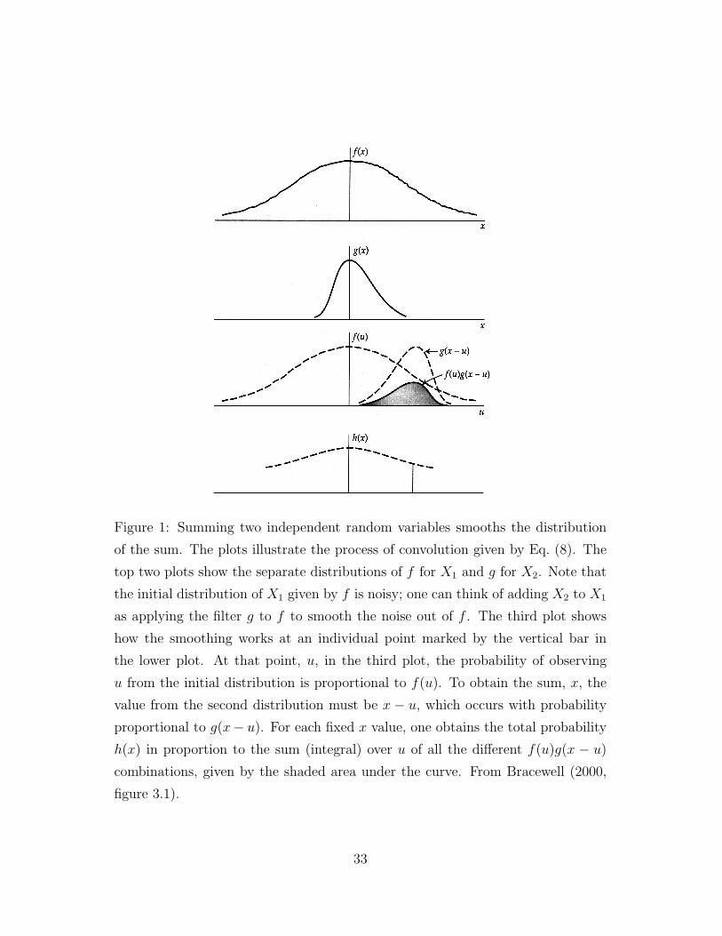
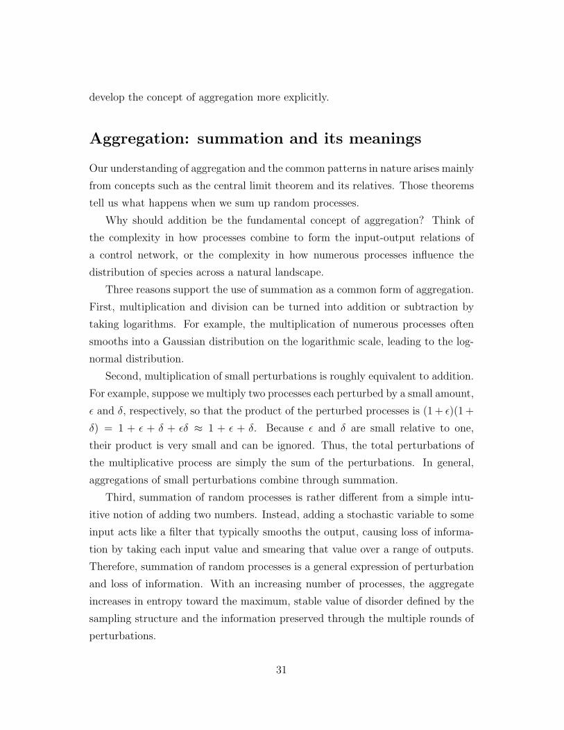
Figure 1: Summing two independent random variables smooths the distribution
of the sum. The plots illustrate the process of convolution given by Eq. (8). The
top two plots show the separate distributions of f for X1 and g for X2. Note that
the initial distribution of X1 given by f is noisy; one can think of adding X2 to X1
as applying the filter g to f to smooth the noise out of f . The third plot shows
how the smoothing works at an individual point marked by the vertical bar in
the lower plot. At that point, u, in the third plot, the probability of observing
u from the initial distribution is proportional to f(u). To obtain the sum, x, the
value from the second distribution must be x − u, which occurs with probability
proportional to g(x− u). For each fixed x value, one obtains the total probability
h(x) in proportion to the sum (integral) over u of all the different f(u)g(x − u)
combinations, given by the shaded area under the curve. From Bracewell (2000,
figure 3.1).
33
Figure 2: Another example of how summing random variables (convolution)
smooths a distribution. The top plots show the initial noisy distribution f and a
second, smoother distribution, g. The distribution of the sum, h = f ∗ g, smooths
the initial distribution of f . The middle plot shows a piece of f broken into in-
tervals, highlighting two intervals x = x1 and x = x2. The lower panel shows
how convolution of f and g gives the probability, h(x), that the sum takes on a
particular value, x. For example, the value h(x1) is the shaded area under the left
curve, which is the sum (integral) of f(u)g(x − u) over all values of u and then
evaluated at x = x1. The area under the right curve is h(x2) obtained by the same
calculation evaluated at x = x2. From Bracewell (2000, figures 3.2 and 3.3).
34
The Fourier transform: the key to aggregation and pattern
The previous section emphasized that aggregation often sums random fluctuations.
If we sum two independent random processes, Y2 = X1 + X2, each drawn from
the same distribution, f(x), then the distribution of the sum is the convolution
of f with itself: g(x) = f ∗ f = f ∗2. Similarly, if we summed n independent
observations from the same distribution,
Yn =n∑i=1
Xi, (10)
then g(x), the distribution of Yn, is the n-fold convolution g(x) = f ∗n. Thus, it
is very easy, in principle, to calculate the distribution of a sum of independent
random fluctuations. However, convolution given by Eq. (8) is tedious and does
not lead to easy analysis.
Fourier transformation provides a useful way to get around the difficulty of
multiple convolutions. Fourier transformation partitions any function into a com-
bination of terms, each term describing the intensity of fluctuation at a particular
frequency. Frequencies are a more natural scale on which to aggregate and study
fluctuations, because weak signals at particular frequencies carry little information
about the true underlying pattern and naturally die away upon aggregation.
To show how Fourier transformation extinguishes weak signals upon aggrega-
tion of random fluctuations, I start with the relation between Fourier transfor-
mation and convolution. The Fourier transform takes some function, f(x), and
changes it into another function, F (s), that contains exactly the same information
but expressed in a different way. In symbols, the Fourier transform is
F{f(x)} = F (s).
The function F (s) contains the same information as f(x), because we can reverse
the process by the inverse Fourier transform
F−1{F (s)} = f(x).
We typically think of x as being any measurement such as time or distance;
the function f(x) may, for example, be the pdf of x, which gives the probability
35

of a fluctuation of magnitude x. In the transformed function, s describes the
fluctuations with regard to their frequencies of repetition at a certain magnitude, x,
and F (s) is the intensity of fluctuations of frequency s. We can express fluctuations
by sine and cosine curves, so that F describes the weighting or intensity of the
combination of sine and cosine curves at frequency s. Thus, the Fourier transform
takes a function f and breaks it into the sum of component frequency fluctuations
with particular weighting F at each frequency s. I give the technical expression of
the Fourier transform at the end of this section.
With regard to aggregation and convolution, we can express a convolution of
probability distributions as the product of their Fourier transforms. Thus, we
can replace the complex convolution operation with multiplication. After we have
finished multiplying and analyzing the transformed distributions, we can transform
back to get a description of the aggregated distribution on the original scale. In
particular, for two independent distributions f(x) and g(x), the Fourier transform
of their convolution is
F{(f ∗ g)(x)} = F (s)G(s).
When we add n independent observations from the same distribution, we must
perform the n-fold convolution, which can also be done by multiplying the trans-
formed function n times
F{f ∗n} = [F (s)]n.
Note that a fluctuation at frequency ω with weak intensity F (ω) will get washed out
compared with a fluctuation at frequency ω′ with strong intensity F (ω′), because
[F (ω)]n
[F (ω′)]n→ 0
with an increase in the number of fluctuations, n, contributing to the aggregate.
Thus the Fourier frequency domain makes clear how aggregation intensifies strong
signals and extinguishes weak signals.
The central limit theorem and the Gaussian distribution
Figure 3 illustrates how aggregation cleans up signals in the the Fourier domain.
The top panel of column (b) in the figure shows the base distribution f(x) for
36
s sx x
(a) FT of sum (b) Sum (c) Normalized sum (d) FT of normalized sum
n
2
4
8
16
1
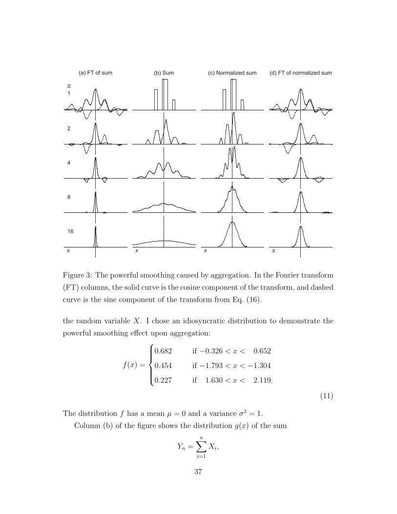
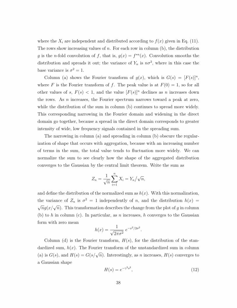
Figure 3: The powerful smoothing caused by aggregation. In the Fourier transform
(FT) columns, the solid curve is the cosine component of the transform, and dashed
curve is the sine component of the transform from Eq. (16).
the random variable X. I chose an idiosyncratic distribution to demonstrate the
powerful smoothing effect upon aggregation:
f(x) =
0.682 if −0.326 < x < 0.652
0.454 if −1.793 < x < −1.304
0.227 if 1.630 < x < 2.119.
(11)
The distribution f has a mean µ = 0 and a variance σ2 = 1.
Column (b) of the figure shows the distribution g(x) of the sum
Yn =n∑i=1
Xi,
37
where the Xi are independent and distributed according to f(x) given in Eq. (11).
The rows show increasing values of n. For each row in column (b), the distribution
g is the n-fold convolution of f , that is, g(x) = f ∗n(x). Convolution smooths the
distribution and spreads it out; the variance of Yn is nσ2, where in this case the
base variance is σ2 = 1.
Column (a) shows the Fourier transform of g(x), which is G(s) = [F (s)]n,
where F is the Fourier transform of f . The peak value is at F (0) = 1, so for all
other values of s, F (s) < 1, and the value [F (s)]n declines as n increases down
the rows. As n increases, the Fourier spectrum narrows toward a peak at zero,
while the distribution of the sum in column (b) continues to spread more widely.
This corresponding narrowing in the Fourier domain and widening in the direct
domain go together, because a spread in the direct domain corresponds to greater
intensity of wide, low frequency signals contained in the spreading sum.
The narrowing in column (a) and spreading in column (b) obscure the regular-
ization of shape that occurs with aggregation, because with an increasing number
of terms in the sum, the total value tends to fluctuation more widely. We can
normalize the sum to see clearly how the shape of the aggregated distribution
converges to the Gaussian by the central limit theorem. Write the sum as
Zn =1√n
n∑i=1
Xi = Yn/√
n,
and define the distribution of the normalized sum as h(x). With this normalization,
the variance of Zn is σ2 = 1 independently of n, and the distribution h(x) =√ng(x/
√n). This transformation describes the change from the plot of g in column
(b) to h in column (c). In particular, as n increases, h converges to the Gaussian
form with zero mean
h(x) =1√
2πσ2e−x
2/2σ2
.
Column (d) is the Fourier transform, H(s), for the distribution of the stan-
dardized sum, h(x). The Fourier transform of the unstandardized sum in column
(a) is G(s), and H(s) = G(s/√n). Interestingly, as n increases, H(s) converges to
a Gaussian shape
H(s) = e−γ2s2 , (12)
38
in which γ2 = σ2/2. The Gaussian is the only distribution which has a Fourier
transform with the same shape.
Maximum entropy in the Fourier domain
The direct and Fourier domains contain the same information. Thus, in deriving
most likely probability distributions subject to the constraints of the information
that we have about a particular problem, we may work equivalently in the direct or
Fourier domains. In the direct domain, we have applied the method of maximum
entropy throughout the earlier sections of this paper. Here, I show the equivalent
approach to maximizing entropy in the Fourier domain.
To obtain the maximum entropy criterion in the Fourier domain (R. W. John-
son & Shore, 1984), we need an appropriate measure of entropy by analogy with
Eq. (1). To get a probability distribution from a Fourier domain function, H(s),
we normalize so that the total area under the Fourier curve is one
H ′(s) = H(s)
/∫ ∞−∞
H(s)ds.
For simplicity, I assume that the direct corresponding distribution, h(x), is centered
at zero and is symmetric, so that H is symmetric and does not have an imaginary
component. If so, then the standardized form of H ′ given here is an appropriate,
symmetric pdf. With a pdf defined over the frequency domain, s, we can apply all
of the standard tools of maximum entropy developed earlier. The corresponding
equation for entropy by reexpressing Eq. (1) is
S = −∫H ′(s) log
[H ′(s)
M(s)
]ds, (13)
where M(s) describes prior information about the relative intensity (probability
distribution) of frequencies, s. Prior information may arise from the sampling
structure of the problem or from other prior information about the relative inten-
sity of frequencies.
With a definition of entropy that matches the standard form used earlier, we
can apply the general solution to maximum entropy problems in Eq. (4), which we
write here as
H ′(s) = kM(s)e−Pλifi , (14)
39
where we choose k so that the total probability is one:∫H ′(s)ds = 1. For the
additional n constraints, we choose each λi so that∫fi(s)H
′(s)ds = 〈fi(s)〉 for
i = 1, 2, . . . , n. For example, if we let f1(s) = s2, then we constrain the second
moment (variance) of the spectral distribution of frequencies. Spectral moments
summarize the location and spread of the power concentrated at various frequencies
(Cramer & Leadbetter, 1967; Benoit et al ., 1992). Here, we can assume M(s) = 1,
because we have no prior information about the spectral distribution. Thus,
H ′(s) = ke−λ1s2 .
We need to choose k so that∫H ′(s)ds = 1 and choose λ1 so that
∫s2H ′(s)ds =
〈s2〉. The identical problem arose when using maximum entropy to derive the
Gaussian distribution in Eq. (7). Here, we have assumed that s is symmetric and
centered at zero, so we can take the mean to be zero, or from Eq. (7), µ = 0. Using
that solution, we have
H ′(s) = ke−s2/2〈s2〉,
where 〈s2〉 is the spectral variance. It turns out that, if we denote the variance of
the direct distribution h(x) as σ2, then 〈s2〉 = 1/σ2; that is, the spectral variance
is the inverse of the direct variance. Here, let us use γ2 = σ2/2 = 1/2〈s2〉, so that
we keep a separate notation for the spectral distribution. Then
H ′(s) = ke−γ2s2 .
The function H ′ is a spectral probability distribution that has been normalized so
that the probability totals to one. However, the actual spectrum of frequencies
in the Fourier domain, H(s), does not have a total area under its curve of one.
Instead the correct constraint for H(s) is that H(0) = 1, which constrains the area
under the probability distribution on the direct scale, h(x), to total to one. If we
choose k = 1, we obtain the maximum entropy solution of spectral frequencies in
the Fourier domain for the probability distribution h(x), subject to a constraint
on the spectral variance γ2 = 1/2〈s2〉, as
H(s) = e−γ2s2 . (15)
If we take the inverse Fourier transform of H(s), we obtain a Gaussian distribu-
tion h(x). This method of spectral maximum entropy suggests that we can use
40

information or assumptions about the spectrum of frequencies in the Fourier do-
main to obtain the most likely probability distributions that describe pattern in
the domain of directly observable measurements.
At first glance, this method of maximum entropy in the frequency domain
may seem unnecessarily complicated. But it turns out that the deepest concepts
of aggregation and pattern can only be analyzed in the frequency domain. The
primacy of the frequency domain may occur because of the natural way in which
aggregation suppresses minor frequencies as noise and enhances major frequencies
as the signals by which information shapes pattern. I develop these points further
after briefly listing some technical details.
Technical details of the Fourier transform
The Fourier transform is given by
F (s) = F{f(x)} =
∫ ∞−∞
f(x)e−ixsdx. (16)
The frequency interpretation via sine and cosine curves arises from the fact that
eis = cos(s) + i sin(s). Thus one can expand the Fourier transform into a series of
sine and cosine components expressed in terms of frequency s.
The inverse transformation demonstrates the full preservation of information
when changing between x and s, given as
f(x) = F−1{F (s)} =1
2π
∫ ∞−∞
F (s)eixsds.
The Levy stable distributions
When we sum variables with finite variance, the distribution of the sum converges
to a Gaussian. Summation is one particular generative process that leads to a
Gaussian. Alternatively, we may consider the distributional problem from an in-
formation perspective. If all we know about a distribution is the variance—the
precision of information in observations with respect to the mean—then the most
likely distribution derived by maximum entropy is Gaussian. From the more gen-
eral information perspective, summation is just one particular generative model
41
that leads to a Gaussian. The generative and information approaches provide dis-
tinct and complementary ways in which to understand the common patterns of
nature.
In this section, I consider cases in which the variance can be infinite. Generative
models of summation converge to a more general form, the Levy stable distribu-
tions. The Gaussian is just a special case of the Levy stable distributions—the
special case of finite variance. From an information perspective, the Levy stable
distributions arise as the most likely pattern given knowledge only about the mo-
ments of the frequency spectrum in the Fourier domain. In the previous section,
I showed that information about the spectral variance leads, by maximum en-
tropy, to the Gaussian distribution. In this section, I show that information about
other spectral moments, such as the mean of the spectral distribution, leads to
other members from the family of Levy stable distributions. The other members,
besides the Gaussian, have infinite variance.
When would the variance be infinite? Perhaps never in reality. More realisti-
cally, the important point is that observations with relatively large values occur
often enough that a set of observations provides very little information about the
average value.
Large variance and the law of large numbers
Consider a random variable X with mean µ and variance σ2. The sum
Zn =1
n
n∑i=1
Xi = X
is the sample mean, X, for a set of n independent observations of the variable X.
If σ2 is finite then, by the central limit theorem, we know that X has a Gaussian
distribution with mean µ and variance σ2/n. As n increases, the variance σ2/n
becomes small, and X converges to the mean µ. We can think of σ2/n, the variance
of X, as the spread of the estimate X about the the true mean, µ. Thus the inverse
of the spread, n/σ2, measures the precision of the estimate. For finite σ2, as n
goes to infinity, the precision n/σ2 also becomes infinite as X converges to µ.
If the variance σ2 is very large, then the precision n/σ2 remains small even as n
42
increases. As long as n does not exceed σ2, precision is low. Each new observation
provides additional precision, or information, about the mean in proportion to
1/σ2. As σ2 becomes very large, the information about the mean per observation
approaches zero.
For example, consider the power law distribution for X with pdf 1/x2 for x > 1.
The probability of observing a value of X greater than k is 1/k. Thus, any new
observation can be large enough to overwhelm all previous observations, no matter
how many observations we have already accumulated. In general, new observations
occasionally overwhelm all previous observations whenever the variance is infinite,
because the precision added by each observation, 1/σ2, is zero. A sum of random
variables, or a random walk, in which any new observation can overwhelm the
information about location in previous observations, is called a Levy flight.
Infinite variance can be characterized by the total probability in the extreme
values, or the tails, of a probability distribution. For a distribution f(x), if the
probability of |x| being greater than k is greater than 1/k2 for large k, then the
variance is infinite. By considering large values of k, we focus on how much prob-
ability there is in the tails of the distribution. One says that when the total
probability in the tails is greater than 1/k2, the distribution has “fat tails,” the
variance is infinite, and a sequence follows a Levy flight.
Variances can be very large in real applications, but probably not infinite.
Below I discuss truncated Levy flights, in which probability distributions have a
lot of weight in the tails and high variance. Before turning to that practical issue,
it helps first to gain full insight into the case of infinite variance. Real cases of
truncated Levy flights with high variance tend to fall between the extremes of the
Gaussian with moderate variance and the Levy stable distributions with infinite
variance.
Generative models of summation
Consider the sum
Zn =1
n1/α
n∑i=1
Xi (17)
43

for independent observations of the random variable X with mean zero. If the
variance of X is finite and equal to σ2, then with α = 2 the distribution of Zn
converges to a Gaussian with mean zero and variance σ2 by the central limit
theorem. In the Fourier domain, the distribution of the Gaussian has Fourier
transform
H(s) = e−γα|s|α (18)
with α = 2, as given in Eq. (12). If α < 2, then the variance of X is infinite,
and the fat tails are given by the total probability 1/|x|α above large values of |x|.The Fourier transform of the distribution of the sum Zn is given by Eq. (18). The
shape of the distribution of X does not matter, as long as the tails follow a power
law pattern.
Distributions with Fourier transforms given by Eq. (18) are called Levy sta-
ble distributions. The full class of Levy stable distributions has a more complex
Fourier transform with additional parameters for the location and skew of the dis-
tribution. The case given here assumes distributions in the direct domain, x, are
symmetric with a mean of zero. We can write the symmetric Levy stable distri-
butions in the direct domain only for α = 2, which is the Gaussian, and for α = 1
which is the Cauchy distribution given by
h(x) =γ
π(γ2 + x2).
As (x/γ)2 increases above about 10, the Cauchy distribution approximately follows
a pdf with a power law distribution 1/|x|1+α, with total probability in the tails
1/|x|α for α = 1.
In general, the particular forms of the Levy stable distributions are known
only from the forms of their Fourier transforms. The fact that the general forms of
these distributions have a simple expression in the Fourier domain occurs because
the Fourier domain is the natural expression of aggregation by summation. In
the direct domain, the symmetric Levy stable distributions approximately follow
power laws with probability 1/|x|1+α as |x|/γ increases beyond a modest threshold
value.
These Levy distributions are called “stable” because they have two properties
that no other distributions have. First, all infinite sums of independent observa-
44
tions from the same distribution converge to a Levy stable distribution. Second,
the properly normalized sum of two or more Levy stable distributions is a Levy
stable distribution of the same form.
These properties cause aggregations to converge to the Levy stable form. Once
an aggregate has converged to this form, combining with another aggregate tends
to keep the form stable. For these reasons, the Levy stable distributions play a
dominant role in the patterns of nature.
Maximum entropy: information and the stable distributions
I showed in Eq. (15) that
H(s) = e−γ2s2
is the maximum entropy pattern in the Fourier domain given information about
the spectral variance. The spectral variance in this case is∫s2H ′(s)ds = 〈s2〉.
If we follow the same derivation for maximum entropy in the Fourier domain,
but use the general expression for the αth spectral moment for α ≤ 2, given by∫|s|αH ′(s)ds = 〈|s|α〉, we obtain the general expression for maximum entropy
subject to information about the αth spectral moment as
H(s) = e−γα|s|α . (19)
This expression matches the general form obtained by n-fold convolution of the
sum in Eq. (17) converging to Eq. (18) by Fourier analysis. The value of α does
not have to be an integer: it can take on any value between 0 and 2. [Here,
γα = 1/α〈|s|α〉, and, in Eq. (14), k = αγ/2Γ(1/a).]
The sum in Eq. (17) is a particular generative model that leads to the Fourier
pattern given by Eq. (18). By contrast, the maximum entropy model uses only
information about the αth spectral moment and derives the same result. The
maximum entropy analysis has no direct tie to a generative model. The maximum
entropy result shows that any generative model or any other sort of information or
assumption that sets the same informational constraints yields the same pattern.
What does the αth spectral moment mean? For α = 2, the moment mea-
sures the variance in frequency when we weight frequencies by their intensity of
45

contribution to pattern. For α = 1, the moment measures the average frequency
weighted by intensity. In general, as α declines, we weight more strongly the lower
frequencies in characterizing the distribution of intensities. Lower frequencies cor-
respond to more extreme values in the direct domain, x, because low frequencies
waves spread more widely. So, as α declines, we weight more heavily the tails of the
probability distribution in the direct domain. In fact, the weighting α corresponds
exactly to the weight in the tails of 1/|x|α for large values of x.
Numerous papers discuss spectral moments (e.g., Benoit et al ., 1992; Eriksson
et al ., 2004). I could find in the literature only a very brief mention of using
maximum entropy to derive Eq. (19) as a general expression of the symmetric Levy
stable distributions (Bologna et al ., 2002). It may be that using spectral moments
in maximum entropy is not considered natural by the physicists who work in this
area. Those physicists have discussed extensively alternative definitions of entropy
by which one may understand the stable distributions (e.g., Abe & Rajagopal,
2000). My own view is that there is nothing unnatural about spectral moments.
The Fourier domain captures the essential features by which aggregation shapes
information.
Truncated Levy flights
The variance is not infinite in practical applications. Finite variance means that
aggregates eventually converge to a Gaussian as the number of the components
in the aggregate increases. Yet many observable patterns have the power law
tails that characterize the Levy distributions that arise as attractors with infinite
variance. Several attempts have been made to resolve this tension between the
powerful attraction of the Gaussian for finite variance and the observable power
law patterns. The issue remains open. In this section, I make a few comments
about the alternative perspectives of generative and informational views.
The generative approach often turns to truncated Levy flights to deal with finite
variance (Mantegna & Stanley, 1994, 1995; Voit, 2005; Mariani & Liu, 2007). In
the simplest example, each observation comes from a distribution with a power
46
law tail such as Eq. (6) with L = 1, repeated here
py = δy−(1+δ),
for 1 ≤ y <∞. The variance of this distribution is infinite. If we truncate the tail
such that 1 ≤ y ≤ U , and normalize so that the total probability is one, we get
the distribution
py =δy−(1+δ)
1− U−δ,
which for large U is essentially the same distribution as the standard power law
form, but with the infinite tail truncated. The truncated distribution has finite
variance. Aggregation of the truncated power law will eventually converge to a
Gaussian. But the convergence takes a very large number of components, and the
convergence can be very slow. For practical cases of finite aggregation, the sum
will often look somewhat like a power law or a Levy stable distribution.
I showed earlier that power laws arise by maximum entropy when one has
information only about 〈log(y)〉 and the lower bound, L. Such distributions have
infinite variance, which may be unrealistic. The assumption that the variance
must be finite means that we must constrain maximum entropy to account for
that assumption. Finite variance implies that 〈y2〉 is finite. We may therefore
consider the most likely pattern arising simply from maximum entropy subject to
the constraints of minimum value, L, geometric mean characterized by 〈log(y)〉,and finite second moment given by 〈y2〉. For this application, we will usually
assume that the second moment is large to preserve the power law character over
most of the range of observations. With those assumptions, our standard procedure
for maximum entropy in Eq. (4) yields the distribution
py = ky−(1+δ)e−γy2
, (20)
where I have here used notation for the λ constants of Eq. (4) with the substitutions
λ1 = 1 + δ and λ2 = γ. No simple expressions give the values of k, δ, and γ; those
values can be calculated from the three constraints:∫pydy = k,
∫y2pydy = 〈y2〉,
and∫
log(y)pydy = 〈log(y)〉. If we assume large but finite variance, then 〈y2〉 is
large and γ will be small. As long as values of γy2 remain much less than one, the
47
distribution follows the standard power law form of Eq. (6). As γy2 grows above
one, the tail of the distribution approaches zero more rapidly than a Gaussian.
I emphasize this informational approach to truncated power laws because it
seems most natural to me. If all we know is a lower bound, L, a power law shape
of the distribution set by δ through the observable range of magnitudes, and a
finite variance, then the form such as Eq. (20) is most likely.
Why are power laws so common?
Because spectral distributions tend to converge to their maximum entropy form
H(s) = e−γα|s|α . (21)
With finite variance, α very slowly tends toward 2, leading to the Gaussian for
aggregations in which component perturbations have truncated fat tails with fi-
nite variance. If the number of components in the aggregate is not huge, then
such aggregates may often closely follow Eq. (21) or a simple power law through
the commonly measurable range of values, as in Eq. (20). Put another way, the
geometric mean often captures most of the information about a process or a set of
data with respect to underlying distribution.
This informational view of power laws does not favor or rule out particular
hypotheses about generative mechanisms. For example, word usage frequencies in
languages might arise by particular processes of preferential attachment, in which
each additional increment of usage is allocated in proportion to current usage. But
we must recognize that any process, in the aggregate, that preserves information
about the geometric mean, and tends to wash out other signals, converges to
a power law form. The consistency of a generative mechanism with observable
pattern tells us little about how likely that generative mechanism was in fact the
cause of the observed pattern. Matching generative mechanism to observed pattern
is particularly difficult for common maximum entropy patterns, which are often
attractors consistent with many distinct generative processes.
48
Extreme value theory
The Levy stable distributions express widespread patterns of nature that arise
through summation of perturbations. Summing logarithms is the same as multi-
plication. Thus, the Levy stable distributions, including the special Gaussian case,
also capture multiplicative interactions.
Extreme values define the other great class of stable distributions that shape
the common patterns of nature. An extreme value is the largest (or smallest) value
from a sample. I focus on largest values. The same logic applies to smallest values.
The cumulative probability distribution function for extreme values, G(x), gives
the probability that the greatest observed value in a large sample will be less than
x. Thus, 1−G(x) gives the probability that the greatest observed value in a large
sample will be higher than x.
Remarkably, the extreme value distribution takes one of three simple forms.
The particular form depends only on the shape of the upper tail for the underly-
ing probability distribution that governs each observation. In this section, I give
a brief overview of extreme value theory and its relation to maximum entropy. As
always, I emphasize the key concepts. Several books present full details, mathe-
matical development, and numerous applications (Embrechts et al ., 1997; Kotz &
Nadarajah, 2000; Coles, 2001; Gumbel, 2004).
Applications
Reliability, time to failure, and mortality may depend on extreme values. Sup-
pose an organism or a system depends on numerous components. Failure of any
component causes the system to fail or the organism to die. One can think of
failure for a component as an extreme value in a stochastic process. Then overall
failure depends on how often an extreme value arises in any of the components. In
some cases, overall failure may depend on breakdown of several components. The
Weibull distribution is often used to describe these kinds of reliability and failure
problems (Juckett & Rosenberg, 1992). We will see that the Weibull is one of the
three general types of extreme value distributions.
Many problems in ecology and evolution depend on evaluating rare events.
49
What is the risk of invasion by a pest species (Franklin et al ., 2008)? For an
endangered species, what is the risk of rare environmental fluctuations causing
extinction? What is the chance of a rare beneficial mutation arising in response
to a strong selective pressure (Beisel et al ., 2007)?
General expression of extreme value problems
Suppose we observe a random variable, Y , with a cumulative distribution function,
or cdf, F (y). The cdf is defined as the probability that an observation, Y , is less
than y. In most of this paper, I have focused on the probability distribution
function, or pdf, f(y). The two expressions are related by
P (Y < y) = F (y) =
∫ y
−∞f(x)dx.
The value of F (y) can be used to express the total probability in the lower tail
below y. We often want the total probability in the upper tail above y, which is
P (Y > y) = 1− F (y) = F (y) =
∫ ∞y
f(x)dx,
where I use F for the upper tail probability.
Suppose we observe n independent values Yi from the distribution F . Define
the maximum value among those n observations as Mn. The probability that the
maximum is less than y is equal to the probability that each of the n independent
observations is less than y, thus
P (Mn < y) = [F (y)]n.
This expression gives the extreme value distribution, because it expresses the prob-
ability distribution of the maximum value. The problem is that, for large n,
[F (y)]n → 0 if F (y) < 1 and [F (y)]n → 1 if F (y) = 1. In addition, we often do
not know the particular form of F . For a useful analysis, we want to know about
the extreme value distribution without having to know exactly the form of F , and
we want to normalize the distribution so that it approaches a limiting value as
n increases. We encountered normalization when studying sums of random vari-
ables: without normalization, a sum of n observations often grows infinitely large
50
as n increases. By contrast, a properly normalized sum converges to a Levy stable
distribution.
For extreme values, we need to find a normalization for the maximum value in
a sample of size n, Mn, such that
P [(Mn − bn)/an < y]→ G(y). (22)
In words, if we normalize the maximum, Mn, by subtracting a location coefficient,
bn, and dividing by a scaling coefficient, an, then the extreme value distribution
converges to G(y) as n increases. Using location and scale coefficients that depend
on n is exactly what one does in normalizing a sum to obtain the standard Gaussian
with mean zero and standard deviation one: in the Gaussian case, to normalize a
sum of n observations, one subtracts from the sum bn = nµ, and divides the sum by√nσ, where µ and σ are the mean and standard deviation of the distribution from
which each observation is drawn. The concept of normalization for extreme values
is the same, but the coefficients differ, because we are normalizing the maximum
value of n observations rather than the sum of n observations.
We can rewrite our extreme value normalization in Eq. (22) as
P (Mn < any + bn)→ G(y).
Next we use the equivalences established above to write
P (Mn < any + bn) =[F (any + bn)
]n=[1− F (any + bn)
]n.
We note a very convenient mathematical identity(1− F (y)
n
)n→ e−F (y)
as n becomes large. Thus, if we can find values of an and bn such that
F (any + bn) =F (y)
n, (23)
then we obtain the general solution for the extreme value problem as
G(y) = e−F (y), (24)
51
where F (y) is the probability in the upper tail for the underlying distribution of
the individual observations. Thus, if we know the shape of the upper tail of Y ,
and we can normalize as in Eq. (23), we can express the distribution for extreme
values, G(y).
The tail determines the extreme value distribution
I give three brief examples that characterize the three different types of extreme
value distributions. No other types exist (Embrechts et al ., 1997; Kotz & Nadara-
jah, 2000; Coles, 2001; Gumbel, 2004).
In the first example, suppose the upper tail of Y decreases exponentially such
that F (y) = e−y. Then, in Eq. (23), using an = 1 and bn = − log(n), from Eq. (24),
we obtain
G(y) = e−e−y, (25)
which is called the double exponential or Gumbel distribution. Typically any dis-
tribution with a tail that decays faster than a power law attracts to the Gumbel,
where, by Eq. (6), a power law has a total tail probability in its cumulative dis-
tribution function proportional to 1/yδ, with δ < 2. Exponential, Gaussian, and
gamma distributions all decay exponentially with tail probabilities less than power
law tail probabilities.
In the second example, let the upper tail of Y decrease like a power law such
that F (y) = y−δ. Then, with an = n1/δ and bn = 0, we obtain
G(y) = e−y−δ, (26)
which is called the Frechet distribution.
Finally, if Y has a finite maximum value M such that F (y) has a truncated
upper tail, and the tail probability near the truncation point is F (y) = (M − y)δ,
then, with an = n−1/δ and bn = n−1/δM −M , we obtain
G(y) = e−(M−y)δ , (27)
which is called the Weibull distribution. Note that G(y) = 0 for y > M , because
the extreme value can never be larger than the upper truncation point.
52
Maximum entropy: what information determines extreme values?
In this section, I show the constraints that define the maximum entropy patterns
for extreme values. Each pattern arises from two constraints. One constraint
sets the average location either by the mean, 〈y〉, for cases with exponential tail
decay, or by the geometric mean measured by 〈log(y)〉 for power law tails. To
obtain a general form, express this first constraint as 〈ξ(y)〉, where ξ(y) = y or
ξ(y) = log(y). The other constraint measures the average tail weighting, 〈F (y)〉.With the two constraints 〈ξ(y)〉 and 〈F (y)〉, the maximum entropy probability
distribution (pdf) is
g(y) = ke−λ1ξ(y)−λ2F (y). (28)
We can relate this maximum entropy probability distribution function (pdf) to the
results for the three types of extreme value distributions. I gave the extreme value
distributions as G(y), the cumulative distribution function (cdf). We can obtain
the pdf from the cdf by differentiation, because g(y) = dG(y)/dy.
From Eq. (25), the pdf of the Gumbel distribution is
g(y) = e−y−e−y,
which, from Eq. (28), corresponds to a constraint 〈ξ(y)〉 = 〈y〉 for the mean and
a constraint 〈F (y)〉 = 〈e−y〉 for the exponentially weighted tail shape. Here,
k = λ1 = λ2 = 1.
From Eq. (26), the pdf of the Frechet distribution is
g(y) = δy−(1+δ)e−y−δ,
which, from Eq. (28), corresponds to a constraint 〈ξ(y)〉 = 〈log(y)〉 for the geo-
metric mean and a constraint 〈F (y)〉 = 〈y−δ〉 for power law weighted tail shape.
Here, k = δ, λ1 = 1 + δ, and λ2 = 1.
From Eq. (27), the pdf of the Weibull distribution is
g(y) = δ(M − y)δ−1e−(M−y)δ ,
which, from Eq. (28), corresponds to a constraint 〈ξ(y)〉 = 〈log(y)〉 for the geo-
metric mean and a constraint 〈F (y)〉 = 〈(M − y)δ〉 that weights extreme values
by a truncated tail form. Here, k = δ, λ1 = 1− δ, and λ2 = 1.
53

In summary, Eq. (28) provides a general form for extreme value distributions.
As always, we can think of that maximum entropy form in two complementary
ways. First, aggregation by repeated sampling suppresses weak signals and en-
hances strong signals until the only remaining information is contained in the
location and in the weighting function constraints. Second, independent of any
generative process, if we use measurements or extrinsic information to estimate or
assume location and weighting function constraints, then the most likely distribu-
tion given those constraints takes on the general extreme value form.
Generative models versus information constraints
The derivations in the previous section followed a generative model in which one
obtains n independent observations from the same underlying distribution. As
n increases, the extreme value distributions converge to one of three forms, the
particular form depending on the tail of the underlying distribution.
We have seen several times in this paper that such generative models often
attract to very general maximum entropy distributions. Those maximum entropy
distributions also tend to attract a wide variety of other generative processes.
In the extreme value problem, any underlying distributions that share similar
probability weightings in the tails fall within the domain of attraction to one of
the three maximum entropy extreme value distributions (Embrechts et al ., 1997).
In practice, one often first discovers a common and important pattern by a
simple generative model. That generative model aggregates observations drawn in-
dependently from a simple underlying distribution that may be regarded as purely
random or neutral. It is, however, a mistake to equate the neutral generative
model with the maximum entropy pattern that it creates. Maximum entropy pat-
terns typically attract a very wide domain of generative processes. The attraction
to simple maximum entropy patterns arises because those patterns express sim-
ple informational constraints and nothing more. Aggregation inevitably washes
out most information by the accumulation of partially uncorrelated perturbations.
What remains in any aggregation is the information in the sampling structure, the
invariance to changes in measurement scale, and the few signals retained through
54
aggregation. Those few bits of information define the common patterns of nature.
Put another way, the simple generative models can be thought of as tools by
which we discover important maximum entropy attractor distributions. Once we
have found such distributions by a generative model, we may extract the informa-
tional constraints that define the pattern. With that generalization in hand, we
can then consider the broad scope of alternative generative processes that preserve
the information that defines the pattern. The original generative model no longer
has special status—our greatest insight resides with the informational constraints
that define the maximum entropy distribution.
The challenge concerns how to use knowledge of the common patterns to draw
inferences about pattern and process in biology. This paper has been about the
first step: to understand clearly how information defines the relations between
generative models of process and the consequences for pattern. I only gave the
logical structure rather than direct analyses of important biological patterns. The
next step requires analysis of the common patterns in biology with respect to
sampling structure, informational constraints, and the domains of attraction for
generative models to particular patterns. What range of non-neutral generative
models attract to the common patterns, because the extra non-neutral information
gets washed out with aggregation?
With the common patterns of biology better understood, one can then analyze
departures from the common patterns more rationally. What extra information
causes departures from the common patterns? Where does the extra information
come from? What is it about the form of aggregation that preserves the extra
information? How are evolutionary dynamics and biological design influenced by
the tendency for aggregates to converge to a few common patterns?
Acknowledgments
I came across the epigraph from Gnedenko and Kolmogorov in Sornette (2006)
and the epigraph from Galton in Hartl (2000). My research is supported by Na-
tional Science Foundation grant EF-0822399, National Institute of General Medi-
cal Sciences MIDAS Program grant U01-GM-76499, and a grant from the James
55

S. McDonnell Foundation.
56
References
Abe, S. & Rajagopal, A. K. 2000. Justification of power law canonical distributions
based on the generalized central-limit theorem. Europhys. Lett. 52: 610-614.
Barabasi, A. L. & Albert, R. 1999. Emergence of scaling in random networks.
Science 286: 509-512.
Beisel, C. J., Rokyta, D. R., Wichman, H. A. & Joyce, P. 2007. Testing the ex-
treme value domain of attraction for distributions of beneficial fitness effects.
Genetics 176: 2441-2449.
Benoit, C., Royer, E. & Poussigue, G. 1992. The spectral moments method. J.
Phys.-Condens. Mat. 4: 3125-3152.
Bologna, M., Campisi, M. & Grigolini, P. 2002. Dynamic versus thermodynamic
approach to non-canonical equilibrium. Physica A 305: 89-98.
Bracewell, R. N. 2000. The Fourier Transform and its Applications 3rd edn.
McGraw Hill, Boston.
Coles, S. 2001. An Introduction to Statistical Modeling of Extreme Values.
Springer, New York.
Cramer, H. & Leadbetter, M. R. 1967. Stationary and Related Stochastic Processes:
Sample Function Properties and their Applications. Wiley, New York.
Embrechts, P., Kluppelberg, C. & Mikosch, T. 1997. Modeling Extremal Events:
For Insurance and Finance. Springer Verlag, Heidelberg.
Eriksson, E. J., Cepeda, L. F., Rodman, R. D., Sullivan, K. P. H., McAllister,
D. F., Bitzer, D. et al . 2004. Robustness of spectral moments: a study
using voice imitations. Proceedings of the Tenth Australian International
Conference on Speech Science and Technology 1: 259-264.
Feller, W. 1968. An Introduction to Probability Theory and its Applications 3rd
edn, Vol. I. Wiley, New York.
Feller, W. 1971. An Introduction to Probability Theory and its Applications 2nd
edn, Vol. II. Wiley, New York.
Franklin, J., Sisson, S. A., Burgman, M. A. & Martin, J. K. 2008. Evaluating
extreme risks in invasion ecology: learning from banking compliance. Divers.
Distrib. 14: 581-591.
57
Galton, F. 1889. Natural Inheritance. MacMillan, London and New York.
Garcia Martin, H. & Goldenfeld, N. 2006. On the origin and robustness of power-
law species-area relationships in ecology. P. Natl. Acad. Sci. USA 103:
10310-10315.
Gnedenko, B. V. & Kolmogorov, A. N. 1968. Limit Distributions for Sums of
Independent Random Variables. Addison-Wesley, Reading, MA.
Gumbel, E. J. 2004. Statistics of Extremes. Dover Publications, New York.
Hall, P. & Heyde, C. C. 1980. Martingale Limit Theory and its Application.
Academic Press, New York.
Hartl, D. L. 2000. A Primer of Population Genetics 3rd edn. Sinauer, Sanderland,
MA.
Jaynes, E. T. 2003. Probability Theory: The Logic of Science. Cambridge Univer-
sity Press, New York.
Johnson, N. L., Kemp, A. W. & Kotz, S. 2005. Univariate Discrete Distributions
3rd edn. Wiley, Hoboken, NJ.
Johnson, N. L., Kotz, S. & Balakrishnan, N. 1994. Continuous Univariate Distri-
butions 2nd edn. Wiley, New York.
Johnson, O. 2004. Information Theory and the Central Limit Theorem. Imperial
College Press, London.
Johnson, R. W. & Shore, J. E. 1984. Which is the better entropy expression for
speech processing: -S log S or log S? IEEE T. Acoust. Speech. 32: 129-137.
Juckett, D. A. & Rosenberg, B. 1992. Human disease mortality kinetics are
explored through a chain model embodying principles of extreme value theory
and competing risks. J. Theor. Biol. 155: 463-483.
Kapur, J. N. 1989. Maximum-entropy Models in Science and Engineering. Wiley,
New York.
Kleiber, C. & Kotz, S. 2003. Statistical Size Distributions in Economics and
Actuarial Sciences. Wiley, New York.
Kotz, S. & Nadarajah, S. 2000. Extreme Value Distributions: Theory and Appli-
cations. World Scientific, Singapore.
Kullback, S. 1959. Information Theory and Statistics. Wiley, New York.
Mandelbrot, B. B. 1983. The Fractal Geometry of Nature. WH Freeman, New
58
York.
Mantegna, R. N. & Stanley, H. E. 1994. Stochastic process with ultraslow con-
vergence to a Gaussian: The truncated Levy flight. Phys. Rev. Lett. 73:
2946-2949.
Mantegna, R. N. & Stanley, H. E. 1995. Scaling behaviour in the dynamics of an
economic index. Nature 376: 46-49.
Mariani, M. C. & Liu, Y. 2007. Normalized truncated Levy walks applied to the
study of financial indices. Physica A 377: 590-598.
Mitzenmacher, M. 2004. A brief history of generative models for power law and
lognormal distributions. Internet Math. 1: 226-251.
Newman, M. E. J. 2005. Power laws, Pareto distributions and Zipf’s law. Contemp.
Phys. 46: 323.
Ravasz, E., Somera, A. L., Mongru, D. A., Oltvai, Z. N. & Barabasi, A. L. 2002.
Hierarchical organization of modularity in metabolic networks. Science 297:
1551-1555.
Shannon, C. E. & Weaver, W. 1949. The Mathematical Theory of Communication.
University of Illionis Press, Urbana, IL.
Simkin, M. V. & Roychowdhury, V. P. 2006. Re-inventing Willis.
Arxiv:physics/0601192 : .
Simon, H. A. 1955. On a class of skew distribution functions. Biometrika 42:
425-440.
Sivia, D. S. & Skilling, J. 2006. Data Analysis: A Bayesian Tutorial. Oxford
University Press, New York.
Sornette, D. 2006. Critical Phenomena in Natural Sciences: Chaos, Fractals,
Selforganization, and Disorder: Concepts and Tools. Springer, New York.
Stigler, S. M. 1986. The History of Statistics: The Measurement of Uncertainty
before 1900. Belknap Press of Harvard University Press, Cambridge, MA.
Tribus, M. 1961. Thermostatics and Thermodynamics: An Introduction to En-
ergy, Information and States of Matter, with Engineering Applications. Van
Nostrand, New York.
Tsallis, C. 1988. Possible generalization of Boltzmann-Gibbs statistics. J. Stat.
Phys. 52: 479-487.
59
Tsallis, C. 1999. Nonextensive statistics: Theoretical, experimental and compu-
tational evidences and connections. Braz. J. Phys. 29: 1-35.
Van Campenhout, J. M. & Cover, T. M. 1981. Maximum entropy and conditional
probability. IEEE Trans. Inform. Theory 27: 483-489.
Voit, J. 2005. The Statistical Mechanics of Financial Markets 3rd edn. Springer,
New York.
Yu, Y. M. 2008. On the maximum entropy properties of the binomial distribution.
IEEE Trans. Inform. Theory 54: 3351-3353.
60
Related Documents