The Combinatorial Revolution in Knot Theory Sam Nelson K not theory is usually understood to be the study of embeddings of topologi- cal spaces in other topological spaces. Classical knot theory, in particular, is concerned with the ways in which a cir- cle or a disjoint union of circles can be embedded in R 3 . Knots are usually described via knot dia- grams, projections of the knot onto a plane with breaks at crossing points to indicate which strand passes over and which passes under, as in Fig- ure 1. However, much as the concept of “numbers” has evolved over time from its original meaning of cardinalities of finite sets to include ratios, equivalence classes of rational Cauchy sequences, roots of polynomials, and more, the classical con- cept of “knots” has recently undergone its own evolutionary generalization. Instead of thinking of knots topologically as ambient isotopy classes of embedded circles or geometrically as simple closed curves in R 3 , a new approach defines knots combinatorially as equivalence classes of knot di- agrams under an equivalence relation determined by certain diagrammatic moves. No longer merely symbols standing in for topological or geomet- ric objects, the knot diagrams themselves have become mathematical objects of interest. Doing knot theory in terms of knot diagrams, of course, is nothing new; the Reidemeister moves date back to the 1920s [21], and identifying knot invariants (functions used to distinguish differ- ent knot types) by checking invariance under the moves has been common ever since. A recent shift toward taking the combinatorial approach more Sam Nelson is assistant professor of mathematics at Clare- mont McKenna College, a member of the Claremont Uni- versity Consortium in Claremont, CA. His email address is [email protected]. Figure 1. Knot diagrams. seriously, however, has led to the discovery of new types of generalized knots and links that do not correspond to simple closed curves in R 3 . Like the complex numbers arising from missing roots of real polynomials, the new generalized knot types appear as abstract solutions in knot equations that have no solutions among the classi- cal geometric knots. Although they seem esoteric at first, these generalized knots turn out to have interpretations such as knotted circles or graphs in three-manifolds other than R 3 , circuit diagrams, and operators in exotic algebras. Moreover, clas- sical knot theory emerges as a special case of the new generalized knot theory. This diagram-based combinatorial approach to knot theory has revived interest in a related approach to algebraic knot invariants, applying techniques from universal algebra to turn the combinatorial structures into algebraic ones. The resulting algebraic objects, with names such as kei, quandles, racks, and biquandles, yield new invari- ants of both classical and generalized knots and provide new insights into old invariants. Much like groups arising from symmetries of geometric ob- jects, these knot-inspired algebraic structures have connections to vector spaces, groups, Lie groups, Hopf algebras, and other mathematical structures. December 2011 Notices of the AMS 1553

Welcome message from author
This document is posted to help you gain knowledge. Please leave a comment to let me know what you think about it! Share it to your friends and learn new things together.
Transcript

The CombinatorialRevolution
in Knot TheorySam Nelson
Knot theory is usually understood to bethe study of embeddings of topologi-cal spaces in other topological spaces.Classical knot theory, in particular, isconcerned with the ways in which a cir-
cle or a disjoint union of circles can be embeddedin R3. Knots are usually described via knot dia-grams, projections of the knot onto a plane withbreaks at crossing points to indicate which strandpasses over and which passes under, as in Fig-ure 1. However, much as the concept of “numbers”has evolved over time from its original meaningof cardinalities of finite sets to include ratios,equivalence classes of rational Cauchy sequences,roots of polynomials, and more, the classical con-cept of “knots” has recently undergone its ownevolutionary generalization. Instead of thinkingof knots topologically as ambient isotopy classesof embedded circles or geometrically as simpleclosed curves in R3, a new approach defines knotscombinatorially as equivalence classes of knot di-agrams under an equivalence relation determinedby certain diagrammatic moves. No longer merelysymbols standing in for topological or geomet-ric objects, the knot diagrams themselves havebecome mathematical objects of interest.
Doing knot theory in terms of knot diagrams,of course, is nothing new; the Reidemeister movesdate back to the 1920s [21], and identifying knotinvariants (functions used to distinguish differ-ent knot types) by checking invariance under themoves has been common ever since. A recent shifttoward taking the combinatorial approach more
Sam Nelson is assistant professor of mathematics at Clare-
mont McKenna College, a member of the Claremont Uni-
versity Consortium in Claremont, CA. His email address
Figure 1. Knot diagrams.
seriously, however, has led to the discovery of
new types of generalized knots and links that do
not correspond to simple closed curves in R3.
Like the complex numbers arising from missing
roots of real polynomials, the new generalized
knot types appear as abstract solutions in knot
equations that have no solutions among the classi-
cal geometric knots. Although they seem esoteric
at first, these generalized knots turn out to have
interpretations such as knotted circles or graphs
in three-manifolds other thanR3, circuit diagrams,
and operators in exotic algebras. Moreover, clas-
sical knot theory emerges as a special case of the
new generalized knot theory.
This diagram-based combinatorial approach to
knot theory has revived interest in a related
approach to algebraic knot invariants, applying
techniques from universal algebra to turn the
combinatorial structures into algebraic ones. The
resulting algebraic objects, with names such as kei,
quandles, racks, and biquandles, yield new invari-
ants of both classical and generalized knots and
provide new insights into old invariants. Much like
groups arising from symmetries of geometric ob-
jects, these knot-inspired algebraic structures have
connections to vector spaces, groups, Lie groups,
Hopf algebras, and other mathematical structures.
December 2011 Notices of the AMS 1553
Consequentially, they have potential applicationsin disciplines from statistical mechanics to bio-chemistry to other areas of mathematics, withmany promising open questions.
Virtual KnotsA geometric knot is a simple closed curve in R3;a geometric link is a union of knots that may belinked together. A diagram D of a knot or linkK is a projection of K onto a plane such that nopoint in D comes from more than two points in K.Every point in the projection with two preimagesis then a crossing point ; if the knot were a physicalrope laid on the plane of the paper, the crossingpoints would be the places where the rope touchesitself. We indicate which strand of the knot goesover and which goes under at a crossing point bydrawing the undercrossing strand with gaps.
Combinatorially, then, a knot or link diagramis a four-valent graph embedded in a plane withvertices decorated to indicate crossing informa-tion. We can describe such a diagram by givinga list of crossings and specifying how the endsare to be connected; for example, a Gauss codeis a cyclically ordered list of over- and under-crossing points with connections determined bythe ordering. See Figure 2.
O1U2O3U1O2U3
Figure 2. A knot and its Gauss code.
Intuitively, moving a knot or link around inspace without cutting or retying it shouldn’tchange the kind of knot or link we have. Thuswe really want topological knots and links, wheretwo geometric knots are topologically equivalent ifone can be continuously deformed into the other.Formally, topological knots are ambient isotopyclasses of geometric knots and links. In the 1920sKurt Reidemeister showed that ambient isotopy ofsimple closed curves in R3 corresponds to equiv-alence of knot diagrams under sequences of themoves in Figure 3 [21]. In these moves, the portionof the diagram outside the pictured neighborhoodremains fixed. The proof that a function definedon knot diagrams is a topological knot invariantis then reduced to a check that the function valueis unchanged by the three moves.
In the mid-1990s various knot theorists (e.g.,[11, 14, 17]), studying combinatorial methods ofcomputing knot invariants using Gauss codes andsimilar schemes for encoding knot diagrams, no-ticed that even the Gauss codes whose associated
Figure 3. Reidemeister moves.
graphs could not be embedded in the plane stillbehaved like knots in certain ways—for instance,knot invariants defined via combinatorial pairingsof Gauss codes still gave valid invariants whenordinary knots were paired with nonplanar Gausscodes. A planar Gauss code always describes asimple closed curve in three-space; what kind ofthing could a nonplanar Gauss code be describing?
Resolving the vertices in a planar four-valentgraph as crossings yields a simple closed curve
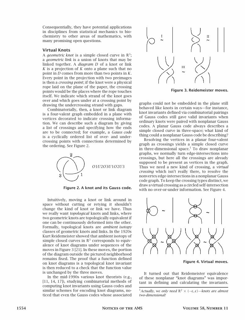
in three-dimensional space.1 To draw nonplanargraphs, we normally turn edge-intersections intocrossings, but here all the crossings are alreadysupposed to be present as vertices in the graph.Thus we need a new kind of crossing, a virtualcrossing which isn’t really there, to resolve thenonvertex edge-intersections in a nonplanar Gausscode graph. To keep the crossing types distinct, wedraw a virtual crossing as a circled self-intersectionwith no over-or-under information. See Figure 4.
Figure 4. Virtual moves.
It turned out that Reidemeister equivalenceof these nonplanar “knot diagrams” was impor-tant in defining and calculating the invariants.
1Actually, we only need R2 × (−ǫ, ǫ)—knots are almost
two-dimensional!
1554 Notices of the AMS Volume 58, Number 11

Since Reidemeister equivalence classes of planar
knot diagrams coincide with classical knots, it
seemed natural to refer to the generalized equiv-
alence classes as “knots” despite their inclusion
of nonplanar diagrams. The computations were
suggesting that familiar topological knots are a
special case of a more general kind of thing,
namely Reidemeister equivalence classes of “knot
diagrams” which may or may not be planar. The re-
sulting “combinatorial revolution” was a shift from
thinking of the diagrams as symbols represent-
ing topological objects (ambient isotopy classes
of simple closed curves in R3) to thinking of the
objects themselves as equivalence classes of dia-
grams. To reject these virtual knots on the grounds
that they do not represent simple closed curves
in R3 would mean throwing away infinite classes
of knot invariants, akin to ignoring complex roots
of polynomials on the grounds that they are not
“real” numbers.
Virtual crossings and their rules of interaction
were introduced in 1996 by Louis Kauffman [17].
Since the virtual crossings are not really there,
any strand with only virtual crossings should
be replaceable with any other strand with the
same endpoints and only virtual crossings. This
is known as the detour move; it breaks down into
the four virtual moves in Figure 4.
Despite their abstract origin, virtual knots do
have a concrete geometric interpretation. Virtual
crossings can be avoided by drawing nonpla-
nar knot diagrams on compact surfaces Σ which
may have nonzero genus,2 providing “bridges”
or “wormholes” that can be used to avoid edge-
crossings. A virtual knot is then a simple closed
curve in an ambient space of the form Σ× (−ǫ, ǫ)(called a thickened surface or trivial I-bundle). Vir-
tual crossings are not crossings in the classical
sense of two strands close together—the strands
meeting in a virtual crossing are on opposite sides
of the ambient space or “universe in which the knot
lives”—but are instead artifacts of forcing a knot
in a nonplanar ambient space into the plane. This
diagrams-on-surfaces approach was introduced
by Naoko and Seiichi Kamada, who dubbed the
results abstract knots in [14]. Other ideas related
to virtual knots conceived independently include
Vladimir Turaev’s virtual strings [24] and Roger
Fenn, Richárd Rimányi, and Colin Rourke’s welded
braids [8].
Figure 5 shows the smallest nonclassical virtual
knot interpreted as a list of labeled crossings
which cannot be realized in the plane, a virtual
knot diagram and a knot diagram drawn on a
surface with nonzero genus.
2Technically, we need to allow stabilization moves on the
surface containing the knot diagram.
Figure 5. A nonclassical virtual knot.
Generalized KnotsOnce we have one new type of crossing, it is naturalto consider others, spawning a zoo of new species
of generalized knot types. Introducing a new kindof crossing requires new Reidemeister-style rulesof interaction. These rules or moves are deter-mined by the desired combinatorial, topological,or geometric interpretation. For example, Figure 6illustrates how the geometric understanding ofvirtual knots as knot diagrams drawn on surfaceswith genus permits some moves while forbidding
others.
∼
6∼
Figure 6. Geometric motivation for moves.
We’ve seen that virtual crossings represent
genus in the surface on which the knot diagram isdrawn. Flat crossings are classical crossings wherewe forget which strand goes over and which goesunder; these are convenient for studying the virtualstructure separately from the classical structureand can be understood as “shadows” of classicalcrossings. Singular crossings are places where theknot is glued to itself with the strands meeting in
a fixed cyclic order, that is, rigid vertices. Knots inI-bundles over nonorientable surfaces are knownas twisted virtual knots; we indicate when a strand
December 2011 Notices of the AMS 1555

has gone through a crosscap with a twist bar [2].
Figure 7 shows generalized crossing types withtheir geometric interpretations, Figure 8 lists someof their interaction laws, and Figure 9 shows some
forbidden moves that look plausible but are notallowed based on the topological motivations for
the new crossing types.
Virtual
Flat
Singular
Twist bar
Figure 7. Generalized crossing types.
The combinatorial revolution also applies tohigher-dimensional knots. Knotted surfaces in R4
have “diagrams” consisting of immersed surfaces
inR3 with sheets broken to indicate crossing infor-mation. Combinatorially, such a knotted surfacediagram consists of boxes containing triple points,
boxes containing cone points, boxes containingpairs of crossed sheets, and boxes containing sin-gle sheets, each with information about how the
boxes are to be connected. An abstract knottedsurface diagram allows joining boxes in arbitraryways, including ways that require virtual self-
intersections to fit into R3. An abstract knotted
surface is then an equivalence class of such di-agrams under the Roseman moves, the knotted
surface version of the Reidemeister moves [4].Introducing new types of crossings is not the
only way to combinatorially generalize knots;
much as altering the rules of arithmetic canchange Z into Zn, changing the list of allowed
moves by replacing a move or adding or delet-ing moves also results in new types of “knots”,
in which we now understand the term “knot” tomean “equivalence class of diagrams”. As withthe generalized crossing types, such alternativemove-sets usually have a geometric or topologi-cal motivation. One example is framed knots, inwhich the geometric notion of fixing the linkingnumber of the knot with its blackboard framingcurve corresponds combinatorially to replacingthe type I move with a writhe-preserving doubled Imove, illustrated in Figure 10. Another exampleis welded knots, in which a strand may move overbut not under a virtual crossing; welded virtualcrossings are pictured as “welded to the paper”.
Generalized knots have unusual properties notfound in the classical knot world. Flipping a virtualknot over, that is, viewing it from the other side ofthe paper, generally results in a different virtual
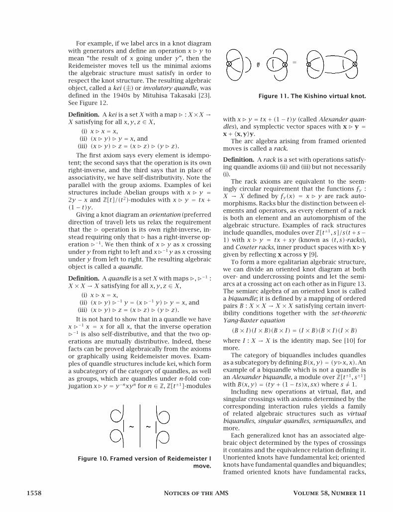
knot,3 unlike the classical case in which flippingover is just a rotation in space. Similarly, we can tietwo virtual unknots sequentially in a string and geta nontrivial knot as a result! Figure 11 shows theKishino knot, the result of joining two trivial virtualknots to obtain a nontrivial virtual knot [19]. Thereader is invited to verify that the two knots onthe left are trivial and to try to unknot the virtualknot on the right using only the legal moves fromFigures 3 and 4 and not the forbidden moves inFigure 9. Proving that the Kishino knot is nontrivialturned out to be quite difficult, requiring algebraicinvariants such as those in the next section.
Despite their apparent strangeness, generalizedknots are increasingly finding applications bothinside and outside of knot theory. Every invariantof virtual knots is automatically an invariant ofordinary classical knots. Virtual knot diagramsarise in computations in physics involving nonpla-nar Feynman diagrams [27]. Thinking of degree-nvertices as a type of crossing extends the combi-natorial revolution to spatial graph theory, that is,embeddings of graphs in R3, with applications inmodeling of molecules in biochemistry, as well asareasof theoretical physics, such as spin networks.
Algebraic Knottiness
Turning knots into algebraic structures is an oldidea, relatively speaking; the Artin braid groupswere introduced in the 1920s [1], and manyuseful knot invariants (especially the “quantuminvariants”, which have connections to quantumgroups, i.e., noncommutative noncocommutativeHopf algebras) have been derived from matrix rep-resentations of tangle algebras [15]. Includinggeneralized crossings in our braids and tan-gles naturally yields corresponding new algebraicstructures such as virtual braid groups and flatvirtual tangle algebras, from which generalizedquantum invariants can be derived. However,algebraification of knots via group theory or linear
3Curiously reminiscent of complex conjugation. . . .
1556 Notices of the AMS Volume 58, Number 11

Figure 8. Rules of interaction for generalized crossings.
Figure 9. Forbidden moves.
algebra imposes certain a priori constraints on
the resulting algebraic structures, for example,
associativity of multiplication, which seem some-
how artificial. More importantly, by insisting on
forcing the algebraic structure into a predefined
framework, we risk sacrificing useful information.
The combinatorial diagrammaticviewpoint sug-
gests a method for deriving the minimal algebraic
structure determined by Reidemeister equivalence
of knot diagrams: start by labeling sections of
a knot diagram with generators of an algebraic
structure and defining operations where the pieces
meet at crossings. The Reidemeister moves then
determine axioms for our new algebraic structure.
We can divide the resulting algebraic structures
into arc algebras where the labels are attached to
arcs, that is, portions of the knot diagram from
one undercrossing point to the next (which can
be traced without lifting your pencil), and semiarc
algebras where the generatorsare semiarcs, that is,
portions of the knot diagram obtained by dividing
at both over- and undercrossing points.
December 2011 Notices of the AMS 1557
For example, if we label arcs in a knot diagram
with generators and define an operation x ⊲ y to
mean “the result of x going under y”, then the
Reidemeister moves tell us the minimal axioms
the algebraic structure must satisfy in order to
respect the knot structure. The resulting algebraic
object, called a kei (圭) or involutory quandle, was
defined in the 1940s by Mituhisa Takasaki [23].
See Figure 12.
Definition. A kei is a set X with a map⊲ : X×X →
X satisfying for all x, y, z ∈ X,
(i) x ⊲ x = x,
(ii) (x ⊲ y) ⊲ y = x, and
(iii) (x ⊲ y) ⊲ z = (x ⊲ z) ⊲ (y ⊲ z).
The first axiom says every element is idempo-
tent; the second says that the operation is its own
right-inverse, and the third says that in place of
associativity, we have self-distributivity. Note the
parallel with the group axioms. Examples of kei
structures include Abelian groups with x ⊲ y =
2y − x and Z[t]/(t2)-modules with x ⊲ y = tx +
(1− t)y .
Giving a knot diagram an orientation (preferred
direction of travel) lets us relax the requirement
that the ⊲ operation is its own right-inverse, in-
stead requiring only that ⊲ has a right-inverse op-
eration ⊲−1. We then think of x ⊲ y as x crossing
under y from right to left and x⊲−1y as x crossing
under y from left to right. The resulting algebraic
object is called a quandle.
Definition. A quandle is a setX with maps⊲,⊲−1 :
X ×X → X satisfying for all x, y, z ∈ X,
(i) x ⊲ x = x,
(ii) (x ⊲ y) ⊲−1 y = (x ⊲−1 y) ⊲ y = x, and
(iii) (x ⊲ y) ⊲ z = (x ⊲ z) ⊲ (y ⊲ z).
It is not hard to show that in a quandle we have
x ⊲−1 x = x for all x, that the inverse operation
⊲−1 is also self-distributive, and that the two op-
erations are mutually distributive. Indeed, these
facts can be proved algebraically from the axioms
or graphically using Reidemeister moves. Exam-
ples of quandle structures include kei, which form
a subcategory of the category of quandles, as well
as groups, which are quandles under n-fold con-
jugation x⊲y = y−nxyn for n ∈ Z, Z[t±1]-modules
Figure 10. Framed version of Reidemeister Imove.
=
Figure 11. The Kishino virtual knot.
with x⊲ y = tx+ (1− t)y (called Alexander quan-dles), and symplectic vector spaces with x ⊲ y =
x+ 〈x,y〉y.The arc algebra arising from framed oriented
moves is called a rack.
Definition. A rack is a set with operations satisfy-ing quandle axioms (ii) and (iii) but not necessarily(i).
The rack axioms are equivalent to the seem-ingly circular requirement that the functions fy :X → X defined by fy(x) = x ⊲ y are rack auto-morphisms. Racks blur the distinction between el-ements and operators, as every element of a rackis both an element and an automorphism of thealgebraic structure. Examples of rack structuresinclude quandles, modules over Z[t±1, s]/s(t+ s−1) with x ⊲ y = tx + sy (known as (t, s)-racks),and Coxeter racks, inner product spaces with x⊲y
given by reflecting x across y [9].
To form a more egalitarian algebraic structure,we can divide an oriented knot diagram at bothover- and undercrossing points and let the semi-arcs at a crossing act on each other as in Figure 13.The semiarc algebra of an oriented knot is calleda biquandle; it is defined by a mapping of orderedpairs B : X × X → X × X satisfying certain invert-ibility conditions together with the set-theoreticYang-Baxter equation
(B × I)(I × B)(B × I) = (I × B)(B × I)(I × B)
where I : X → X is the identity map. See [10] formore.
The category of biquandles includes quandlesas a subcategoryby definingB(x, y) = (y⊲x, x). Anexample of a biquandle which is not a quandle isan Alexander biquandle, a module over Z[t±1, s±1]with B(x, y) = (ty + (1− ts)x, sx) where s 6= 1.
Including new operations at virtual, flat, andsingular crossings with axioms determined by thecorresponding interaction rules yields a familyof related algebraic structures such as virtualbiquandles, singular quandles, semiquandles, andmore.
Each generalized knot has an associated alge-braic object determined by the types of crossingsit contains and the equivalence relation defining it.Unoriented knots have fundamental kei; orientedknots have fundamental quandles and biquandles;framed oriented knots have fundamental racks,
1558 Notices of the AMS Volume 58, Number 11
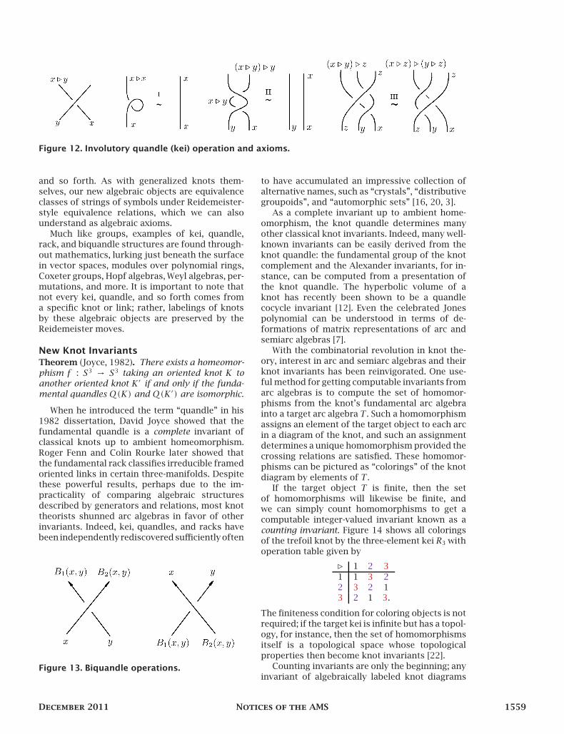
Figure 12. Involutory quandle (kei) operation and axioms.
and so forth. As with generalized knots them-
selves, our new algebraic objects are equivalence
classes of strings of symbols under Reidemeister-
style equivalence relations, which we can alsounderstand as algebraic axioms.
Much like groups, examples of kei, quandle,
rack, and biquandle structures are found through-
out mathematics, lurking just beneath the surface
in vector spaces, modules over polynomial rings,
Coxeter groups, Hopf algebras, Weyl algebras, per-
mutations, and more. It is important to note thatnot every kei, quandle, and so forth comes from
a specific knot or link; rather, labelings of knots
by these algebraic objects are preserved by the
Reidemeister moves.
New Knot InvariantsTheorem (Joyce, 1982). There exists a homeomor-
phism f : S3 → S3 taking an oriented knot K toanother oriented knot K′ if and only if the funda-
mental quandles Q(K) and Q(K′) are isomorphic.
When he introduced the term “quandle” in his
1982 dissertation, David Joyce showed that the
fundamental quandle is a complete invariant of
classical knots up to ambient homeomorphism.
Roger Fenn and Colin Rourke later showed that
the fundamental rack classifies irreducible framed
oriented links in certain three-manifolds. Despitethese powerful results, perhaps due to the im-
practicality of comparing algebraic structures
described by generators and relations, most knot
theorists shunned arc algebras in favor of other
invariants. Indeed, kei, quandles, and racks have
been independently rediscovered sufficiently often
Figure 13. Biquandle operations.
to have accumulated an impressive collection of
alternative names, such as “crystals”, “distributive
groupoids”, and “automorphic sets” [16, 20, 3].
As a complete invariant up to ambient home-
omorphism, the knot quandle determines many
other classical knot invariants. Indeed, many well-
known invariants can be easily derived from the
knot quandle: the fundamental group of the knot
complement and the Alexander invariants, for in-
stance, can be computed from a presentation of
the knot quandle. The hyperbolic volume of a
knot has recently been shown to be a quandle
cocycle invariant [12]. Even the celebrated Jones
polynomial can be understood in terms of de-
formations of matrix representations of arc and
semiarc algebras [7].
With the combinatorial revolution in knot the-
ory, interest in arc and semiarc algebras and their
knot invariants has been reinvigorated. One use-
ful method for getting computable invariants from
arc algebras is to compute the set of homomor-
phisms from the knot’s fundamental arc algebra
into a target arc algebra T . Such a homomorphism
assigns an element of the target object to each arc
in a diagram of the knot, and such an assignment
determines a unique homomorphism provided the
crossing relations are satisfied. These homomor-
phisms can be pictured as “colorings” of the knot
diagram by elements of T .
If the target object T is finite, then the set
of homomorphisms will likewise be finite, andwe can simply count homomorphisms to get a
computable integer-valued invariant known as a
counting invariant. Figure 14 shows all colorings
of the trefoil knot by the three-element kei R3 with
operation table given by
⊲ 1 2 3
1 1 3 22 3 2 13 2 1 3.
The finiteness condition for coloring objects is not
required; if the target kei is infinite but has a topol-
ogy, for instance, then the set of homomorphisms
itself is a topological space whose topological
properties then become knot invariants [22].
Counting invariants are only the beginning; any
invariant of algebraically labeled knot diagrams
December 2011 Notices of the AMS 1559

Figure 14. Kei colorings of the trefoil by R3R3R3.
defines an enhancement of the counting invariant
by taking the multiset of invariant values over the
set of colorings of the knot. One simple example
uses the cardinality of the image subkei of a
kei homomorphism; instead of counting “1” for
each kei homomorphism f : Q(K) → T , we record
t |Im(f )|, obtaining a polynomial invariant
p(t) =∑
f :Q(K)→T
t |Im(f )|,
which has the original counting invariant as p(1).
For example, the trefoil in Figure 14 has counting
invariant 9 with respect toR3 and enhanced invari-
ant p(t) = 3t +6t3. A more sophisticated example
of an enhancement is the family of CJKLS quandle
cocycle invariants which associate a Boltzmann
weight φ(f) with each quandle coloring f , deter-
mined by a cocycle in the second cohomology of
T [5]. In true combinatorial-revolutionary spirit,
such two-cocycles have a geometric interpretation
as virtual link diagrams [4].
Enhancement of counting invariants in which
we replace a cardinality with a set is a basic
example of a more general phenomenon known
as categorification, in which simpler structures
are replaced with higher-powered algebraic struc-
tures. Pioneered by mathematical physicists such
as Louis Crane and John Baez, categorification
involves replacing sets with categories, operations
with functors, and equalities with isomorphisms.
A prime example is Khovanov homology, in which
a combinatorial algorithm for computing the Jones
polynomial from a knot diagram is turned into
a graded chain complex whose Euler character-
istic is the Jones polynomial, with the homology
groups forming a new, stronger invariant [18]. Sim-
ilar methods have been applied to the HOMFLYPT
polynomial and various other quantum knot in-
variants, resulting in new, stronger categorified
knot invariants. This remarkable idea has sparkeda firestorm of new research too vast to adequately
address in this space. Nonetheless, we once again
see the combinatorial revolution in action, as what
was previously merely notation has itself becomea mathematical object of interest.
Not Just for Knot TheoristsWhile arc and semiarc algebras such as quan-
dles and racks have obvious utility in definingknot invariants, fundamentally they are basic al-
gebraic structures analogous to groups or vector
spaces whose potential for applications elsewhere
in mathematics is still largely unexplored. The
fact that groups are first encountered as setsof symmetries does not limit their applications
to geometric rotations and reflections; similarly,
despite their knotty origin, quandles, racks, and
biquandles are likely to have many applications
not tied to knots and links.Starting with a symmetry group, if we take
the subset consisting of only rotations, we get
a subgroup; taking the subset consisting of only
reflections, however, yields not a subgroup but asubkei. Conjugation in a group is a quandle oper-
ation; the resulting conjugation quandles quantify
the failure of commutativity by turning it into
an algebraic structure, analogously to commuta-
tors turning associative algebras into Lie algebras.Indeed, kei, quandles, and racks can be found
lurking wherever operations are noncommutative.
The applications of generalized knots and knot-
inspired algebraic structures are just starting tobe explored, and many open questions remain.
One rich source of project ideas comes from
a simple question: anywhere groups are found,
we can ask what results when we replace the
group with a kei, quandle, or rack. Replacing theknot group with the knot quandle eliminates the
need to worry about the peripheral structure,
for example, and replacing groups with quandles
simplifies monodromy computations analogously[3, 25]. Work is currently under way on the Dehn
quandle of a surface (analogous to the mapping
class group), as well as on quandle and rack
homology, quandle Galois theory, and much more
[26, 6]. What arc algebra structures might belurking in elliptic curves, dynamical systems, or
tensor categories?
Knot diagrams have now come full circle, from
schematic representations of geometric curves in
space to interesting mathematical objects in theirown right. The shift from thinking of knots as
topological to typographical objects gives us new
flexibility and opens the door to new discoveries
1560 Notices of the AMS Volume 58, Number 11

and applications. As was the case with complex
numbers, there has been some resistance to virtual
knot theory from the old guard, though this
author’s subjective impression is that the tide is
turning as more knot theorists embrace the new
generalized knot theory and its related algebraic
structures. In addition to providing new technical
tools for knot theorists and other mathematicians,
generalized knots provide a novel perspective on
what it means to be a knot.
References[1] E. Artin, Theory of braids, Ann. of Math. 48 (1947),
101–126.
[2] M. O. Bourgoin, Twisted link theory, Algebr. Geom.
Topol. 8 (2008), 1249–1279.
[3] E. Brieskorn, Automorphic sets and braids and sin-
gularities, Braids (Santa Cruz, CA, 1986), 45–115,
Contemp. Math. 78, Amer. Math. Soc., Providence,
RI, 1988.
[4] J. Scott Carter, Seiichi Kamada, and Masahico
Saito, Geometric interpretations of quandle ho-
mology, J. Knot Theory Ramifications 10 (2001),
345–386.
[5] J. Scott Carter, Daniel Jelsovsky, Seiichi Ka-
mada, Laurel Langford, and Masahico Saito,
Quandle cohomology and state-sum invariants of
knotted curves and surfaces, Trans. Amer. Math.
Soc. 355 (2003), 3947–3989.
[6] Michael Eisermann, Quandle coverings and their
Galois correspondence, arXiv:math/0612459
[7] , Yang-Baxter deformations of quandles and
racks, Algebr. Geom. Topol. 5 (2005), 537–562.
[8] Roger Fenn, Richárd Rimányi, and Colin
Rourke, The braid-permutation group, Topology
36 (1997), 123–135.
[9] Roger Fenn and Colin Rourke, Racks and links
in codimension two, J. Knot Theory Ramifications 1
(1992), 343–406.
[10] Roger Fenn, Mercedes Jordan-Santana, and
Louis Kauffman, Biquandles and virtual links,
Topology Appl. 145 (2004), 157–175.
[11] Mikhail Goussarov, Michael Polyak, and Oleg
Viro, Finite type invariants of classical and virtual
knots, Topology 39 (2000), 1045–1068.
[12] Ayumu Inoue, Quandle and hyperbolic volume,
arXiv:0812.0425
[13] David Joyce, A classifying invariant of knots, the
knot quandle, J. Pure Appl. Algebra 23 (1982), 37–
65.
[14] Naoko Kamada and Seiichi Kamada, Abstract
link diagrams and virtual knots, J. Knot Theory
Ramifications 9 (2000), 93–106.
[15] Christian Kassel, Quantum Groups, Springer-
Verlag, New York, 1995.
[16] L. H. Kauffman, Knots and Physics, World Scientific
Pub. Co., Singapore (1991 and 1994).
[17] Louis Kauffman, Virtual knot theory, European J.
Combin. 20 (1999), 663–690.
[18] Mikhail Khovanov, A categorification of the Jones
polynomial, Duke Math. J. 101 (2000), 359–426.
[19] Toshimasa Kishino and Shin Satoh, A note
on non-classical virtual knots, J. Knot Theory
Ramifications 13 (2004), 845–856.
[20] S. V. Matveev, Distributive groupoids in knot
theory, Math. USSR Sb. 47 (1984), 73–83.
[21] Kurt Reidemeister, Knotentheorie (reprint),
Springer-Verlag, Berlin-New York, 1974.
[22] Ryszard L. Rubinsztein, Topological quandles and
invariants of links, J. Knot Theory Ramifications 16
(2007), 789–808.
[23] M. Takasaki, Abstractions of symmetric functions,
Tohoku Math. J. 49 (1943), 143–207.
[24] Vladamir Turaev, Virtual strings, Ann. Inst.
Fourier (Grenoble) 54 (2004), 2455–2525.
[25] D. N. Yetter, Quandles and monodromy, J. Knot
Theory Ramifications 12 (2003), 523–541.
[26] Joel Zablow, On relations and homology of the
Dehn quandle, Algebr. Geom. Topol. 8 (2008), 19–51.
[27] Paul Zinn-Justin and Jean-Bernard Zuber, Ma-
trix integrals and the generation and counting
of virtual tangles and links, J. Knot Theory
Ramifications 13 (2004), 325–355.
December 2011 Notices of the AMS 1561
Related Documents