The Characteristic of High-Speed Centrifugal Refrigeration ...

Citation: Hung, K.-S.; Ho, K.-Y.;

Hsiao, W.-C.; Kuan, Y.-D. The

Characteristic of High-Speed

Centrifugal Refrigeration

Compressor with Different

Refrigerants via CFD Simulation.

Processes 2022, 10, 928. https://

doi.org/10.3390/pr10050928

Academic Editor: Weizhong Dai

Received: 31 March 2022

Accepted: 4 May 2022

Published: 7 May 2022

Publisher’s Note: MDPI stays neutral

with regard to jurisdictional claims in

published maps and institutional affil-

iations.

Copyright: © 2022 by the authors.

Licensee MDPI, Basel, Switzerland.

This article is an open access article

distributed under the terms and

conditions of the Creative Commons

Attribution (CC BY) license (https://

creativecommons.org/licenses/by/

4.0/).

processes

Article

The Characteristic of High-Speed Centrifugal RefrigerationCompressor with Different Refrigerants via CFD SimulationKuo-Shu Hung 1, Kung-Yun Ho 2, Wei-Chung Hsiao 2 and Yean-Der Kuan 2,*

1 Green Energy and Environment Research Laboratories, Industrial Technology Research Institute,Hsinchu 31040, Taiwan; [email protected]

2 Department of Refrigeration, Air-Conditioning and Energy Engineering, National Chin-Yi University ofTechnology, Taichung City 41170, Taiwan; [email protected] (K.-Y.H.); [email protected] (W.-C.H.)

* Correspondence: [email protected]; Tel.: +886-4-23924505 (ext. 8256)

Abstract: This study used Computational Fluid Dynamics (CFD) to simulate and analyze the workingfluid in magnetic centrifugal refrigerant compressors using R-134a to mixed refrigerant: R-513A andHFO (Hydrofluoroolefins) Hydrofluoroolefin refrigerant: R-1234yf, and the impact on integratedpart-load performance, Integrated Part Load Value (IPLV) and internal flow field. This study useda single-stage 280 USRT maglev centrifugal refrigerant compressor as a simulation model. Threedifferent refrigerants were used: R-134a, R-513A, and R-1234yf, as presented in the National Instituteof Standards and Technology (NIST) real gas database. The refrigerant was used to set the IPLVworking conditions and change the compressor speed and mass flow rate to simulate the compressor’scharacteristic curve after replacing the refrigerant. The compressor working conditions were thefixed refrigeration cycle condensation and evaporation following the same capacity standards. Thisstudy used the CFD software by Ansys software company to simulate the flow field. The k-omegaturbulence software was used to model the turbulence. The results show that the maglev centrifugalrefrigerant compressor efficiency dropped significantly when the refrigerant was directly replaced.Based on R-134a, the full load efficiency of R-1234yf dropped 13.21%, the full load efficiency of R-513Adropped 9.97%, and the partial load efficiency was similar to R-134a.

Keywords: maglev centrifugal refrigerant compressor; hydrofluoroolefin refrigerant; computationalfluid dynamics

1. Introduction1.1. Development Overview of Magnetic Levitation Centrifugal Compressor

The present magnetic levitation centrifugal compressor has a smaller volume, lowernoise, and lower starting current than conventional centrifugal compressors. The magneticlevitation centrifuge is the most efficient water chiller among the present air-conditioningsystems because the magnetic bearing mechanical loss is much lower than the dynamicbearing mechanical loss. Wide-area volume control is achieved with a frequency converterspeed control, IGV (inlet guide vane), and diffusion width regulation. The small operat-ing range of the conventional fixed-frequency centrifugal compressor is improved. It isconsidered advantageous to replace water chillers with a displacement compressor.

However, the flow field variation inside the centrifugal compressor is complex. Itis difficult to observe the internal flow field variation using instruments. Therefore, thisstudy used CFD to simulate the magnetic levitation centrifugal refrigerant compressorIntegrated Part Load Value (IPLV) using R-134a refrigerant. The simulation result wascompared with the experimental results to validate the simulation result. HFO refrigerantwas replaced with a working fluid for another simulation. This study used R-1234yf andR-513A refrigerant for simulation comparison analyses. The changes in the performanceand flow field of the magnetic levitation centrifugal compressor after replacing the HFCrefrigerant with HFO refrigerant are discussed.

Processes 2022, 10, 928. https://doi.org/10.3390/pr10050928 https://www.mdpi.com/journal/processes

Processes 2022, 10, 928 2 of 21

1.2. Motivation and Objective

There are two methods for replacing the refrigerant: directly replacing the refrigerantand redesigning the compressor for the new refrigerant as shown in Table 1. Directlyreplacing the refrigerant may increase the equipment operation cost, while the redesignmethod will increase the original price of the equipment. This study focused on predictingthe impact of directly replacing the existing R134a refrigerant with R-1234yf refrigerantand R-513A refrigerant. Using the results of this study, it can be judged whether it isnecessary to redesign the compressor blades according to different refrigerants in the future.The purpose is to discuss the effect of direct refrigerant replacement on the high-speedcentrifugal compressor.

Table 1. Cost comparison of direct refrigerant replacement and compressor redesign.

Change Refrigerant Equipment Cost Operating Cost

Direct replacement Low High

Redesign High Low

1.3. Magnetic Levitation Centrifugal Compressor Operating Principle

The magnetic levitation centrifugal compressor drives an impeller to rotate througha magnetic bearing. The refrigerant is sucked into the impeller through an inlet tube andradially delivered at high speed to the diffuser. The fluid’s dynamic energy is reduced by thediffuser and converted into pressure energy. This energy conversion occurs continuouslyat the volute casing. The chiller system’s required pressure ratio and mass flow rate areachieved by high-efficiency impeller compression. The flow field feature and performanceeffectiveness of flow elements are the keys to compressor performance.

In addition to the single-stage compression type magnetic levitation centrifugal com-pressor, this study discussed the compression/pressurization two-stage compression pro-cess. An economizer was arranged between every two compression process stages. Thethermodynamic cycle diagrams are shown in Figure 1.

Processes 2022, 10, x FOR PEER REVIEW 2 of 22

and flow field of the magnetic levitation centrifugal compressor after replacing the HFC refrigerant with HFO refrigerant are discussed.

1.2. Motivation and Objective There are two methods for replacing the refrigerant: directly replacing the refrigerant

and redesigning the compressor for the new refrigerant as shown in Table 1. Directly re-placing the refrigerant may increase the equipment operation cost, while the redesign method will increase the original price of the equipment. This study focused on predicting the impact of directly replacing the existing R134a refrigerant with R-1234yf refrigerant and R-513A refrigerant. Using the results of this study, it can be judged whether it is nec-essary to redesign the compressor blades according to different refrigerants in the future. The purpose is to discuss the effect of direct refrigerant replacement on the high-speed centrifugal compressor.

Table 1. Cost comparison of direct refrigerant replacement and compressor redesign.

Change Refrigerant Equipment Cost Operating Cost Direct replacement Low High

Redesign High Low

1.3. Magnetic Levitation Centrifugal Compressor Operating Principle The magnetic levitation centrifugal compressor drives an impeller to rotate through

a magnetic bearing. The refrigerant is sucked into the impeller through an inlet tube and radially delivered at high speed to the diffuser. The fluid’s dynamic energy is reduced by the diffuser and converted into pressure energy. This energy conversion occurs continu-ously at the volute casing. The chiller system’s required pressure ratio and mass flow rate are achieved by high-efficiency impeller compression. The flow field feature and perfor-mance effectiveness of flow elements are the keys to compressor performance.

In addition to the single-stage compression type magnetic levitation centrifugal com-pressor, this study discussed the compression/pressurization two-stage compression pro-cess. An economizer was arranged between every two compression process stages. The thermodynamic cycle diagrams are shown in Figure 1.

Figure 1. P-h thermodynamic cycle diagrams of single-stage (left) and two-stage (right) centrifugal compressors.

1.4. Magnetic Levitation Centrifugal Compressor Structure The single-stage magnetic levitation centrifugal compressor contains four flow chan-

nel sections: 1. inlet zone, 2. impeller zone, 3. diffuser zone, and 4. volute zone: 1. Inlet zone

Figure 1. P-h thermodynamic cycle diagrams of single-stage (left) and two-stage (right) centrifu-gal compressors.

1.4. Magnetic Levitation Centrifugal Compressor Structure

The single-stage magnetic levitation centrifugal compressor contains four flow channelsections: 1. inlet zone, 2. impeller zone, 3. diffuser zone, and 4. volute zone:

1. Inlet zone

The inlet zone is the area from the compressor inlet to the front end of an impeller.The inlet guide vanes (IGV) can be arranged in the inlet zone annularly, parallel to therefrigerant flow direction when they are not actuating. When the refrigerant flow needs to

Processes 2022, 10, 928 3 of 21

be reduced, the flow direction of the fluid entering the impeller is controlled by changingthe blade angle. The fluid is pre-rotated to control the flow and regulate the refrigeratingcapacity in the water chiller. The inlet zone is free of IGV in this study, and the inlet nozzlewas used instead.

2. Impeller zone

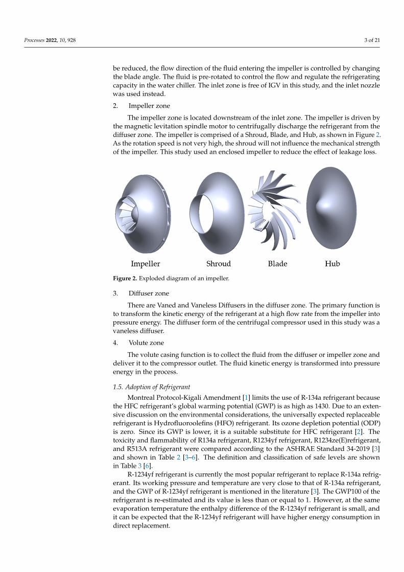
The impeller zone is located downstream of the inlet zone. The impeller is driven bythe magnetic levitation spindle motor to centrifugally discharge the refrigerant from thediffuser zone. The impeller is comprised of a Shroud, Blade, and Hub, as shown in Figure 2.As the rotation speed is not very high, the shroud will not influence the mechanical strengthof the impeller. This study used an enclosed impeller to reduce the effect of leakage loss.

Processes 2022, 10, x FOR PEER REVIEW 3 of 22

The inlet zone is the area from the compressor inlet to the front end of an impeller. The inlet guide vanes (IGV) can be arranged in the inlet zone annularly, parallel to the refrigerant flow direction when they are not actuating. When the refrigerant flow needs to be reduced, the flow direction of the fluid entering the impeller is controlled by chang-ing the blade angle. The fluid is pre-rotated to control the flow and regulate the refriger-ating capacity in the water chiller. The inlet zone is free of IGV in this study, and the inlet nozzle was used instead. 2. Impeller zone

The impeller zone is located downstream of the inlet zone. The impeller is driven by the magnetic levitation spindle motor to centrifugally discharge the refrigerant from the diffuser zone. The impeller is comprised of a Shroud, Blade, and Hub, as shown in Figure 2. As the rotation speed is not very high, the shroud will not influence the mechanical strength of the impeller. This study used an enclosed impeller to reduce the effect of leak-age loss.

Figure 2. Exploded diagram of an impeller.

3. Diffuser zone There are Vaned and Vaneless Diffusers in the diffuser zone. The primary function

is to transform the kinetic energy of the refrigerant at a high flow rate from the impeller into pressure energy. The diffuser form of the centrifugal compressor used in this study was a vaneless diffuser. 4. Volute zone

The volute casing function is to collect the fluid from the diffuser or impeller zone and deliver it to the compressor outlet. The fluid kinetic energy is transformed into pres-sure energy in the process.

1.5. Adoption of Refrigerant Montreal Protocol-Kigali Amendment [1] limits the use of R-134a refrigerant because

the HFC refrigerant’s global warming potential (GWP) is as high as 1430. Due to an exten-sive discussion on the environmental considerations, the universally expected replaceable refrigerant is Hydrofluoroolefins (HFO) refrigerant. Its ozone depletion potential (ODP) is zero. Since its GWP is lower, it is a suitable substitute for HFC refrigerant [2]. The toxicity and flammability of R134a refrigerant, R1234yf refrigerant, R1234ze(E)refrigerant, and R513A refrigerant were compared according to the ASHRAE Standard 34-2019 [3] and shown in Table 2 [3–6]. The definition and classification of safe levels are shown in Table 3 [6].

Figure 2. Exploded diagram of an impeller.

3. Diffuser zone

There are Vaned and Vaneless Diffusers in the diffuser zone. The primary function isto transform the kinetic energy of the refrigerant at a high flow rate from the impeller intopressure energy. The diffuser form of the centrifugal compressor used in this study was avaneless diffuser.

4. Volute zone

The volute casing function is to collect the fluid from the diffuser or impeller zone anddeliver it to the compressor outlet. The fluid kinetic energy is transformed into pressureenergy in the process.

1.5. Adoption of Refrigerant

Montreal Protocol-Kigali Amendment [1] limits the use of R-134a refrigerant becausethe HFC refrigerant’s global warming potential (GWP) is as high as 1430. Due to an exten-sive discussion on the environmental considerations, the universally expected replaceablerefrigerant is Hydrofluoroolefins (HFO) refrigerant. Its ozone depletion potential (ODP)is zero. Since its GWP is lower, it is a suitable substitute for HFC refrigerant [2]. Thetoxicity and flammability of R134a refrigerant, R1234yf refrigerant, R1234ze(E)refrigerant,and R513A refrigerant were compared according to the ASHRAE Standard 34-2019 [3]and shown in Table 2 [3–6]. The definition and classification of safe levels are shownin Table 3 [6].

R-1234yf refrigerant is currently the most popular refrigerant to replace R-134a refrig-erant. Its working pressure and temperature are very close to that of R-134a refrigerant,and the GWP of R-1234yf refrigerant is mentioned in the literature [3]. The GWP100 of therefrigerant is re-estimated and its value is less than or equal to 1. However, at the sameevaporation temperature the enthalpy difference of the R-1234yf refrigerant is small, andit can be expected that the R-1234yf refrigerant will have higher energy consumption indirect replacement.

Processes 2022, 10, 928 4 of 21

Table 2. Refrigerant properties [3–6].

Refrigerant R134a R1234yf R1234ze(E) R513A

Type HFC-134a HFO-1234yf HFO-1234ze HFO-1234yf/HFC-134a (56/44)

Molar Mass (kg/kmol) 102.032 114.042 114.04 108.43

Critical Temperature (K) 374.26 367.85 382.51 368.06

Critical Pressure (kPa) 4059 3382.2 3634.9 3647.8

Critical Volume (m3/mol) 2.008 × 10−4 2.39808 × 10−4 2.043987 × 10−3 2.21092 × 10−4

Acentric Factor 0.326 0.276 0.313 -

Boling Temperature (K) 247.04 243.365 254.177 243.68

ODP 0 0 0 0

GWP100 1430 ≤1 ≤1 573

Safety Classifications A1 A2L A2L A1

Table 3. Safety Classifications of ASHRAE Standard 34-2019 [3].

Low Toxicity High Toxicity

High Flammability A3 B3

Low Flammability A2 B2A2L B2L

Nonflammable A1 B1

R-513A refrigerant is an azeotropic refrigerant mixed with R-134a refrigerant and R-1234yf refrigerant. Referring to the research of Ian H. Bell et al. [6], its GWP100 is 573. At thesame time, by mixing non-flammable R-134a refrigerant Mixed with R-1234yf refrigerantwith safety grade-A2L is slightly flammable, and successfully reduced the flammability ofthe original R-1234yf to safety grade-A1.

R-1234ze(E) and R-1234ze(Z) belong to isomers, while for R-1234ze(Z), at the saturationtemperature of 6.6 ◦C and 36.5 ◦C, the saturation pressure drops by 76% and 72%, whichare much lower than that of R-134a refrigerant. While R-1234ze(E) refrigerant is a lowpressure refrigerant, its saturation pressure at the same temperature, compared with R-134arefrigerant, at saturation temperature 6.6 ◦C and 36.5 ◦C, the saturation pressure drops by26% and 25% (as shown in Figure 3). It is very difficult to estimate the feasibility of directlyreplacing the refrigerant, so this refrigerant will not be included in this study.

Processes 2022, 10, x FOR PEER REVIEW 5 of 22

Figure 3. Mollier diagram of different refrigerants under the same evaporation and condensation conditions.

1.6. Part Load Directly changing the working fluid influences water chiller performance to some

extent. Appropriate volume control is necessary to change the refrigerant at a low replace-ment cost. The water chiller operation in most field domains is still a partial load. Accord-ing to the IPLV computing Equation (1) in AHRI 551/591 [7], taking the operating time as a coefficient, the full load operating time coefficient is smaller than the operating time coefficient for each partial load. So, partial load efficiency is essential in water chiller op-eration.

IPLV (Integrated Part Load Value):

IPLV = 0.01A + 0.42B+ 0.45C + 0.12D

A = COP at 100% load

B = COP at 75% load

C = COP at 50% load

D = COP at 25% load

(1)

1.7. Literature Review 1.7.1. References about Compressor

Adel Ghenaiet et al. [8] used the numerical simulation method to discuss the rotating stall of a centrifugal compressor. Using different assessment criteria, they found that the blockage factor and the adjusted load criterion were more suitable for predicting the stall starting position in the compressor.

Elkin I.GUTIÉRREZ VELÁSQUEZ [9] performed a correlation study on the main loss in the preliminary design of a centrifugal compressor. They showed that the efficiency prediction error would be as high as 8% if an incorrect loss correlation was used.

Zhang Chaowei et al. [10] created a new loss correlation method based on the cen-trifugal compressor air inlet speed relative Mach number and specific speed. This method is better than the conventional transonic centrifugal compressor setting method and is similar to the function of a subsonic centrifugal compressor.

Dongdong Zhao et al. [11] made an analysis model for the operational characteristics of a centrifugal compressor at different heights above sea level. They used a sliding mode controller to overcome air mass flow rate instability at high altitudes.

Figure 3. Mollier diagram of different refrigerants under the same evaporation and condensa-tion conditions.

Processes 2022, 10, 928 5 of 21

1.6. Part Load

Directly changing the working fluid influences water chiller performance to someextent. Appropriate volume control is necessary to change the refrigerant at a low re-placement cost. The water chiller operation in most field domains is still a partial load.According to the IPLV computing Equation (1) in AHRI 551/591 [7], taking the operatingtime as a coefficient, the full load operating time coefficient is smaller than the operat-ing time coefficient for each partial load. So, partial load efficiency is essential in waterchiller operation.

IPLV (Integrated Part Load Value):

IPLV = 0.01A + 0.42B + 0.45C + 0.12DA = COP at 100% loadB = COP at 75% loadC = COP at 50% loadD = COP at 25% load

(1)

1.7. Literature Review1.7.1. References about Compressor

Adel Ghenaiet et al. [8] used the numerical simulation method to discuss the rotatingstall of a centrifugal compressor. Using different assessment criteria, they found that theblockage factor and the adjusted load criterion were more suitable for predicting the stallstarting position in the compressor.

Elkin I.GUTIÉRREZ VELÁSQUEZ [9] performed a correlation study on the main lossin the preliminary design of a centrifugal compressor. They showed that the efficiencyprediction error would be as high as 8% if an incorrect loss correlation was used.

Zhang Chaowei et al. [10] created a new loss correlation method based on the centrifu-gal compressor air inlet speed relative Mach number and specific speed. This method isbetter than the conventional transonic centrifugal compressor setting method and is similarto the function of a subsonic centrifugal compressor.

Dongdong Zhao et al. [11] made an analysis model for the operational characteristicsof a centrifugal compressor at different heights above sea level. They used a sliding modecontroller to overcome air mass flow rate instability at high altitudes.

Changhee Kim et al. [12] used the CFX numerical simulation software of Ansysto simulate the differences between the centrifugal compressor in the steady-state andunsteady-state flow field. These differences were compared with the experimental result.They found that the three results were very similar, but at the design point, the steady-state simulation result was reduced by 4.15% compared with the total-to-static pressureratio of the experimental result. The unsteady state simulation was reduced by 0.4%.Compared to the polytropic efficiency of the experimental result, the steady-state simulationresult was reduced by 1.96%, and the unsteady state simulation result was reduced by0.09%. The steady-state and unsteady-state flow fields had different Mach number andvortex distributions.

Hanzhi Zhang et al. [13] used experiments and numerical simulations to performtwo-stage near surge point stall analyses for the centrifugal compressor with a vanelessdiffuser. A partial stall occurred at the impeller’s eye at the early stage. Extensive back-flowoccurred at the impeller’s eye at the late stage, leading to a loopful stall.

Rajiv Tiwari et al. [14] used visualization experiments and deep learning to change theflow and observe the pressure and flow field on the circumference of the outer casing ofthe centrifugal pump. They analyzed different degrees of blockage and cavitation to use aradial pressure sensor to predict the occurrence of blockage and cavitation.

Bernhard Semlitsch et al. [15] used numerical simulation and experimental validationto perform an unsteady-state analysis of the centrifugal compressor surge. They usedsliding mesh at the impeller and found that in the flow field near the surge point, the

Processes 2022, 10, 928 6 of 21

back-flow generated upstream of the impeller formed swirls as the impeller rotated. Theswirl significantly influenced the inflow angle and impeller efficiency.

J. Galindo et al. [16] used numerical simulation to perform simulation analyses ofa centrifugal compressor and changed the inlet geometric features to observe the flowfield variation when near surge flow and higher than design flow. They found that theconvergent nozzle inlet had a better back-flow suppression effect in the surge flow. As theflow increased, the pressure loss induced by cross-section would reduce the efficiency.

1.7.2. References about Refrigerant

Ian H. Bell et al. [6] used simplified cycle simulation to perform a simulated compari-son of 23 kinds of simple and mixed refrigerants. In an appropriate incombustible mixture,the R-513A refrigerant had the minimum GWP which was 537. The GWP was reduced by54% compared with the R-134a refrigerant.

Jian Sun et al. [17] used a mathematical model of the refrigeration system to simulatethe system capacity, available energy failure rate, energy efficiency, and available energyefficiency of R-134a and R-513A refrigerants at different ambient and space temperaturesin the two-stage compression system using economizer. The result showed that at most,the system capacity was reduced by 12% after R-134a was replaced by R-513A refrigerant.The energy efficiency was reduced by 9% at most, and the available energy efficiency wasreduced by 14% at most. The irreversibility was reduced at higher ambient temperatureand space temperature by 5~13%. Whereas, at low temperatures, the reversible efficiencywas increased by 3%.

Meng Yang et al. [18] experimentally replaced the R-134a refrigerant of a householdrefrigerator with R-513A refrigerant and compared the cooling rates resulting from thetwo refrigerants’ filling amounts in a 24-h energy consumption test and freezing test. Theresult showed that in the case of optimum refrigerant filling amount, the R-513 refrigerantcooling time was shortened by 21% compared with R-134a refrigerant. The 24-h energyconsumption was reduced by 15%, and the freezing time was shorter. It indicated that theR-513A refrigerant could be used as a substitute for the household refrigerator, which usesR-134a refrigerant. The system’s redesign is unnecessary.

Adrián Mota-Babiloni et al. [19] used a miniature vapor compression system to testR-134a and R-513A refrigerants at different evaporating and condensing temperatures.They found that the R-513A refrigerant had a little higher available energy efficiency thanthe R-134a refrigerant. The compressor had the lowest available energy efficiency. Thecondenser and expansion valve had the highest available energy efficiency, whereas theavailable evaporator energy efficiency was median. Therefore, the R-134a can be directlyreplaced by an R-513A refrigerant in the miniature vapor compression system. Redesigningthe system is unnecessary.

Velasco et al. [20] experimentally tested the performance difference between R-513Aand R-134a refrigerants in the vapor compression refrigeration system with a micro-channelheat exchanger as a condenser. The experimental results showed that the energy efficiencyratio (EER) of the R-513A refrigerant was lower than R-134a refrigerant by 24% on average,and the R-513A refrigerant had a little lower isentropity and mechanical efficiency.

AliKhalid Shaker Al-Sayyab et al. [21] created a mathematical simulation to simulate atheoretical performance analysis of a solar-energy driven heat pump system with an ejectorusing R-134a, R-513A, and R-450A refrigerants. They found that the system using R-450Arefrigerant had a higher COP.

V.Pérez-García et al. [22] tested R-134a, R-450A, and R-513A refrigerants in a systemwith an internal heat exchanger (IHX). They found that the R-513A refrigerant was the bestchoice for medium and low-temperature systems with IHX.

Chi-Chuan Wang [23] compared the two-phase R-1234yf refrigerant with R-134arefrigerant heat transfer performance according to the published documents and obtainedmultiple conclusions. The two refrigerants had a very slight HTC difference for in-tube

Processes 2022, 10, 928 7 of 21

convection boiling. For the same flow conditions (steam mass, mass velocity, saturationtemperature, and caliber), the R-134a and R-1234yf refrigerants had the same flow pattern.

Zvonimir Jankovic et al. [24] developed and validated a mathematical model accord-ing to the experimental data from the R-134a refrigerant low power refrigerating system,wherein the R-134a refrigerant, R-1234yf refrigerant, and R-1234ze refrigerant were substi-tuted, and the numerical result was analyzed. They found that at the same evaporatingand condensing temperatures, the cooling capacity of R-1234yf refrigerant was reducedby about 6% compared with R-134a refrigerant. The COP difference was less than 1%; thecooling capacity of R-1234ze refrigerant was reduced by 27%, the COP was reduced by 2%.

2. Materials and Methods2.1. Research Method

In the present engineering or biotechnological studies, there are many instanceswherein computational fluid dynamics (CFD) is used to predict the fluid flow or variousreaction phenomena. As the calculator computation capability has been enhanced, theinitially time-consuming calculation can be completed within several hours. The fluidbehavior governing equation is computed using a numerical method.

The governing equations used in this study include Continuity Equation: Equation (2),Momentum Equation: Equation (3), and Total Energy Equation: Equation (4), expressedas follows.

Continuity Equation [25]∂ρ

∂t+∇·(ρU) = 0 (2)

Momentum Equation [25]

∂(ρU)

∂t+∇·(ρU ⊗U) = −∇p +∇·τ + SM (3)

Total Energy Equation [25]

∂(ρhtot)

∂t− ∂p

∂t+∇·(ρUhtot) = ∇·(λ∇T) +∇·(U·τ) + U·SM + SE (4)

Rutvika Acharya [26] mentioned that the k-epsilon (k-ε) model was a general-purposeturbulence model in terms of turbulence models. The k-omega (k-ω) model had a bettercomputation capability for the boundary layer of the low Reynolds number flow field. TheShear Stress Transport (SST) model was mixed with the k-epsilon (k-ε) and k-omega (k-ω)models. The method was that the k-omega (k-ω) model was started near the wall surface,and the k-epsilon (k-ε) model was started far from the wall surface. According to the R134arefrigerant compressor simulation results (as shown in Table 4), the calculation time andcalculation result error comparison analysis showed that in the same analog network andthe same boundary conditions, the k-omega (k-ω) model had the shortest calculation time,and the error in the simulation results did not exceed 2%. Hence, this study selected thek-omega (k-ω) model as the simulation turbulence model.

This study’s numerical simulation analysis software is Ansys integrated software ofthe U.S. Ansys software firm. It uses drawing software SpaceClaim, meshing softwareMeshing and TurboGrid, numerical simulation software CFX and post-processing softwareCFD-Post. All of the said software is integrated with Ansys Workbench for integratedoperation. The CFX numerical simulation software can perform simulated computation forrotating fluid machinery, shorten the calculation time and enhance the calculation precisioncompared to the Fluent numerical simulation software of Ansys.

Processes 2022, 10, 928 8 of 21

Table 4. Comparison of the results from different turbulence models.

Refrigerant R134a

Rotating Speed (RPM) 17010

Inlet Total Temperature (°C) 6.6

Inlet Total Pressure (kPa) 365.74

Outlet Mass Flow Rate (kg/s) 6.383

Turbulence Model k-epsilon k-omega SST

CPU Time (min) 154 150 163

Total Pressure Ratio 2.42 2.47 2.47

Torque (N·m) 74.47 74.55 74.57

Outlet Total Temperature (°C) 39.08 39.37 39.38

Outlet Total Pressure (kPa) 886.41 901.36 901.77

Isentropic Compression Efficiency (%) 90.56 92.18 92.20

2.2. Execution Procedure

The flowchart of the execution procedure is shown in Figure 4. For numerical flowfield simulation, the flow field computational domain must be given first. In this study,the first step is to divide the SolidWorks graphics file drawn by the Industrial TechnologyResearch Institute into three objects the inlet zone, rotor zone, and outlet zone. The file wasconverted to a.x_t or. step file and drawn in Ansys-DesignModeler or Ansys-SpaceClaimdrawing software for a combined building and repairing a model. This is easier for Ansys-Meshing to create the simulation mesh. The simulation mesh number was increased bychanging the mesh growth rate. The impeller torque and total pressure ratio were moni-tored for the mesh independence test to determine the simulation mesh number. Afterward,a numerical simulation was performed for the IPLV refrigerant condition. The simulationresult and flow field were discussed to observe whether there was abnormal flow behav-ior. The characteristic curve and compression ratio and flow field efficiency curves wereworked out.

Processes 2022, 10, x FOR PEER REVIEW 9 of 22

Figure 4. Flow field simulation analysis structure diagram.

2.2.1. Meshing Meshing is the process of defining the minimum unit of the numerical simulation com-

putational domain. The mesh size can determine the number of grids and the calculation results resolution. The quality of a mesh can determine the calculation convergence diffi-culty level and the calculation results precision. The total number of grids can influence the simulation calculation time. To generate a mesh with adequate quality, meeting computer effectiveness and shorter calculation time, the time consumption sometimes exceeds the time for computation. However, for the correctness of the calculation, it is necessary to test the mesh repeatedly. The generated global mesh of the compressor is shown in Figure 5 (left), and the enlarged view of the joint of the mesh is shown in Figures 6 and 7.

Figure 4. Flow field simulation analysis structure diagram.

Processes 2022, 10, 928 9 of 21

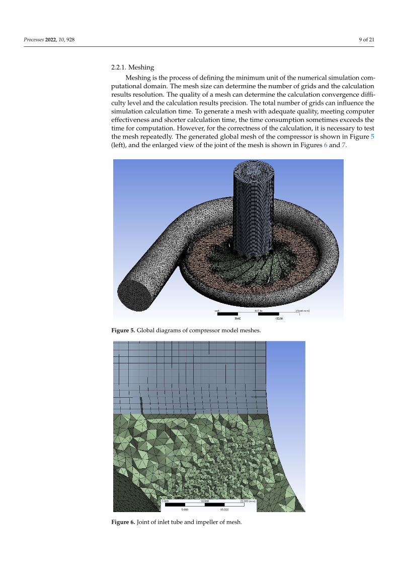
2.2.1. Meshing

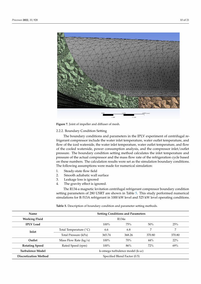
Meshing is the process of defining the minimum unit of the numerical simulation com-putational domain. The mesh size can determine the number of grids and the calculationresults resolution. The quality of a mesh can determine the calculation convergence diffi-culty level and the calculation results precision. The total number of grids can influence thesimulation calculation time. To generate a mesh with adequate quality, meeting computereffectiveness and shorter calculation time, the time consumption sometimes exceeds thetime for computation. However, for the correctness of the calculation, it is necessary to testthe mesh repeatedly. The generated global mesh of the compressor is shown in Figure 5(left), and the enlarged view of the joint of the mesh is shown in Figures 6 and 7.

Processes 2022, 10, x FOR PEER REVIEW 9 of 22

Figure 4. Flow field simulation analysis structure diagram.

2.2.1. Meshing Meshing is the process of defining the minimum unit of the numerical simulation com-

putational domain. The mesh size can determine the number of grids and the calculation results resolution. The quality of a mesh can determine the calculation convergence diffi-culty level and the calculation results precision. The total number of grids can influence the simulation calculation time. To generate a mesh with adequate quality, meeting computer effectiveness and shorter calculation time, the time consumption sometimes exceeds the time for computation. However, for the correctness of the calculation, it is necessary to test the mesh repeatedly. The generated global mesh of the compressor is shown in Figure 5 (left), and the enlarged view of the joint of the mesh is shown in Figures 6 and 7.

Figure 5. Global diagrams of compressor model meshes.

Processes 2022, 10, x FOR PEER REVIEW 10 of 22

Figure 5. Global diagrams of compressor model meshes.

Figure 6. Joint of inlet tube and impeller of mesh.

Figure 7. Joint of impeller and diffuser of mesh.

2.2.2. Boundary Condition Setting The boundary conditions and parameters in the IPLV experiment of centrifugal re-

frigerant compressor include the water inlet temperature, water outlet temperature, and flow of the iced waterside, the water inlet temperature, water outlet temperature, and flow

Figure 6. Joint of inlet tube and impeller of mesh.

Processes 2022, 10, 928 10 of 21

Processes 2022, 10, x FOR PEER REVIEW 10 of 22

Figure 5. Global diagrams of compressor model meshes.

Figure 6. Joint of inlet tube and impeller of mesh.

Figure 7. Joint of impeller and diffuser of mesh.

2.2.2. Boundary Condition Setting The boundary conditions and parameters in the IPLV experiment of centrifugal re-

frigerant compressor include the water inlet temperature, water outlet temperature, and flow of the iced waterside, the water inlet temperature, water outlet temperature, and flow

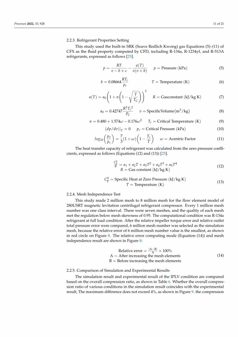
Figure 7. Joint of impeller and diffuser of mesh.

2.2.2. Boundary Condition Setting

The boundary conditions and parameters in the IPLV experiment of centrifugal re-frigerant compressor include the water inlet temperature, water outlet temperature, andflow of the iced waterside, the water inlet temperature, water outlet temperature, and flowof the cooled waterside, power consumption analysis, and the compressor inlet/outletpressure. The boundary condition setting method calculates the inlet temperature andpressure of the actual compressor and the mass flow rate of the refrigeration cycle basedon these numbers. The calculation results were set as the simulation boundary conditions.The following assumptions were made for numerical simulation:

1. Steady-state flow field2. Smooth adiabatic wall surface3. Leakage loss is ignored4. The gravity effect is ignored.

The R134-a magnetic levitation centrifugal refrigerant compressor boundary conditionsetting parameters of 280 USRT are shown in Table 5. This study performed numericalsimulations for R-513A refrigerant in 1000 kW level and 525 kW level operating conditions.

Table 5. Description of boundary condition and parameter setting methods.

Name Setting Conditions and Parameters

Working Fluid R134a

IPLV Load 100% 75% 50% 25%

InletTotal Temperature (◦C) 6.6 6.8 7 7

Total Pressure (kPa) 365.74 368.26 370.80 370.80

Outlet Mass Flow Rate (kg/s) 100% 70% 44% 22%

Rotating Speed Rated Speed (rpm) 100% 86% 72% 69%

Turbulence Model k-omega turbulence model (k-ω)

Discretization Method Specified Blend Factor (0.5)

Processes 2022, 10, 928 11 of 21

2.2.3. Refrigerant Properties Setting

This study used the built-in SRK (Soave Redlich Kwong) gas Equations (5)–(11) ofCFX as the fluid property computed by CFD, including R-134a, R-1234yf, and R-513Arefrigerants, expressed as follows [25].

p =RT

v− b + c− a(T)

v(v + b)p = Pressure (kPa) (5)

b = 0.08664RTc

pcT = Temperature (K) (6)

a(T) = a0

(1 + n

(1−

√TTC

))2

R = Gasconstant (kJ/kg K) (7)

a0 = 0.42747R2Tc

2

PCv = SpecificVolume

(m3/kg

)(8)

n = 0.480 + 1.574ω− 0.176ω2 Tc = Critical Temperature (K) (9)

(dp/dv)|T = 0 pc = Critical Pressure (kPa) (10)

log10

(pv

pc

)=

73(1 + ω)

(1− Tc

T

)ω = Acentric Factor (11)

The heat transfer capacity of refrigerant was calculated from the zero pressure coeffi-cients, expressed as follows (Equations (12) and (13)) [25].

C0p

R = a1 + a2T + a3T2 + a4T3 + a5T4

R = Gas constant (kJ/kg K)(12)

C0p = Specific Heat at Zero Pressure (kJ/kg K)

T = Temperature (K)(13)

2.2.4. Mesh Independence Test

This study made 2 million mesh to 8 million mesh for the flow element model of280USRT magnetic levitation centrifugal refrigerant compressor. Every 1 million meshnumber was one class interval. There were seven meshes, and the quality of each meshmet the regulation below mesh skewness of 0.95. The computational condition was R-134arefrigerant at full load condition. After the relative impeller torque error and relative outlettotal pressure error were compared, 6 million mesh number was selected as the simulationmesh, because the relative error of 6 million mesh number value is the smallest, as shownin red circle on Figure 8. The relative error computing mode (Equation (14)) and meshindependence result are shown in Figure 8:

Relative error = |A−B|A × 100%

A = After increasing the mesh elementsB = Before increasing the mesh elements

(14)

2.2.5. Comparison of Simulation and Experimental Results

The simulation result and experimental result of the IPLV condition are comparedbased on the overall compression ratio, as shown in Table 6. Whether the overall compres-sion ratio of various conditions in the simulation result coincides with the experimentalresult, The maximum difference does not exceed 4%, as shown in Figure 9. the compression

Processes 2022, 10, 928 12 of 21

ratio computing method and difference computing method (Equations (15) and (16)) areexpressed as follows:

Total Pressure Ratio =Outlet Total Pressure (kPa)Inlet Total Pressure (kPa)

(15)

Relative error = |A−B|B × 100%

A = Experimental total pressure ratioB = Simulated total pressure ratio

(16)

Processes 2022, 10, x FOR PEER REVIEW 12 of 22

2.2.4. Mesh Independence Test This study made 2 million mesh to 8 million mesh for the flow element model of

280USRT magnetic levitation centrifugal refrigerant compressor. Every 1 million mesh number was one class interval. There were seven meshes, and the quality of each mesh met the regulation below mesh skewness of 0.95. The computational condition was R-134a refrigerant at full load condition. After the relative impeller torque error and relative out-let total pressure error were compared, 6 million mesh number was selected as the simu-lation mesh, because the relative error of 6 million mesh number value is the smallest,as shown in red circle on Figure 8. The relative error computing mode (Equation (14)) and mesh independence result are shown in Figure 8: Relative error = |A − B|A × 100%

A = After increasing the mesh elements B = Before increasing the mesh elements

(14)

Figure 8. Schematic diagram of mesh independence test.

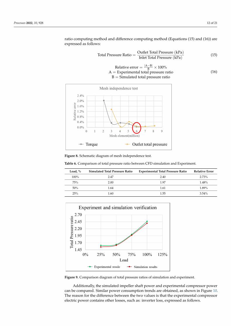
2.2.5. Comparison of Simulation and Experimental Results The simulation result and experimental result of the IPLV condition are compared

based on the overall compression ratio,as shown in Table 6. Whether the overall compres-sion ratio of various conditions in the simulation result coincides with the experimental result, The maximum difference does not exceed 4%, as shown in Figure 9. the compres-sion ratio computing method and difference computing method (Equations (15) and (16)) are expressed as follows: Total Pressure Ratio = Outlet Total Pressure kPaInlet Total Pressure kPa (15)

Figure 8. Schematic diagram of mesh independence test.

Table 6. Comparison of total pressure ratio between CFD simulation and Experiment.

Load, % Simulated Total Pressure Ratio Experimental Total Pressure Ratio Relative Error

100% 2.47 2.40 2.73%

75% 2.00 1.97 1.48%

50% 1.64 1.61 1.89%

25% 1.60 1.55 3.54%

Processes 2022, 10, x FOR PEER REVIEW 12 of 22

2.2.4. Mesh Independence Test This study made 2 million mesh to 8 million mesh for the flow element model of

280USRT magnetic levitation centrifugal refrigerant compressor. Every 1 million mesh number was one class interval. There were seven meshes, and the quality of each mesh met the regulation below mesh skewness of 0.95. The computational condition was R-134a refrigerant at full load condition. After the relative impeller torque error and relative out-let total pressure error were compared, 6 million mesh number was selected as the simu-lation mesh, because the relative error of 6 million mesh number value is the smallest,as shown in red circle on Figure 8. The relative error computing mode (Equation (14)) and mesh independence result are shown in Figure 8: Relative error = |A − B|A × 100%

A = After increasing the mesh elements B = Before increasing the mesh elements

(14)

Figure 8. Schematic diagram of mesh independence test.

2.2.5. Comparison of Simulation and Experimental Results The simulation result and experimental result of the IPLV condition are compared

based on the overall compression ratio,as shown in Table 6. Whether the overall compres-sion ratio of various conditions in the simulation result coincides with the experimental result, The maximum difference does not exceed 4%, as shown in Figure 9. the compres-sion ratio computing method and difference computing method (Equations (15) and (16)) are expressed as follows: Total Pressure Ratio = Outlet Total Pressure kPaInlet Total Pressure kPa (15)

Figure 9. Comparison diagram of total pressure ratios of simulation and experiment.

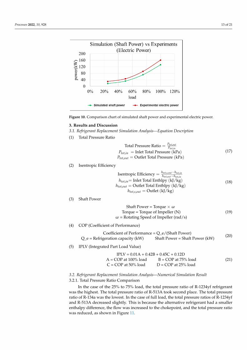
Additionally, the simulated impeller shaft power and experimental compressor powercan be compared. Similar power consumption trends are obtained, as shown in Figure 10.The reason for the difference between the two values is that the experimental compressorelectric power contains other losses, such as: inverter loss, expressed as follows.

Processes 2022, 10, 928 13 of 21

Processes 2022, 10, x FOR PEER REVIEW 13 of 22

Figure 9. Comparison diagram of total pressure ratios of simulation and experiment.

Relative error = |A − B|B × 100%

A = Experimental total pressure ratio B = Simulated total pressure ratio

(16)

Table 6. Comparison of total pressure ratio between CFD simulation and Experiment.

Load, % Simulated Total Pressure Ratio Experimental Total Pressure Ratio Relative Error 100% 2.47 2.40 2.73% 75% 2.00 1.97 1.48% 50% 1.64 1.61 1.89% 25% 1.60 1.55 3.54%

Additionally, the simulated impeller shaft power and experimental compressor power can be compared. Similar power consumption trends are obtained, as shown in Figure 10. The reason for the difference between the two values is that the experimental compressor electric power contains other losses, such as: inverter loss, expressed as fol-lows.

Figure 10. Comparison chart of simulated shaft power and experimental electric power.

3. Results and Discussion 3.1. Refrigerant Replacement Simulation Analysis—Equation Description (1) Total Pressure Ratio Total Pressure Ratio = 𝑃 ,𝑃 , 𝑃 , = Inlet Total Pressure(kPa) 𝑃 , = Outlet Total Pressure(kPa)

(17)

(2) Isentropic Efficiency Isentropic Efficiency = , , ,, , ℎ , = Inlet Total Enthlpy(kJ/kg) ℎ , = Outlet Total Enthlpy(kJ/kg) ℎ , , = Outlet (kJ/kg) (18)

(3) Shaft Power

Shaft Power = Torque × ω Torque = Torque of Impeller(N) ω = Rotating Speed of Impeller (rad/s) (19)

(4) COP (Coefficient of Performance)

Figure 10. Comparison chart of simulated shaft power and experimental electric power.

3. Results and Discussion3.1. Refrigerant Replacement Simulation Analysis—Equation Description

(1) Total Pressure Ratio

Total Pressure Ratio =Ptot,outPtot,in

Ptot,in = Inlet Total Pressure (kPa)Ptot,out = Outlet Total Pressure (kPa)

(17)

(2) Isentropic Efficiency

Isentropic Efficiency =htot,s,out−htot,inhtot,out−htot,in

htot,in= Inlet Total Enthlpy (kJ/kg)htot,out = Outlet Total Enthlpy (kJ/kg)

htot,s,out = Outlet (kJ/kg)

(18)

(3) Shaft Power

Shaft Power = Torque × ω

Torque = Torque of Impeller (N)ω = Rotating Speed of Impeller (rad/s)

(19)

(4) COP (Coefficient of Performance)

Coefficient of Performance = Q_e/(Shaft Power)Q_e = Refrigeration capacity (kW) Shaft Power = Shaft Power (kW)

(20)

(5) IPLV (Integrated Part Load Value)

IPLV = 0.01A + 0.42B + 0.45C + 0.12DA = COP at 100% load B = COP at 75% loadC = COP at 50% load D = COP at 25% load

(21)

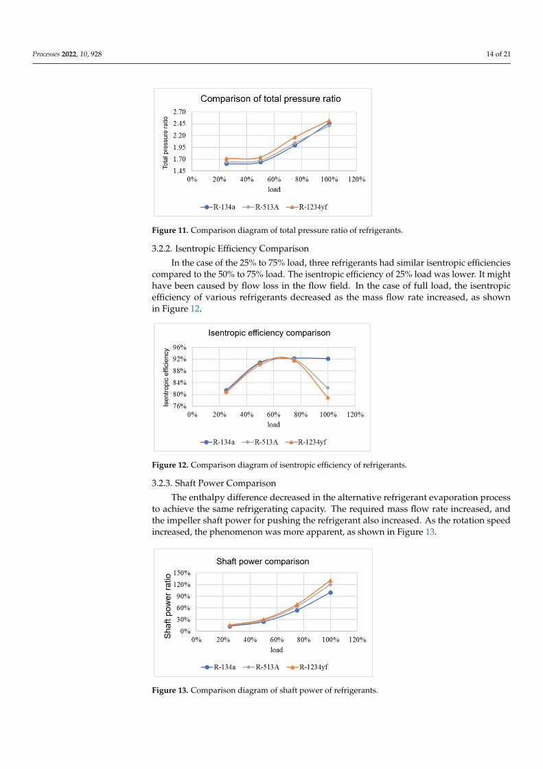
3.2. Refrigerant Replacement Simulation Analysis—Numerical Simulation Result3.2.1. Total Pressure Ratio Comparison

In the case of the 25% to 75% load, the total pressure ratio of R-1234yf refrigerantwas the highest. The total pressure ratio of R-513A took second place. The total pressureratio of R-134a was the lowest. In the case of full load, the total pressure ratios of R-1234yfand R-513A decreased slightly. This is because the alternative refrigerant had a smallerenthalpy difference, the flow was increased to the chokepoint, and the total pressure ratiowas reduced, as shown in Figure 11.

Processes 2022, 10, 928 14 of 21

Processes 2022, 10, x FOR PEER REVIEW 14 of 22

Coefficient of Performance = Q_e/(Shaft Power) Q_e= Refrigeration capacity (kW) Shaft Power = Shaft Power(kW) (20)

(5) IPLV (Integrated Part Load Value)

IPLV = 0.01A + 0.42B + 0.45C + 0.12D A = COP at 100% load B = COP at 75% load C = COP at 50% load D = COP at 25% load

(21)

3.2. Refrigerant Replacement Simulation Analysis—Numerical Simulation Result 3.2.1. Total Pressure Ratio Comparison

In the case of the 25% to 75% load, the total pressure ratio of R-1234yf refrigerant was the highest. The total pressure ratio of R-513A took second place. The total pressure ratio of R-134a was the lowest. In the case of full load, the total pressure ratios of R-1234yf and R-513A decreased slightly. This is because the alternative refrigerant had a smaller en-thalpy difference, the flow was increased to the chokepoint, and the total pressure ratio was reduced, as shown in Figure 11.

Figure 11. Comparison diagram of total pressure ratio of refrigerants.

3.2.2. Isentropic Efficiency Comparison In the case of the 25% to 75% load, three refrigerants had similar isentropic efficien-

cies compared to the 50% to 75% load. The isentropic efficiency of 25% load was lower. It might have been caused by flow loss in the flow field. In the case of full load, the isentropic efficiency of various refrigerants decreased as the mass flow rate increased, as shown in Figure 12.

Figure 12. Comparison diagram of isentropic efficiency of refrigerants.

3.2.3. Shaft Power Comparison

Figure 11. Comparison diagram of total pressure ratio of refrigerants.

3.2.2. Isentropic Efficiency Comparison

In the case of the 25% to 75% load, three refrigerants had similar isentropic efficienciescompared to the 50% to 75% load. The isentropic efficiency of 25% load was lower. It mighthave been caused by flow loss in the flow field. In the case of full load, the isentropicefficiency of various refrigerants decreased as the mass flow rate increased, as shownin Figure 12.

Processes 2022, 10, x FOR PEER REVIEW 14 of 22

Coefficient of Performance = Q_e/(Shaft Power) Q_e= Refrigeration capacity (kW) Shaft Power = Shaft Power(kW) (20)

(5) IPLV (Integrated Part Load Value)

IPLV = 0.01A + 0.42B + 0.45C + 0.12D A = COP at 100% load B = COP at 75% load C = COP at 50% load D = COP at 25% load

(21)

3.2. Refrigerant Replacement Simulation Analysis—Numerical Simulation Result 3.2.1. Total Pressure Ratio Comparison

In the case of the 25% to 75% load, the total pressure ratio of R-1234yf refrigerant was the highest. The total pressure ratio of R-513A took second place. The total pressure ratio of R-134a was the lowest. In the case of full load, the total pressure ratios of R-1234yf and R-513A decreased slightly. This is because the alternative refrigerant had a smaller en-thalpy difference, the flow was increased to the chokepoint, and the total pressure ratio was reduced, as shown in Figure 11.

Figure 11. Comparison diagram of total pressure ratio of refrigerants.

3.2.2. Isentropic Efficiency Comparison In the case of the 25% to 75% load, three refrigerants had similar isentropic efficien-

cies compared to the 50% to 75% load. The isentropic efficiency of 25% load was lower. It might have been caused by flow loss in the flow field. In the case of full load, the isentropic efficiency of various refrigerants decreased as the mass flow rate increased, as shown in Figure 12.

Figure 12. Comparison diagram of isentropic efficiency of refrigerants.

3.2.3. Shaft Power Comparison

Figure 12. Comparison diagram of isentropic efficiency of refrigerants.

3.2.3. Shaft Power Comparison

The enthalpy difference decreased in the alternative refrigerant evaporation processto achieve the same refrigerating capacity. The required mass flow rate increased, andthe impeller shaft power for pushing the refrigerant also increased. As the rotation speedincreased, the phenomenon was more apparent, as shown in Figure 13.

Processes 2022, 10, x FOR PEER REVIEW 15 of 22

The enthalpy difference decreased in the alternative refrigerant evaporation process to achieve the same refrigerating capacity. The required mass flow rate increased, and the impeller shaft power for pushing the refrigerant also increased. As the rotation speed in-creased, the phenomenon was more apparent, as shown in Figure 13.

Figure 13. Comparison diagram of shaft power of refrigerants.

3.2.4. COP Comparison The R-134a refrigerant had the highest COP in various conditions. The R-1234yf re-

frigerant had the lowest COP, and the R-513A was intermediate among the other two re-frigerants, as shown in Figure 14.

Figure 14. Comparison diagram of COP of refrigerants.

3.2.5. IPLV Comparison After IPLV weighted calculation, compared to singly comparing full load COP, the

IPLV values of various refrigerants are closer, as shown in Figure 15.

Figure 15. Comparison diagram of full load COP and IPLV of refrigerants.

3.3. Refrigerant Replacement Simulation Analysis—Flow Field Simulation Result

Figure 13. Comparison diagram of shaft power of refrigerants.

Processes 2022, 10, 928 15 of 21

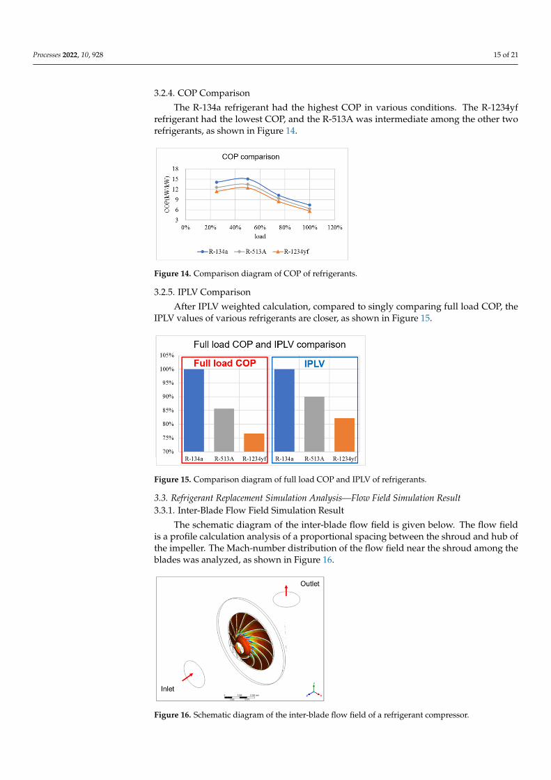
3.2.4. COP Comparison

The R-134a refrigerant had the highest COP in various conditions. The R-1234yfrefrigerant had the lowest COP, and the R-513A was intermediate among the other tworefrigerants, as shown in Figure 14.

Processes 2022, 10, x FOR PEER REVIEW 15 of 22

The enthalpy difference decreased in the alternative refrigerant evaporation process to achieve the same refrigerating capacity. The required mass flow rate increased, and the impeller shaft power for pushing the refrigerant also increased. As the rotation speed in-creased, the phenomenon was more apparent, as shown in Figure 13.

Figure 13. Comparison diagram of shaft power of refrigerants.

3.2.4. COP Comparison The R-134a refrigerant had the highest COP in various conditions. The R-1234yf re-

frigerant had the lowest COP, and the R-513A was intermediate among the other two re-frigerants, as shown in Figure 14.

Figure 14. Comparison diagram of COP of refrigerants.

3.2.5. IPLV Comparison After IPLV weighted calculation, compared to singly comparing full load COP, the

IPLV values of various refrigerants are closer, as shown in Figure 15.

Figure 15. Comparison diagram of full load COP and IPLV of refrigerants.

3.3. Refrigerant Replacement Simulation Analysis—Flow Field Simulation Result

Figure 14. Comparison diagram of COP of refrigerants.

3.2.5. IPLV Comparison

After IPLV weighted calculation, compared to singly comparing full load COP, theIPLV values of various refrigerants are closer, as shown in Figure 15.

Processes 2022, 10, x FOR PEER REVIEW 15 of 22

The enthalpy difference decreased in the alternative refrigerant evaporation process to achieve the same refrigerating capacity. The required mass flow rate increased, and the impeller shaft power for pushing the refrigerant also increased. As the rotation speed in-creased, the phenomenon was more apparent, as shown in Figure 13.

Figure 13. Comparison diagram of shaft power of refrigerants.

3.2.4. COP Comparison The R-134a refrigerant had the highest COP in various conditions. The R-1234yf re-

frigerant had the lowest COP, and the R-513A was intermediate among the other two re-frigerants, as shown in Figure 14.

Figure 14. Comparison diagram of COP of refrigerants.

3.2.5. IPLV Comparison After IPLV weighted calculation, compared to singly comparing full load COP, the

IPLV values of various refrigerants are closer, as shown in Figure 15.

Figure 15. Comparison diagram of full load COP and IPLV of refrigerants.

3.3. Refrigerant Replacement Simulation Analysis—Flow Field Simulation Result

Figure 15. Comparison diagram of full load COP and IPLV of refrigerants.

3.3. Refrigerant Replacement Simulation Analysis—Flow Field Simulation Result3.3.1. Inter-Blade Flow Field Simulation Result

The schematic diagram of the inter-blade flow field is given below. The flow fieldis a profile calculation analysis of a proportional spacing between the shroud and hub ofthe impeller. The Mach-number distribution of the flow field near the shroud among theblades was analyzed, as shown in Figure 16.

Processes 2022, 10, x FOR PEER REVIEW 16 of 22

3.3.1. Inter-Blade Flow Field Simulation Result The schematic diagram of the inter-blade flow field is given below. The flow field is

a profile calculation analysis of a proportional spacing between the shroud and hub of the impeller. The Mach-number distribution of the flow field near the shroud among the blades was analyzed, as shown in Figure 16.

Figure 16. Schematic diagram of the inter-blade flow field of a refrigerant compressor.

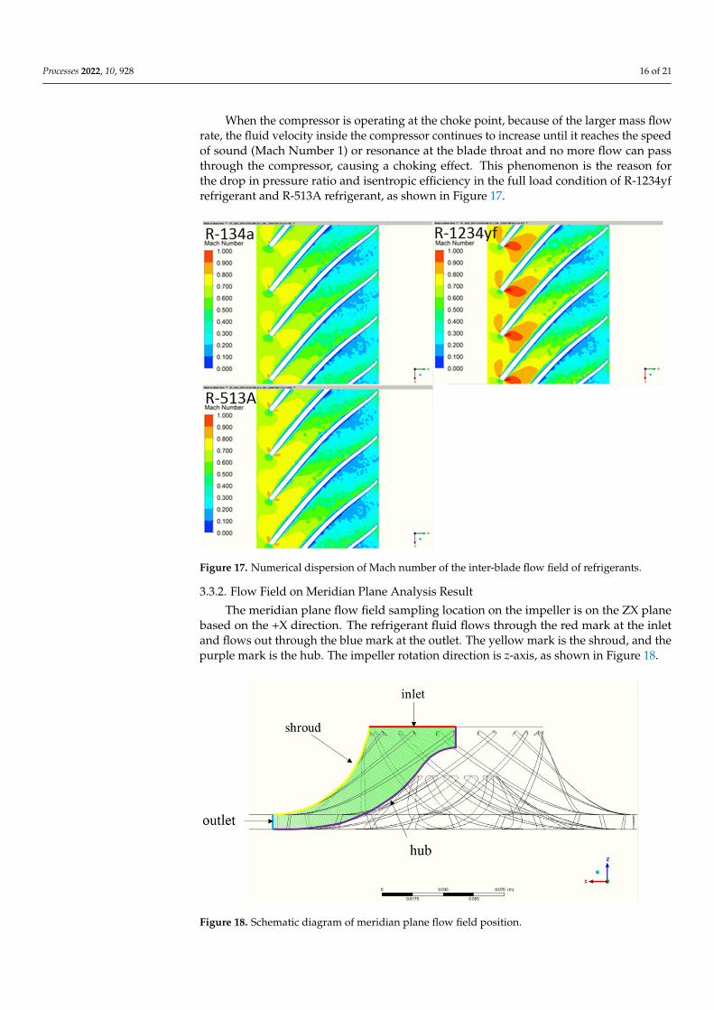
When the compressor is operating at the choke point, because of the larger mass flow rate, the fluid velocity inside the compressor continues to increase until it reaches the speed of sound (Mach Number 1) or resonance at the blade throat and no more flow can pass through the compressor, causing a choking effect. This phenomenon is the reason for the drop in pressure ratio and isentropic efficiency in the full load condition of R-1234yf refrigerant and R-513A refrigerant, as shown in Figure 17.

Figure 17. Numerical dispersion of Mach number of the inter-blade flow field of refrigerants.

3.3.2. Flow Field on Meridian Plane Analysis Result The meridian plane flow field sampling location on the impeller is on the ZX plane

based on the +X direction. The refrigerant fluid flows through the red mark at the inlet

Figure 16. Schematic diagram of the inter-blade flow field of a refrigerant compressor.

Processes 2022, 10, 928 16 of 21

When the compressor is operating at the choke point, because of the larger mass flowrate, the fluid velocity inside the compressor continues to increase until it reaches the speedof sound (Mach Number 1) or resonance at the blade throat and no more flow can passthrough the compressor, causing a choking effect. This phenomenon is the reason forthe drop in pressure ratio and isentropic efficiency in the full load condition of R-1234yfrefrigerant and R-513A refrigerant, as shown in Figure 17.

Processes 2022, 10, x FOR PEER REVIEW 16 of 22

3.3.1. Inter-Blade Flow Field Simulation Result The schematic diagram of the inter-blade flow field is given below. The flow field is

a profile calculation analysis of a proportional spacing between the shroud and hub of the impeller. The Mach-number distribution of the flow field near the shroud among the blades was analyzed, as shown in Figure 16.

Figure 16. Schematic diagram of the inter-blade flow field of a refrigerant compressor.

When the compressor is operating at the choke point, because of the larger mass flow rate, the fluid velocity inside the compressor continues to increase until it reaches the speed of sound (Mach Number 1) or resonance at the blade throat and no more flow can pass through the compressor, causing a choking effect. This phenomenon is the reason for the drop in pressure ratio and isentropic efficiency in the full load condition of R-1234yf refrigerant and R-513A refrigerant, as shown in Figure 17.

Figure 17. Numerical dispersion of Mach number of the inter-blade flow field of refrigerants.

3.3.2. Flow Field on Meridian Plane Analysis Result The meridian plane flow field sampling location on the impeller is on the ZX plane

based on the +X direction. The refrigerant fluid flows through the red mark at the inlet

Figure 17. Numerical dispersion of Mach number of the inter-blade flow field of refrigerants.

3.3.2. Flow Field on Meridian Plane Analysis Result

The meridian plane flow field sampling location on the impeller is on the ZX planebased on the +X direction. The refrigerant fluid flows through the red mark at the inletand flows out through the blue mark at the outlet. The yellow mark is the shroud, and thepurple mark is the hub. The impeller rotation direction is z-axis, as shown in Figure 18.

Processes 2022, 10, x FOR PEER REVIEW 17 of 22

and flows out through the blue mark at the outlet. The yellow mark is the shroud, and the purple mark is the hub. The impeller rotation direction is -z-axis, as shown in Figure 18.

Figure 18. Schematic diagram of meridian plane flow field position.

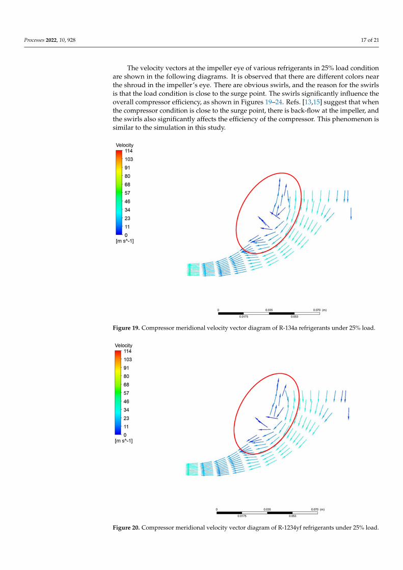
The velocity vectors at the impeller eye of various refrigerants in 25% load condition are shown in the following diagrams. It is observed that there are different colors near the shroud in the impeller’s eye. There are obvious swirls, and the reason for the swirls is that the load condition is close to the surge point. The swirls significantly influence the overall compressor efficiency, as shown in Figures 19–24. Refs. [13,15] suggest that when the com-pressor condition is close to the surge point, there is back-flow at the impeller, and the swirls also significantly affects the efficiency of the compressor. This phenomenon is sim-ilar to the simulation in this study.

Figure 19. Compressor meridional velocity vector diagram of R-134a refrigerants under 25% load.

Figure 18. Schematic diagram of meridian plane flow field position.

Processes 2022, 10, 928 17 of 21

The velocity vectors at the impeller eye of various refrigerants in 25% load conditionare shown in the following diagrams. It is observed that there are different colors nearthe shroud in the impeller’s eye. There are obvious swirls, and the reason for the swirlsis that the load condition is close to the surge point. The swirls significantly influence theoverall compressor efficiency, as shown in Figures 19–24. Refs. [13,15] suggest that whenthe compressor condition is close to the surge point, there is back-flow at the impeller, andthe swirls also significantly affects the efficiency of the compressor. This phenomenon issimilar to the simulation in this study.

Processes 2022, 10, x FOR PEER REVIEW 17 of 22

and flows out through the blue mark at the outlet. The yellow mark is the shroud, and the purple mark is the hub. The impeller rotation direction is -z-axis, as shown in Figure 18.

Figure 18. Schematic diagram of meridian plane flow field position.

The velocity vectors at the impeller eye of various refrigerants in 25% load condition are shown in the following diagrams. It is observed that there are different colors near the shroud in the impeller’s eye. There are obvious swirls, and the reason for the swirls is that the load condition is close to the surge point. The swirls significantly influence the overall compressor efficiency, as shown in Figures 19–24. Refs. [13,15] suggest that when the com-pressor condition is close to the surge point, there is back-flow at the impeller, and the swirls also significantly affects the efficiency of the compressor. This phenomenon is sim-ilar to the simulation in this study.

Figure 19. Compressor meridional velocity vector diagram of R-134a refrigerants under 25% load. Figure 19. Compressor meridional velocity vector diagram of R-134a refrigerants under 25% load.

Processes 2022, 10, x FOR PEER REVIEW 18 of 22

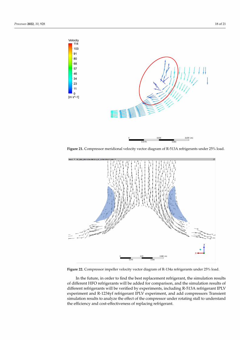
Figure 20. Compressor meridional velocity vector diagram of R-1234yf refrigerants under 25% load.

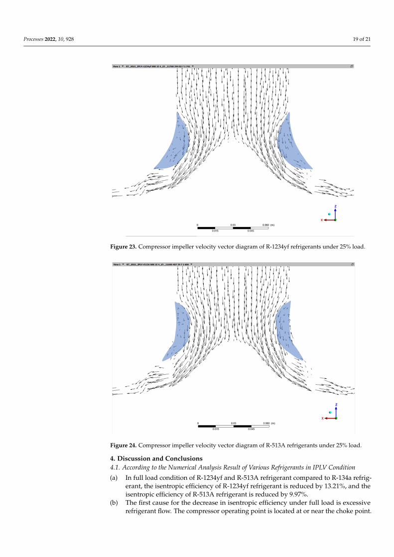
Figure 21. Compressor meridional velocity vector diagram of R-513A refrigerants under 25% load.

Figure 20. Compressor meridional velocity vector diagram of R-1234yf refrigerants under 25% load.

Processes 2022, 10, 928 18 of 21

Processes 2022, 10, x FOR PEER REVIEW 18 of 22

Figure 20. Compressor meridional velocity vector diagram of R-1234yf refrigerants under 25% load.

Figure 21. Compressor meridional velocity vector diagram of R-513A refrigerants under 25% load. Figure 21. Compressor meridional velocity vector diagram of R-513A refrigerants under 25% load.

Processes 2022, 10, x FOR PEER REVIEW 19 of 22

Figure 22. Compressor impeller velocity vector diagram of R-134a refrigerants under 25% load.

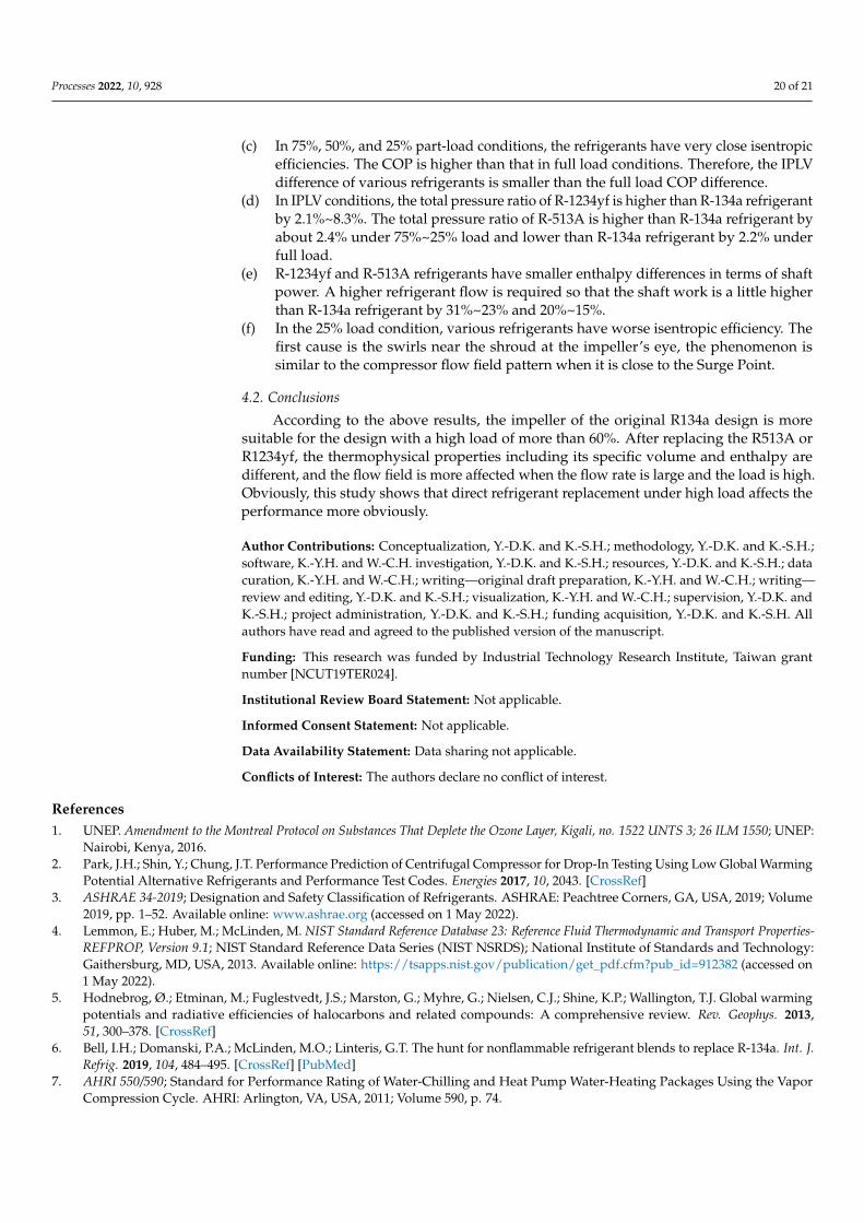
Figure 23. Compressor impeller velocity vector diagram of R-1234yf refrigerants under 25% load.

Figure 22. Compressor impeller velocity vector diagram of R-134a refrigerants under 25% load.

In the future, in order to find the best replacement refrigerant, the simulation resultsof different HFO refrigerants will be added for comparison, and the simulation results ofdifferent refrigerants will be verified by experiments, including R-513A refrigerant IPLVexperiment and R-1234yf refrigerant IPLV experiment, and add compressors Transientsimulation results to analyze the effect of the compressor under rotating stall to understandthe efficiency and cost-effectiveness of replacing refrigerant.

Processes 2022, 10, 928 19 of 21

Processes 2022, 10, x FOR PEER REVIEW 19 of 22

Figure 22. Compressor impeller velocity vector diagram of R-134a refrigerants under 25% load.

Figure 23. Compressor impeller velocity vector diagram of R-1234yf refrigerants under 25% load. Figure 23. Compressor impeller velocity vector diagram of R-1234yf refrigerants under 25% load.

Processes 2022, 10, x FOR PEER REVIEW 20 of 22

Figure 24. Compressor impeller velocity vector diagram of R-513A refrigerants under 25% load.

In the future, in order to find the best replacement refrigerant, the simulation results of different HFO refrigerants will be added for comparison, and the simulation results of different refrigerants will be verified by experiments, including R-513A refrigerant IPLV experiment and R-1234yf refrigerant IPLV experiment, and add compressors Transient simulation results to analyze the effect of the compressor under rotating stall to under-stand the efficiency and cost-effectiveness of replacing refrigerant.

4. Discussion and Conclusions 4.1. According to the Numerical Analysis Result of Various Refrigerants in IPLV Condition (a) In full load condition of R-1234yf and R-513A refrigerant compared to R-134a refrig-

erant, the isentropic efficiency of R-1234yf refrigerant is reduced by 13.21%, and the isentropic efficiency of R-513A refrigerant is reduced by 9.97%.

(b) The first cause for the decrease in isentropic efficiency under full load is excessive refrigerant flow. The compressor operating point is located at or near the choke point.

(c) In 75%, 50%, and 25% part-load conditions, the refrigerants have very close isentropic efficiencies. The COP is higher than that in full load conditions. Therefore, the IPLV difference of various refrigerants is smaller than the full load COP difference.

(d) In IPLV conditions, the total pressure ratio of R-1234yf is higher than R-134a refrig-erant by 2.1%~8.3%. The total pressure ratio of R-513A is higher than R-134a refrig-erant by about 2.4% under 75%~25% load and lower than R-134a refrigerant by 2.2% under full load.

(e) R-1234yf and R-513A refrigerants have smaller enthalpy differences in terms of shaft power. A higher refrigerant flow is required so that the shaft work is a little higher than R-134a refrigerant by 31%~23% and 20%~15%.

(f) In the 25% load condition, various refrigerants have worse isentropic efficiency. The first cause is the swirls near the shroud at the impeller’s eye, the phenomenon is sim-ilar to the compressor flow field pattern when it is close to the Surge Point.

4.2. Conclusions According to the above results, the impeller of the original R134a design is more suit-

able for the design with a high load of more than 60%. After replacing the R513A or R1234yf, the thermophysical properties including its specific volume and enthalpy are different, and the flow field is more affected when the flow rate is large and the load is

Figure 24. Compressor impeller velocity vector diagram of R-513A refrigerants under 25% load.

4. Discussion and Conclusions4.1. According to the Numerical Analysis Result of Various Refrigerants in IPLV Condition

(a) In full load condition of R-1234yf and R-513A refrigerant compared to R-134a refrig-erant, the isentropic efficiency of R-1234yf refrigerant is reduced by 13.21%, and theisentropic efficiency of R-513A refrigerant is reduced by 9.97%.

(b) The first cause for the decrease in isentropic efficiency under full load is excessiverefrigerant flow. The compressor operating point is located at or near the choke point.

Processes 2022, 10, 928 20 of 21

(c) In 75%, 50%, and 25% part-load conditions, the refrigerants have very close isentropicefficiencies. The COP is higher than that in full load conditions. Therefore, the IPLVdifference of various refrigerants is smaller than the full load COP difference.

(d) In IPLV conditions, the total pressure ratio of R-1234yf is higher than R-134a refrigerantby 2.1%~8.3%. The total pressure ratio of R-513A is higher than R-134a refrigerant byabout 2.4% under 75%~25% load and lower than R-134a refrigerant by 2.2% underfull load.

(e) R-1234yf and R-513A refrigerants have smaller enthalpy differences in terms of shaftpower. A higher refrigerant flow is required so that the shaft work is a little higherthan R-134a refrigerant by 31%~23% and 20%~15%.

(f) In the 25% load condition, various refrigerants have worse isentropic efficiency. Thefirst cause is the swirls near the shroud at the impeller’s eye, the phenomenon issimilar to the compressor flow field pattern when it is close to the Surge Point.

4.2. Conclusions

According to the above results, the impeller of the original R134a design is moresuitable for the design with a high load of more than 60%. After replacing the R513A orR1234yf, the thermophysical properties including its specific volume and enthalpy aredifferent, and the flow field is more affected when the flow rate is large and the load is high.Obviously, this study shows that direct refrigerant replacement under high load affects theperformance more obviously.

Author Contributions: Conceptualization, Y.-D.K. and K.-S.H.; methodology, Y.-D.K. and K.-S.H.;software, K.-Y.H. and W.-C.H. investigation, Y.-D.K. and K.-S.H.; resources, Y.-D.K. and K.-S.H.; datacuration, K.-Y.H. and W.-C.H.; writing—original draft preparation, K.-Y.H. and W.-C.H.; writing—review and editing, Y.-D.K. and K.-S.H.; visualization, K.-Y.H. and W.-C.H.; supervision, Y.-D.K. andK.-S.H.; project administration, Y.-D.K. and K.-S.H.; funding acquisition, Y.-D.K. and K.-S.H. Allauthors have read and agreed to the published version of the manuscript.

Funding: This research was funded by Industrial Technology Research Institute, Taiwan grantnumber [NCUT19TER024].

Institutional Review Board Statement: Not applicable.

Informed Consent Statement: Not applicable.

Data Availability Statement: Data sharing not applicable.

Conflicts of Interest: The authors declare no conflict of interest.

References1. UNEP. Amendment to the Montreal Protocol on Substances That Deplete the Ozone Layer, Kigali, no. 1522 UNTS 3; 26 ILM 1550; UNEP:

Nairobi, Kenya, 2016.2. Park, J.H.; Shin, Y.; Chung, J.T. Performance Prediction of Centrifugal Compressor for Drop-In Testing Using Low Global Warming

Potential Alternative Refrigerants and Performance Test Codes. Energies 2017, 10, 2043. [CrossRef]3. ASHRAE 34-2019; Designation and Safety Classification of Refrigerants. ASHRAE: Peachtree Corners, GA, USA, 2019; Volume

2019, pp. 1–52. Available online: www.ashrae.org (accessed on 1 May 2022).4. Lemmon, E.; Huber, M.; McLinden, M. NIST Standard Reference Database 23: Reference Fluid Thermodynamic and Transport Properties-

REFPROP, Version 9.1; NIST Standard Reference Data Series (NIST NSRDS); National Institute of Standards and Technology:Gaithersburg, MD, USA, 2013. Available online: https://tsapps.nist.gov/publication/get_pdf.cfm?pub_id=912382 (accessed on1 May 2022).

5. Hodnebrog, Ø.; Etminan, M.; Fuglestvedt, J.S.; Marston, G.; Myhre, G.; Nielsen, C.J.; Shine, K.P.; Wallington, T.J. Global warmingpotentials and radiative efficiencies of halocarbons and related compounds: A comprehensive review. Rev. Geophys. 2013,51, 300–378. [CrossRef]

6. Bell, I.H.; Domanski, P.A.; McLinden, M.O.; Linteris, G.T. The hunt for nonflammable refrigerant blends to replace R-134a. Int. J.Refrig. 2019, 104, 484–495. [CrossRef] [PubMed]

7. AHRI 550/590; Standard for Performance Rating of Water-Chilling and Heat Pump Water-Heating Packages Using the VaporCompression Cycle. AHRI: Arlington, VA, USA, 2011; Volume 590, p. 74.

Processes 2022, 10, 928 21 of 21

8. Ghenaiet, A.; Khalfallah, S. Assessment of some stall-onset criteria for centrifugal compressors. Aerosp. Sci. Technol. 2019,88, 193–207. [CrossRef]

9. Velásquez, E.I.G. Determination of a suitable set of loss models for centrifugal compressor performance prediction. Chin. J.Aeronaut. 2017, 30, 1644–1650. [CrossRef]

10. Zhang, C.; Dong, X.; Liu, X.; Sun, Z.; Wu, S.; Gao, Q.; Tan, C. A method to select loss correlations for centrifugal compressorperformance prediction. Aerosp. Sci. Technol. 2019, 93, 1–15. [CrossRef]

11. Zhao, D.; Hua, Z.; Dou, M.; Huangfu, Y. Control oriented modeling and analysis of centrifugal compressor working characteristicat variable altitude. Aerosp. Sci. Technol. 2018, 72, 174–182. [CrossRef]

12. Kim, C.; Son, C. Comparative Study on Steady and Unsteady Flow in a Centrifugal Compressor Stage. Int. J. Aerosp. Eng. 2019,2019, 1–12. [CrossRef]

13. Zhang, H.; Yang, C.; Shi, X.; Yang, C.; Chen, J. Two stall stages in a centrifugal compressor with a vaneless diffuser. Aerosp. Sci.Technol. 2021, 110, 106496. [CrossRef]

14. Tiwari, R.; Bordoloi, D.; Dewangan, A. Blockage and cavitation detection in centrifugal pumps from dynamic pressure signalusing deep learning algorithm. Meas. J. Int. Meas. Confed. 2021, 173, 108676. [CrossRef]

15. Semlitsch, B.; Mihaescu, M. Flow phenomena leading to surge in a centrifugal compressor. Energy 2016, 103, 572–587. [CrossRef]16. Galindo, J.; Gil, A.; Navarro, R.; Tarí, D. Analysis of the impact of the geometry on the performance of an automotive centrifugal

compressor using CFD simulations. Appl. Therm. Eng. 2019, 148, 1324–1333. [CrossRef]17. Sun, J.; Li, W.; Cui, B. Energy and exergy analyses of R513a as a R134a drop-in replacement in a vapor compression refrigeration

system. Int. J. Refrig. 2020, 112, 348–356. [CrossRef]18. Yang, M.; Zhang, H.; Meng, Z.; Qin, Y. Experimental study on R1234yf/R134a mixture (R513A) as R134a replacement in a

domestic refrigerator. Appl. Therm. Eng. 2019, 146, 540–547. [CrossRef]19. Mota-Babiloni, A.; Belman-Flores, J.M.; Makhnatch, P.; Navarro-Esbrí, J.; Barroso-Maldonado, J.M. Experimental exergy analysis

of R513A to replace R134a in a small capacity refrigeration system. Energy 2018, 162, 99–110. [CrossRef]20. Velasco, F.; Illán-Gómez, F.; García-Cascales, J. Energy efficiency evaluation of the use of R513A as a drop-in replacement for

R134a in a water chiller with a minichannel condenser for air-conditioning applications. Appl. Therm. Eng. 2021, 182, 115915.[CrossRef]

21. Al-Sayyab, A.K.S.; Mota-Babiloni, A.; Navarro-Esbrí, J. Novel compound waste heat-solar driven ejector-compression heat pumpfor simultaneous cooling and heating using environmentally friendly refrigerants. Energy Convers. Manag. 2021, 228, 113703.[CrossRef]

22. Pérez-García, V.; Mota-Babiloni, A.; Navarro-Esbrí, J. Influence of operational modes of the internal heat exchanger in anexperimental installation using R-450A and R-513A as replacement alternatives for R-134a. Energy 2019, 189, 116348. [CrossRef]

23. Wang, C.-C. An overview for the heat transfer performance of HFO-1234yf. Renew. Sustain. Energy Rev. 2013, 19, 444–453.[CrossRef]

24. Jankovic, Z.; Atienza, J.S.; Suárez, J.A.M. Thermodynamic and heat transfer analyses for R1234yf and R1234ze(E) as drop-inreplacements for R134a in a small power refrigerating system. Appl. Therm. Eng. 2015, 80, 42–54. [CrossRef]

25. ANSYS. ANSYS CFX-Solver Theory Guide. Release 14.0; ANSYS: Canonsburg, PA, USA, 2011; Volume 15317, pp. 724–746. Availableonline: http://www1.ansys.com/customer/content/documentation/140/cfx_thry.pdf (accessed on 1 May 2022).

26. Acharya, R. Investigation of Differences in Ansys Solvers CFX and Fluent; KTH Royal Institute of Technology: Stockholm, Sweden, 2016.