CGEH Working Paper Series The Changing Shape of Global Inequality 1820-2000: Exploring a new dataset Jan Luiten van Zanden, Utrecht University Joerg Baten, University of Tübingen Peter Földvari, University of Debrecen Bas van Leeuwen, Utrecht University January 2011 Working paper no. 1 http://www.cgeh.nl/working-paper-series/ © 2011 by Authors. All rights reserved. Short sections of text, not to exceed two paragraphs, may be quoted without explicit permission provided that full credit, including © notice, is given to the source.

Welcome message from author
This document is posted to help you gain knowledge. Please leave a comment to let me know what you think about it! Share it to your friends and learn new things together.
Transcript
CCGGEEHH WWoorrkkiinngg PPaappeerr SSeerriieess
The Changing Shape of Global Inequality 1820-2000:
Exploring a new dataset
Jan Luiten van Zanden, Utrecht University
Joerg Baten, University of Tübingen
Peter Földvari, University of Debrecen
Bas van Leeuwen, Utrecht University
January 2011
Working paper no. 1
http://www.cgeh.nl/working-paper-series/
© 2011 by Authors. All rights reserved. Short sections of text, not to exceed two paragraphs, may be
quoted without explicit permission provided that full credit, including © notice, is given to the source.
The Changing Shape of Global Inequality 1820-2000
Exploring a new dataset
Jan Luiten van Zanden, Utrecht University
Joerg Baten, University of Tuebingen
Peter Földvari, Debrecen University
Bas van Leeuwen, Utrecht University
Abstract
A new dataset for estimating the development of global inequality between 1820 and 2000 is
presented, based on a large variety of sources and methods for estimating (gross household)
income inequality. On this basis, and two sets of benchmarks for estimating between-country
inequality (the Maddison 1990 benchmark and the recent 2005 ICP round), we estimate the
evolution of global income inequality and of the number of people below various poverty
lines over the past two centuries. We find that between 1820 and 1950 increasing per capita
income is combined with increasing global inequality, and with an increase in the absolute
number of people below the poverty line. After 1950 global inequality as measured by the
Gini coefficient remains more or less constant, and also the number of poor starts to decline
in absolute terms. It also appears that the global income distribution was uni-modal in the 19th
century, became increasingly bi-modal between 1910 and 1970 with two world wars, a
depression and de-globalization, and was suddenly transformed back into a uni-modal
distribution between 1980 and 2000.
Keywords: income inequality, historical development, world, regional development, Gini.
JEL Codes: N10, D31, D63
Corresponding author: Jan Luiten van Zanden, [email protected]
Acknowledgements: We thank the participants at the conference on "A Comparative
Approach to Inequality and Development: Latin America and Europe" Madrid May 8-9 2009
and of the session on Global Inequality at the XVth World Economic History Congress,
Utrecht 2009, for their comments on the first draft of this paper. We thank Dorothee Crayen,
Robert Fogel, Nadine Frerot, Ricardo Godoy, Laurent Heyberger, Michał Kopczyński,
Kerstin Manzel, Stephen Nicholas, Sunyoung Pak, Valeria Prayon, Inas Rashad, Daniel
Schwekendiek, Mojgan Stegl, Yvonne Stolz, Linda Twrdek and Greg Whitwell for
contributing their data.
1
1. Introduction
The aim of this paper is to present a new dataset of global inequality between 1820 and the
present, based on the available historical evidence, and to analyse the main results that
emerge from these data. The importance of the subject hardly needs to be stressed: the
enormous increase of inequality on a global scale is one of the most significant – and
worrying - features of the development of the world economy in the past 200 years. For this
reason, the subject has become one of the most discussed topics in the social sciences; in
particular the debate on the measurement and interpretation of recent trends in global
inequality – is it still increasing? and why or why not? – has attracted considerable attention
(Deininger and Squire, 1996; Jones, 1997; Bourguignon and Morrisson, 2002; Milanovic,
2007 for a review of the debate).
Our aim is to present a new dataset of global inequality, because we think we lack the
historical data to really analyse these patterns of changing global inequality in detail. The one
paper that has attempted to do this, Bourguignon and Morrisson’s (2002) article, is for the
period before 1950 largely based on the assumption that income inequality within countries is
unchanging. They extrapolate their estimates of income inequality in certain periods to cover
much longer time periods, as a result of which changes in income inequality within countries
are clearly underestimated. For large parts of the world this means that estimates from the
post 1914 or even the post 1945 period are used to infer income inequality in the 19th
century.
For Latin America and Africa Bourguignon and Morrisson (B & M) rely completely on 20th
century data to estimate inequality in the 19th
century; for Asia they have in total four
historical estimates: one for China in 1890, two for Indonesia and one for Japan. The dataset
for Europe and North America is somewhat better, but also uses only part of the evidence
available. For a large majority of the world’s population, and almost all people living in the
‘developing countries’, their estimates are based on almost no historical evidence, implying
2
that we really cannot rely on their work to analyse the long term patterns of global inequality.
Moreover, scholars interested in the question whether, for example, waves of globalization
(1870-1914) and deglobalization (1914-1950) had an effect on global income distribution,
cannot use this dataset to analyse such a possible link, as it simply does not have sufficient
historical observations to make such an analysis feasible.
Finally, it should be pointed out that the B & M estimates rely on Angus Maddison’s
(2003) reconstruction of the long term development of GDP per capita in different parts of
the world economy between 1820 and 2000. He uses the 1990 benchmark of the ICP to get
estimates of relative levels of income in the world economy. Recent research by the ICP has
however resulted in a new set of PPP’s, for 2005. This modification changes the relative level
of per capita GDP across countries and, since, per capita GDP is used to calculate between
country income inequality, clearly has consequences for the estimates of the long term
development of global inequality (World Bank 2008).
For these reasons, we have set out to create a new dataset to measure the evolution of
global inequality in the 19th
and 20th
centuries. Our main contribution is that we greatly
enlarge the number of observations of within country inequality on which the estimates are
based (B & M had 362 country Gini coefficients, we have more than a thousand). Moreover,
we also aim at finding out the consequences of using the new 2005 benchmark (as will be
shown below, our results are largely consistent with the detailed study by Milanovic 2009 on
this topic). However, because the new 2005 benchmarks have not been completely accepted
by the international community of scholars (in particular the late Angus Maddison was quite
critical about these new results), we present two sets of estimates of global inequality, one
based on the 1990 (Maddison) benchmark (which are also comparable with the B & M
results), and one based on the new but still tentative 2005 benchmark. For the latter set of
estimates we used the new 2005 PPPs as starting point, and applied for the different countries
3
involved, the growth rates of GDP per capita as estimated by Maddison (2003) as the best
summary of our knowledge for the changes over time.1 We do not deal with the discussions
about the reliability of the Maddison dataset and the underlying estimates of the growth of the
countries concerned since this is sufficiently available in the existing literature.2
The paper is set up as follows. In section 2 we outline how the new dataset was
constructed. Firstly, new research done since the 1990s and older research overlooked by B &
M were incorporated in the new dataset. This, however, does not really solve the problem of
the data gap between rich and poor – probably the gap even widens, as much more evidence
is available and much more work has been done on Europe and the Americas than on Africa
and Asia. Therefore, in order to get a more balanced set of estimates, we had to apply two
alternative ways of estimating (changes in) income inequality suggested in the literature. The
first one, which we particularly used for the 19th
century (and for a few countries also to the
interwar period), was to infer changes in income inequality from the development of the ratio
between GDP per capita and real wages of unskilled laborers. The idea, initially suggested by
Jeffrey Williamson (1998, 2000), and recently tested by Leandro Prados de la Escosura
(2008) is that, if wages lag behind income per capita, inequality is probably increasing;
conversely, if wages grow faster than GDP per capita, this points to a decline in income
inequality. We tested this relationship for a set of countries for which we had independent
estimates of inequality of income distribution, and found a small but (just) significant effect,
which we used to extrapolate (or intrapolate) estimates of the Ginis of income distribution.
1 The debate about the quality of the 2005 ICP estimates has mainly focused on the Chinese PPP’s; we follow
Heston’s re-estimates of the Chinese PPP’s (which correct for the possible biases) by adopting the version of the
2005 PPP’s published on the website of The Conference Board: (http://www.conference-
board.org/economics/database.cfm); for further confirmation that the new –and for China the adapted version of
the new – PPP’s are of high quality, see Ravallion (2010). 2 The relative position of the US versus the UK is still a matter of considerable debate (Broadberry 2003; for
underestimating GDP per capita of the US during much of the 19th
century, see Ward and Devereux 2005), but it
is not clear that this will affect the overall pattern of global inequality very much. There has also been some
discussion about GDP per capita development in China (and other parts of Asia) after the late 18th
century
(Pomeranz 2000, but see Li and Van Zanden 2010, who more or less confirm the Maddison estimates on the
basis of independent benchmark estimates).
4
The second new approach that we applied is to use data on the distribution of heights of the
population that can be derived from different sources to estimate the Gini of the income
distribution. Again, for a subset of countries for which we have both independent Gini
coefficients of income distribution and data on the distribution of heights, we could establish
the link between the two measures of socio-economic disparities. The found relationship is
then used to estimate income inequality for those countries and periods for which other data
were lacking. This procedure has been developed by Baten (1999) and Moradi and Baten
(2005), and has now been extended to a much broader sample of countries (all details below).
Moreover, we identified a group of 30 countries – most of them relatively large, but
spread more or less equally over the globe (with an inevitable over-representation of Western
Europe, however) – for which we tried to get consistent estimates of income inequality for all
the benchmark years, starting in 1820. These countries were: (in Europe) Belgium, Denmark,
France, Germany, Italy, Netherlands, Norway, Poland, Portugal, Russia/USSR, Spain,
Sweden, Czechoslovakia, UK; (in Asia) China, India, Indonesia, Japan, Thailand, Turkey; (in
the Americas) Argentina, Brazil, Canada, Chile, Mexico, Peru, USA; (in Africa) Egypt,
Ghana; and Australia. Together, these countries represent 70-80% of the world’s population
(according to the Maddison estimates). We think this dataset is more or less representative of
global trends, although it is handicapped by the underrepresentation of in particular Africa
and the overrepresentation of Western Europe. In the analysis presented below we therefore
considered all countries with 500,000 and more inhabitants and added all countries for which
we have observations, even those for which we have only a few – and sometimes only one –
data point (Botswana in 1990, for example).
Finally, we aggregate these individual level data into one world Gini. This Gini is by
definition lower than the population weighted average country Gini’s because the
distributions of different countries overlap. Since these world income inequality estimates
5
are, to a large extent, based on new data, we provide error margins in Section 3. In Section 4
we discuss the development of inequality on a regional and world level. We end with a brief
conclusion.
2. Data
2.1 Income inequality in post-1945 period
Data on income inequality is relatively scattered. However, for the twentieth century two
important sources may be distinguished that contain direct information on income inequality.
First, there are the direct Gini-coefficients. One major source is the WIID (2008). These
cover most of the period after 1950. However, these estimates are not completely consistent.
As pointed out by François and Rojas-Romagosa (2005) and Solt (2009, 235), three broad
groups can be distinguished based on gross household income, net household income and
expenditure data. These are not mutually exchangeable because the trend in these data is
different (François and Rojas-Romagosa 2005, 16). Hence, they classify the data from the
WIID according to these three classes. The major actor causing a different trend in these
classes is income/expenditure smoothing: progressive taxation, extra earnings from by-
employment, and the black economy all contribute to some kind of smoothing of expenditure
and net income. In addition, the wealthy are expected to save a larger share of their income,
and therefore the observed expenditures are far from being a linear function of income.
Finally, François and Rojas-Romagosa (2005, 17) point out that expenditure measures are
subject to bias caused by borrowing or lending. These factors are especially prevalent in the
post World War II period when many countries expanded their income taxation. However, as
suggested by Van Leeuwen and Foldvari (2009) for Indonesia, it seems that there is only a
relative short transition phase when income taxes gain ground. This means that, as a general
rule, both before and after a relatively short transition period after WWII, the trends in the net
6
household income, expenditure Ginis and the gross household income gini are again similar.
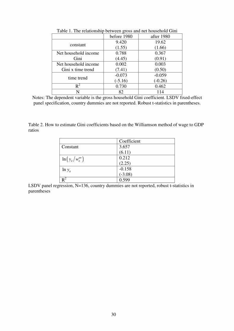
We test this hypothesis for a larger sample of countries in regressions, where we regress the
gross household Gini prior to 1980 (and after 1980) on the net household income Gini, a
trend, a cross effect of trend and net household income Gini.
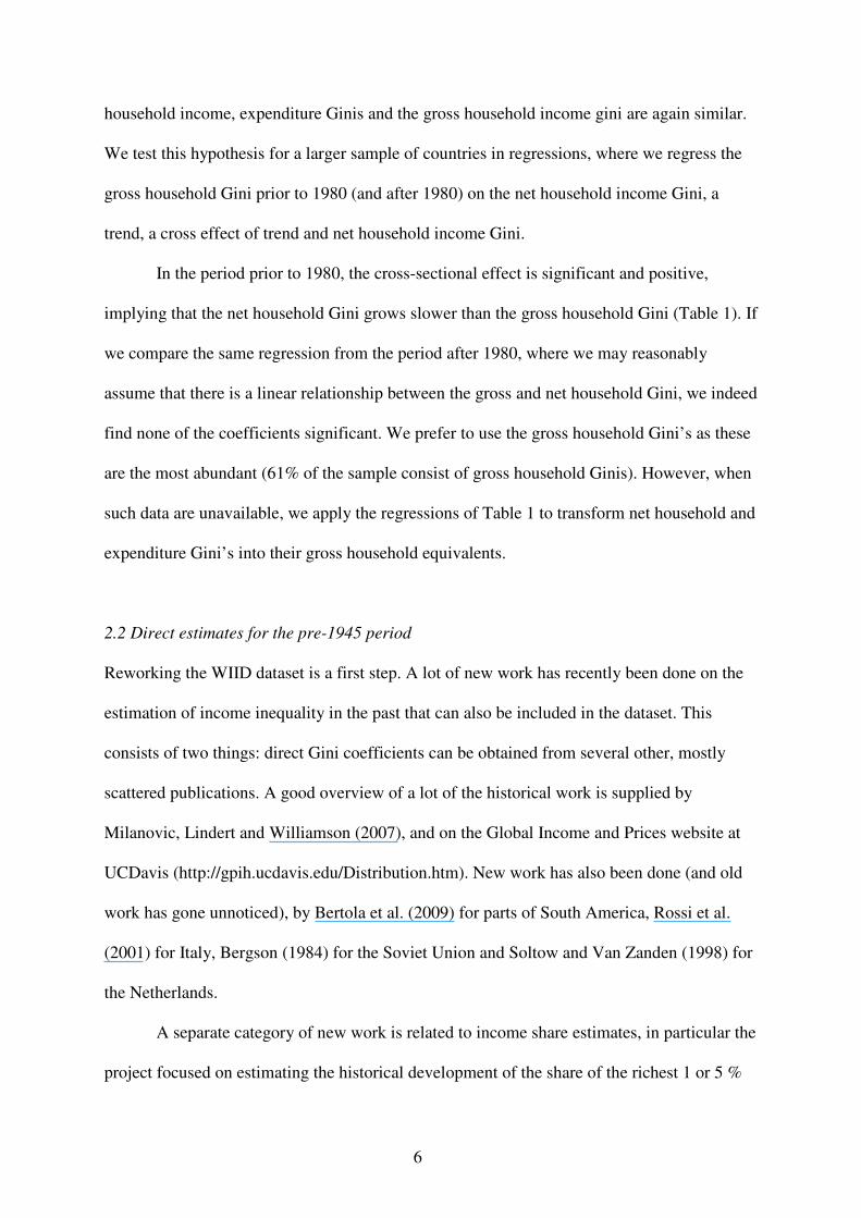
In the period prior to 1980, the cross-sectional effect is significant and positive,
implying that the net household Gini grows slower than the gross household Gini (Table 1). If
we compare the same regression from the period after 1980, where we may reasonably
assume that there is a linear relationship between the gross and net household Gini, we indeed
find none of the coefficients significant. We prefer to use the gross household Gini’s as these
are the most abundant (61% of the sample consist of gross household Ginis). However, when
such data are unavailable, we apply the regressions of Table 1 to transform net household and
expenditure Gini’s into their gross household equivalents.
2.2 Direct estimates for the pre-1945 period
Reworking the WIID dataset is a first step. A lot of new work has recently been done on the
estimation of income inequality in the past that can also be included in the dataset. This
consists of two things: direct Gini coefficients can be obtained from several other, mostly
scattered publications. A good overview of a lot of the historical work is supplied by
Milanovic, Lindert and Williamson (2007), and on the Global Income and Prices website at
UCDavis (http://gpih.ucdavis.edu/Distribution.htm). New work has also been done (and old
work has gone unnoticed), by Bertola et al. (2009) for parts of South America, Rossi et al.
(2001) for Italy, Bergson (1984) for the Soviet Union and Soltow and Van Zanden (1998) for
the Netherlands.
A separate category of new work is related to income share estimates, in particular the
project focused on estimating the historical development of the share of the richest 1 or 5 %
7
in total income, inspired by the work of Piketty and Atkinson.3 One problem, however, is
how to convert these income shares, which are nothing more than just one point on the
Lorenz curve, into Ginis. The only way this can be done is by assuming a distribution. Two
distributions have been proposed - a log-normal and a Pareto distribution – but the literature
suggests that when the whole distribution is covered, the log-normal is to be preferred (see
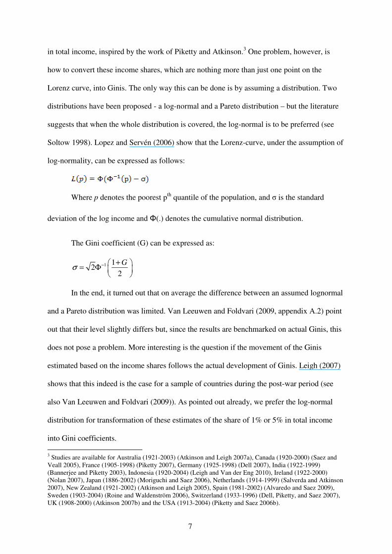
Soltow 1998). Lopez and Servén (2006) show that the Lorenz-curve, under the assumption of
log-normality, can be expressed as follows:
Where p denotes the poorest pth
quantile of the population, and σ is the standard
deviation of the log income and Φ(.) denotes the cumulative normal distribution.
The Gini coefficient (G) can be expressed as:
1 12
2
Gσ − +
= Φ
In the end, it turned out that on average the difference between an assumed lognormal
and a Pareto distribution was limited. Van Leeuwen and Foldvari (2009, appendix A.2) point
out that their level slightly differs but, since the results are benchmarked on actual Ginis, this
does not pose a problem. More interesting is the question if the movement of the Ginis
estimated based on the income shares follows the actual development of Ginis. Leigh (2007)
shows that this indeed is the case for a sample of countries during the post-war period (see
also Van Leeuwen and Foldvari (2009)). As pointed out already, we prefer the log-normal
distribution for transformation of these estimates of the share of 1% or 5% in total income
into Gini coefficients.
3 Studies are available for Australia (1921-2003) (Atkinson and Leigh 2007a), Canada (1920-2000) (Saez and
Veall 2005), France (1905-1998) (Piketty 2007), Germany (1925-1998) (Dell 2007), India (1922-1999)
(Bannerjee and Piketty 2003), Indonesia (1920-2004) (Leigh and Van der Eng 2010), Ireland (1922-2000)
(Nolan 2007), Japan (1886-2002) (Moriguchi and Saez 2006), Netherlands (1914-1999) (Salverda and Atkinson
2007), New Zealand (1921-2002) (Atkinson and Leigh 2005), Spain (1981-2002) (Alvaredo and Saez 2009),
Sweden (1903-2004) (Roine and Waldenström 2006), Switzerland (1933-1996) (Dell, Piketty, and Saez 2007),
UK (1908-2000) (Atkinson 2007b) and the USA (1913-2004) (Piketty and Saez 2006b).
8
2.3 GDP divided by unskilled wages as a proxy
Above two methods give us a reasonable complete picture of income distribution among
countries in the twentieth century. Except for some direct estimates of income inequality
available for a limited number of countries often based on ‘social tables’ not much is known
for the earlier period. For estimates of within country inequality before 1914 we therefore
often have to rely on proxies for income inequality. Several options have been suggested,
such as the income gap between the landed elite and landless labor, or the ratio of average
family income (y) to the annual wage earnings of an unskilled rural laborer (w). Both
methods draw heavily on the concept of the extraction rate (Milanovic et al. 2007). This rate
is defined as the share of total income that is above the subsistence level, which can be
assumed to be equal to the earnings of an unskilled labourer. A high extraction rate – in other
words, a large surplus above subsistence – implies that potentially income inequality can be
very high. The question is which share of this surplus is acquired by the elite.
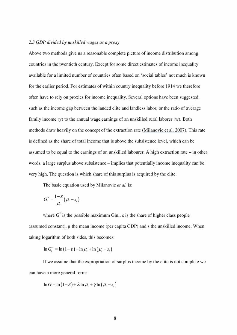
The basic equation used by Milanovic et al. is:
( )* 1t t t
t
G sε
µµ
−= −
where G* is the possible maximum Gini, ε is the share of higher class people
(assumed constant), µ the mean income (per capita GDP) and s the unskilled income. When
taking logarithm of both sides, this becomes:
( ) ( )*ln ln 1 ln lnt t t t
G sε µ µ= − − + −
If we assume that the expropriation of surplus income by the elite is not complete we
can have a more general form:
( ) ( )ln ln 1 ln lnt t t
G sε λ µ γ µ= − + + −
9
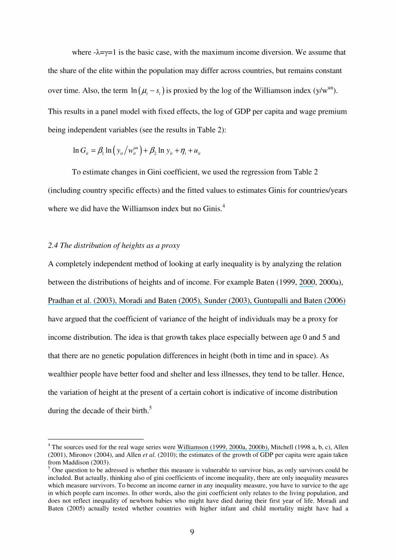
where -λ=γ=1 is the basic case, with the maximum income diversion. We assume that
the share of the elite within the population may differ across countries, but remains constant
over time. Also, the term ( )lnt t
sµ − is proxied by the log of the Williamson index (y/wun
).
This results in a panel model with fixed effects, the log of GDP per capita and wage premium
being independent variables (see the results in Table 2):
( )1 2ln ln lnun
it it it it i itG y w y uβ β η= + + +
To estimate changes in Gini coefficient, we used the regression from Table 2
(including country specific effects) and the fitted values to estimates Ginis for countries/years
where we did have the Williamson index but no Ginis.4
2.4 The distribution of heights as a proxy
A completely independent method of looking at early inequality is by analyzing the relation
between the distributions of heights and of income. For example Baten (1999, 2000, 2000a),
Pradhan et al. (2003), Moradi and Baten (2005), Sunder (2003), Guntupalli and Baten (2006)
have argued that the coefficient of variance of the height of individuals may be a proxy for
income distribution. The idea is that growth takes place especially between age 0 and 5 and
that there are no genetic population differences in height (both in time and in space). As
wealthier people have better food and shelter and less illnesses, they tend to be taller. Hence,
the variation of height at the present of a certain cohort is indicative of income distribution
during the decade of their birth.5
4 The sources used for the real wage series were Williamson (1999, 2000a, 2000b), Mitchell (1998 a, b, c), Allen
(2001), Mironov (2004), and Allen et al. (2010); the estimates of the growth of GDP per capita were again taken
from Maddison (2003). 5 One question to be adressed is whether this measure is vulnerable to survivor bias, as only survivors could be
included. But actually, thinking also of gini coefficients of income inequality, there are only inequality measures
which measure survivors. To become an income earner in any inequality measure, you have to survice to the age
in which people earn incomes. In other words, also the gini coefficient only relates to the living population, and
does not reflect inequality of newborn babies who might have died during their first year of life. Moradi and
Baten (2005) actually tested whether countries with higher infant and child mortality might have had a
10
Heights offer a good complement to conventional inequality indicators and constitute
perhaps an even better indicator in some respect. If the distribution of food and medical
goods in an economy becomes more unequal, heights will also become more unequal. Deaton
(2001) and Pradhan et al. (2003) have argued convincingly that measures of health inequality
are important in their own right, not only in relation to income. Because they do not assume
the existence of a market economy, anthropometric methods can also be used very well for
studying developing countries.
The effects of inequality on heights are best understood by comparing the likely
outcomes of a hypothetical situation, in which a population is exposed to two alternative
allocations of resources A and B after birth:
(A) All individuals receive the same quantity and quality of resources (nutritional and
health inputs). This case refers to a situation of perfect equality.
(B) Available resources are allocated unequally (but independently of the genetic
height potential of the individuals).
In the case of A, the height distribution should only reflect genetic factors. Despite
perfect equality, we observe a biological variance of (normally distributed) heights in this
case. Yet how does the height distribution respond to an increase in inequality (B)? The
unequal allocation of nutritional, medical and shelter resources allows some individuals to
gain and grow taller, while others lose and suffer from decreasing nutritional status. In
comparison with the situation of perfect equality, the individual heights of the rich strata shift
therefore to the right, the poor strata shift to the left. Thus rising inequality should lead to
higher height inequality, although this effect is weakened by the fact that the genetic height
variation accounts for the largest share of height variation. Even a bimodal height distribution
could result if the resource endowment differed extremely between groups. In practice, since
systematically different height CV. They found indeed the expected negative effect. However, only a very small
part of the CV’s variance could be explained by mortality differences between the countries.
11
the biological variance continues to contribute a large share to the total variance, most height
distributions are normally distributed or very close to normal, but with a much higher
standard deviation than A (but see A’Hearn (2004), Jacobs, Katzur and Tassenaar (2008) on
late teenagers).
The coefficient of variation (CV) is the measure most often used in this research.
Baten (1999, 2000a) compared height differences between social groups using the CV for
early 19th
century Bavaria, since an ideal data set was available for this region and time
period, with nearly the entire male population measured at a homogeneous age and the
economic status of all parents recorded. The measures turned out to be highly correlated.
Therefore, high CVs sufficiently reflect social and occupational differences without relying
on classifications.6
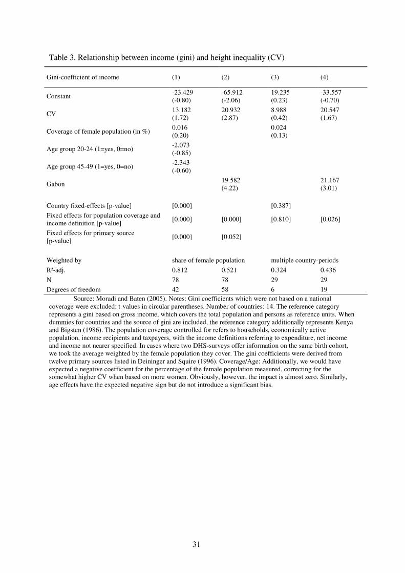
Moradi and Baten (2005) have estimated the relationship between income inequality
and height coefficients of variation (CV) for 14 African countries and 29 five-year periods.
They controlled for the differences in income definition and population coverage by
including dummy variables. In addition, country fixed-effects were included (Table 3, model
1 and 3) which implies that their analysis focused mainly on intertemporal effects. They
found that height CV was significant and positively correlated with the Gini coefficients of
income. An increase in the CV by one unit corresponded with a rise in the Gini coefficient by
13.2 points in the fixed-effects specification. It is noteworthy that the relationship between
the CV and the gini coefficient is not sensitive to country fixed-effects in general. In another
regression without country fixed effects (2), they obtained a coefficient between nutritional
and income inequality of 20.9. Both coefficients were very close to Baten and Fraunholz's
6 The CV of a totally equal society is yet unknown and can only be empirically approximated. For decomposing
world health inequality, Pradhan et al. (2003) tried to standardise height inequality by assuming that the height
distributions in OECD countries reflect the genetic growth potential of individuals only. However, this would
mean that no nutritional and health inequality exists in OECD countries, which seems highly implausible. In
Germany during the 1990s, for example, height differences between social groups were as large as two
centimeters (Baten and Boehm 2009; Komlos and Kriwy 2003). Even in egalitarian Scandinavia, some height
inequality remains between regions (Sunder 2003).
12
(2004) estimate for Latin America, which reported a significant coefficient of 15.5 based on
gini coefficients whose underlying data are of the highest possible quality. Additional
robustness tests including weighting for sample quality confirmed the relationship. Moradi
and Baten (2005) recommended the following formula for translating height CVS into
income Ginis:
(1) Giniit=-33.5+20.5*CVit
They argued that an excellent case for comparing the development of both income and
height-based inequality measures is Kenya, for which the estimates by Bigsten (1985) offer a
consistent source with a sufficient number of data points (Figure 1). The development of both
inequality measures is nearly identical, except for the sudden fall of the gini coefficient in
1955 with which the CV does not correspond. It is actually not clear which of the two
inequality measures describes the development better, but it seems that the CV’s movement
is somewhat smoother and less volatile (the CV might moreover be less volatile due to some
consumption smoothing, as people reduce their savings in harder times to smooth their
consumption). However, both the strong rise of inequality in Kenya during the early 1950s
and the more gradual rise of the late 1960s are clearly visible in both series. Summing up, the
development of height CVs over time serves as a promising measure of inequality, even more
so because in periods and countries in which other data on inequality are either non-existent
or unreliable.
In sum, the relationship between Gini coefficient of income and height CV seems
quite well-established. Hence we collected all available data from hundreds of previously
published articles (see appendix for a list of references), and benefited from scholars who
provided us with their original height data sets. We excluded cases with very small numbers
of height measurements, or if only one special group within a country was included. We took
care that late teenage year / early twenties samples, military truncation, gender, prison
13
selectivity and other factors did not distort our samples. Finally, we calculated the height CV
for each country and birth decade not covered by the income Ginis and converted the CV
with the formula (1) into income Gini equivalents.
2.5 Global inequality
Table 4 gives a summary of the sources of the newly constructed dataset. The overall dataset
consists of 1078 estimates of Gini coefficients of income inequality, spread over more than
130 countries. The greatest number of new estimates is produced by using the height data, but
because these often refer to relatively small countries, the total impact on the estimates of
global inequality that will be presented is more limited. The other new sources of estimates –
‘new’ direct estimates of income inequality, and indirect estimates derived from the
GDP/wage ratio – are more often used for the larger countries. When more than one estimate
for a country was available, we applied the following rules: a direct estimate of income
inequality superseded all indirect estimates, which were in that case ignored; when we had
two different indirect estimates, based on heights and on the GDP/wage ratio, we used more
or less arbitrarily the unweighted average of the two, which happened in 68 cases (Col. 6 of
Table 4). Changing this assumption does not have a big impact on the final results. For
example, using for 1850 the Williamson index only instead of the unweighted average will
increase world income inequality with 1.18%. To get a systematic set of estimates for the
core-group of 30 countries, we had to interpolate a few estimates for those countries.7
The unit of analysis and comparison so far has been the Gini coefficient of the
individual countries. To move from them to global inequality, we (again) had to assume that
7 Estimates are complete for following countries: Belgium, Brazil, China, Spain, France, UK, Indonesia, Italy,
Netherlands, Portugal, Sweden, USA, Germany, India, Poland, Norway, Ghana and Mexico; interpolations were
necessary for Thailand (1850, 1910), Turkey (1850, 1890, 1980), Australia (1820 is assumed to be identical to
1850), Russia/USSR (1850, 1890), Canada (1870), Czechoslovakia (1910), Denmark (1850), Egypt (1890,
1929, and 1820 derived from Turkey) and Peru (1910); for Argentina and Chile in 1820 we did not find a
suitable proxy.
14
the underlying distributions were log-normal, which allows us to translate the Gini coefficient
into an estimate of the whole distribution of income in country X at time Y. This is then
linked to the estimates of the average GDP per capita in the countries concerned.
The growth rate of per capita GDP is calculated from Maddison (2003) whereas the
differences in GDP per capita across countries can be calculated using the Maddison 1990
GK dollars benchmark. Alternatively, recent research by the ICP has resulted in a new set of
PPP’s for 2005 (Worldbank 2008), which are based on a broader set of prices and on data
from much more countries, probably making the 2005 benchmark more reliable than previous
ones. This, and the use of a somewhat different method to estimate the PPP’s, which solves
the problem as noted by Afriat (1967) and more recently by Dowrick and Quiggin (1994),
that PPPs in international prices tend to overestimate the level of real GDP in low income
countries, results in a substantial widening of income disparities between countries (Deaton
and Heston 2008). Yet, since there recently has been some criticisms on the 2005 benchmark
as well, we decided to provide the World Ginis both using the 1990 PPPs as used by
Maddison (2003) and the new 2005 PPPs.
The resulting estimates are reported in Table 5A and 5B for the 1990 and 2005 PPP
benchmarks, the former ones being directly comparable to the estimates of Bourguignon and
Morrisson (2002). Global inequality has two dimensions: within country inequality, which is
the same for these two sets of estimates, and between country inequality. Table 5 also shows
the overlap factor; because of the statistical features of the Gini coefficient, the sum of the
within country Gini and the between country Gini is larger than the global Gini. The
difference between them is the overlap factor, which is in essence nothing more than that
share of the within group inequality of country A that overlaps with within group inequality
of country B. This has led Milanovic (2002, 70) to claim that "the more important the
overlapping component..... the less one's income depends on where she lives" .
15
The effect of moving from 1990 benchmark to the 2005 benchmark is very clear from
these estimates. Yet, both sets show the same pattern of already quite high levels of global
inequality at the start of the period (.54 and .48 respectively). It then increases steeply from
.54 in 1820 to .67 in 1929 and .68 in 1950 according to the 2005 benchmark, after which, in
both sets of estimates, it more or less stabilizes at that (extremely high) level during the
second half of the 20th
century.
Table 6 demonstrates that we normally cover between 85 and 94 percent of global
population with real data, which is quite high; this percentage tends to increase somewhat
during the period under study. On the basis of the Maddison dataset we estimate that the
average income of this 85 to 94 share is only slightly higher than that of the world as a whole,
but the average income of the uncovered rest is clearly lower than of the countries covered by
this experiment (for example, in 1820, the average income of ‘the rest’ can be estimated to be
about 500 1990 international dollars). We therefore more or less consistently underestimate
inequality, but the bias does not change (much) over time.
Compared to Bourguignon and Morrisson (2002), our estimates based on the 1990
benchmark are somewhat lower than theirs, and using the 2005 benchmark substantially
higher by, on average, 4 points on the Gini index. Their estimates of global inequality
increase from a Gini of .50 in 1820 to .61 in 1910, .64 in 1950 and .657 in 1980, whereas the
Gini estimated here range from .48 to.54 in 1820, rises to .59 to .64 in 1910, and .65 to .68 in
1950. After 1950 the B & M estimates continue to increase a bit, whereas our estimates show
more or less stability (with the exception of the estimates for 1975 and 2000, both based on a
more limited number of observations).
3. Error margins
16
Our estimates above are all based on direct information. However, since we use a large
amount of “new” data, and we use a diverse methodology of creating the world income
inequality series, it seems necessary to gauge its imprecision. Basically, our estimates consist
of two components, the within and the between country inequality. Since the within country
inequality is estimated based on several different sets of data, we follow Chapman (1953) and
Feinstein and Thomas (2001) who attach standard errors of 1.25% for firm figures, 3.75% for
good figures, 8.75% for rough estimates, and 20% for conjectures. The actual gross
household Gini’s thus get an error margin of 1.25%, the net household and expenditure Ginis,
which need to be converted into gross household Ginis, get an error margin of 3.75%.
Finally, the Williamson index and height Gini’s are assessed as having a margin of 8.75%.
The results are presented in Table 7: the estimated confidence interval (at 95%) declines
from around 8% in 1820 to 1.4% in 2000.
For the between country inequality, we follow Bourguignon and Morrisson (2002,
730) and run a Monte Carlo simulation (we experimented with this only with the 2005
benchmark data, but using the 1990 benchmark would give very similar results). We assume
100 countries, where the GDP/cap follows an exponential distribution (our empirical
distribution tests showed that in the majority of the cases we cannot reject at 5% that the per
capita GDP followed this probability distribution), and the population follows a lognormal
distribution (again in most cases log-normality seems a very good approximation for
population according to empirical tests [not reported here, but available from the authors]).
For each year we use the parameters estimated from the actual data, and carry out 5000
experiments to estimate the mean, the standard error and the confidence interval of the
between-country Gini. We follow Bourguignon and Morrisson (2002) in assuming that there
is a random (normally distributed) multiplicative measurement error. We apply a mean value
of 1 and 0.2 standard deviations for the error. This 0.2 standard deviation is an absolute
17
maximum since it requires more than double the actual standard deviation in the underlying
data. This results in a 95% confidence interval with about 30% higher or lower Gini (Table
8). Given the strong increase of the between Gini between 1820 and 2000, chances that the
general trend is wrong are quite small.
4. The long-term development of global inequality and poverty
As outlined above, inequality increases between 1820 and 2000 with almost 50%. Most of
these changes, however, occurred before 1950, while inequality remained virtually stable
afterwards. This pattern, however, is largely driven by between country inequality since, as
can be seen in Table 5, within country inequality remained largely constant at .43. This long-
run pattern does not obscure, however, that development was episodic in the short run.
Indeed, within country inequality was essentially constant, except for the period
between ca. 1950-1980 when it fell substantially below the long-run average (from .44 to
.35), followed by an increase in the final decades of the 20th
century, which brings within
inequality, in 2000, back to the level before the ‘egalitarian revolution’ of the 20th
century.
The within country inequality does not contribute a lot to the long run swings in global
inequality. Between country inequality, however, grows strongly between 1820 and 1950.
With the rise of global inequality between 1820 and 1950, the overlap factor increases, but it
then declines between 1950 and 1980, a sign of growing polarization of the income pyramid
discussed below (see Figure 2). This is followed by an increase in the overlap factor again
between 1980 and 2000. What this suggests is that behind the apparent stability of the global
Gini index during the 1950-2000 period, major changes in income distribution occurred,
which express themselves (amongst others) in a changing overlap factor.
18
These changes in the income distribution are also apparent in Figure 2. This Figure
charts the different global income distributions in one picture, indicating both the increase in
income levels, the growth of the population and the changes in its distribution (all in 2005
dollars) (the comparable figure in 2005 prices is very similar). What is in particular striking,
is the change in the structure of the income pyramid through time (see for similar analyses of
the more recent period, see Milanovic 2002, Sala-I-Martin 2006). Between 1820 and 1910,
the world income distribution is unimodal and basically lognormal, although, looking at the
1910 distribution, an extension of its right ´wing´ can already be noticed. In the next few
decades a different distribution emerges with two separate peaks; this is already very clear in
1950 (when the two peaks have almost the same size), and becomes more pronounced in the
1960s and 1970s, when a big gap between rich and poor ‘peaks’ appears. However, in the
1980s and the 1990s the two modes begin to merge, and in 2000 the distribution has become
consistently unimodal again.
One might argue that the switch to a bi-modal distribution is caused by de-
globalization after 1914: a lack of trade caused by two world wars, a depression, and a bi-
polar world system. This, however, is a topic for further research – here we can only
speculate about the fact that this change from a unimodal distribution towards a bi-modal
system is accompanied by the decline of inequality within countries (the ‘egalitarian
revolution’ of the 20th century is a typically phenomenon of the developing nation state,
which allows itself more degrees of freedom in the de-globalized world of 1914-1960). We
can also speculate that after 1980 globalization, the increase of inequality within countries
and the decline of inequality between countries were in a similar way closely interrelated
processes.
19
The dataset also makes it possible to study within country inequality of the main regions of
the world, in order to see to what extent they were affected by these long-term trends. It is
well known that in the post-1950 period there are more or less persistent differences in the
level of within-country income inequality in different regions of the world. Latin America
and Africa have, on average, relatively high levels of inequality, whereas Western Europe
and Asia tend to have lower levels (Deiniger and Squire 1998). These patterns also emerge
when we look at the unweighted averages of the ginis of the different countries in the
different regions and the world as a whole (Table 9): Latin America and Africa almost always
have a higher average Gini than Europe; the Middle East also is often above average, whereas
Asia is usually below average.8 Before 1950 the differences between the continents are
relatively small, however, and Western Europe is still among the regions with, on balance,
above-average inequality. It only moves to below average after 1945. The industrial
revolution therefore emerged in a region with rather high levels of income inequality, but
levels of income were also high there, as a result of which the extraction ratio was much
lower than elsewhere (Milanovic, Lindert and Williamson 2007). This decline of inequality is
even more pronounced in (communist dominated) Eastern Europe, which has by far the
lowest Ginis during the 1950-1990 period. The ‘egalitarian revolution’ of the 20th
century is
also apparent in North America/Australia, and can even be found in the (unweighted) global
averages, which decline between 1929 and 1980 (by about 10%). In all regions we see an
increase in inequality in the last decade of the 20th
century; it is most striking in post
communist Eastern Europe. Before 1950 levels of inequality within these regions are
relatively stable, with the most notable exception of Latin America in the 1870-1910 period,
8 We splitted up the regions according to economic and political characteristics. The first group consists of
Western European countries, consisting of all European countries, except the former socialist ones. Eastern
Europe and the former USSR consist of all former socialist countries of Eastern Europe and the former USSR.
"Asia"consist of all Asian countries, except the Middle East. "Middle East and North Africa" consists of the
Middle Eastern countries and Africa above the Sahara. Sub Saharan Africa contains all other African countries.
Latin America contains all Latin American (and Caribbean) countries. Finally, Western Offshoots, contains
Canada, USA, New Zealand, and Australia.
20
which according to our estimates witnessed a decline of the Gini coefficient by almost 20%
in this period of globalization.
We can also estimate ‘within region’ income inequality of the various parts of the
world, which is the product of inequality within the countries of that region and income
disparities between those countries (for example: it takes into account that within Western
Europe there were large income differences between rich countries such as the UK and the
Netherlands, and poor countries such as Portugal or Finland). This addresses the problem that
countries form the basic unit of analysis in this kind of research, but that their size varies
enormously as well as the problem that income differences across countries may vary widely.
Hence, even when average within country inequality is low, actual inequality may be much
higher because the income differences across countries are higher. Indeed, income inequality
in large countries such as China, the US or India, tends to be higher than that of small,
homogenous countries such as Denmark or Belgium, because it also includes the income
disparities between the different parts of such a large state.
In table 10 we present estimates of ‘within region’ income inequality of 7 regions,
which are, however, still quite different in size (Asia is by far the largest region, with
currently 55 percent of the global population). A number of patterns emerge from these
estimates. In Europe and the Western Offshoots, regional inequality declines in the long run
and moves from the world average to much below that average, but the last two decades of
the 20th
century this process appears to come to an end. Regional inequality in Asia changes
in the opposite direction: it is relatively low during the 19th
century, but increases sharply in
the 20th
century. Increasing ‘within region – between country’ inequality is driving this
process – first Japan is the main mover, later followed by other countries which are
successfully catching up (whereas large parts of the region remain poor). Regional inequality
in Sub-Sahara Africa offers a third pattern: the Gini is very high at the beginning of the
21
period (but the number of observations is quite limited), and continues to be very unequal.
The big gap between the unweighted average Gini of Table 9 and the regional inequality
Gini of Table 10 implies that between country inequality in Africa is quite large, thanks to
some relatively successful economies (South Africa in particular), and many quite
unsuccessful ones (with the lowest GDP per capita’s in the world). In this comparison, it is
not Latin America that comes forward as the most unequal continent (which in other studies
usually is the case); between country inequality is that part of the world is rather limited, as a
result of which ‘within region’ inequality is, initially, even smaller than the unweighted
average of the country-Gini’s. This changes in the course of the 19th
century, but still the
overall level of inequality in the region remains below that of Africa (and of the world as a
whole).
Combining the development of inequality and economic growth, one may estimate the
development of the number of people living below a certain poverty line (of one or two
dollars, in 1990 and 2005 prices). These estimates are made to sketch the long-term changes
in absolute poverty in the world economy (see Table 11). It is important to stress that our
world poverty estimates are lower than most other contemporary estimates. This has two
reasons. First, our world estimates are based on a population weighted average of all
countries in our sample. However, especially some of the poorer regions are
underrepresented. This will bias our estimate of the poor downwards by ca. 6% on average
using one 1990 GK dollars or around 3% in two 1990 GK dollars. Second, we estimate the
number of people with an income below the various thresholds, whereas most studies in this
field focus on expenditure per capita, which is usually lower than income (see for recent
surveys Chen and Ravallion 2008 and Deaton 2010). Indeed, Sala-i-Martin (2006), using the
same combination of data from surveys and average income from national accounts, found
22
roughly similar levels of inequality as in this paper. Ravallion (2004) has shown that both
methods result in roughly similar results provided we accept 2 USD a day as poverty line.
Hence, if one wants to compare our estimate to those in the literature, one best use this
threshold.
Table 11 presents the estimates for the world as a whole in 1990 and 2005
international dollars. According to the 1990 benchmark estimates, the total number of poor
people (below 1 dollar) was more or less stable between 1820 and 1929 (when economic
growth was apparently strong enough to compensate for the growth of the total population),
increased very rapidly between 1929 and 1950 (from 423 to 649 million), fell sharply after
1950 to its lowest point, 222 million, in 1980, but began to increase again after 1980 (a trend
that was only reversed after 1995). A somewhat similar pattern can be found when using 2
dollars per day as the poverty line; using this measure, the number of poor still increases until
1970, declines rapidly between 1970 and 1985, but increases a bit in the next decade. It is
striking that the trends in 2005 dollars are basically the same, although the levels differ a bit.
This is the result of two opposing tendencies: firstly, prices have on average increased from
1990 to 2005, which has the effect of lowering the number of people below the poverty line
(or rather, the poverty line in real terms declines as a result). Secondly, the new 2005 ICP
round increases income disparities between rich and poor countries, which has the opposite
effect of increasing the number of people below the poverty line (although this is more
complex than it seems, as the poverty line is defined by levels of absolute poverty in the poor
countries – see the discussion between Chen and Ravallion 2008 and Deaton 2010). The net
effect of this is the number of poor according to the 2005 benchmark and in 2005 prices are
generally somewhat smaller than according to the 1990 benchmark and in 1990 prices. Our
results are, however, much lower than the most recent estimates made by Chen and Ravallion
(2008) and also different from those published by B&M, who estimated that the number of
23
people living in extreme poverty remained more or less the same between 1960 and 1992. We
on the other hand find a strong decline between 1950 and 1980, followed by relative stability
in more recent years.
Table 12 and 13 summarize the estimates of the distribution of the world’s poor over
different regions. Table 12 shows that poverty is on the decline everywhere, but that the
starting points were very different: in Western Europe and the Western Offshoots, in 1820,
‘only’ one out of four earned less than 1 dollar per day, but this share was three quarter in
Africa – other regions were in between. Latin America saw an almost continuous reduction of
absolute poverty during the 19th
and 20th
century (which only started to stagnate after 1980),
whereas poverty reduction in Asia only began in earnest after 1950 (but it was very rapid
since). The region that had the highest share of poor people in 1820, Sub Sahara Africa, has
also in the long run been rather unsuccessful in reducing the number of inhabitants below the
poverty line. The result of this is, as Table 13 demonstrated, that in 2000 (according to these
estimates) 40-45% of the world’s poor (below the 1 dollar threshold) live in Africa, whereas
the continent only has 11% of the global population.
5. Conclusion
We have reconstructed a new dataset of estimates of the inequality of the income distribution
for a large set of countries for benchmark years starting in 1820 and ending in 2000. This
was, in comparison with the estimates produced by Bourguignon and Morrisson (2002),
based on the use of new (and old) historical studies of income inequality in different
countries, and on different sets of indirect estimates of the development of the Gini index.
From these within country inequality estimates, we aggregated to a World Gini using
income differences between countries. We used the new 2005 PPPs of the ICP project, which
24
may give a more accurate picture of disparities in GDP per capita than the previous ICP
rounds. Since many estimates use the Maddison (2003) data, we also provided a second set of
World Ginis based on these numbers. The combination of these estimates of within and
between country inequality have been used to reconstruct the evolution of global inequality
between 1820 and 2000.
The long term evolution of global inequality that emerges from this is not very
dissimilar from the results presented by B & M. Our estimates show a more or less similar
increase during the 1820-1950 period, and stability (instead of a small increase) during the
second half of the 20th
century. Within country inequality did not change a lot in the very
long run, although in many countries inequality tended to decline during the 20th
century
‘egalitarian revolution’, but this was often followed by a rise of inequality after 1980.
Between country inequality increased a lot and was the main cause behind the very strong
increase in global inequality in these two centuries. This process appears to have come to an
end during the second half of the 20th
century, however – between 1950 and 1980 there was a
high level stagnation of between country inequality, followed by a small decline during the
final decades of the century. This decline in between country inequality between ca 1975 and
2000 was being ‘undone’ however, by the increase of within country inequality in the same
period. In other respects this period of globalization also stands out: whereas global
inequality did not continue to rise, the absolute number of people below the poverty line of
one dollar did not fall anymore after 1980, and even their share in the world population
declined only marginally. The absolute poor therefore did not profit much from globalization
(those with a slightly higher real income, between 1 and 2 dollars per day, did only
marginally better). In the very long-run, however, comparing 1820 with 2000, it looks like
the absolute number of people living below the poverty line remained more or less constant.
25
Our most striking results point to important changes in the structure of global
inequality. It was a clear unimodal distribution in the 19th
century, but it became increasingly
bi-modal during the middle decades of the 20th
century, when a clear separation between
‘rich’ and ‘poor’ peaks in the global income distribution emerged. This is a striking result,
because at the same time, as we saw, the share of the very poor fell rapidly during this period,
both in absolute terms and as a share of the world population. Between 1980 and 2000, the
shape of the global distribution changed ‘suddenly’ from a bi-modal to a unimodal
distribution, mainly due to the rapid growth in countries such as China, India and Indonesia.
Our speculation that these changes in the global income distribution were linked to processes
of globalization and de-globalization in the world economy, clearly require further
explanation. The globalized world of the (late) nineteenth century produced a unimodal
distribution. Processes of de-globalization in the middle decades of the twentieth century had
two effects on global inequality: nation states acquired the freedom to build a welfare state
that sharply reduced income inequality within countries (in the richer part of the world), but
at the same time it seems to have lead to the emergence of a bi-model distribution on a global
scale. The dramatic process of globalization of the final decades of the 20th
century reversed
both changes: it led to a strong increase in within country inequality (bringing it back to its
level from before the ‘egalitarian revolution’ of the twentieth century), and it resulted in the
sudden appearance of a unimodal income distribution on a global scale (and a small decline
in between country inequality).
26
Appendix: heights studies used: http://www.wiwi.uni-
tuebingen.de/cms/fileadmin/Uploads/Schulung/Schulung5/Joerg/ref_anth.pdf
References
Afriat, Sydney (1967), “The construction of utility functions from expenditure data,” International Economic
Review, 8(1), 67–77.
A’Hearn, B. (2004). A Restricted Maximum Likelihood Estimator for Truncated Height Samples. Economics
and Human Biology 2, pp. 5-19
Allen, Robert C. (2001).‘The Great Divergence in European Wages and Prices from the Middle Ages to the
First World War,’ Explorations in Economic History, Vol. 38, pp 411-447.
Allen, Robert & Jean-Pascal Bassino & Debin Ma & Christine Moll-Murata & Jan Luiten van Zanden, 2010.
‘Wages, Prices, and Living Standards in China,1738-1925: in comparison with Europe, Japan, and
India,’ Economic History Review, forthcoming
Alvaredo, F. and Saez, E. (2009). ‘Income and wealth concentration in Spain from a historical and fiscal
perspective,’Journal of the European Economic Association, 7(5), 1140-1167.
Atkinson, A. B. (2007b). ‘Top incomes in the United Kingdom over the twentieth century.’ In Top Incomes over
the Twentieth Century: A Contrast Between Continental European and English Speaking Countries
(ed. A. Atkinson and T. Piketty), pp.82-140. Oxford: Oxford University Press.
Atkinson, A. B. and Leigh, A. (2005). ‘The distribution of top incomes in New Zealand.’
Atkinson, A. B. and Leigh, A. (2007a). ‘The distribution of top incomes in Australia.’
Atkinson, A.B., & Brandolini, A. (2001). Promise and Pitfalls in the Use of ‘Secondary’ Data Sets: Income
Inequality in OECD Countries as a Case Study. Journal of Economic Literature, 39(3), 771-799.
Australian National University CEPR Discussion Paper 503.
Banerjee, A. and T. Piketty (2005), ‘Top Indian Incomes, 1922-2000’, The World Bank Economic Review, 19,
1-20.
Barro, R. J. (2000), ‘Inequality and Growth in a Panel of Countries’, Journal of Economic Growth, vol. 5, no. 1,
March 2000, pp. 5-32.
Bassino, J.P. (2006). Inequality in Japan (1892-1941): Physical Stature, Income, and Health. Economic and
Human Biology 4, pp. 62-88.
Baten, J. (1999). Ernährung und wirtschaftliche Entwicklung in Bayern, 1730-1880. Stuttgart: Steiner.
Baten, J. (2000). "Economic Development and the Distribution of Nutritional Resources in Bavaria, 1797-
1839," in Journal of Income Distribution 9, pp. 89-106
Baten, J. and U. Fraunholz (2004). Did Partial Globalization Increase Inequality? The Case of the Latin
American Periphery, 1950-2000" with Uwe Fraunholz, CESifo Economic Studies 50-1 (2004), pp. 45-
84.
Baten, J., and Böhm, A. (2009). “Trends of Children’s Height and Parental Unemployment: A Large-Scale
Anthropometric Study on Eastern Germany, 1994-2006.”, German Economic Review (forthcoming).
Benabou, R. (1996), ‘Inequality and Growth’, in: B. S. Bernanke and J. J. Rotemberg (eds), NBER
Macroeconomics Annual 1996, Cambridge, MA: MIT Press, pp. 11–74.
Bergson, Abram. (1984). Income inequality under Soviet socialism. Journal of Economic Literature, Vol. 22,
no. 3. September. 1052-1099.
Bertola, Luis, Cecilia Castelnovo, Javier Rodriguez, Henry Willebald (2009). ‘Income distribution in the Latin
American Southern Cone during the first globalization boom and beyond’ International Journal of
Comparative Sociology (forthcoming)
Bigsten, A. (1985). Income Distribution and Growth in a Dual Economy. PhD thesis, Gothenburg University,
Department of Economics.
Bourguignon, F., Morrisson, C.,(2002). Inequality among world citizens: 1890-1992, American Economic
Review 92 (4), 727-744, September.
Brandt, L. & Sands, B. (1992) ‘'Land Concentration and Income Distribution in Republican China,’ in: Chinese
History in Economic Perspective, eds. Th. Rawki and L. Lee, California University Press, Berkeley:
179-206.
Broadberry, S. (2003) “Relative per capita Income Levels in the United Kingdom and the United States since
1870: Reconciling Time Series Projections and Direct Benchmark Estimates”, Journal of Economic
History, 63 (2003): 852-863.
27
Chen, Shoalma and Martin Ravallion (2008) The developing world is poorer than we thought, but no less
successful in the fight against poverty’, Policy Research Working Paper 4703, World Bank.
Chapman, Agatha, L. Wages and Salaries in the United Kingdom 1920–1938. Cambridge: Cambridge
University Press, 1953
Deaton, A. (2001). Relative Deprivation, Inequality and Mortality. NBER Working Paper 8099.
Deaton, A. and A. Heston (2008) ‘Understanding PPPs and PPP-Based National Accounts’. NBER working
paper 14499.
Deaton, A. (2010) ‘Price indexes, inequality, and the measurement of world poverty’, presidential address,
American Economic Association, Atlanta January 2010.
Deininger, K. and Squire, L. (1996), ‘A new dataset measuring income inequality’, The World Bank Economic
Review, 10, 565-591.
Deininger, K. and Squire, L. (1998), ‘New Ways of Looking at Old Issues: Inequality and Growth’, Journal of
Development Economics, December 1998, 57(2), pp. 259 – 87
Dell, F. (2007). ‘Top incomes in Germany throughout the twentieth century: 1891–1998.’ In Top Incomes over
the Twentieth Century: A Contrast Between Continental European and English Speaking Countries
(ed. A. Atkinson and T. Piketty), pp.365-425. Oxford: Oxford University Press.
Dell, F., Piketty T. and Saez, E. (2007). ‘Income and wealth concentration in Switzerland over the 20th century.’
In Top Incomes over the Twentieth Century: A Contrast Between Continental European and English
Speaking Countries (ed. A. Atkinson and T. Piketty), pp.472-500. Oxford: Oxford University Press.
Dowrick, Steve, and John Quiggin, 1994, “International comparisons of living standards and tastes: a revealed
preference approach,” American Economic Review, 84:1, 332–41.
Feinstein, Charles H. and Mark Thomas, ‘A Plea for Errors,’ Discussion Papers in Economic and Social
History, Number 41, University of Oxford 2001.
François, J.F., and H. Rojas-Romagosa (2005), “The Construction and Interpretation of Combined Cross Section
and Time-Series Inequality Datasets,” Worl d Bank Policy Research Working Paper 3748.
Guntupalli, A.M. and Baten, J. (2006). “The Development and Inequality of Heights in North, West and East
India, 1915-44”, Explorations in Economic History 43, iss. 4, pp. 578-608.
Jacobs, J., Katzur, T., Tassenaar, V. (2008). On Estimators for Truncated Height Samples. Economics and
Human Biology 6-1, pp. 43-56.
Jones, C.I., (1997). On the evolution of the world income distribution, Journal of Economic Perspectives 11 (3),
19-36, Summer.
Komlos, J. & Kriwy, P. (2003). The Biological Standard of Living in the Two Germanies. German Economic
Review, 4(4), 459-73.
Komlos, J. (1985). Stature and Nutrition in the Habsburg Monarchy: The Standard of Living and Economic
Development. American Historical Review, 90, 1149-1161.
Latham and H. Kawakatsu (eds.), Asia Pacific Dynamism 1500-2000 (London: Routledge): 13-45.
Leigh, A. (2007) ‘How closely do top income shares track other measures of inequality’, The Economic Journal,
117 (524), F589-F603.
Leigh, A. and Van der Eng P. (2010) ‘Top Incomes in Indonesia, 1920-2004’, in: Top incomes over the
twentieth century: Volume II, A global perspective, eds. Atkinson, A. B, and Piketty, T., Oxford
University Press, Oxford: 171-219.
López, J.H., Servén, L., 2006. A normal relationship? Poverty, growth, and inequality. Macmillan Reference;
New York : Stockton Press, 1998.
Maddison, A. (2001). The world economy: a millennial perspective. OECD, Paris.
Maddison, A. (2003). The world economy: historical statistics. OECD, Paris
Milanovic, B., (2002). True world income distribution, 1988 and 1993: First calculation based on household
surveys alone, Economic Journal 112 (476), 51-92, January.
Milanovic, Branko (2007) World Apart. Measuring International and Global Inequality. Princeton.
Milanovic, Branko (2009) Global Inequality recalculated: the effect of the new 2005 PPP estimates on global
inequality. Policy Research Working Papers 5061, World Bank.
Milanovic, Branko, Peter Lindert and Jeffrey Williamson (2007) Measuring Ancient Inequality. MPRA working
paper No. 5388, http://mpra.ub.uni-muenchen.de/5388/1/MPRA_paper_5388.pdf
Mironov, B. (2004). Prices and Wages in St. Petersburg for Three Centuries (1703-2003). Towards a Global
History of Prices and Wages, Utrecht 19-21 August 2004.
Mitchell, B. R. (2003a). International Historical Statistics: Africa, Asia and Oceania, 1750-2000 (Basingstoke
and New York: Palgrave Macmillan, 4th edn. 2003.
Mitchell, B.R. (1998). International historical statistics: the Americas, 1750-1993, London: Macmillan
Mitchell, B.R. (1998b). International historical statistics: Africa, Asia & Oceania, 1750-1993, London:
Macmillan Reference; New York : Stockton Press, 1998.
Mitchell, B.R. (1998c). International historical statistics: Europe, 1750-1993, London :
28
Moradi, A. and Baten, J. (2005) “Inequality in Sub-Saharan Africa 1950-80: New Estimates and New Results, ”
World Development Volume 33-8 (2005), pp. 1233-1265.
Moriguchi, C. and Saez, E. (2006). ‘The evolution of income concentration in Japan, 1885-2002: evidence from
income tax statistics,’ National Bureau of Economic Research Working Paper 12558, NBER,
Cambridge, MA.
Nolan, B. (2007). ‘Long-term trends in top income shares in Ireland.’ In Top Incomes over the Twentieth
Century: A Contrast Between Continental European and English Speaking Countries (ed. A. Atkinson
and T. Piketty), pp.501-530. Oxford: Oxford University Press.
Persson, T. and Tabellini, G. (1994), ‘Is Inequality Harmful for Growth?’, American Economic Review, 84-3,
pp. 600–21.
Piketty, T. (2007). ‘Income, wage and wealth inequality in France, 1901-1998.’ In Top Incomes over the
Twentieth Century: A Contrast Between Continental European and English Speaking Countries (ed. A.
Atkinson and T. Piketty), pp.43-81. Oxford: Oxford University Press.
Piketty, T. and Saez, E. (2006b). ‘Income inequality in the United States.’ Tables and Figures updated to 2004
in Excel format, http://emlab.berkeley.edu/users/saez/ (downloaded 6 December 2006).
Pradhan, M., Sahn, D.E., & Younger, S.D. (2003). Decomposing World Health Inequality. Journal of Health
Economics, 22(2), 271-293.
Prados de la Escosura, L. (2008), ‘Inequality, Poverty and the Kuznets Curve in Spain, 1850-2000. European
Review of Economic History 12, pp. 287-324
Prados de la Escosura, Leandro, (2000). "International Comparisons of Real Product, 1820-1990: An
Alternative Data Set," Explorations in Economic History, vol. 37(1), pages 1-41, January.
Reference; New York : Stockton Press.
Ravallion, M. (2004) ‘Pessimistic on Poverty?’, The Economist, 371, April 10.
Ravallion, Martin (2010) Price Levels and Economic Growth. Making Sense of the PPP Changes between ICP
Rounds. Policy Research Working Paper, The World Bank, 5229.
Roine, J. and Waldenström, D. (2006). ‘Top incomes in Sweden over the twentieth century.’ Research Institute
of Industrial Economics Working Paper 667, Stockholm, Sweden.
Rossi, N., G. Toniolo, G. Vecchi, “Is the Kuznets curve still alive ? Evidence from Italian household budgets,
1881-1961”, The journal of economic history, 4, 2001.
Saez, E. and Veall, M. (2005). ‘The evolution of high incomes in Northern America: lessons from Canadian
evidence.’ American Economic Review, vol. 95(3), (June), pp. 831-849.
Sala-i-Martin, Xavier (2006). ‘The World Distribution of Income: Falling Povery and … Convergence, Period.’
Quarterly Journal of Economics, May 2006, v. 121, iss. 2, pp. 351-97
Salverda, W. and Atkinson, A. B. (2007). ‘Top incomes in the Netherlands over the twentieth century.’ In Top
Incomes over the Twentieth Century: A Contrast Between Continental European and English Speaking
Countries (ed. A. Atkinson and T. Piketty), pp.426-472. Oxford: Oxford University Press.
Schmitt, L.H. & Harrison, G.A. (1988). Patterns in the Within-Population Variability of Stature and Weight.
Annals of Human Biology, 15(5), 353-364.
Solt, Frederick (2009), “Standardizing the World Income Inequality Database”, Social Science Quarterly, 90
(2), 231-242.
Soltow, L. (1998), “The Measures of Inequality”, in: L. Soltow and J.L. van Zanden (eds.), Income & Wealth
Inequality in the Netherlands 16th-20th Century, Het Spinhuis: Amsterdam, 7-22.
Soltow, Lee and Jan Luiten van Zanden (1998) Income and Wealth Inequality in the Netherlands 1500-1990.
Het Spinhuis Amsterdam
Steckel, R. (1995). Stature and the Standard of Living. Journal of Economic Literature, 33(4), 1903–1940.
Sunder, M. (2003). The Making of Giants in a Welfare State: The Norwegian Experience in the 20th Century.
Economics & Human Biology, 1(2), 267-276.
Terreblanche, S. & De Villiers, R. (2002). A History of Inequality in South Africa, 1652-2002. Pietermaritzburg
: University of Natal Press.
Van Leeuwen, B. & Földvári, P. (2009), “The Development of inequality and poverty in Indonesia, 1932-1999”,
Unpublished paper 2009.
Williamson Jeffrey G. (1998). “Globalization and the Labor Market: Using History to Inform Policy ” pp. 103-
193 in P. Aghion and J. G. Williamson, eds.Growth, Inequality and Globalization. Cambridge UP.
Williamson, J. (1999). Real Wages, Inequality, and Globalization in Latin America Before 1940. Revista de
Historia Economica, 17 (special number), 101-142.
Williamson, J.G. (2000a), ‘Globalization, factor prices and living standards in Asia before 1940’, in A.J.H.
Latham and H. Kawakatsu, eds., Asia Pacific Dynamism 1550-2000, London: Routledge, 13-45.
Williamson, J. (2000b). Real Wages and Factor Prices Around the Mediterranean 1500-1940,in S. Pamuk and
J.G. Williamson (eds.) The Mediterranean Response to Globalization Before 1950 (London:
Routledge) : 45-75.
29
Williamson, J. G. and P. H. Lindert (1980), American Inequality: A Macroeconomic History. (New York:
Academic Press).
World Bank (2008), Global purchasing power parities and real expenditures: 2005 international comparison
program, Washington, DC.World Bank Policy Research Working Paper 3814.
World Income Inequality Database V2.0c May 2008
(http://www.wider.unu.edu/research/Database/en_GB/database/)
30
Table 1. The relationship between gross and net household Gini
before 1980 after 1980
constant 9.420
(1.55)
19.62
(1.66)
Net household income
Gini
0.788
(4.45)
0.367
(0.91)
Net household income
Gini x time trend
0.002
(7.41)
0.003
(0.50)
time trend -0.073
(-5.16)
-0.059
(-0.26)
R2
0.730 0.462
N 82 114
Notes: The dependent variable is the gross household Gini coefficient. LSDV fixed-effect
panel specification, country dummies are not reported. Robust t-statistics in parentheses.
Table 2. How to estimate Gini coefficients based on the Williamson method of wage to GDP
ratios
Coefficient
Constant 3.657
(6.11)
( )ln un
it ity w 0.212
(2.25)
ln ity -0.158
(-3.08)
R2
0.599
LSDV panel regression, N=136, country dummies are not reported, robust t-statistics in
parentheses
31
Table 3. Relationship between income (gini) and height inequality (CV)
Gini-coefficient of income (1) (2) (3) (4)
Constant -23.429
(-0.80)
-65.912
(-2.06)
19.235
(0.23)
-33.557
(-0.70)
CV 13.182
(1.72)
20.932
(2.87)
8.988
(0.42)
20.547
(1.67)
Coverage of female population (in %) 0.016
(0.20)
0.024
(0.13)
Age group 20-24 (1=yes, 0=no) -2.073
(-0.85)
Age group 45-49 (1=yes, 0=no) -2.343
(-0.60)
Gabon 19.582
(4.22)
21.167
(3.01)
Country fixed-effects [p-value] [0.000] [0.387]
Fixed effects for population coverage and
income definition [p-value] [0.000] [0.000] [0.810] [0.026]
Fixed effects for primary source
[p-value] [0.000] [0.052]
Weighted by share of female population multiple country-periods
R²-adj. 0.812 0.521 0.324 0.436
N 78 78 29 29
Degrees of freedom 42 58 6 19
Source: Moradi and Baten (2005). Notes: Gini coefficients which were not based on a national
coverage were excluded; t-values in circular parentheses. Number of countries: 14. The reference category
represents a gini based on gross income, which covers the total population and persons as reference units. When
dummies for countries and the source of gini are included, the reference category additionally represents Kenya
and Bigsten (1986). The population coverage controlled for refers to households, economically active
population, income recipients and taxpayers, with the income definitions referring to expenditure, net income
and income not nearer specified. In cases where two DHS-surveys offer information on the same birth cohort,
we took the average weighted by the female population they cover. The gini coefficients were derived from
twelve primary sources listed in Deininger and Squire (1996). Coverage/Age: Additionally, we would have
expected a negative coefficient for the percentage of the female population measured, correcting for the
somewhat higher CV when based on more women. Obviously, however, the impact is almost zero. Similarly,
age effects have the expected negative sign but do not introduce a significant bias.
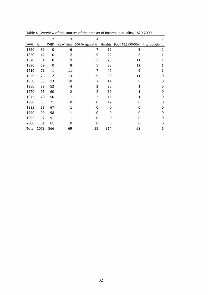
32
Table 4. Overview of the sources of the dataset of income inequality, 1820-2000
1 2 3 4 5 6 7
year All WIID ‘New’ ginis GDP/wage ratio Heights Both 4&5 (50/50) Interpolations
1820 39 0 6 7 19 5 2
1850 42 0 2 9 22 8 1
1870 54 0 9 5 28 11 1
1890 59 0 8 5 33 12 1
1910 71 1 11 7 42 9 1
1929 73 2 13 9 38 11 0
1950 83 13 10 7 44 9 0
1960 89 52 4 2 30 1 0
1970 95 60 2 2 30 1 0
1975 70 50 1 2 16 1 0
1980 83 71 0 0 12 0 0
1985 68 67 1 0 0 0 0
1990 99 98 1 0 0 0 0
1995 92 91 1 0 0 0 0
2000 61 61 0 0 0 0 0
Total 1078 566 69 55 314 68 6
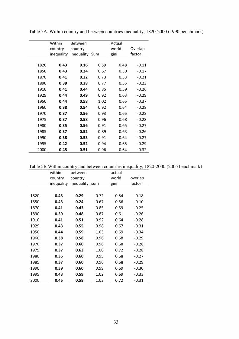
33
Table 5A. Within country and between countries inequality, 1820-2000 (1990 benchmark)
Within
country
inequality
Between
country
inequality Sum
Actual
world
gini
Overlap
factor
1820 0.43 0.16 0.59 0.48 -0.11
1850 0.43 0.24 0.67 0.50 -0.17
1870 0.41 0.32 0.73 0.53 -0.21
1890 0.39 0.38 0.77 0.55 -0.23
1910 0.41 0.44 0.85 0.59 -0.26
1929 0.44 0.49 0.92 0.63 -0.29
1950 0.44 0.58 1.02 0.65 -0.37
1960 0.38 0.54 0.92 0.64 -0.28
1970 0.37 0.56 0.93 0.65 -0.28
1975 0.37 0.58 0.96 0.68 -0.28
1980 0.35 0.56 0.91 0.65 -0.27
1985 0.37 0.52 0.89 0.63 -0.26
1990 0.38 0.53 0.91 0.64 -0.27
1995 0.42 0.52 0.94 0.65 -0.29
2000 0.45 0.51 0.96 0.64 -0.32
Table 5B Within country and between countries inequality, 1820-2000 (2005 benchmark)
within
country
inequality
between
country
inequality sum
actual
world
gini
overlap
factor
1820 0.43 0.29 0.72 0.54 -0.18
1850 0.43 0.24 0.67 0.56 -0.10
1870 0.41 0.43 0.85 0.59 -0.25
1890 0.39 0.48 0.87 0.61 -0.26
1910 0.41 0.51 0.92 0.64 -0.28
1929 0.43 0.55 0.98 0.67 -0.31
1950 0.44 0.59 1.03 0.69 -0.34
1960 0.38 0.58 0.96 0.68 -0.29
1970 0.37 0.60 0.96 0.68 -0.28
1975 0.37 0.63 1.00 0.72 -0.28
1980 0.35 0.60 0.95 0.68 -0.27
1985 0.37 0.60 0.96 0.68 -0.29
1990 0.39 0.60 0.99 0.69 -0.30
1995 0.43 0.59 1.02 0.69 -0.33
2000 0.45 0.58 1.03 0.72 -0.31
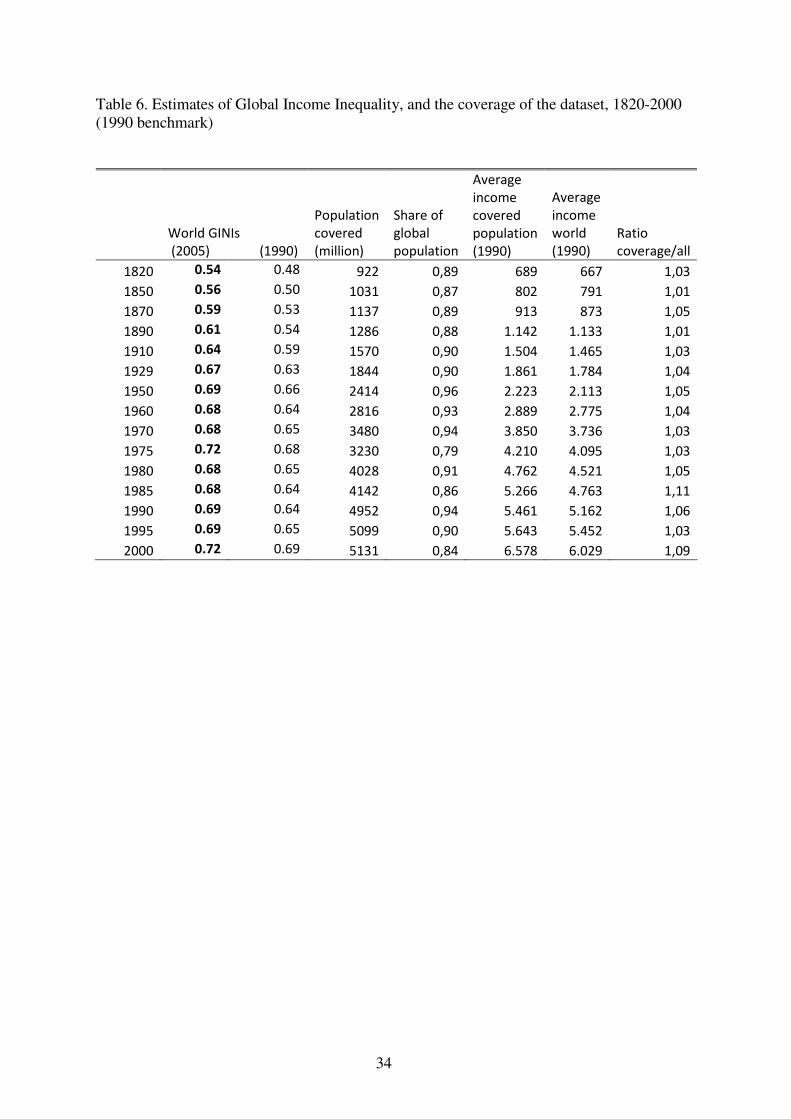
34
Table 6. Estimates of Global Income Inequality, and the coverage of the dataset, 1820-2000
(1990 benchmark)
World GINIs
(2005) (1990)
Population
covered
(million)
Share of
global
population
Average
income
covered
population
(1990)
Average
income
world
(1990)
Ratio
coverage/all
1820 0.54 0.48 922 0,89 689 667 1,03
1850 0.56 0.50 1031 0,87 802 791 1,01
1870 0.59 0.53 1137 0,89 913 873 1,05
1890 0.61 0.54 1286 0,88 1.142 1.133 1,01
1910 0.64 0.59 1570 0,90 1.504 1.465 1,03
1929 0.67 0.63 1844 0,90 1.861 1.784 1,04
1950 0.69 0.66 2414 0,96 2.223 2.113 1,05
1960 0.68 0.64 2816 0,93 2.889 2.775 1,04
1970 0.68 0.65 3480 0,94 3.850 3.736 1,03
1975 0.72 0.68 3230 0,79 4.210 4.095 1,03
1980 0.68 0.65 4028 0,91 4.762 4.521 1,05
1985 0.68 0.64 4142 0,86 5.266 4.763 1,11
1990 0.69 0.64 4952 0,94 5.461 5.162 1,06
1995 0.69 0.65 5099 0,90 5.643 5.452 1,03
2000 0.72 0.69 5131 0,84 6.578 6.029 1,09
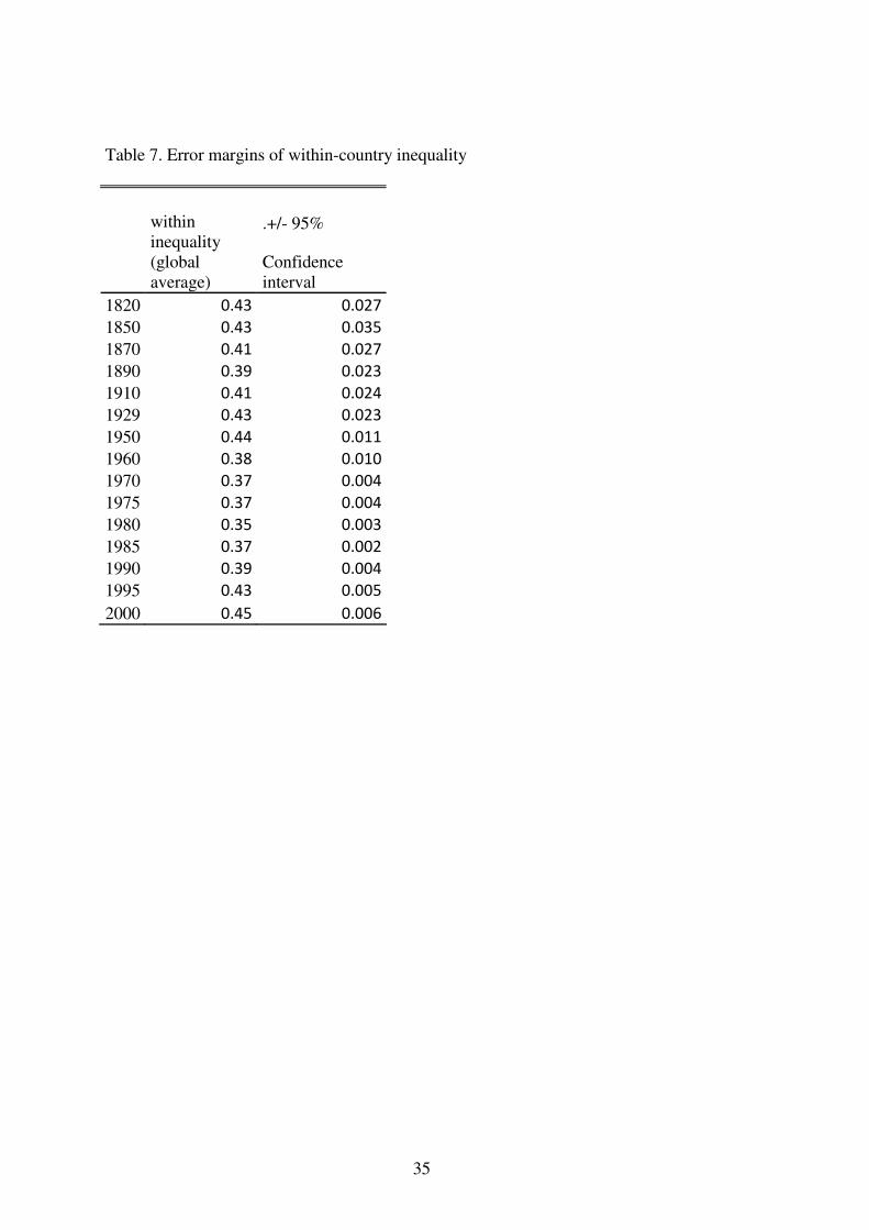
35
Table 7. Error margins of within-country inequality
.+/- 95%
within
inequality
(global
average)
Confidence
interval
1820 0.43 0.027
1850 0.43 0.035
1870 0.41 0.027
1890 0.39 0.023
1910 0.41 0.024
1929 0.43 0.023
1950 0.44 0.011
1960 0.38 0.010
1970 0.37 0.004
1975 0.37 0.004
1980 0.35 0.003
1985 0.37 0.002
1990 0.39 0.004
1995 0.43 0.005
2000 0.45 0.006
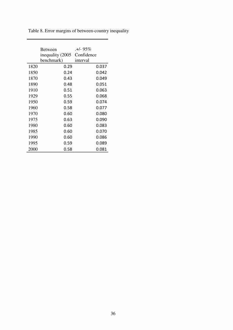
36
Table 8. Error margins of between-country inequality
.+/- 95%
Between
inequality (2005
benchmark)
Confidence
interval
1820 0.29 0.037
1850 0.24 0.042
1870 0.43 0.049
1890 0.48 0.051
1910 0.51 0.063
1929 0.55 0.068
1950 0.59 0.074
1960 0.58 0.077
1970 0.60 0.080
1975 0.63 0.090
1980 0.60 0.083
1985 0.60 0.070
1990 0.60 0.086
1995 0.59 0.089
2000 0.58 0.081
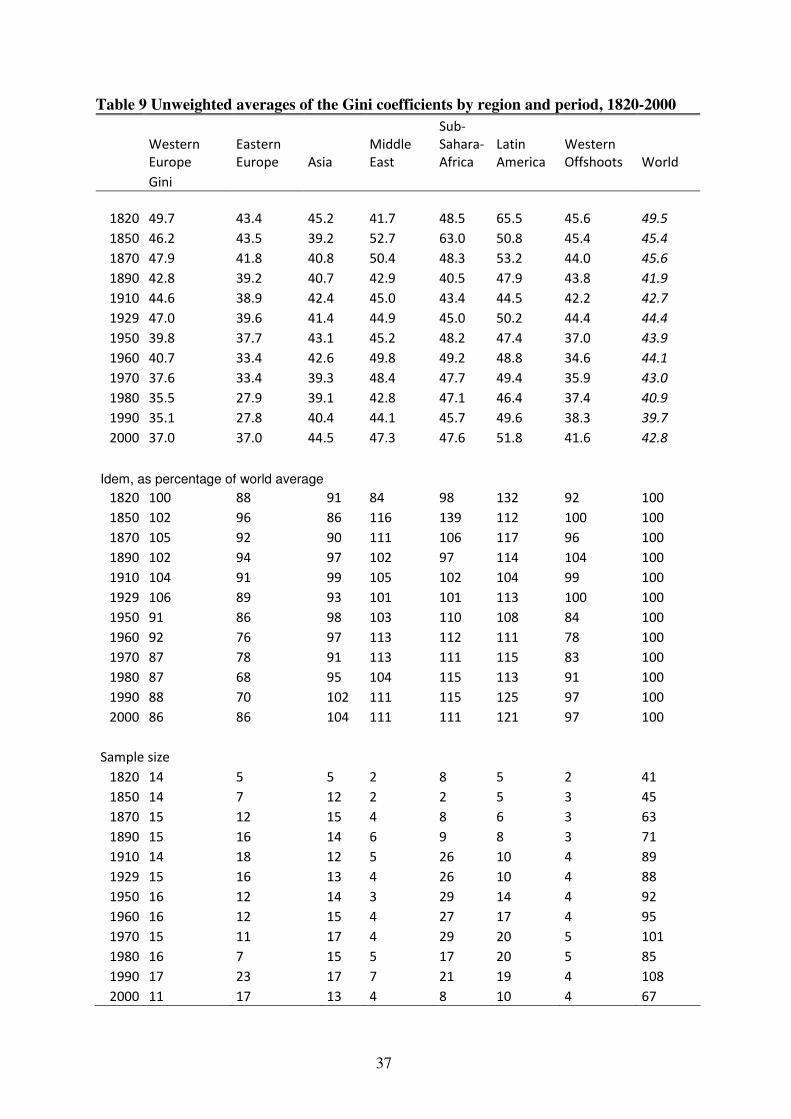
37
Table 9 Unweighted averages of the Gini coefficients by region and period, 1820-2000
Western
Europe
Eastern
Europe Asia
Middle
East
Sub-
Sahara-
Africa
Latin
America
Western
Offshoots World
Gini
1820 49.7 43.4
45.2 41.7 48.5 65.5 45.6 49.5
1850 46.2 43.5 39.2 52.7 63.0 50.8 45.4 45.4
1870 47.9 41.8 40.8 50.4 48.3 53.2 44.0 45.6
1890 42.8 39.2 40.7 42.9 40.5 47.9 43.8 41.9
1910 44.6 38.9 42.4 45.0 43.4 44.5 42.2 42.7
1929 47.0 39.6 41.4 44.9 45.0 50.2 44.4 44.4
1950 39.8 37.7 43.1 45.2 48.2 47.4 37.0 43.9
1960 40.7 33.4 42.6 49.8 49.2 48.8 34.6 44.1
1970 37.6 33.4 39.3 48.4 47.7 49.4 35.9 43.0
1980 35.5 27.9 39.1 42.8 47.1 46.4 37.4 40.9
1990 35.1 27.8 40.4 44.1 45.7 49.6 38.3 39.7
2000 37.0 37.0 44.5 47.3 47.6 51.8 41.6 42.8
Idem, as percentage of world average
1820 100 88 91 84 98 132 92 100
1850 102 96 86 116 139 112 100 100
1870 105 92 90 111 106 117 96 100
1890 102 94 97 102 97 114 104 100
1910 104 91 99 105 102 104 99 100
1929 106 89 93 101 101 113 100 100
1950 91 86 98 103 110 108 84 100
1960 92 76 97 113 112 111 78 100
1970 87 78 91 113 111 115 83 100
1980 87 68 95 104 115 113 91 100
1990 88 70 102 111 115 125 97 100
2000 86 86 104 111 111 121 97 100
Sample size
1820 14 5 5 2 8 5 2 41
1850 14 7 12 2 2 5 3 45
1870 15 12 15 4 8 6 3 63
1890 15 16 14 6 9 8 3 71
1910 14 18 12 5 26 10 4 89
1929 15 16 13 4 26 10 4 88
1950 16 12 14 3 29 14 4 92
1960 16 12 15 4 27 17 4 95
1970 15 11 17 4 29 20 5 101
1980 16 7 15 5 17 20 5 85
1990 17 23 17 7 21 19 4 108
2000 11 17 13 4 8 10 4 67
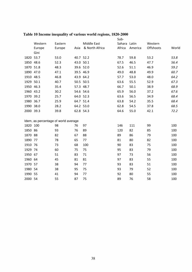
38
Table 10 Income inequality of various world regions, 1820-2000
Western
Europe
Eastern
Europe Asia
Middle East
& North Africa
Sub-
Sahara
Africa
Latin
America
Western
Offshoots World
Gini
1820 53.7 53.0 40.7 52.2 78.7 59.8 53.2 53.8
1850 48.6 52.3 43.0 50.1 67.5 46.5 47.7 56.4
1870 51.8 48.3 39.6 52.0 52.6 51.1 46.9 59.2
1890 47.0 47.1 39.5 46.9 49.0 48.8 49.9 60.7
1910 48.5 46.8 43.9 64.2 57.7 53.0 48.0 64.2
1929 50.1 40.7 50.5 50.5 63.6 55.5 52.9 67.3
1950 46.3 35.4 57.3 48.7 66.7 50.1 38.9 68.9
1960 43.2 30.2 54.6 54.6 65.9 56.0 37.2 67.6
1970 39.2 25.7 64.0 52.3 63.6 56.5 34.9 68.4
1980 36.7 25.9 64.7 51.4 63.8 54.2 35.5 68.4
1990 38.0 28.2 64.2 53.0 62.8 54.5 37.8 68.5
2000 39.3 39.8 62.8 54.3 64.6 55.0 42.1 72.2
Idem, as percentage of world average
1820 100 98 76 97 146 111 99 100
1850 86 93 76 89 120 82 85 100
1870 88 82 67 88 89 86 79 100
1890 77 78 65 77 81 80 82 100
1910 76 73 68 100 90 83 75 100
1929 74 60 75 75 95 83 79 100
1950 67 51 83 71 97 73 56 100
1960 64 45 81 81 97 83 55 100
1970 57 38 94 77 93 83 51 100
1980 54 38 95 75 93 79 52 100
1990 55 41 94 77 92 80 55 100
2000 54 55 87 75 89 76 58 100
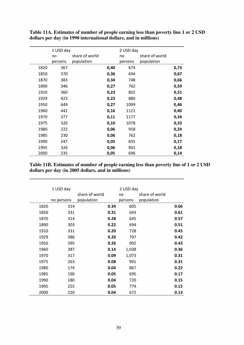
39
Table 11A. Estimates of number of people earning less than poverty line 1 or 2 USD
dollars per day (in 1990 international dollars, and in millions)
1 USD day 2 USD day
no
persons
share of world
population
no
persons
share of world
population
1820 367 0,40 674 0,73
1850 370 0,36 694 0,67
1870 383 0,34 748 0,66
1890 346 0,27 762 0,59
1910 360 0,23 802 0,51
1929 423 0,23 880 0,48
1950 649 0,27 1099 0,46
1960 442 0,16 1121 0,40
1970 377 0,11 1177 0,34
1975 320 0,10 1078 0,33
1980 222 0,06 958 0,24
1985 230 0,06 762 0,18
1990 247 0,05 835 0,17
1995 326 0,06 901 0,18
2000 235 0,05 696 0,14
Table 11B. Estimates of number of people earning less than poverty line of 1 or 2 USD
dollars per day (in 2005 dollars, and in millions)
1 USD day 2 USD day
no persons
share of world
population
no
persons
share of world
population
1820 314 0.34 605 0.66
1850 331 0.31 643 0.61
1870 314 0.28 645 0.57
1890 303 0.22 694 0.51
1910 331 0.20 728 0.45
1929 386 0.20 797 0.42
1950 595 0.26 992 0.43
1960 387 0.14 1,038 0.36
1970 317 0.09 1,073 0.31
1975 263 0.08 991 0.31
1980 174 0.04 867 0.22
1985 190 0.05 695 0.17
1990 180 0.04 720 0.15
1995 255 0.05 774 0.15
2000 220 0.04 672 0.13
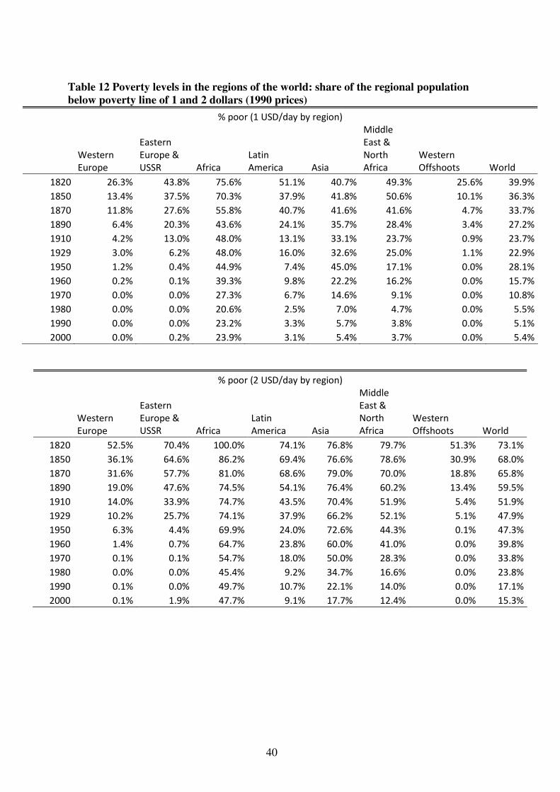
40
Table 12 Poverty levels in the regions of the world: share of the regional population
below poverty line of 1 and 2 dollars (1990 prices)
% poor (1 USD/day by region)
Western
Europe
Eastern
Europe &
USSR Africa
Latin
America Asia
Middle
East &
North
Africa
Western
Offshoots World
1820 26.3% 43.8% 75.6% 51.1% 40.7% 49.3% 25.6% 39.9%
1850 13.4% 37.5% 70.3% 37.9% 41.8% 50.6% 10.1% 36.3%
1870 11.8% 27.6% 55.8% 40.7% 41.6% 41.6% 4.7% 33.7%
1890 6.4% 20.3% 43.6% 24.1% 35.7% 28.4% 3.4% 27.2%
1910 4.2% 13.0% 48.0% 13.1% 33.1% 23.7% 0.9% 23.7%
1929 3.0% 6.2% 48.0% 16.0% 32.6% 25.0% 1.1% 22.9%
1950 1.2% 0.4% 44.9% 7.4% 45.0% 17.1% 0.0% 28.1%
1960 0.2% 0.1% 39.3% 9.8% 22.2% 16.2% 0.0% 15.7%
1970 0.0% 0.0% 27.3% 6.7% 14.6% 9.1% 0.0% 10.8%
1980 0.0% 0.0% 20.6% 2.5% 7.0% 4.7% 0.0% 5.5%
1990 0.0% 0.0% 23.2% 3.3% 5.7% 3.8% 0.0% 5.1%
2000 0.0% 0.2% 23.9% 3.1% 5.4% 3.7% 0.0% 5.4%
% poor (2 USD/day by region)
Western
Europe
Eastern
Europe &
USSR Africa
Latin
America Asia
Middle
East &
North
Africa
Western
Offshoots World
1820 52.5% 70.4% 100.0% 74.1% 76.8% 79.7% 51.3% 73.1%
1850 36.1% 64.6% 86.2% 69.4% 76.6% 78.6% 30.9% 68.0%
1870 31.6% 57.7% 81.0% 68.6% 79.0% 70.0% 18.8% 65.8%
1890 19.0% 47.6% 74.5% 54.1% 76.4% 60.2% 13.4% 59.5%
1910 14.0% 33.9% 74.7% 43.5% 70.4% 51.9% 5.4% 51.9%
1929 10.2% 25.7% 74.1% 37.9% 66.2% 52.1% 5.1% 47.9%
1950 6.3% 4.4% 69.9% 24.0% 72.6% 44.3% 0.1% 47.3%
1960 1.4% 0.7% 64.7% 23.8% 60.0% 41.0% 0.0% 39.8%
1970 0.1% 0.1% 54.7% 18.0% 50.0% 28.3% 0.0% 33.8%
1980 0.0% 0.0% 45.4% 9.2% 34.7% 16.6% 0.0% 23.8%
1990 0.1% 0.0% 49.7% 10.7% 22.1% 14.0% 0.0% 17.1%
2000 0.1% 1.9% 47.7% 9.1% 17.7% 12.4% 0.0% 15.3%
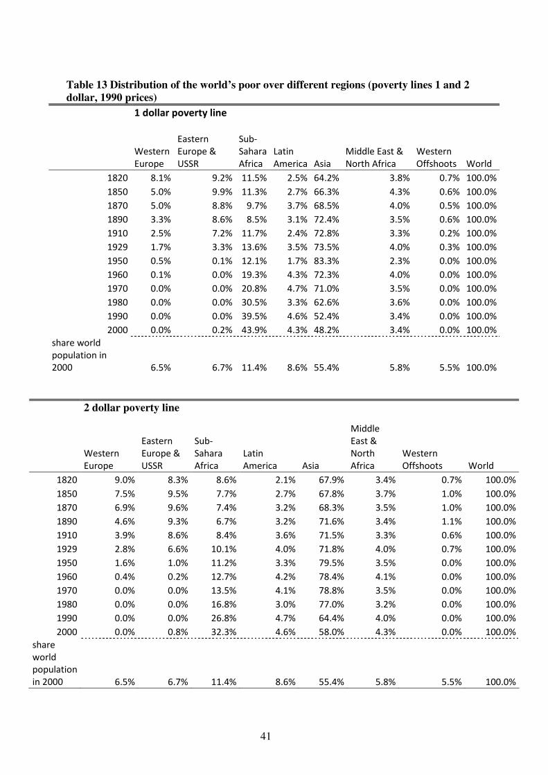
41
Table 13 Distribution of the world’s poor over different regions (poverty lines 1 and 2
dollar, 1990 prices)
1 dollar poverty line
Western
Europe
Eastern
Europe &
USSR
Sub-
Sahara
Africa
Latin
America Asia
Middle East &
North Africa
Western
Offshoots World
1820 8.1% 9.2% 11.5% 2.5% 64.2% 3.8% 0.7% 100.0%
1850 5.0% 9.9% 11.3% 2.7% 66.3% 4.3% 0.6% 100.0%
1870 5.0% 8.8% 9.7% 3.7% 68.5% 4.0% 0.5% 100.0%
1890 3.3% 8.6% 8.5% 3.1% 72.4% 3.5% 0.6% 100.0%
1910 2.5% 7.2% 11.7% 2.4% 72.8% 3.3% 0.2% 100.0%
1929 1.7% 3.3% 13.6% 3.5% 73.5% 4.0% 0.3% 100.0%
1950 0.5% 0.1% 12.1% 1.7% 83.3% 2.3% 0.0% 100.0%
1960 0.1% 0.0% 19.3% 4.3% 72.3% 4.0% 0.0% 100.0%
1970 0.0% 0.0% 20.8% 4.7% 71.0% 3.5% 0.0% 100.0%
1980 0.0% 0.0% 30.5% 3.3% 62.6% 3.6% 0.0% 100.0%
1990 0.0% 0.0% 39.5% 4.6% 52.4% 3.4% 0.0% 100.0%
2000 0.0% 0.2% 43.9% 4.3% 48.2% 3.4% 0.0% 100.0%
share world
population in
2000 6.5% 6.7% 11.4% 8.6% 55.4% 5.8% 5.5% 100.0%
2 dollar poverty line
Western
Europe
Eastern
Europe &
USSR
Sub-
Sahara
Africa
Latin
America Asia
Middle
East &
North
Africa
Western
Offshoots World
1820 9.0% 8.3% 8.6% 2.1% 67.9% 3.4% 0.7% 100.0%
1850 7.5% 9.5% 7.7% 2.7% 67.8% 3.7% 1.0% 100.0%
1870 6.9% 9.6% 7.4% 3.2% 68.3% 3.5% 1.0% 100.0%
1890 4.6% 9.3% 6.7% 3.2% 71.6% 3.4% 1.1% 100.0%
1910 3.9% 8.6% 8.4% 3.6% 71.5% 3.3% 0.6% 100.0%
1929 2.8% 6.6% 10.1% 4.0% 71.8% 4.0% 0.7% 100.0%
1950 1.6% 1.0% 11.2% 3.3% 79.5% 3.5% 0.0% 100.0%
1960 0.4% 0.2% 12.7% 4.2% 78.4% 4.1% 0.0% 100.0%
1970 0.0% 0.0% 13.5% 4.1% 78.8% 3.5% 0.0% 100.0%
1980 0.0% 0.0% 16.8% 3.0% 77.0% 3.2% 0.0% 100.0%
1990 0.0% 0.0% 26.8% 4.7% 64.4% 4.0% 0.0% 100.0%
2000 0.0% 0.8% 32.3% 4.6% 58.0% 4.3% 0.0% 100.0%
share
world
population
in 2000 6.5% 6.7% 11.4% 8.6% 55.4% 5.8% 5.5% 100.0%
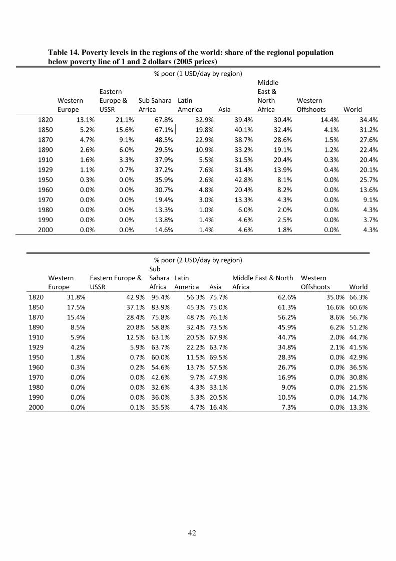
42
Table 14. Poverty levels in the regions of the world: share of the regional population
below poverty line of 1 and 2 dollars (2005 prices)
% poor (1 USD/day by region)
Western
Europe
Eastern
Europe &
USSR
Sub Sahara
Africa
Latin
America Asia
Middle
East &
North
Africa
Western
Offshoots World
1820 13.1% 21.1% 67.8% 32.9% 39.4% 30.4% 14.4% 34.4%
1850 5.2% 15.6% 67.1% 19.8% 40.1% 32.4% 4.1% 31.2%
1870 4.7% 9.1% 48.5% 22.9% 38.7% 28.6% 1.5% 27.6%
1890 2.6% 6.0% 29.5% 10.9% 33.2% 19.1% 1.2% 22.4%
1910 1.6% 3.3% 37.9% 5.5% 31.5% 20.4% 0.3% 20.4%
1929 1.1% 0.7% 37.2% 7.6% 31.4% 13.9% 0.4% 20.1%
1950 0.3% 0.0% 35.9% 2.6% 42.8% 8.1% 0.0% 25.7%
1960 0.0% 0.0% 30.7% 4.8% 20.4% 8.2% 0.0% 13.6%
1970 0.0% 0.0% 19.4% 3.0% 13.3% 4.3% 0.0% 9.1%
1980 0.0% 0.0% 13.3% 1.0% 6.0% 2.0% 0.0% 4.3%
1990 0.0% 0.0% 13.8% 1.4% 4.6% 2.5% 0.0% 3.7%
2000 0.0% 0.0% 14.6% 1.4% 4.6% 1.8% 0.0% 4.3%
% poor (2 USD/day by region)
Western
Europe
Eastern Europe &
USSR
Sub
Sahara
Africa
Latin
America Asia
Middle East & North
Africa
Western
Offshoots World
1820 31.8% 42.9% 95.4% 56.3% 75.7% 62.6% 35.0% 66.3%
1850 17.5% 37.1% 83.9% 45.3% 75.0% 61.3% 16.6% 60.6%
1870 15.4% 28.4% 75.8% 48.7% 76.1% 56.2% 8.6% 56.7%
1890 8.5% 20.8% 58.8% 32.4% 73.5% 45.9% 6.2% 51.2%
1910 5.9% 12.5% 63.1% 20.5% 67.9% 44.7% 2.0% 44.7%
1929 4.2% 5.9% 63.7% 22.2% 63.7% 34.8% 2.1% 41.5%
1950 1.8% 0.7% 60.0% 11.5% 69.5% 28.3% 0.0% 42.9%
1960 0.3% 0.2% 54.6% 13.7% 57.5% 26.7% 0.0% 36.5%
1970 0.0% 0.0% 42.6% 9.7% 47.9% 16.9% 0.0% 30.8%
1980 0.0% 0.0% 32.6% 4.3% 33.1% 9.0% 0.0% 21.5%
1990 0.0% 0.0% 36.0% 5.3% 20.5% 10.5% 0.0% 14.7%
2000 0.0% 0.1% 35.5% 4.7% 16.4% 7.3% 0.0% 13.3%
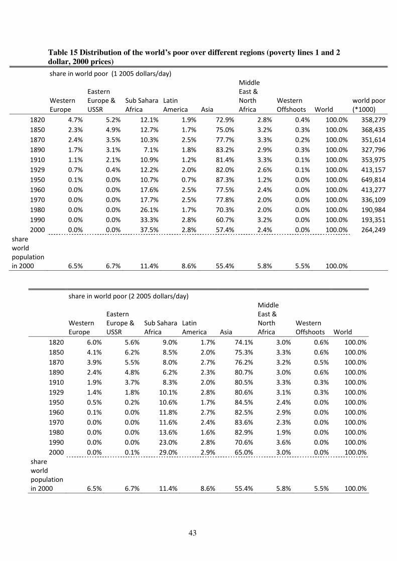
43
Table 15 Distribution of the world’s poor over different regions (poverty lines 1 and 2
dollar, 2000 prices)
share in world poor (1 2005 dollars/day)
Western
Europe
Eastern
Europe &
USSR
Sub Sahara
Africa
Latin
America Asia
Middle
East &
North
Africa
Western
Offshoots World
world poor
(*1000)
1820 4.7% 5.2% 12.1% 1.9% 72.9% 2.8% 0.4% 100.0% 358,279
1850 2.3% 4.9% 12.7% 1.7% 75.0% 3.2% 0.3% 100.0% 368,435
1870 2.4% 3.5% 10.3% 2.5% 77.7% 3.3% 0.2% 100.0% 351,614
1890 1.7% 3.1% 7.1% 1.8% 83.2% 2.9% 0.3% 100.0% 327,796
1910 1.1% 2.1% 10.9% 1.2% 81.4% 3.3% 0.1% 100.0% 353,975
1929 0.7% 0.4% 12.2% 2.0% 82.0% 2.6% 0.1% 100.0% 413,157
1950 0.1% 0.0% 10.7% 0.7% 87.3% 1.2% 0.0% 100.0% 649,814
1960 0.0% 0.0% 17.6% 2.5% 77.5% 2.4% 0.0% 100.0% 413,277
1970 0.0% 0.0% 17.7% 2.5% 77.8% 2.0% 0.0% 100.0% 336,109
1980 0.0% 0.0% 26.1% 1.7% 70.3% 2.0% 0.0% 100.0% 190,984
1990 0.0% 0.0% 33.3% 2.8% 60.7% 3.2% 0.0% 100.0% 193,351
2000 0.0% 0.0% 37.5% 2.8% 57.4% 2.4% 0.0% 100.0% 264,249
share
world
population
in 2000 6.5% 6.7% 11.4% 8.6% 55.4% 5.8% 5.5% 100.0%
share in world poor (2 2005 dollars/day)
Western
Europe
Eastern
Europe &
USSR
Sub Sahara
Africa
Latin
America Asia
Middle
East &
North
Africa
Western
Offshoots World
1820 6.0% 5.6% 9.0% 1.7% 74.1% 3.0% 0.6% 100.0%
1850 4.1% 6.2% 8.5% 2.0% 75.3% 3.3% 0.6% 100.0%
1870 3.9% 5.5% 8.0% 2.7% 76.2% 3.2% 0.5% 100.0%
1890 2.4% 4.8% 6.2% 2.3% 80.7% 3.0% 0.6% 100.0%
1910 1.9% 3.7% 8.3% 2.0% 80.5% 3.3% 0.3% 100.0%
1929 1.4% 1.8% 10.1% 2.8% 80.6% 3.1% 0.3% 100.0%
1950 0.5% 0.2% 10.6% 1.7% 84.5% 2.4% 0.0% 100.0%
1960 0.1% 0.0% 11.8% 2.7% 82.5% 2.9% 0.0% 100.0%
1970 0.0% 0.0% 11.6% 2.4% 83.6% 2.3% 0.0% 100.0%
1980 0.0% 0.0% 13.6% 1.6% 82.9% 1.9% 0.0% 100.0%
1990 0.0% 0.0% 23.0% 2.8% 70.6% 3.6% 0.0% 100.0%
2000 0.0% 0.1% 29.0% 2.9% 65.0% 3.0% 0.0% 100.0%
share
world
population
in 2000 6.5% 6.7% 11.4% 8.6% 55.4% 5.8% 5.5% 100.0%
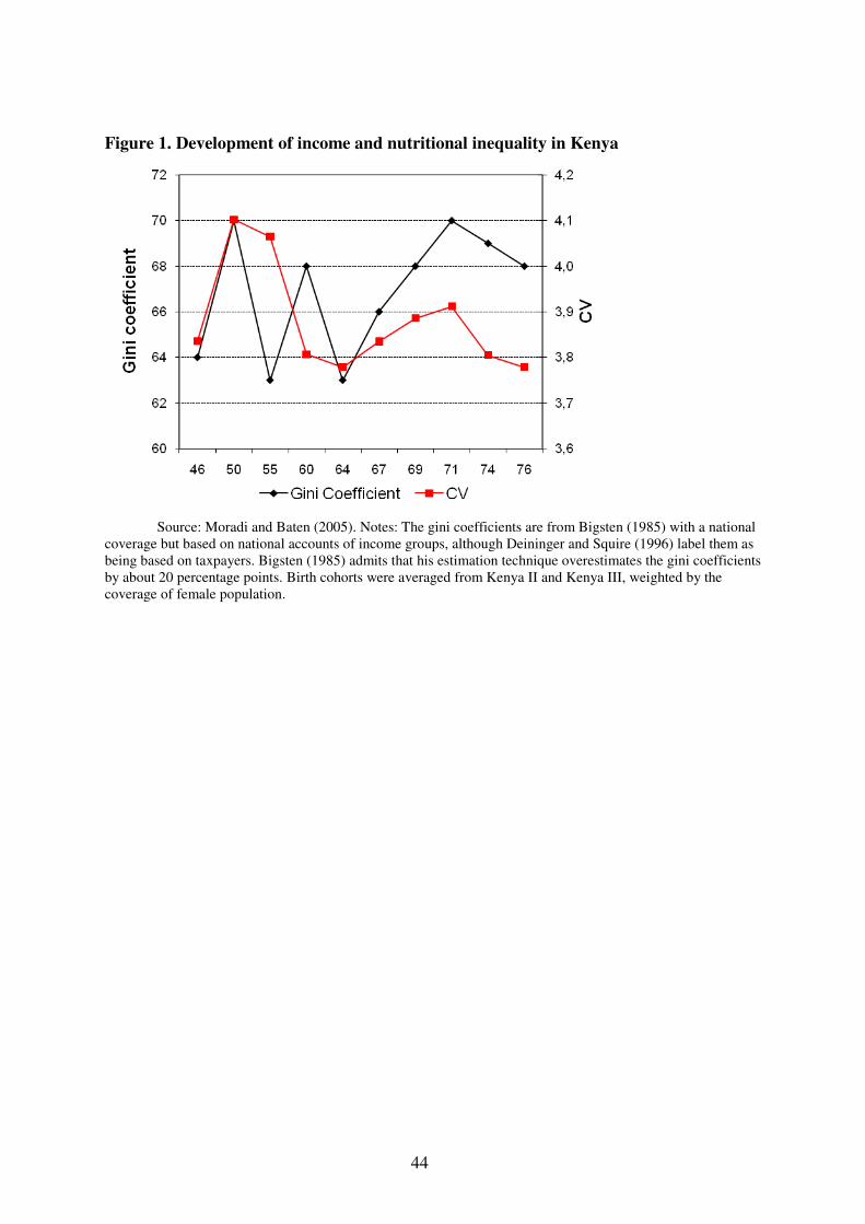
44
Figure 1. Development of income and nutritional inequality in Kenya
Source: Moradi and Baten (2005). Notes: The gini coefficients are from Bigsten (1985) with a national
coverage but based on national accounts of income groups, although Deininger and Squire (1996) label them as
being based on taxpayers. Bigsten (1985) admits that his estimation technique overestimates the gini coefficients
by about 20 percentage points. Birth cohorts were averaged from Kenya II and Kenya III, weighted by the
coverage of female population.
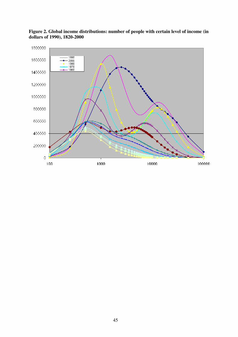
45
Figure 2. Global income distributions: number of people with certain level of income (in
dollars of 1990), 1820-2000
Related Documents