The CH abundance in turbulent, diffuse molecular clouds

MNRAS 453, 2747–2758 (2015) doi:10.1093/mnras/stv1782

The CH+ abundance in turbulent, diffuse molecular clouds

Andrew T. Myers,1‹ Christopher F. McKee2,3 and Pak Shing Li31Lawrence Berkeley National Laboratory, 1 Cyclotron Road, Berkeley, CA 94720, USA2Department of Physics, University of California, Berkeley, Berkeley, CA 94720, USA3Department of Astronomy, University of California, Berkeley, Berkeley, CA 94720, USA

Accepted 2015 August 3. Received 2015 July 30; in original form 2015 April 14

ABSTRACTThe intermittent dissipation of interstellar turbulence is an important energy source in thediffuse interstellar medium. Though on average smaller than the heating rates due to cosmicrays and the photoelectric effect on dust grains, the turbulent cascade can channel largeamounts of energy into a relatively small fraction of the gas that consequently undergoessignificant heating and chemical enrichment. In particular, this mechanism has been proposedas a solution to the long-standing problem of the high abundance of CH+ along diffusemolecular sight lines, which steady-state, low-temperature models underproduce by over anorder of magnitude. While much work has been done on the structure and chemistry of thesesmall-scale dissipation zones, comparatively little attention has been paid to relating thesezones to the properties of the large-scale turbulence. In this paper, we attempt to bridge thisgap by estimating the temperature and CH+ column density along diffuse molecular sightlines by post-processing three-dimensional magnetohydrodynamic(s) turbulence simulations.Assuming reasonable values for the cloud density (nH = 30 cm−3), size (L = 20 pc), andvelocity dispersion (σv = 2.3 km s−1), we find that our computed abundances compare wellwith CH+ column density observations, as well as with observations of emission lines fromrotationally excited H2 molecules.

Key words: astrochemistry – ISM: abundances – ISM: clouds.

1 IN T RO D U C T I O N

The CH+ ion is commonly detected along sight lines towards brightO and B stars, with column densities �1013 cm−2 frequently re-ported in the literature (e.g. Gredel, van Dishoeck & Black 1993;Crane, Lambert & Sheffer 1995; Gredel 1997; Sheffer et al. 2008;Weselak et al. 2008). This prevalence is puzzling, however, becauseCH+ is destroyed very efficiently by both atomic and molecularhydrogen, and the only reaction that can form CH+ rapidly,

C+ + H2 → CH+ + H �E/k = −4640 K, (1)

is strongly endothermic and can only proceed at temperatures of∼1000 K or higher. For this reason, models of diffuse interstellarclouds with T � 100 K, like those of van Dishoeck & Black (1986),fail dramatically to reproduce these high CH+ columns, despitetheir success with other species.

Most proposed solutions to this problem have invoked an ad-ditional energy source to overcome this 4640 K activation bar-rier. Possibilities include hydrodynamic (Elitzur & Watson 1978,1980) and magnetohydrodynamic (MHD; Draine & Katz 1986)

�E-mail: [email protected]

shock waves, heating in turbulent boundary layers at cloud surfaces(Duley et al. 1992), and particularly dense photon-dominatedregions (PDRs) surrounding bright stars (Duley et al. 1992;Sternberg & Dalgarno 1995); for an overview of these mechanismsand some of the problems they face confronting observations, seeGredel (1997). A particularly promising idea, pioneered by Fal-garone & Puget (1995), is that the intermittent dissipation of tur-bulence heats small regions within diffuse clouds to the �1000 Ktemperatures required for (1) to proceed. Drawing on laboratoryexperiments of unmagnetized, incompressible turbulent flows, theycalculated that if the velocity dispersion in cold, mostly atomicclouds at a scale of 1 pc is 3 km s−1, then a few per cent of the cloudcould be heated to >1000 K, a mass fraction sufficient to bring theCH+ abundance in line with observed values (Lambert & Danks1986). This result was later found to be consistent with magnetized,compressible turbulence simulations as well (Pan & Padoan 2009).These pockets of warm gas may also explain the observed emissionfrom the first few excited rotational states of H2 detected in diffusegas, which is often too large to be explained by UV pumping alone(e.g. Falgarone et al. 2005; Goldsmith et al. 2010; Ingalls et al.2011).

Models that rely on turbulent heating alone can overpredict theabundance of other species, such as OH, which is already well

C© 2015 The AuthorsPublished by Oxford University Press on behalf of the Royal Astronomical Society

Dow

nloaded from https://academ

ic.oup.com/m

nras/article/453/3/2747/1079846 by guest on 21 January 2022

mailto:[email protected]

2748 A. T. Myers, C. F. McKee and P. S. Li

modelled by cold cloud models (Federman et al. 1996). However,in addition to the direct heating effect, turbulence can give rise tonet drift velocities between the ionic and neutral species in plasmas,enhancing the rates of ion-neutral reactions like (1) beyond thoseexpected from the kinetic temperature alone (e.g. Draine 1980;Flower, Pineau des Forets & Hartquist 1985). Federman et al. (1996)approximated this effect by computing the rate of reaction (1) at theeffective temperature Teff given by

Teff = T + μ

3kv2

d, (2)

where μ is the reduced mass of (1) and vd is the magnitude ofthe ion-neutral drift velocity. They proposed that MHD waves withamplitudes ∼3 km s−1 can enhance the predicted column densitiesof CH+ to the observed values even in gas that remains T � 100 K.A similar calculation was made in Spaans (1995), who computedthe distribution of vd from an analytic intermittency model. Morerecently, Sheffer et al. (2008) included this effect in their PDRmodels, finding a similar result. The appeal of these models is thatthey have fewer problems overproducing molecules such as OH,which is not formed by an ion-neutral reaction.

The most successful models include both these effects simul-taneously. Joulain et al. (1998) and Godard, Falgarone & PineauDes Forets (2009) treat regions of intense dissipation, termed ‘tur-bulent dissipation regions (TDRs) by Godard et al., as magne-tized vortices, taking their (axisymmetric) velocity profiles fromthat of a Burgers vortex, for which the vorticity as a function ofradius is

ω(r) = ω0 exp

[−

(r

r0

)2]. (3)

Here, ω0 and r0 are parameters describing the peak vortic-ity and characteristic fall-off radius in the vortex. Typically,ω0 ≈ 6 × 10−10 s−1 and r0 ≈ 40 au in Godard et al. (2009). Thesecalculations follow the subsequent thermal and chemical evolutionof parcels of gas trapped inside such a vortex, including both turbu-lent heating and ion-neutral drift. Godard et al. (2009) then constructmodels of entire sight lines by assuming that they intersect somenumber of these vortex structures to account for the observed col-umn density of CH+. These models have had a great deal of successreproducing the observed CH+ and excited H2 columns withoutoverproducing species such as OH.

The goal of this paper is to provide a complementary approachto the above models, which concentrate on individual dissipationevents. We post-process the gas temperature T, drift velocity vd,and CH+ abundance cell by cell through an output of a turbulencesimulation from Li et al. (2012a) that has been scaled to typicaldiffuse cloud conditions. This approach loses some of the details ofthe above models, but it has the advantage of making fewer simpli-fying assumptions about, for example, the nature of the intermittentstructures or the number of dissipation events along a line of sight.We find that CH+ columns in excess of ∼1013 cm−2 are readily ob-tained. We compare our results against a statistically homogenoussample of CH+-containing sight lines from Weselak et al. (2008)and against observations of rotationally excited H2, finding goodagreement with both.

2 M E T H O D O L O G Y

In this section, we provide an overview of our calculation, includingour treatment of the heating and cooling rates, the drift velocity, andour calculation of the CH+ abundance.

2.1 Model description

The CH+ ion is believed to form in partially molecular environ-ments. Indeed, in order for reaction (1) to proceed, at least someof the hydrogen must be in the form of H2, and at least some ofthe carbon must be in C+. Any plausible formation mechanism isthus not likely to be effective in either the outskirts of molecularclouds with visual extinction AV < 0.1 mag, where the hydrogenis almost all atomic, or deep in their interiors at AV greater than afew, where almost all the carbon will be C and/or CO. This gas issometimes referred to as the ‘dark gas since it is difficult to observe(Grenier, Casandjian & Terrier 2005; Wolfire, Hollenbach & McKee2010).

We therefore model interstellar clouds in which hydrogen hasbegun to turn to H2, but carbon is still primarily in the form of C+.Snow & McCall (2006) classify such clouds as ‘diffuse molecu-lar clouds. We treat these regions as cubic boxes with length �0,mean hydrogen nucleus number density nH, and one-dimensionalvelocity dispersion σ 1D. The mean mass per hydrogen nucleus isμH = 2.34 × 10−24 g cm−3. For simplicity, we set the relative abun-dances (relative to hydrogen nuclei) of molecular hydrogen x(H2)and ionized carbon x(C+) to be constant across the region. For theformer, we adopt x(H2) = 0.16, the mean observed molecular frac-tion from the sample of Weselak et al. (2008), which studied thecorrelation of CH+ column density with that of atomic and molecu-lar hydrogen. For the latter, we take x(C+) = 1.6 × 10−4 from Sofiaet al. (2004). Sofia et al. (2011) find using a different measurementtechnique that the gas-phase carbon abundance is lower than thatadopted here by a factor of ≈0.43. Since it is not clear which mea-surement is more accurate, we choose to adopt the higher value. Theeffects of a lower C abundance in our model are complex. On onehand, it directly reduces the CH+ formation rate (see Section 2.5),since C+ is one of the reactants in (1). On the other hand, it decreasesthe cooling rate due to C+ (Section 2.3) and increases our estimatefor the ion-neutral drift velocity (Section 2.4). The overall effectof deceasing our assumed carbon abundance by a factor of 0.43 isto increase the estimate for the CH+ abundance by approximately30 per cent.

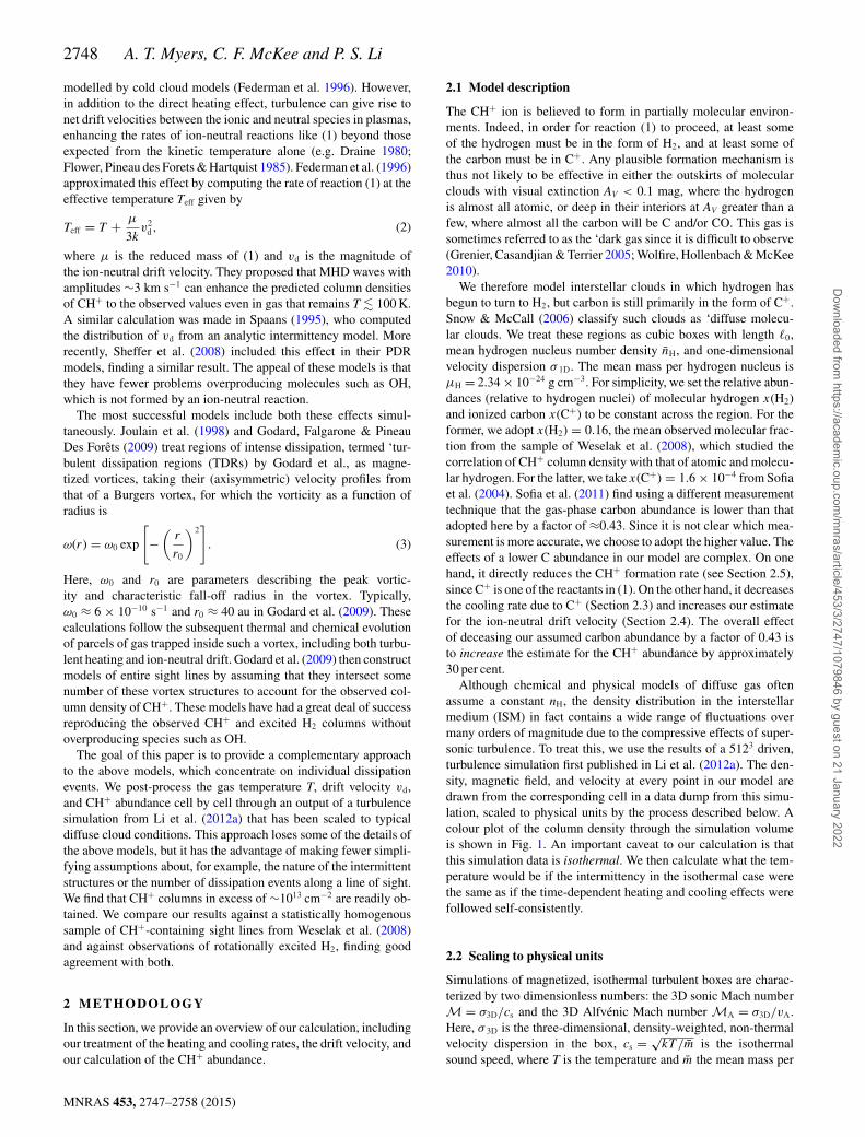
Although chemical and physical models of diffuse gas oftenassume a constant nH, the density distribution in the interstellarmedium (ISM) in fact contains a wide range of fluctuations overmany orders of magnitude due to the compressive effects of super-sonic turbulence. To treat this, we use the results of a 5123 driven,turbulence simulation first published in Li et al. (2012a). The den-sity, magnetic field, and velocity at every point in our model aredrawn from the corresponding cell in a data dump from this simu-lation, scaled to physical units by the process described below. Acolour plot of the column density through the simulation volumeis shown in Fig. 1. An important caveat to our calculation is thatthis simulation data is isothermal. We then calculate what the tem-perature would be if the intermittency in the isothermal case werethe same as if the time-dependent heating and cooling effects werefollowed self-consistently.

2.2 Scaling to physical units

Simulations of magnetized, isothermal turbulent boxes are charac-terized by two dimensionless numbers: the 3D sonic Mach numberM = σ3D/cs and the 3D Alfvenic Mach number MA = σ3D/vA.Here, σ 3D is the three-dimensional, density-weighted, non-thermalvelocity dispersion in the box, cs = √

kT /m is the isothermalsound speed, where T is the temperature and m the mean mass per

MNRAS 453, 2747–2758 (2015)

Dow


ic.oup.com/m


CH+ in diffuse molecular clouds 2749

Figure 1. Logarithm of the total column density NH through the computational domain along the x direction. The simulation data has been scaled such thatthe mean NH is 1.83 × 1021 cm−2. The size of the box is indicated on the x and y axes.

particle, and vA = Brms/√

4πρ is the Alfven velocity, where Brms

is the root-mean-square magnetic field and ρ the mean density. Inthe simulation considered here, the turbulence was driven so as tomaintain M ≈ 10, and the initial MA was

√5.

In the absence of further constraints, we would be free to scaleρ, σ 3D, cs, Brms, and the size of the box �0 at will as long as thedimensionless ratios M and MA remained invariant (see McKee,Li & Klein 2010 for a more rigorous discussion of scaling laws forturbulent box simulations). However, to be consistent with obser-vations of diffuse molecular gas, we impose several additional con-straints. First, we require that the gas in the box obey a linewidth-sizerelation (e.g. McKee & Ostriker 2007):

σ1D = σpcR0.5pc , (4)

where Rpc is the cloud radius in parsecs, and σ pc = 0.72 km s−1. The1D non-thermal velocity dispersion σ 1D is related to the 3D valueby σ3D = √

3σ1D, and in applying equation (4), which is meant forapproximately spherical clouds, to our cubic simulation domain, weidentify the cloud radius R with �0/2. Secondly, we require that themean column density of hydrogen nuclei be fixed:

NH = nH�0 = Nobs, (5)

where Nobs ≈ 1.83 × 1021 cm−2 is the mean total column densityfrom Weselak et al. (2008). This column corresponds to AV ≈ 1,consistent with our requirement that the gas be partially molecular.Note that equations (4) and (5) imply that we cannot indepen-dently choose nH, �0, and σ 1D; choosing a density fixes the box size�0, which fixes the velocity dispersion through the linewidth-size

relation. Numerically:

�0 ≈ 19.8(

30 cm−3

nH

)pc,

σ1D ≈ 2.3(

30 cm−3

nH

)0.5km s−1 . (6)

The dynamical time-scale in our model can thus be estimated as

tdyn = �0

σ1D≈ 8.5 × 106

(30 cm−3

nH

)0.5

yr. (7)

We assume that properties of the fluid flow (the density, velocity,and magnetic field) change on this time-scale. We show that this islarge compared to the thermal and chemical time-scales below.

These relations also fix (along with the fact the MA = 2.2) therms magnetic field strength in the box:

Brms =√

6πμHNobsσ 2pc

(1 pc) M2A

≈ 5.3 μG. (8)

Crutcher et al. (2010) infer that interstellar fields in gas with nH �300 cm−3 are uniformly distributed in strength between very lowvalues and 10 μG, so this field is quite typical. Note that only oneof nH, �0, σ 3D, and Brms may be set independently, with the othersfollowing from that choice.

The final remaining dimensional parameter describing our turbu-lence simulation is the isothermal sound speed cs. The sound speedof a gas with x(H2) = 0.16 and x(He) = 0.1 is

cs(T ) ≈ 0.74

√T

100 Kkm s−1. (9)

MNRAS 453, 2747–2758 (2015)

Dow


ic.oup.com/m



Table 1. Standard physical andchemical model parameters.

nH 30 cm−3

L 20 pcσ 1D 2.3 km s−1

TM 65 KT50,M 35 KBrms 5.2 µGx(H) 0.68x(H2) 0.16x(He) 0.1x(e−) 1.6 × 10−4

x(C) 1.6 × 10−4

x(O) 3.2 × 10−4

However, because the temperature is an output of our model, wecannot set it arbitrarily. We thus compute the temperature usingthe process described below for a range of boxes, each scaled toa different nH, and select the one for which M computed usingthe mass-weighted median temperature T50,M (the T for which halfof the mass in cloud is hotter) is ≈10. We find that this occurs atnH ≈ 30 cm−3 and adopt that as our fiducial density. This is thesame value adopted in the standard model of Joulain et al. (1998).However, individual sight lines passing through the simulation vol-ume can have mean densities ranging from ≈5 to ≈180 cm−3. Thecorresponding T50,M is ≈35 K, and the mass-weighted mean tem-perature is TM ≈ 65 K. We summarize the physical and chemicalparameters describing this model in Table 1.

Our simulation data does not include the effects of self-gravity.As a consistency check, we compute the virial parameter αvir toverify that turbulence indeed dominates self-gravity. Using theabove parameters, the total mass M in the box is ≈8000 M�.The virial parameter for a spherical cloud of mass M and radius Ris αvir = 5σ 2

1DR/GM (Bertoldi & McKee 1992). Using R = �0/2,we find αvir ≈ 7.4, which is large enough that the effects of self-gravity are indeed negligible. We can also characterize the relativeimportance of gravity and magnetic fields in the box by comput-ing the mass-to-flux ratio relative to critical, μ ≡ M/M, whereM ≈ /2π

√G and is the magnetic flux threading the cloud.

For our adopted parameters, μ ≈ 1.3, so the cloud is marginallymagnetically supercritical.

2.3 Heating and cooling

The temperature in each cell is set by a balance between heatingand cooling:

Turb + CR + PE = nH�tot(T ), (10)

where Turb, CR, and PE are the heating rates per unit volumedue to the dissipation of turbulence, cosmic ray ionizations, andthe photoelectric effect on dust grains, respectively. nH�tot(T) is thetotal cooling rate per unit volume, which we assume is dominated byelectronic transitions of C+ and O and by rovibrational transitionsof the H2 molecule. Note that throughout this paper, we use λ torepresent the cooling rate coefficient (erg cm3 s−1) and � for thecooling rate per H nucleus (erg s−1).

CR can be expressed as the product of three factors – the totalcosmic ray ionization rate per H nucleus ζ H (including both primaryand secondary ionizations), the average energy deposited into themedium per ionization �Q, and nH. Both ζ H and �Q are ratheruncertain and can vary considerably over different Galactic envi-ronments. Typical values of ζ H in dense gas are ∼1–5 × 10−17 s−1

(Dalgarno 2006), but there is evidence from H3+ observations that

ζ H is considerably higher in the diffuse gas under considerationhere (Dalgarno 2006; Indriolo & McCall 2012). Indriolo & McCall(2012) find a mean ζ H of 1.8 × 10−16 s−1 in their sample of diffusemolecular sight lines, and values as large as ∼1 × 10−15 s−1 havebeen reported in the literature (Snow & McCall 2006; Shaw et al.2008). In this paper, we adopt the value 1.8 × 10−16 s−1. For �Q,we use 10 eV, as estimated for diffuse molecular gas from table 6of Glassgold, Galli & Padovani (2012), although it is important tonote that this value can vary by several eV depending on the precisephysical and chemical conditions in the cloud. Combining thesefactors, the cosmic ray heating rate is

CR = ζ�QnH

≈ 1.9 × 10−25( nH

30 cm−3

)ergs cm−3 s−1. (11)

For PE, we adopt the expression:

PE = 1.3 × 10−24 nHεG0 ergs cm−3 s−1 (12)

from Wolfire et al. (2003), where G0 is the intensity of FUV light inunits of the Habing (1968) field and ε is the heating efficiency factorgiven by equation 20 of Wolfire et al. (2003). For nH = 30 cm−3,T = 100 K, an electron fraction of 1.6 × 10−4, and a FUV fieldof G0 = 1.1 (Mathis, Mezger & Panagia 1983), ε evaluates to1.8 × 10−2, yielding

PE = 7.6 × 10−25( nH

30 cm−3

)ergs cm−3 s−1. (13)

The final heating process we consider is Turb. Dimensional ar-guments (e.g. Landau & Lifshitz 1959) and numerical simulations(e.g. Stone, Ostriker & Gammie 1998; Mac Low 1999) both sug-gest that the kinetic energy in a turbulent cloud 1/2ρσ 2

3D decaysin roughly one crossing time �0/σ3D, so that the volume-averagedturbulent heating rate is approximately

Turb ≈ 1

2

ρσ 33D

�0

≈ 3.5 × 10−26

√nH

30 cm−3ergs cm−3 s−1, (14)

where in the last step we have assumed the scaling given by equa-tions (4) and (5). Locally, however, Turb exhibits large fluctuationsfrom place to place, a phenomenon known as intermittency. To cal-culate the spatial dependence of Turb, we follow the calculationin Pan & Padoan (2009). To summarize their argument, the workdone against the viscous forces in a fluid with velocity field v isirreversibly converted into heat at rate per unit volume given by

Turb(x) = 1

2ρν

(∂ivj + ∂j vi − 2

3(∇ · v) δij

)2

. (15)

This rate depends on the kinematic viscosity of the fluid, ν. However,in our simulations, which were based on the Euler equations for acompressible gas, the viscosity was numerical in origin, and thusdoes not have its true microphysical value. Instead, we treat ν as aproportionality constant that takes whatever value is required so thatthe volume average of equation (15) equals equation (14). Once thisconstant has been determined, we can compute Turb(x) for eachcell in the simulation.

Note that the resolution of our simulation data�x = �0/512 ≈ 8 × 103 au is significantly larger than thedissipation scale provided by the kinematic viscosity of interstellargas of �d ∼ 10 au (Joulain et al. 1998). If the turbulence wereallowed to cascade down to these small scales, the distribution

MNRAS 453, 2747–2758 (2015)

Dow


ic.oup.com/m



of the heating rate would be more intermittent than it is in oursimulation (Pan & Padoan 2009). However, viscous dissipationis not the only process that removes energy from the turbulentcascade. Ion-neutral friction becomes significant at the muchlarger scale �AD (see Section 2.4), and is capable of dissipatingmost (≈70 per cent for MA ≈ 1) of the energy in the cascade atscales ≈ 10 �AD (Li, Myers & McKee 2012b), which is comparableto the cell size in our numerical data. Below �AD, a turbulentcascade can reassert itself in the neutrals, allowing some of theenergy to be dissipated on the ∼10 au scale set by viscosity. Whileour procedure likely underestimates the intermittency for thisremaining ≈30 per cent of the energy, it is more accurate than theopposite assumption that all the energy in cascade makes it to∼10 au scales. Note that this procedure for estimating the turbulentheating rate is scaled such that it includes all the energy removedfrom the turbulent cascade by dissipative processes, whether thephysical mechanism is molecular viscosity or ambipolar diffusion.We do not separately include an ambipolar diffusion heating term inequation (10) because doing so would amount to double counting.

For the C+ and O cooling coefficients, we adopt the formulasgiven by Wolfire et al. (2003):

λC+ (T ) = 3.6 × 10−27 exp (−92 K/T ) erg cm3 s−1

λO(T ) = 2.35 × 10−27

(T

100 K

)0.4

× exp (−228 K/T ) erg cm3 s−1, (16)

where we have scaled the overall numerical factors to account forour fractional abundances of carbon and oxygen of 1.6 × 10−4 and3.2 × 10−4, respectively, rather than the 1.4 × 10−4 and 3.4 × 10−4

used in Wolfire et al. (2003). The cooling rates per H nucleus arethen �C+ (T ) = nHλC+ (T ) and �O(T) = nHλO(T). These rates arevalid for nH < ncrit 3000 cm−3.

The final thermal process we consider is the cooling rate due tothe H2 molecule. This coolant is particularly important in the warm(over a few hundred K) gas in which CH+ is expected to form.In the low-density limit, the H2 level populations are subthermaland the cooling rate �H2 (nH → 0)(T ) is a sum over the rates dueto collisions with H, H2, He, and e. For these rates, we use thetables in Glover & Abel (2008), assuming an ortho:para ratio of0.7 (see Section 3.3) and the fractional abundances of H, H2, He,and electrons listed in Table 1. These rates are valid at arbitrarilylow gas densities, since the cooling rate coefficients themselvesare independent of the gas density in this limit. At densities highenough for local thermodynamic equilibrium to be established, theH2 cooling rate per H nucleus �H2, LTE(T ) becomes independentof the collision partner abundances, and we adopt the cooling ratefrom Coppola et al. (2012). We bridge these two limits followingHollenbach & McKee (1979):

�H2 (T ) = �H2, LTE(T )

1 + �H2, LTE(T )/�H2 (nH → 0)(T )(17)

The total cooling rate is then

�tot(T ) = �C+ (T ) + �O(T ) + xH2�H2 (T ). (18)

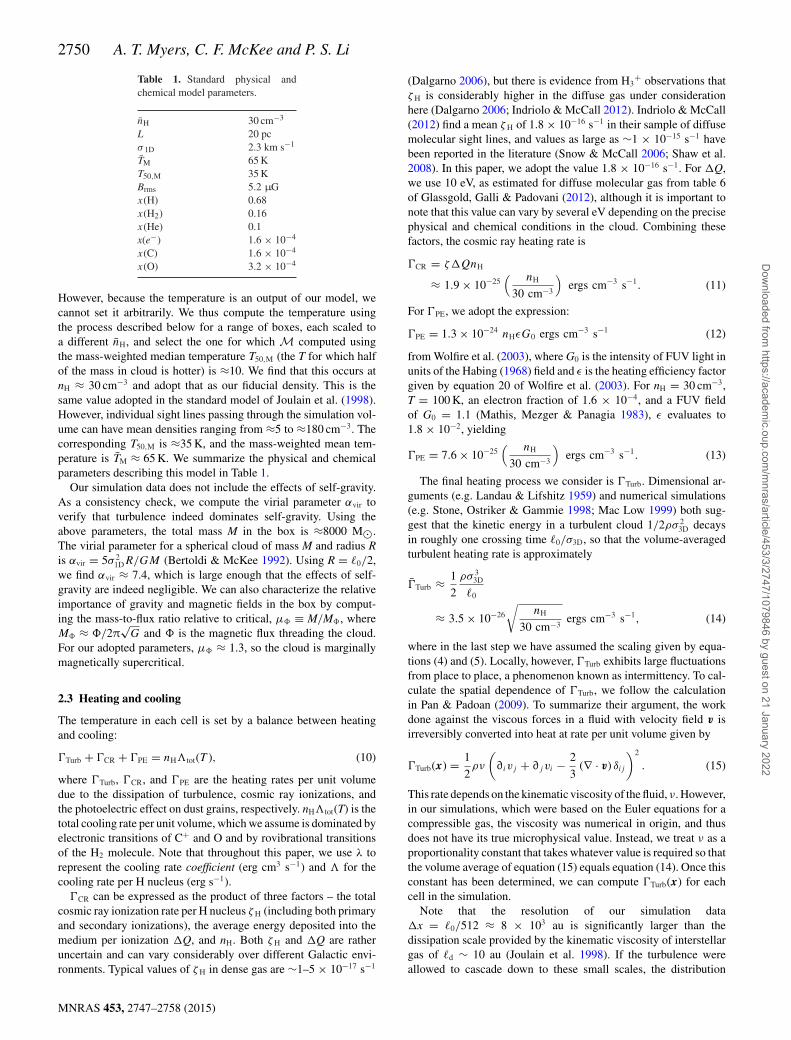
Equation (10) becomes a non-linear equation for Tin each cell, which we solve numerically using thescipy.optimize.brenth routine from the SCIPY soft-ware library (Jones et al. 2001). The magnitudes of these coolingprocesses are summarized as a function of temperature in Fig. 2for our standard model parameters. For comparison, the (constant)

Figure 2. Heating (red) and cooling (blue) rates per unit volume versusT for nH = 30 cm−3 and the standard chemical abundances are shown inTable 1. The solid blue curve shows nH�tot, while the dashed, dashed-dotted,and dotted curves are nH�H2 , nH�C+ , and nH�O, respectively. The solid,dashed, and dashed-dotted red lines show the mean values of Turb, PE,and CR, respectively.

values of various heating rates are also displayed for our standarddensity of nH = 30 cm−3.

We estimate the typical cooling time in our model as the thermalenergy density divided by the cooling rate:

tcool = 3/2kT

�tot(T ) 3.3 × 104yr, (19)

where the numerical evaluation is for our fiducial values ofnH = 30 cm−3 and T50,M = 35 K. This is two orders of magnitudesmaller than the dynamical time (equation 7), which justifies ouruse of an energy balance equation.

2.4 Ion-neutral drift

In the presence of ambipolar diffusion (the net slippage betweenthe charged and neutral species in a plasma), ion-neutral reactionslike (1) can proceed at rates faster than those expected from thekinetic temperature alone (e.g. Draine 1980; Flower et al. 1985).The relative importance of the ambipolar and inertial forces in aturbulent system can be characterized by the ambipolar diffusionReynolds number RAD(�0) (Zweibel & Brandenburg 1997; Li et al.2012b):

RAD(�0) ≡ 4πγADρiρn�0σ3D

B2rms

, (20)

where ρ i and ρn are the densities of the ionic and neutral com-ponents of the fluid and γ AD is the ion-neutral coupling con-stant given by 〈σv〉/(mi + mn). For C+ and H2, this evaluates to8.47 × 1013 cm3 s−1 g−1 (Draine 1980). Applying equations (4) and(5) for our adopted degree of ionization and magnetic field strength,RAD(�0) is

RAD(�0) ≈ 6.3 × 103

√( nH

30 cm−3

) 1. (21)

The corresponding length-scale �AD = �0/RAD(�0) at which ambipo-lar dissipation becomes significant is ≈640 au for nH = 30 cm−3.Thus, ambipolar drift should not be significant on large scales in ourmodel. However, as with the turbulent heating rate, there may beisolated regions in the tails of the drift velocity distribution wherethis effect is significant.

MNRAS 453, 2747–2758 (2015)

Dow


ic.oup.com/m



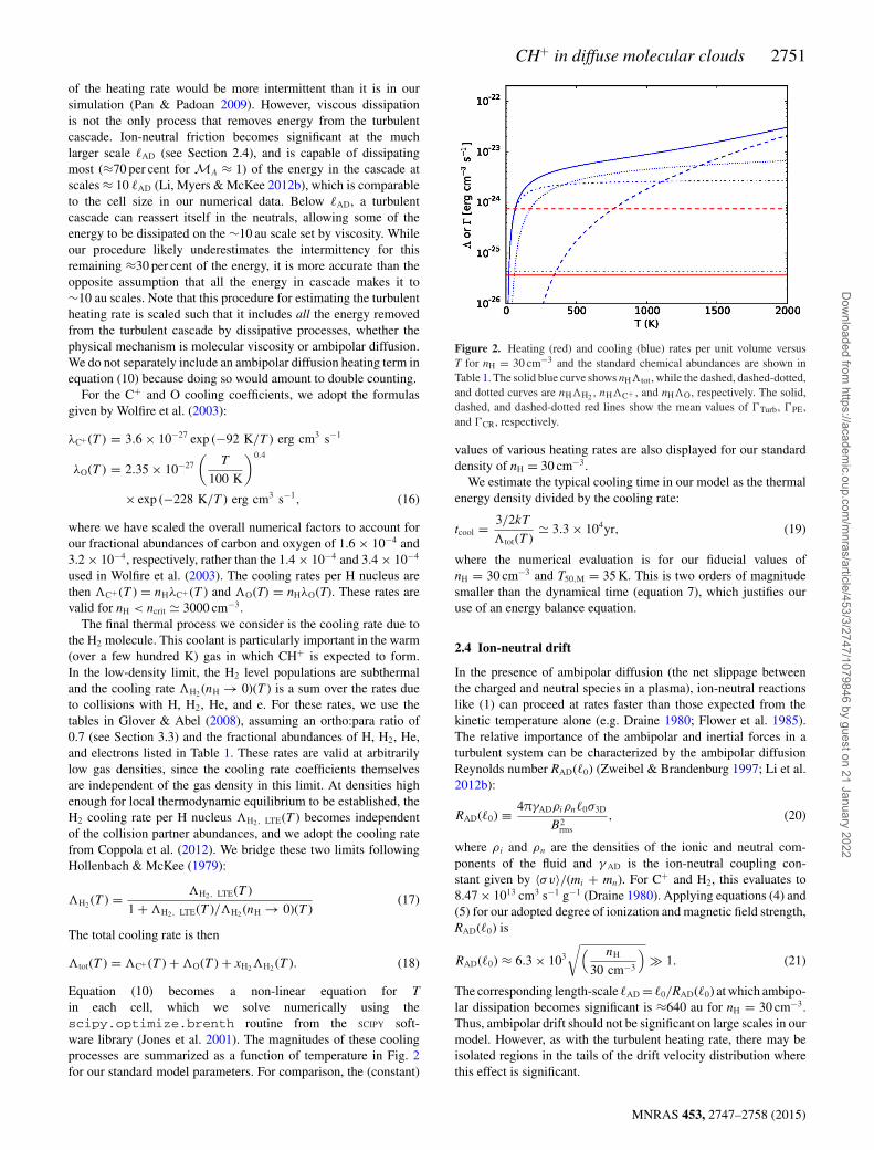
Figure 3. Blue – the circles show the mass-weighted distribution of vd di-vided by its mean value 〈vd〉 from theM = 3,MA = 0.67, RAD(�0) ≈ 1000AD simulation. The error bars show the 2σ temporal variation in distributionover two box crossing times, and solid line shows the best-fitting lognormal.Green – same, but for the M = 3, MA = 0.67 ideal simulation, with vd

computed from equation (22). The agreement between the two curves isquite good over more than three standard deviations.

To proceed, we need a prescription for computing vd. Unfortu-nately, two-fluid simulations of MHD turbulence are prohibitivelyexpensive in the high M, strongly coupled regime considered here.To estimate the effects of vd on the production of CH+, we insteaduse our ideal MHD data along with an approximate analytic ex-pression for the drift velocity in the strongly coupled regime, whichwe corroborate with direct numerical simulations of turbulent am-bipolar diffusion at lower M. Specifically, if the system is weaklyionized, then the Lorentz force and the ion-neutral drag force dom-inate all the other terms in the ion momentum equation and thedrift is given by vd = |(∇ × B) × B|/4πγADρiρn (e.g. Shu 1992).If the effects of ambipolar diffusion are weak enough that they haveonly a minor effect on the geometry of the magnetic field, we canestimate the drift by computing |(∇ × B) × B| in the ideal limit:

vd ≈ |∇ × B × B|Ideal

4πγADρiρn

. (22)

This procedure is illustrated in Fig. 3. We take two simulationsof M = 3, MA = 0.67 turbulence from Li et al. (2008), one whichfollows the ion and neutral fluids separately, and one which as-sumes ideal MHD. The AD simulation has RAD(�0) ≈ 1000. Wedirectly compute the time-averaged, density-weighted distributionof vd in the non-ideal simulation, and compare it to that of equa-tion (22) computed using the ideal data with γ AD and χ i chosen tomatch the AD simulation. The resulting distributions both have anapproximately lognormal form:

P (log vd)d log vd =1

σlog vd

√2π

exp

(− (log vd − μlog vd )2

2σ 2log vd

)(23)

and agree with each other to within the error bars, which showthe magnitude of the temporal fluctuation in the drift distributioncomputed over two crossing times. Equation (22) does slightly over-predict the simulated value of vd: both the mean μlog vd and standarddeviation σlog vd of the Lorentz drift approximation are larger thanthose of the lognormal fit to the true drift distribution by 5 and2 per cent, respectively. This is likely because, although RAD(�0) for

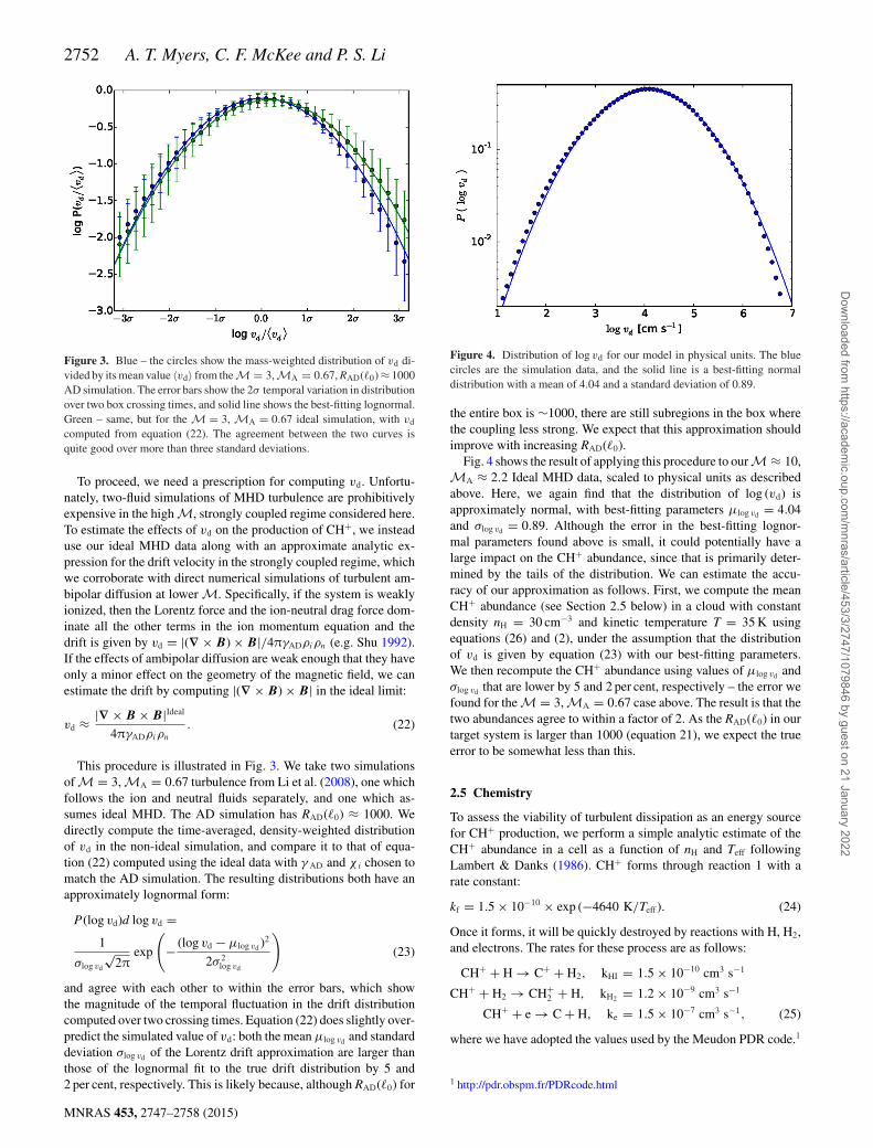
Figure 4. Distribution of log vd for our model in physical units. The bluecircles are the simulation data, and the solid line is a best-fitting normaldistribution with a mean of 4.04 and a standard deviation of 0.89.

the entire box is ∼1000, there are still subregions in the box wherethe coupling less strong. We expect that this approximation shouldimprove with increasing RAD(�0).

Fig. 4 shows the result of applying this procedure to ourM ≈ 10,MA ≈ 2.2 Ideal MHD data, scaled to physical units as describedabove. Here, we again find that the distribution of log (vd) isapproximately normal, with best-fitting parameters μlog vd = 4.04and σlog vd = 0.89. Although the error in the best-fitting lognor-mal parameters found above is small, it could potentially have alarge impact on the CH+ abundance, since that is primarily deter-mined by the tails of the distribution. We can estimate the accu-racy of our approximation as follows. First, we compute the meanCH+ abundance (see Section 2.5 below) in a cloud with constantdensity nH = 30 cm−3 and kinetic temperature T = 35 K usingequations (26) and (2), under the assumption that the distributionof vd is given by equation (23) with our best-fitting parameters.We then recompute the CH+ abundance using values of μlog vd andσlog vd that are lower by 5 and 2 per cent, respectively – the error wefound for the M = 3, MA = 0.67 case above. The result is that thetwo abundances agree to within a factor of 2. As the RAD(�0) in ourtarget system is larger than 1000 (equation 21), we expect the trueerror to be somewhat less than this.

2.5 Chemistry

To assess the viability of turbulent dissipation as an energy sourcefor CH+ production, we perform a simple analytic estimate of theCH+ abundance in a cell as a function of nH and Teff followingLambert & Danks (1986). CH+ forms through reaction 1 with arate constant:

kf = 1.5 × 10−10 × exp (−4640 K/Teff ). (24)

Once it forms, it will be quickly destroyed by reactions with H, H2,and electrons. The rates for these process are as follows:

CH+ + H → C+ + H2, kHI = 1.5 × 10−10 cm3 s−1

CH+ + H2 → CH+2 + H, kH2 = 1.2 × 10−9 cm3 s−1

CH+ + e → C + H, ke = 1.5 × 10−7 cm3 s−1, (25)

where we have adopted the values used by the Meudon PDR code.1

1 http://pdr.obspm.fr/PDRcode.html

MNRAS 453, 2747–2758 (2015)

Dow


ic.oup.com/m


http://pdr.obspm.fr/PDRcode.html


Because the electron fraction xe ≈ xi is ∼10−4, removal of CH+

by electrons is not crucial and we ignore it in our calculations.However, destruction by atomic and molecular hydrogen are bothimportant. Balancing the rate of formation with the rate of destruc-tion nC+nH2kf = nCH+nHIkHI + nCH+nH2kH2 , we can derive

nCH+ = x(C+)x(H2)

1 − 2x(H2)

kf

kHI

(1 + kH2

kHI

x(H2)

1 − 2x(H2)

)−1

nH

≈ 3.9 × 10−4( nH

30 cm−3

)× exp

(−4640 K

Teff

). (26)

Equation (26) highlights the importance of both the molecular frac-tion and the C+ abundance for CH+ production; the gas must bewell shielded enough from the ambient radiation field that some ofthe hydrogen is molecular form, but not so well shielded that carbonis all molecular.

We can also estimate a typical CH+ formation time-scale asfollows. Suppose we are in a region that initially contains no CH+

that is subsequently subject to heating. From reaction 25, the rateof change in nCH+ is

dnCH+

dt= nC+nH2kf − nCH+nHIkHI − nCH+nH2kH2 . (27)

The solution to this equation is

nCH+ (t) = nCH+,eq × [1 − exp (−at)

], (28)

where nCH+,eq is the equilibrium abundance given by equation (26)and a = (1 − 2xH2 )kHI + xH2kH2 . Thus, the time over which theCH+ abundance achieves 90 per cent of its equilibrium value is

tCH+ = ln(10)

a≈ 250 yr. (29)

This is two orders of magnitude shorter than the cooling time (equa-tion 19), and four orders shorter than the characteristic dynamicaltime (equation 7).

3 R ESULTS

3.1 Temperature and CH+ abundance

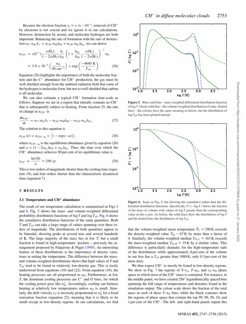
The result of our temperature calculation is summarized in Figs 5and 6. Fig. 5 shows the mass- and volume-weighted differentialprobability distribution functions of log T and log Teff. Fig. 6 showsthe cumulative distribution functions of the same quantities. BothT and Teff can take a large range of values spanning over three or-ders of magnitude. The distributions of both quantities appear tobe bimodal, showing peaks at several tens and several hundredsof K. The large majority of the mass lies at low T, but a smallfraction is found in high-temperature ‘pockets – precisely the ar-rangement proposed by Falgarone & Puget (1995). An interestingfeature of these distributions is the importance of density varia-tions in setting the temperature. The difference between the mass-and volume-weighted distributions shows that high values of T andTeff tend to be found in relatively low-density gas. This is easilyunderstood from equations (10) and (22). From equation (10), theheating processes are all proportional to nH. Furthermore, at lowT, the dominant cooling processes are C+ and O lines, for whichthe cooling power goes like n2

H. Accordingly, cooling can balanceheating at relatively low temperatures unless nH is small. Simi-larly, the drift velocity vd is inversely proportional to n2

H for a fixedionization fraction (equation 22), meaning that it is likely to besmall except in low-density regions. In our calculations, we find

Figure 5. Blue solid line – mass-weighted differential distribution functionof log T. Green solid line – the volume-weighted distribution of same. Dottedlines – the colours have the same meaning as before, but the distribution oflog Teff has been plotted instead.

Figure 6. Same as Fig. 5, but showing the cumulative rather than the dif-ferential distribution functions. Specifically, P (> log T ) shows the fractionof the mass or volume with values of log T greater than the correspondingvalue on the x-axis. As before, the solid lines show the distribution of log Tand the dotted lines the distribution of log Teff.

that the volume-weighted mean temperature TV ≈ 290 K exceedsthe density-weighted value TM ∼ 67 K by more than a factor of4. Similarly, the volume-weighted median T50,V ≈ 163 K exceedsthe mass-weighted median T50,M ≈ 35 K by a similar value. Thisdifference is particularly dramatic for the high-temperature tailsof the distribution: while approximately 8 per cent of the volumein our box has a Teff greater than 1000 K, only 0.3 per cent of themass does.

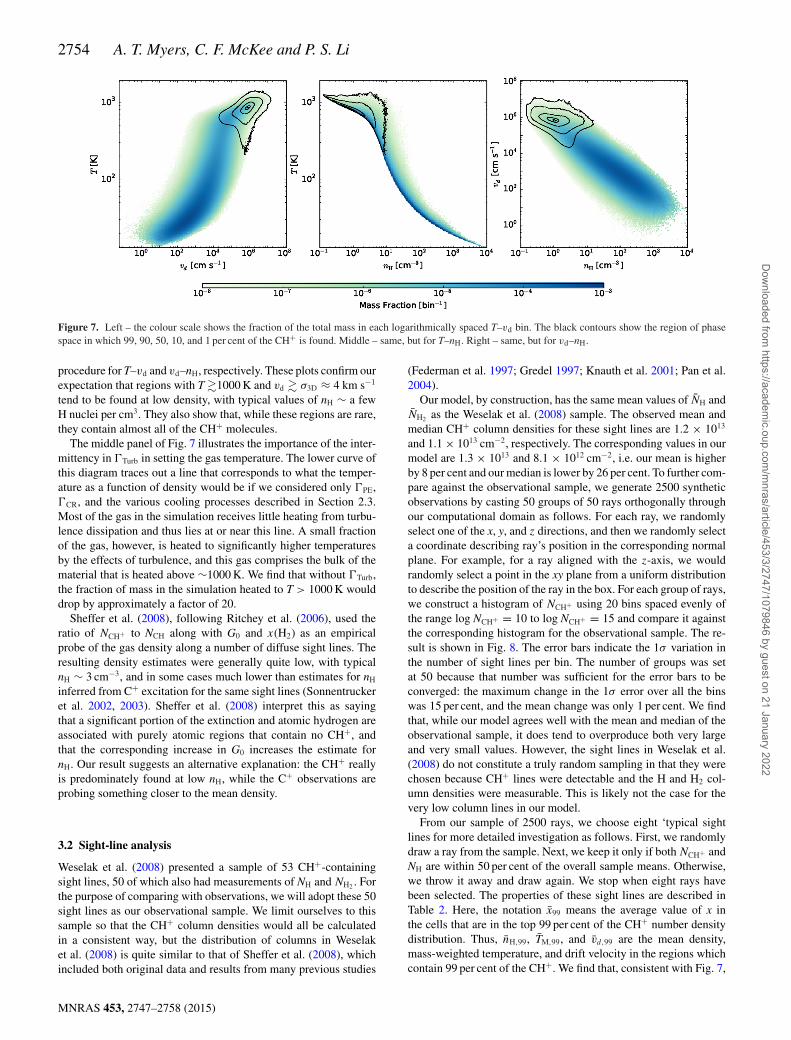
We thus expect CH+ to mostly be found in low-density regions.We show in Fig. 7 the regions of T–vd, T–nH, and vd–nH phasespace in which most of the CH+ mass is contained. For instance, inthe middle panel, we have created 2562 logarithmically spaced binsspanning the full range of temperatures and densities found in thesimulation output. The colour scale shows the fraction of the totalmass in each of these T–nH bins, while the black contours showthe regions of phase space that contain the top 99, 90, 50, 10, and1 per cent of the CH+. The left- and right-hand panels repeat this

MNRAS 453, 2747–2758 (2015)

Dow


ic.oup.com/m



Figure 7. Left – the colour scale shows the fraction of the total mass in each logarithmically spaced T–vd bin. The black contours show the region of phasespace in which 99, 90, 50, 10, and 1 per cent of the CH+ is found. Middle – same, but for T–nH. Right – same, but for vd–nH.

procedure for T–vd and vd–nH, respectively. These plots confirm ourexpectation that regions with T �1000 K and vd � σ3D ≈ 4 km s−1

tend to be found at low density, with typical values of nH ∼ a fewH nuclei per cm3. They also show that, while these regions are rare,they contain almost all of the CH+ molecules.

The middle panel of Fig. 7 illustrates the importance of the inter-mittency in Turb in setting the gas temperature. The lower curve ofthis diagram traces out a line that corresponds to what the temper-ature as a function of density would be if we considered only PE,CR, and the various cooling processes described in Section 2.3.Most of the gas in the simulation receives little heating from turbu-lence dissipation and thus lies at or near this line. A small fractionof the gas, however, is heated to significantly higher temperaturesby the effects of turbulence, and this gas comprises the bulk of thematerial that is heated above ∼1000 K. We find that without Turb,the fraction of mass in the simulation heated to T > 1000 K woulddrop by approximately a factor of 20.

Sheffer et al. (2008), following Ritchey et al. (2006), used theratio of NCH+ to NCH along with G0 and x(H2) as an empiricalprobe of the gas density along a number of diffuse sight lines. Theresulting density estimates were generally quite low, with typicalnH ∼ 3 cm−3, and in some cases much lower than estimates for nH

inferred from C+ excitation for the same sight lines (Sonnentruckeret al. 2002, 2003). Sheffer et al. (2008) interpret this as sayingthat a significant portion of the extinction and atomic hydrogen areassociated with purely atomic regions that contain no CH+, andthat the corresponding increase in G0 increases the estimate fornH. Our result suggests an alternative explanation: the CH+ reallyis predominately found at low nH, while the C+ observations areprobing something closer to the mean density.

3.2 Sight-line analysis

Weselak et al. (2008) presented a sample of 53 CH+-containingsight lines, 50 of which also had measurements of NH and NH2 . Forthe purpose of comparing with observations, we will adopt these 50sight lines as our observational sample. We limit ourselves to thissample so that the CH+ column densities would all be calculatedin a consistent way, but the distribution of columns in Weselaket al. (2008) is quite similar to that of Sheffer et al. (2008), whichincluded both original data and results from many previous studies

(Federman et al. 1997; Gredel 1997; Knauth et al. 2001; Pan et al.2004).

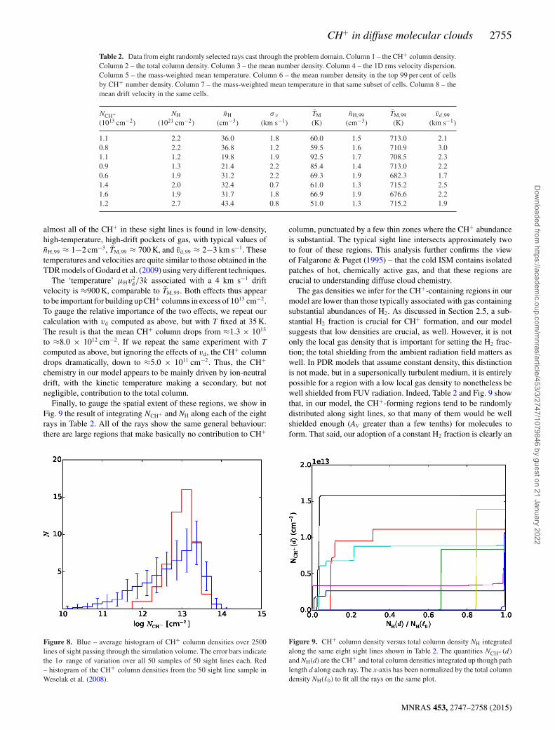
Our model, by construction, has the same mean values of NH andNH2 as the Weselak et al. (2008) sample. The observed mean andmedian CH+ column densities for these sight lines are 1.2 × 1013

and 1.1 × 1013 cm−2, respectively. The corresponding values in ourmodel are 1.3 × 1013 and 8.1 × 1012 cm−2, i.e. our mean is higherby 8 per cent and our median is lower by 26 per cent. To further com-pare against the observational sample, we generate 2500 syntheticobservations by casting 50 groups of 50 rays orthogonally throughour computational domain as follows. For each ray, we randomlyselect one of the x, y, and z directions, and then we randomly selecta coordinate describing ray’s position in the corresponding normalplane. For example, for a ray aligned with the z-axis, we wouldrandomly select a point in the xy plane from a uniform distributionto describe the position of the ray in the box. For each group of rays,we construct a histogram of NCH+ using 20 bins spaced evenly ofthe range log NCH+ = 10 to log NCH+ = 15 and compare it againstthe corresponding histogram for the observational sample. The re-sult is shown in Fig. 8. The error bars indicate the 1σ variation inthe number of sight lines per bin. The number of groups was setat 50 because that number was sufficient for the error bars to beconverged: the maximum change in the 1σ error over all the binswas 15 per cent, and the mean change was only 1 per cent. We findthat, while our model agrees well with the mean and median of theobservational sample, it does tend to overproduce both very largeand very small values. However, the sight lines in Weselak et al.(2008) do not constitute a truly random sampling in that they werechosen because CH+ lines were detectable and the H and H2 col-umn densities were measurable. This is likely not the case for thevery low column lines in our model.

From our sample of 2500 rays, we choose eight ‘typical sightlines for more detailed investigation as follows. First, we randomlydraw a ray from the sample. Next, we keep it only if both NCH+ andNH are within 50 per cent of the overall sample means. Otherwise,we throw it away and draw again. We stop when eight rays havebeen selected. The properties of these sight lines are described inTable 2. Here, the notation x99 means the average value of x inthe cells that are in the top 99 per cent of the CH+ number densitydistribution. Thus, nH,99, TM,99, and vd,99 are the mean density,mass-weighted temperature, and drift velocity in the regions whichcontain 99 per cent of the CH+. We find that, consistent with Fig. 7,

MNRAS 453, 2747–2758 (2015)

Dow


ic.oup.com/m



Table 2. Data from eight randomly selected rays cast through the problem domain. Column 1 – the CH+ column density.Column 2 – the total column density. Column 3 – the mean number density. Column 4 – the 1D rms velocity dispersion.Column 5 – the mass-weighted mean temperature. Column 6 – the mean number density in the top 99 per cent of cellsby CH+ number density. Column 7 – the mass-weighted mean temperature in that same subset of cells. Column 8 – themean drift velocity in the same cells.

NCH+ NH nH σv TM nH,99 TM,99 vd,99

(1013 cm−2) (1021 cm−2) (cm−3) (km s−1) (K) (cm−3) (K) (km s−1)

1.1 2.2 36.0 1.8 60.0 1.5 713.0 2.10.8 2.2 36.8 1.2 59.5 1.6 710.9 3.01.1 1.2 19.8 1.9 92.5 1.7 708.5 2.30.9 1.3 21.4 2.2 85.4 1.4 713.0 2.20.6 1.9 31.2 2.2 69.3 1.9 682.3 1.71.4 2.0 32.4 0.7 61.0 1.3 715.2 2.51.6 1.9 31.7 1.8 66.9 1.9 676.6 2.21.2 2.7 43.4 0.8 51.0 1.3 715.2 1.9

almost all of the CH+ in these sight lines is found in low-density,high-temperature, high-drift pockets of gas, with typical values ofnH,99 ≈ 1−2 cm−3, TM,99 ≈ 700 K, and vd,99 ≈ 2−3 km s−1. Thesetemperatures and velocities are quite similar to those obtained in theTDR models of Godard et al. (2009) using very different techniques.

The ‘temperature’ μHv2d/3k associated with a 4 km s−1 drift

velocity is ≈900 K, comparable to TM,99. Both effects thus appearto be important for building up CH+ columns in excess of 1013 cm−2.To gauge the relative importance of the two effects, we repeat ourcalculation with vd computed as above, but with T fixed at 35 K.The result is that the mean CH+ column drops from ≈1.3 × 1013

to ≈8.0 × 1012 cm−2. If we repeat the same experiment with Tcomputed as above, but ignoring the effects of vd, the CH+ columndrops dramatically, down to ≈5.0 × 1011 cm−2. Thus, the CH+

chemistry in our model appears to be mainly driven by ion-neutraldrift, with the kinetic temperature making a secondary, but notnegligible, contribution to the total column.

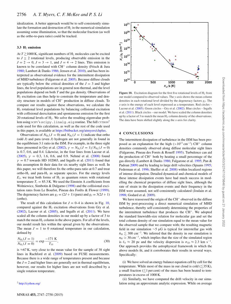
Finally, to gauge the spatial extent of these regions, we show inFig. 9 the result of integrating NCH+ and NH along each of the eightrays in Table 2. All of the rays show the same general behaviour:there are large regions that make basically no contribution to CH+

Figure 8. Blue – average histogram of CH+ column densities over 2500lines of sight passing through the simulation volume. The error bars indicatethe 1σ range of variation over all 50 samples of 50 sight lines each. Red– histogram of the CH+ column densities from the 50 sight line sample inWeselak et al. (2008).

column, punctuated by a few thin zones where the CH+ abundanceis substantial. The typical sight line intersects approximately twoto four of these regions. This analysis further confirms the viewof Falgarone & Puget (1995) – that the cold ISM contains isolatedpatches of hot, chemically active gas, and that these regions arecrucial to understanding diffuse cloud chemistry.

The gas densities we infer for the CH+-containing regions in ourmodel are lower than those typically associated with gas containingsubstantial abundances of H2. As discussed in Section 2.5, a sub-stantial H2 fraction is crucial for CH+ formation, and our modelsuggests that low densities are crucial, as well. However, it is notonly the local gas density that is important for setting the H2 frac-tion; the total shielding from the ambient radiation field matters aswell. In PDR models that assume constant density, this distinctionis not made, but in a supersonically turbulent medium, it is entirelypossible for a region with a low local gas density to nonetheless bewell shielded from FUV radiation. Indeed, Table 2 and Fig. 9 showthat, in our model, the CH+-forming regions tend to be randomlydistributed along sight lines, so that many of them would be wellshielded enough (AV greater than a few tenths) for molecules toform. That said, our adoption of a constant H2 fraction is clearly an

Figure 9. CH+ column density versus total column density NH integratedalong the same eight sight lines shown in Table 2. The quantities NCH+ (d)and NH(d) are the CH+ and total column densities integrated up though pathlength d along each ray. The x-axis has been normalized by the total columndensity NH(�0) to fit all the rays on the same plot.

MNRAS 453, 2747–2758 (2015)

Dow


ic.oup.com/m



idealization. A better approach would be to self-consistently simu-late the formation and destruction of H2 in the numerical simulationassuming some illumination, so that the molecular fraction (as wellas the ortho-to-para ratio) could be tracked.

3.3 H2 emission

At T �1000 K, significant numbers of H2 molecules can be excitedto J ≥ 2 rotational levels, producing observable emission in theJ = 2 → 0, J = 3 → 1, and J = 4 → 2 lines. This emission isknown to be correlated with CH+ column density (Frisch & Jura1980; Lambert & Danks 1986; Jensen et al. 2010), and has been in-terpreted as observational evidence for the intermittent dissipationof MHD turbulence (Falgarone et al. 2005). Because diffuse cloudsare typically below the critical densities of the J = 3 and higherlines, the level populations are in general non-thermal, and the levelpopulations depend on both T and the gas density. Observations ofH2 excitation can thus help to constrain the temperature and den-sity structure in models of CH+ production in diffuse clouds. Tocompare our results against these observations, we calculate theH2 rotational level populations by balancing collisional excitationwith collisional deexcitation and spontaneous emission for the first20 rotational levels of H2. We solve the resulting eigenvalue prob-lem using SCIPY’s scipy.linalg.eig routine. The full CYTHON2

code used for this calculation, as well as the rest of the code usedin this paper, is available at https://bitbucket.org/atmyers/chplus.

Observations of NH2 (J = 0) and NH2 (J = 1) indicate that ortho(odd J) and para (even J) hydrogen are not generally in found inthe equilibrium 3:1 ratio in the ISM. For example, in the three sightlines presented in Gry et al. (2002), γ = NH2 (J = 1)/NH2 (J = 0)is 0.7, 0.6, and 0.4. Likewise, in the four lines from Lacour et al.(2005), γ = 0.3, 1.6, 0.6, and 0.9. Nehme et al. (2008) foundγ = 0.7 towards HD 102065, and Ingalls et al. (2011) found thatthis assumption fit their data for six nearby sight lines as well. Inthis paper, we will therefore fix the ortho:para ratio at 0.7 and treatortho-H2 and para-H2 as separate species. For the energy levelsEJ, we treat both forms of H2 as quantum rotors with rotationaltemperature Tr = 85.3 K. We used the Einstein A coefficients fromWolniewicz, Simbotin & Dalgarno (1998) and the collisional exci-tation rates from Le Bourlot, Pineau des Forets & Flower (1999).The degeneracy factors are gJ = (2J + 1) (para) and gJ = 3(2J + 1)(ortho).

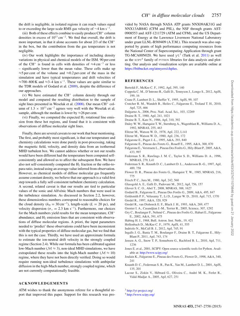
The result of this calculation for J = 0–4 is shown in Fig. 10,compared against the H2 excitation observations from Gry et al.(2002), Lacour et al. (2005), and Ingalls et al. (2011). We havescaled all the column densities in our model up by a factor of 3 tomatch the mean H2 column in the above papers. For all of the levels,our model result lies within the spread given by the observations.The mean J = 1 to 0 rotational temperature in our calculation,defined by

NH2 (J = 1)

NH2 (J = 0)= exp

−171 K

T10, (30)

is ≈67 K, very close to the mean value for the sample of 38 sightlines in Rachford et al. (2009) based on FUSE measurements.Because there is a wide range of temperatures present and becausethe J = 2 and higher lines are generally not in thermal equilibrium,however, our results for higher lines are not well described by asingle rotation temperature.

2 http://cython.org/

Figure 10. Excitation diagram for the first five rotational levels of H2 fromour model compared to observed values. The y-axis shows the mean columndensities in each rotational level divided by the degeneracy factors gJ. Thex-axis is the energy of each level expressed as a temperature. Red circles –Lacour et al. (2005). Green circles – Gry et al. (2002). Blue circles – Ingallset al. (2011). Black circles – our model. We have scaled the column densitiesup by a factor of 3 to match the mean H2 column density of the observations.The data have been shifted slightly along the x-axis for clarity.

4 C O N C L U S I O N S

The intermittent dissipation of turbulence in the ISM has been pro-posed as an explanation for the high (>1013 cm−2) CH+ columndensities commonly observed along diffuse molecular sight lines(Falgarone, Pineau des Forets & Roueff 1995). Turbulence can aidthe production of CH+ both by heating a small percentage of thegas directly (Lambert & Danks 1986; Falgarone et al. 1995; Pan &Padoan 2009) and by leading to large drift velocities (Spaans 1995;Federman et al. 1996; Sheffer et al. 2008) within localized regionsof intense dissipation. Detailed dynamical and chemical models ofthese intense dissipation events have had much success in mod-elling the chemical properties of diffuse sight lines, although therate of strain in the dissipation events and their frequency in theISM were assumed, not self-consistently calculated (Joulain et al.1998; Godard et al. 2009).

We have reassessed the origin of the CH+ observed in the diffuseISM by post-processing a direct numerical simulation of MHDturbulence, thereby self-consistently determining the properties ofthe intermittent turbulence that produces the CH+. We adoptedthe standard linewidth-size relation for molecular gas and set thetotal column density of our simulation equal to the mean value forthe observed sample that we compare with; the resulting magneticfield in our simulation ∼5 μG is typical for interstellar gas withnH � 300 cm−3. We inferred that the density in our simulation isnH 30 cm−3, which implies that the size of the simulated regionis �0 ≈ 20 pc and the velocity dispersion is σ1D ≈ 2.3 km s−1.Our approach provides the astrophysical framework in which theabove models fit, and it corroborates their results in several ways.Specifically:

(i) We have solved an energy balance equation cell by cell for thetemperature. While most of the mass in our cloud is cold (�35 K),a small fraction (�1 per cent) of the mass has been heated to tem-peratures in excess of 1000 K.

(ii) Similarly, we have computed the drift velocity in our simu-lation using an approximate analytic expression. While on average

MNRAS 453, 2747–2758 (2015)

Dow


ic.oup.com/m


https://bitbucket.org/atmyers/chplus

http://cython.org/


the drift is negligible, in isolated regions it can reach values equalto or exceeding the large-scale RMS gas velocity of ∼4 km s−1.

(iii) Both of these effects combine to easily produce CH+ columndensities in excess of 1013 cm−2. We find that overall, the drift ismore important, in that it alone accounts for about 2/3 of the CH+

in the box, but the contribution from the gas temperature is notnegligible.

(iv) Our work highlights the importance of including densityvariations in physical and chemical models of the ISM. 90 per centof the CH+ is found in cells with densities of ≈4 cm−3 or less– significantly lower than the mean value. These cells make up≈5 per cent of the volume and ≈0.2 per cent of the mass in thesimulation and have typical temperatures and drift velocities of≈700–800 K and ≈3–4 km s−1. These values are quite similar tothe TDR models of Godard et al. (2009), despite the difference ofour approaches.

(v) We have estimated the CH+ column density through ourmodel and compared the resulting distribution to the sample ofsight lines presented in Weselak et al. (2008). Our mean CH+ col-umn of 1.3 × 1013 cm−2 agrees very well with the Weselak et al.sample, although the median is lower by ≈26 per cent.

(vi) Finally, we computed the expected H2 rotational line emis-sion from these hot regions, and found that it is consistent withobservations of diffuse molecular sight lines.

Finally, there are several caveats to our work that bear mentioning.The first, and probably most significant, is that our temperature andchemistry calculations were done purely in post-processing, takingthe magnetic field, velocity, and density data from an isothermalMHD turbulent box. We cannot address whether or not our resultswould have been different had the temperature been computed self-consistently and allowed us to affect the subsequent flow. We havealso not self-consistently computed the H2 fraction or the ortho-to-para ratio, instead using an average value inferred from observation.However, as chemical models of diffuse molecular gas frequentlyassume constant density, we believe that our approach is a valid firststep towards a fully self-consistent turbulent chemistry calculation.A second, related caveat is that our results are tied to particularvalues of the sonic and Alfvenic Mach numbers that were used inthe turbulence simulation. As discussed in Section 2.2, however,these dimensionless numbers correspond to reasonable choices forthe cloud density (nH = 30 cm−3), length-scale (L = 20 pc), andvelocity dispersion (σ v = 2.3 km s−1). Furthermore, our choicesfor the Mach numbers yield results for the mean temperature, CH+

abundance, and H2 emission lines that are consistent with observa-tions of diffuse molecular regions. A priori, the input parametersneeded to ‘predict’ these observations could have been inconsistentwith the typical properties of diffuse molecular gas, but we find thatthis is not the case. Thirdly, we have used an approximate formulato estimate the ion-neutral drift velocity in the strongly coupledregime (Section 2.4). While our formula has been calibrated againstlow-Mach number (M ≈ 3), non-ideal MHD simulations, we haveextrapolated these results into the high-Mach number (M ≈ 10)regime, where they have not been directly verified. Doing so wouldrequire running non-ideal turbulence simulations with ambipolardiffusion in the high-Mach number, strongly coupled regime, whichare not currently computationally feasible.

AC K N OW L E D G E M E N T S

ATM wishes to thank the anonymous referee for a thoughtful re-port that improved this paper. Support for this research was pro-

vided by NASA through NASA ATP grants NNX09AK31G andNNX13AB84G (CFM and PSL), the NSF through grants AST-0908553 and AST-1211729 (ATM and CFM), and the US Depart-ment of Energy at the Lawrence Livermore National Laboratoryunder grant LLNL-B569409 (A.T.M.). This research was also sup-ported by grants of high performance computing resources fromthe National Center of Supercomputing Application through grantTG-MCA00N020. We have used yt3 (Turk et al. 2011) as wellas the SCIPY4 family of PYTHON libraries for data analysis and plot-ting. Our analysis and visualization scripts are available online athttps://bitbucket.org/atmyers/chplus.

R E F E R E N C E S

Bertoldi F., McKee C. F., 1992, ApJ, 395, 140Coppola C. M., D’Introno R., Galli D., Tennyson J., Longo S., 2012, ApJS,

199, 16Crane P., Lambert D. L., Sheffer Y., 1995, ApJS, 99, 107Crutcher R. M., Wandelt B., Heiles C., Falgarone E., Troland T. H., 2010,

ApJ, 725, 466Dalgarno A., 2006, Proc. Natl. Acad. Sci., 103, 12269Draine B. T., 1980, ApJ, 241, 1021Draine B. T., Katz N., 1986, ApJ, 310, 392Duley W. W., Hartquist T. W., Sternberg A., Wagenblast R., Williams D. A.,

1992, MNRAS, 255, 463Elitzur M., Watson W. D., 1978, ApJ, 222, L141Elitzur M., Watson W. D., 1980, ApJ, 236, 172Falgarone E., Puget J.-L., 1995, A&A, 293, 840Falgarone E., Pineau des Forets G., Roueff E., 1995, A&A, 300, 870Falgarone E., Verstraete L., Pineau Des Forets G., Hily-Blant P., 2005, A&A,

433, 997Federman S. R., Rawlings J. M. C., Taylor S. D., Williams D. A., 1996,

MNRAS, 279, L41Federman S. R., Knauth D. C., Lambert D. L., Andersson B.-G., 1997, ApJ,

489, 758Flower D. R., Pineau des Forets G., Hartquist T. W., 1985, MNRAS, 216,

775Frisch P. C., Jura M., 1980, ApJ, 242, 560Glassgold A. E., Galli D., Padovani M., 2012, ApJ, 756, 157Glover S. C. O., Abel T., 2008, MNRAS, 388, 1627Godard B., Falgarone E., Pineau Des Forets G., 2009, A&A, 495, 847Goldsmith P. F., Velusamy T., Li D., Langer W. D., 2010, ApJ, 715, 1370Gredel R., 1997, A&A, 320, 929Gredel R., van Dishoeck E. F., Black J. H., 1993, A&A, 269, 477Grenier I. A., Casandjian J.-M., Terrier R., 2005, Science, 307, 1292Gry C., Boulanger F., Nehme C., Pineau des Forets G., Habart E., Falgarone

E., 2002, A&A, 391, 675Habing H. J., 1968, Bull. Astron. Inst. Neth., 19, 421Hollenbach D., McKee C. F., 1979, ApJS, 41, 555Indriolo N., McCall B. J., 2012, ApJ, 745, 91Ingalls J. G., Bania T. M., Boulanger F., Draine B. T., Falgarone E., Hily-

Blant P., 2011, ApJ, 743, 174Jensen A. G., Snow T. P., Sonneborn G., Rachford B. L., 2010, ApJ, 711,

1236Jones E. et al., 2001, SCIPY: Open source scientific tools for Python. Avail-

able at: http://www.scipy.org/Joulain K., Falgarone E., Pineau des Forets G., Flower D., 1998, A&A, 340,

241Knauth D. C., Federman S. R., Pan K., Yan M., Lambert D. L., 2001, ApJS,

135, 201Lacour S., Ziskin V., Hebrard G., Oliveira C., Andre M. K., Ferlet R.,

Vidal-Madjar A., 2005, ApJ, 627, 251

3 http://yt-project.org/4 http://www.scipy.org/

MNRAS 453, 2747–2758 (2015)

Dow


ic.oup.com/m


https://bitbucket.org/atmyers/chplus

http://www.scipy.org/

http://yt-project.org/

http://www.scipy.org/


Lambert D. L., Danks A. C., 1986, ApJ, 303, 401Landau L. D., Lifshitz E. M., 1959, Fluid Mechanics. Pergamon Press,

OxfordLe Bourlot J., Pineau des Forets G., Flower D. R., 1999, MNRAS, 305, 802Li P. S., McKee C. F., Klein R. I., Fisher R. T., 2008, ApJ, 684, 380Li P. S., Martin D. F., Klein R. I., McKee C. F., 2012a, ApJ, 745, 139Li P. S., Myers A., McKee C. F., 2012b, ApJ, 760, 33Mac Low M.-M., 1999, ApJ, 524, 169McKee C. F., Ostriker E. C., 2007, ARA&A, 45, 565McKee C. F., Li P. S., Klein R. I., 2010, ApJ, 720, 1612Mathis J. S., Mezger P. G., Panagia N., 1983, A&A, 128, 212Nehme C., Le Bourlot J., Boulanger F., Pineau Des Forets G., Gry C., 2008,

A&A, 483, 485Pan L., Padoan P., 2009, ApJ, 692, 594Pan K., Federman S. R., Cunha K., Smith V. V., Welty D. E., 2004, ApJS,

151, 313Rachford B. L. et al., 2009, ApJS, 180, 125Ritchey A. M., Martinez M., Pan K., Federman S. R., Lambert D. L., 2006,

ApJ, 649, 788Shaw G., Ferland G. J., Srianand R., Abel N. P., van Hoof P. A. M., Stancil

P. C., 2008, ApJ, 675, 405Sheffer Y., Rogers M., Federman S. R., Abel N. P., Gredel R., Lambert

D. L., Shaw G., 2008, ApJ, 687, 1075Shu F. H., 1992, Physics of Astrophysics, Vol. II. University Science Books,

Mill Valley, CA

Snow T. P., McCall B. J., 2006, ARA&A, 44, 367Sofia U. J., Lauroesch J. T., Meyer D. M., Cartledge S. I. B., 2004, ApJ,

605, 272Sofia U. J., Parvathi V. S., Babu B. R. S., Murthy J., 2011, AJ, 141, 22Sonnentrucker P., Friedman S. D., Welty D. E., York D. G., Snow T. P.,

2002, ApJ, 576, 241Sonnentrucker P., Friedman S. D., Welty D. E., York D. G., Snow T. P.,

2003, ApJ, 596, 350Spaans M., 1995, PhD thesis, PhD thesis. Univ. Leiden, the NetherlandsSternberg A., Dalgarno A., 1995, ApJS, 99, 565Stone J. M., Ostriker E. C., Gammie C. F., 1998, ApJ, 508, L99Turk M. J., Smith B. D., Oishi J. S., Skory S., Skillman S. W., Abel T.,

Norman M. L., 2011, ApJS, 192, 9van Dishoeck E. F., Black J. H., 1986, ApJS, 62, 109Weselak T., Galazutdinov G., Musaev F., Krełowski J., 2008, A&A, 479,

149Wolfire M. G., McKee C. F., Hollenbach D., Tielens A. G. G. M., 2003,

ApJ, 587, 278Wolfire M. G., Hollenbach D., McKee C. F., 2010, ApJ, 716, 1191Wolniewicz L., Simbotin I., Dalgarno A., 1998, ApJS, 115, 293Zweibel E. G., Brandenburg A., 1997, ApJ, 478, 563

This paper has been typeset from a TEX/LATEX file prepared by the author.

MNRAS 453, 2747–2758 (2015)

Dow


ic.oup.com/m


The CH abundance in turbulent, diffuse molecular clouds

Documents