The Causes and Quantification of Population Vulnerability.

The Causes and Quantification of Population Vulnerability

Ecological and Genetic factors that threaten a population

(and may possible be mitigated through proper management)

• The life history of the species

• The average environment conditions

• The extrinsic variability in the biotic and abiotic factors influencing a population

• The intrinsic variability caused by small population sizes

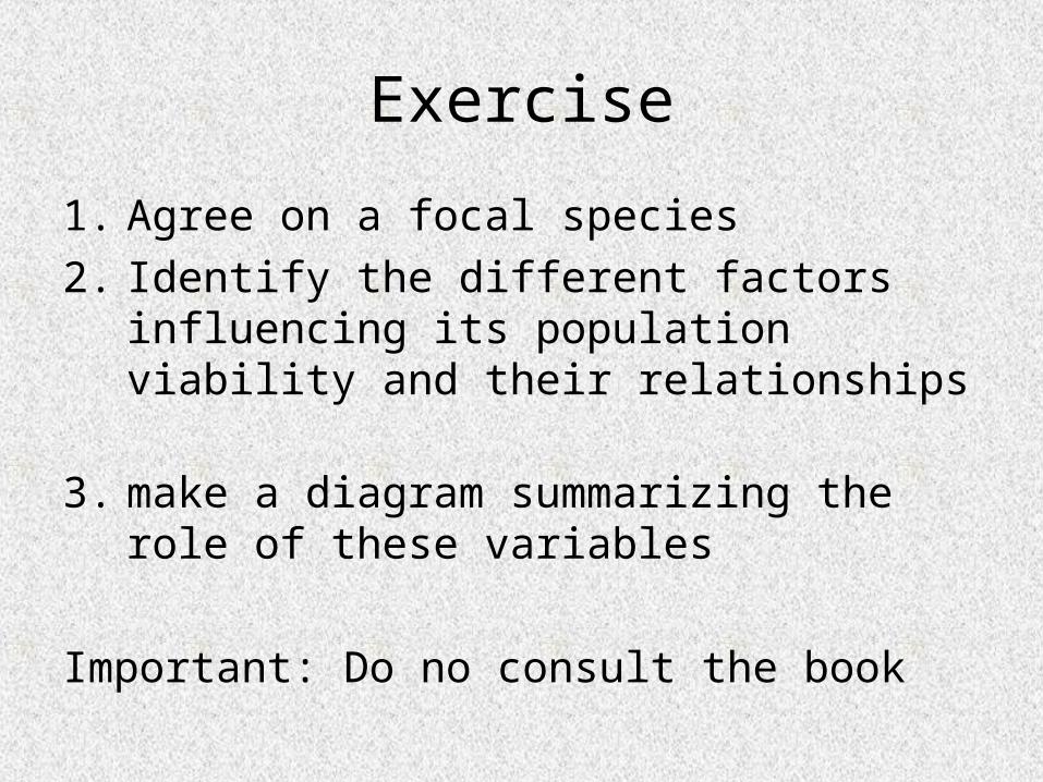
Exercise

1. Agree on a focal species

2. Identify the different factors influencing its population viability and their relationships

3. make a diagram summarizing the role of these variables

Important: Do no consult the book

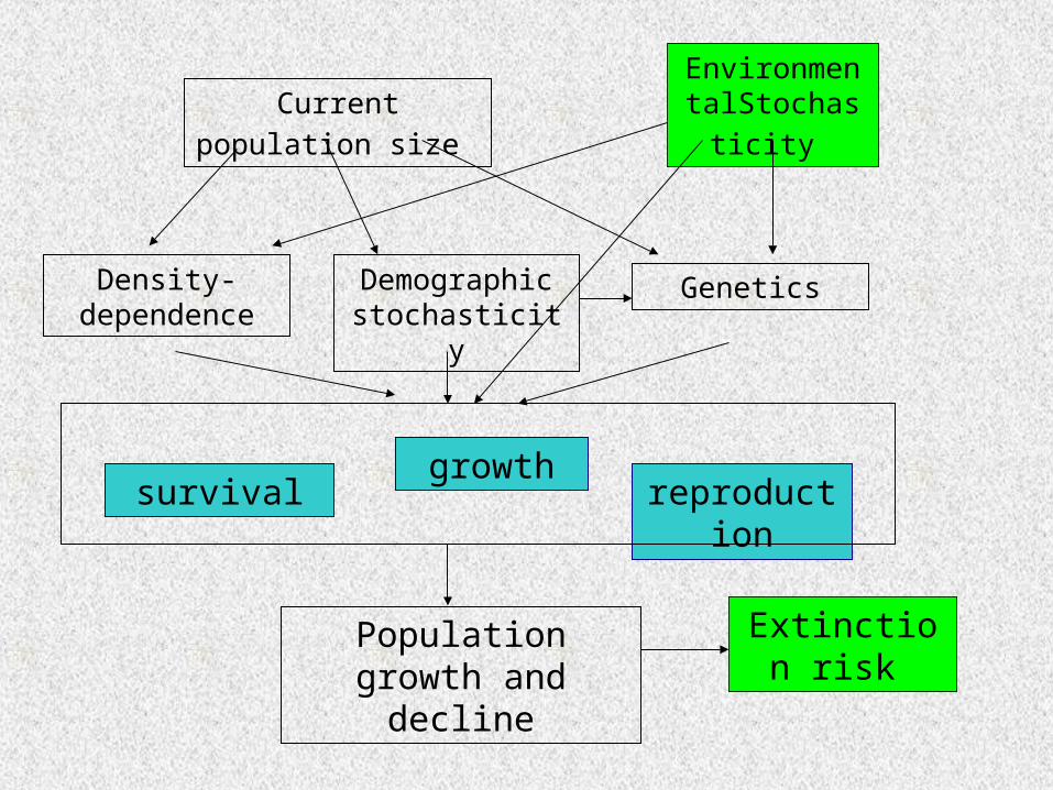
Current population size

Density-dependence

Demographic stochasticity

Genetics

survivalgrowth

reproduction

Population growth and decline

Environmental

Stochasticity

Extinction risk

Vital rates• Components of

individual performance:

Birth rate

Death rate

Growth rate

www.owlsonline.org/babyanimals.html

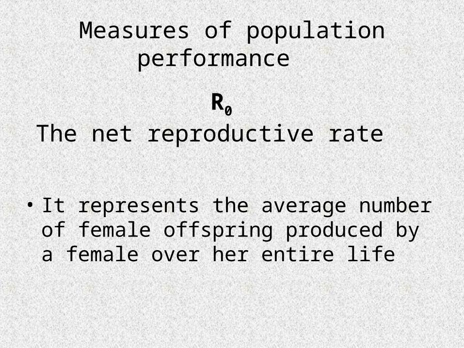
R0 The net reproductive rate

• It represents the average number of female offspring produced by a female over her entire life

Measures of population performance

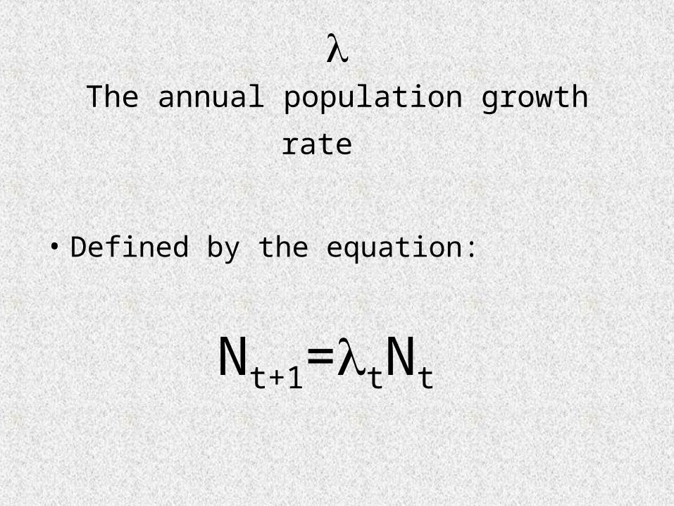
The annual population growth rate

• Defined by the equation:

Nt+1=tNt

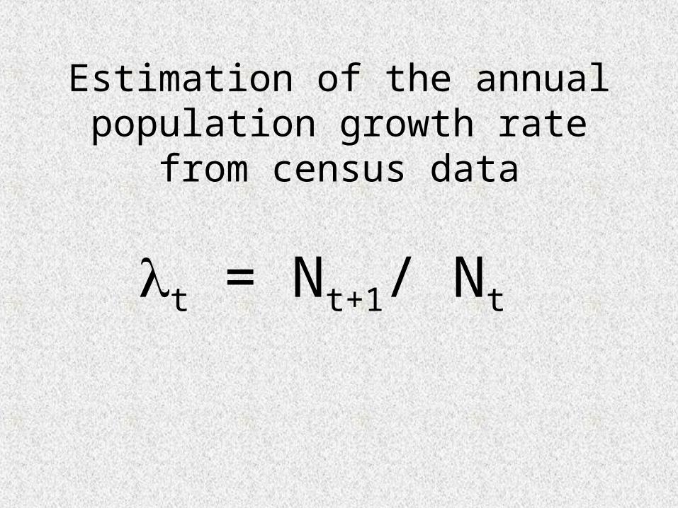
Estimation of the annual population growth rate from

census data

t = Nt+1/ Nt

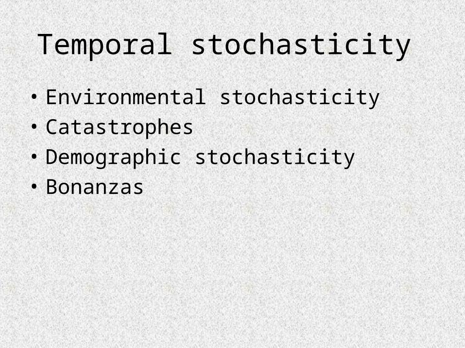
Temporal stochasticity

• Environmental stochasticity

• Catastrophes

• Demographic stochasticity

• Bonanzas

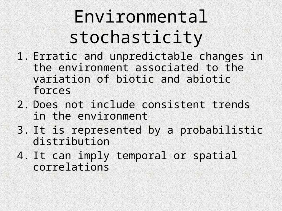
Environmental stochasticity

1. Erratic and unpredictable changes in the environment associated to the variation of biotic and abiotic forces

2. Does not include consistent trends in the environment

3. It is represented by a probabilistic distribution 4. It can imply temporal or spatial correlations

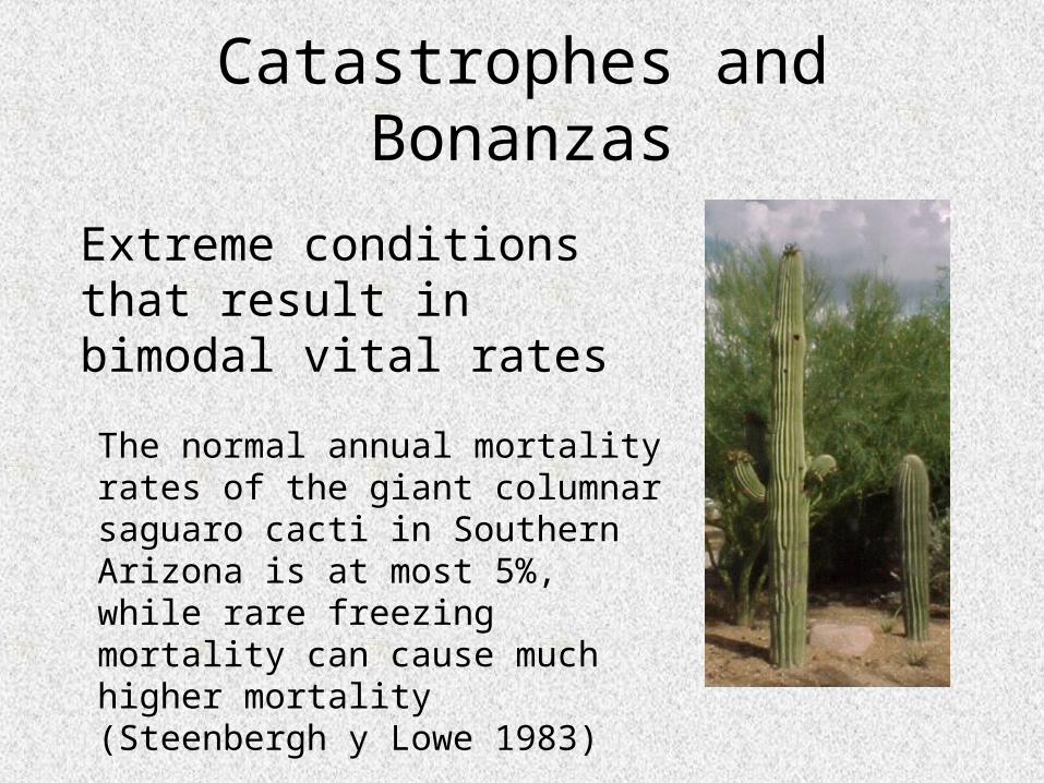
Catastrophes and Bonanzas

Extreme conditions that result in bimodal vital rates

The normal annual mortality rates of the giant columnar saguaro cacti in Southern Arizona is at most 5%, while rare freezing mortality can cause much higher mortality (Steenbergh y Lowe 1983)

Demographic stochasticity

• Temporal variation in population growth driven by chance variation in the actual fate of different individuals within a year

• Its magnitude strongly depends on population size

The California condorIn the last years there have been over 89 releases of condors raised in captivity. The individual annual survival rate of 28 birds released in Arizona was estimated 0.85 (Meretsky et al. 2000).

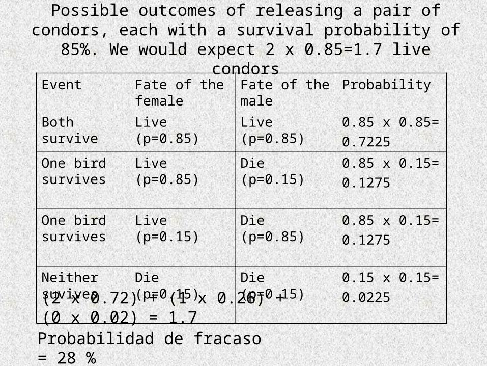
Possible outcomes of releasing a pair of condors, each with a survival probability of 85%. We would expect 2 x 0.85=1.7

live condors

Event Fate of the female

Fate of the male

Probability

Both survive Live (p=0.85) Live (p=0.85) 0.85 x 0.85=

0.7225

One bird survives

Live (p=0.85) Die (p=0.15) 0.85 x 0.15=

0.1275

One bird survives

Live (p=0.15) Die (p=0.85) 0.85 x 0.15=

0.1275

Neither suvives

Die (p=0.15) Die (p=0.15) 0.15 x 0.15=

0.0225

(2 x 0.72) + (1 x 0.26) + (0 x 0.02) = 1.7

Probabilidad de fracaso = 28 %

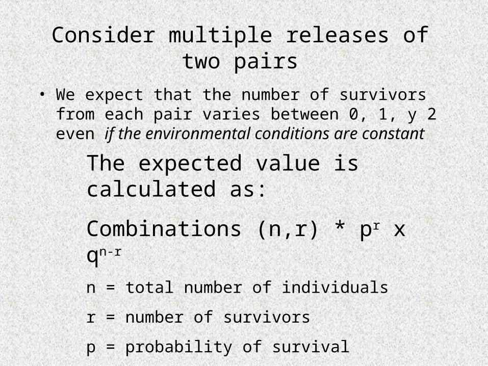
Consider multiple releases of two pairs

• We expect that the number of survivors from each pair varies between 0, 1, y 2 even if the environmental conditions are constant

The expected value is calculated as:

Combinations (n,r) * pr x qn-r

n = total number of individuals

r = number of survivors

p = probability of survival

q = probability of dying

2 4 8 16 32 64 1280 2 0 0 0 0 0 0

0-0.1 0 0 0 0 0 0 00.1-0.2 0 0 0 0 0 0 00.2-0.3 0 1 0 0 0 0 00.3-0.4 0 0 0 0 0 0 00.4-0.5 26 10 0 0 0 0 00.5-0.6 0 0 2 2 0 0 00.6-0.7 0 0 8 6 2 0 00.7-0.8 0 37 24 13 18 15 60.8-0.9 0 0 38 51 53 71 89

0.9-1 0 0 0 21 27 14 41 72 52 27 7 1 0 0

Percentage of populations expected to show different observed survival rates under demographic stochasticity

RatePopulation size

• Demographic stochasticity can impact the future of populations.

• However is only significant in small populations.

• Bruce Kendall y Gordon Fox (2002) argue that it may less important than is usually predicted, due to the inherent differences in survival rates among individuals.

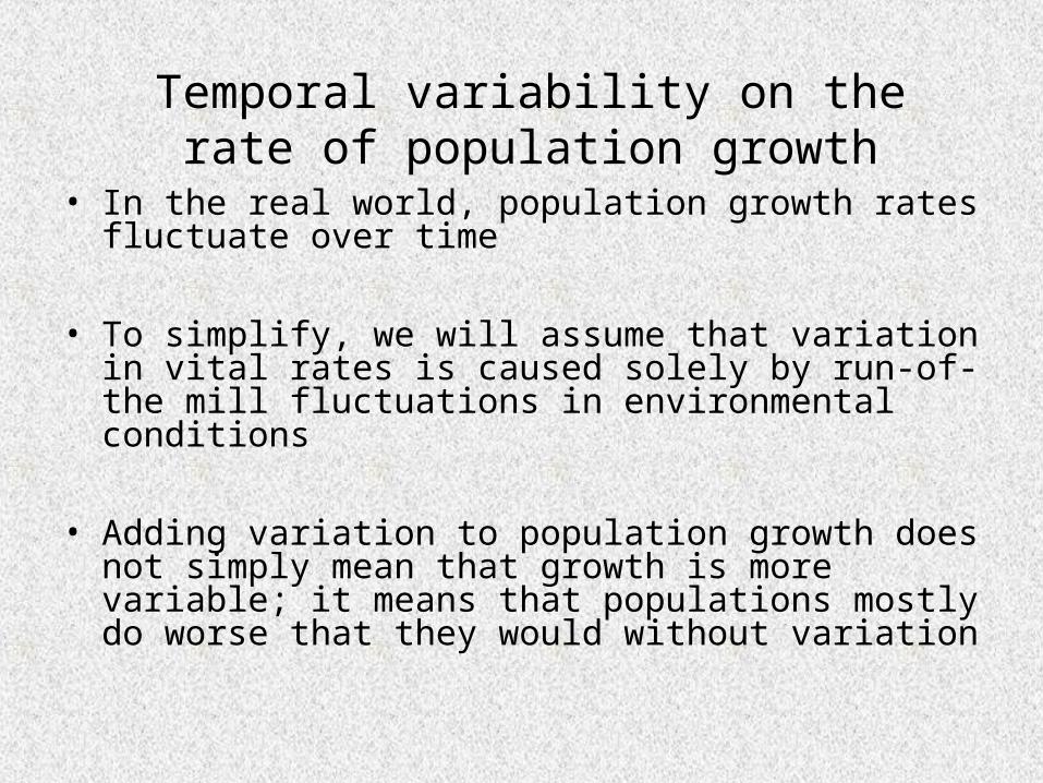
Temporal variability on the rate of population growth

• In the real world, population growth rates fluctuate over time

• To simplify, we will assume that variation in vital rates is caused solely by run-of-the mill fluctuations in environmental conditions

• Adding variation to population growth does not simply mean that growth is more variable; it means that populations mostly do worse that they would without variation

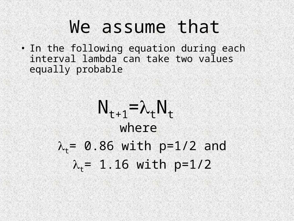
We assume that• In the following equation during each interval

lambda can take two values equally probable

Nt+1=tNt where

t= 0.86 with p=1/2 and

t= 1.16 with p=1/2

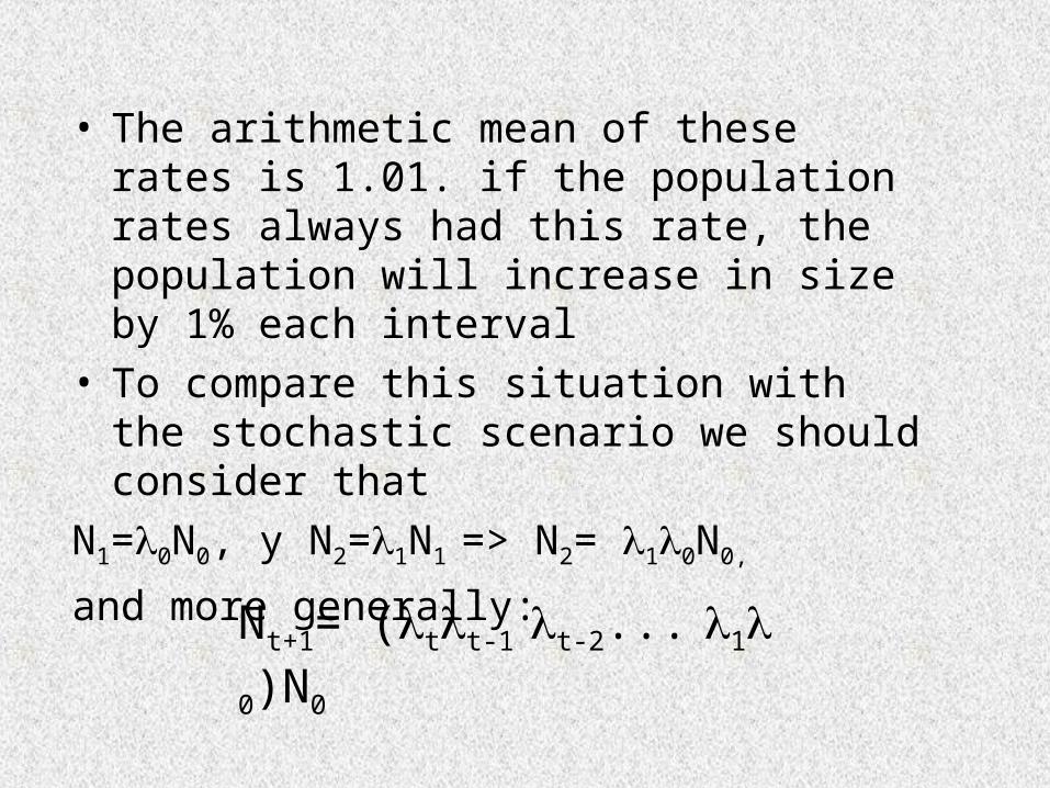
• The arithmetic mean of these rates is 1.01. if the population rates always had this rate, the population will increase in size by 1% each interval

• To compare this situation with the stochastic scenario we should consider that

N1=0N0, y N2=1N1 => N2= 10N0,

and more generally:

Nt+1= (tt-1 t-2... 1 0)N0

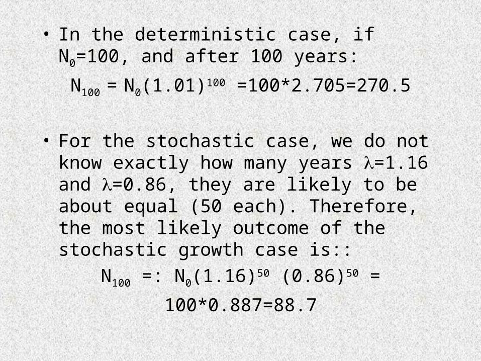
• In the deterministic case, if N0=100, and after 100 years:

N100 = N0(1.01)100 =100*2.705=270.5

• For the stochastic case, we do not know exactly how many years =1.16 and =0.86, they are likely to be about equal (50 each). Therefore, the most likely outcome of the stochastic growth case is::

N100 =: N0(1.16)50 (0.86)50 =

100*0.887=88.7

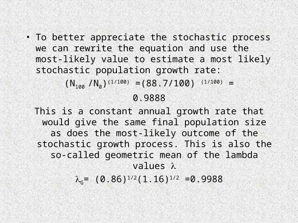
• To better appreciate the stochastic process we can rewrite the equation and use the most-likely value to estimate a most likely stochastic population growth rate:

(N100 /N0)(1/100) =(88.7/100) (1/100) =

0.9888

This is a constant annual growth rate that would give the same final population size as does the most-likely

outcome of the stochastic growth process. This is also the so-called geometric mean of the lambda

values G= (0.86)1/2(1.16)1/2 =0.9988

Spatial variability

• The means and variances of the vital rates, and hence of population growth rates, will usually not be equal across all sites and habitats.

• The most serious complication in a multi-site situation arises due to correlations in the temporal variation across sites.

• Movement of individuals between populations

Observation Error

• Both vital rates and population counts will usually reflect the influence of population error

• It merely reflect our inability to measure vital rates or population growth size with absolute precision, and so has no effect on viability

• Nevertheless, introduce biases and uncertainty into our estimates of population viability

The importance of the sampling design

Some examples:

• Do sampling in what we think is the best habitat.

• There is a bias to the most robust plants or less fit animals.

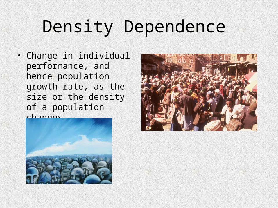
Density Dependence

• Change in individual performance, and hence population growth rate, as the size or the density of a population changes

Negative density dependence • It is a decline in average vital rates as

population size increases

• It is typically caused by intraspecific competition for limited resources or by interacting species whose impacts increase proportionally as the density of the focal organism increases

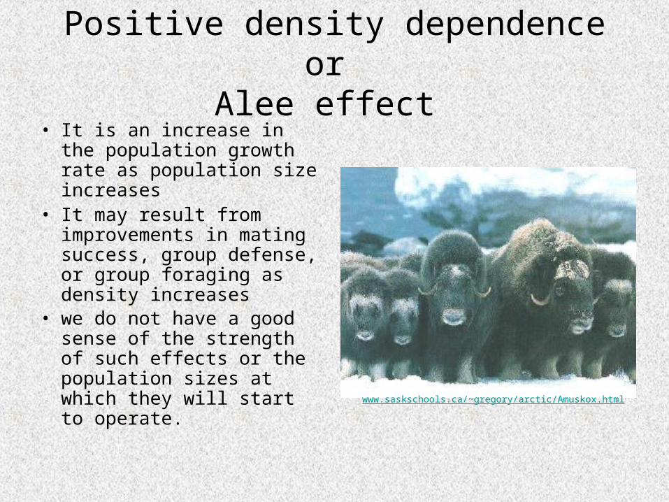
Positive density dependence or Alee effect

• It is an increase in the population growth rate as population size increases

• It may result from improvements in mating success, group defense, or group foraging as density increases

• we do not have a good sense of the strength of such effects or the population sizes at which they will start to operate.

www.saskschools.ca/~gregory/arctic/Amuskox.html

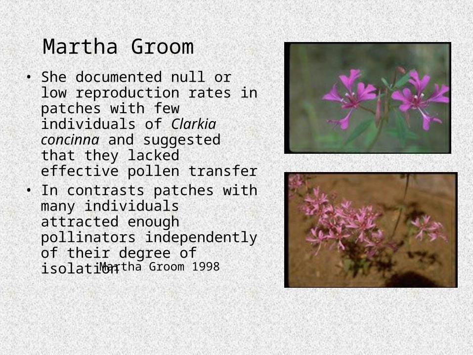
Martha Groom• She documented null or low

reproduction rates in patches with few individuals of Clarkia concinna and suggested that they lacked effective pollen transfer

• In contrasts patches with many individuals attracted enough pollinators independently of their degree of isolation

Martha Groom 1998

Some considerations about density dependence

• Generally we lack information on its manifestation

• Due to the sensibility of the models to these factors and the data limitations, it is reasonable to define:1. higher thresholds beyond which the population does not growth 2. Quasi-extinction thresholds high enough to avoid that Alee effects are significant

Genetic factors Concepts

• Heterozygosity: It is an indicator of genetic diversity: the probability that, for the average locus, there will be two different alleles

• Inbreeding: the average probability that an individual’s two copies of a gene are “identical by descent”

• Inbreeding depression is commonly estimated as a certain percentage reduction in some vital rate with a given increase in inbreeding level

Genetic FactorsIndicators

Quantifying Population Viability

• Viable populations are those that have a suitable low chance of going extinct before a specified future time.

• Quasi-extinction thresholds

• (Ginzburg et al. 1982)http://life.bio.sunysb.edu/ee/people/ginzbgindex.html

Lev Ginzburg

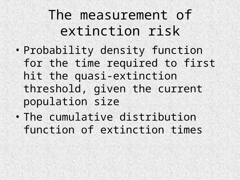
The measurement of extinction risk

• Probability density function for the time required to first hit the quasi-extinction threshold, given the current population size

• The cumulative distribution function of extinction times

Viability metrics

• The probability of extinction by a given time

• The ultimate probability of extinction

• Mean, median and mode of the predicted extinction times (given that it occurs eventually)

Which one?

0.0000

0.0002

0.0004

0.0006

0.0008

0.0010

0.0012

0.0014

0.0016

0.0018

0.0020

0 10 20 30 40 50 60

Años en el futuro

Pro

ba

bil

ida

d a

cu

mu

lad

a d

e c

ua

si-

ex

tin

cio

n

Cumulative extinction probability of the Grizzly bears at Yellowstone. The x-axes indicates the time required for a population of 99 females to decrease to 20

Si la distribución probabilística de t se aproxima a la lognormal, la magnitud de la depresión en la

tasa estocástica se puede calcular como

0.6

0.8

1

1.2

0 0.2 0.4 0.6 0.8 1 1.2

Desviacion estandar de lambda

Ta

sa e

sto

cast

ica

de

cre

cim

ien

to

1.05

0.95

G= A/(1+2/ A

2)

Caughley dichotomy

• Small population paradigm: emphasizing the role of stochastic factors

• Decline population paradigm: focused on the deterministic factors that lead to positive or negative population growth rates

: www.science.org.au/academy/memoirs/caughley.htm