The Campaign Context for Partisanship Stability ·  · 2011-03-31The Campaign Context for Partisanship Stability* J. Quin Monson ... Campaign Analysis Project ... general observation

The Campaign Context for Partisanship Stability*

J. Quin Monson

Kelly D. Patterson

Jeremy C. Pope

Brigham Young University

Center for the Study of Elections and Democracy

Abstract

Much previous research shows that partisanship is among the most stable concepts in political behavior. Despite this consensus there is evidence of partisan change. We ask an intermediate question: under what conditions is partisanship more or less stable? We use 2008 Cooperative Campaign Analysis Project (CCAP) data to examine the stability of partisan identification within the context of the 2008 presidential election campaigns. The results of our models suggest that stability is clearly related to an individual’s location within the campaign environment. Respondents living in presidential “battleground” states and receiving the most intense campaign messages are very likely to remain stable, as are voters at the opposite end of the spectrum. Voters in between these extremes appear to be somewhat more susceptible to change, even within the context of a single election. We theorize that the stability of partisanship among certain segments of voters is the result of a competitive context that is able to activate a citizen’s underlying dispositions to support a party.

* Paper presented at the 2009 State of the Parties Conference, Akron, Ohio.

2

“Partisanship” is one of the most widely used concepts in political science, making

appearances in all of the sub-literatures that relate to elections. In spite of its importance to

voting behavior and elections, significant questions remain about the nature of partisanship and

the best ways to measure it. Some researchers argue that partisanship has a dynamic dimension

that means voters shift their allegiance in response to different political factors. Others argue

that partisanship is stable and that most variation in individual preferences results from some

form of measurement error. These two positions on the nature of partisanship bracket a more

basic question: under what conditions is partisanship more or less stable?

Citizen inattention to politics seems to suggest that the most frequent opportunity for

citizens to assess their partisanship come in the context of political campaigns. This is not to say

that other political events (e.g., debate over a war, a major piece of legislation, or a presidential

appointment) will not lead individuals to reflect on their partisanship. But the most

consistently presented chances to question partisan allegiances are the regularly scheduled

campaigns, making the key question for this paper: how does the campaign context affect

partisan stability?

1. The Nature of Partisanship

Though it is not our intention to resolve long-standing debates about the nature of

partisanship in this short article, a review of that literature is an important prelude to our

discussion of the campaign context for partisanship stability.

The publication of Voting (1954) by Berelson, Lazarsfeld, and McPhee and The American

Voter (1960) by Campbell et al. established partisanship as a psychological attachment to the

3

political parties. This attachment contained both cognitive and affective dimensions.

Individuals identified with a party because of its issue positions and also because of feelings

they may have about the parties. The authors of The American Voter and subsequent researchers

adopted the view that an individual’s party identification reflected long-term forces of

socialization. They also argued that partisanship was slow to change. If change occurred at all,

it was produced by significant changes in the life cycle (e.g. relocating to a new area) or major

political events (e.g. war, economic crisis). The authors of The American Voter conclude that “A

general observation about the political behavior of Americans is that their partisan preferences

show great stability between elections.” (Campbell et al. 1960, 120). Scholars argued for the

existence of microlevel stability even while demonstrating that macropartisanship changed in

response to assessments of the president and the confidence expressed by consumers (Erikson,

Mackuen, and Stimson 1989; Erikson, Mackuen, and Stimson 1998).

Other researchers focused on the possibility that partisanship may be more dynamic

than The American Voter (AV) and some of the subsequent models specified. Various research

traditions developed almost simultaneously with the AV model that allowed for short-term

factors to influence the partisanship of an individual. For example, the early rational choice

model posited that party identification results from the issue preferences of individuals or is in

some respect the summation of their different issue preferences (Downs 1957). This theory

allows for partisanship to change because individuals, when confronted with new information

about the positions of parties, could revise their commitment to a party. Other short-term

factors were identified that may also cause an individual to change party preferences or at least

the strength of those preferences. These short-term factors included assessment of the political

4

parties and their performance on issues (Page and Jones 1979; Fiorina 1981; Franklin and

Jackson 1983; Franklin 1992) and candidate personalities (Brody and Rothenberg 1988).

Electoral systems can also affect the commitment of individuals to their party (Finkel and

Scarrow 1985; Bowler, Lanoue, and Savoie 1994). All of this research assumes that partisanship

can change in response to changes in individual preferences or changes in the institutional

environment.

A more recent entry into the theoretical debate comes from social identity theory. This

theory holds that the groups to which one belongs—or at least they believe to which they

belong—comprise an important element of their social self and help them to define who they

are (Hogg, Terry, and White 1995; Stets and Burke 2000). It also helps to explain how

individuals develop and keep partisan attitudes and behaviors (Green, Palmquist, and Schickler

2002; Greene 2004). However, it does not necessarily solve the debate over the dynamics of

partisanship because the theory, with certain extensions, allows for individuals to reassess their

party identification depending on the kinds of cues and stimuli they receive from the political

environment (Greene 2004). At some level, social identity theory is compatible with the

rationalist accounts that emphasize short-term factors or the psychological accounts that

emphasize long-term socialization.

The debate over the dynamics of partisanship also depends heavily on the data and

methods selected by researchers to try to detect change. Researchers have mostly used panel

data to model the effects of change, but they have also used other types of survey data

including rolling aggregate data (Allsop and Weisberg, 1988), experimental data (Niemi, Reed,

and Weisberg, 1991), and cross-sectional data (Page and Jones, 1979). The debate over stability

5

has also been complicated by such factors as the time between the waves of the panels and how

exactly to conceptualize change across the separate waves. Finally, researchers have argued

that measurement error must also be included in any effort to model partisan change. Indeed,

they find that when measurement error is accounted for in the model that the effects of other

variables on partisan change become insignificant (Green and Palmquist, 1990; and Green,

Palmquist, and Schickler, 2002).

Typically this literature has focused on achieving better measures of partisanship,

without substantial attention to modeling consistency in partisan affiliations. Debates have

centered on the meaning of real change or whether or not instability is an artifact of

measurement error. But if voters are ambivalent about their partisan affiliation because of their

personal positions on issues or their knowledge of politics (think of a pro-life Democrat or

someone considering politics for the first time) their attachments may not be very stable.

Uncertainty, ambivalence and outright ignorance may create significant instability in

partisanship. We turn now to a description of that instability and a discussion of the

institutional context for that instability. The best place to begin is with the most regular of

political events: the scheduled campaign season.

2. Battlegrounds, Campaign Context, and Stability in Partisanship

Scholars of campaigns and elections have long been interested in the extent and source

of campaign effects. The accumulation of research in this area indicates that across a wide

spectrum of behavioral phenomena campaigns matter. Much of the research focuses on the

persuasive effects of campaigns, such as whether or not campaigns play an important role in

6

vote choice (e.g. Hillygus and Jackman 2003). Other research examines the effect of campaigns

on levels of political knowledge and interest (e.g. Gronke 2000).

More recently, scholars of campaign effects have sought to assess their impact by

studying voters who reside in battleground and non-battleground states during presidential

elections. Battleground states are those states where presidential candidates expend their time

and resources in an effort to secure the electoral votes cast by those states. Already, a rich

literature exists emphasizing the differences in campaign strategies and resources across states

that candidates believe are competitive (e.g. Shaw 1999, 2006). These strategic choices result in

the creation of different campaign contexts for citizens. States designated as “battlegrounds”

receive more attention from the candidates and the political parties (Shaw 2006, McClurg and

Holbrook 2009; Wolak 2006). The information-rich environments and the efforts made to

contact and mobilize voters help to stimulate turnout among previously inactive voters

(Gimpel, Kaufman, and Pearson-Merkowitz 2007), structure the vote choice for individuals

(McClurg and Holbrook 2009), and reduce uncertainty for voters (Jackman and Vavreck 2009a).

The idea of a battleground raises interesting questions for the issue of partisanship. If

we begin with an expectation that most voters possess and can express a “true” underlying

partisanship we would expect some voters in some campaign contexts to be better at giving

consistent answers than other voters. In other words, some voters apparently do not know how

to map their beliefs and ideas into the categories presented by the question. This inability may

be a consequence of their uncertainty about the parties or their ambivalence about how to label

themselves. If, as suggested by Zaller (1992) voters are answering questions with whatever

considerations come to mind at the moment the question is posed, they may be plagued by

7

ambivalence due to conflicts between their political beliefs and their partisanship or they may

be burdened by uncertainty about the positions of the parties1 and how their own beliefs should

map on to those positions. However, voters in an environment teeming with information about

the campaigns, the parties, and the issue positions, should have an easier time acquiring

information and using that information to help them more firmly grasp their partisanship.

It seems important to divide this campaign environment into two categories: residence

and campaign volume. In this formulation, residence in the battleground states should more

efficiently activate the latent preferences voters already have (Lazarsfeld, Berelson, and Gaudet

1944; Finkel 1993; Gelman and King 1993), thereby reducing voter uncertainty and ambivalence

and therefore reducing partisanship instability. The analysis below confirms much of our

intuition. Being in an intense campaign simply forces voters to consider their viewpoints and

reject alternative arguments. It seems likely that the presence of a hotly contested election

would significantly increase partisanship stability.

Residence Hypothesis: Living in a presidential “battleground” state should increase partisanship stability as the welter of messages, images, and arguments produces more considerations that lead to higher levels of certainty among voters.

But not all aspects of the “campaign” are created equal and simple residence in an

environment is far from the concept of saturation. Television advertisements are not the

equivalent of free media or mass mailings or telephone calls or face to face contact. Indeed

there is a campaigns literature that would suggest that these different media for the campaign

message should have different effects and be targeted at different levels to different individuals

1 Indeed it would make a lot of sense to be uncertain, given that political parties do often send conflicting messages.

8

and groups.2 Immersion in this campaign volume should also have a strong positive effect on

stability.

Campaign Volume Hypothesis: Immersion in the campaign messages should increase partisan stability as increased knowledge of the campaign messages produces higher levels of considerations to help a voter maintain partisan stability. Taken together the two hypotheses suggest that it is the combination of a strong

campaign context such as a battleground state along with contact with the campaigns that will

have the strongest effect. Citizens in a hotly contested context but are receiving relatively little

from the campaigns should be relatively less stable. In contrast the voters that live in the

battleground states and are receiving a high volume of campaign messages clearly have an

object to which they can pay close attention. They will not only discuss it more, read more

about it, hear more in the air, but also receive more campaign messages from television, in the

mail and via other means. The campaign messages are likely to have the strongest partisan

content and therefore are likely to have the strongest effects on partisan stability. Thus we

include an interaction hypothesis.

Interaction Hypothesis: Partisan stability should be strongest among those living in the battleground states and receiving the highest campaign volume.

These expectations are clearly enough to justify examining the data. So what exactly does it

say?

2 The literature is too voluminous to review in detail here. For a recent review of television advertising effects see Freedman, Franz, and Goldstein (2004). For a review of the effectiveness of other types of campaign communications see Green and Gerber (2004), Green and Gerber (2005), or Hillygus and Monson (2008).

9

3. Our Aims & Our Dataset

The 2008 election offered an opportunity to examine our hypotheses about partisan

stability in the context of a presidential election. We explore these ideas using data from the

2008 Cooperative Campaign Analysis Project (2008 CCAP) conducted by YouGov/Polimetrix.

CCAP is a large-scale panel survey conducted throughout the 2008 campaign.

The CCAP is a representative national sample similar to the slightly more well-known

Cooperative Congressional Election Survey (CCES).3 The CCAP sample was constructed using

an innovative model-assisted sampling technique. The process begins with a target sampling

frame from the 2005-2007 American Community Survey (ACS) using a variety of demographic

variables.4 With the target from the ACS defined, respondents were then chosen from the

YouGov/Polimetrix panel with an oversample in presidential battleground states and contacted

for the survey. For each wave of the panel all previous respondents were invited to participate

and fresh sample was added. The final pool of completed interviews totals approximately

48,000. The completed interviews from the YouGov/Polimetrix sample are then matched to the

ACS sampling frame using weighted Euclidean distances.5 Each individual in the ACS has

several possible matches among the completed interviews. Nearest neighbor matching is used

3 For more information about the 2008 CCAP see Jackman and Vavreck (2009b). 4 These include age, race, gender, education, marital status, number of children under 18, family income, employment status, citizenship, state, and metropolitan area. Voter registration and turnout from the November 2008 Current Population Survey Supplement was matched to this frame. Data on religious affiliation, church attendance, born again status, news interest, party identification, and ideology was matched from the 2007 Pew Religious Life Survey. For more details on the matching see Vavreck and Rivers (2008) and Jackman and Vavreck (2009c). 5 The distance function variables include the percentage survey waves completed, state, region, metropolitan statistical area, marital status, born again/evangelical status, income, employment, age, race, years of education, interest in news, gender, party identification, ideology, the interaction of news interest and ideology, and turnout. .

10

to find the closest match for each person in the ACS target sample among the completed

interviews reducing the pool from 48,000 to about 20,000. This final match is called the

“matched sample.” With over 11,000 respondents who answered the question of party

identification on every wave, we gain tremendous leverage on the question of partisan stability

over the course of the 2008 campaign.

The panel survey waves, together with the large number of cases in the CCAP, permits

us to examine the question of partisanship with substantially more precision and degrees of

freedom. Respondents were asked their partisanship in each of six waves: the baseline

(December 2007) and the subsequent 2008 waves in January, March, September, October, and

post-election.

The CCAP panel data are ideal for our purposes for three reasons. First, a standard

partisan identification question was asked of respondents in all six waves of the panel survey

enabling us to examine the stability of party identification multiple times within a single

campaign. Second, the sampling design of the survey was intended to concentrate on the

dynamics of the presidential campaign and thus included an oversample of respondents in

states thought to be competitive at the presidential level throughout the campaign season.

Because the presidential campaign is fought in less than half of the states, the sample design

allows us to test hypotheses about campaign effects with increased precision for the possible

impact of the effects. Third, because much of the focus was on the presidential campaign the

questionnaire included an extraordinary number of questions about campaign contact that

respondents had with each of the campaigns.

11

Party identification is measured using the question: “Generally speaking, do you think

of yourself as a…Democrat, Republican, Independent,” with standard follow up questions to

create a seven point scale. The seven point scale is used as the dependent variable in our

analysis. For battleground states, we used a list of eighteen states released by the Obama

campaign in June 2008 as their targets. The list includes a set of large states such as Ohio,

Florida, and Missouri as well as small states such as Nevada, Colorado, New Hampshire, and

New Mexico commonly believed by many sources to be presidential battlegrounds in 2008.

Using a list released by the Obama campaign has the added benefit of directly measuring where

the campaigns intended to focus much of their activity. We expect that a McCain campaign list

of states would be very similar to the Obama list. Finally, the CCAP questionnaire in each

preelection wave included a set of campaign contact questions intended to measure the extent

to which respondents experienced the campaign including television and radio advertisements,

campaign mail, political discussions, and more. The activity is self-reported, but the question

stem asks the respondent to recall only what happened “yesterday,” hopefully alleviating some

of the potential problems with reliance on self-reported campaign contact data. The full

question wording and variable coding details for the variables used in this paper are included

in the appendix.

4. Evidence from the 2008 Cooperative Campaign Analysis Project (CCAP)

Testing partisanship stability is an inherently difficult problem because of the absence of

a clear standard and because of the risk of measurement error. Since all partisanship data is

inherently self-reported it cannot be checked against any hard facts. Any individual response

12

can only be checked against a previous response to the question. If there is any deviation from

the response we have the possibility of a shift (or at least some ambivalence) in a respondent’s

partisanship. But the risk of miskeyed data makes those responses at least somewhat suspect

(see, e.g., Green and Palmquist 1990). It could also be the case that a respondent feels some

degree of ambivalence about a response and so occasionally offers a different response from the

average (i.e., a woman who almost always says “strong Democrat” but occasionally says “weak

Democrat). If almost all responses fit clearly into one category it seems most reasonable to place

this person in that category, even if there are occasional aberrations. The number and degree of

aberrations might tell us something about the level of instability for a given individual.

Because it is easy to overstate the amount of instability, we should treat simple

tabulations of the percentages of citizens who display perfect stability with some degree of

caution. But it is still instructive to examine the data and see if any helpful patterns emerge.

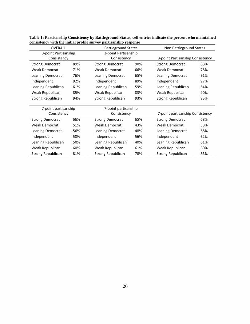
Table 1, offers just such a display based on the CCAP data. The percentages in each cell indicate

the fraction that was always consistent across all waves where they offered a response. The

table is divided with the 3-point measure (Democrat, Independent, and Republican) on top and

the 7-point measure (which includes the weak partisans and the leaning partisans) on the

bottom. The baseline classification is the respondent’s self-classification on the profile

administered at the beginning of the project (i.e., Strong Democrat, Weak Democrat, etc.).6

[Table 1, here]

Looking down the columns, it is generally clear that strong partisans are a bit more

stable than the weak partisans and the leaning partisans. These differences are not always

6 Similar tables could be generated for different standards (i.e., a voter’s response on the final wave. Small differences appear, but the overall pattern remains the same.

13

large. For instance, the strong Republicans are only five percent more likely to be stable in the

non-battleground states. But sometimes the differences are stark: in battleground states, Strong

Democrats are much more likely to be stable than weak Democrats. This certainly pattern is

consistent with all of the perspectives on partisanship, but perhaps fits most closely the idea

from social identity theory that people with stronger identities are more likely to adhere to

those identities.

But as we look across the rows, it is clear that people are, in general, more stable in the

non-battleground states (apparently contradicting the first of our hypotheses). For instance,

only sixty-five percent of “leaning Democrats” in the battleground are perfectly consistent,

compared with ninety-one percent in the non-battleground states. The average increase in

consistency across partisan categories for the 3-point scale is a difference of about nine points—

10 points in the 7-point scale. The table makes clear that the campaign matters, and on the

surface it appears that instability may be related to the campaign.

But, as was stated before, this sort of comparison begs the question of measurement

error. How much of the inconsistency is due to measurement error or to minor deviations from

a person’s standing answer to the partisanship question? To better answer the question we fit a

simple model of partisanship (ϕt) as a function of lagged partisanship (ϕt-1) whether or not a

respondent lived in the battleground (θ) and received a given level of campaign contact (γ).

Because the interest is in discerning the effect of the campaign and the battleground, all of the

terms were interacted (in order to test the interaction hypothesis), and a random effects term

was included for each individual in the sample. See equation (1) for a formal representation of

the model.

14

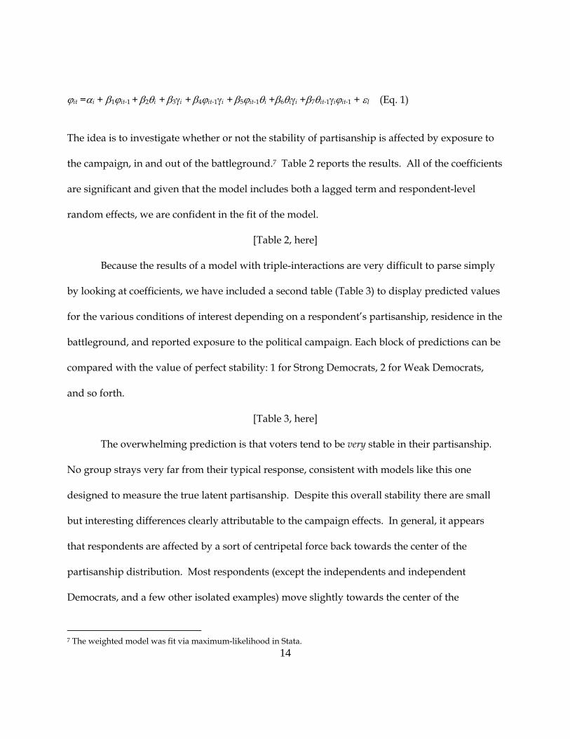
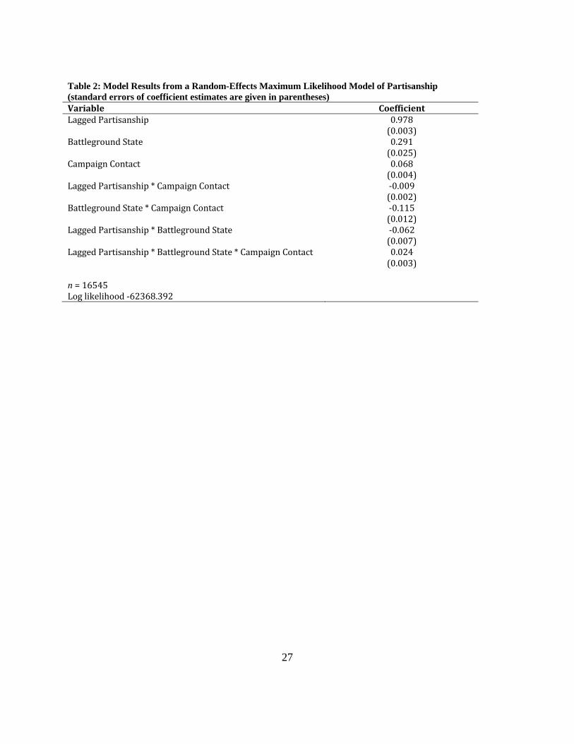
ϕit =αi + β1ϕit-1 + β2θi + β3γi + β4ϕit-1γi + β5ϕit-1θi +β6θiγi +β7θit-1γiϕit-1 + εI (Eq. 1)

The idea is to investigate whether or not the stability of partisanship is affected by exposure to

the campaign, in and out of the battleground.7 Table 2 reports the results. All of the coefficients

are significant and given that the model includes both a lagged term and respondent-level

random effects, we are confident in the fit of the model.

[Table 2, here]

Because the results of a model with triple-interactions are very difficult to parse simply

by looking at coefficients, we have included a second table (Table 3) to display predicted values

for the various conditions of interest depending on a respondent’s partisanship, residence in the

battleground, and reported exposure to the political campaign. Each block of predictions can be

compared with the value of perfect stability: 1 for Strong Democrats, 2 for Weak Democrats,

and so forth.

[Table 3, here]

The overwhelming prediction is that voters tend to be very stable in their partisanship.

No group strays very far from their typical response, consistent with models like this one

designed to measure the true latent partisanship. Despite this overall stability there are small

but interesting differences clearly attributable to the campaign effects. In general, it appears

that respondents are affected by a sort of centripetal force back towards the center of the

partisanship distribution. Most respondents (except the independents and independent

Democrats, and a few other isolated examples) move slightly towards the center of the

7 The weighted model was fit via maximum-likelihood in Stata.

15

distribution (at 4.0). But this centripetal force is not constant. The second column of Table 3

denotes the difference between the hypothesized value (of no movement) and the actual

predicted value generated by the model. The movement ranges from essentially nothing in the

case of several conditions, all the way to a high of .27 in the case of Strong Republicans living in

the battleground states who reported little campaign contact.

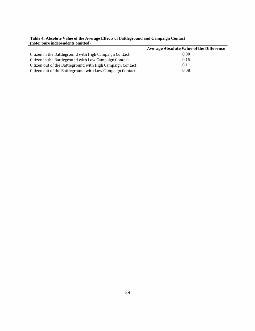
The pattern of effects is probably much easier to see in Table 4, which presents the

average absolute difference by four categories: a citizen living in the battleground with high

campaign contact (i.e., both Republicans and Democrats), a citizen living in the battleground

with low campaign contact, a citizen living outside the battleground with high campaign

contact, and a citizen living outside the battleground with low campaign contact. The results

suggest that in general, there were two groups that were relatively more stable: those living

inside the bubble of heavy-duty campaigning—respondents who resided in the battleground

states and were reporting high campaign contact—and those living completely outside the

bubble—respondents who resided outside the battleground and experienced relatively little

campaign contact.

[Table 4, here]

The results confirm some of our hypotheses but also suggest unanticipated patterns. For

instance, consistent with the interaction hypothesis respondents who were in the battleground,

receiving the strongest campaign messages are the most stable, but this is true only relative to

voters who were receiving some level of campaign attention either because of their residence in

a battleground or by receiving many such messages (presumably some level of choice matters

in the receipt of those messages). The other two hypotheses: residence and campaign volume

16

receive some support, but it appears that relative to the baseline of no immersion in the

campaign these two hypotheses do not receive as much support as we might have expected.

Indeed the two groups that are the most stable are those receiving the strongest messages in the

battleground and those receiving essentially no messages outside of the battleground. We

emphasize that since this model is designed to thwart the possibility of measuring too much

instability the fact that we are finding this much instability that is clearly related to the

campaign is a significant finding. But it does not subvert the overall finding of stability.

When Zaller writes (admittedly in a very different context) that “public opinion can be

understood as a response to the relative intensity and stability of opposing flows of …

communications (Zaller 1992, p. 186)” he seems to be describing a phenomenon that applies to

partisan attitudes. In the most intense flow of information, respondents were extremely stable.

The other place they were extremely stable was in the environment completely lacking in

intensity. Put voters in between these two extremes and they appear to become somewhat

more unstable—moving in some cases, on average, as much as a quarter of the way towards a

more centrist category.

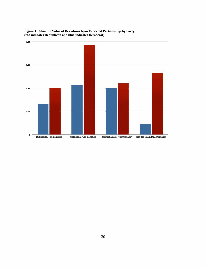
But this overall pattern masks some partisan patterns to the instability that can be seen

in Figure 1 that divides the average absolute instability by partisanship. Republicans are

always more likely to be unstable—Republicans living in the battleground, but not getting the

reinforcement of high campaign contact moving an average of almost 20 percent towards the

category of “Weak Republican.” To us this seems like a feature of the 2008 campaign where

Obama was remarkably popular and clearly maintained the upper hand in the campaign almost

through the general election contest (and much of the primary as well).

17

[Figure 1, here]

Taken on balance we see three simple lessons from the data. First, partisanship is

generally quite stable. It is not the case that any group here is making wild shifts: people are

clearly stable, on average. But, second, there is some instability that must be linked to the

campaign. Given that much of the campaign is accounted for in the model by simple residence

in our out of the battleground, we would argue that there is clearly a causal mechanism at work

here. Direct causality is muddied by the fact that the model also includes a measure of reported

campaign contact. Although we believe that this measure is a good proxy for actual exposure

to the campaign.8 This means that others who have written about the magic of the battleground

are right. Partisanship—perhaps the most ubiquitous concepts in American politics and

certainly a concept that everyone regards as one of the most stable attitudes possible—is clearly

affected by the campaign experienced by a voter.

Finally, we would point out that this model is evidence that not only the specific

campaign tactics matter (contacts, advertising, etc.), but so do the fundamentals. The

Republicans began 2008 in a deep hole because of the fundamentals of the race. An unpopular

president, his foreign adventures, and an incredibly poor economy all combined to create a

situation where much more of the instability that appears in the data came among Republicans

rather than among Democrats.

8 At least it was the best that we could locate within the CCAP data.

18

5. Discussion

The model results broadly support some of our expectations: not all inconsistency is

created equal. Some partisanship instability is measurement error in the sense of miscoding or

simple mistakes. But some of it is clearly related to campaign environment and volume for a

specific voter.

These results do suggest that partisanship—while it may be a social-psychological

identity—is partially the result of interactions with the political environment, particularly the

short-run environment of intensive campaigning. This makes sense. Individuals who construct

a social identity do so in a given context. That context can either reinforce or undermine the

identity and can present the individual with new questions, or perhaps even new dimensions,

about that identity. This seems to be the dynamic element of a model of social-psychological

identity. It is also thoroughly consistent with models of electoral change that specify the ways

in which voters “update” preferences given party performance.

When political scientists measure partisanship, they typically rely on the simple

question “Generally speaking, do you consider yourself a Republican, a Democrat, an

Independent, or something else?” As revealing as this question is, it does not directly tap the

ambivalence and uncertainty that potentially lies underneath the surface for some citizens. And

it certainly does not tap dimensions that would tend to strengthen or weaken identities.

Someone may say that they are a Republican simply because they feel closer to that party than

the other party. Change the electoral conditions or present that individual with the right

campaign message and he might well have the identity positively or negatively reinforced.

Indeed campaigns, while they are obviously designed to win votes, are the perfect environment

19

in which to test a person’s commitment. Maybe he identifies as a Democrat, but is he so

committed to the identity that he will never allow conflicting messages or images to question a

commitment to that identity?

We believe this work simply scratches the surface of the issue. Some of the work that has

been done on “certainty” of votes should probably be done on certainty of partisanship.

Alternative questions wording would also be helpful. Lastly, the interesting effects of different

campaign media suggests the need for experimental work on types of campaign messages that

reinforce partisan identities.

Political science has treated “partisanship” too simply. Like any other attitude held by

fallible human beings, it is not something unaffected by the institutional context. Voters can be

conflicted—sometimes for very good reasons like the fact that they can disagree with other

members of their party on some key issue, sometimes simply because of the campaign context.

Voters are sometimes unaware of conflicts between their opinions and their partisanship and

only the campaign arena is likely to highlight that problem. Furthermore, even though

partisanship could be considered a social identity, rising or declining fortunes of a party (such

as the Republicans experienced in 2008) may make individuals more or less likely to cling so

tenaciously to those identities.

Partisanship stability is clearly what we should expect out of the voter, but only under

the right conditions. Most of the time voters are already correctly sorted into parties and

comfortable with their identity. New issues or dramatic elections that can upset that applecart

do not come along every day. In a political environment where individuals have ready access

to political information and cues, we might see partisan stability as the typical case. This means

20

that the observed stability of partisanship may be, in part, an artifact of the nature of our party

system where some candidates vigorously contest some jurisdictions and virtually ignore

others, thus maximizing the chances of stability for some individuals, but minimizing it for

others.

21

Appendix: Question Wording and Variable Coding Party Identification Generally speaking, do you think of yourself as a…Democrat, Republican, Independent, Other, Not Sure” Respondents answering “Republican” or “Democrat” were asked: “Would you call yourself a strong [Republican/Democrat] or a not very strong [Republican/Democrat]?” Respondents answering “Independent,” “Other,” or “Not Sure” were asked: “Do you think of yourself as closer to the Democratic or the Republican Party?” We used the full seven point party identification scale from each wave of the panel. Respondents answering “not sure” a second time to the “leaner” question were reclassified as “pure independents” (4) on the seven point scale. Battleground States The battleground state variable was coded using a list of eighteen states considered by the Obama campaign to be major battlegrounds as of June 2008. See: http://www.fivethirtyeight.com/2008/06/obama-eighteen.html. The eighteen states are: Alaska, Colorado, Florida, Georgia, Indiana, Iowa, Michigan, Missouri, Montana, Nevada, New Hampshire, New Mexico, North Carolina, North Dakota, Ohio, Pennsylvania, Virginia, and Wisconsin. Most of these states are familiar to recent presidential contests and/or other lists of 2008 battleground states and thus the list has tremendous face validity. There are a few unusual states on the list, but these unfamiliar battlegrounds such as Alaska, Montana, and North Dakota have small populations and are thus do not make up a large proportion of the survey respondents. Their presence or absence in the battleground list does not appreciably affect our results. Campaign Contact Thinking about the presidential candidates and their campaigns, did any of the following things happen to you YESTERDAY? (Choose as many as apply) <1> Saw a campaign ad on TV <2> Received a piece of campaign mail (US Post or email) <3> Donated money to a candidate or party <4> Received a pamphlet on my door <5> Wore a button or sticker for a candidate <6> Discussed a candidate with someone <7> Received a visit from a campaign worker <8> Heard a radio ad for a candidate <9> Saw a yard sign for a candidate <10> Went to hear a candidate speak

22

<11> Got a phone call from a campaign <12> Visited a candidate web site <13> Heard about candidate at religious service <14> Watched video of candidate on Internet [September and October waves only] We summed the contacts for each of the five pre-election campaign waves. The resulting index is right skewed and so we took the natural log of the index and included both in the model and used the log of campaign contact to create the interaction terms.

23

References

Allsop, Dee and Herbert F. Weisberg. 1988. “Measuring Change in Party Identification in an Election Campaign.” American Journal of Political Science 32: 996-1017.

Berelson, Bernard R., Paul F. Lazarsfeld, and William N. McPhee. 1954. Voting. Chicago:

University of Chicago Press. Bowler, Shaun, David J. Lanoue, and Paul Savoie. 1994. “Electoral Systems, Party Competition,

and Strength of Partisan Attachment: Evidence from Three Countries.” The Journal of Politics 56: 991-1007.

Brody, Richard A. and Lawrence S. Rothenberg. 1988. “The Instability of Partisanship: An

Analysis of the 1980 Presidential Election.” British Journal of Political Science 18: 445-65. Cambell, Angus, Phillip E. Converse, Warren E. Miller, and Donald E. Stokes. 1960. The

American Voter. New York: John Wiley and Sons. Downs, Anthony. 1957. An Economic Theory of Democracy. New York: Harper & Row. Erikson, Robert S, Michael B. Mackuen, and James A. Stimson. 1989 “Macropartisanship.” The

American Political Science Review 83: 1125-1142 Erikson, Robert S, Michael B. Mackuen, and James A. Stimson. 1998. “What Moves Macropartisanship?

A Response to Green, Palmquist, and Schickler.” The American Political Science Review 92: 901-912

Finkel, Steven. 1993. “Reexamining the “Minimal Effects” Model in Recent Presidential

Campaigns.” The Journal of Politics 55: 1-21. Finkel, Steven E. and Howard A Scarrow. 1985. “Party Identification and Party Enrollment:

The Difference and the Consequences.” The Journal of Politics 47: 620-642. Fiorina, Morris P. 1981. Retrospective Voting in American National Elections. New Haven: Yale

University Press. Franklin, Charles, F. 1992. “Measurement and the Dynamics of Party Identification.” Political

Behavior 14: 297-309. Franklin, Charles F., and John E. Jackson. 1983. “The Dynamics of Party Identification.”

American Political Science Review 77: 957-973. Freedman, Paul, Michael Franz, and Kenneth Goldstein. 2004. “Campaign Advertising and

Democratic Citizenship.” American Journal of Political Science 48:723-41.

24

Gelman, Andrew and Gary King. 1993. “Why are American Presidential Election Campaign Polls so Variable When Votes are so Predictable?” British Journal of Political Science 23:409-501.

Gimpel, James G., Karen M. Kaufman, and Shanna Pearson-Merkowitz. 2007. “Battleground

States versus Blackout States: The Behavioral Implications of Modern Presidential Campaigns.” Journal of Politics 69: 786-797.

Green, Donald P. and Alan S. Gerber. 2004. Get Out the Vote! How to Increase Voter Turnout.

Washington D.C.: Brookings Institution Press. Green, Donald P. and Alan S. Gerber, eds. 2005. The Science of Voter Mobilization. The Annals of

the American Academy of Political and Social Science, Vol. 601. Thousand Oaks, CA: Sage Publications.

Green, Donald, and Bradley Palmquist. 1990. “Of Artifacts and Partisan Instability.” American

Journal of Political Science 34: 872-902. Green, Donald, Bradley Palmquist, and Eric Schickler. 2002. Partisan Hearts and Minds. New

Haven: Yale University Press. Greene, Steven. 2004. “Social Identity Theory and Party Identification.” Social Science Quarterly

85: 136-153. Gronke, Paul. 2000. The Electorate, the Campaign and the Office. Ann Arbor: University of

Michigan Press. Hillygus, Sunshine, and Simon Jackman. 2003. “Voter Decision Making in Election 2000:

Campaign Effects, Partisan Activation, and the Clinton Legacy.” American Journal of Political Science 47:583-96.

Hillygus, Sunshine, and J. Quin Monson. 2008. “The Ground Campaign: The Strategy and

Influence of Direct Communications in the 2004 Presidential Election.” Unpublished paper.

Hogg, Michael A, Deborah J. Terry, and Katherine M. White. 1995. “A Tale of Two Theories: A

Critical Comparison of Identity Theory with Social Identity Theory.” Social Psychology Quarterly 58: 255-269.

Jackman, Simon and Lynn Vavreck. 2009a. “The Magic of the Battleground: Uncertainty,

Learning, and Changing Information Environments in the 2008 Presidential Campaign.” Paper prepared for presentation at the UCSD Seminar, May 16, 2009.

25

------------. 2009b. Cooperative Campaign Analysis Project, 2007-2008 Panel Study. Common Content Codebook, Advance Release 1.0.

------------. 2009c. Constructing the 2007-2008 Cooperative Campaign Analysis Project Sample.

Unpublished paper. Lazarsfeld, Paul, Bernard Berelson, and Hazel Gaudet. 1944. The People’s Choice: How the Voter

Makes Up His Mind in a Presidential Campaign. New York: Columbia University Press. Miller, Warren E. 1991. “Party Identification, Realignment, and Party Voting: Back to the

Basics” American Political Science Review 85: 557-68. McClurg, Scott D. and Thomas M. Holbrook. 2009. “Living in a Battleground: Presidential

Campaigns and Fundamental Predictors of Vote Choice.” Political Research Quarterly 62: 495-506.

Niemi, Richard G, David R. Reed, and Herbert F. Weisberg. 1991. “Partisan Commitment: A

Research Note.” Political Behavior 13: 213-221. Page, Benjamin I. and Calvin C. Jones. 1979. “Reciprocal Effects of Policy Preferences, Party

Loyalty, and the Vote.” American Political Science Review 73: 1071-90. Shaw, Daron R. 1999. “The Methods behind the Madness: Presidential Electoral College

Strategies, 1988-1996.” Journal of Politics 61: 893-913. --------. 2006. The Race to 270: The Electoral College and the Campaign Strategies of 2000 and 2004.

Chicago: University of Chicago Press. Stets, Jan E, and Peter J. Burke. 2000. “Identity theory and Social Identity Theory.” Social

Psychology Quarterly 63: 224-237. Vavreck, Lynn and Douglas Rivers. 2008. “The 2006 Cooperative Congressional Election Study”

Journal of Elections, Public Opinion & Parties 18:355-66. Wolak, Jennifer. 2006. “The Consequences of Presidential Battleground Strategies for Citizen

Engagement.” Political Research Quarterly 59: 353-361 Zaller, Jonathan. 1992. The Nature and Origins of Mass Opinion. Cambridge University Press.

26

Table 1: Partisanship Consistency by Battleground Status, cell entries indicate the percent who maintained consistency with the initial profile survey partisanship response

OVERALL    Battleground States    Non Battleground States 3‐point Partisanship 

Consistency   3‐point Partisanship 

Consistency    3‐point Partisanship Consistency 

Strong Democrat  89%       Strong Democrat  90%       Strong Democrat     88%    Weak Democrat  71%       Weak Democrat  66%       Weak Democrat     78%    Leaning Democrat  76%       Leaning Democrat  65%       Leaning Democrat     91%    Independent  92%       Independent  89%       Independent     97%    Leaning Republican  61%       Leaning Republican  59%       Leaning Republican     64%    Weak Republican  85%       Weak Republican  83%       Weak Republican     90%    Strong Republican  94%       Strong Republican  93%       Strong Republican     95%                 

7‐point partisanship Consistency   

7‐point partisanship Consistency    7‐point partisanship Consistency 

Strong Democrat  66%       Strong Democrat  65%       Strong Democrat     68%    Weak Democrat  51%       Weak Democrat  43%       Weak Democrat     58%    Leaning Democrat  56%       Leaning Democrat  48%       Leaning Democrat     68%    Independent  58%       Independent  56%       Independent     62%    Leaning Republican  50%       Leaning Republican  40%       Leaning Republican     61%    Weak Republican  60%       Weak Republican  61%       Weak Republican     60%    Strong Republican  81%       Strong Republican  78%       Strong Republican     83%    

27

Table 2: Model Results from a Random-Effects Maximum Likelihood Model of Partisanship (standard errors of coefficient estimates are given in parentheses) Variable  Coefficient  Lagged Partisanship  0.978   (0.003) Battleground State  0.291   (0.025) Campaign Contact  0.068   (0.004) Lagged Partisanship * Campaign Contact  ‐0.009   (0.002) Battleground State * Campaign Contact  ‐0.115   (0.012) Lagged Partisanship * Battleground State ‐0.062   (0.007) Lagged Partisanship * Battleground State * Campaign Contact  0.024   (0.003)  n = 16545  Log likelihood ‐62368.392 

28

Table 3: Predicted Partisanship and Difference From Hypothesized Value, note: bolded coefficients indicate statistical significance at p < 0.05

Partisan / Battleground / Campaign Status  Partisan Estimate 

Difference from 

Hypothesized Stability Value 

Strong Democrat in a battleground with high campaign contact 1.11  ­0.11 Strong Democrat in a battleground with little campaign contact 1.18  ­0.18 Strong Democrat not in a battleground with high campaign contact 1.15  ­0.15 Strong Democrat not in a battleground with low campaign contact 1.02  ‐0.02      Weak Democrat in a battleground with high campaign contact 2.07  ­0.07 Weak Democrat in a battleground with little campaign contact 2.11  ­0.11 Weak Democrat not in a battleground with high campaign contact 2.10  ­0.10 Weak Democrat not in a battleground with low campaign contact 1.99  0.01      Independent Democrat in a battleground with high campaign contact 3.03  ‐0.02 Independent Democrat in a battleground with little campaign contact 3.03  ‐0.03 Independent Democrat not in a battleground with high campaign contact  3.05  ­0.05 Independent Democrat not in a battleground with low campaign contact  2.96  0.04      Independent in a battleground with high campaign contact 3.98  0.02 Independent in a battleground with little campaign contact 3.96  0.04 Independent not in a battleground with high campaign contact 4.00  0.00 Independent not in a battleground with low campaign contact 3.93  0.07      Independent Republican in a battleground with high campaign contact 4.94  0.06 Independent Republican in a battleground with little campaign contact 4.88  0.12 Independent Republican not in a battleground with high campaign contact  4.95  0.05 Independent Republican not in a battleground with low campaign contact  4.90  0.10      Weak Republican in a battleground with high campaign contact 5.90  0.10 Weak Republican in a battleground with little campaign contact 5.81  0.19 Weak Republican not in a battleground with high campaign contact 5.87  0.13 Weak Republican not in a battleground with low campaign contact 5.87  0.14      Weak Republican in a battleground with high campaign contact 6.86  0.14 Weak Republican in a battleground with little campaign contact 6.74  0.27 Weak Republican not in a battleground with high campaign contact 6.85  0.15 Weak Republican not in a battleground with low campaign contact 6.84  0.16 

29

Table 4: Absolute Value of the Average Effects of Battleground and Campaign Contact (note: pure independents omitted)   Average Absolute Value of the Difference Citizen in the Battleground with High Campaign Contact  0.08 Citizen in the Battleground with Low Campaign Contact  0.15 Citizen out of the Battleground with High Campaign Contact  0.11 Citizen out of the Battleground with Low Campaign Contact  0.08 

30

Figure 1: Absolute Value of Deviations from Expected Partisanship by Party (red indicates Republican and blue indicates Democrat)