The Bush Tax Cut and National Saving

The Bush Tax Cut and National Saving

Alan J. AuerbachUniversity of California, Berkeley and NBER

June 2002

This paper was prepared for the May, 2002, Spring Symposium of the National Tax Associationin Washington DC. I am extremely grateful to Dan Feenberg for producing and helping tointerpret marginal tax rate estimates from the NBER TAXSIM model and to Bill Gale, KevinHassett, Kent Smetters, and participants in the Canadian Public Economics Study Group forcomments on previous drafts.

Abstract

Following through on pledges made during his election campaign, President Bush

proposed and Congress passed a substantial tax cut in 2001, the Economic Growth and Tax

Relief Reconciliation Act (EGTRRA). Much has been written about the size of the tax cut, its

impact on the federal budget, its distributional consequences, and its short-run macroeconomic

impact. There has been less focus on EGTRRA’s incentive effects; one of the most important

potential behavioral effects is on saving.

To analyze the behavioral effects of the Bush tax cut on saving and other macroeconomic

variables, I use the Auerbach-Kotlikoff (1987) model in conjunction with the NBER’s TAXSIM

model. An interesting by-product of this analysis is the “dynamic scoring” of the tax cut – the

estimated feedback effects of behavior on revenue. By comparing the revenue losses generated

by the model with those that would occur without any behavioral response, one can estimate how

much of the static revenue loss would be recouped by expanded economic activity. The

simulations suggest that dynamic scoring has a significant impact on estimated revenue losses,

but that the tax cut’s impact on national saving is still negative in the long run.

Alan J. AuerbachDepartment of EconomicsUniversity of California549 Evans HallBerkeley, CA [email protected] JEL Nos. E62, D91

INTRODUCTION

Following through on pledges made during his election campaign, President Bush

proposed and Congress passed for his signature a substantial tax cut in 2001, forever linked to

the unwieldy acronym EGTRRA (the Economic Growth and Tax Relief Reconciliation Act).

Much has been written about the size of the tax cut, its impact on the federal budget, and its

distributional consequences. There has also been considerable debate over the politics and

economics of the tax cut’s “unfinished business.” These include, in particular, the growing

problem of the Alternative Minimum Tax (AMT), which was exacerbated by EGTRRA’s

reduction in ordinary income tax burdens, and the tax cut’s “sunset” after 2010. The tax cut’s

passage has also prompted a debate about its short-run macroeconomic consequences, with

respect to both its timing and whether its “back-loaded” structure undercut its ability to spur

economic activity during the recent economic downturn.

Throughout this debate, there has been less focus on EGTRRA’s incentive effects. This

lack of attention might be surprising, given that the lion’s share of the projected revenue losses

come from reductions in statutory marginal tax rates and through other provisions (such as the

phasing out of the estate tax) that would be expected to influence behavioral incentives. The

focus on other issues may relate to the complexity of the legislation, the various phase-ins and

phase-outs, and the difficulty of modeling the simultaneous effects of such a large number of

provisions. Yet, an important underlying motivation for many in pursuing this tax cut was the

notion that lower taxes can spur private activity and thereby make the economy more productive.

It seems, then, that efforts to evaluate the tax cut’s incentive effects are important, if challenging.

One of the most important potential behavioral effects is on saving, which affects future

productivity and living standards through capital deepening.

2

This paper focuses on the net national saving rate as a summary measure of the nation’s

rate of capital accumulation. The net national saving rate is the share of net output that is

consumed by neither government nor households. Unlike measures of saving based on the

behavior of the private sector or households alone, the net national saving rate accounts for

government saving and therefore is a comprehensive measure of the share of output put aside by

the economy as a whole for capital accumulation. This inclusion of government saving is

especially important in analyzing policies, such as tax cuts, under which resources are being

shifted from government to the private sector, because private and personal saving rates may rise

even as national saving falls.

To analyze the behavioral effects of the Bush tax cut, I use the Auerbach-Kotlikoff (1987,

hereafter AK) model, a dynamic general equilibrium simulation model that incorporates the

behavior of firms, government and forward-looking households. The AK model has been used

extensively over the years to evaluate fundamental tax reforms, such as replacing the federal

income tax with a consumption tax, but it is also capable of measuring the effects of more

incremental changes in the tax system like those adopted in 2001.

The remainder of the paper is organized as follows. The next section describes the major

provisions of EGTRRA that will be evaluated, indicating their impact on marginal tax rates and

their potential effects on behavior. The following section describes the AK model and how the

model is used to study the effects of the tax cut. The remainder of the paper presents simulation

results of the effects of the tax cut on saving and output under a variety of assumptions. The

simulations suggest that the Bush tax cut may increase saving in the short run, depending on

assumptions, and that it is likely to increase output in the short run, due to its additional salutary

effects on labor supply. In the longer run, though, saving and output are likely to fall, once the

3

revenue losses generated by the tax cut are confronted through necessary policy changes. Only if

the revenue losses are entirely offset by reductions in government consumption spending can this

long-run outcome be avoided. Thus, whatever its benefits, the tax cut does not offer the promise

of enhancing saving and expanding output in the long run.

An interesting by-product of this analysis is the “dynamic scoring” of the tax cut – the

estimated feedback effects of behavior on revenue. By comparing the revenue losses generated

by the model with those that would occur without any behavioral response, one can estimate how

much of the static revenue loss would be recouped by expanded economic activity. Although the

AK model is well suited for such calculations, it has not been used for this purpose in the past.

The results below suggest that static revenue estimates generally overstate the net revenue loss

from tax cuts like EGTRRA, even for simulations in which the tax cuts are projected to reduce

national saving and output. That is, the results regarding saving and output summarized above

take place in spite of the recoupment of revenue predicted by the model.

EGTRRA: PROVISIONS AND EFFECTS

While EGTRRA contained many provisions, the most important from the perspective of

revenue cost were those reducing marginal income tax rates. These included the creation of the

new 10 percent bracket in 2001 below the 15 percent bracket and the phase in of lower marginal

tax rates in higher brackets. The legislation would further reduce effective marginal tax rates

through the phased repeal of the itemized deduction and personal exemption phase-outs. Under

the heading of “marriage penalty relief,” the legislation broadens the 15 percent bracket and

reforms the Earned Income Tax Credit for married couples, both provisions that reduce marginal

tax rates for some taxpayers.

4

These rate reductions were accompanied by an increase in the child tax credit and (for

couples) the standard deduction, provisions that could, indirectly, reduce marginal tax rates

slightly by sheltering more income from tax. There was also a temporary provision (through

2004) to increase the AMT exemption level, aimed at reducing the number of additional

taxpayers subject to the AMT because of the other provisions.

When EGTRRA became law, the Joint Committee on Taxation (JCT 2001) estimated that

the provisions listed above accounted for 82 percent of its revenue loss in 2010, the last full year

of the tax cut prior to its legislated sunset, and 87 percent over the period 2001-2010.1 This

paper considers the macroeconomic effects of these provisions, as a group.

The most significant element omitted from this list of provisions is the phased repeal of

the estate tax, which accounts for about half of the remaining revenue loss between 2001 and

2010. There are two reasons for this omission. First, there is considerable uncertainty about

how to model the effects of the estate tax on behavior (see, e.g., the collection of papers in Gale,

Hines and Slemrod, 2001). While bequests appear sensitive to estate tax rates, the motivations

for bequest saving and the manner in which taxes influence estate planning are not clear. Thus,

there would be enormous uncertainty attached to any particular modeling assumptions. Second,

the results based on any given behavioral specification will also be very sensitive to one’s

assumption about the permanence of estate tax repeal. Under the law as passed, estate tax repeal

lasts for just one year, 2010, after which the pre-2001 rules apply. If this law remains in force,

estate tax repeal is likely to have very insignificant effects on saving. On the other hand, if estate

tax repeal is extended for a significant period of time, then its impact could be more important,

5

depending then on the particular behavioral assumptions one chose.2 Thus, the analysis of this

paper and its conclusions apply to the Bush tax cut, excluding changes in the estate tax.

Impact of EGTRRA on Marginal Tax Rates

Table 1 presents estimates of the effects of EGTRRA on average marginal tax rates

(weighted by the respective type of income) faced by labor income, interest and dividend

income, and long-term capital gains for each year during the period 2001-2010.3 All calculations

are based on a 1996 sample of tax returns, with later years simulated using the assumption of

smooth growth in prices (3 percent per year), population (1.2 percent per year) and real per

capita income (1 percent per year). The table’s first three columns project tax rates that would

have prevailed had EGTRRA not been enacted. Even with no change in law, average marginal

tax rates would have risen through “real” bracket creep, the migration of taxpayers into higher

brackets due to real income growth.

With EGTRRA in effect, marginal rates are lower, progressively more so until 2006,

when most of the main provisions are phased in. Two patterns regarding capital income taxes

are worth noting. First, the reductions in average marginal tax rates on interest and dividend

income are higher than those on wage and salary income because interest and dividend income

are more concentrated in higher brackets that eventually enjoy a larger percentage-point drop in

1 The JCT estimates for these provisions total $152.8 billion in 2010, compared to an overall revenue loss of $187.0billion. For the period 2001-2010, the comparable figures are $1,054.7 billion and $1,219.0 billion, respectively.The percentages for other individual years are similar, except for 2001 (when the percentage is lower) and 2002(when it is higher). These exceptions are attributable to a large shift in corporate estimated taxes from 2001 to 2002adopted solely to push more revenue into the relevant budget window.2 As discussed below, the impact of all provisions depends to some extent on the assumed permanence of the tax cut.But the nature of the estate tax, with its very long planning horizon and large one-time tax assessment, makes thisissue much more important.3 The estimates in Table 1 of reductions in marginal tax rates on wages and interest and dividend income aresomewhat higher than those estimated by Treasury and CBO, summarized in Gale and Potter (2002), Table 6. Tothe extent that the figures used here overstate the marginal rate reductions, they are also likely to overstate the taxcut’s salutary effects.

6

marginal tax rates. Second, the average marginal tax rate on long-term capital gains is actually

slightly higher under EGTRRA. The primary reason for this involves the AMT.

As discussed above, EGTRRA pushes more taxpayers onto the AMT. At first, one might

think that this would have no impact on the tax rate faced by capital gains, for the 20 percent

maximum capital gains tax rate applies under both the ordinary income tax and the AMT. But

the AMT contains a provision that phases out the initial exemption amount. This provision

works much like the personal exemption and itemized deduction phase-outs under the ordinary

income tax, but it has a much more powerful effect on marginal tax rates, because the AMT

exemption is large and the rate of phase-out is high.

In 2001, joint filers on the AMT with incomes between $150,000 and $346,000 lost 25

cents of exemptions for each added dollar of income (including capital gains). This had the

effect of raising the marginal tax rate on income within this broad range by one-fourth of the

statutory AMT marginal tax rate, which was 28 percent for most affected taxpayers. Hence, a

dollar of capital gain income was subject to a marginal tax rate of 27 percent (20 + .25 x 28), not

20 percent. With more taxpayers pushed onto the AMT, capital gains are potentially subject to

much higher marginal tax rates. It is doubtful that President Bush intended to increase capital

gains taxes, but this is one result of his plan.

SIMULATING THE IMPACT OF EGTRRA ON BEHAVIOR

Simulating the effects of EGTRRA with the AK model requires a variety of adjustments

to the data in Table 1 and some additional calculations and assumptions.

First, I adjust revenues in the model to track the revenue losses projected by the Joint

Committee on Taxation, using contemporaneous projections of fiscal-year output by the

Congressional Budget Office (2001) to estimate annual revenue losses as a share of output. I

7

treat the JCT’s projections as being “static” revenue estimates4 and calibrate the model so that its

static revenue losses as a share of output match these revenue estimates, which are shown in the

last column of Table 1.5 Note that these revenue losses will not correspond to those in the

model’s full simulations, because of dynamic revenue feedback effects.

Second, I take the year 2001 tax system, pre-EGTRRA, as the baseline, and consider the

impact on this baseline of the tax rate changes given in the third panel of Table 1. Thus, I ignore

the underlying drift in marginal tax rates that would have occurred without EGTRRA, and apply

the changes in marginal tax rates to the 2001 baseline.

Third, to reduce the complexity of the simulations, I assume that there are a small number

of tax regimes under EGTRRA, even though phase-outs and phase-ins make the provisions in

effect in each year somewhat distinct from those in adjoining years. Based on the numbers in

Table 1, it involves minimal approximation error to assume that there are four tax regimes under

EGTRRA, for the years 2001, 2002-3, 2004-5, and 2006-10, and to use for each regime averages

of the tax rates and revenue losses in the years of the regime. The marginal tax rates for these

regimes are given in the first three columns of Table 2. The last column of Table 2 lists the

target ratio of revenue to NNP, based on the revenue losses in Table 1 and an assumed initial

ratio of 15.0 percent. This ratio equals the share of federal revenues, excluding payroll taxes,

which are treated separately in the model. The baseline value is set at 15.0 percent, slightly

higher than the actual 2001 value, to take account of the impact of the tax cut.

4 The JCT’s revenue estimates are not fully static, because they incorporate behavioral changes at the micro level.For example, they allow for taxpayer responses to changes in capital gains tax rates, but not the macro feedbackeffects of changes in aggregate output. See Auerbach (1996a) for further discussion. It would be preferable to usetruly static revenue estimates for this calibration exercise, but these are not publicly available. The paper’s estimatesof dynamic feedback effects would not be significantly affected, however, because they depend on the differencebetween the assumed static revenue loss and the revenue loss projected by the model.5 Because output in the model is net of depreciation, the output measure used to calculate revenue shares is netnational product (NNP), estimated by adjusting CBO’s 2001-2010 GDP projections by the 2000 NNP-GDP ratio.

8

Fourth, it is necessary to adjust taxes on labor income to account for the fact that taxes on

some compensation are deferred. One must also adjust capital income taxes, to reflect both

additional taxes at the corporate level and the fact that substantial shares of capital income are

received in tax-sheltered forms. These adjustments are complex, and so the details of how they

are carried out are relegated to the Appendix. The methodology closely follows that developed

in Auerbach (1996b) but is based on more recent data. Table 3 provides the tax rates that result

from these calculations. The first column lists the average tax rate on wages, set as a residual to

hit the target revenue level given in Table 2. The second column lists the marginal tax rate on

wage income that, when combined with the consumption tax rate in the next column, yields a full

effective marginal tax rate on wages equal to the corresponding value in Table 2. The third

column lists the consumption tax rate, which is used (as discussed in the Appendix) to account

for the deferred taxes on sheltered compensation. The fourth column lists the capital income tax

rate, derived according to the methodology that is described in the Appendix.

Parameterizing the AK Model

The paper uses the AK model to simulate the macroeconomic effects of tax changes. This

is a dynamic model that, at each date, has 55 overlapping generations of individuals who save

and supply labor to maximize a nested CES lifetime utility function.6 There is a single

production sector and a government sector with two functions, one a pay-as-you-go social

insurance system and the other encompassing all remaining federal government activities. This

general government sector imposes taxes on consumption, capital income, and labor income.

The labor income tax is specified as a quadratic function of income, thus allowing the marginal

9

and average income tax rates to differ. By adjusting the two parameters of the labor income tax

function, one can hit both a revenue target and a desired average marginal tax rate.

All of the simulations presented below preserve a number of the original assumptions in

Auerbach and Kotlikoff (1987) and in Auerbach (1996b). These assumptions include a

population growth rate of 1.5 percent per year, a Cobb-Douglas production function, a relative

weight of 1.5 for leisure in each period’s utility sub-function of leisure and consumption, and a

perceived offset of .25 of payroll taxes in terms of perceived future benefits. Unless otherwise

reported, all simulations also follow the original assumptions regarding the pure rate of time

preference (1.5 percent per year), the intertemporal elasticity of substitution (0.25), and the

intratemporal elasticity of substitution between leisure and goods (0.8). Reflecting the need to

consider realistic short-run responses to tax cuts, I incorporate investment adjustment costs,

following the parameterization used for such simulations in Auerbach (1996b).7 Except where

noted, simulations assume a closed economy.

The initial steady state is calibrated so that the payroll tax rate is 15.3 percent, the sum at

present of employer and employee contribution rates. The initial level of the national debt equals

40 percent of NNP, roughly its value at the end of 2000. As discussed above, the average tax

rate on labor income is adjusted to ensure that the revenue from the non-social-insurance

government sector is 15 percent of output, the latter corresponding in the model to NNP.

6 The version used here ignores the bequest motive, except where noted. Recent simulations by Altig et al. (2001)using an extension of the AK model suggest that incorporating the bequest motive does not have a major impact onthe estimated effects of major tax reforms on output and capital accumulation. (The reforms considered did notinvolve the estate tax.)7 In the model the quadratic adjustment cost parameter is set so that an increase of 1 percentage point in theinvestment-capital ratio increases the cost of investment goods by 10 percent. As discussed in Auerbach (1996b),this is a reasonable estimate, based on the literature. It also corresponds to the base case used by Altig et al. (2001).

10

Modeling Tax Cuts

As discussed above, EGTRRA includes a phase in of provisions through 2010, followed

by a sunset in 2011. This sunset is duly incorporated by the JCT in its revenue estimates, as

required, but it is not necessarily consistent with expectations. To simulate the effects of

EGTRRA, expectations must be taken into account. In the forward-looking behavior of the

agents in the AK model, decisions about labor supply and saving during the legislated period of

the tax cut depend on what agents believe about the tax cut in the years after 2010. Thus, a

complete simulation must specify the full path of fiscal policy, not just its path through 2010.

Given our uncertainty about what actually will happen, I provide simulations corresponding to a

number of alternative assumptions about post-2010 fiscal policy.

While each of these alternative scenarios may be realistic, none correspond to the

apparently simple and appealing assumption that the tax cut will be permanent. Without some

further adjustment, this assumption would be meaningless, assuming that fiscal policy was on a

feasible trajectory to begin with, for it would specify an infeasible fiscal policy path of exploding

national debt. It is an even more unreasonable assumption in the current environment, in which a

sizable fiscal gap would exist under current policy even had EGTRRA not been implemented

(Auerbach, Gale and Orszag 2002).

To separate the analysis below from a more general consideration of how to close the

preexisting fiscal gap, all simulations assume (optimistically) that pre-EGTRRA fiscal policy

was just sustainable, and that, eventually, the revenue losses introduced by EGTRRA must be

offset by fiscal adjustments. In the short run, these adjustments can be deferred by accumulating

federal debt, but at some date, which varies by simulation, it is assumed that the per capita level

11

of debt is stabilized by a tax rate adjustment. The simulations also differ according to which tax

rate is assumed to adjust at this date of reckoning.

BASIC RESULTS

The AK model traces the path of the economy starting from an initial steady state, here

taken to be the year 2000, through a period of 150 years, at which time the economy is assumed

to have converged to a new steady state. Thus, results for the year 2150 correspond to those for

the “long run” after all aggregates in the model have stabilized.

Initially, I consider five simulations, differing by how long EGTRRA is assumed to last

and the compensating fiscal instrument that is adjusted after its repeal. These simulations are

labeled w10, k10, w15, k15, and k20. The prefix w indicates that the proportional component of

the wage tax function is adjusted after the tax cut is repealed; the prefix k indicates that the

capital income tax serves this residual purpose.8 The suffixes 10, 15, and 20 indicate the number

of years the tax cut is assumed to stay in place, from the originally legislated 10 years to a period

twice this length. For simulations in which the tax cut lasts longer than currently legislated, I

assume that the tax rates from the 2006-2010 regime continue to apply. For all simulations, I

assume that debt accumulates while the tax cut is in place, and is stabilized in per capita terms

thereafter. Because tax cuts lead to higher debt levels, the eventual stabilization of debt requires

an increase in the residual tax component (w or k) above its pre-tax-cut value.

8A 20-year tax cut simulation using the proportional component of the wage tax as the residual did not converge.The same is true of simulations using the quadratic term in the wage tax function as the residual (which would makesubsequent tax increases progressive). Presumably, such simulations would exhibit more negative macroeconomiceffects than those increasing labor income tax rates equally for all taxpayers, because of the higher associatedmarginal tax rates. Simulations using the capital income tax as a residual for periods longer than 20 years producedeven larger reductions in capital accumulation than the 20-year tax cut k20, both during and after the tax-cut period.

12

National Saving Rates

Figure 1 presents the path of net national saving rates under the five basic simulations

just discussed, over the period 2000-2021 and in the long run (2150). The net national saving

rate is defined as the fraction of output (in the model, net output) that is not consumed by

households or by the government. The model’s net national saving rate initially is 4.3 percent.9

With the introduction of the tax cut, saving decreases in some simulations and increases in

others, depending on the length of the tax cut and the form of the adjustment that occurs

thereafter. This range of outcomes, and the possibility that tax cuts can “crowd out” or “crowd

in” national savings, is discussed at length in Auerbach and Kotlikoff (1987, chapter 6). There

are several factors at work that explain the pattern of results observed in the short run.

First, in the life-cycle model, all tax cuts have wealth effects. Households have more

disposable income, and at least some of them will die before the bills come due. This effect

generates an increase in consumption and hence a decline in national saving. The longer the tax

cut persists, the larger the wealth effect, because the larger the share of the population currently

alive that will avoid paying for the tax cut in the future. This explains why short-run saving is

lower, the longer the tax cut lasts, for both the w and k simulations in the figure.

Second, reductions in marginal tax rates on labor income encourage individuals to work

more while the tax cut is in force. With this higher income, individuals are in a position to save

more, to smooth consumption over time. This factor leads to an increase in saving during the tax

cut, and explains why, despite the wealth effect depressing saving, saving rises in the w

simulations.

9 This is about 1 percentage point below the U.S. net national saving rate for the year 2000. Given the model’smany abstractions, there is no reason why the two levels should be the same. These simplifications include theomission of the state and local fiscal sector and the assumption that all federal spending is for current consumption.

13

Finally, though, households take account of the tax increases that are expected after the

tax cut disappears. If these expected tax increases are on wage income, this reinforces the

intertemporal substitution just described, encouraging work while the tax cut applies. But if the

expected tax increases are to capital income, then households are discouraged from saving, even

before the tax increases occur. Thus, saving is lower under the k simulations than under the w

simulations with the same tax-cut termination date, and everywhere below the baseline saving

rate in every year for the 15- and 20-year k tax cuts.

In the longer run, the national saving rate falls, regardless of the simulation. When the

tax cut is removed, the drop is substantial under all simulations, but larger under the w

simulations because of the bigger shift in the incentive to work. Eventually, in the very long run,

saving rates under all simulations converge to a narrow range just below the original, pre-

EGTRRA rate. But this reversion in the saving rate is misleading, because the similar rate

represents a lower level of saving. In the long run, the level of capital and hence output has been

permanently reduced by the prolonged period of reduced national saving induced by the tax cut.

This is quite evident from Figure 2, which shows the level of capital per capita, relative to its

pre-EGTRRA value. While capital accumulates in the short run under some of the simulations,

it falls by between 3 and 11 percent in the long run. The fall in capital is larger under the k tax

cuts than under the w tax cuts of equal duration, because of the additional disincentive to save.

Capital falls more under either type of tax cut (k or w), the longer the tax cut’s duration, because

of the larger initial wealth effects and higher distortionary taxes eventually needed to service the

national debt.

14

Thus, in these basic simulations, a tax cut provides at best a short-run stimulus to saving.

The longer the tax cut lasts, the weaker the short-run stimulus to saving, and the larger the

eventual drop in capital accumulation.

Output

As already discussed, tax cuts may increase national saving in the short run by

encouraging labor supply. A corollary of this short-run increase in labor supply should be a

contemporaneous increase in output. As Figure 3 illustrates, this is indeed what the simulations

predict. The increase occurs under all simulations, including those for which saving rates fall,

because the labor supply effect outweighs the slow erosion of the capital stock. But output falls

once the tax cut is eliminated. In only one simulation (w10) does the increase in output outlive

the tax cut – the added saving during the tax cut overcoming the decline in the labor supply

incentive; but even in this case, the higher output lasts for just one year. Thereafter, this

simulation, like the others, projects a lower level of output, post-EGTRRA, as higher taxes

discourage economic activity.

Dynamic Revenue Effects

As discussed above, the revenue losses used in calibrating the model are not those that

actually result from the simulations, because of behavioral responses. Tax cut proponents have

long argued that such dynamic feedback effects will lessen the negative effect of tax cuts on

national saving, by reducing the amount of government debt that must be issued to finance the

tax cuts. As is evident from the analysis thus far, the dynamic responses predicted by the model

are not large enough to offset the negative impact of tax cuts on national saving. But this does

not imply that the revenue feedback effects are inconsequential. Indeed, they are significant.

15

Figure 4 shows the revenue feedback effects for the five simulations already discussed.

For each year, the curve for a particular simulation shows the fraction of that year’s static

revenue loss that is offset through revenue feedback effects in the same year. These feedback

effects are attributable to changes in factor supplies and consumption demand, as well as to

changes in factor prices. In all cases, these revenue offsets fall in the range of from 10 percent to

40 percent of the static revenue loss.

A more comprehensive concept of dynamic scoring would also account for debt service,

which is affected by the tax cut even if other spending does not change. This broader approach

involves two changes from the previous measure based on revenues alone. First, the overall

static cost of the tax cut includes not only the static revenue cost, but also the induced increase in

debt service. In keeping with the notion of this being a static benchmark, I calculate the induced

debt service assuming that there is no change in the interest rate from the initial steady state.

Second, the dynamic feedback now accounts not only differences in revenue from the static

estimates, but also changes in debt service from the static estimates, resulting from (1) the

dynamic revenue effects and (2) changes in interest rates.

Figure 5 presents estimates based on this more comprehensive concept of dynamic

scoring, for the same five simulations considered in Figure 4. The feedback range is similar to

that of Figure 4, here roughly from 5 percent to 35 percent. Except in the first year of the tax cut,

the range in any given year across simulations is narrower than in Figure 4. This is because the

simulations that tend to have larger revenue feedback – those based on labor income taxes as the

residual instrument – are also those with higher debt accumulation in the first period and hence

16

higher debt service thereafter. This higher initial debt accumulation occurs because of higher

initial interest rates, attributable to a stronger initial demand for capital in these simulations.10

These results leave us with the mixed message that, on the one hand, dynamic revenue

effects matter but, on the other hand, they do not offer support for arguments that tax cuts can

increase national saving.

SENSTIVITY ANALYSIS

The preceding simulation results paint a bleak picture regarding the effects of tax cuts on

national saving and output. How dependent are these results on particular assumptions about the

behavior of households and government and the importance of international transactions, as well

as on restrictions imposed by the model?

Household Preferences

The intertemporal and intratemporal elasticities of 0.25 and 0.8 are within the range suggested by

the literature. The implied labor supply elasticity is relatively high, though11, and recent

simulation exercises based on the AK model or its extensions (e.g., Auerbach 1996b, Altig et al.

2001) have provided sensitivity analyses based on lower values of the intratemporal elasticity.

10 Recall that the model incorporates capital adjustment costs. Thus, a stronger demand for capital results not onlyin more capital accumulation, but also a higher price of capital goods. In the first period of the transition, when thisshift in capital goods demand occurs with the arrival of new information about the tax cut, the rate of return tocapital, ex post, will be higher, the stronger the demand for capital. In the model, the interest rate rises immediatelyas result, to equate the after-tax returns to debt and real assets. This leads to higher debt service. In the fivesimulations analyzed, the interest rate rises in the first year in the w simulations, and falls in the k simulations. Forexample, the rise under the 10-year w tax cut is 18 basis points; the fall under the 10-year k tax cut is 24 basis points.These first-year results would be different if government debt were assumed to be of longer maturity, in which casedebt service costs would not respond immediately to short-term rates of return.11 As discussed in an unpublished appendix to Altig et al. (2001), available upon request, the labor supply elasticityis an increasing function of each of these parameters. For these particular values, the implied “λ-constant” laborsupply elasticity (which measures the variation in labor supply along an optimal path with the marginal utility ofincome constant, and is greater than the more standard “compensated” elasticity) is about 0.7. In the recent laborsupply literature, estimates for men are in some cases higher, but typically somewhat lower, while estimates forwomen are generally at least as high, and in some cases much higher.

17

Countering this argument for a lower implied labor supply elasticity is the recent

literature, starting with Feldstein (1995), that has emphasized the many margins other than the

labor supply decision over which taxable income may respond to the marginal income tax rate.

Even if labor supply itself is reasonably inelastic, there may be large responses and distortions as

households adjust their forms of compensation, levels of deductions, and so on. This would

argue for allowing greater labor supply responsiveness in the AK model, in lieu of the other

margins that the model does not capture. But, while Feldstein found taxable income elasticites

with respect to marginal tax rates of unity or greater, more recent contributions to this literature,

notably Gruber and Saez (2002), have found more modest responses in the neighborhood of 0.4.

Thus, a lower value of the intratemporal elasticity parameter still seems plausible.

To evaluate the importance of these preference parameters on the responsiveness to

saving, I consider two alternative simulations in which one of the parameters is reduced to a

value at the low end of its plausible range. For the intertemporal elasticity, this reduction is from

0.25 to 0.1; for the intratemporal elasticity, the reduction is from 0.8 to 0.3. In each simulation, I

simultaneously adjust the pure rate of discount from its initial value of 1.5 percent to generate the

same initial capital-labor ratio (and hence the same wage and interest rates) in the initial steady

state.12 This also ensures that the national saving rate will be the same.

Figure 6 illustrates the impact of these assumptions on the national saving rate. It

compares the results of reducing the intertemporal elasticity (k10g1) and the intratemporal

elasticity (k10r3) with the base case simulation (k10), all for a 10-year tax cut after which the

capital income tax serves as a residual. As the figure shows, the impact of these alternative

behavioral assumptions on the national saving rate is relatively small. With the lower

18

intratemporal elasticity, labor supply increases by less during the period of the tax cut, and so

does the saving rate.13 On the other hand, the lower intertemporal elasticity enhances short-run

saving slightly, because future capital income tax increases exert less of an impact on current

behavior.

In the long run, all three simulations lead to similar declines in the capital stock. Under

the base case, the capital stock declines by 3.5 percent; the lower intratemporal elasticity causes

a larger decline, of 4.7 percent, while the lower intertemporal elasticity has a very small impact,

causing the capital stock to decline by 3.6 percent. Given these small changes, it is clear that

comparable increases in assumed elasticity parameters will not reverse the conclusion that the

tax cut reduces capital formation in the long run. Even a substantial increase in the intratemporal

elasticity to 1.3 (not shown) leads to a long-run decline in the capital stock of 2.9 percent. Thus,

plausible parameter variations do not alter the basic conclusions about the impact of EGTRRA

on national saving.

Government Spending

The simulations presented thus far treat all adjustments in fiscal policy as occurring

within the tax system. Tax rates are reduced and then, eventually, increased. But there is

another possibility, that tax rate reductions will be partially offset by reductions in spending.

While one might counter that such spending reductions are not specified as part of EGTRRA,

and therefore should not be considered as part of the legislation’s effects, this argument is no

12 For the simulation in which the intertemporal elasticity is reduced, the pure rate of time preference must also bereduced, to –6.66 percent. For the simulation in which the intratemporal elasticity is reduced, the pure rate of timepreference must be set to 0.31 percent.13 The smaller increase in labor supply under the lower assumed value of the intratemporal elasticity does have animportant impact on estimated revenue feedback. It induces a roughly 15 percentage-point decline in the share ofthe static revenue loss recouped (from a 15-40 percent feedback range to a range of just below 0 to 25 percent) and areduction of about 10 percentage points for most years in the full dynamic feedback effect.

19

more helpful than one suggesting that EGTRRA should be considered “permanent” with no

further adjustments in the tax system. As discussed above, tax cuts alone are not feasible and

therefore offer an incomplete specification of the path of fiscal policy. Something else not

specified in the legislation must happen to compensate for the tax cuts. It is an empirical matter

what the response will be.

An alternative to the responses considered thus far would be a reduction in government

spending. There is some evidence that increases in the level of national debt lead not only to tax

increases, but also to reductions in government spending. For example, Auerbach (2000) finds

that legislated changes in both revenues and spending over the budget window react to the level

and change in the government surplus. However, the magnitude of this response is not precisely

estimated, and its timing and permanence is not well understood. The exact nature of the

spending response is important, too, for reductions in government investment clearly would not

contribute to increased national saving.

To evaluate the possible importance of this alternative response to tax cuts I provide two

alternative simulations in which the tax cut is accompanied by reductions in government

purchases, in the AK model all reductions in current government consumption. In the first

simulation, k10ca, a 10-year tax cut with the capital income tax serving as the residual

instrument is accompanied by a cut in government spending that precisely equals all the static

revenue loss. Thus, absent a private behavioral response, there would be no increase in national

debt while the tax cut was in force, and no need to increase taxes thereafter. With a behavioral

response, and dynamic revenue feedback, there is actually room for a permanent capital income

tax reduction after the general 10-year tax cut. As this full spending response is extremely

unlikely, I also consider the impact of a 50-percent offset, in which government spending

20

reductions offset half of the static revenue loss.14 This simulation is labeled k10ch. Figure 7

displays the saving response to these two polices, for reference also including from Figure 1 the

saving response under the base case run, k10, in which the capital income tax serves as the

residual tax instrument after a 10-year tax cut, but with no government spending response.

Not surprisingly, the assumption that government spending declines generates a higher

level of saving, both before and after the tax cut, than is traced out for the base case. Whereas

the previous assumption of no government spending adjustment generates a saving rate that is

basically flat while the tax cut is in force and lower thereafter, even a partial spending adjustment

reduces the demand for current spending enough to increase saving noticeably. But this still is

true only while the tax cut applies. Once the tax cut is repealed (and, by assumption of the

simulation, spending reverts to its original level), the saving rate drops. In the long run, the

capital stock per capita is still lower than initially under the intermediate run; only when the full

spending offset is assumed does the capital stock converge to a higher value than before the tax

cut, and in this case the increase is just 0.5 percent.

One might object to these scenarios, arguing that if there is a spending response, there is

no need for the tax cut to be repealed. Thus, the tax cut can be given more time to work. But

this logic works only if the spending response is complete. Figure 8 displays saving rates under

the same three scenarios as depicted in the previous figure, except that the tax cut is assumed to

last for 20 years. As discussed previously, the base case for a tax cut of this length (k20)

generates a large eventual decline in the capital stock, 11 percent. Under the full-spending offset

scenario (k20ca), capital per capita does rise by more with the lengthier tax cut, now by 2.5

percent. But it still falls under the intermediate policy, by 4 percent.

14 Regressions presented recently by Calomiris and Hassett (2002) suggest a still smaller spending response, roughlya quarter of revenue “surprises,” although it is hard to translate this result directly to the case of an expected tax cut.

21

Clearly, there are other scenarios under which a smaller spending offset might be

required to keep capital from falling. But these results suggest that even a sizable government

spending reduction may not be enough to undo the negative effects of a tax cut like EGTRRA on

national saving.

The Open Economy

The simulations thus far treat the United States as a closed economy, in which changes in

national saving are identical to changes in national investment. Although the closed-economy

assumption is clearly counterfactual concerning trade flows, it may still make sense as a

characterization of the relationship between increments to saving and investment; there continues

to be considerable debate on this point, dating from the seminal contribution of Feldstein and

Horioka (1980). Still, it is worth considering the impact of greater independence between saving

and investment flows.

For purposes of comparison, I examine the impact of the alternative polar assumption of

completely free capital flows, with rates of return on capital equated at all times between the

United States and the rest of the world. Starting from the same initial steady state as before, the

simulation allows capital to flow in or out of the United States to maintain the same factor

returns despite changes in labor supply and national saving. Now, as national saving falls, there

is no increase in the rate of return to dampen the fall in saving; instead, foreign capital enters the

country to fill the void. As one would expect, this exacerbates the decline in national saving.

Figure 9 shows national saving rates under the 10-year k tax cut, under the closed-economy

assumption used until now, and the open economy assumption (k10oe). The saving rate is

reduced by the ability of the United States to import capital.

22

Modeling Restrictions

Using a parsimonious simulation model to evaluate the impact of a complex tax system

on a complex economy requires a variety of simplifying assumptions, a number of which have

already been discussed. In the current context of studying policies involving national debt

accumulation, one that might be of concern is that all assets in the economy have the same after-

tax rate of return.

With no aggregate risk, private assets and government debt logically must have the same

yield. As the model is calibrated to have realistic values for the capital-output ratio and the

marginal product of capital, this means that the yield on government debt is substantially higher

in the model than in the actual economy. Might this overstate the long-run damage to the

economy of short-run debt accumulation induced by the tax cut? It is impossible to answer this

question fully without a model that incorporates asset risk, but some insight may be gained by

considering how the results change if the equilibrium rate of return is set at a substantially lower

rate through adjustment of the household’s preference parameters.

In the initial steady state for the simulations discussed thus far, the before-tax rate of

return to capital is just over 9 percent. To consider the impact of a smaller initial rate of return, I

lower the household rate of time preference from 1.5 percent to -7 percent, introduce a strong

bequest motive15, and then readjust the tax parameters to achieve the same targeted values of

revenue, marginal tax rates and the debt as before. The result is an initial steady state with a

before-tax return of just 3.4 percent, but an unrealistically high capital-output ratio and a national

saving rate over 11 percent.

15 The bequest is generated, as in Altig et al. (2001), by a “utility of bequest” specification, with bequests beingreceived by generations 20 years younger than those leaving the bequest. With no uncertainty and perfect foresight,households fully anticipate the receipt of bequests.

23

Figure 10 shows how this change in specification affects the tax cut’s impact on saving.

It repeats two of the original simulations in Figure 1 (w10 and k10) for the lower initial interest

rate. To facilitate comparison, I subtract the initial interest rate difference from the new series

(w10s and k10s).

For the experiment in which the wage tax is used as residual after the tax cut ends in

2010, the change in assumption has virtually no impact on the saving rate in the short run or the

long run. Output and capital still decline in the long run, although by somewhat less in

percentage terms. On the other hand, the lower interest rate does lead to a higher saving rate

when the capital income tax is the residual instrument. The intuition for this result is that

lowering the rate at which debt accumulates lowers the extent to which the capital income tax

must be raised after the tax cut. This encourages more saving not only after tax cut expires, but

also while it is in place, because behavior is forward-looking. Even in this case, however, the net

impact on capital accumulation and output is still negative in the long run.

CONCLUSION

Simple economic intuition about the effects of tax cuts suggests that, by creating wealth

effects for current households, they stimulate current consumption and reduce national saving.

There is much more to consider, though, in tracing through the effects of a particular tax cut such

as EGTRRA, including changes in behavioral incentives due to marginal tax rate changes,

general equilibrium effects, and the specification of how fiscal policy will adjust in the future.

At the end of the day, though, the simple intuition holds, at least in this case. It is difficult to put

together a combination of reasonable assumptions regarding household and government behavior

under which this tax cut will increase national saving and capital formation.

24

REFERENCES

Altig, David, Alan J. Auerbach, Laurence J. Kotlikoff, Kent A. Smetters, and Jan Walliser, 2001,“Simulating Fundamental Tax Reform in the United States,” American EconomicReview, June, 574–95.

Auerbach, Alan J., 1996a, “Dynamic Revenue Estimation,” Journal of Economic Perspectives,Winter, 141-157.

__________, 1996b, “Tax Reform, Capital Allocation, Efficiency and Growth,” in H. Aaron andW. Gale, eds., Economic Effects of Fundamental Tax Reform (Washington: Brookings),29-81.

__________, 2000, “Formation of Fiscal Policy: The Experience of the Past Twenty-FiveYears”, Federal Reserve Bank of New York Economic Policy Review, April, 1–15.

__________ and Laurence J. Kotlikoff, 1987, Dynamic Fiscal Policy (Cambridge, UK:Cambridge University Press).

__________, William G. Gale and Peter R. Orszag, 2002, “The Budget Outlook and Options forFiscal Policy,” Tax Notes, June 10.

Board of Governors of the Federal Reserve System, 2002, Flow of Funds Accounts of the UnitedStates: Flows and Outstandings, Fourth Quarter 2001, March 7.

Calomiris, Charles W. and Kevin A. Hassett, 2002, “Marginal Tax Rate Cuts and the PublicDebate,” National Tax Journal, March, 119-31.

Congressional Budget Office, 2001, An Analysis of the President's Budgetary Proposals forFiscal Year 2002, May.

Feldstein, Martin, 1995, “The Effect of Marginal Tax Rates on Taxable Income: A Panel Studyof the 1986 Tax Reform Act,” Journal of Political Economy, June, 551-72.

__________ and Charles Horioka, 1980, “Domestic Saving and International Capital Flows,”Economic Journal, June, 314-29.

Gale, William G., James R. Hines Jr., and Joel Slemrod, editors, 2001, Rethinking Estate andGift Taxation (Washington: Brookings).

__________ and Samara R. Potter., 2002, “An Economic Evaluation of the Economic Growthand Tax Relief Reconciliation Act of 2001” National Tax Journal, March, 133-86.

Gruber, Jonathan and Emmanuel Saez, 2002 “The Elasticity of Taxable Income: Evidence andImplications,” Journal of Public Economics, April, 1-32.

25

Joint Committee on Taxation, 2001, Estimated Budget Effects of the Conference Agreement forH.R. 1836. JCX-51-01, May 26.

26

APPENDIX

This appendix describes how the labor and capital income taxes in Table 1 are adjusted to

take account of important characteristics of the U.S. tax system. The methodology closely

follows that in Auerbach (1996b), to which the reader is referred for further discussion.

Labor Income Taxes

In the model, the tax on labor income applies to all compensation. Under the actual tax

system, the tax on labor income does not apply to pension contributions, which are taxed only

upon the receipt of benefits. To take account of this, I treat the existing labor income tax as a

hybrid of a wage tax on direct compensation and a consumption tax on pension contributions and

benefits. Based on Federal Reserve statistics (Board of Governors 2002, Tables B.100 and

L.225.i) data, pension fund reserves plus balances in IRAs accounted for roughly a quarter of all

net household assets at the end of 2000. Given that household pension reserves plus IRA

balances equal about one-fourth of household wealth, I set the average consumption rate at one-

third the average wage tax rate, with the total tax wedge on labor supply of the two taxes

combined equal to that of the actual tax system. This is the same ratio used in Auerbach

(1996b).

To account for the progressivity of the income tax, I set the average marginal wage tax

rate above the average wage tax rate. The average wage tax rate is determined by the overall

revenue target, while the average marginal rate set so that, in combination with the consumption

tax rate, it yields a total effective marginal tax rate on labor income equal to the appropriate

value in Table 1.16 For 2001 (pre-EGTRRA), this procedure yields an average wage tax of 9.16

16 The effective marginal wage tax, t, taking account of both wage and consumption tax effects, is defined by theexpression (1-t)=(1-tw)/(1+tc), where tw is the average marginal wage tax rate and tc is the consumption tax rate.

27

percent, an average consumption tax rate of 3.06, and an average marginal wage tax rate of 22.94

percent, with a resulting effective average marginal wage tax rate of 25.22, as required.17

Capital Income Taxes

The version of the AK model used in this paper has a proportional capital income tax,

with a provision for partial expensing to take account of accelerated depreciation and other

provisions that reduce tax rates on new investment relative to existing assets. Auerbach (1996b)

provides a detailed calculation resulting in an estimate of an overall federal tax rate on capital

income of 16 percent that is effected through a 20 percent statutory tax rate and 20 percent

fractional expensing of new investment. Because of the complexity of this calculation, I do not

repeat it here, but take these figures as the base case for 2001 (pre-EGTRRA). I then consider

the impact on the 16 percent effective tax rate of the changes in tax rates on dividends, interest

and capital gains given in Table 1, taking into account the fraction of capital income to which

these rates apply.

Two major factors attenuate the impact of these marginal tax rate changes. First, roughly

half the capital stock takes the form of housing, which is already largely tax exempt. Second,

large shares of debt and equity are held by tax exempt entities or entities, such as insurance

companies, whose tax rates are not affected by EGTRRA. Based on Board of Governors (2002,

Tables B.100.e and L.225.i), I estimate that roughly 60 percent of equity is held by households in

taxable form. I assume this figure also applies to debt. The equity fraction is lower than in

Auerbach (1996b). This makes sense given the increasing share of wealth held by pension

funds.

17 The corresponding tax rates for the base case in Auerbach (1996b) were .075, .025, .217 and .236, reflecting theslightly lower income tax rates and revenues of the time.

28

To calculate the effective tax rate on capital in each regime of the tax cut, I follow the

procedures outlined in Auerbach (1996b, Appendix A). I use the cost of capital expressions

given there and the same assumptions about the debt-asset ratio, corporate-noncorporate asset

division, inflation rate, real required rate of return, and insurance companies’ tax rates and shares

of debt and equity. The first step is to use the cost of capital formulas and various parameter

assumptions to estimate the effective tax rate for the base year. In this calculation, the rate of

economic depreciation is left unspecified, and solved for as a residual to ensure that the

calculation results in the assumed baseline effective tax rate of 16 percent. Then, for each of the

different regimes of the tax cut, I hold all parameters fixed except for the individual tax rates on

interest, dividends and capital gains, which are set at their appropriate values. Finally, I adjust

all resulting effective tax rates to account for the fractional expensing rate, which is assumed to

remain constant at 20 percent.

Table 1Marginal Tax Rates Under EGTRRA and Prior Law

(Percent)

Prior Law EGTRRA Change Change

Year WagesInterest &Dividends

CapitalGains Wages

Interest &Dividends

CapitalGains Wages

Interest &Dividends

CapitalGains

Revenue/NNP

2001 25.22 26.26 20.01 24.43 25.08 20.30 -0.79 -1.18 0.29 -0.45

2002 25.31 26.21 20.00 23.95 24.49 20.30 -1.36 -1.72 0.30 -0.70

2003 25.39 26.34 20.04 24.04 24.60 20.28 -1.35 -1.75 0.24 -0.75

2004 25.47 26.43 20.05 23.54 24.16 20.45 -1.93 -2.27 0.41 -0.81

2005 25.53 26.40 20.11 23.52 24.12 20.49 -2.01 -2.28 0.38 -0.86

2006 25.61 26.32 19.98 23.04 23.37 20.59 -2.58 -2.96 0.61 -1.04

2007 25.71 26.65 20.17 23.16 23.32 20.39 -2.55 -3.33 0.22 -1.09

2008 25.75 26.59 20.12 23.24 23.35 20.52 -2.51 -3.24 0.41 -1.09

2009 25.80 26.50 20.04 23.37 23.40 20.40 -2.43 -3.09 0.36 -1.08

2010 25.84 26.59 20.11 23.45 23.38 20.44 -2.38 -3.21 0.33 -1.09

Sources: Marginal tax rates from the NBER TAXSIM Model, based on 1996 sample of tax returns, with assumed inflation rate of 3 percent, population growthrate of 1.2 percent, and real growth rate of 1 percent per capita.

Revenue losses equal ratio of JCT (2001) revenue estimates to CBO (2001) estimates of GDP, adjusted by 2000 NNP-GDP ratio.

Table 2Marginal Tax Rates for Assumed EGTRRA Regimes

(Percent)

Marginal Tax Rate on

Regime WagesInterest &Dividends Capital Gains Revenue/NNP

(base year) 2000 25.22 26.26 20.01 15.00

2001 24.43 25.08 20.30 14.55

2002-2003 23.87 24.53 20.28 14.28

2004-2005 23.25 23.99 20.40 14.16

2006-2010 22.73 23.09 20.39 13.92

Source: Based on average changes in Table 1, starting from 2001 pre-EGTRRA values of tax ratesand an assumed pre-EGTRRA ratio of revenue to NNP of 15.0 percent

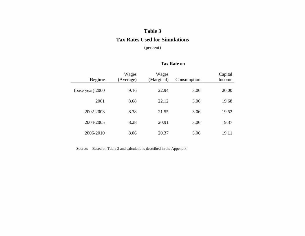
Table 3Tax Rates Used for Simulations

(percent)

Tax Rate on

RegimeWages

(Average)Wages

(Marginal) ConsumptionCapitalIncome

(base year) 2000 9.16 22.94 3.06 20.00

2001 8.68 22.12 3.06 19.68

2002-2003 8.38 21.55 3.06 19.52

2004-2005 8.28 20.91 3.06 19.37

2006-2010 8.06 20.37 3.06 19.11

Source: Based on Table 2 and calculations described in the Appendix

Figure 1 National Saving Rate

0.027

0.031

0.035

0.039

0.043

0.047

0.051

0.055

2000 2002 2004 2006 2008 2010 2012 2014 2016 2018 2020 2150

Year

Savi

ng R

ate w10

k10w15k15k20

Figure 2Capital Stock Relative to Baseline

0.88

0.90

0.92

0.94

0.96

0.98

1.00

1.02

2001 2006 2011 2016 2021 2026 2031 2036 2041 2046 2150

Year

Rat

io

w10k10w15k15k20

Figure 3Output Relative to Baseline

0.975

0.980

0.985

0.990

0.995

1.000

1.005

1.010

1.015

1.020

2000 2002 2004 2006 2008 2010 2012 2014 2016 2018 2020 2150

Year

Rat

io

w10k10w15k15k20

Figure 4Recoupment of Static Revenue Loss

0.00

0.05

0.10

0.15

0.20

0.25

0.30

0.35

0.40

0.45

0.50

2001 2002 2003 2004 2005 2006 2007 2008 2009 2010

Year

Frac

tion

Rec

oupe

d

w10k10w15k15k20

Figure 5Full Dynamic Effect

0.00

0.05

0.10

0.15

0.20

0.25

0.30

0.35

0.40

0.45

0.50

2001 2002 2003 2004 2005 2006 2007 2008 2009 2010

Year

Frac

tion

Rec

oupe

d

w10k10w15k15k20

Figure 6Sensitivity Analysis: Saving Rate

0.027

0.031

0.035

0.039

0.043

0.047

0.051

0.055

2000 2002 2004 2006 2008 2010 2012 2014 2016 2018 2020 2150

Year

Savi

ng R

ate

k10k10r3k10g1

Figure 7Government Spending Response: Saving Rate (10 Year Cut)

0.027

0.031

0.035

0.039

0.043

0.047

0.051

0.055

2000 2002 2004 2006 2008 2010 2012 2014 2016 2018 2020 2150

Year

Savi

ng R

ate

k10k10cak10ch

Figure 8Government Spending Response: Saving Rate (20 Year Cut)

0.027

0.031

0.035

0.039

0.043

0.047

0.051

0.055

2000 2002 2004 2006 2008 2010 2012 2014 2016 2018 2020 2150

Year

Savi

ng R

ate

k20k20cak20ch

Figure 9Open Economy: Saving Rate

0.027

0.031

0.035

0.039

0.043

0.047

0.051

0.055

2000 2002 2004 2006 2008 2010 2012 2014 2016 2018 2020 2150

Year

Savi

ng R

ate

k10k10oe

Figure 10Low Interest Rate: Saving Rate

0.027

0.031

0.035

0.039

0.043

0.047

0.051

0.055

2000 2002 2004 2006 2008 2010 2012 2014 2016 2018 2020 2150

Year

Savi

ng R

ate w10

k10w10sk10s