The Box-Cox Transformation and ARIMA Model Fitting §4.3: Variance Stabilizing Transformations §6.1: ARIMA Model Identification Homework 3b Mathematical Formulation Suppose the variance of a time series Z t satisfies var(Z t )= cf (μ t ) We wish to find a transformation such that,T (·), such that var[T (Z t )] is constant. A first-order Taylor series of T (Z t ) about μ t is T (Z t ) ≈ T (μ t )+ T 0 (μ t )(Z t - μ t ) Now var[T (Z t )] is approximated as var [T (Z t )] ≈ T 0 (μ t ) 2 var(Z t )= c T 0 (μ t ) 2 f (μ t ) Therefore T (·) is chosen such that T 0 (μ t )= 1 p f (μ t ) which implies T (μ t )= Z 1 p f (μ ) dmu t Arthur Berg The Box-Cox Transformation and ARIMA Model Fitting 3/ 18 §4.3: Variance Stabilizing Transformations §6.1: ARIMA Model Identification Homework 3b Box-Cox Transformation Transforming the time series can suppress large fluctuations. The most standard transformation is the log transformation where the new series y t is given by y t = log x t An alternative to the log transformation is the Box-Cox transformation: y t = ( (x λ t - 1)/λ, λ 6= 0 ln x t , λ = 0 Many other transformations are suggested here. Arthur Berg The Box-Cox Transformation and ARIMA Model Fitting 4/ 18 §4.3: Variance Stabilizing Transformations §6.1: ARIMA Model Identification Homework 3b Box-Cox in R > library(MASS) > library(forecast) > x<-rnorm(100)^2 > ts.plot(x) > truehist(x) Arthur Berg The Box-Cox Transformation and ARIMA Model Fitting 5/ 18

Welcome message from author
This document is posted to help you gain knowledge. Please leave a comment to let me know what you think about it! Share it to your friends and learn new things together.
Transcript
The Box-Cox Transformation and ARIMA Model Fitting§4.3: Variance Stabilizing Transformations §6.1: ARIMA Model Identification Homework 3b
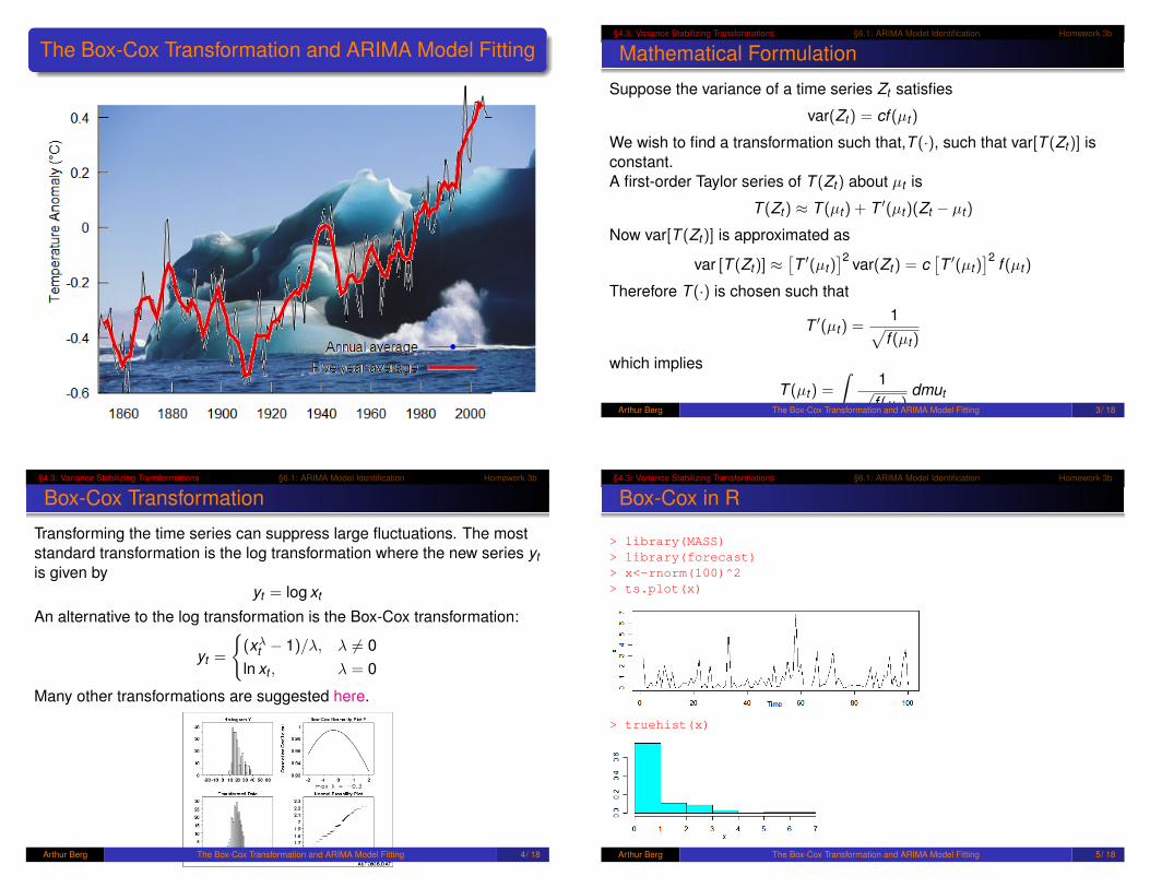
Mathematical Formulation
Suppose the variance of a time series Zt satisfies
var(Zt) = cf (µt)
We wish to find a transformation such that,T (·), such that var[T (Zt)] isconstant.A first-order Taylor series of T (Zt) about µt is
T (Zt) ≈ T (µt) + T ′(µt)(Zt − µt)
Now var[T (Zt)] is approximated as
var [T (Zt)] ≈[T ′(µt)
]2 var(Zt) = c[T ′(µt)
]2 f (µt)
Therefore T (·) is chosen such that
T ′(µt) =1√f (µt)
which implies
T (µt) =
∫1√f (µt)
dmutArthur Berg The Box-Cox Transformation and ARIMA Model Fitting 3/ 18
§4.3: Variance Stabilizing Transformations §6.1: ARIMA Model Identification Homework 3b
Box-Cox Transformation
Transforming the time series can suppress large fluctuations. The moststandard transformation is the log transformation where the new series ytis given by
yt = log xt
An alternative to the log transformation is the Box-Cox transformation:
yt =
{(xλ
t − 1)/λ, λ 6= 0ln xt , λ = 0
Many other transformations are suggested here.
Arthur Berg The Box-Cox Transformation and ARIMA Model Fitting 4/ 18
§4.3: Variance Stabilizing Transformations §6.1: ARIMA Model Identification Homework 3b
Box-Cox in R
> library(MASS)> library(forecast)> x<-rnorm(100)^2> ts.plot(x)
> truehist(x)
Arthur Berg The Box-Cox Transformation and ARIMA Model Fitting 5/ 18

§4.3: Variance Stabilizing Transformations §6.1: ARIMA Model Identification Homework 3b
Box-Cox in R (II)
> bc<-boxcox(x~1)> lam<-bc$x[which.max(bc$y)]> lam
[1] 0.2222222
> truehist(BoxCox(x,lam))
> ts.plot(BoxCox(x,lam))
Arthur Berg The Box-Cox Transformation and ARIMA Model Fitting 6/ 18
§4.3: Variance Stabilizing Transformations §6.1: ARIMA Model Identification Homework 3b
Some Very Old Data
Arthur Berg The Box-Cox Transformation and ARIMA Model Fitting 8/ 18
§4.3: Variance Stabilizing Transformations §6.1: ARIMA Model Identification Homework 3b
Glacial Varves
variation in thickness ∝ amount deposited
Arthur Berg The Box-Cox Transformation and ARIMA Model Fitting 9/ 18
§4.3: Variance Stabilizing Transformations §6.1: ARIMA Model Identification Homework 3b
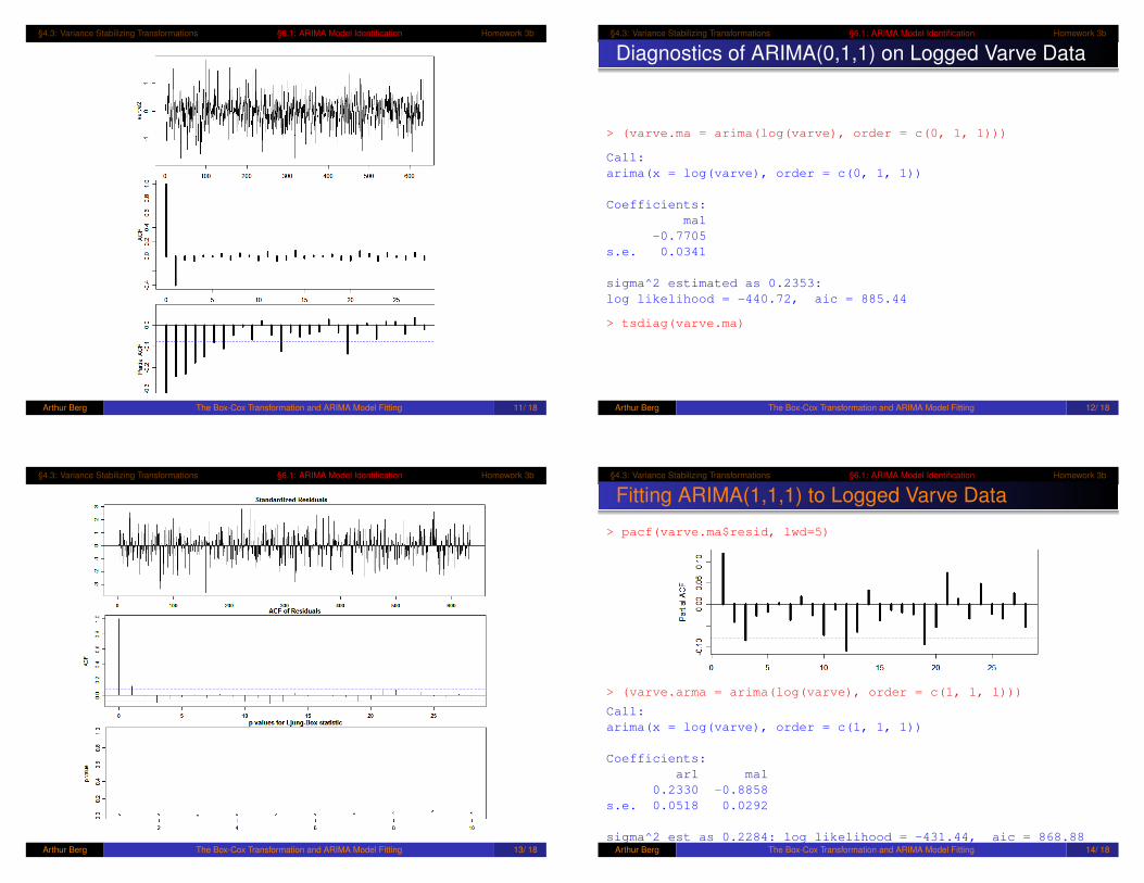
Transformed Glacial Varve Series
The transformation ∇ log(varve) appears appropriate althoughfractional differencing may be in order.Let’s take a closer look at ∇ log(varve).> varve = scan("mydata/varve.dat")> varve2=diff(log(varve))> ts.plot(varve2)> acf(varve2,lwd=5)> pacf(varve2,lwd=5)
Arthur Berg The Box-Cox Transformation and ARIMA Model Fitting 10/ 18
§4.3: Variance Stabilizing Transformations §6.1: ARIMA Model Identification Homework 3b
Arthur Berg The Box-Cox Transformation and ARIMA Model Fitting 11/ 18
§4.3: Variance Stabilizing Transformations §6.1: ARIMA Model Identification Homework 3b
Diagnostics of ARIMA(0,1,1) on Logged Varve Data
> (varve.ma = arima(log(varve), order = c(0, 1, 1)))
Call:arima(x = log(varve), order = c(0, 1, 1))
Coefficients:ma1
-0.7705s.e. 0.0341
sigma^2 estimated as 0.2353:log likelihood = -440.72, aic = 885.44
> tsdiag(varve.ma)
Arthur Berg The Box-Cox Transformation and ARIMA Model Fitting 12/ 18
§4.3: Variance Stabilizing Transformations §6.1: ARIMA Model Identification Homework 3b
Arthur Berg The Box-Cox Transformation and ARIMA Model Fitting 13/ 18
§4.3: Variance Stabilizing Transformations §6.1: ARIMA Model Identification Homework 3b
Fitting ARIMA(1,1,1) to Logged Varve Data
> pacf(varve.ma$resid, lwd=5)
> (varve.arma = arima(log(varve), order = c(1, 1, 1)))
Call:arima(x = log(varve), order = c(1, 1, 1))
Coefficients:ar1 ma1
0.2330 -0.8858s.e. 0.0518 0.0292
sigma^2 est as 0.2284: log likelihood = -431.44, aic = 868.88Arthur Berg The Box-Cox Transformation and ARIMA Model Fitting 14/ 18
§4.3: Variance Stabilizing Transformations §6.1: ARIMA Model Identification Homework 3b
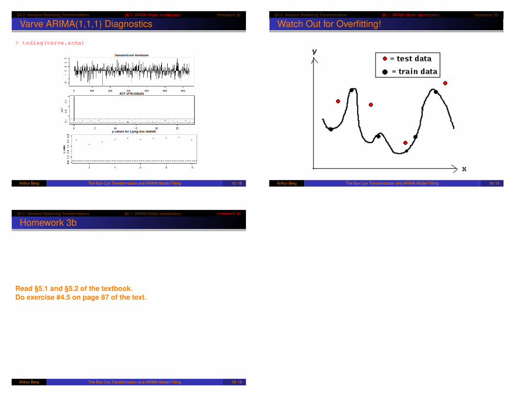
Varve ARIMA(1,1,1) Diagnostics
> tsdiag(varve.arma)
Arthur Berg The Box-Cox Transformation and ARIMA Model Fitting 15/ 18
§4.3: Variance Stabilizing Transformations §6.1: ARIMA Model Identification Homework 3b
Watch Out for Overfitting!
Arthur Berg The Box-Cox Transformation and ARIMA Model Fitting 16/ 18
§4.3: Variance Stabilizing Transformations §6.1: ARIMA Model Identification Homework 3b
Homework 3b
Read §5.1 and §5.2 of the textbook.Do exercise #4.5 on page 87 of the text.
Arthur Berg The Box-Cox Transformation and ARIMA Model Fitting 18/ 18
Related Documents