The BNB Quarterly Projection Model Emilia Penkova and Svilen Pachedzhiev.

The BNB Quarterly Projection Model

Emilia Penkova and Svilen Pachedzhiev

The BNB Quarterly Projection Model

Twinning Project “Adjustment of the Bulgarian National Bank to operate as a full-fledged member of the European System of Central Banks and the Euro-system”

Component 2: Research and preparation for monetary policy operations in line with ECB best practices

Introduction The first version of the Bulgarian National Bank Quarterly

Projection Model (BNBQM) which belongs to the group of traditional structural macroeconomic models.

The model is similar to the European System of Central Banks multi-country model country blocks. The guiding principle in designing the country blocks is that of close compatibility with the ECB Area-Wide Model.

The development of a model over the period 1998-2007 poses formidable challenges, given the short and volatile time series – we calibrate coefficients.

The model is continuously tested and simulated in order to improve it. It should be viewed as work in progress and an area for future empirical research within the BNB, rather than as a finished product.

Introduction

The theoretical background – Neo-Classical Synthesis. The long-run equilibrium is determined by supply side factors (Neo-Classical theory) and short-run fluctuations are demand driven (Keynesian theory).

Backward looking -expectations are reflected via lagged variables, which is considered adequate for the purpose of generating short- to medium-term forecasts.

Behavioral equations – error correction form (Engle Granger two step procedure has been employed).

The purpose of the BNBQM is twofold:

First, to produce macroeconomic forecasts for the Bulgarian economy.

Second, to assess the effects of economic shocks on the Bulgarian economy in simulated scenario analyses.

Outline of Presentation

Theoretical background

Structure of the model and estimated equations

Simulations

Concluding remarks and extensions of research

Supply side of the Economy

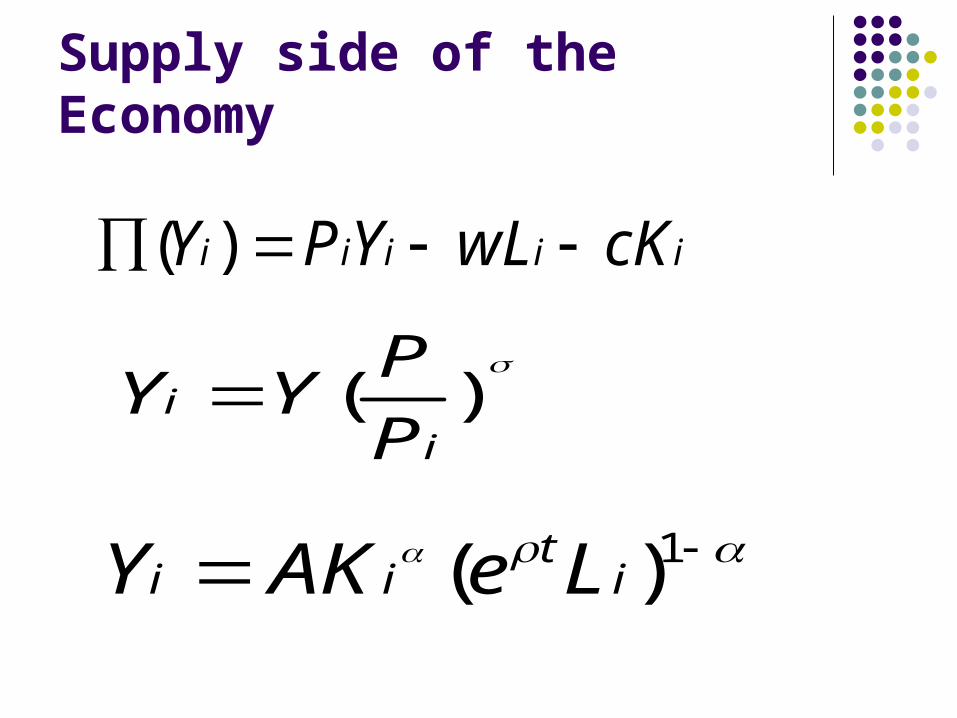
The standard theory of monopolistic competition is applied.

Profits of an individual firm are determined by returns from sale with costs of labour and capital subtracted.

The production process is represented by a Cobb Douglas function.

Supply side of the Economy

iiiii cKwLYPY )(

)(i

iP

PYY

1)( it

ii LeAKY

Supply side of the Economy

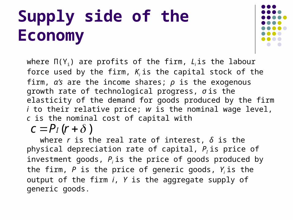
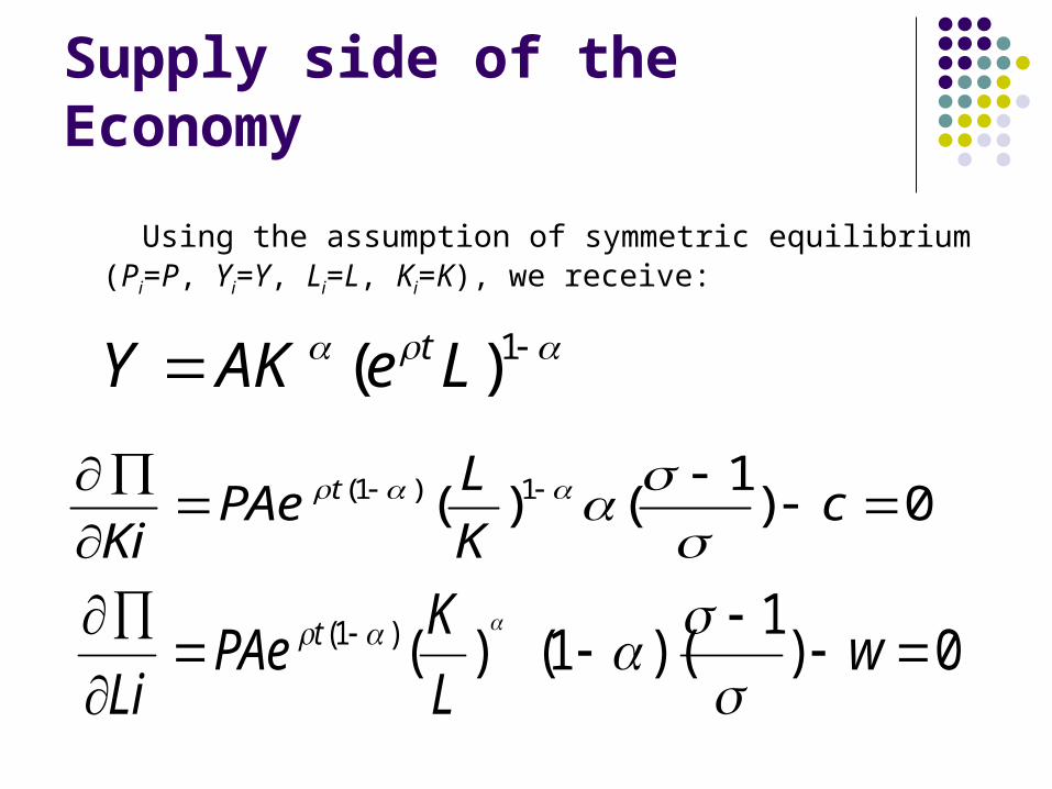
where Π(Yi) are profits of the firm, Li is the labour force used by the firm, Ki is the capital stock of the firm, α’s are the income shares; ρ is the exogenous growth rate of technological progress, σ is the elasticity of the demand for goods produced by the firm i to their relative price; w is the nominal wage level, c is the nominal cost of capital with

where r is the real rate of interest, δ is the physical depreciation rate of capital, PI is price of investment goods, Pi is the price of goods produced by the firm, P is the price of generic goods, Yi is the output of the firm i, Y is the aggregate supply of generic goods.

)( rPc I

Supply side of the Economy

ii

it

iiiii

iiiii

cKwL

LeAKPYcKwLYY

YP

cKwLYPY

1

111

))(()(

)(

Supply side of the Economy

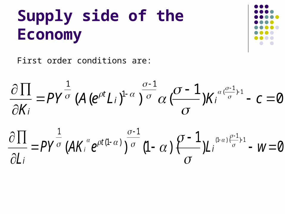
First order conditions are:

0)1

())((1)

1(

11

1

cKLeAPY

Kii

t

i

0)1

)(1()(1)

1)(1(

1)1(

1

wLeAKPY

Li

t

ii

Supply side of the Economy

Using the assumption of symmetric equilibrium (Pi=P, Yi=Y, Li=L, Ki=K), we receive:

1)( LeAKY t

0)1

()( 1)1(

c

K

LPAe

Kit

0)1

)(1()()1(

w

L

KPAe

Lit

Supply side of the Economy

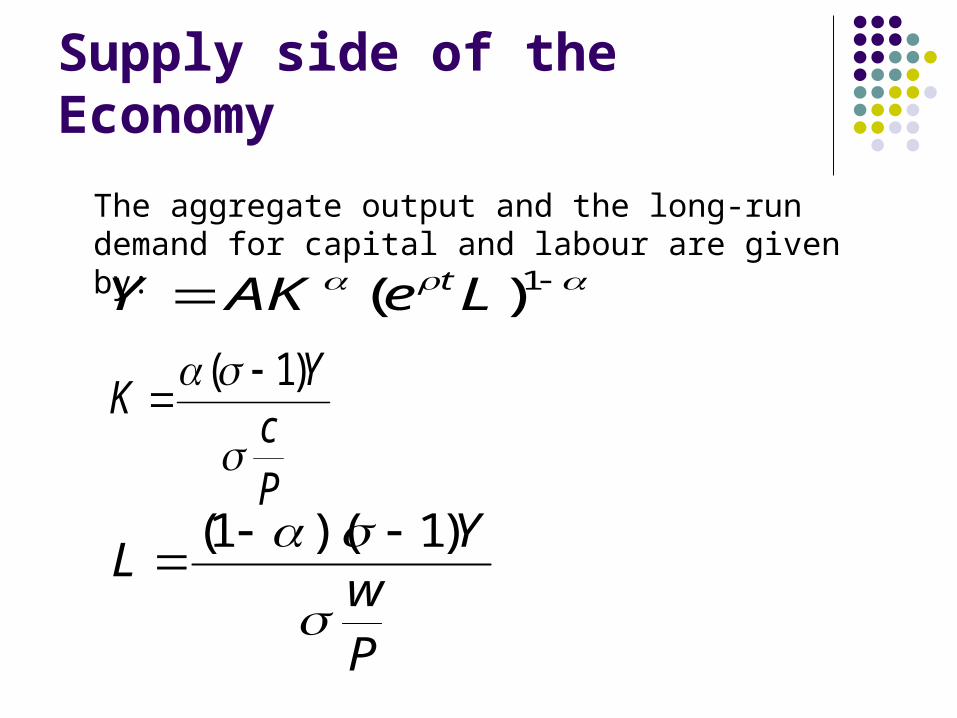
The aggregate output and the long-run demand for capital and labour are given by:

1)( LeAKY t

PcY

K

)1(

Pw

YL

)1)(1(

Structure of the model and estimated equations The simulation and projection features of the BNB Quarterly

Projection Model are driven by twenty behavioural equations and additional forty three identities. Around one hundred and sixty variables enter the model.

The model is in Eviews 5.1 (a program file which imports the data, estimates equations, solves the model and produces forecasts output).

The model is structured into five blocks: production function and factor demand equations, aggregate demand, prices and wages, monetary, and fiscal sector.

Model linkages

Labour market

External sector

Rest of the world Domestic demand

Monetary sector

Fiscal sector

Wages Prices

Error correction form

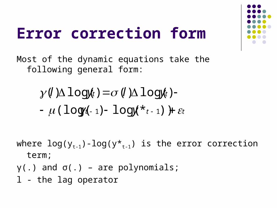
Most of the dynamic equations take the following general form:

where log(yt-1)-log(y*t-1) is the error correction term;

γ(.) and σ(.) – are polynomials;

l - the lag operator

ttt

tt

yy

ylyl

))*log()(log(

)log()()log()(

11

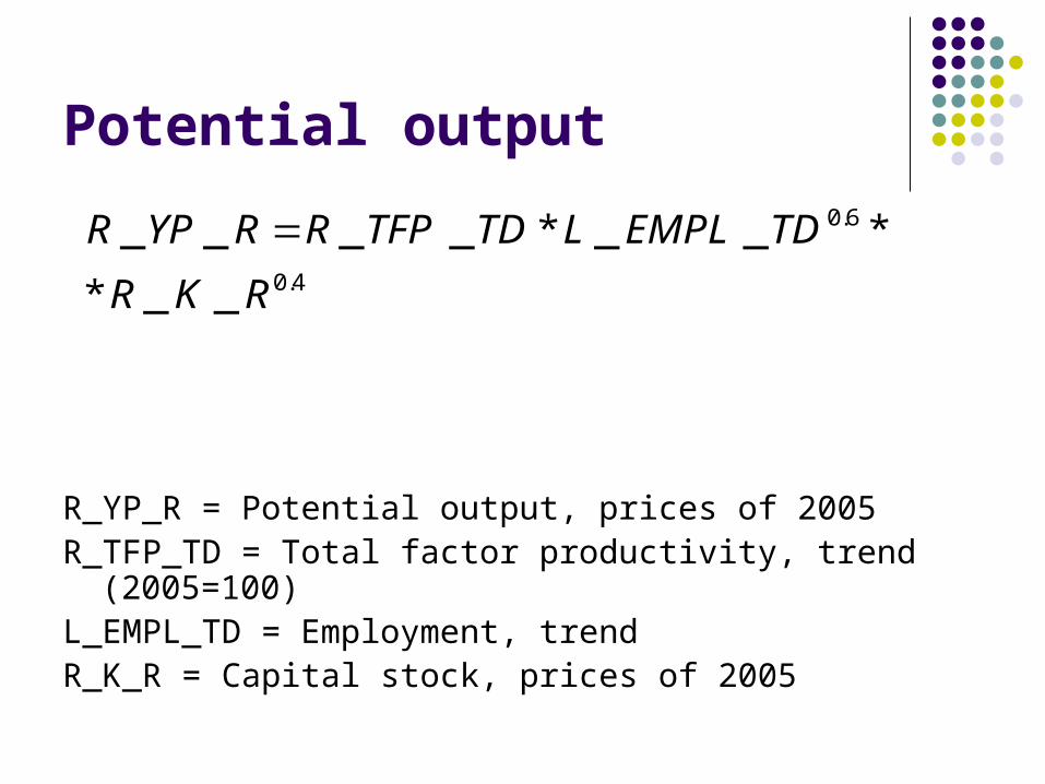
Potential output

R_YP_R = Potential output, prices of 2005R_TFP_TD = Total factor productivity, trend (2005=100)L_EMPL_TD = Employment, trendR_K_R = Capital stock, prices of 2005

4.0

6.0

__*

*__*____

RKR

TDEMPLLTDTFPRRYPR

Potential output

Total factor productivity is estimated as a residual from the production function for the estimated period then using Hodrick-Prescott filter we receive the trend.

The potential employment is received from a labour force forecast and estimated NAIRU.

NAIRU is assumed to be at around 7.7% level (slightly decreasing over the forecasting period) and is estimated using Elmeskov (1993) approach.

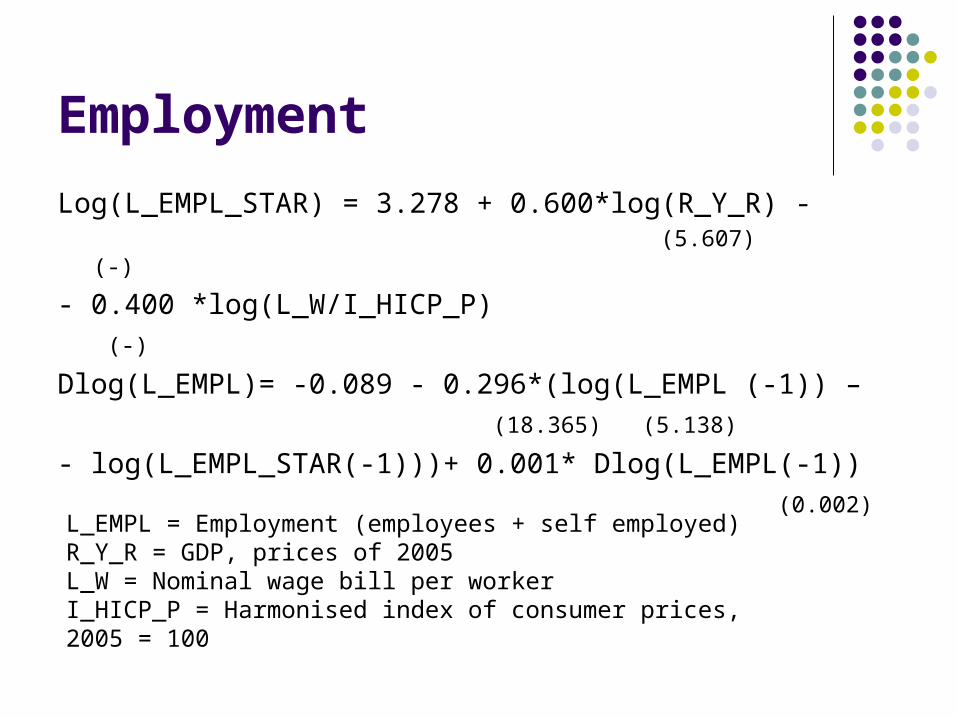
Employment

Log(L_EMPL_STAR) = 3.278 + 0.600*log(R_Y_R) - (5.607) (-)

- 0.400 *log(L_W/I_HICP_P)

(-)

Dlog(L_EMPL)= -0.089 - 0.296*(log(L_EMPL (-1)) –

(18.365) (5.138)

- log(L_EMPL_STAR(-1)))+ 0.001* Dlog(L_EMPL(-1))

(0.002)

L_EMPL = Employment (employees + self employed)R_Y_R = GDP, prices of 2005L_W = Nominal wage bill per workerI_HICP_P = Harmonised index of consumer prices, 2005 = 100

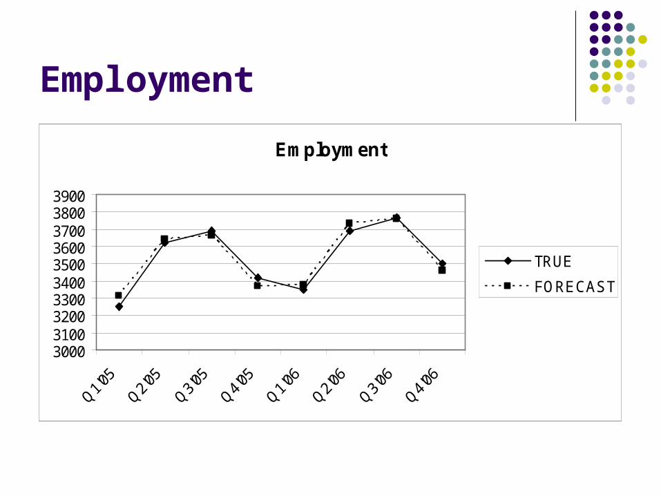
Employment

Employment

3000310032003300340035003600370038003900

TRUE

FORECAST

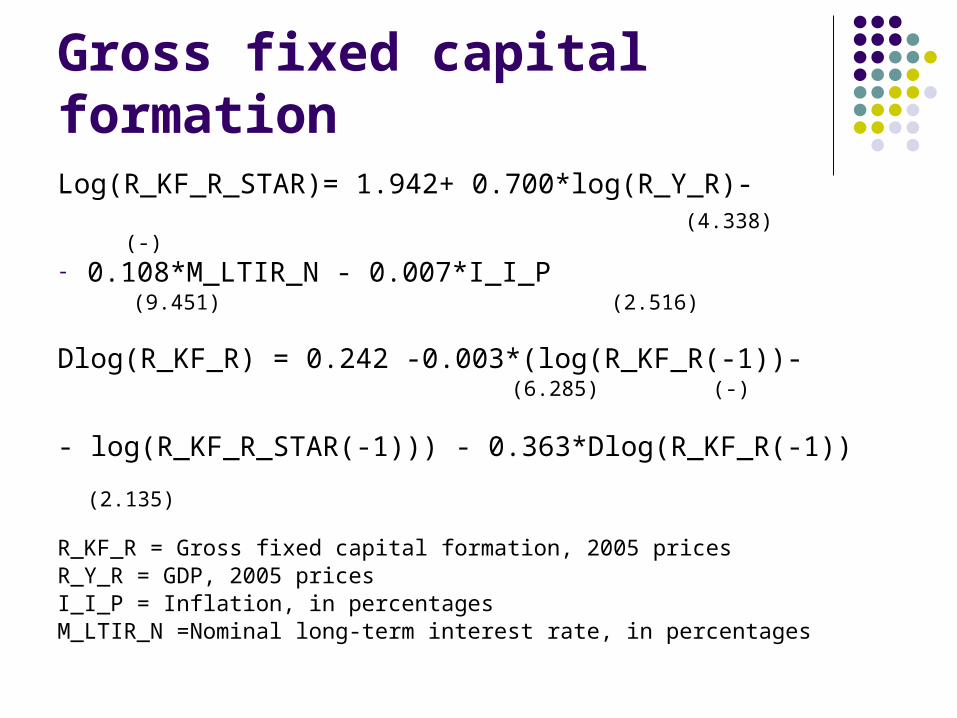
Gross fixed capital formationLog(R_KF_R_STAR)= 1.942+ 0.700*log(R_Y_R)- (4.338) (-)- 0.108*M_LTIR_N - 0.007*I_I_P (9.451) (2.516)

Dlog(R_KF_R) = 0.242 -0.003*(log(R_KF_R(-1))- (6.285) (-)

- log(R_KF_R_STAR(-1))) - 0.363*Dlog(R_KF_R(-1)) (2.135)

R_KF_R = Gross fixed capital formation, 2005 pricesR_Y_R = GDP, 2005 pricesI_I_P = Inflation, in percentagesM_LTIR_N =Nominal long-term interest rate, in percentages

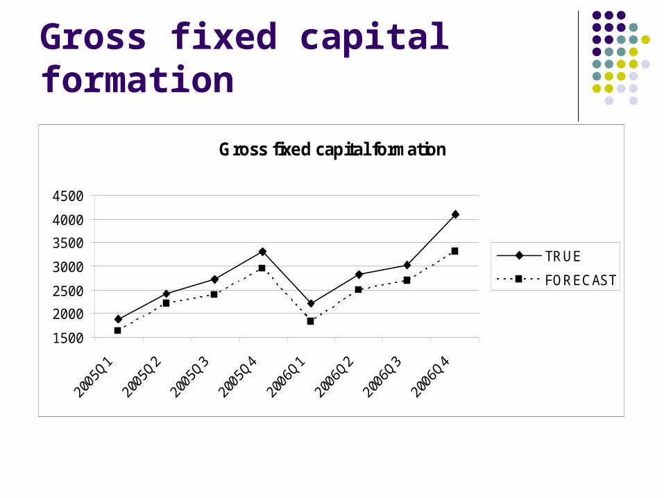
Gross fixed capital formation

Gross fixed capital formation

1500

2000

2500

3000

3500

4000

4500

TRUE

FORECAST

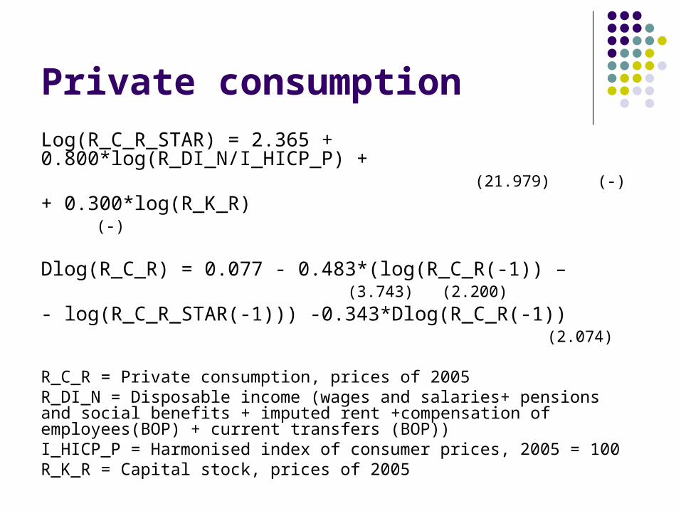
Private consumption

Log(R_C_R_STAR) = 2.365 + 0.800*log(R_DI_N/I_HICP_P) + (21.979) (-)

+ 0.300*log(R_K_R) (-)

Dlog(R_C_R) = 0.077 - 0.483*(log(R_C_R(-1)) – (3.743) (2.200)

- log(R_C_R_STAR(-1))) -0.343*Dlog(R_C_R(-1)) (2.074)

R_C_R = Private consumption, prices of 2005 R_DI_N = Disposable income (wages and salaries+ pensions and social benefits + imputed rent +compensation of employees(BOP) + current transfers (BOP)) I_HICP_P = Harmonised index of consumer prices, 2005 = 100R_K_R = Capital stock, prices of 2005

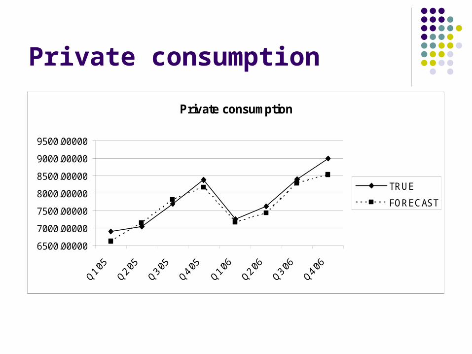
Private consumption

Private consumption

6500.00000

7000.00000

7500.00000

8000.00000

8500.00000

9000.00000

9500.00000

TRUE

FORECAST

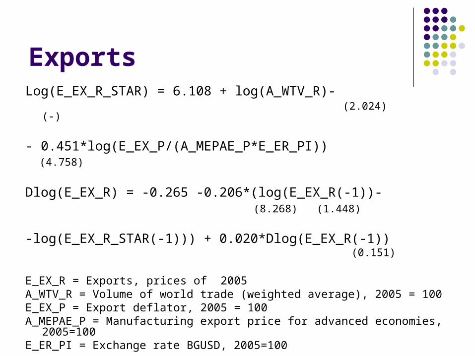
ExportsLog(E_EX_R_STAR) = 6.108 + log(A_WTV_R)- (2.024) (-)

- 0.451*log(E_EX_P/(A_MEPAE_P*E_ER_PI)) (4.758)

Dlog(E_EX_R) = -0.265 -0.206*(log(E_EX_R(-1))- (8.268) (1.448)

-log(E_EX_R_STAR(-1))) + 0.020*Dlog(E_EX_R(-1)) (0.151)

E_EX_R = Exports, prices of 2005 A_WTV_R = Volume of world trade (weighted average), 2005 = 100E_EX_P = Export deflator, 2005 = 100A_MEPAE_P = Manufacturing export price for advanced economies, 2005=100E_ER_PI = Exchange rate BGUSD, 2005=100

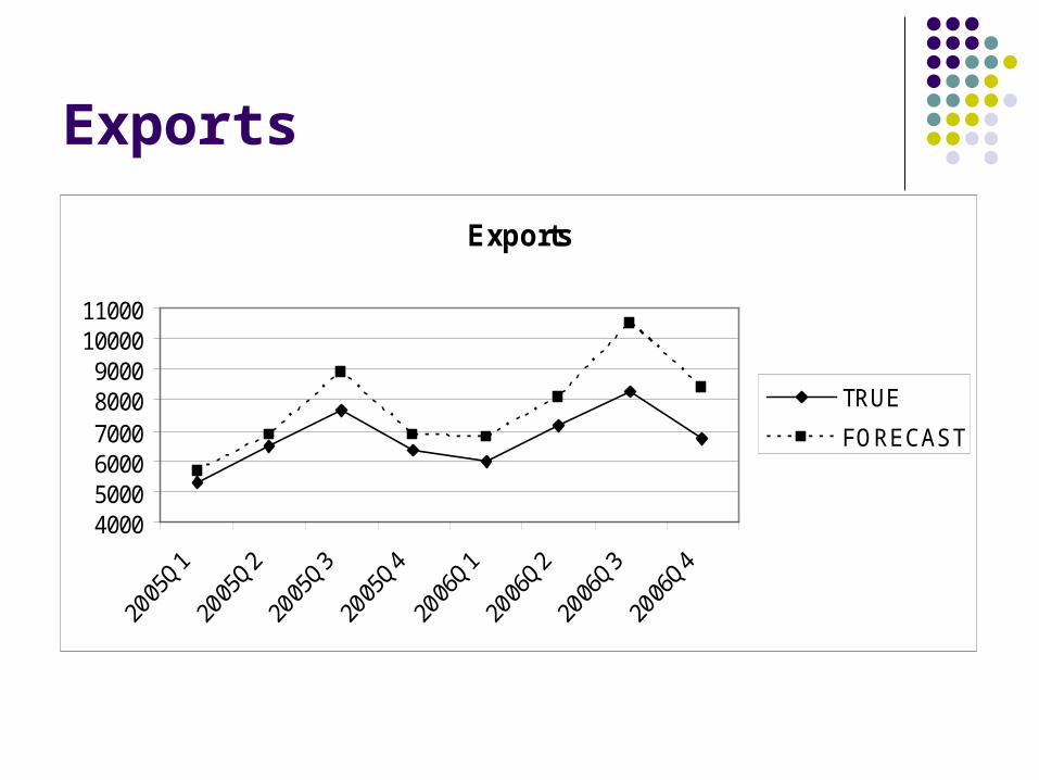
Exports

Exports

400050006000700080009000

1000011000

TRUE

FORECAST

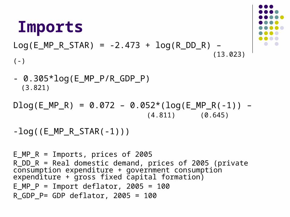
ImportsLog(E_MP_R_STAR) = -2.473 + log(R_DD_R) – (13.023) (-)

- 0.305*log(E_MP_P/R_GDP_P) (3.821)

Dlog(E_MP_R) = 0.072 – 0.052*(log(E_MP_R(-1)) – (4.811) (0.645)

-log((E_MP_R_STAR(-1)))

E_MP_R = Imports, prices of 2005R_DD_R = Real domestic demand, prices of 2005 (private consumption expenditure + government consumption expenditure + gross fixed capital formation)E_MP_P = Import deflator, 2005 = 100 R_GDP_P= GDP deflator, 2005 = 100

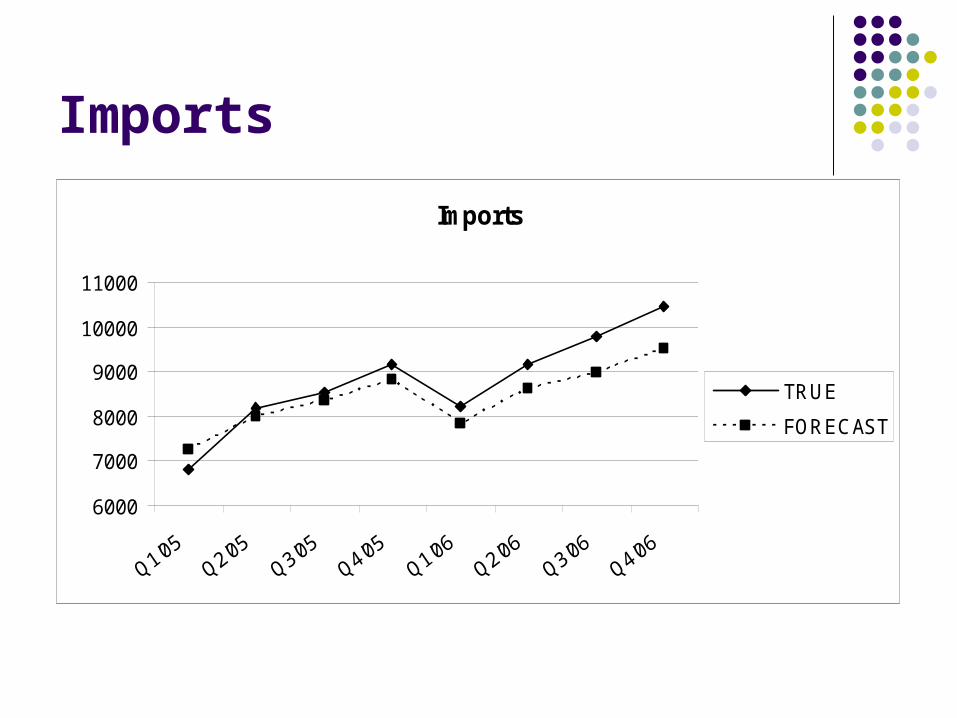
Imports

Imports

6000

7000

8000

9000

10000

11000

TRUE

FORECAST

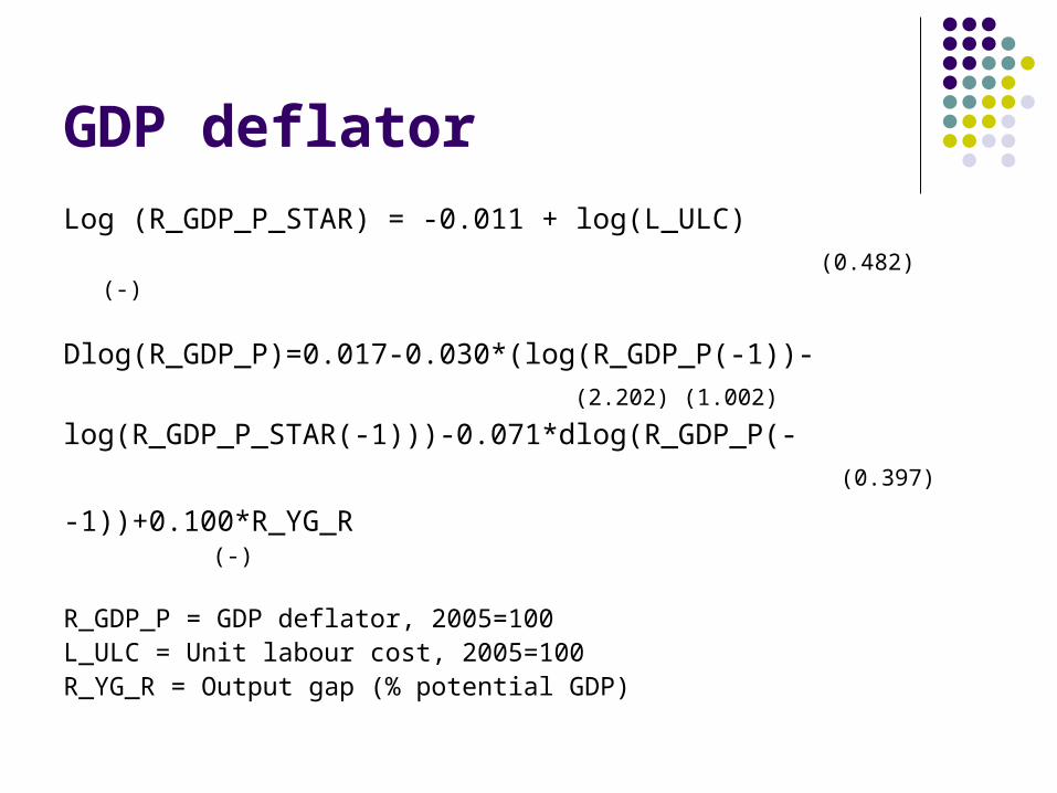
GDP deflator

Log (R_GDP_P_STAR) = -0.011 + log(L_ULC)

(0.482) (-)

Dlog(R_GDP_P)=0.017-0.030*(log(R_GDP_P(-1))-

(2.202) (1.002)

log(R_GDP_P_STAR(-1)))-0.071*dlog(R_GDP_P(-

(0.397)

-1))+0.100*R_YG_R (-)

R_GDP_P = GDP deflator, 2005=100L_ULC = Unit labour cost, 2005=100R_YG_R = Output gap (% potential GDP)

GDP deflator

GDP deflator

0.99

1

1.01

1.02

1.03

1.04

1.05

TRUE

FORECAST

HICP without administered prices

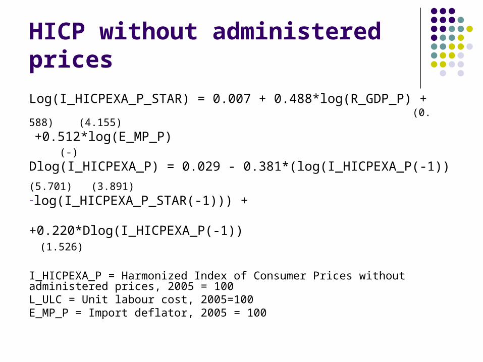
Log(I_HICPEXA_P_STAR) = 0.007 + 0.488*log(R_GDP_P) + (0. 588) (4.155)

+0.512*log(E_MP_P) (-)Dlog(I_HICPEXA_P) = 0.029 - 0.381*(log(I_HICPEXA_P(-1)) (5.701) (3.891) -log(I_HICPEXA_P_STAR(-1))) +

+0.220*Dlog(I_HICPEXA_P(-1))

(1.526) I_HICPEXA_P = Harmonized Index of Consumer Prices without administered prices, 2005 = 100L_ULC = Unit labour cost, 2005=100E_MP_P = Import deflator, 2005 = 100

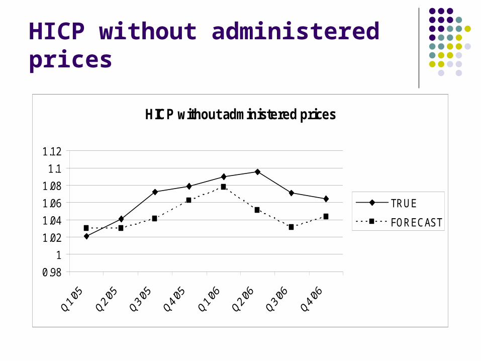
HICP without administered prices

HICP without administered prices

0.98

1

1.02

1.04

1.06

1.08

1.1

1.12

TRUE

FORECAST

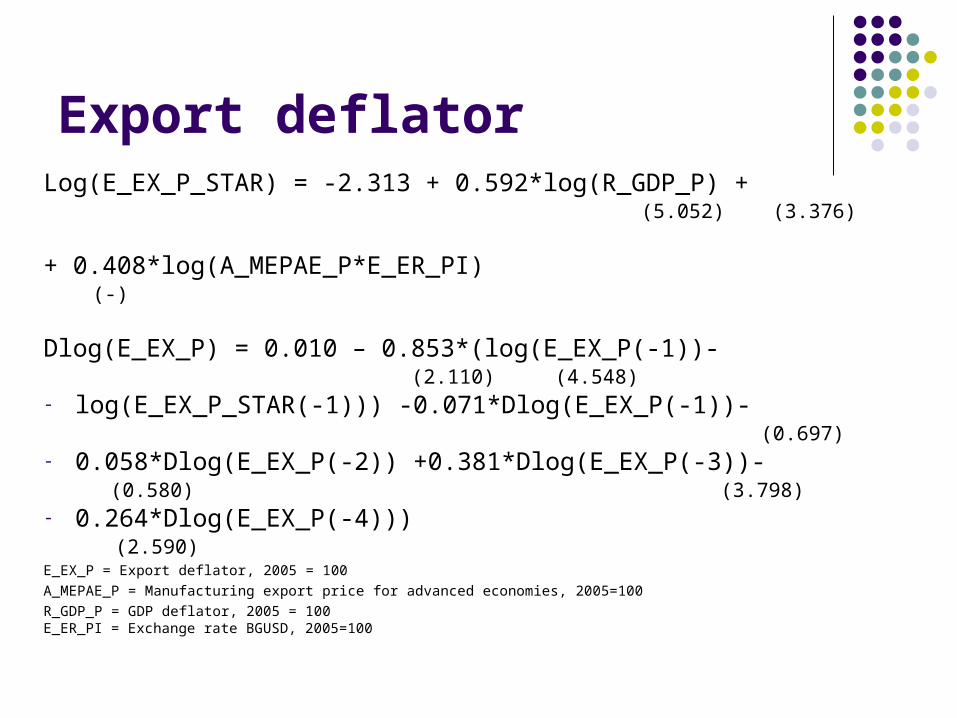
Export deflatorLog(E_EX_P_STAR) = -2.313 + 0.592*log(R_GDP_P) + (5.052) (3.376)

+ 0.408*log(A_MEPAE_P*E_ER_PI) (-)

Dlog(E_EX_P) = 0.010 – 0.853*(log(E_EX_P(-1))- (2.110) (4.548)

- log(E_EX_P_STAR(-1))) -0.071*Dlog(E_EX_P(-1))- (0.697)- 0.058*Dlog(E_EX_P(-2)) +0.381*Dlog(E_EX_P(-3))- (0.580) (3.798)- 0.264*Dlog(E_EX_P(-4))) (2.590)E_EX_P = Export deflator, 2005 = 100

A_MEPAE_P = Manufacturing export price for advanced economies, 2005=100

R_GDP_P = GDP deflator, 2005 = 100E_ER_PI = Exchange rate BGUSD, 2005=100

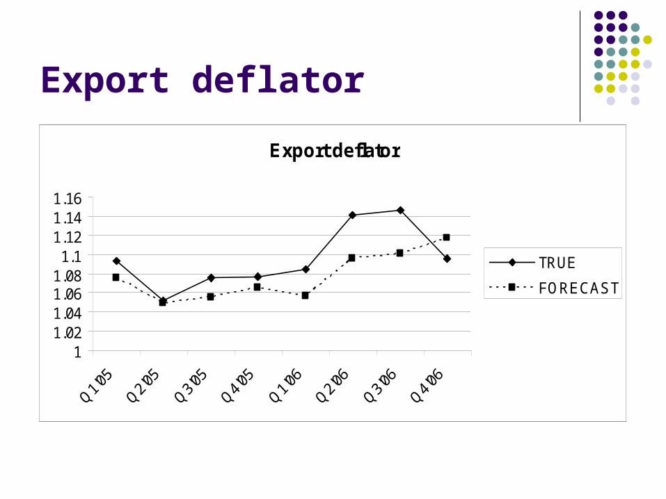
Export deflator

Export deflator

11.021.041.061.081.1

1.121.141.16

TRUE

FORECAST

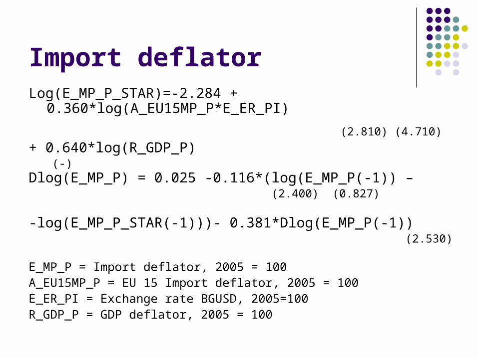
Import deflatorLog(E_MP_P_STAR)=-2.284 + 0.360*log(A_EU15MP_P*E_ER_PI)

(2.810) (4.710)

+ 0.640*log(R_GDP_P) (-)Dlog(E_MP_P) = 0.025 -0.116*(log(E_MP_P(-1)) – (2.400) (0.827)

-log(E_MP_P_STAR(-1)))- 0.381*Dlog(E_MP_P(-1)) (2.530)

E_MP_P = Import deflator, 2005 = 100A_EU15MP_P = EU 15 Import deflator, 2005 = 100E_ER_PI = Exchange rate BGUSD, 2005=100R_GDP_P = GDP deflator, 2005 = 100

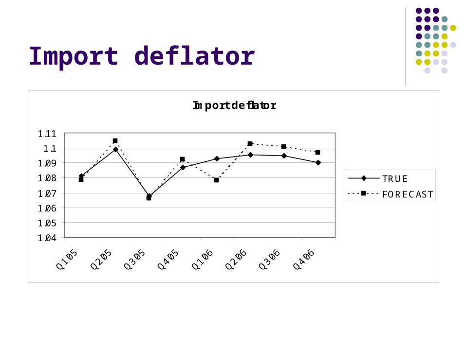
Import deflator

Import deflator

1.04

1.05

1.06

1.07

1.08

1.09

1.1

1.11

TRUE

FORECAST

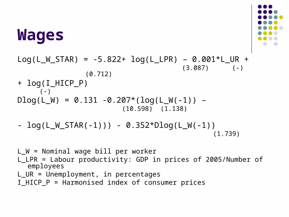
Wages

Log(L_W_STAR) = -5.822+ log(L_LPR) – 0.001*L_UR + (3.087) (-) (0.712)

+ log(I_HICP_P) (-)

Dlog(L_W) = 0.131 -0.207*(log(L_W(-1)) – (10.598) (1.138)

- log(L_W_STAR(-1))) - 0.352*Dlog(L_W(-1)) (1.739)

L_W = Nominal wage bill per workerL_LPR = Labour productivity: GDP in prices of 2005/Number of employees L_UR = Unemployment, in percentagesI_HICP_P = Harmonised index of consumer prices

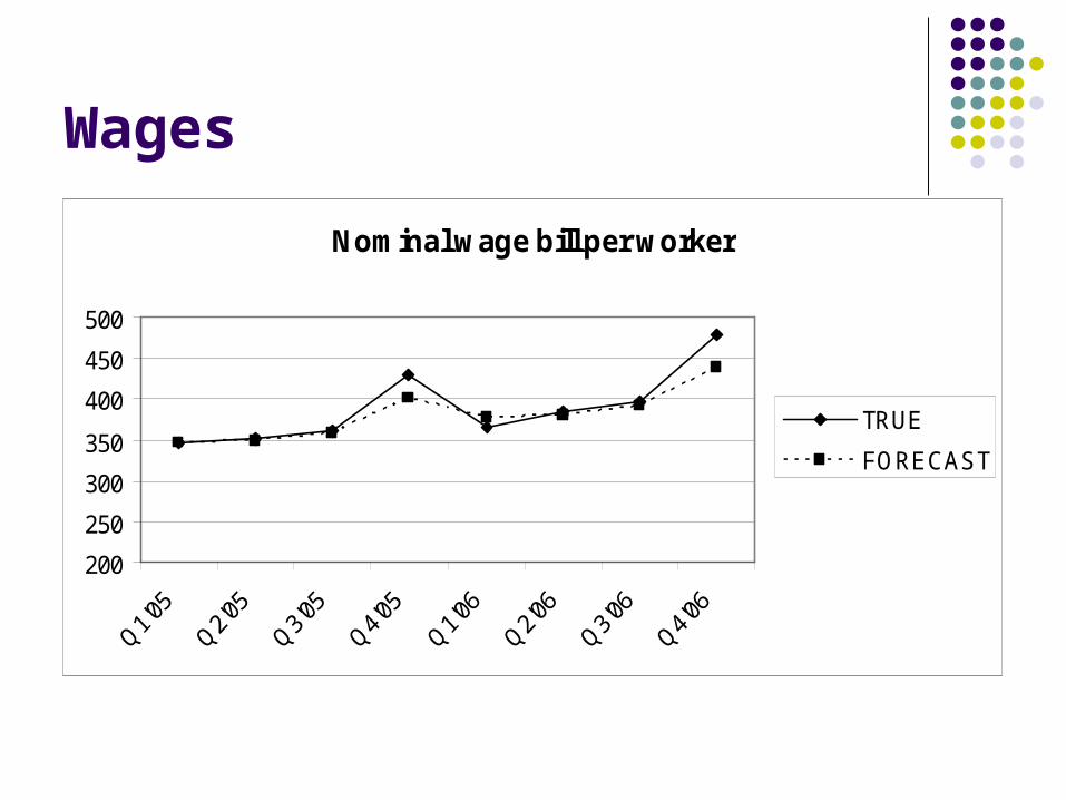
Wages

Nominal wage bill per worker

200

250

300

350

400

450

500

TRUE

FORECAST

Fiscal sector

Government expenditures and government revenues are modelled separately:

The government expenditures are disaggregated into five parts: government consumption, government investment, government transfers, government interest payments and other expenditure.

The government revenues consist of five components: revenues from personal income tax, social security contribution, revenues from corporate income tax, revenues from indirect taxes and other revenue items.

Personal income taxes

G_PIT = G_PIT_TR*R_CE_N

G_PIT = Personal income taxes (million leva)

G_PIT_TR =Personal income effective tax rate

R_CE_N = Compensation of employees (million leva)

Social security contribution

G_SSC=G_SSC_TR*R_CE_N

G_SSC = Social security contribution (incl. employers’ and employees’ contribution in million leva)

G_SSC_TR = Social security effective tax rate

R_CE_N = Compensation of employees (million leva)

Indirect taxes

G_IND=G_IND_TR*R_C_N

G_IND = Indirect taxes (incl. VAT, customs revenue, excise duties)

G_IND_TR = Indirect effective tax rate

R_C_N = Private consumption, in current prices

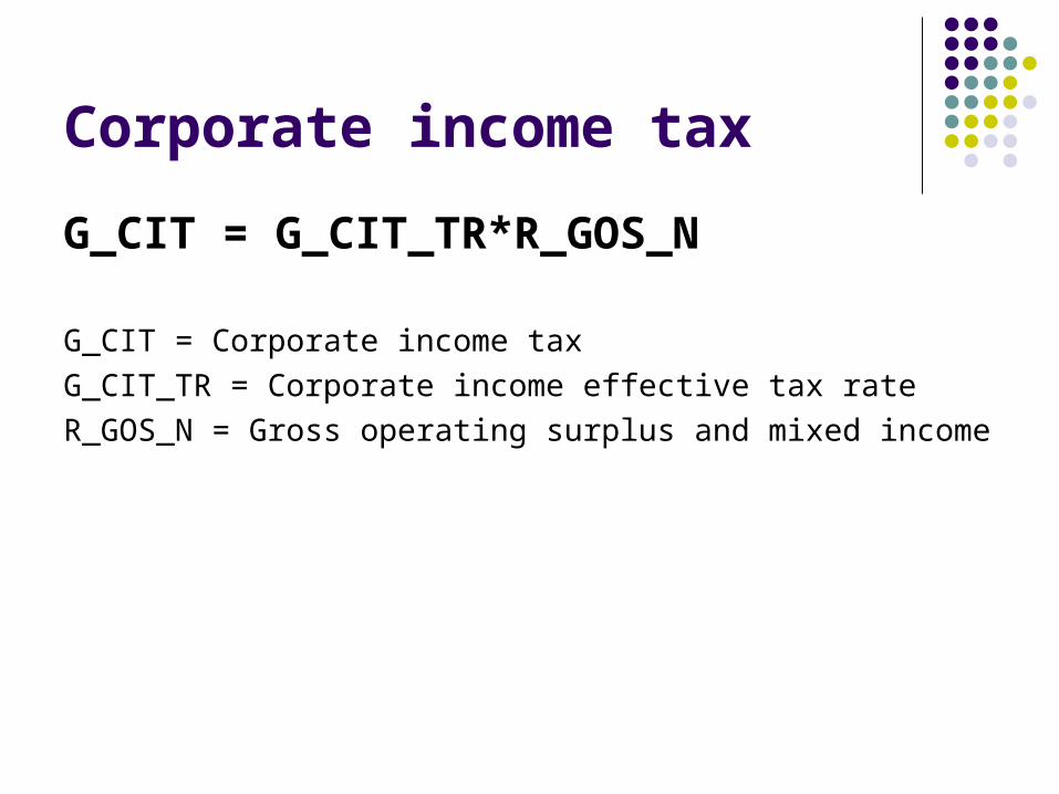
Corporate income tax

G_CIT = G_CIT_TR*R_GOS_N

G_CIT = Corporate income tax

G_CIT_TR = Corporate income effective tax rate

R_GOS_N = Gross operating surplus and mixed income

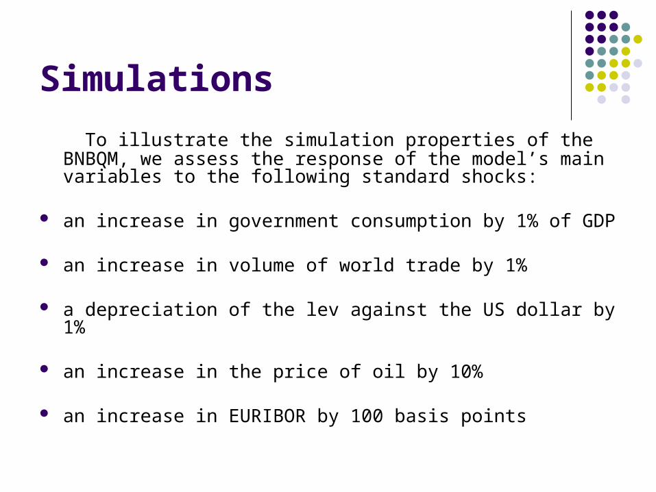
Simulations

To illustrate the simulation properties of the BNBQM, we assess the response of the model’s main variables to the following standard shocks:

an increase in government consumption by 1% of GDP

an increase in volume of world trade by 1%

a depreciation of the lev against the US dollar by 1%

an increase in the price of oil by 10%

an increase in EURIBOR by 100 basis points

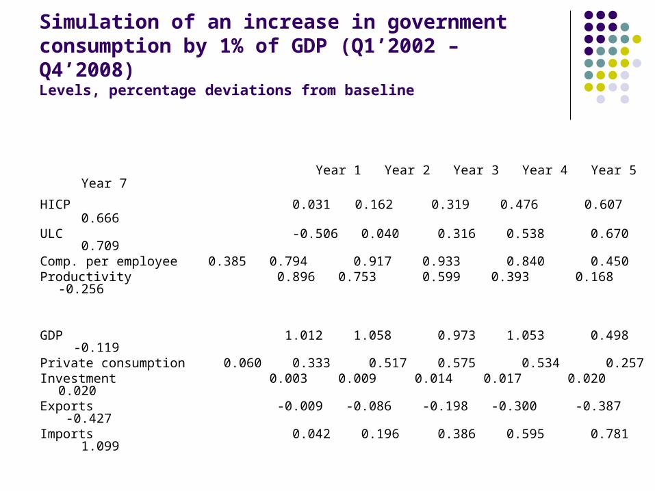
Simulation of an increase in government consumption by 1% of GDP (Q1’2002 – Q4’2008)Levels, percentage deviations from baseline

Year 1 Year 2 Year 3 Year 4 Year 5 Year 7

HICP 0.031 0.162 0.319 0.476 0.607 0.666ULC -0.506 0.040 0.316 0.538 0.670 0.709Comp. per employee 0.385 0.794 0.917 0.933 0.840 0.450Productivity 0.896 0.753 0.599 0.393 0.168 -0.256

GDP 1.012 1.058 0.973 1.053 0.498 -0.119 Private consumption 0.060 0.333 0.517 0.575 0.534 0.257Investment 0.003 0.009 0.014 0.017 0.020 0.020Exports -0.009 -0.086 -0.198 -0.300 -0.387 -0.427Imports 0.042 0.196 0.386 0.595 0.781 1.099

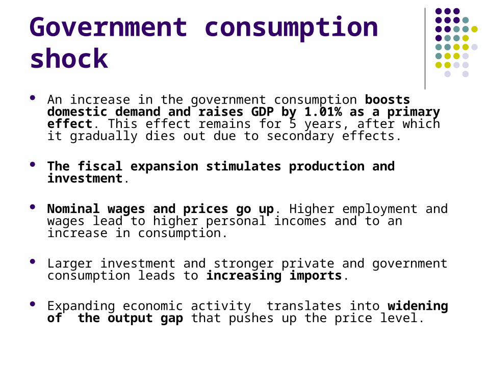
Government consumption shock

An increase in the government consumption boosts domestic demand and raises GDP by 1.01% as a primary effect. This effect remains for 5 years, after which it gradually dies out due to secondary effects.

The fiscal expansion stimulates production and investment.

Nominal wages and prices go up. Higher employment and wages lead to higher personal incomes and to an increase in consumption.

Larger investment and stronger private and government consumption leads to increasing imports.

Expanding economic activity translates into widening of the output gap that pushes up the price level.

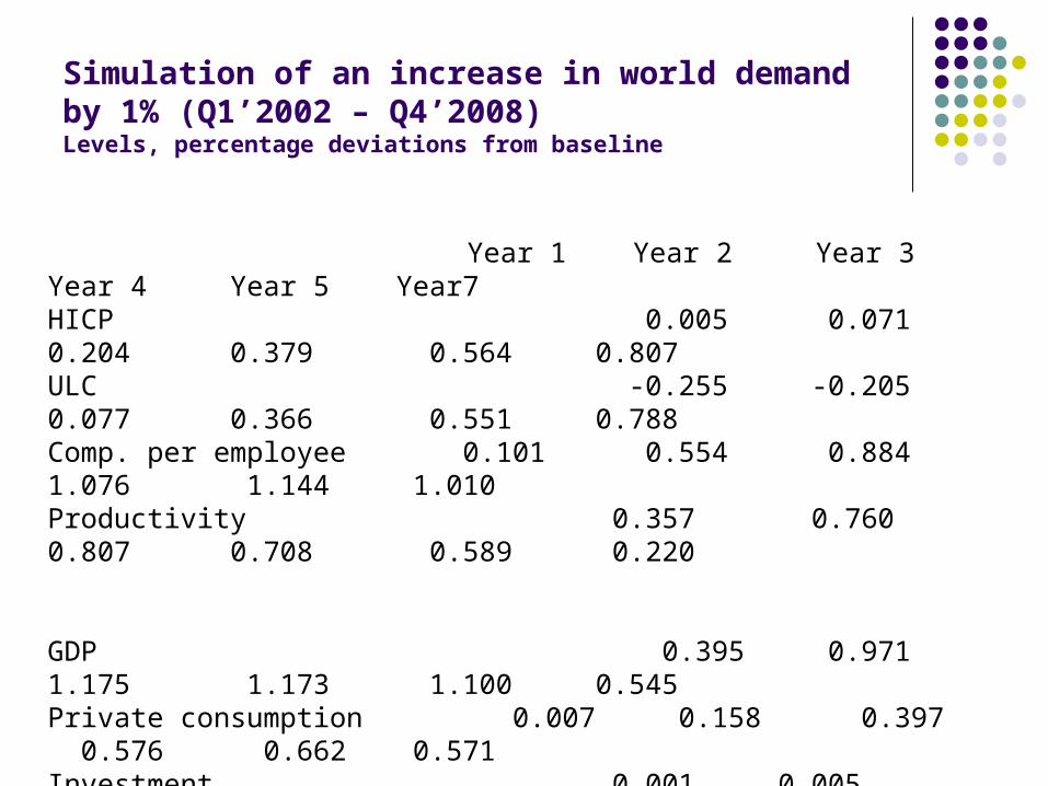
Simulation of an increase in world demand by 1% (Q1’2002 – Q4’2008)Levels, percentage deviations from baseline

Year 1 Year 2 Year 3 Year 4 Year 5 Year7HICP 0.005 0.071 0.204 0.379 0.564 0.807ULC -0.255 -0.205 0.077 0.366 0.551 0.788Comp. per employee 0.101 0.554 0.884 1.076 1.144 1.010Productivity 0.357 0.760 0.807 0.708 0.589 0.220

GDP 0.395 0.971 1.175 1.173 1.100 0.545Private consumption 0.007 0.158 0.397 0.576 0.662 0.571Investment 0.001 0.005 0.011 0.016 0.021 0.027Exports 0.725 1.546 1.583 1.497 1.426 1.320Imports 0.001 0.029 0.106 0.235 0.390 0.728

An increase in world demand This simulation is particularly important because of the openness of

the Bulgarian economy. The external demand shock leads to a stronger domestic demand. The external shock directly drives up the volume of exports by 1.55% (second year), which in turn also increases imports.

Employment and nominal wages increase which leads to higher private consumption (0.57%-seventh year).

Higher aggregate demand widens the output gap that pushes up the aggregate price level.

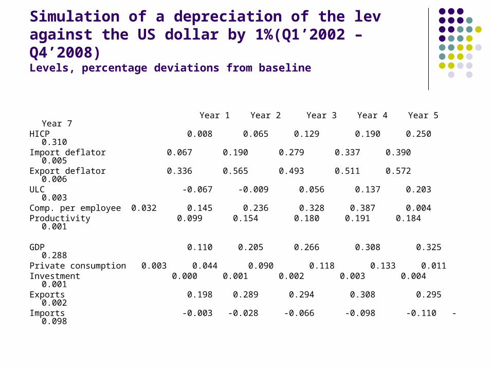
Simulation of a depreciation of the lev against the US dollar by 1%(Q1’2002 – Q4’2008)Levels, percentage deviations from baseline

Year 1 Year 2 Year 3 Year 4 Year 5 Year 7HICP 0.008 0.065 0.129 0.190 0.250 0.310Import deflator 0.067 0.190 0.279 0.337 0.390 0.005Export deflator 0.336 0.565 0.493 0.511 0.572 0.006ULC -0.067 -0.009 0.056 0.137 0.203 0.003Comp. per employee 0.032 0.145 0.236 0.328 0.387 0.004Productivity 0.099 0.154 0.180 0.191 0.184 0.001

GDP 0.110 0.205 0.266 0.308 0.325 0.288Private consumption 0.003 0.044 0.090 0.118 0.133 0.011Investment 0.000 0.001 0.002 0.003 0.004 0.001Exports 0.198 0.289 0.294 0.308 0.295 0.002Imports -0.003 -0.028 -0.066 -0.098 -0.110 -0.098

An exchange rate shock The decrease in the value of the lev against the US dollar has an

immediate impact on both the import and export deflators – they both increase.

HICP increases by 0.25% in the fifth year. Compensation per employee adjusts and income increases which drives the consumption up.

Because of the relative increase in foreign prices, imports decrease and exports increase slightly. The reaction of real GDP to an exchange rate shock achieves its maximum in the fifth year (0.32%).

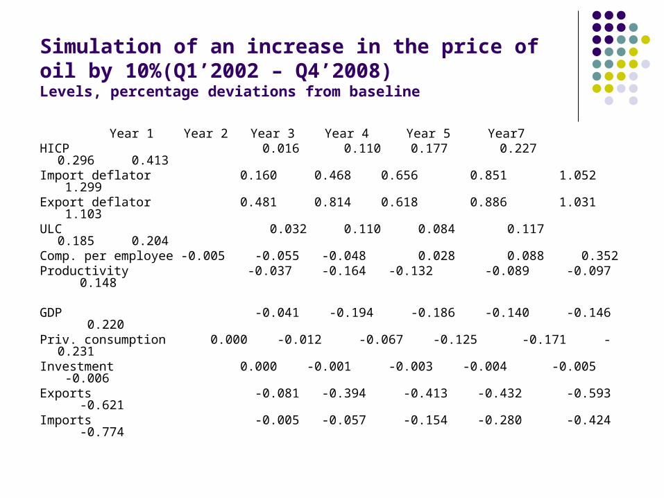
Simulation of an increase in the price of oil by 10%(Q1’2002 – Q4’2008)Levels, percentage deviations from baseline

Year 1 Year 2 Year 3 Year 4 Year 5 Year7

HICP 0.016 0.110 0.177 0.227 0.296 0.413 Import deflator 0.160 0.468 0.656 0.851 1.052 1.299Export deflator 0.481 0.814 0.618 0.886 1.031 1.103ULC 0.032 0.110 0.084 0.117 0.185 0.204Comp. per employee -0.005 -0.055 -0.048 0.028 0.088 0.352Productivity -0.037 -0.164 -0.132 -0.089 -0.097 0.148

GDP -0.041 -0.194 -0.186 -0.140 -0.146 0.220 Priv. consumption 0.000 -0.012 -0.067 -0.125 -0.171 -0.231 Investment 0.000 -0.001 -0.003 -0.004 -0.005 -0.006

Exports -0.081 -0.394 -0.413 -0.432 -0.593 -0.621 Imports -0.005 -0.057 -0.154 -0.280 -0.424 -0.774

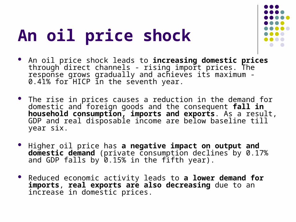
An oil price shock An oil price shock leads to increasing domestic prices through direct

channels - rising import prices. The response grows gradually and achieves its maximum - 0.41% for HICP in the seventh year.

The rise in prices causes a reduction in the demand for domestic and

foreign goods and the consequent fall in household consumption, imports and exports. As a result, GDP and real disposable income are below baseline till year six.

Higher oil price has a negative impact on output and domestic demand (private consumption declines by 0.17% and GDP falls by 0.15% in the fifth year).

Reduced economic activity leads to a lower demand for imports, real exports are also decreasing due to an increase in domestic prices.

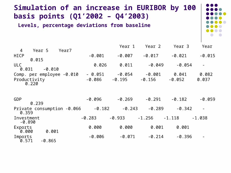
Simulation of an increase in EURIBOR by 100 basis points (Q1’2002 – Q4’2003) Levels, percentage deviations from baseline

Year 1 Year 2 Year 3 Year 4 Year 5 Year7HICP -0.001 -0.007 -0.017 -0.021 -0.015 0.015ULC 0.026 0.011 -0.049 -0.054 -0.031 -0.010Comp. per employee -0.010 - 0.051 -0.054 -0.001 0.041 0.082Productivity -0.086 -0.195 -0.156 -0.052 0.037 0.220

GDP -0.096 -0.269 -0.291 -0.182 -0.059 0.239Private consumption -0.066 -0.182 -0.243 -0.289 -0.342 -0.359Investment -0.283 -0.933 -1.256 -1.118 -1.038 -0.890Exports 0.000 0.000 0.001 0.001 0.000 0.001Imports -0.006 -0.071 -0.214 -0.396 -0.571 -0.865

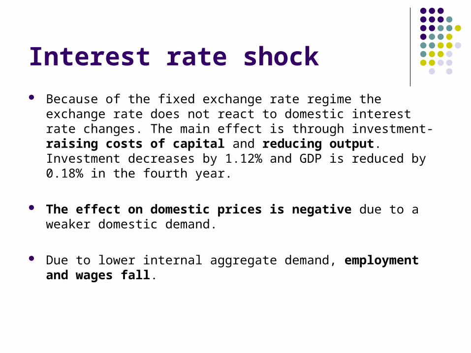
Interest rate shock Because of the fixed exchange rate regime the exchange rate does not

react to domestic interest rate changes. The main effect is through investment- raising costs of capital and reducing output. Investment decreases by 1.12% and GDP is reduced by 0.18% in the fourth year.

The effect on domestic prices is negative due to a weaker domestic demand.

Due to lower internal aggregate demand, employment and wages fall.

Concluding remarks and extensions A first step towards building a structural

macroeconomic model.

This practical work gives valuable information for the future development of the model which needs to be continuously developed and could be improved in a number of respects:

Availability of new data will require re-estimation and re-calibration of the model;

Concluding remarks and extensions

Developing a long-run baseline that reflects a fully theory-consistent long-run steady state;

To consider policy rules in the simulations;

Developing a more detailed representation of the trade block by including services on the one hand and different regions on the other hand;

An extension of forward-looking behaviour. Expectations should be incorporated, particularly to allow for a specific role in price and wage formation.

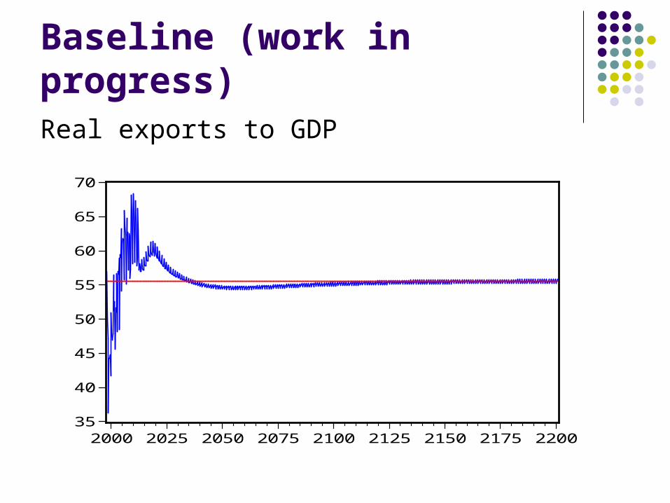
Baseline (work in progress)Real exports to GDP

35

40

45

50

55

60

65

70

2000 2025 2050 2075 2100 2125 2150 2175 2200

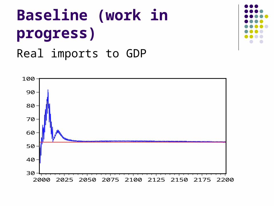
Baseline (work in progress)Real imports to GDP

30

40

50

60

70

80

90

100

2000 2025 2050 2075 2100 2125 2150 2175 2200

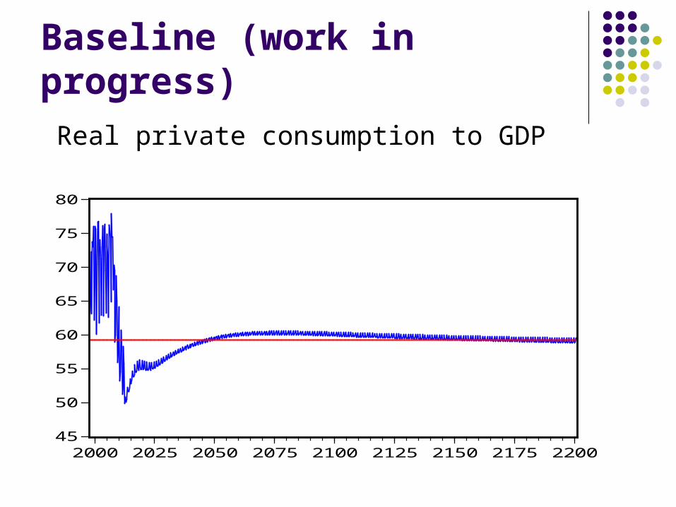
Baseline (work in progress)Real private consumption to GDP

45

50

55

60

65

70

75

80

2000 2025 2050 2075 2100 2125 2150 2175 2200

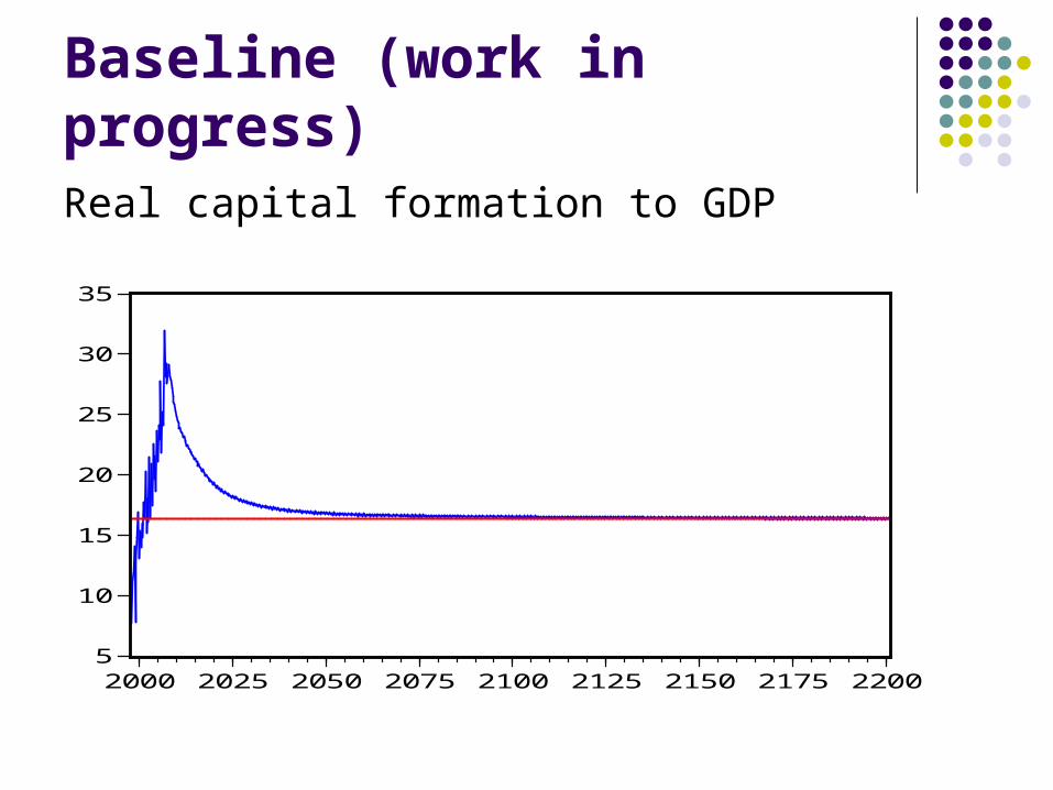
Baseline (work in progress)Real capital formation to GDP

5

10

15

20

25

30

35

2000 2025 2050 2075 2100 2125 2150 2175 2200