The Biobjective TSP with Profit - Middle East Technical ...etd.lib.metu.edu.tr/upload/12608890/index.pdfTHE BIOBJECTIVE TRAVELING SALESMAN PROBLEM WITH ... Kar Getiren GSP, ... Illustration

THE BIOBJECTIVE TRAVELING SALESMAN PROBLEM WITH PROFIT

A THESIS SUBMITTED TO THE GRADUATED SCHOOL OF NATURAL AND APPLIED SCIENCES

OF MIDDLE EAST TECHNCAL UNIVERSITY

BY

ÖMÜR ŞİMŞEK

IN PARTIAL FULFILLMENT OF THE REQUIREMENTS FOR

THE DEGREE OF MASTER OF SCIENCE IN

INDUSTRIAL ENGINEERING

SEPTEMBER 2007

Approval of Thesis:

THE BIOBJECTIVE TRAVELING SALESMAN PROBLEM WITH

PROFITS

submitted by ÖMÜR ŞİMŞEK in partial fulfillment of the requirements for the degree of Master of Science in Industrial Engineering Department, Middle East Technical University by,

Prof. Dr. Canan ÖZGEN Dean, Graduate School of Natural and Applied Sciences

Prof. Dr. Çağlar GÜVEN Head of Department, Industrial Engineering

Asst. Prof. Dr. Esra KARASAKAL Supervisor, Industrial Engineering Dept., METU

Assoc. Prof. Dr. Haldun Süral Co-Supervisor, Industrial Engineering Dept., METU

Examining Committee Members

Asst. Prof. Dr. Seçil SAVAŞANERİL Industrial Engineering Dept., METU

Asst. Prof. Dr. Esra KARASAKAL Industrial Engineering Dept., METU

Assoc. Prof. Dr. Haldun SÜRAL Industrial Engineering Dept., METU

Dr. Serhan DURAN (Research Asst.) Industrial Engineering Dept., METU

Yük. Müh. Özgür ÖZPEYNİRCİ TÜBİTAK

Date: 05 September 2007

iii

I hereby declare that all information in this document has been obtained and

presented in accordance with academic rules and ethical conduct. I also

declare that, as required by these rules and conduct, I have fully cited and

referenced all material and results that are not original to this work.

Name, Last Name: Ömür, Şimşek

Signature:

iv

ABSTRACT

THE BIOBJECTIVE TRAVELING SALESMAN PROBLEM

WITH PROFIT

Ömür, Şimşek

M.S., Department of Industrial Engineering

Supervisor : Asst. Prof. Dr. Esra Karasakal

Co-Supervisor : Assoc. Prof. Dr. Haldun Süral

September 07, 138 pages

The traveling salesman problem (TSP) is defined as: given a finite number of

cities along with the cost of travel between each pair of them, find the cheapest

way of visiting all the cities only once and returning to your starting city. Some

variants of TSP are proposed to visit cities depending on the profit gained when

the visit occurs. In literature, these kind of problems are named TSP with profit.

In TSP with profit, there are two conflicting objectives, one to collect profit and

the other to decrease traveling cost. In literature, TSP with profit are addressed as

single objective, either two objectives are combined linearly or one objective is

constrained with a specified bound. In this study, a multiobjective approach is

developed by combining �-constrained method and heuristics from the literature

in order to find the efficient frontier for the TSP with profit. The performance of

approach is tested on the problems studied in the literature. Also an interactive

software is developed based on the multiobjective approach.

Keywords: TSP with Profit, �-constrained method, Multiobjective Approach

v

ÖZ

İKİ AMAÇLI KAR GETİREN GEZGİN SATICI PROBLEMİ

Ömür, Şimşek

Yüksek Lisans, Endüstri Mühendisliği Bölümü

Tez Yöneticisi : Yrd. Doç. Dr. Prof. Esra Karasakal

Ortak Tez Yöneticisi : Doç. Dr. Haldun Süral

Eylül 07, 138 sayfa

Gezgin Satıcı Problemi (GSP) belirli sayıda şehri en kısa şekilde dolaşacak turun

bulunmasıdır. Her yere gitmek yerine gidilecek şehirlerin elde edilecek kazançlara

göre seçildiği literatürde problemlere Kar getiren GSP (KGSP) denir. KGSP

probleminde, kazancın artırılması ve dolaşılan mesafesinin kısaltılması olarak

tanımlanan iki amaç vardır. Literatürde KGSP’ler, iki amacın ağırlıklarla

birleştirilmesi ya da amaçlardan birinin belirli bir sınırla kısıt olarak ifade

edilmesi suretiyle tek amaçlı problemler olarak çözülmüştür. Bu çalışmada KGSP

problemi iki amaçlı bir problem olarak ele alınmış ve literatürdeki sezgisel

yöntemler, çok amaçlı bir yaklaşım olan �-kısıt yöntemiyle birleştirilerek etkin

sınırın (efficient frontier) bulunması amaçlanmıştır. Bu yaklaşımın performansı

literatürdeki çeşitli problemlerle test edilmiştir. Aynı zamanda çok amaçlı

yaklaşımı temel alan kullanıcı etkileşimli bir yazılım hazırlanmıştır.

Anahtar Kelimeler: Kar Getiren GSP, �- Kısıt Yöntemi, Çok Amaçlı Yaklaşım

vi

To my lovely family

vii

ACKNOWLEDGEMENTS

I would like to express my gratitude to my Supervisor Asst. Prof. Dr. Esra

KARASAKAL and Co-Supervisor Assoc. Prof. Dr. Haldun SÜRAL for the

valuable and continual guidance and support they have provided throughout this

study. I could not have imagined having better advisors and mentors, and without

their patience, knowledge and perceptiveness I would never have finished the

study.

Most importantly, I would like to express my deepest thanks to my parents,

Perihan ŞİMŞEK and Mustafa ŞİMŞEK. I am forever indebted to them for their

understanding, endless patience, love and encouragement.

I am also grateful to my brother Özcan and my sister Özlem who listened my

complaints and motivated me during this study.

viii

TABLE OF CONTENTS

ABSTRACT ....................................................................................................................... iv

ÖZ ....................................................................................................................................... v

ACKNOWLEDGEMENTS .............................................................................................. vii

TABLE OF CONTENTS ................................................................................................. viii

LIST OF TABLES .............................................................................................................. x

LIST OF FIGURES ......................................................................................................... xiii

CHAPTERS

1 INTRODUCTION ........................................................................................................... 1

2 PROBLEM DEFINITION AND MODEL ...................................................................... 5

2.1 TSP with Profit ................................................................................................... 5

2.2 Mathematical Formulation .................................................................................. 6

3 LITERATURE REVIEW .............................................................................................. 11

3.1. Selective TSP .................................................................................................... 12

3.2. Prize Collecting TSP ......................................................................................... 13

3.3. The Biobjective TSP with Profit ....................................................................... 14

4 PROPOSED MULTIOBJECTIVE APPROACH .......................................................... 15

4.1 Definitions and Notations ................................................................................. 16

4.2 ε-constraint Method .......................................................................................... 22

4.3 Adaptation of ε-constraint Method ................................................................... 27

4.4 CGW Heuristic Method .................................................................................... 31

4.4.1 Set – Up Process of CGW ......................................................................... 32

4.4.2 Initialization .............................................................................................. 34

4.4.3 Two-point Exchange ................................................................................. 35

4.4.4 One Point Movement ................................................................................ 38

ix

4.4.5 2 - Opt ....................................................................................................... 40

4.4.6 Reinitialization .......................................................................................... 41

5 SOLUTION SET ANALYSIS ....................................................................................... 52

5.1 Some Definitions .............................................................................................. 52

5.2 Distance Formulation ........................................................................................ 54

5.3 Trade-Off Concept ............................................................................................ 63

6 COMPUTATIONAL RESULTS ................................................................................... 66

6.1 Problem Sets ..................................................................................................... 66

6.2 Computational Results ...................................................................................... 67

6.3 Performance Measures ...................................................................................... 95

7 INTERACTIVE SOFTWARE ..................................................................................... 102

7.1 Interactive Software ........................................................................................ 102

8 CONCLUSION ............................................................................................................ 108

REFERENCES ............................................................................................................... 110

APPENDIX A ................................................................................................................. 114

SOLUTIONS OF THE EXPERIMENTAL PROBLEMS .............................................. 114

x

LIST OF TABLES

Table 1. Number of TSPs for � = 10 ................................................................................ 10

Table 2. Number of TSPs for various � ............................................................................ 10

Table 3. Sample solution set for S3.1 ............................................................................... 19

Table 4. First route generation by initialization ................................................................ 34

Table 5. Solution set 3 ...................................................................................................... 35

Table 6. Co-ordinates of cities .......................................................................................... 42

Table 7. Sorted cities from maximum distance to minimum distance .............................. 43

Table 8. Solution sets ........................................................................................................ 44

Table 9. Generated routes by two-point exchange ............................................................ 47

Table 10. Generated routes by one point movement......................................................... 48

Table 11. 2-opt implementation ........................................................................................ 49

Table 12. A sample solution set ........................................................................................ 55

Table 13. Distance table .................................................................................................... 56

Table 14. Solution space ................................................................................................... 57

Table 15. Distance based on ideal point ........................................................................... 57

Table 16. Distance based on goal point (60, 0) ................................................................. 58

Table 17. Distance based on goal point (0, 60) ................................................................. 59

Table 18. Weighted Distance based on ideal point (0, 0) with weights (0.25, 0.75) ........ 60



xi

Table 21 Problem sets and related papers ......................................................................... 67

Table 22. Number of arcs in the Pareto optimal solutions for K25 .................................. 70

Table 23. Published solutions and neighborhood solutions for OP21 for the given ��

values ................................................................................................................................ 72

Table 24. Number of arcs in the Pareto optimal solutions for OP21 ................................ 73


values ................................................................................................................................ 74

Table 26. Number of arcs in the Pareto optimal solutions for OP32 ................................ 75


values ................................................................................................................................ 78

Table 28. The solutions for OP21 ..................................................................................... 79

Table 29. Published solutions and neighborhood solutions for EIL30 for the given ��

values ................................................................................................................................ 84

Table 30. Published solutions and neighborhood solutions for EIL33 for the given ��

values ................................................................................................................................ 85

Table 31. Published solutions and neighborhood Solutions For EIL51 for the given �� values .................................................................................................................... 88



Table 34. Published solutions and neighborhood Solutions For CMT101 for the given �� values .................................................................................................................... 92

Table 35. Published solutions and neighborhood Solutions For CMT121 for the given �� values .................................................................................................................... 94

xii

Table 36. Pareto optimal and dominated solution analyze table ....................................... 97

Table 37. Runtimes for each step for each problem set for a single run with TMAX0 ..... 98

Table 38. Runtimes for each step for each problem set for a single run with ��02 ... 99

Table 39. Total runtimes for each problem set ............................................................... 100

Table A1. The solutions for K25 .................................................................................... 114

Table A2. The solutions for OP21 .................................................................................. 115



Table A5. The solutions for OP32-1-.............................................................................. 120

Table A6. The solutions for EIL30 ................................................................................. 121




xiii

LIST OF FIGURES

Figure 1. Example of a TSP route ....................................................................................... 1

Figure 2. Illustration of TSP solution .................................................................................. 6

Figure 3. Illustration of decision space for the sample MOP ............................................ 18

Figure 4. Illustration of objective space for the sample MOP .......................................... 18

Figure 5. The illustration of sample solutions for S3.1 ..................................................... 21

Figure 6. Continuous Pareto set for S3.1 .......................................................................... 21

Figure 7. Illustration of discrete Pareto set ....................................................................... 22

Figure 8. Pareto optimal solutions of S3.1.1 found by ε-constraint method ..................... 25

Figure 9. ε-constraint method algorithm ........................................................................... 26

Figure 10. ε-constraint method algorithm for �-�� with profit (1) ............................... 31

Figure 11. Illustration of set-up process of CGW heuristic by ellipse .............................. 33

Figure 12. Illustration of set-up process of CGW heuristic by circle ............................... 33

Figure 13. Two-point exchange algorithm ........................................................................ 37

Figure 14. One point movement algorithm ....................................................................... 39

Figure 15. 2-opt algorithm ................................................................................................ 40

Figure 16. 2-opt illustration .............................................................................................. 41

Figure 17. Illustration of cities for the sample problem .................................................... 43

Figure 18. Illustration of initial solution set ...................................................................... 45

Figure 19. Two-point exchange implementation .............................................................. 46

Figure 20. One point movement implementation ............................................................. 47

xiv

Figure 21. 2-opt implementation ....................................................................................... 48

Figure 22. The proposed algorithm ................................................................................... 50

Figure 23. Illustration of ideal point and goal points ........................................................ 53

Figure 24. Illustration of effective solutions of the efficient frontier................................ 56

Figure 25. Illustration of effective solutions based on ideal point .................................... 58

Figure 26. Illustration of effective solutions based on goal point (60, 0) ......................... 59

Figure 27. Illustration of effective solutions based on goal point (0, 60) ......................... 60

Figure 28. Illustration of effective solutions based on ideal point (0, 60) with weights

(0.25, 0.75) ........................................................................................................................ 61


(0.25, 0.75) ........................................................................................................................ 62


(0.40, 0.60) ........................................................................................................................ 63

Figure 31. Trade off diagram for the sample solution set in Table 14 .............................. 64

Figure 32. Pareto optimal solutions for K25 problem set ................................................. 68

Figure 33. Scalarization of profit and cost, and trade-off for K25 problem set ............... 69

Figure 34. The Pareto optimal solutions for OP21 ........................................................... 71



Figure 37. The Pareto optimal solutions for OP32-1- ....................................................... 78

Figure 38. Scalarization of profit and cost, and trade-off OP21 problem set ................... 81

Figure 39. Scalarization of profit and cost, and trade-off for OP32 problem set .............. 82

Figure 40. Scalarization of profit and cost, and trade-off for OP33 problem set .............. 82

xv

Figure 41. Scalarization of profit and cost, and trade-off for OP32-1- problem set ......... 83

Figure 42. The Pareto optimal solutions for ATT48 ......................................................... 83

Figure 43. The Pareto optimal solutions for EIL30 .......................................................... 84

Figure 44. Scalarization of profit and cost, and trade-off for EIL30 problem set ............. 85






Figure 50. Scalarization of profit and cost, and trade-off EIL76 problem set .................. 90

Figure 51. The Pareto optimal solutions for EIL101 ........................................................ 90

Figure 52. Scalarization of profit and cost, and trade-off for EIL101 problem set ........... 91

Figure 53. The Pareto optimal solutions for CMT101 ...................................................... 92

Figure 54. Scalarization of profit and cost, and trade-off for CMT101 problem set ........ 93

Figure 55. The Pareto optimal solutions for CMT121 ...................................................... 94

Figure 56. Scalarization of profit and cost, and trade-off for CMT121 problem set ........ 95

Figure 57. Time percentages of steps for ��0 ............................................................ 98

Figure 58. Time percentages of steps for ��02 .......................................................... 99

Figure 59. Runtimes for the problem sets ....................................................................... 101

Figure 60. Main frame of interactive software................................................................ 103

Figure 61. File chooser window ...................................................................................... 104

Figure 62. Data file sample ............................................................................................. 104

xvi

Figure 63. Cities and their coordinates and profits ......................................................... 105

Figure 64. Pareto optimal solutions, nearest solutions and ideal point ........................... 106

Figure 65 Updated goal point, weights and nearest solutions ......................................... 107

Figure 66 Route generation on the map .......................................................................... 107

1

CHAPTER 1

INTRODUCTION

Traveling Salesman Problem (TSP) is one of the most widely studied

combinatorial optimization problems. This has led to numerous extensions and

modifications of the basic TSP. In many studies, the number of cities is given and

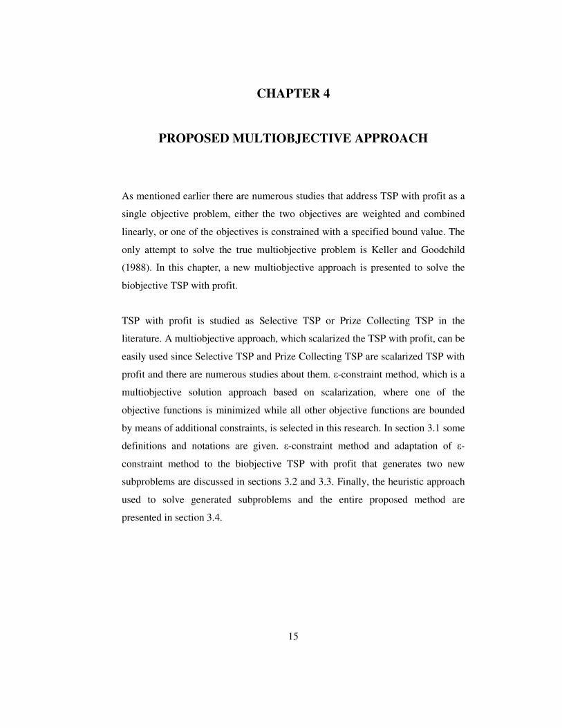
every city has to be visited. This is, however, not always realistic. Consider the

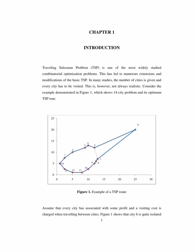
example demonstrated in Figure 1, which shows 14-city problem and its optimum

TSP tour.

Figure 1. Example of a TSP route

Assume that every city has associated with some profit and a visiting cost is

charged when travelling between cities. Figure 1 shows that city 6 is quite isolated

0

5

10

15

20

25

0 5 10 15 20 25 30

6

5 4

3

2

1

14

13 12 11 10

9 8

7

2

from the rest of the cities. A decision whether city 6 should be included in or

excluded from the route could depend on the trade-off relationship between the

profit and the visiting cost associated with city 6.

The problem in which cities are selected to be visited depending on the profit

associated with them is called Traveling Salesman Problem with Profit (TSP with

profit). TSP with profit is encountered in many different situations. For instance,

it may not be possible to visit every city in a TSP application. In this kind of

application some constraints can enforce selection of cities to be visited. Gensch

(1978) and Pekny et al. (1990) studied such problems in steel and chemical

industry, respectively. Balas and Martin (1985) introduce the scheduling of daily

operations of a steel rolling mill, which is an application of TSP with profit. This

problem gives rise to a Prize Collecting Traveling Salesman Problem (Prize

Collecting TSP) with penalty terms in the objective function.

Orienteering game is another application of TSP with profit. It is introduced by

Tsiligirides (1984). In orienteering, competitors start from a control point and

have to reach another control point within a prescribed time limit. The aim is

collecting as many points as possible within the time limit. Since it is not possible

to visit all the points, a selection of points to be visited has to be done. The

optimal route, which maximizes the points collected, is obtained by solving the

Orienteering Problem (OP).

Some other applications of TSP with profit can also be encountered in the

literature. Ramesh and Brown (1991) propose an application in control theory.

Fischetti and Toth (1988) notice that TSP with profit arises when a factory needs a

given amount of product, which can be provided by a set of suppliers with given

amounts and costs.

TSP with profit sometimes appears as subproblems in solution procedures devoted

to the different kinds of complex problems. Göthe-Lundgren et al. (1995, 1996)

3

address such subproblems in the context of vehicle routing cost allocation

problems. Noon et al. (1994) propose a heuristic procedure for the solution of

VRP, based on the iterative solution of TSP with profit.

There are varieties of TSP with profit. The two most studied problems among

them are: (i) Selective TSP (or Orienteering), (ii) Prize Collecting TSP. These

problems can be considered as the dual of each other. It can easily be recognized

that it is actually a biobjective problem where one objective is maximizing the

profit to be collected by visiting as many cities as possible, and the other objective

is keeping the visiting costs at minimum. If two objectives can be defined in

commensurable terms, then they can be combined in a single objective function

and can be solved as a single objective problem. Yet, in many cases (e.g. one

objective is maximizing the profit but the other objective is minimizing time) it is

not possible to combine two objectives. Then, a study of the trade-off relation

between two objectives may be of interest.

In literature, TSP with profit is studied as a single objective problem. The only

attempt to solve TSP with profit as a biobjective problem is done by Keller and

Goodchild (1988). The main difference of biobjective approach compared to a

single objective approach is finding not only one, but Pareto optimal solutions. By

finding more solutions, the trade-off among them can be analyzed to make better

decision. The purpose of this study is to develop a multiobjective approach for the

biobjective TSP with profit in order to obtain the Pareto optimal solutions.

The organization of the thesis is as follows: In Chapter 2, the formal definition of

the problem is presented and the mathematical representation of the problem is

given. A brief review of the related literature is presented in Chapter 3. The

related studies are classified according to solution approaches. The solution

approach is discussed in Chapter 4. �-constrained method is presented in detail

after discussing the properties of Pareto optimal solutions. In Chapter 5, the

analysis methods for the Pareto optimal solutions are discussed. In Chapter 6, the

4

performance of the �-constrained method and the results of extensive

computational experiment are presented. Chapter 7 describes the interactive

software developed for the biobjective TSP with profit. Finally, the thesis is

concluded with possible future research directions.

5

CHAPTER 2

PROBLEM DEFINITION AND MODEL

In this chapter, a formal presentation of TSP with profit is provided and the

mathematical model of the problem is presented. In section 2.1 the definition of

the problem is given and the mathematical model of the problem is given in

section 2.2.

2.1 TSP with Profit

TSP is finding the shortest route for a given number of cities. It is one of the most

widely studied combinatorial optimization problems (Guttin and Punnen 2002;

Toth and Vigo 2001). The main characteristics of TSP are that every city has to be

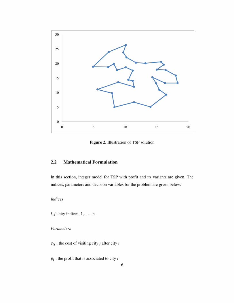
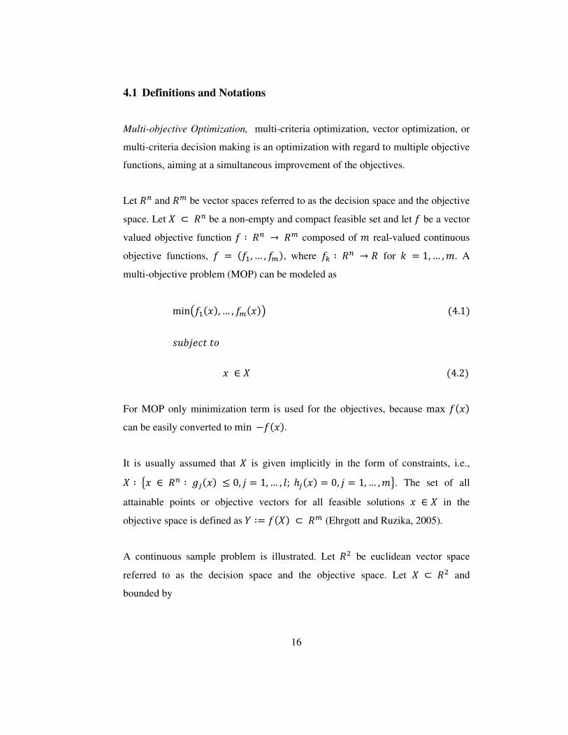
visited and no profit is associated to the cities. In Figure 2 a sample of TSP

solution is given. In this figure, the problem has 33 cities and the optimal solution

that visits each city once is shown.

A variant of TSP where a profit value is associated to each city and cities are

selected depending on their profit are proposed in the literature. Feillet et al.

(2005) define these kinds of problems as TSP with profit.

TSP with profit is actually a multiobjective problem with two conflicting

objectives, one is to collect the maximal profit and the other is to minimize the

travel cost. As a multiobjective problem, solving TSP with profit should result

non-dominated solution set, a set of feasible solutions such that neither objective

can be improved without deteriorating the other (Feillet et al. 2005).

6

Figure 2. Illustration of TSP solution

2.2 Mathematical Formulation

In this section, integer model for TSP with profit and its variants are given. The

indices, parameters and decision variables for the problem are given below.

Indices

i, j : city indices, 1, … , n

Parameters

� � : the cost of visiting city j after city i

� : the profit that is associated to city i

0

5

10

15

20

25

30

0 5 10 15 20

7

Decision Variables

� � � 1 if city j is visited after city i, 0 otherwise

� � 1 if city i is visited, 0 otherwise

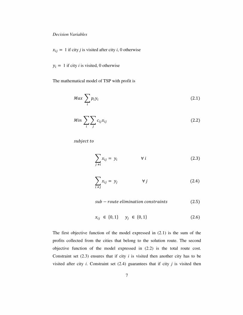
The mathematical model of TSP with profit is

�� 2.1�

�� 2.2�

�� !

�� " �� # �2.3�

�� #� " � �2.4�

�� & '!� � �(�)�� !� �!�� '�� 2.5� � � + ,0, 1. �� + ,0, 1. �2.6�

The first objective function of the model expressed in (2.1) is the sum of the

profits collected from the cities that belong to the solution route. The second

objective function of the model expressed in (2.2) is the total route cost.

Constraint set (2.3) ensures that if city i is visited then another city has to be

visited after city i. Constraint set (2.4) guarantees that if city j is visited then

8

another city has to be visited before city j. Both constraint sets (2.3) and (2.4)

ensure that if city i is arrived, then it must be leaved. Constraint set (2.5) is the set

of sub-route elimination constraints that guarantees single tour along the all cities

visited. Finally, constraint set (2.6) sets up the binary restrictions for � � and � variables.

In most of the research on TSP with profit, the problem is studied as a single

objective problem, either it is maximizing the profit and the route cost is

constrained by an upper bound or it is minimizing the route cost and the route

profit is constrained by a lower bound.

The single objective variant of TSP with profit in which the objective is

maximizing the profit is called Selective Traveling Salesman Problem (Selective

TSP). The mathematical formulation of Selective TSP is given below

�� 2.7�

�� !

�� 1 2 �2.8�

and (2.3) – (2.6)

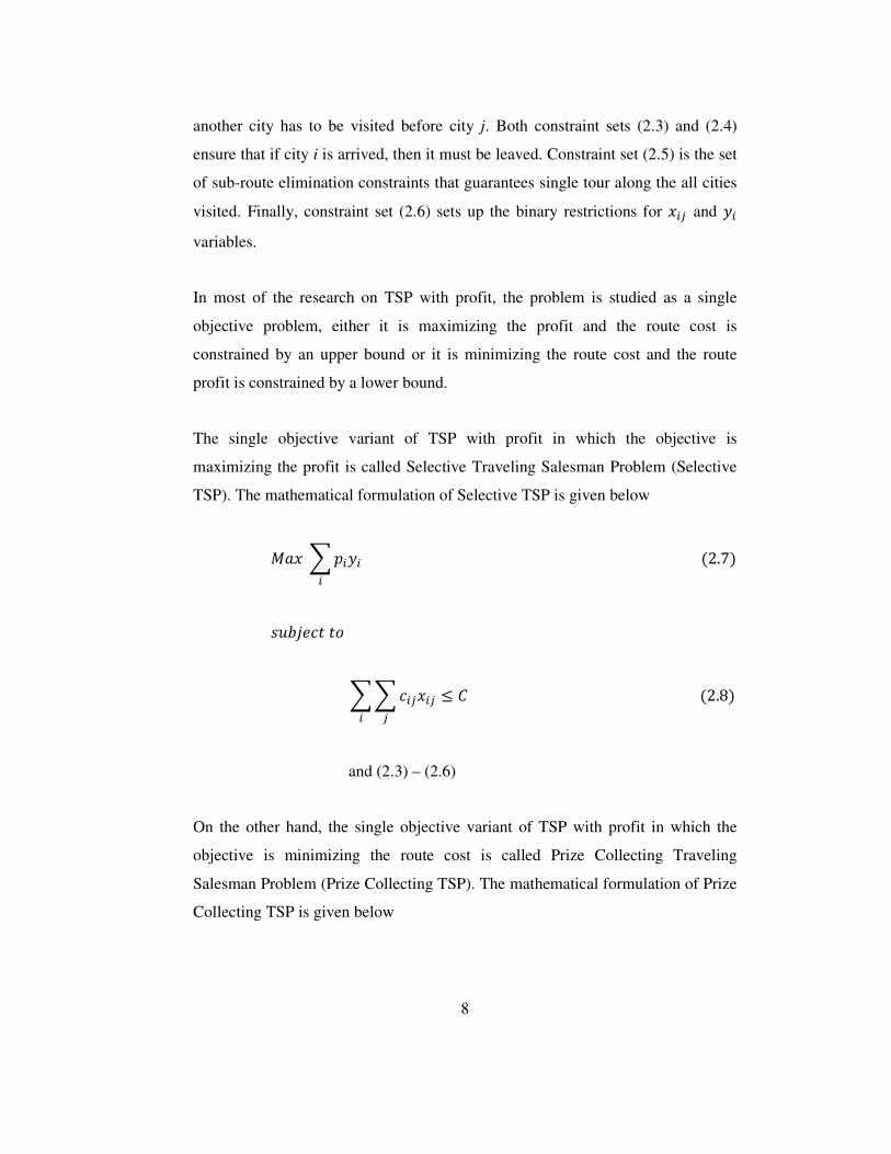
On the other hand, the single objective variant of TSP with profit in which the

objective is minimizing the route cost is called Prize Collecting Traveling

Salesman Problem (Prize Collecting TSP). The mathematical formulation of Prize

Collecting TSP is given below

9

�� 2.9�

�� !

�� 5 � �2.10�

and (2.3) – (2.6)

Intuitively, the biobjective TSP with profit is NP-hard, because TSP is NP-hard

and a TSP instance can be stated as a TSP with profit instance by defining very

large profits on vertices, therefore it is also NP-hard.

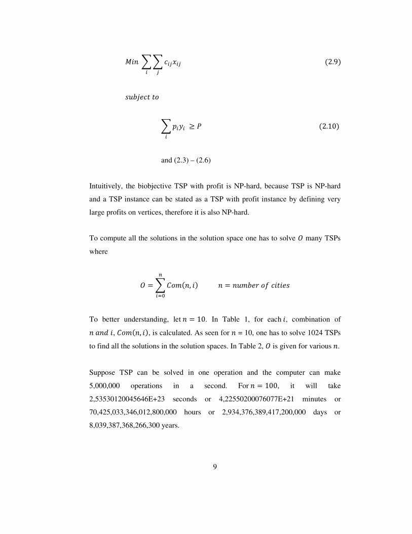
To compute all the solutions in the solution space one has to solve 6 many TSPs

where

6 � �2!)��, �� )��' !7 �� 8 9:

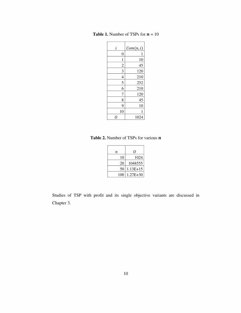
To better understanding, let � � 10. In Table 1, for each �, combination of � ��; �, 2!)��, ��, is calculated. As seen for � = 10, one has to solve 1024 TSPs

to find all the solutions in the solution spaces. In Table 2, 6 is given for various �.

Suppose TSP can be solved in one operation and the computer can make

5,000,000 operations in a second. For � � 100, it will take

2,53530120045646E+23 seconds or 4,22550200076077E+21 minutes or

70,425,033,346,012,800,000 hours or 2,934,376,389,417,200,000 days or

8,039,387,368,266,300 years.

10

Table 1. Number of TSPs for < = 10

� 2!)��, ��

0 1

1 10

2 45

3 120

4 210

5 252

6 210

7 120

8 45

9 10

10 1 6 1024

Table 2. Number of TSPs for various <

� 6

10 1024

20 1048555

50 1.13E+15

100 1.27E+30 Studies of TSP with profit and its single objective variants are discussed in

Chapter 3.

11

CHAPTER 3

LITERATURE REVIEW

The traveling salesman problem is defined as: given a finite number of cities

along with the cost of travel between each pair of them, find the cheapest way of

visiting all the cities only once and returning to your starting city. The problem

can be defined on an undirected complete graph G = (V, E), where V represents

the nodes located at the city points and the starting city, and E represents the

edges between the nodes. For every edge {i, j} + E, there is a cost � � associated

with it. We refer to the books of Gutin and Punnen (2002) and Lawyer et al.

(1985) for TSP literature.

This chapter, focusing on the well known variants of TSP, Prize Collecting TSP

and Orienteering Problem (Selective TSP), provides a literature survey of solution

approaches. These problems can be considered as the dual of each other. When we

consider them it can easily be recognized that the problem is actually biobjective

problem where the one objective is maximizing the profit to be collected by

visiting as many cities as possible, and the other objective is keeping cost to a

minimum.

In section 2.1, Selective TSP and Orienteering Problem literatures are presented

since Orienteering Problem is a special case of Selective TSP and it is more

widely studied. In section 2.2, Prize Collecting TSP literature is presented.

Finally, the only approach for the biobjective TSP with profit is presented in

section 2.3.

12

3.1 Selective TSP

There has been work on exact methods. Laporte and Martello (1990) present a

branch-and-bound scheme with linear programming (LP) relaxation. They solve

the problem where 0-1 constraints are relaxed, through linear programming and

the violated conditions are gradually solved through a branch-and-bound process.

Leifer and Rosenwein (1993) relax the 0-1 constraints and drop the connectivity

constraints. Thereafter, certain valid inequalities are added to the model. After

solving the LP relaxation, a cutting plane algorithm is added and the LP is solved

again. Fischetti et al. (1998) and Gendreau et al. (1998a) quickly tighten the

bounds with valid inequalities all along the search tree (in branch and cut

procedures). Ramesh et al. (1992) use Lagrange relaxation along with

improvement procedures within a branch and bound method. Gendreau et al.

(1998b) extend it to the insertion of clusters. Although these approaches have

yielded solutions to smaller sized problems, as in other NP-hard problems, the

computational limitations of exact algorithms encourage the exploration of

heuristic procedures.

The first heuristics, the S-algorithm and the D-algorithm, were proposed by

Tsiligirides (1984). In the S-algorithm, Tsiligirides defines a new term,

desirability measure. Points are added to the path depending on this desirability

measure. In the D-algorithm, Tsiligirides divides the area into sectors and routes

are built up within the sector. In these papers, Tsiligirides also devises the most

well known test problems for the OP, which has 21, 32 and 33 cities.

Golden, Levy and Vohra (1987) propose a procedure with three steps: path

construction using a greedy method, path improvement and center of gravity

which guides the next search step. Golden, Wang, and Liu (1988) incorporate the

center of gravity idea and desirability concepts, along with the learning

capabilities. An artificial neural network approach is proposed by Wang et al.

13

(1995). Ramesh and Brown (1991) propose a four-phase heuristic consists of node

insertion, cost improvement, node deletion and maximal insertions.

Chao, et al. (1996) introduce a two-step heuristic to solve the OP. In the first step,

initialization, by using the starting and ending nodes as the two foci of an ellipse

and the route cost constraint as the length of the major axis, several routes are

generated and the one with the highest score is the initial solution. The initial

route is then improved by a 2-node exchange in the cheapest-cost way, and then

improved by a 1-node improvement that tries to increase the total score. They

apply this algorithm to Tsiligirides (1984) problems and 40 new test problems.

The authors also point out a mistake in Tsiligirides data set and suggest the

correction.

Tasgetiren and Smith (2000) propose a genetic algorithm (GA) to solve the

orienteering problem. Four test sets, the three originally from Tsiligirides (1984)

and the one corrected by Chao, et al. (1996), are used. Tasgetiren results are

competitive to the best known heuristics, though the computational time is

relatively high. Liang and Smith (2001) recently proposed a standard ant colony

algorithm, hybridized with local search, for the OP. They apply this algorithm to

Tsiligirides (1984) problems and the one corrected by Chao, et al. (1996). Their

results are competitive to the best known heuristics, too.

3.2 Prize Collecting TSP

“PCTSP was introduced by Balas and Martin (1985) as a model for scheduling

the daily operations of a steel rolling mill and the same optimization problem was

successively addressed by Balas and Martin (1991). Also, structural properties of

the PCTSP related to the TSP polytope and to the knapsack polytope were

presented by Balas (1989) and Balas (1995).” (Dell’Amico et al. 1998)

14

Fischetti and Toth (1988) use a Lagrangian relaxation for the generalized covering

constraint and solve assignment problem which is resulted by a subtour relaxation.

The solution of this assignment problem provides a bound. Dell’Amico et al.

(1995) also uses bounding procedure based on different relaxation. Bienstock et

al. (1993) studied undirected Prize Collecting TSP. They use linear programming

relaxation. Goemans and Williamson (1995) improve the above algorithm. Göthe-

Lundgren et al. (1995) propose another approach based on Lagrangian

decomposition to obtain a bound. Balas (1999) introduces ordering constraints for

which the PCTSP becomes polynomially solvable. In the same way, Kabadi and

Punnen (1996) extend results on polynomially solvable cases of the TSP to the

PCTSP.

Dell’Amico et al. (1998) present two heuristic procedures for the PCTSP. In the

first one, the Lagrangian relaxation is used for route construction. Insertion is then

used to attain feasibility of the route. Afterward, extension and collapse are

applied iteratively to improve the route. Extension applies insertion as long as

insertions are over a computed average ratio. Collapse carries out the replacement

of a chain by a single vertex. The second heuristic uses the same components, but

in a different order.

3.3 The Biobjective TSP with Profit

The only study for the biobjective TSP with profit is Keller and Goodchild (1988).

They uses Tsiligirides’ (1984) algorithm for the multi-objective vending problem

(MVP) to solve the OP. A path construction phase uses a measure identical to that

of the S-algorithm. This is followed by a three step improvement phase that uses

node insertion and identification of node clusters. They used 25 cities located in

West Germany. Bonn was used as the depot and terminal node. The populations

of cities were treated as profit associated with each city.

15

CHAPTER 4

PROPOSED MULTIOBJECTIVE APPROACH

As mentioned earlier there are numerous studies that address TSP with profit as a

single objective problem, either the two objectives are weighted and combined

linearly, or one of the objectives is constrained with a specified bound value. The

only attempt to solve the true multiobjective problem is Keller and Goodchild

(1988). In this chapter, a new multiobjective approach is presented to solve the

biobjective TSP with profit.

TSP with profit is studied as Selective TSP or Prize Collecting TSP in the

literature. A multiobjective approach, which scalarized the TSP with profit, can be

easily used since Selective TSP and Prize Collecting TSP are scalarized TSP with

profit and there are numerous studies about them. ε-constraint method, which is a

multiobjective solution approach based on scalarization, where one of the

objective functions is minimized while all other objective functions are bounded

by means of additional constraints, is selected in this research. In section 3.1 some

definitions and notations are given. ε-constraint method and adaptation of ε-

constraint method to the biobjective TSP with profit that generates two new

subproblems are discussed in sections 3.2 and 3.3. Finally, the heuristic approach

used to solve generated subproblems and the entire proposed method are

presented in section 3.4.

16

4.1 Definitions and Notations

Multi-objective Optimization, multi-criteria optimization, vector optimization, or

multi-criteria decision making is an optimization with regard to multiple objective

functions, aiming at a simultaneous improvement of the objectives.

Let =8 and => be vector spaces referred to as the decision space and the objective

space. Let � ? =8 be a non-empty and compact feasible set and let 7 be a vector

valued objective function 7 @ =8 A => composed of ) real-valued continuous

objective functions, 7 � �7B, … , 7>�, where 7D @ =8 A = for E � 1,… ,). A

multi-objective problem (MOP) can be modeled as

minI7B��, … , 7>��J �4.1�

�� ! � + � �4.2�

For MOP only minimization term is used for the objectives, because max 7��

can be easily converted to min &7��. It is usually assumed that � is given implicitly in the form of constraints, i.e.,

� @ M� + =8 @ N�� 1 0, � � 1,… , (; P�� 0, � � 1,… ,)Q. The set of all

attainable points or objective vectors for all feasible solutions � + � in the

objective space is defined as R @� 7�� ? => (Ehrgott and Ruzika, 2005).

A continuous sample problem is illustrated. Let =S be euclidean vector space

referred to as the decision space and the objective space. Let � ? =S and

bounded by

17

3�B T �S 5 12

�B T 3�S 5 12

�B T �S 5 9

Let 7 � �7B, 7S� where 7B�� B and 7S�� S.

This simple MOP (S3.1) can be modeled as

min �B

min �S

�� ! 3�B T �S 5 12 �4.3�

�B T 3�S 5 12 �4.4�

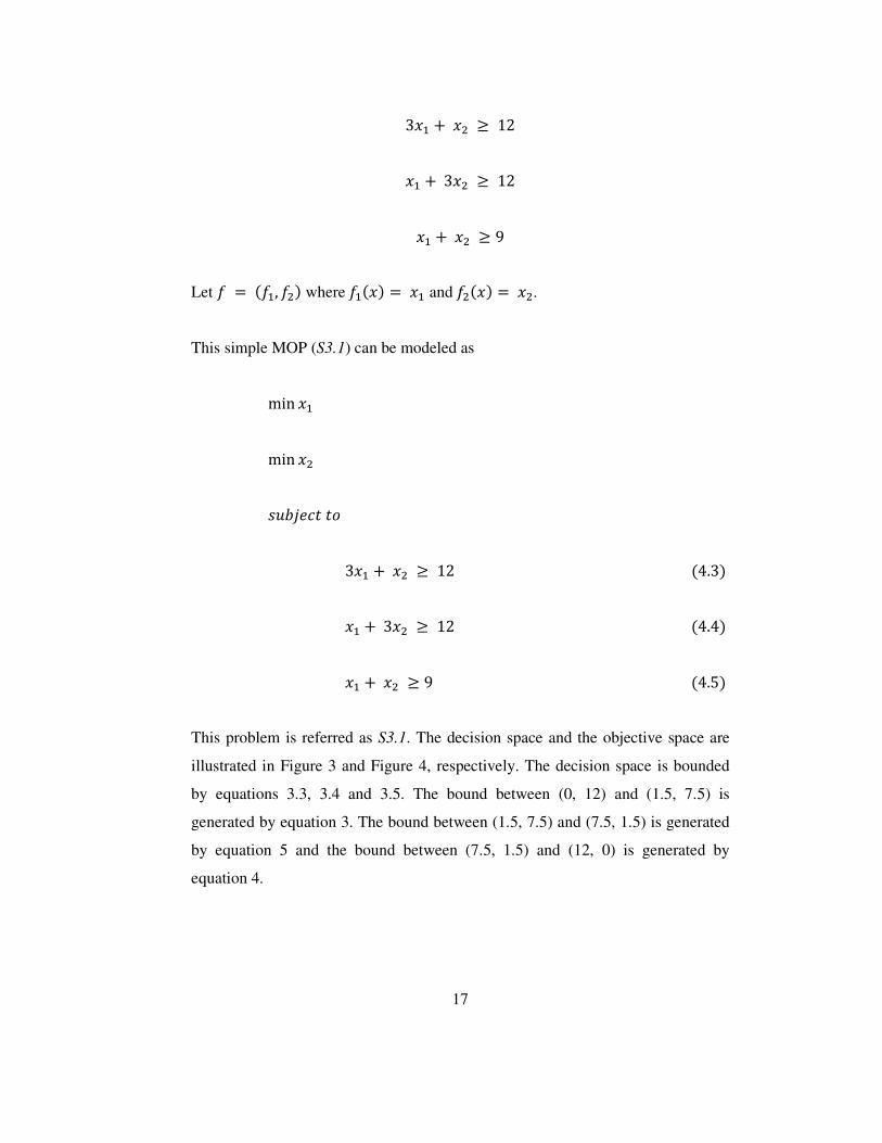
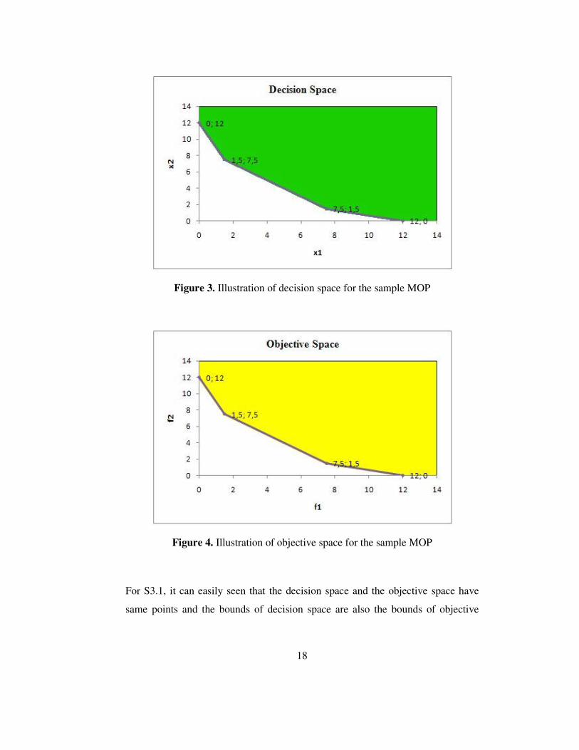
�B T �S 5 9 �4.5� This problem is referred as S3.1. The decision space and the objective space are

illustrated in Figure 3 and Figure 4, respectively. The decision space is bounded

by equations 3.3, 3.4 and 3.5. The bound between (0, 12) and (1.5, 7.5) is

generated by equation 3. The bound between (1.5, 7.5) and (7.5, 1.5) is generated

by equation 5 and the bound between (7.5, 1.5) and (12, 0) is generated by

equation 4.

18

Figure 3. Illustration of decision space for the sample MOP

Figure 4. Illustration of objective space for the sample MOP

For S3.1, it can easily seen that the decision space and the objective space have

same points and the bounds of decision space are also the bounds of objective

19

space, since 7B�� B and 7S�� S. But this is not the case for most of the

MOPs and it is hard to find the bounds for the objective space.

The objective functions are usually conflicting in MOPs. As the objective function

contradicts, no point can be optimal for all ) objective functions simultaneously.

Thus the optimality concept used in scalar optimization must be replaced by a

new one, called Pareto Optimality.

Pareto Optimality is an optimality criterion for MOPs. A solution xU is said to be

Pareto optimal, if there is no other solution xV dominating the solution xU with

respect to a set of objective functions. A solution xU dominates a solution xV, if xU

is better than xV in at least one objective function and not worse with respect to

all other objective functions.

�W + X is Pareto optimal if and only if there exists no �Y + X such that 7D��Y� 1 7D��W� for all E � 1,… ,) with 7D��Y� Z 7D��W� for at least one E.

�W + X dominates �Y + X if and only if 7D��W� 1 7D��Y� for all E � 1,… ,)

with 7D��W� Z 7D��Y� for at least one E.

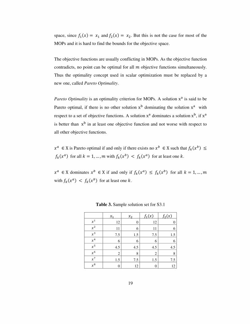
Table 3. Sample solution set for S3.1

�B �S 7B�� 7S�� B 12 0 12 0 �S 11 6 11 6 �[ 7.5 1.5 7.5 1.5 �\ 6 6 6 6 �] 4.5 4.5 4.5 4.5 �^ 2 8 2 8 �_ 1.5 7.5 1.5 7.5 �` 0 12 0 12

20

For the sample solution given in Table 3, dominations and Pareto optimality is

explained below.

�[ dominates �2 since 7.5 Z 11 and 1.5 < 6.

�\ dominates �2 since 6 � 6 and 6 < 11.

�] dominates �4 since 4.5 Z 6 and 4.5 < 6.

�] also dominates �2.

�_ dominates �6 since 1.5 Z 2 and 7.5 < 8.

�B is also Pareto optimal, since there is no solution that dominates �B.

For the sample solution set, solutions �S, �\ and �^ are dominated by

solutions �[, �] and �_, respectively. Solutions �B, �[, �], �_ and �` are Pareto

optimal, since there is no solution that dominates these solutions. Pareto optimal

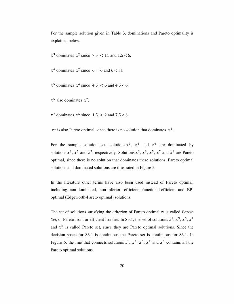
solutions and dominated solutions are illustrated in Figure 5.

In the literature other terms have also been used instead of Pareto optimal,

including non-dominated, non-inferior, efficient, functional-efficient and EP-

optimal (Edgeworth-Pareto optimal) solutions.

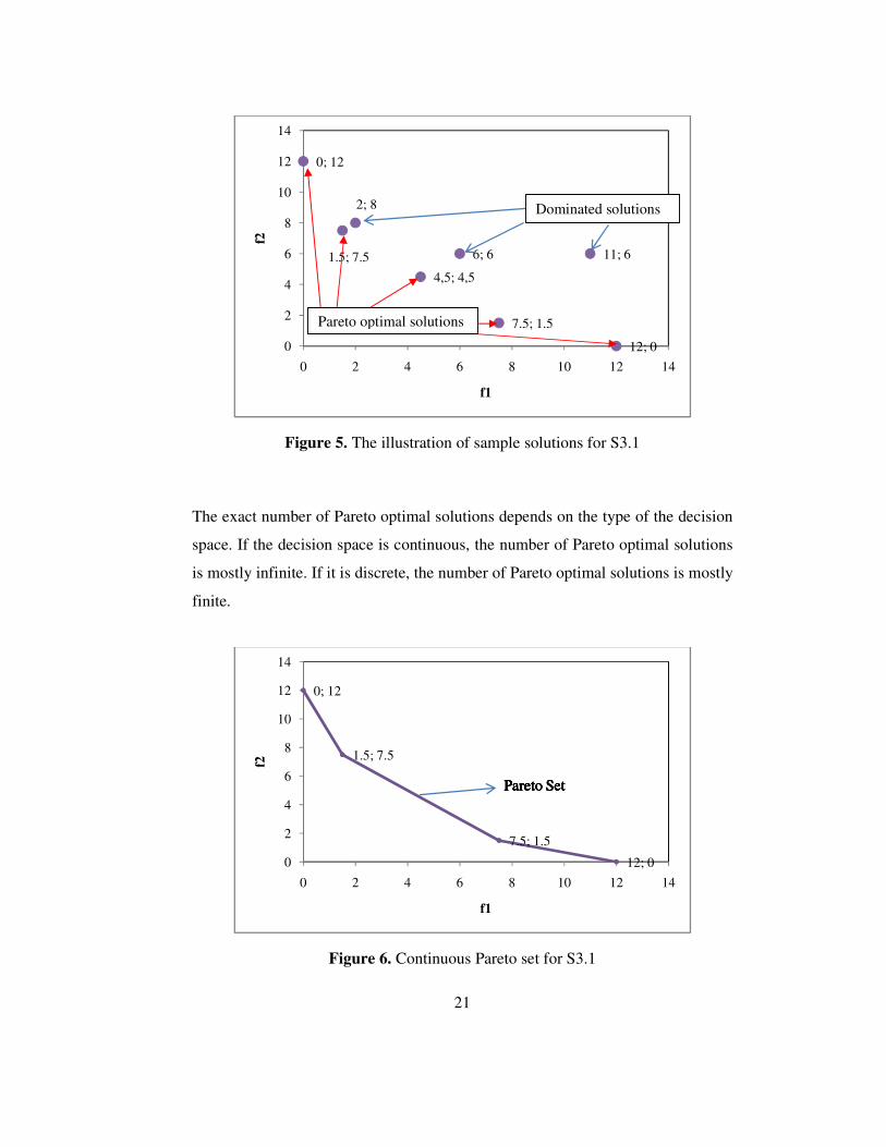
The set of solutions satisfying the criterion of Pareto optimality is called Pareto

Set, or Pareto front or efficient frontier. In S3.1, the set of solutions �B, �[, �], �_

and �` is called Pareto set, since they are Pareto optimal solutions. Since the

decision space for S3.1 is continuous the Pareto set is continuous for S3.1. In

Figure 6, the line that connects solutions �B, �[, �], �_ and �` contains all the

Pareto optimal solutions.

21

Figure 5. The illustration of sample solutions for S3.1

The exact number of Pareto optimal solutions depends on the type of the decision

space. If the decision space is continuous, the number of Pareto optimal solutions

is mostly infinite. If it is discrete, the number of Pareto optimal solutions is mostly

finite.

Figure 6. Continuous Pareto set for S3.1

12; 0

11; 6

7.5; 1.5

6; 6

4,5; 4,5

2; 8

1.5; 7.5

0; 12

0

2

4

6

8

10

12

14

0 2 4 6 8 10 12 14

f2

f1

0; 12

1.5; 7.5

7.5; 1.5

12; 00

2

4

6

8

10

12

14

0 2 4 6 8 10 12 14

f2

f1

Pareto SetPareto SetPareto SetPareto SetPareto SetPareto Set

Dominated solutions

Pareto optimal solutions

22

For a discrete decision space Pareto set may be illustrated as in Figure 7.

Figure 7. Illustration of discrete Pareto set

4.2 ε-constraint Method

The ε-constraint method is a multi-objective optimization technique, proposed by

Haimes et al. (1983), for generating Pareto optimal solutions. It is based on a

scalarization where one of the objective functions is choosen as a scalar objective

to be minimized and other objective functions are transformed into constraints.

For transforming the multi-objective problem into several single-objective

problems with constraints, it uses the following procedure.

min 7D�� 4.6�

�� !

0

10

20

30

40

50

60

70

80

90

100

0 20 40 60 80 100

f2

f1

23

7 �� 1 � � a E �4.7�

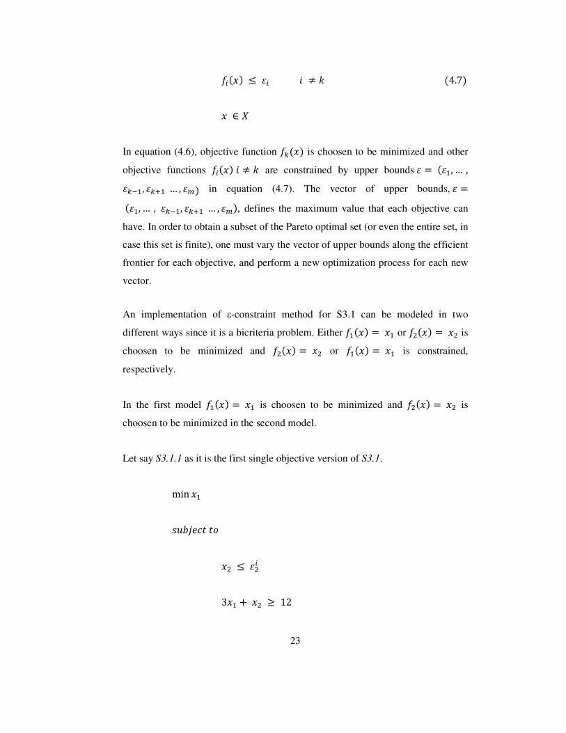
� + � In equation (4.6), objective function 7D�� is choosen to be minimized and other

objective functions 7 �� a E are constrained by upper bounds � � ��B, … ,�DbB, �DcB … , �>� in equation (4.7). The vector of upper bounds, � � ��B, … , �DbB, �DcB … , �>�, defines the maximum value that each objective can

have. In order to obtain a subset of the Pareto optimal set (or even the entire set, in

case this set is finite), one must vary the vector of upper bounds along the efficient

frontier for each objective, and perform a new optimization process for each new

vector.

An implementation of ε-constraint method for S3.1 can be modeled in two

different ways since it is a bicriteria problem. Either 7B�� B or 7S�� S is

choosen to be minimized and 7S�� S or 7B�� B is constrained,

respectively.

In the first model 7B�� B is choosen to be minimized and 7S�� S is

choosen to be minimized in the second model.

Let say S3.1.1 as it is the first single objective version of S3.1.

min �B

�� ! �S 1 �S

3�B T �S 5 12

24

�B T 3�S 5 12 �B T �S 5 9

Let say S3.1.2 as it is the second single objective version of S3.1.

min �S

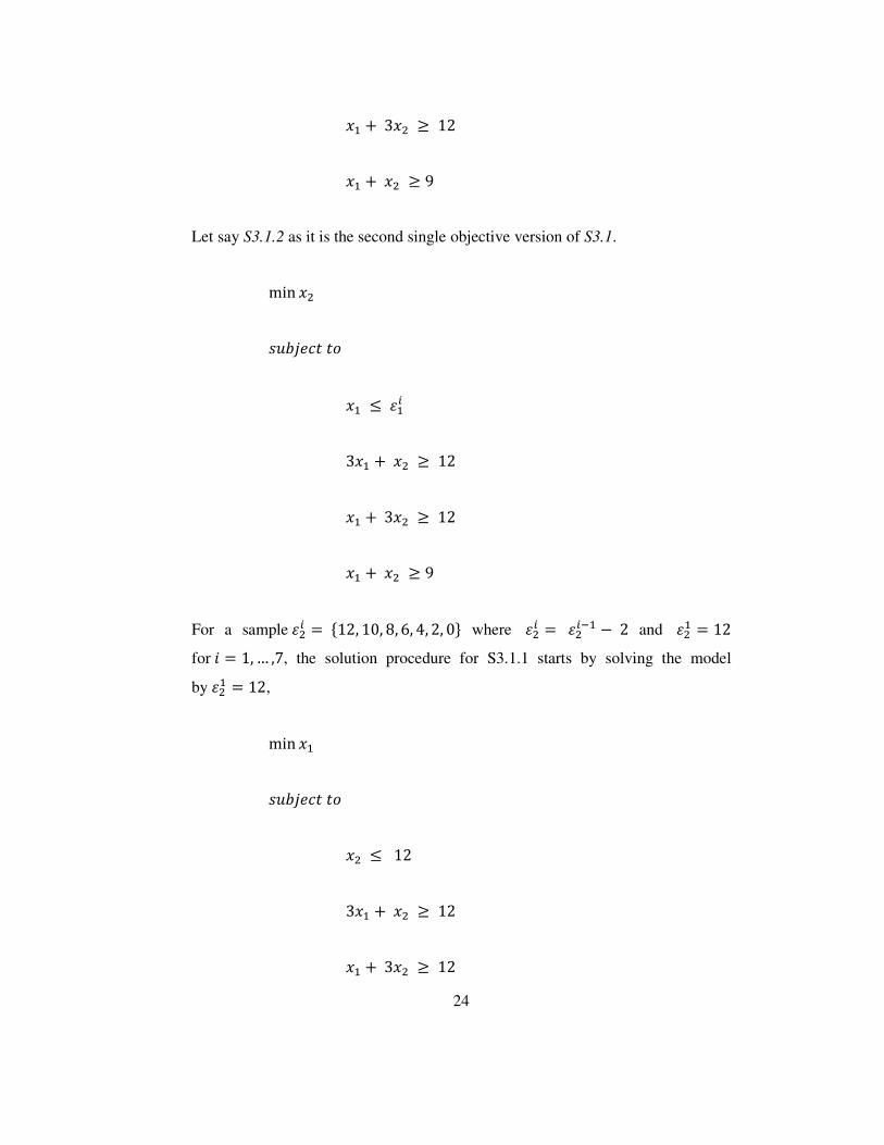
�� ! �B 1 �B 3�B T �S 5 12 �B T 3�S 5 12 �B T �S 5 9

For a sample �S � ,12, 10, 8, 6, 4, 2, 0. where �S � �S bB & 2 and �SB � 12

for � � 1,… ,7, the solution procedure for S3.1.1 starts by solving the model

by �SB � 12,

min �B

�� ! �S 1 12

3�B T �S 5 12 �B T 3�S 5 12

25

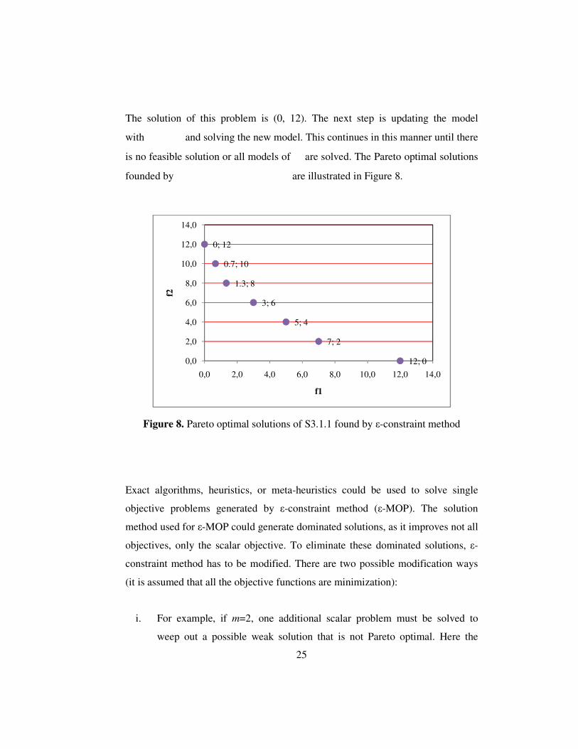
The solution of this problem is (0, 12). The next step is updating the model

with and solving the new model. This continues in this manner until there

is no feasible solution or all models of are solved. The Pareto optimal solutions

founded by are illustrated in Figure 8.

Figure 8. Pareto optimal solutions of S3.1.1 found by ε-constraint method

Exact algorithms, heuristics, or meta-heuristics could be used to solve single

objective problems generated by ε-constraint method (ε-MOP). The solution

method used for ε-MOP could generate dominated solutions, as it improves not all

objectives, only the scalar objective. To eliminate these dominated solutions, ε-

constraint method has to be modified. There are two possible modification ways

(it is assumed that all the objective functions are minimization):

i. For example, if m=2, one additional scalar problem must be solved to

weep out a possible weak solution that is not Pareto optimal. Here the

0; 12

0.7; 10

1.3; 8

3; 6

5; 4

7; 2

12; 00,0

2,0

4,0

6,0

8,0

10,0

12,0

14,0

0,0 2,0 4,0 6,0 8,0 10,0 12,0 14,0

f2

f1

26

earlier constrained objective is put into the objective function and the

former objective function is removed to form an equality constraint where

the allowable limit is the optimum solution of the first problem.

ii. The constrained objectives are added to the scalar objective by a set of

appropriate weights. The objective function equals to the sum of Ede

objective function and the negative weighted constrained objectives.

The first modification needs more computations as there are subproblems needed

to solve. The second modification is choosen in order to eliminate dominated

solution in our implementation. The ε-constraint method algorithm is given in

Figure 9.

Figure 9. ε-constraint method algorithm

Step 1. Set Pareto Set � f, ( � 0

Step 2. Choose the Ede objective, 7D��, to be minimized,

Step 3. Initialize � � ��B, … , �DbB, �DcB … , �>� Step 4. Constrain objectives 7 �� a E by using upper bounds �

Step 5. Solve ε-MOP

Step 6. Set g � solution of ε-MOP. If there is no feasible solution, then stop

Step 7. Set g + Pareto Set

Step 8. Set ( � ( T 1

Step 9. Update �, return Step 4

27

4.3 Adaptation of ε-constraint Method

Implementation of the ε-constrained method to the biobjective TSP with profit

arises two different problems depending on the main single objective:

• The objective is increasing the profit while the route cost is upper bounded

as an additional constraint

• The objective is decreasing the route cost while the profit is lower

bounded as an additional constraint

The first problem is known as STSP, or Orienteering Problem, as discussed

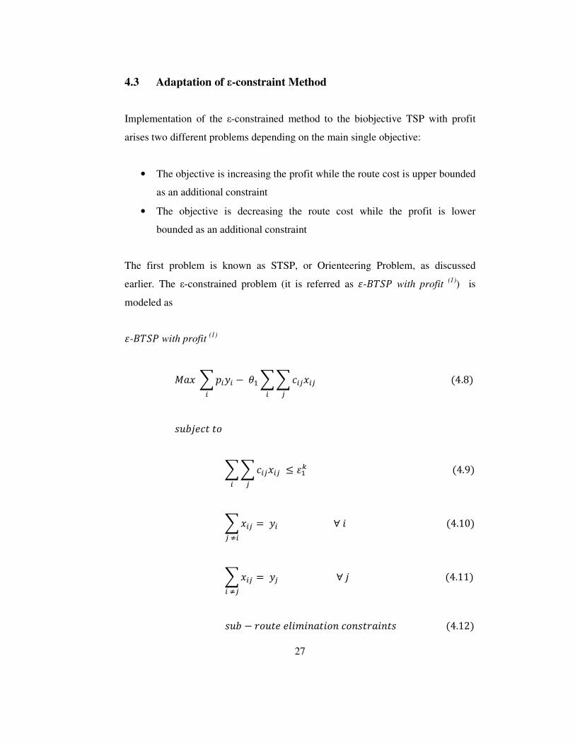
earlier. The ε-constrained problem (it is referred as �-�� with profit (1)) is

modeled as

�-�� with profit (1)

�� & hB �� 4.8��

�� !

�� 1 �BD �4.9�

�� " �� # �4.10�

�� #� " � �4.11�

�� & '!� � �(�)�� !� �!�� '�� 4.12�

28

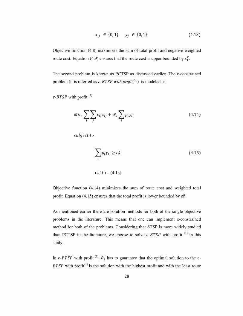
� � + ,0, 1. �� + ,0, 1. �4.13�

Objective function (4.8) maximizes the sum of total profit and negative weighted

route cost. Equation (4.9) ensures that the route cost is upper bounded by �BD.

The second problem is known as PCTSP as discussed earlier. The ε-constrained

problem (it is referred as �-�� with profit (2)) is modeled as

�-�� with profit (2)

�� T hS �� 4.14� �� !

�� 5 �SD �4.15� (4.10) – (4.13)

Objective function (4.14) minimizes the sum of route cost and weighted total

profit. Equation (4.15) ensures that the total profit is lower bounded by �SD.

As mentioned earlier there are solution methods for both of the single objective

problems in the literature. This means that one can implement ε-constrained

method for both of the problems. Considering that STSP is more widely studied

than PCTSP in the literature, we choose to solve �-�� with profit (1) in this

study.

In �-�� with profit (1), hB has to guarantee that the optimal solution to the �-�� with profit(1) is the solution with the highest profit and with the least route

29

cost if there exist any other solutions with the highest profit. Let 2>Wi �maxM� �Q, 2> 8 � minM� �Q and ��: � � j 2>Wi. It is natural that 2> 8 is

the lower bound and ��: is the upper bound for the route cost. Let �B be the

maximum profit gained for the �-�� with an upper bound ��:. Let ��: 5 ��B 5 ��S.

�B & hB j ��S 5 �B & hB j ��B �4.16�

hB 1 ��B ��S⁄

Let 7S��B, ��S� be the solution with profit �B and cost ��S and 7B��B, ��B� be the solution with profit �B and cost ��B. Expression (4.16)

implies that 7S��B, ��S� dominates 7B��B, ��B�. Then the solution of the �-�� has to be 7S��B, ��S� which means that the objective function value of 7S��B, ��S� would be higher than the objective function value of 7B��B, ��B� as written in equation (4.16). If hB 1 ��B ��S⁄ , it is

guaranteed that among the solutions with the same profit, the solution with the

least route cost is chosen.

On the other hand, hB also has to satisfy that the solution with the highest profit is

choosen instead of the solution with the lower profit but also the lower route cost.

Let �S be the profit gained for Pareto optimal solution where the route cost is ��: and �S & P, where P is a integer small number (Let P � 1), be the profit

for the solution with the lower route cost, 2> 8. hB also satisfies equation (4.17)

�S & hB j ��: 5 �S & P & hB j 2> 8 �4.17� hB 1 P ��: & 2> 8�⁄

30

Lower and upper bounds used in equation (4.17) to obtain hB that guarantee for

any route cost, the solution with the highest profit is chosen. Since 1 ��:⁄ 1P ��: & 2> 8�⁄ , hB � 1 ��:⁄ could be used.

In �-�� with profit (1), there is only one constrained objective, upper bounded

by �BD = �BDbB & �. For E � 0, �B: � ��: since ��: is the upper bound for

route cost, there is no route whose cost higher than ��:. Since �B: is obtained,

one can calculate other �BD where E � 1,… , l depending on �. There is no way to

obtain a value of � such that every Pareto optimal solutions are found. In this

study � � 0.0001 is choosen.

The ε-constraint method algorithm for the biobjective TSP with Profit is given in

Figure 10.

The performance of the ε-constraint method depends on the method used to solve

the ε-MOP (ε-BTSP in this study). The ε-constraint method only guarantees to

obtain exact Pareto optimal solutions if the solution methodology of �-��

(SM�-��) can find the global optimum of the ε-constraint problem. Otherwise,

Pareto optimal solutions found by ε-constraint method are near Pareto optimal

solutions. Also, the number of Pareto optimal solutions depends on not only ε, but

on SMε-BTSP. In literature, there are good SMε-BTSPs for ε-BTSP. The best

SMε-BTSPs are of Ramesh and Brown (1991), Chao et al. (1996a), Golden et al.

(1988) and Wang et al. (1995) as discussed in Chapter 3.

CGW heuristic is developed by Chao et al. (1996a) and it is simple, fast, and

effective heuristic. The results of CGW heuristic are the best results obtained so

far in the literature (Tasgetiren and Smith, 2000). Therefore, CGW heuristic is

used as SMε-BTSP for ε-BTSP in this study.

31

Figure 10. ε-constraint method algorithm for r-stuv with profit (1)

4.4 CGW Heuristic Method

CGW heuristic basically consists of initialization and improvement steps. In the

initilization step, L solutions are generated by a greedy method. In the

improvement step, first, two-point exchange is applied to the initial solution on a

record-to-record improvement basis. Then one point movement is applied to the

Step 1. Set Pareto Set � f, ( � 0

Step 2. Define 2>Wi and set ��: � � j 2>Wi

Step 3. Set hB � 1 ��:⁄ , �B: � ��:, � � 0.0001

Step 4. Set objective function as ∑ � � & hB ∑ ∑ � ��

Step 5. Add ∑ ∑ � �� 1 �Bg as a constraint to form �-�� with profit (1)

Step 6. Solve �� with profit (1)

Step 7. Set g � solution of �� with profit (1). If there is no feasible

solution, then stop


Step 9. Set ( � ( T 1

Step 10.Calculate �Bg = �BgbB & �, return Step 5

32

current solution generated by two-point exchange procedure. Finally, 2-opt

procedure is applied to the current solution to decrease the length of the current

solution (Taşgetiren et al., 2002). This procedure is repeated until � loops. At the

end of � loops reinitialization step is applied. The loop that contains M loops and

reinitialization step is repeated until K loops. The best tour found so far is the

result of the heuristic.

In sections 4.4.1 and 4.4.2, set-up process and initilization of the heuristic in

which paths constructions are done in a greedy way are discussed. In sections,

4.4.3, 4.4.4 and 4.4.5, improvement steps, two-point exchange, one point

movement, and 2-opt are described, respectively. Finally, re-initialization step is

discussed in section 4.4.6.

4.4.1 Set – Up Process of CGW

Let � be the number of cities for a given problem instance and �: be starting city

and �8bB be ending city. Let �>Wi be the upper bound for the constrained

objective function, ∑ ∑ � �� and ;��, �� be the distance between cities � and �, � and ��. The procedure is initialized by calculating the sum of distances of the

city � to �: and �8bB, ; , for all � a 0, � & 1, where

; � ;��, 0� T ;��, � & 1�

Cities where ; 1 �>Wi for all � a 0, � & 1 are used for the next steps of

heuristic and cities where ; x �>Wi for all � a 0, � & 1 are eliminated.

In other words, if �: a �8bB, an ellipse is constructed over the entire set of cities

by using starting and ending cities as the foci of the ellipse and the upper bound �>Wi as the length of the major axis, as seen in Figure 11. If �: � �8bB, a circle

is constructed over the entire set of cities by using starting (ending) city as the

center of the circle and the upper bound �>Wi as the diameter of the circle, as seen

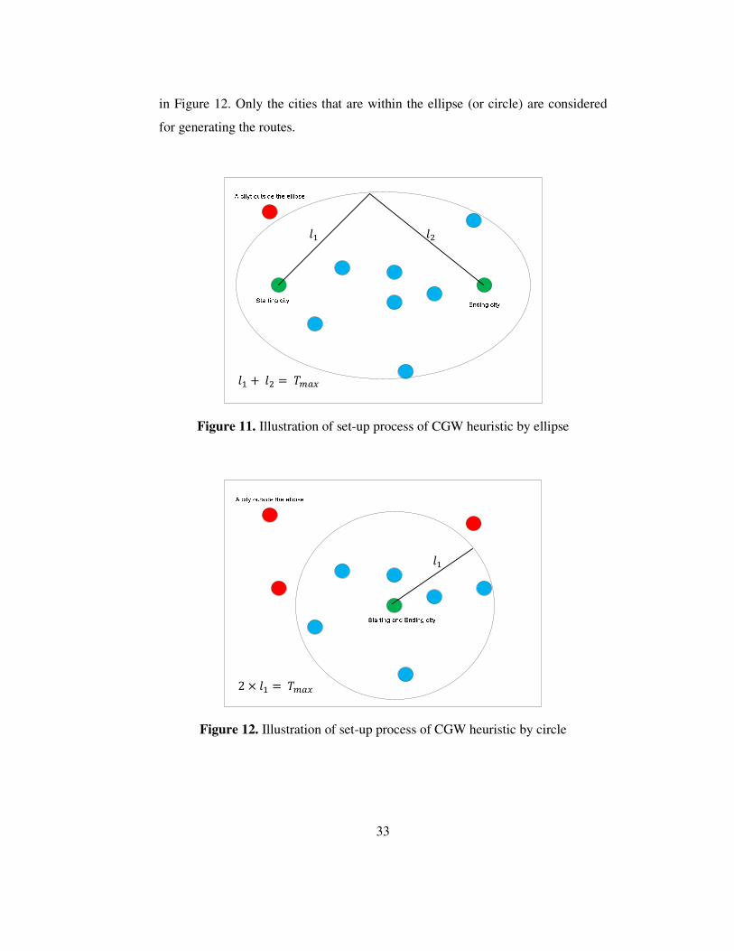
33

in Figure 12. Only the cities that are within the ellipse (or circle) are considered

for generating the routes.

Figure 11. Illustration of set-up process of CGW heuristic by ellipse

Figure 12. Illustration of set-up process of CGW heuristic by circle

(B (S

(B T (S � �>Wi

(B

2 j (B � �>Wi

34

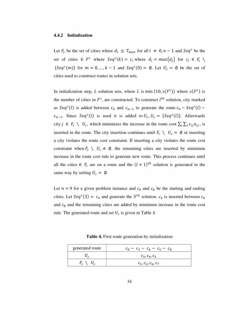
4.4.2 Initialization

Let yz be the set of cities where ; 1 �>Wi for all � a 0, � & 1 and �{z be the

set of cities + yz where �{z�E� � � where ; � )��M;�Q for �� + yz | ,�{z�)�. for ) � 0,… , E & 1 and �{z�0� � f. Let }z � f be the set of

cities used to construct routes in solution sets.

In initialization step, ~ solution sets, where ~ is min �10, ��yz�� where ��yz� is

the number of cities in yz, are constructed. To construct (de solution, city marked

as �{z�(� is added between �: and �8bB to generate the route �: & �{z�(� &�8bB. Since �{z�(� is used it is added to }z, }z � ,�{z�(�.. Afterwards

city � + yz | }z, which minimizes the increase in the route cost ∑ ∑ � �� , is

inserted in the route. The city insertion continues until yz | }z � f or inserting

a city violates the route cost constraint. If inserting a city violates the route cost

constraint when yz | }z a f, the remaining cities are inserted by minimum

increase in the route cost rule to generate new route. This process continues until

all the cities + yz are on a route and the �( T 1�de solution is generated in the

same way by setting }z � f.

Let � � 9 for a given problem instance and �: and �` be the starting and ending

cities. Let �{z�3� � �\ and generate the 3�� solution. �\ is inserted between �:

and �` and the remaining cities are added by minimum increase in the route cost

rule. The generated route and set }z is given in Table 4.

Table 4. First route generation by initialization

generated route �: & �[ & �\ & �] & �` }z �[, �\, �] yz | }z �B, �S, �^, �_

35

As yz | }z a f and route cost constraint is violated, remaining cities are

inserted between �: and �` to generate new routes. 3 solutions (solution set 3) are

given in Table 5.

Table 5. Solution set 3

generated route 1 �: & �[ & �\ & �] & �`

generated route 2 �: & �B & �S & �`

generated route 3 �: & �^ & �_ & �`

Among ~ solution sets generated by initialization process, the solution set which

has the highest objective value, ∑ � � & hB ∑ ∑ � �� , is choosen as the initial

set of routes and the objective value is set as Record. Within the initial solutions,

the route with the highest objective value is denoted as routeop and the other

routes are denoted as routenop.

4.4.3 Two-point Exchange

Chao et al. (1996) apply two-city exchange procedure to improve routeop. A city i

is selected from routeop and inserted into one of the routes in routenop and a city j

is selected from one of the routes in routenop and inserted into routeop. The

selection of cities is done arbitrary. The insertions are performed by considering

the minimum increase in route cost rule, and the feasibility of routes is

maintained. If any city insertion is not possible in routenop then a new route that

includes city i, has to be generated and added to routenop. If the objective function

value associated with a route in routenop has a higher value than the objective

function value of routeop, routeop is updated and the previous routeop is placed into

routenop.

36

Let 'B be the initial route and 'S be the updated route obtained by removing city

) and inserting city �. Let ∑ ∑ � �� B be the route cost associated with 'B. To

check the route feasibility of 'S the following expression is used.

�� B & �;I�>, ��J T ;I�>, ��J & ;I�� , ��J�T )��D9B,8M;I�8, ��J T ;��8, �D� & ;I�D, ��JQ �4.18�

where �� is the city precedes city ), �� is the city follows city m and �� is the

city precedes city k. If the distance calculated by Expression (12) is less

than �>Wi, then the generated route is feasible; otherwise, it is infeasible. In

expression (4.18), �;I�>, ��J T ;I�>, ��J & ;I�� , ��J� is the savings by

removing city ) and )��D9B,8M;I�8, ��J T ;��8, �D� & ;I�D , ��JQ is the cost

incurred by inserting city � onto path 'B.

If the city exchange increases the objective function value, the exchange is

performed immediately. On the other hand, if there is no city exchange that

increases the objective function value, then the exchanges that decrease the

objective function value by acceptable amounts are considered and the city

exchange that results the minimum decrease in the objective function value is

performed. This approach is based on record-to-record improvement (Dueck,

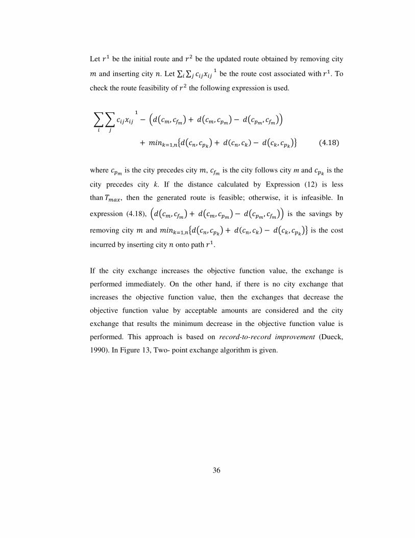
1990). In Figure 13, Two- point exchange algorithm is given.

37

Figure 13. Two-point exchange algorithm

Step 1. Set the route with the highest objective funtion value = routeop

Step 2. Set other routes = routenop

Step 3. Set the �� Y��d_�izeW8�� 0 and '��!';Y��d_�izeW8�� 0

Step 4. For m = the first to the last city in routeop

Step 5. For n = the first to the last city in the first to the last route in routenop

Step 6. If exchanging city m and city n is feasible and the objective function

value increases, then do the exchange and go step 6.1, else go step 7

Step 6.1 If the objective function value associated with a route in

routenop has a higher value than the objective function value of

routeop, then update routeop, routenop and '��!'; and go step 4,

else go step 7

Step 7. If the objective function value 5 '��!';Y��d_�izeW8��

Step 7.1 Set �� Y��d_�izeW8�� and

'��!';Y��d_�izeW8�� the objective function value

Step 8. If � � number of cities in routenop, then go step 9, else go step 5

Step 9. If '��!';Y��d_�izeW8�� 5 10% j '��!';, then exchange city )

with �� Y��d_�izeW8�� and update routeop and routenop and set

�� Y��d_�izeW8�� 0 and '��!';Y��d_�izeW8�� 0

Step 10. If ) � number of cities in routeop, then exit, else go step 4

38

4.4.4 One Point Movement

In one point movement, one city is moved from one route to other route at a time

and movement is performed by the first feasible insertion rule. City i within the

ellipse or circle is inserted between cities in the first edge of route r, then the

second edge of path p, and so on, where route r is a route that does not contain

city i. The movement is performed whenever it is feasible, it is referred as first

feasible insertion rule, and the objection function value increases. If there is no

movement that increases the objection function value, then the city movements

that decrease the route profit by acceptable amounts are considered and the city

movement that has the minimum decrease in the objection function value is

performed. The feasibility of insertion is checked by Equation (4.19).

�� & �;I�>, ��J T ;I�>, ��J & ;I�� , ��J�T �;I�8, ��J T ;��8, �D� & ;I�D, ��J� �4.19�

where �� is the city preceding city m, �� is the city following city m and �� is

the city preceding city k. If the distance calculated by expression (4.19) is less

than �>Wi, then the generated route is feasible; otherwise, it is infeasible. In

Expression (4.19), �;I�>, ��J T ;I�>, ��J & ;I�� , ��J� is the savings by

removing city ) and �;I�8, ��J T ;��8, �D� & ;I�D , ��J� is the cost incurred

by inserting city � onto path 'B.

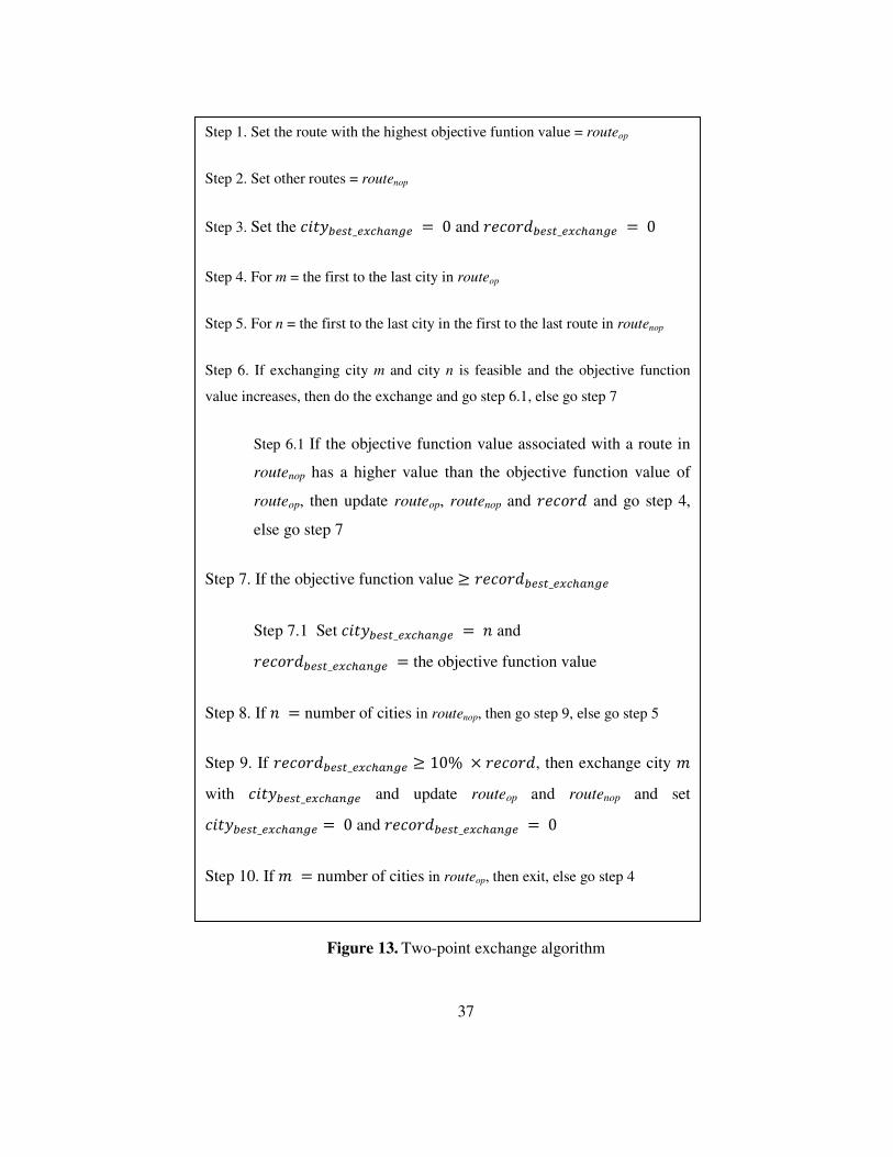
One point movement algorithm is given in Figure 14.

39

Figure 14. One point movement algorithm

Step 1. Set the �� Y��d_>��>�8d � 0 and '��!';Y��d_>��>�8d � 0

Step 2. For m = the first to the last city in ellipse or circle (say city ) is in route {)

Step 3. For n = the first to the last city in the first to the last route (route �) in both

routeop and routenop �{ a ��

Step 4. If inserting city m in front of city n is feasible and the objective function value

increases, then make the movement and go step 4.1, else go step 5

Step 4.1 If the objective function value associated with a route in routenop

has a higher value than the objective function value of routeop, then

update routeop, routenop and '��!'; and go step 2, else go step 5

Step 5. If the objective function value 5 '��!';Y��d_>��>�8d

Step 5.1 Set �� Y��d_>��>�8d � � and

'��!';Y��d_>��>�8d � the objective function value

Step 6. If � � number of cities in ellipse or circle - 1, then go step 7, else go step 3

Step 7. If '��!';Y��d_>��>�8d 5 10% j '��!';, then insert city ) in front

of �� Y��d_>��>�8d and update routeop and routenop and set �� Y��d_>��>�8d � 0 and '��!';Y��d_>��>�8d � 0

Step 8. If ) � number of cities in ellipse or circle, then exit, else go step 2

40

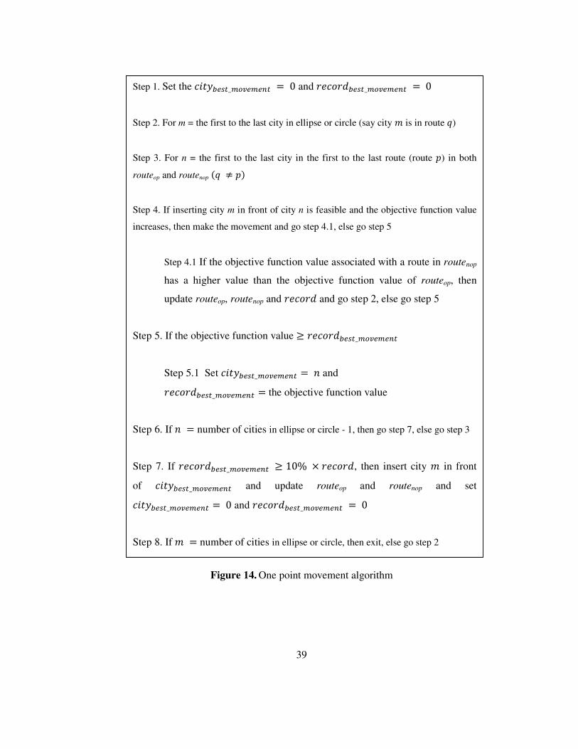
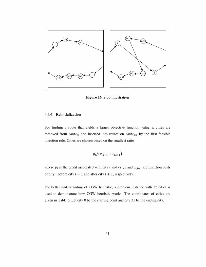
4.4.5 2 - Opt

For a given route with � cities, if ;�� , � cB� T ;I��, ��cBJ 5 ;I� , ��J T ;I� cB, ��cBJ, then the sequence of cities are changed to improve the route cost

as in Figure 16. In 2-opt algorithm, sequence of cities are changed based on maxM;�� , � cB� T ;I��, ��cBJ & ;I� , ��J T ;I� cB, ��cBJQ for � � 1,… , �. 2-

opt algorithm is given in Figure 15.

Figure 15. 2-opt algorithm

Step 1. Set the �� Sb��d � 0 , �� ) � 0, �� 0

Step 2. For m = the first to the last city in route p

Step 3. For n = the first to the last city in route p, � a )

Step 4. Calculate ;��>, �>cB� T ;��8, �8cB� & ;��>, �8� T ;��>cB, �8cB�

Step 5. If ;��>, �>cB� T ;��8, �8cB� & ;��>, �8� T ;��>cB, �8cB� 5�� Sb��d , then set �� Sb��d � ;��>, �>cB� T ;��8, �8cB� & ;��>, �8� T ;��>cB, �8cB� and �� ) � ), ��

Step 5. If � = number of cities in p, then go step 6, else go step 3

Step 6. If ) = number of cities in p, then go step 7, else go step 2

Step 7. If �� Sb��d x 0, then change the sequence of cities in route by �� )

and �� , and return step 1, else exit

41

Figure 16. 2-opt illustration

4.4.6 Reinitialization

For finding a route that yields a larger objective function value, k cities are

removed from routeop and inserted into routes on routenop by the first feasible

insertion rule. Cities are chosen based on the smallest ratio

� I� , bB T � , cBJ⁄

where � is the profit associated with city � and � , bB and � , cB are insertion costs

of city � before city � & 1 and after city � T 1, respectively.

For better understanding of CGW heuristic, a problem instance with 32 cities is

used to demonstrate how CGW heuristic works. The coordinates of cities are

given in Table 6. Let city 0 be the starting point and city 31 be the ending city.

i

i+1 i+2

j j+1 j+2

j+3

i

i+1 i+2

j j+1 j+2

j+3

42

Table 6. Co-ordinates of cities

� �� '!7� �� 0 10.5 14.4 0

1 18 15.9 10

2 18.3 13.3 10

3 16.5 9.3 10

4 15.4 11 10

5 14.9 13.2 5

6 16.3 13.3 5

7 16.4 17.8 5

8 15 17.9 5

9 16.1 19.6 10

10 15.7 20.6 10

11 13.2 20.1 10

12 14.3 15.3 5

13 14 5.1 10

14 11.4 6.7 15

15 8.3 5 15

16 7.9 9.8 10

17 11.4 12 5

18 11.2 17.6 5

19 10.1 18.7 5

20 11.7 20.3 10

21 10.2 22.1 10

22 9.7 23.8 10

23 10.1 26.4 15

24 7.4 24 15

25 8.2 19.9 15

26 8.7 17.7 10

27 8.9 13.6 10

28 5.6 11.1 10

29 4.9 18.9 10

30 7.3 18.8 10

31 11.2 14.1 0

The illustration of cities is given in Figure 17.

43

Figure 17. Illustration of cities for the sample problem

TMAX is set as 50 and all the cities are within the ellipse. The next step is

calculating the sum of the distance between each city and starting city and the

distance between each city and ending city and ordering the cities based on their

total distances. In Table 7, the sorted distances and the corresponding cities are

given.

Table 7. Sorted cities from maximum distance to minimum distance

2� � � ;

2� � � ;

2� � � ; 23 24.36 1 14.68 8 11.07

24 20.69 9 15.01 30 11.55

13 19.36 29 15.10 16 10.70

15 19.20 7 13.19 5 8.37

22 19.25 11 12.63 19 9.05

10 16.00 20 12.24 12 7.23

2 15.02 4 11.18 26 8.14

3 15.03 25 12.49 18 6.78

14 15.16 28 12.26 17 4.67

21 15.77 6 11.07 27 4.14

0

5

10

15

20

25

30

0 5 10 15 20

y co

-ord

inat

e

x co-ordinate

Cities

Starting City

End City

44

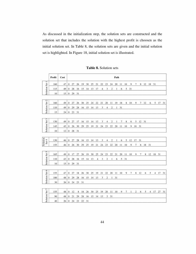
As discussed in the initialization step, the solution sets are constructed and the

solution set that includes the solution with the highest profit is choosen as the

initial solution set. In Table 8, the solution sets are given and the initial solution

set is highlighted. In Figure 18, initial solution set is illustrated.

Table 8. Solution sets

Profit Cost Path

S

olut

ion

Set

1

160 47 0 27 26 19 30 25 21 22 23 24 20 11 10 9 7 8 12 18 31

115 49 0 28 16 15 14 13 17 4 3 2 1 6 5 31

10 15 0 29 31

S

olut

ion

Set

2

160 49 0 27 26 30 25 24 22 21 20 11 19 18 8 10 9 7 12 6 5 17 31

110 49 0 29 28 16 15 14 13 3 4 2 1 31

15 24 0 23 31

S

olut

ion

Set

3

130 49 0 27 17 16 15 14 13 3 4 2 1 7 8 6 5 12 31

145 45 0 26 30 29 25 19 21 24 23 22 20 11 10 9 18 31

10 12 0 28 31

Sol

utio

n S

et 4

130 46 0 27 28 16 15 14 13 3 4 2 1 6 5 12 17 31

155 46 0 26 30 29 25 19 21 24 23 22 20 11 10 9 7 8 18 31

S

olut

ion

Set

5

165 49 0 17 27 26 19 30 25 24 23 22 21 20 11 10 9 7 8 12 18 31

110 43 0 28 16 15 14 13 4 3 2 1 6 5 31

10 15 0 29 31

S

olut

ion

Set

6

155 47 0 27 18 26 30 25 19 21 22 20 11 10 9 7 8 12 6 5 4 17 31

100 48 0 29 28 16 15 14 13 3 2 1 31

30 26 0 24 23 31

S

olut

ion

Set

7

155 48 0 12 8 18 26 30 25 19 20 11 10 9 7 1 2 6 5 4 17 27 31

90 48 0 21 29 28 16 15 14 13 3 31

40 26 0 24 23 22 31

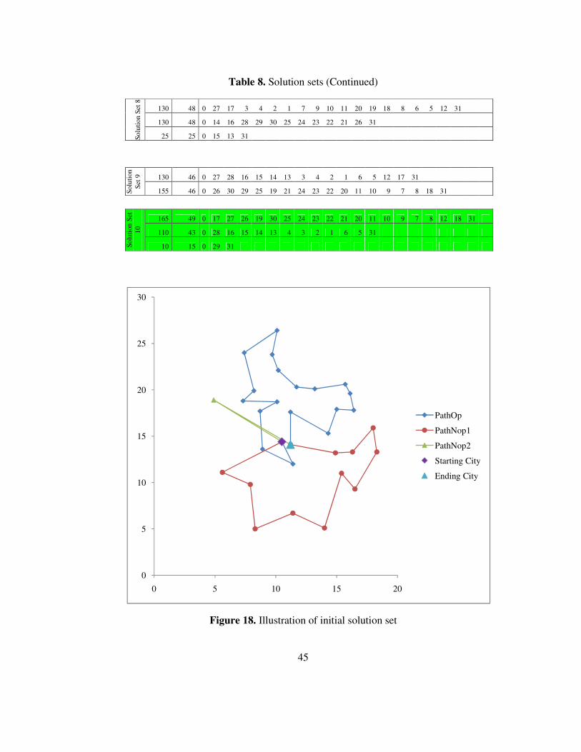
45

Table 8. Solution sets (Continued)

Sol

utio

n S

et 8

130 48 0 27 17 3 4 2 1 7 9 10 11 20 19 18 8 6 5 12 31

130 48 0 14 16 28 29 30 25 24 23 22 21 26 31

25 25 0 15 13 31

Sol

utio

n S

et 9

130 46 0 27 28 16 15 14 13 3 4 2 1 6 5 12 17 31

155 46 0 26 30 29 25 19 21 24 23 22 20 11 10 9 7 8 18 31

Sol

utio

n S

et

10

165 49 0 17 27 26 19 30 25 24 23 22 21 20 11 10 9 7 8 12 18 31

110 43 0 28 16 15 14 13 4 3 2 1 6 5 31

10 15 0 29 31

Figure 18. Illustration of initial solution set

0

5

10

15

20

25

30

0 5 10 15 20

PathOp

PathNop1

PathNop2

Starting City

Ending City

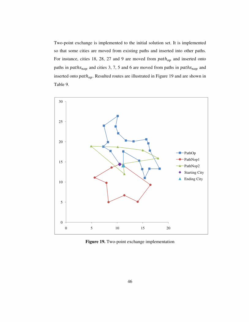
46

Two-point exchange is implemented to the initial solution set. It is implemented

so that some cities are moved from existing paths and inserted into other paths.

For instance, cities 18, 28, 27 and 9 are moved from �� P�� and inserted onto

paths in �� P�8�� and cities 3, 7, 5 and 6 are moved from paths in �� P�8�� and

inserted onto �� P��. Resulted routes are illustrated in Figure 19 and are shown in

Table 9.

Figure 19. Two-point exchange implementation

0

5

10

15

20

25

30

0 5 10 15 20

PathOp

PathNop1

PathNop2

Starting City

Ending City

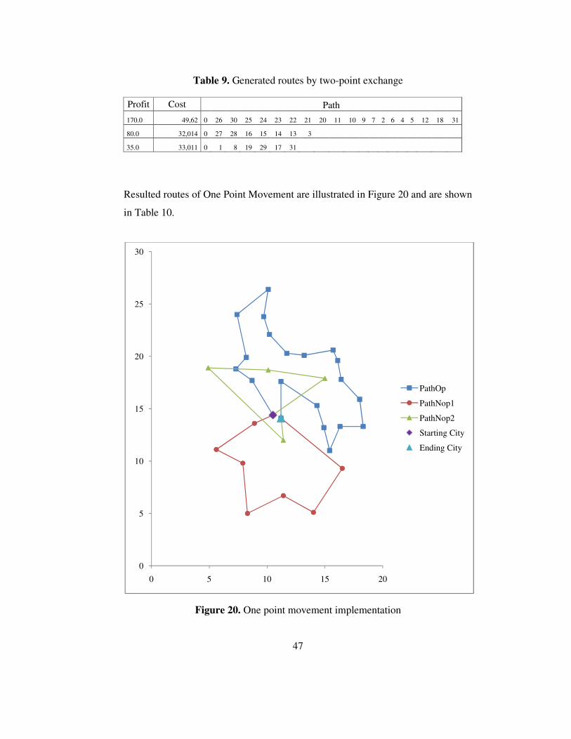
47

Table 9. Generated routes by two-point exchange

Profit Cost Path

170.0 49,62 0 26 30 25 24 23 22 21 20 11 10 9 7 2 6 4 5 12 18 31

80.0 32,014 0 27 28 16 15 14 13 3

35.0 33,011 0 1 8 19 29 17 31

Resulted routes of One Point Movement are illustrated in Figure 20 and are shown

in Table 10.

Figure 20. One point movement implementation

0

5

10

15

20

25

30

0 5 10 15 20

PathOp

PathNop1

PathNop2

Starting City

Ending City

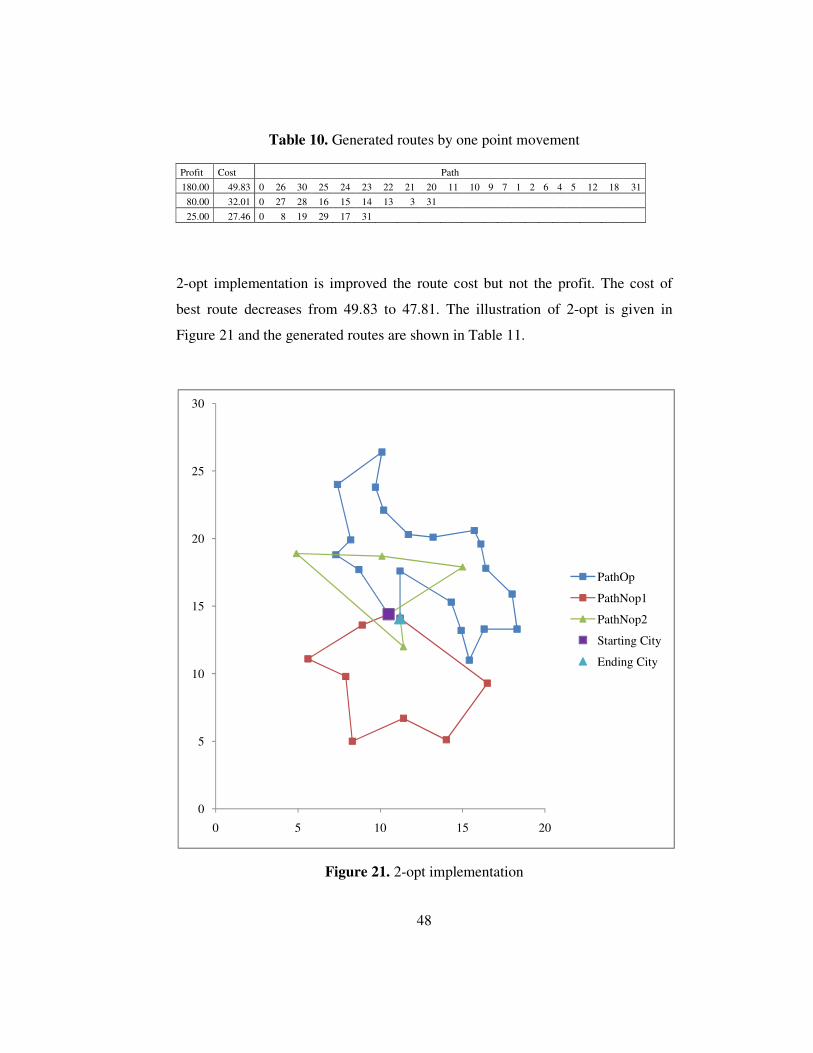
48

Table 10. Generated routes by one point movement

Profit Cost Path

180.00 49.83 0 26 30 25 24 23 22 21 20 11 10 9 7 1 2 6 4 5 12 18 31

80.00 32.01 0 27 28 16 15 14 13 3 31

25.00 27.46 0 8 19 29 17 31

2-opt implementation is improved the route cost but not the profit. The cost of

best route decreases from 49.83 to 47.81. The illustration of 2-opt is given in

Figure 21 and the generated routes are shown in Table 11.

Figure 21. 2-opt implementation

0

5

10

15

20

25

30

0 5 10 15 20

PathOp

PathNop1

PathNop2

Starting City

Ending City

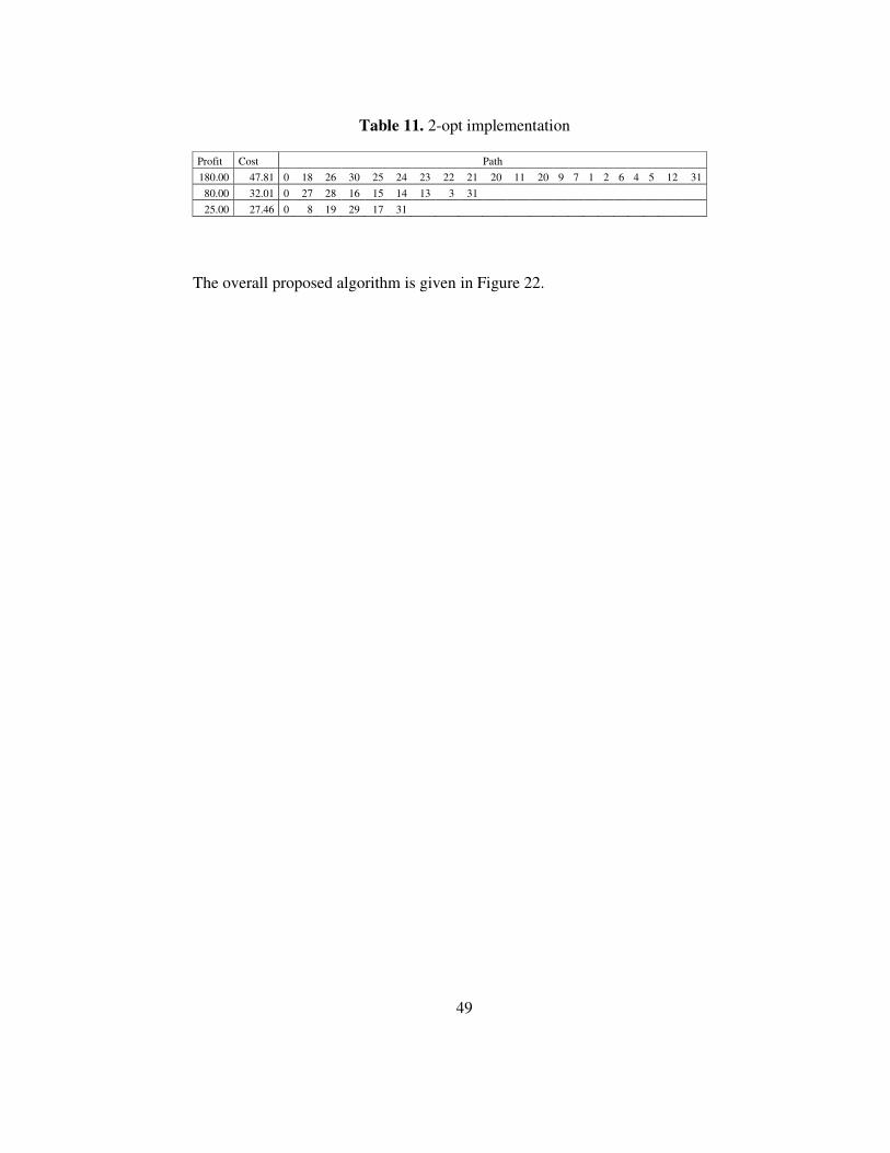
49

Table 11. 2-opt implementation

Profit Cost Path

180.00 47.81 0 18 26 30 25 24 23 22 21 20 11 20 9 7 1 2 6 4 5 12 31

80.00 32.01 0 27 28 16 15 14 13 3 31

25.00 27.46 0 8 19 29 17 31

The overall proposed algorithm is given in Figure 22.

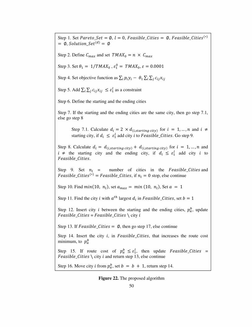
50

Figure 22. The proposed algorithm

Step 1. Set ��'� !_� � f, ( � 0, y��(�_2� �� f, y��(�_2� �� f, !(� �!�_� �� f

Step 2. Define 2>Wi and set ��: � � j 2>Wi

Step 3. Set hB � 1 ��:⁄ , �B: � ��:, � � 0.0001

Step 4. Set objective function as ∑ � � & hB ∑ ∑ � ��

Step 5. Add ∑ ∑ � �� 1 �Bg as a constraint

Step 6. Define the starting and the ending cities

Step 7. If the starting and the ending cities are the same city, then go step 7.1, else go step 8

Step 7.1. Calculate ; � 2 j ;� ,�dW�d 8� z d�� for � � 1, … , � and � a

starting city, if ; 1 �Bg add city � to y��(�_2� ��. Go step 9.

Step 8. Calculate ; � ;� ,�dW�d 8� z d�� T ;� ,�dW�d 8� z d�� for � � 1, … , � and � a the starting city and the ending city, if ; 1 �Bg add city � to y��(�_2� ��.

Step 9. Set �g = number of cities in the y��(�_2� �� and y��(�_2� �� y��(�_2� ��, if �g � 0 stop, else continue

Step 10. Find )��10, �g�, set �>Wi � )�� 10, �g�, Set � � 1

Step 11. Find the city � with �de largest ; in y��(�_2� ��, set � � 1

Step 12. Insert city � between the starting and the ending cities, �WY, update y��(�_2� �� = y��(�_2� �� | city � Step 13. If y��(�_2� �� f, then go step 17, else continue

Step 14. Insert the city �, in y��(�_2� ��, that increases the route cost minimum, to �WY

Step 15. If route cost of �WY 1 �Bg , then update y��(�_2� �� = y��(�_2� �� | city � and return step 13, else continue

Step 16. Move city � from �WY, set � � � T 1, return step 14.

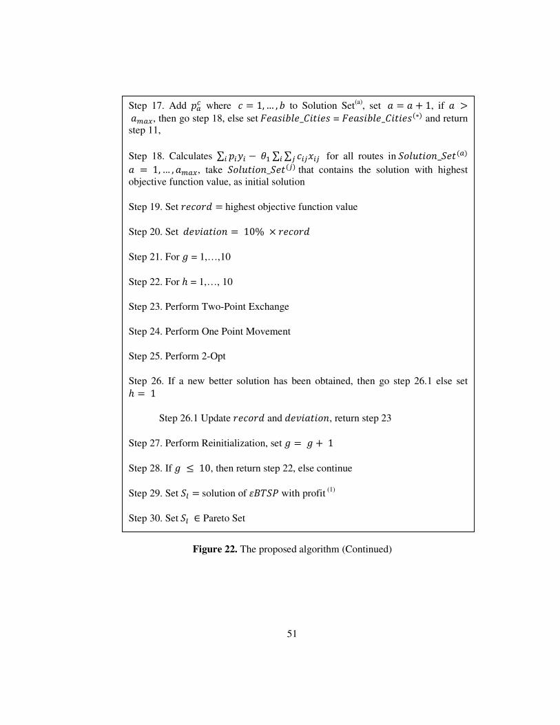
51

Figure 22. The proposed algorithm (Continued)

Step 17. Add �Wz where � � 1,… , � to Solution Set(a), set � � � T 1, if � x �>Wi, then go step 18, else set y��(�_2� �� = y��(�_2� �� and return step 11,

Step 18. Calculates ∑ � � & hB ∑ ∑ � �� for all routes in !(� �!�_� �W� � � 1, … , �>Wi, take !(� �!�_� �� that contains the solution with highest objective function value, as initial solution

Step 19. Set '��!'; � highest objective function value

Step 20. Set ;�� !� � 10% j '��!';

Step 21. For N = 1,…,10

Step 22. For P = 1,…, 10

Step 23. Perform Two-Point Exchange

Step 24. Perform One Point Movement

Step 25. Perform 2-Opt

Step 26. If a new better solution has been obtained, then go step 26.1 else set P � 1 Step 26.1 Update '��!'; and ;�� !�, return step 23

Step 27. Perform Reinitialization, set N � N T 1

Step 28. If N 1 10, then return step 22, else continue

Step 29. Set g � solution of �� with profit (1)


( � ( T 1

52

CHAPTER 5

SOLUTION SET ANALYSIS

Multiobjective optimization can be regarded as a systematic sensitivity analysis of

the most important value judgments. An essential feature in the multiobjective

approach is the generation of several good alternatives (i.e. Pareto optimal

solutions) and the comparison of them with each other. If there is only one

alternative, like an optimal solution of a scalar problem, then the only decision is

if that solution is acceptable or not. A real decision making becomes possible only

if there are several alternatives which should be judged in order to pick up the best

one. One approach to find the best solution, is finding the set of good solutions by

calculating distances of Pareto optimal solutions to a given infeasible alternative.

The distance formulation includes the parameter � � 1,… ,∞. Base on the chosen

value of parameter �, the distance value changes. The solutions which have the

minimum distance for at least one of � value for � � 1, … ,∞ constructs the set of

effective solutions. Then trade-off concept can be applied in choosing the best

solution among good solutions. In section 5.1, some definitions used in this

chapter are described, and then experimental computations and the procedure to

find the good solutions are explained and some illustrations are shown in section

5.2. Finally, trade-off concept is described in section 5.3.

5.1 Some Definitions

An ideal point (ideal solution) is generally an infeasible alternative consisting of

the best value for each objective function. Each objective function is optimized

subject to the given constraints, separately in order to obtain ideal point.

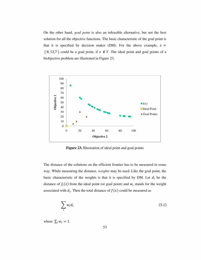
53

On the other hand, goal point is also an infeasible alternative, but not the best

solution for all the objective functions. The basic characteristic of the goal point is

that it is specified by decision maker (DM). For the above example, � � , 8, 12,7 . could be a goal point, if � � R. The ideal point and goal points of a

biobjective problem are illustrated in Figure 23.

Figure 23. Illustration of ideal point and goal points

The distance of the solutions on the efficient frontier has to be measured in some

way. While measuring the distance, weights may be used. Like the goal point, the

basic characteristic of the weights is that it is specified by DM. Let ; be the

distance of 7 �� from the ideal point (or goal point) and � stands for the weight

associated with ; . Then the total distance of 7�� could be measured as

�� ; �5.1�

where ∑ � � 1 .

0

10

20

30

40

50

60

70

80

90

100

0 20 40 60 80 100

Ob

ject

ive

1

Objective 2

f(x)

Ideal Point

Goal Points

54

5.2 Distance Formulation

Let � and � + =>, � @ � + = and � @ � + = for � � 1,… ,). The distance

between � and � could be described as

;� � ��|�D & �D|�>D9B �B/� �5.2�

Where � 5 1 which means that � may take any value from 1 to T∞.

For � � 2, Equation (5.2) calculates Euclidean distance between two points. For a

given points x and y + =S, Equation (5.2) becomes

;S � ��B & �B�S T ��S & �S�S�

For � � 1 and T∞, Equation (5.2) calculates Manhattan and Tchebycheff

distances between two points, respectively. The distances ;B and ;� represent

bounds on the distance between any two points

;B 5 ;� 5 ;� �5.3�

For the weighted case, Equation (5.2) is modified as

;� � ��D|�D & �D|�>D9B �B/� �5.4�

where ∑ � � 1 .

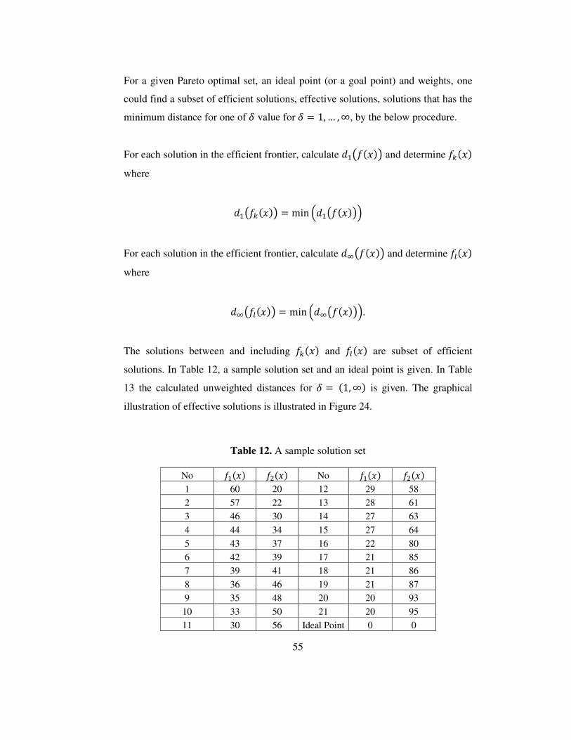
55

For a given Pareto optimal set, an ideal point (or a goal point) and weights, one

could find a subset of efficient solutions, effective solutions, solutions that has the

minimum distance for one of � value for � � 1,… ,∞, by the below procedure.

For each solution in the efficient frontier, calculate ;BI7��J and determine 7D��

where

;BI7D��J � min �;BI7��J�

For each solution in the efficient frontier, calculate ;�I7��J and determine 7g��

where

;�I7g��J � min �;�I7��J�.

The solutions between and including 7D�� and 7g�� are subset of efficient

solutions. In Table 12, a sample solution set and an ideal point is given. In Table

13 the calculated unweighted distances for � � �1,∞� is given. The graphical

illustration of effective solutions is illustrated in Figure 24.

Table 12. A sample solution set

No 7B�� 7S�� No 7B�� 7S��

1 60 20 12 29 58

2 57 22 13 28 61

3 46 30 14 27 63

4 44 34 15 27 64

5 43 37 16 22 80

6 42 39 17 21 85

7 39 41 18 21 86

8 36 46 19 21 87

9 35 48 20 20 93

10 33 50 21 20 95

11 30 56 Ideal Point 0 0

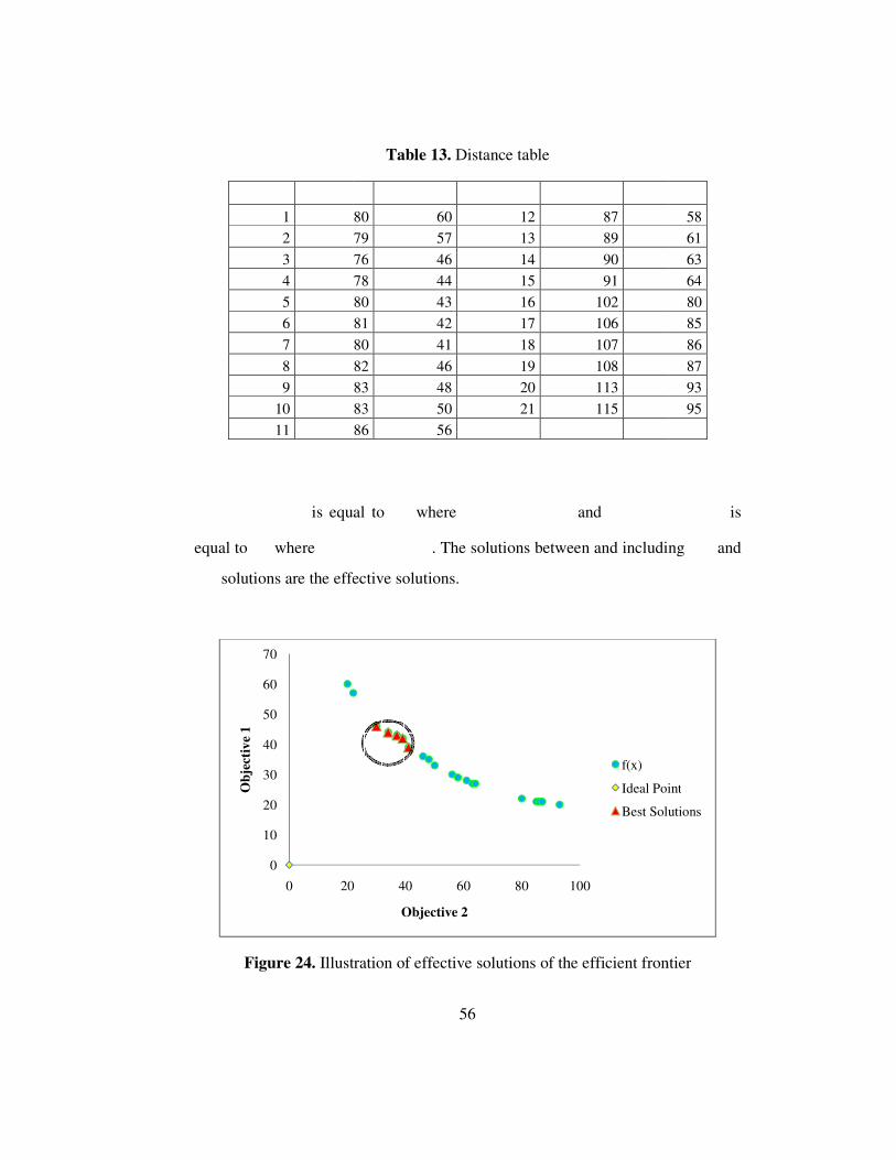
1

2

3

4

5

6

7

8

9

10

11

is equal to

equal to where

solutions are the effective solutions.

Figure 24. Illustration of effective solutions of the efficient frontier

0

10

20

30

40

50

60

70

0 20

Ob

ject

ive

1

56

Table 13. Distance table

80 60 12 87

79 57 13 89

76 46 14 90

78 44 15 91

80 43 16 102

81 42 17 106

80 41 18 107

82 46 19 108

83 48 20 113

83 50 21 115

86 56

is equal to where and

. The solutions between and including

solutions are the effective solutions.

Illustration of effective solutions of the efficient frontier

20 40 60 80 100

Objective 2

f(x)

Ideal Point

Best Solutions

58

61

63

64

80

85

86

87

93

95

is

. The solutions between and including and

Illustration of effective solutions of the efficient frontier

Ideal Point

Best Solutions

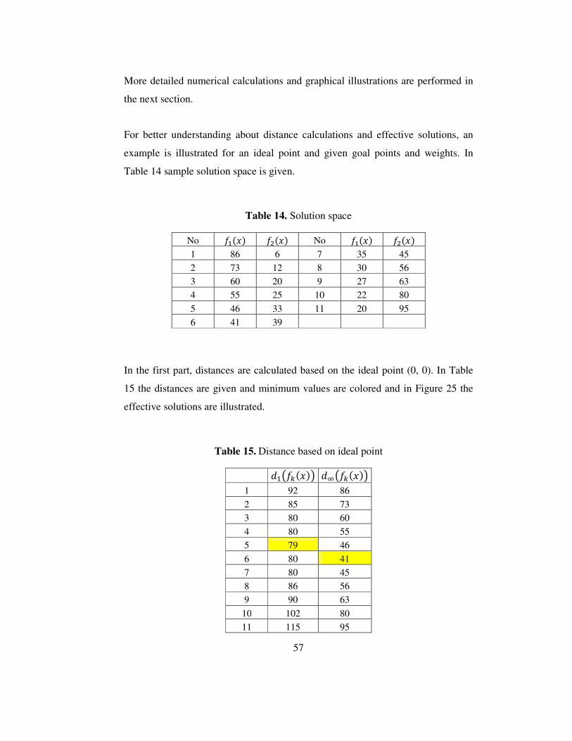
57

More detailed numerical calculations and graphical illustrations are performed in

the next section.

For better understanding about distance calculations and effective solutions, an

example is illustrated for an ideal point and given goal points and weights. In

Table 14 sample solution space is given.

Table 14. Solution space

No 7B�� 7S�� No 7B�� 7S��

1 86 6 7 35 45

2 73 12 8 30 56

3 60 20 9 27 63

4 55 25 10 22 80

5 46 33 11 20 95

6 41 39

In the first part, distances are calculated based on the ideal point (0, 0). In Table

15 the distances are given and minimum values are colored and in Figure 25 the

effective solutions are illustrated.

Table 15. Distance based on ideal point

;BI7D��J ;�I7D��J

1 92 86

2 85 73

3 80 60

4 80 55

5 79 46

6 80 41

7 80 45

8 86 56

9 90 63

10 102 80

11 115 95

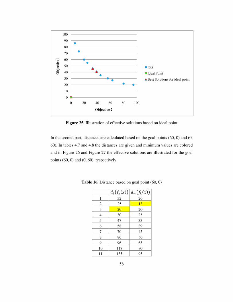
58

Figure 25. Illustration of effective solutions based on ideal point

In the second part, distances are calculated based on the goal points (60, 0) and (0,

60). In tables 4.7 and 4.8 the distances are given and minimum values are colored

and in Figure 26 and Figure 27 the effective solutions are illustrated for the goal

points (60, 0) and (0, 60), respectively.

Table 16. Distance based on goal point (60, 0)


1 32 26

2 25 13

3 20 20

4 30 25

5 47 33

6 58 39

7 70 45

8 86 56

9 96 63

10 118 80

11 135 95

0

10

20

30

40

50

60

70

80

90

100

0 20 40 60 80 100

Ob

ject

ive

1

Objective 2

f(x)

Ideal Point

Best Solutions for ideal point

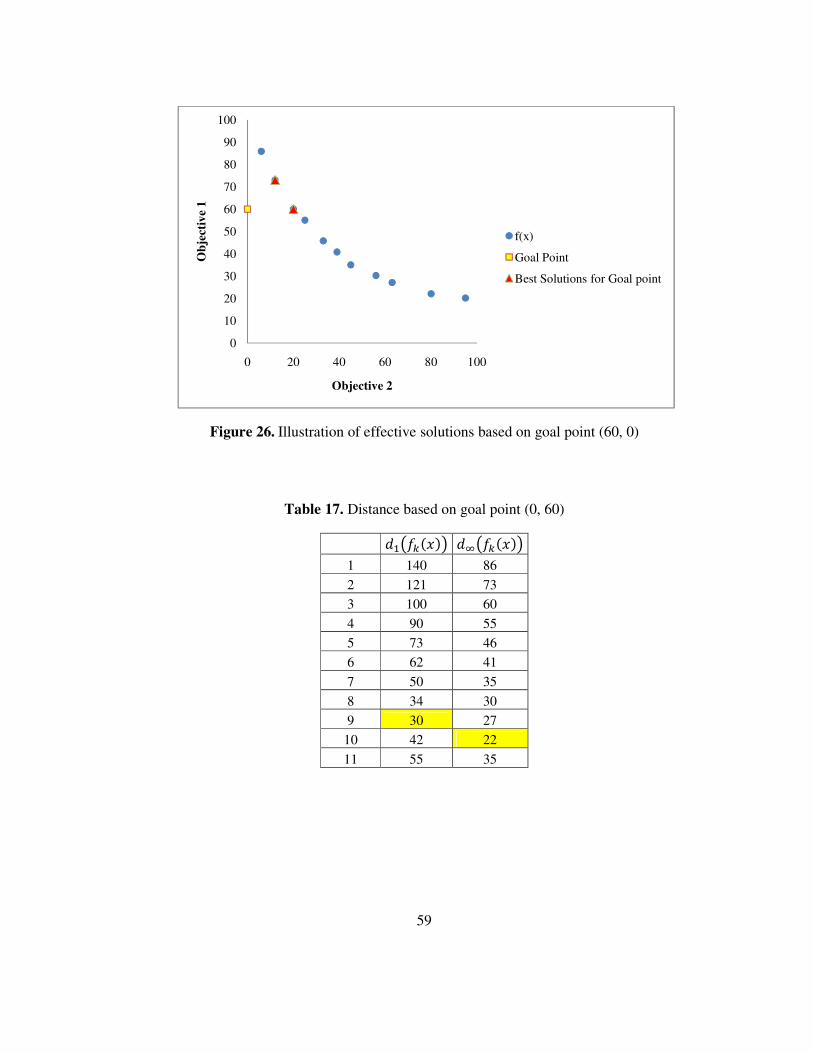
59

Figure 26. Illustration of effective solutions based on goal point (60, 0)

Table 17. Distance based on goal point (0, 60)


1 140 86

2 121 73

3 100 60

4 90 55

5 73 46

6 62 41

7 50 35

8 34 30

9 30 27

10 42 22

11 55 35

0

10

20

30

40

50

60

70

80

90

100

0 20 40 60 80 100

Ob

ject

ive

1

Objective 2

f(x)

Goal Point

Best Solutions for Goal point

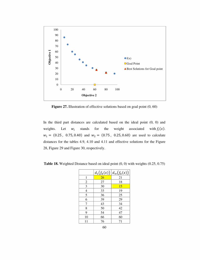
60

Figure 27. Illustration of effective solutions based on goal point (0, 60)

In the third part distances are calculated based on the ideal point (0, 0) and

weights. Let � stands for the weight associated with 7 ��. �B � �0.25 , 0.75, 0.40� and �S � �0.75 , 0.25, 0.60� are used to calculate

distances for the tables 4.9, 4.10 and 4.11 and effective solutions for the Figure

28, Figure 29 and Figure 30, respectively.

Table 18. Weighted Distance based on ideal point (0, 0) with weights (0.25, 0.75)


1 26 21 2 27 18 3 30 15 4 33 19 5 36 25 6 39 29 7 43 34 8 50 42 9 54 47

10 66 60 11 76 71

0

10

20

30

40

50

60

70

80

90

100

0 20 40 60 80 100

Ob

ject

ive

1

Objective 2

f(x)

Goal Point

Best Solutions for Goal point

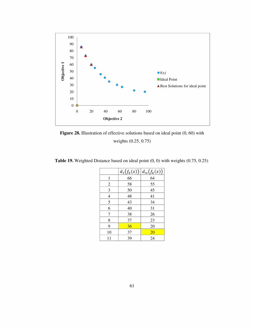
61

Figure 28. Illustration of effective solutions based on ideal point (0, 60) with

weights (0.25, 0.75)



1 66 64

2 58 55

3 50 45

4 48 41

5 43 34

6 40 31

7 38 26

8 37 23

9 36 20

10 37 20

11 39 24

0

10

20

30

40

50

60

70

80

90

100

0 20 40 60 80 100

Ob

ject

ive

1

Objective 2

f(x)

Ideal Point


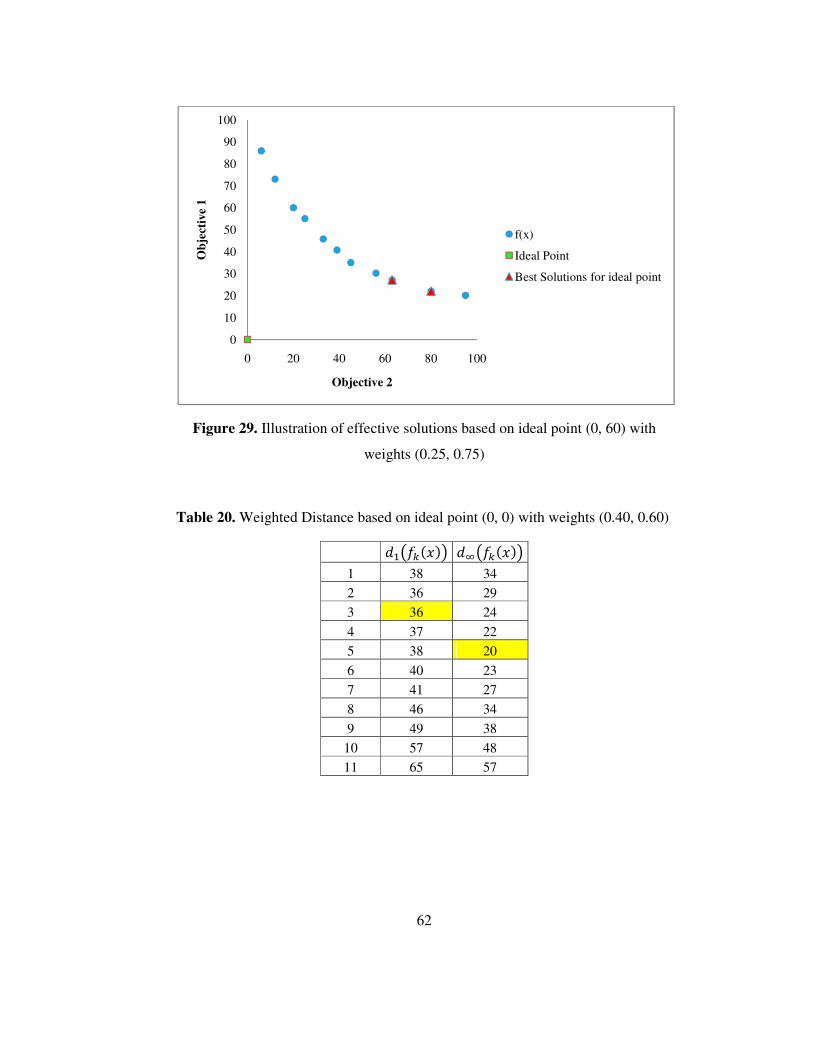
62

Figure 29. Illustration of effective solutions based on ideal point (0, 60) with

weights (0.25, 0.75)



1 38 34

2 36 29

3 36 24

4 37 22

5 38 20

6 40 23

7 41 27

8 46 34

9 49 38

10 57 48

11 65 57

0

10

20

30

40

50

60

70

80

90

100

0 20 40 60 80 100

Ob

ject

ive

1

Objective 2

f(x)

Ideal Point


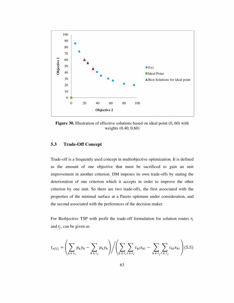
63

Figure 30. Illustration of effective solutions based on ideal point (0, 60) with weights (0.40, 0.60)

5.3 Trade-Off Concept

Trade-off is a frequently used concept in multiobjective optimization. It is defined

as the amount of one objective that must be sacrificed to gain an unit

improvement in another criterion. DM imposes its own trade-offs by stating the

deterioration of one criterion which it accepts in order to improve the other

criterion by one unit. So there are two trade-offs, the first associated with the

properties of the minimal surface at a Pareto optimum under consideration, and

the second associated with the preferences of the decision maker.

For Biobjective TSP with profit the trade-off formulation for solution routes ' and '�, can be given as

�� D�DD + ��& � �D�DD + �

¡ � � � �Dg�Dg g + ��D + ��& � � �Dg�Dg g + � D + �

¡¢ �5.5�

0

10

20

30

40

50

60

70

80

90

100

0 20 40 60 80 100

Ob

ject

ive

1

Objective 2

f(x)

Ideal Point


64

where is the profit associated with city k and is the cost associated with the

route between city and city . Equation (1) means that one unit of cost objective

can be sacrificed to gain unit improvement in profit objective by choosing

instead of .

Let , and ,

for a given solution routes and . Then

One unit of cost objective can be sacrificed to gain unit improvement in profit

objective by choosing instead of . If the preference of DM is choosing

instead of which means the trade off is acceptable for DM, is set as candidate

best solution. This process continues until there is no trade-off, which DM

accepted, for the candidate best solution or another termination condition is

guaranteed. Then candidate best solution is set as best solution.

Figure 31. Trade off diagram for the sample solution set in Table 14

0

0,5

1

1,5

2

2,5

0

0,2

0,4

0,6

0,8

1

1,2

0 2 4 6 8 10 12

Objective 1

Objective 2

Trade off

65

In Figure 31, the trade off diagram for the sample solution set in Table 14 is

shown. The trade off values for solution � is the trade of value for solution � & 1

and solution �. Because of that the trade off value for solution 1 is represented as

0. Base on the information given by trade off diagram DM can easily see that the

trade off between solution 1 and solution 2 is high, one unit increase in objective 2

causes two unit decrease in objective 1. For the high level picture DM can prefer

solution 2 or he can check other solutions depending on the trade off level he can

accept.

The marked area is the effective solutions set for the ideal point (0,0). Moving

from solution 5 to solution 6 causes 0.83 unit decrease in objective 1 for 1 unit

increase in objective 2. If DM can not accept the trade offs smaller than 1 unit

decrease in objective 1 for 1 unit increase in objective 2 he would choose solution

5. If it is acceptable he will choose solution 6.

66

CHAPTER 6

COMPUTATIONAL RESULTS

The performance of the �-constrained method is evaluated by applying the method

to 5 problem sets taken from the literature and comparing the solutions with the

results in the literature. Also, the method is applied to 9 problem sets taken from

the literature and the solutions are compared not fully by partially with the

published results, since these problem sets are solved partially.

In section 6.1, the problem sets are given. In section 6.2, the performance of the �-

constrained method is discussed. Finally, the solutions of the problem sets out of

problem sets used for performance evaluation are given in section 6.3.

6.1 Problem Sets

We considered 2 different classes of test problems. The first problem class

includes 5 instances from the OP literature and Biobjective TSP with Profit

literature. Problems OP21, OP32, and OP33 are OP instances introduced by

Tsiligirides (1984). Problem OP32-1- instance is introduced by Chao et al. (1998).

In the literature OP problem sets are solved with fixed parameters for the right

hand side of route cost constraint. Problem K25 instance is introduced by Keller

and Goodchild (1986). Keller and Goodchild (1986) use only K25 problem set for

their algorithm.

The second problem class includes 9 instances from Vehicle Routing Problem

(VRP) literature. Problems ATT48, EIL30, EIL33, EIL51, EIL76, and EIL101 are

VRP instances taken from the Traveling Salesman Problem Library TSPLIB of

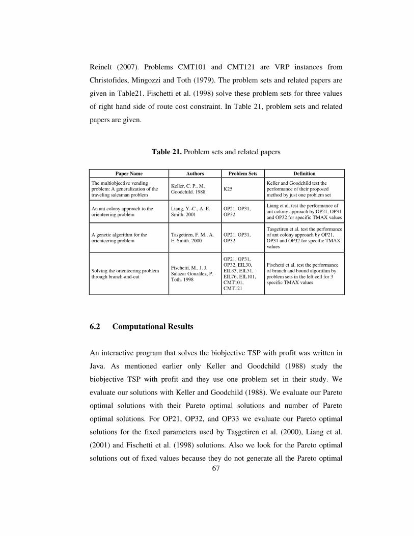
67

Reinelt (2007). Problems CMT101 and CMT121 are VRP instances from

Christofides, Mingozzi and Toth (1979). The problem sets and related papers are

given in Table21. Fischetti et al. (1998) solve these problem sets for three values

of right hand side of route cost constraint. In Table 21, problem sets and related

papers are given.

Table 21. Problem sets and related papers

Paper Name Authors Problem Sets Definition

The multiobjective vending problem: A generalization of the traveling salesman problem

Keller, C. P., M. Goodchild. 1988

K25 Keller and Goodchild test the performance of their proposed method by just one problem set

An ant colony approach to the orienteering problem

Liang, Y.-C., A. E. Smith. 2001

OP21, OP31, OP32

Liang et al. test the performance of ant colony approach by OP21, OP31 and OP32 for specific TMAX values

A genetic algorithm for the orienteering problem

Tasgetiren, F. M., A. E. Smith. 2000

OP21, OP31, OP32

Tasgetiren et al. test the performance of ant colony approach by OP21, OP31 and OP32 for specific TMAX values

Solving the orienteering problem through branch-and-cut

Fischetti, M., J. J. Salazar González, P. Toth. 1998

OP21, OP31, OP32, EIL30, EIL33, EIL51, EIL76, EIL101, CMT101, CMT121

Fischetti et al. test the performance of branch and bound algorithm by problem sets in the left cell for 3 specific TMAX values

6.2 Computational Results

An interactive program that solves the biobjective TSP with profit was written in

Java. As mentioned earlier only Keller and Goodchild (1988) study the

biobjective TSP with profit and they use one problem set in their study. We

evaluate our solutions with Keller and Goodchild (1988). We evaluate our Pareto

optimal solutions with their Pareto optimal solutions and number of Pareto

optimal solutions. For OP21, OP32, and OP33 we evaluate our Pareto optimal

solutions for the fixed parameters used by Taşgetiren et al. (2000), Liang et al.

(2001) and Fischetti et al. (1998) solutions. Also we look for the Pareto optimal

solutions out of fixed values because they do not generate all the Pareto optimal

68

solutions. We also look for the Pareto optimal solutions we found where they have

same profits as the solutions Fischetti et al. found but the route costs are less than

their solutions. By this we can show that we can found better solutions for the

fixed values. The other computational analyze is trade off relations. By trade-off

relations we mean showing that for a small increase in the route cost if we can

generate solutions with higher profits then their solutions.

On the other hand, K25, OP21, OP32, OP33, and OP32-1- problem sets are also

used to demonstrate and evaluate the performance of the �-constraint method. The

results show that �-constraint method found all solutions for specific TMAX

values published in the literature.

Figure 32. Pareto optimal solutions for K25 problem set

In literature, the only true attempt for solving the biobjective TSP with profit was

Keller and Goodchild (1988). Keller and Goodchild (1988) test the performance

0

2000

4000

6000

8000

10000

12000

14000

0 500 1000 1500 2000 2500 3000 3500 4000

Pro

fit

Cost

69

of their proposed method by just one problem set that includes 25 cities located in

West Germany. Bonn was used as the depot and terminal node. The populations

of cities were treated as profit associated with each city.

The number of solutions obtained by Keller was 27 which is less than 71 solutions

that we obtained. 18 solutions obtained by our method are also obtained by Keller.

Keller could not obtain 44 solutions that we obtain. 9 solutions dominated 9

Keller solutions. In Figure 31, the Pareto optimal solutions are given for K25. In

Figure 32, the trade-off is shown for K25. In this figure and in all trade-off

figures, route profits and costs are scalarized between 0 – 1 and shown by left

vertical axis. Also, trade-offs are calculated for each solution. From left to right,

trade-off values means decrease in profit for one unit decrease in cost. It is reverse

from right to left. The values for trade-offs are shown by right vertical axis.

Figure 33. Scalarization of profit and cost, and trade-off for K25 problem set

0

20

40

60

80

100

120

0

0,2

0,4

0,6

0,8

1

1,2

1 6 10 14 18 22 26 30 34 38 42 46 50 54 58 62 66 70

un

it P

rofi

t ga

ined

/on

e u

nit

cos

t in

curr

ed

Sca

lari

zed

Val

ue

Solution No

Profit

Cost

Trade-off

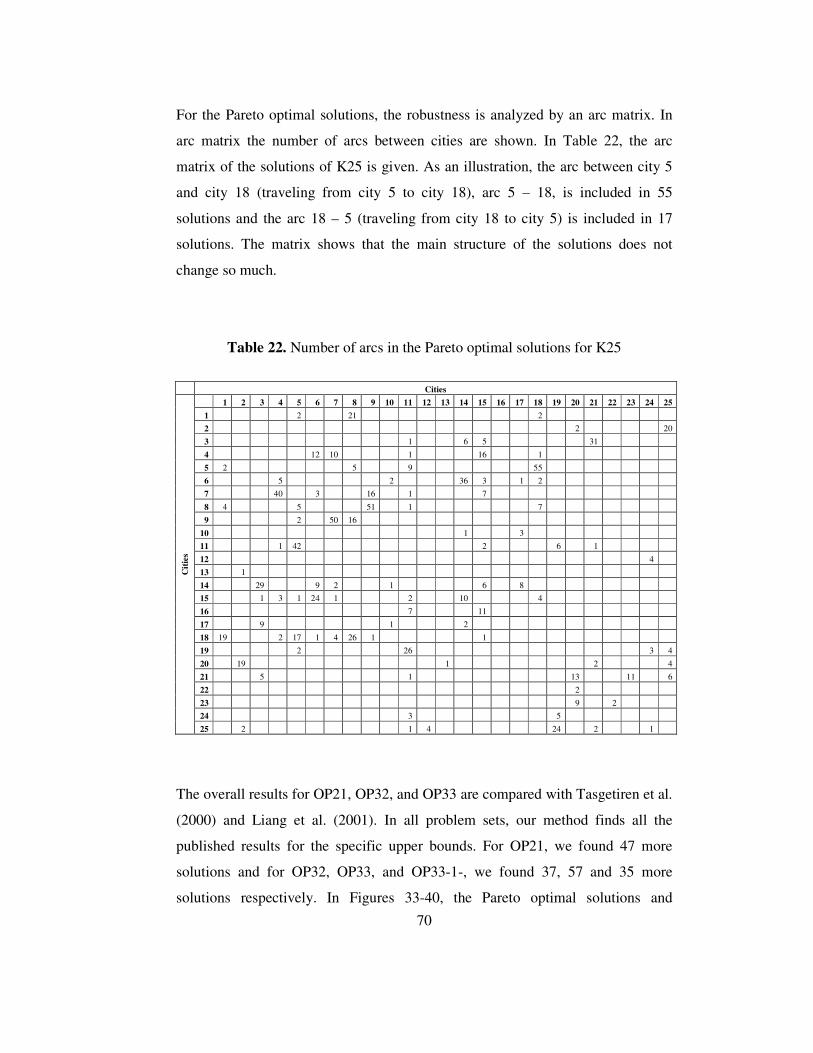
70

For the Pareto optimal solutions, the robustness is analyzed by an arc matrix. In

arc matrix the number of arcs between cities are shown. In Table 22, the arc

matrix of the solutions of K25 is given. As an illustration, the arc between city 5

and city 18 (traveling from city 5 to city 18), arc 5 – 18, is included in 55

solutions and the arc 18 – 5 (traveling from city 18 to city 5) is included in 17

solutions. The matrix shows that the main structure of the solutions does not

change so much.

Table 22. Number of arcs in the Pareto optimal solutions for K25

Cities

Cit

ies

1 2 3 4 5 6 7 8 9 10 11 12 13 14 15 16 17 18 19 20 21 22 23 24 25

1 2 21 2

2 2 20

3 1 6 5 31

4 12 10 1 16 1

5 2 5 9 55

6 5 2 36 3 1 2

7 40 3 16 1 7

8 4 5 51 1 7

9 2 50 16

10 1 3

11 1 42 2 6 1

12 4

13 1

14 29 9 2 1 6 8

15 1 3 1 24 1 2 10 4

16 7 11

17 9 1 2

18 19 2 17 1 4 26 1 1

19 2 26 3 4

20 19 1 2 4

21 5 1 13 11 6

22 2

23 9 2

24 3 5

25 2 1 4 24 2 1

The overall results for OP21, OP32, and OP33 are compared with Tasgetiren et al.

(2000) and Liang et al. (2001). In all problem sets, our method finds all the

published results for the specific upper bounds. For OP21, we found 47 more

solutions and for OP32, OP33, and OP33-1-, we found 37, 57 and 35 more

solutions respectively. In Figures 33-40, the Pareto optimal solutions and

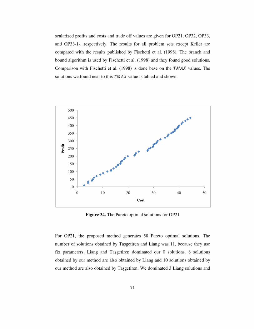
71

scalarized profits and costs and trade off values are given for OP21, OP32, OP33,

and OP33-1-, respectively. The results for all problem sets except Keller are

compared with the results published by Fischetti et al. (1998). The branch and

bound algorithm is used by Fischetti et al. (1998) and they found good solutions.

Comparison with Fischetti et al. (1998) is done base on the �� values. The

solutions we found near to this �� value is tabled and shown.

Figure 34. The Pareto optimal solutions for OP21

For OP21, the proposed method generates 58 Pareto optimal solutions. The

number of solutions obtained by Taşgetiren and Liang was 11, because they use

fix parameters. Liang and Taşgetiren dominated our 0 solutions. 8 solutions

obtained by our method are also obtained by Liang and 10 solutions obtained by

our method are also obtained by Taşgetiren. We dominated 3 Liang solutions and

0

50

100

150

200

250

300

350

400

450

500

0 10 20 30 40 50

Pro

fit

Cost

72

1 Taşgetiren solutions. Taşgetiren and Liang could not obtain 47 solutions that we

obtain.

Fischetti et al. (1998) uses 11.50, 22.99, and 34.49 for��. Based on these

TMAX values our solutions and neighborhood solutions are given in Table 23.

For route cost 34.49 the published result is better than the generated result but for

route cost 34.51 the generated solution has a profit value of 320 which is higher

than 315, which means for 0.51 unit increase in route cost we gain 5 unit of profit.

For route cost 22.99 the generated solution is better than the published result.

Also, for 23.06 the generated solution has a profit value of 220, which means for

0.06 unit increase in route cost we gain 15 unit of profit. For route cost 11.50 the

generated solution is same with the published result but our solution has a lower

route cost. Also for 11.81 the generated solution has a profit value of 100. In

Table 24, the arc matrix of the solutions of OP21 is given. As it can be seen that

some arcs are included in most of the solutions and most of the arcs are not

included in the solutions. For instance, arcs 9 – 10, 10 – 11, and 11 – 13 are

included in most of the solutions and arcs 1 – 4, 8 – 2, and 11 – 8 are not included

in any solutions. The main structure of the solutions does not change so much.

Table 23. Published solutions and neighborhood solutions for OP21 for the given �� values

Profit Cost Profit Cost Profit Cost

Fischetti et al. Solutions 315 34.49 205 22.99 90 11.50

Generated Solutions

340 35.86227 230 24.128345 105 13.231623

330 35.446358 220 23.063688 100 11.818177

320 34.514474 210 22.647777 90 10.103147

310 32.690083 205 22.513478 80 9.0272882

300 31.625426 200 19.879525 70 7.5491731

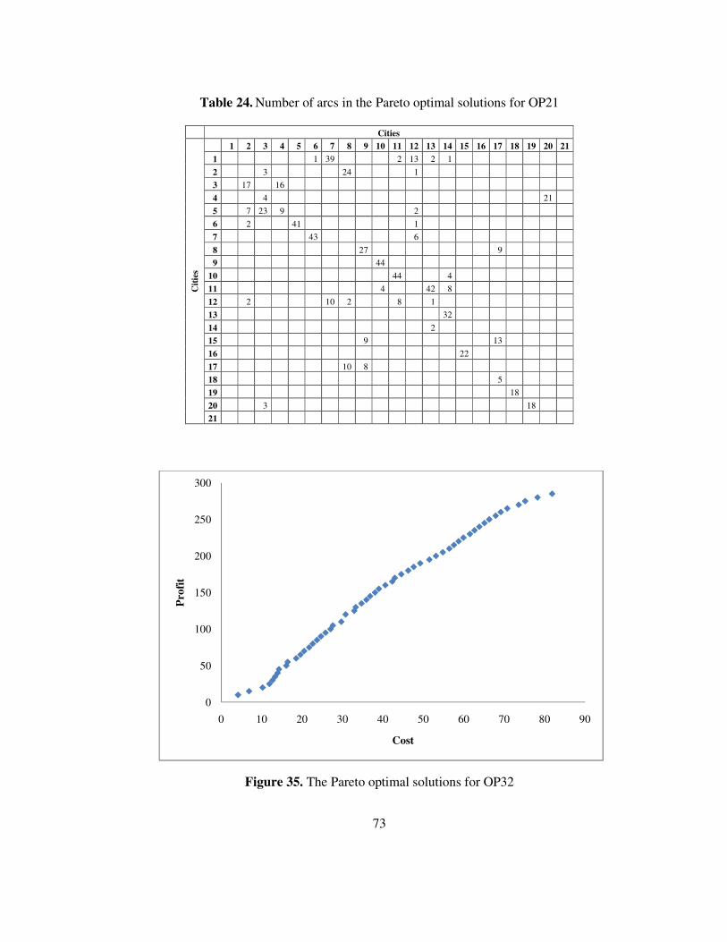
73

Table 24. Number of arcs in the Pareto optimal solutions for OP21

Cities

Cit

ies

1 2 3 4 5 6 7 8 9 10 11 12 13 14 15 16 17 18 19 20 21

1 1 39 2 13 2 1

2 3 24 1

3 17 16

4 4 21

5 7 23 9 2

6 2 41 1

7 43 6

8 27 9

9 44

10 44 4

11 4 42 8

12 2 10 2 8 1

13 32

14 2

15 9 13

16 22

17 10 8

18 5

19 18

20 3 18

21


0

50

100

150

200

250

300

0 10 20 30 40 50 60 70 80 90

Pro

fit

Cost

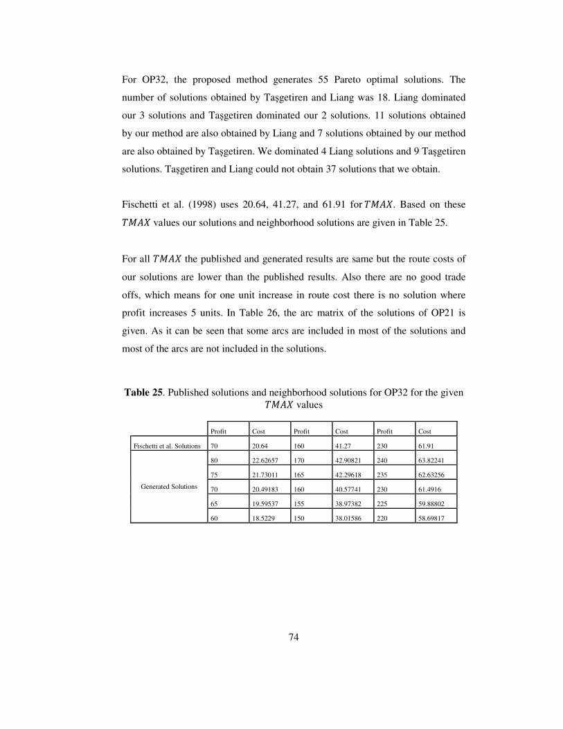
74


number of solutions obtained by Taşgetiren and Liang was 18. Liang dominated

our 3 solutions and Taşgetiren dominated our 2 solutions. 11 solutions obtained

by our method are also obtained by Liang and 7 solutions obtained by our method

are also obtained by Taşgetiren. We dominated 4 Liang solutions and 9 Taşgetiren

solutions. Taşgetiren and Liang could not obtain 37 solutions that we obtain.

Fischetti et al. (1998) uses 20.64, 41.27, and 61.91 for ��. Based on these �� values our solutions and neighborhood solutions are given in Table 25.

For all �� the published and generated results are same but the route costs of

our solutions are lower than the published results. Also there are no good trade

offs, which means for one unit increase in route cost there is no solution where

profit increases 5 units. In Table 26, the arc matrix of the solutions of OP21 is

given. As it can be seen that some arcs are included in most of the solutions and

most of the arcs are not included in the solutions.




Generated Solutions

80 22.62657 170 42.90821 240 63.82241

75 21.73011 165 42.29618 235 62.63256

70 20.49183 160 40.57741 230 61.4916

65 19.59537 155 38.97382 225 59.88802

60 18.5229 150 38.01586 220 58.69817

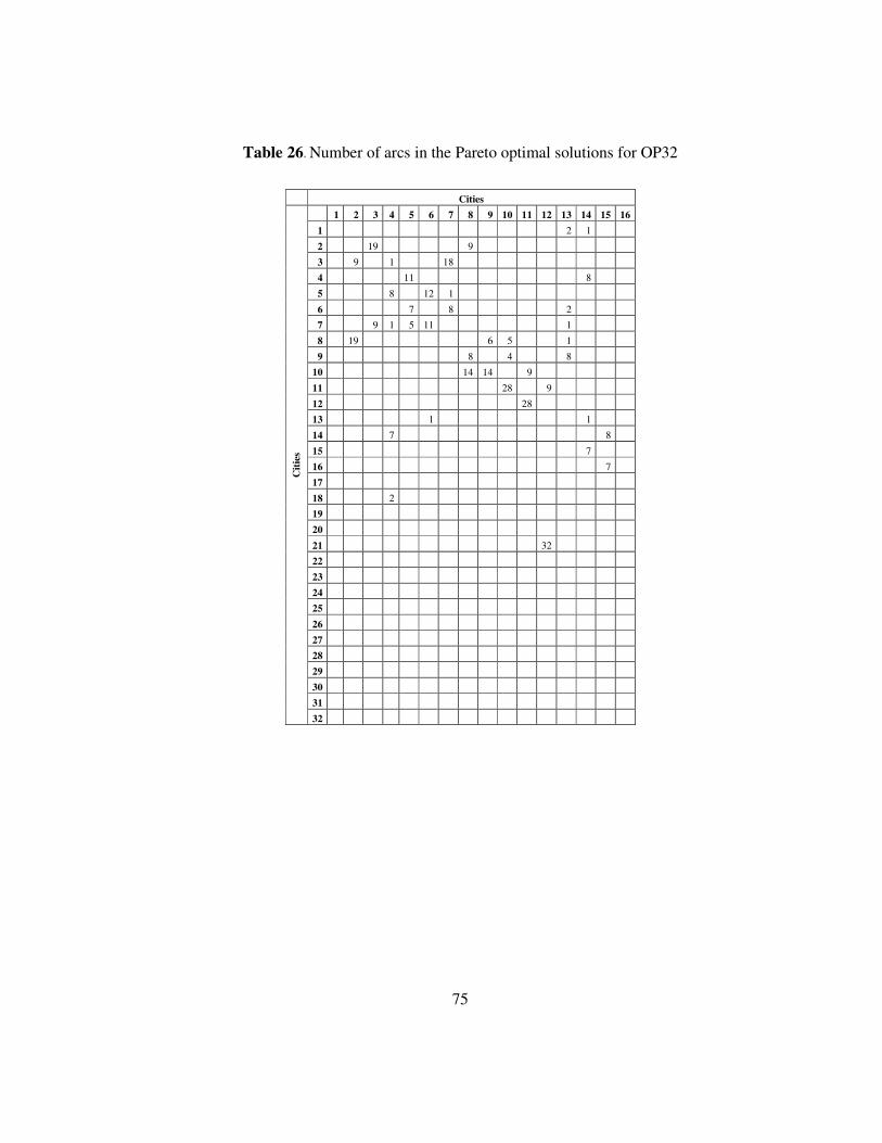
75

Table 26. Number of arcs in the Pareto optimal solutions for OP32

Cities

Cit

ies

1 2 3 4 5 6 7 8 9 10 11 12 13 14 15 16

1 2 1

2 19 9

3 9 1 18

4 11 8

5 8 12 1

6 7 8 2

7 9 1 5 11 1

8 19 6 5 1

9 8 4 8

10 14 14 9

11 28 9

12 28

13 1 1

14 7 8

15 7

16 7

17

18 2

19

20

21 32

22

23

24

25

26

27

28

29

30

31

32

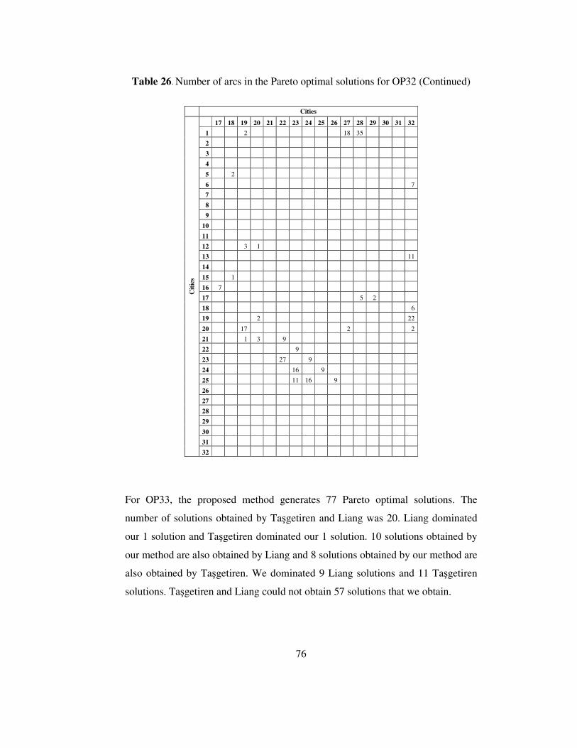
76

Table 26. Number of arcs in the Pareto optimal solutions for OP32 (Continued)

Cities

Cit

ies

17 18 19 20 21 22 23 24 25 26 27 28 29 30 31 32

1 2 18 35

2

3

4

5 2

6 7

7

8

9

10

11

12 3 1

13 11

14

15 1

16 7

17 5 2

18 6

19 2 22

20 17 2 2

21 1 3 9

22 9

23 27 9

24 16 9

25 11 16 9

26

27

28

29

30

31

32


number of solutions obtained by Taşgetiren and Liang was 20. Liang dominated

our 1 solution and Taşgetiren dominated our 1 solution. 10 solutions obtained by

our method are also obtained by Liang and 8 solutions obtained by our method are

also obtained by Taşgetiren. We dominated 9 Liang solutions and 11 Taşgetiren

solutions. Taşgetiren and Liang could not obtain 57 solutions that we obtain.

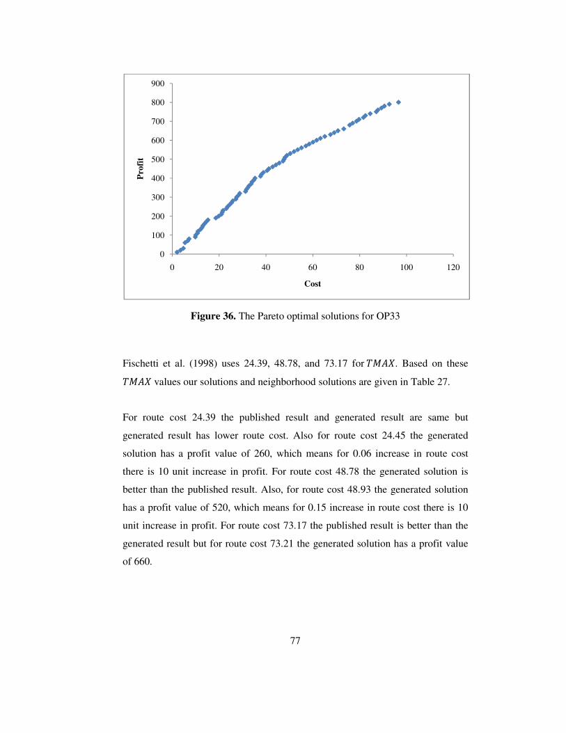
77


Fischetti et al. (1998) uses 24.39, 48.78, and 73.17 for ��. Based on these �� values our solutions and neighborhood solutions are given in Table 27.

For route cost 24.39 the published result and generated result are same but

generated result has lower route cost. Also for route cost 24.45 the generated

solution has a profit value of 260, which means for 0.06 increase in route cost

there is 10 unit increase in profit. For route cost 48.78 the generated solution is

better than the published result. Also, for route cost 48.93 the generated solution

has a profit value of 520, which means for 0.15 increase in route cost there is 10

unit increase in profit. For route cost 73.17 the published result is better than the

generated result but for route cost 73.21 the generated solution has a profit value

of 660.

0

100

200

300

400

500

600

700

800

900

0 20 40 60 80 100 120

Pro

fit

Cost

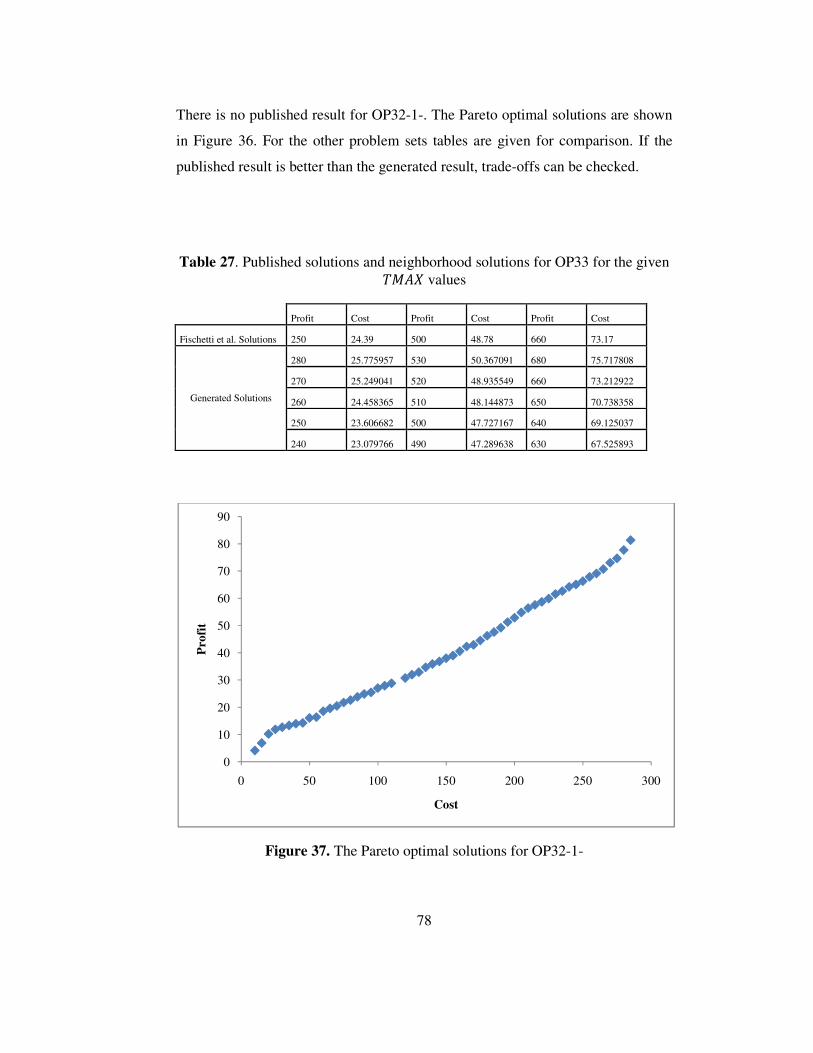
78

There is no published result for OP32-1-. The Pareto optimal solutions are shown

in Figure 36. For the other problem sets tables are given for comparison. If the

published result is better than the generated result, trade-offs can be checked.




Generated Solutions

280 25.775957 530 50.367091 680 75.717808

270 25.249041 520 48.935549 660 73.212922

260 24.458365 510 48.144873 650 70.738358

250 23.606682 500 47.727167 640 69.125037

240 23.079766 490 47.289638 630 67.525893

Figure 37. The Pareto optimal solutions for OP32-1-

0

10

20

30

40

50

60

70

80

90

0 50 100 150 200 250 300

Pro

fit

Cost

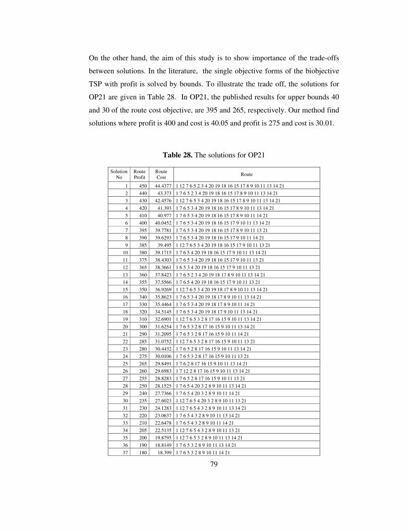
79

On the other hand, the aim of this study is to show importance of the trade-offs

between solutions. In the literature, the single objective forms of the biobjective

TSP with profit is solved by bounds. To illustrate the trade off, the solutions for

OP21 are given in Table 28. In OP21, the published results for upper bounds 40

and 30 of the route cost objective, are 395 and 265, respectively. Our method find

solutions where profit is 400 and cost is 40.05 and profit is 275 and cost is 30.01.

Table 28. The solutions for OP21

Solution No

Route Profit

Route Cost

Route

1 450 44.4377 1 12 7 6 5 2 3 4 20 19 18 16 15 17 8 9 10 11 13 14 21

2 440 43.373 1 7 6 5 2 3 4 20 19 18 16 15 17 8 9 10 11 13 14 21

3 430 42.4576 1 12 7 6 5 3 4 20 19 18 16 15 17 8 9 10 11 13 14 21

4 420 41.393 1 7 6 5 3 4 20 19 18 16 15 17 8 9 10 11 13 14 21

5 410 40.977 1 7 6 5 3 4 20 19 18 16 15 17 8 9 10 11 14 21

6 400 40.0452 1 7 6 5 3 4 20 19 18 16 15 17 9 10 11 13 14 21

7 395 39.7781 1 7 6 5 3 4 20 19 18 16 15 17 8 9 10 11 13 21

8 390 39.6293 1 7 6 5 3 4 20 19 18 16 15 17 9 10 11 14 21

9 385 39.495 1 12 7 6 5 3 4 20 19 18 16 15 17 9 10 11 13 21

10 380 39.1715 1 7 6 5 4 20 19 18 16 15 17 9 10 11 13 14 21

11 375 38.4303 1 7 6 5 3 4 20 19 18 16 15 17 9 10 11 13 21

12 365 38.3661 1 6 5 3 4 20 19 18 16 15 17 9 10 11 13 21

13 360 37.8423 1 7 6 5 2 3 4 20 19 18 17 8 9 10 11 13 14 21

14 355 37.5566 1 7 6 5 4 20 19 18 16 15 17 9 10 11 13 21

15 350 36.9269 1 12 7 6 5 3 4 20 19 18 17 8 9 10 11 13 14 21

16 340 35.8623 1 7 6 5 3 4 20 19 18 17 8 9 10 11 13 14 21

17 330 35.4464 1 7 6 5 3 4 20 19 18 17 8 9 10 11 14 21

18 320 34.5145 1 7 6 5 3 4 20 19 18 17 9 10 11 13 14 21

19 310 32.6901 1 12 7 6 5 3 2 8 17 16 15 9 10 11 13 14 21

20 300 31.6254 1 7 6 5 3 2 8 17 16 15 9 10 11 13 14 21

21 290 31.2095 1 7 6 5 3 2 8 17 16 15 9 10 11 14 21

22 285 31.0752 1 12 7 6 5 3 2 8 17 16 15 9 10 11 13 21

23 280 30.4432 1 7 6 5 2 8 17 16 15 9 10 11 13 14 21

24 275 30.0106 1 7 6 5 3 2 8 17 16 15 9 10 11 13 21

25 265 29.8491 1 7 6 2 8 17 16 15 9 10 11 13 14 21

26 260 29.6983 1 7 12 2 8 17 16 15 9 10 11 13 14 21

27 255 28.8283 1 7 6 5 2 8 17 16 15 9 10 11 13 21

28 250 28.1525 1 7 6 5 4 20 3 2 8 9 10 11 13 14 21

29 240 27.7366 1 7 6 5 4 20 3 2 8 9 10 11 14 21

30 235 27.6023 1 12 7 6 5 4 20 3 2 8 9 10 11 13 21

31 230 24.1283 1 12 7 6 5 4 3 2 8 9 10 11 13 14 21

32 220 23.0637 1 7 6 5 4 3 2 8 9 10 11 13 14 21

33 210 22.6478 1 7 6 5 4 3 2 8 9 10 11 14 21

34 205 22.5135 1 12 7 6 5 4 3 2 8 9 10 11 13 21

35 200 19.8795 1 12 7 6 5 3 2 8 9 10 11 13 14 21

36 190 18.8149 1 7 6 5 3 2 8 9 10 11 13 14 21

37 180 18.399 1 7 6 5 3 2 8 9 10 11 14 21

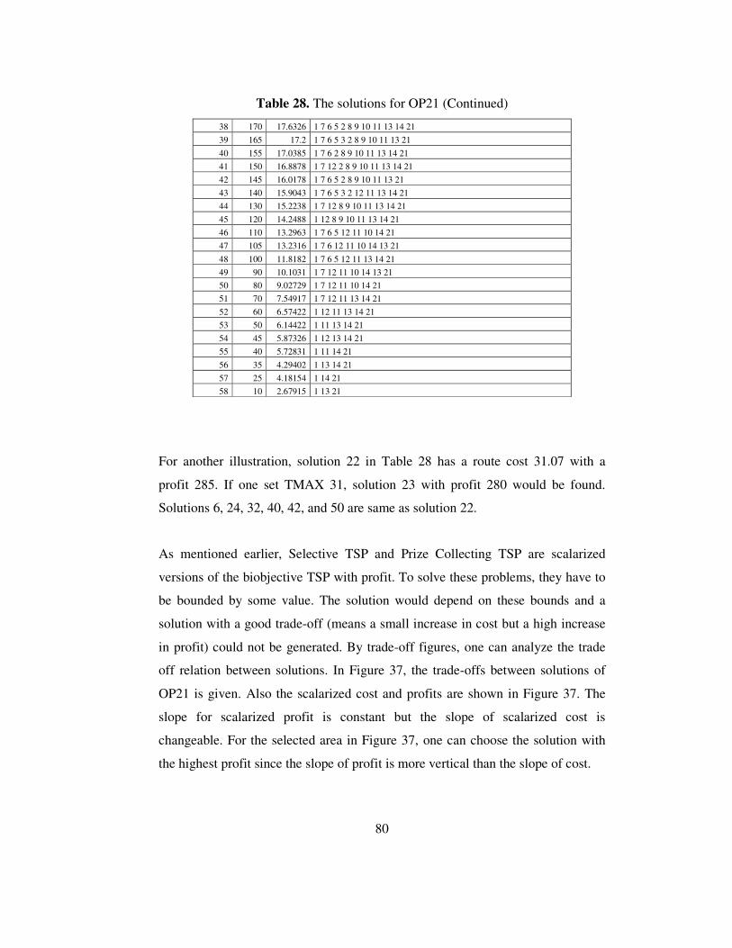
80

Table 28. The solutions for OP21 (Continued)

38 170 17.6326 1 7 6 5 2 8 9 10 11 13 14 21

39 165 17.2 1 7 6 5 3 2 8 9 10 11 13 21

40 155 17.0385 1 7 6 2 8 9 10 11 13 14 21

41 150 16.8878 1 7 12 2 8 9 10 11 13 14 21

42 145 16.0178 1 7 6 5 2 8 9 10 11 13 21

43 140 15.9043 1 7 6 5 3 2 12 11 13 14 21

44 130 15.2238 1 7 12 8 9 10 11 13 14 21

45 120 14.2488 1 12 8 9 10 11 13 14 21

46 110 13.2963 1 7 6 5 12 11 10 14 21

47 105 13.2316 1 7 6 12 11 10 14 13 21

48 100 11.8182 1 7 6 5 12 11 13 14 21

49 90 10.1031 1 7 12 11 10 14 13 21

50 80 9.02729 1 7 12 11 10 14 21

51 70 7.54917 1 7 12 11 13 14 21

52 60 6.57422 1 12 11 13 14 21

53 50 6.14422 1 11 13 14 21

54 45 5.87326 1 12 13 14 21

55 40 5.72831 1 11 14 21

56 35 4.29402 1 13 14 21

57 25 4.18154 1 14 21

58 10 2.67915 1 13 21

For another illustration, solution 22 in Table 28 has a route cost 31.07 with a

profit 285. If one set TMAX 31, solution 23 with profit 280 would be found.

Solutions 6, 24, 32, 40, 42, and 50 are same as solution 22.

As mentioned earlier, Selective TSP and Prize Collecting TSP are scalarized

versions of the biobjective TSP with profit. To solve these problems, they have to

be bounded by some value. The solution would depend on these bounds and a

solution with a good trade-off (means a small increase in cost but a high increase

in profit) could not be generated. By trade-off figures, one can analyze the trade

off relation between solutions. In Figure 37, the trade-offs between solutions of

OP21 is given. Also the scalarized cost and profits are shown in Figure 37. The

slope for scalarized profit is constant but the slope of scalarized cost is

changeable. For the selected area in Figure 37, one can choose the solution with

the highest profit since the slope of profit is more vertical than the slope of cost.

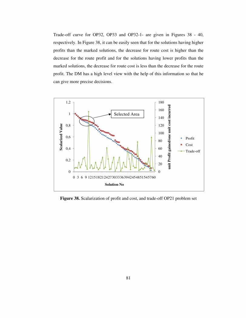
81

Trade-off curve for OP32, OP33 and OP32-1- are given in Figures 38 - 40,

respectively. In Figure 38, it can be easily seen that for the solutions having higher

profits than the marked solutions, the decrease for route cost is higher than the

decrease for the route profit and for the solutions having lower profits than the

marked solutions, the decrease for route cost is less than the decrease for the route

profit. The DM has a high level view with the help of this information so that he

can give more precise decisions.

Figure 38. Scalarization of profit and cost, and trade-off OP21 problem set

0

20

40

60

80

100

120

140

160

180

0

0,2

0,4

0,6

0,8

1

1,2

0 3 6 9 1215182124273033363942454851545760

un

it P

rofi

t ga

ined

/on

e u

nit

cos

t in

curr

ed

Sca

lari

zed

Val

ue

Solution No

Profit

Cost

Trade-off

Selected Area

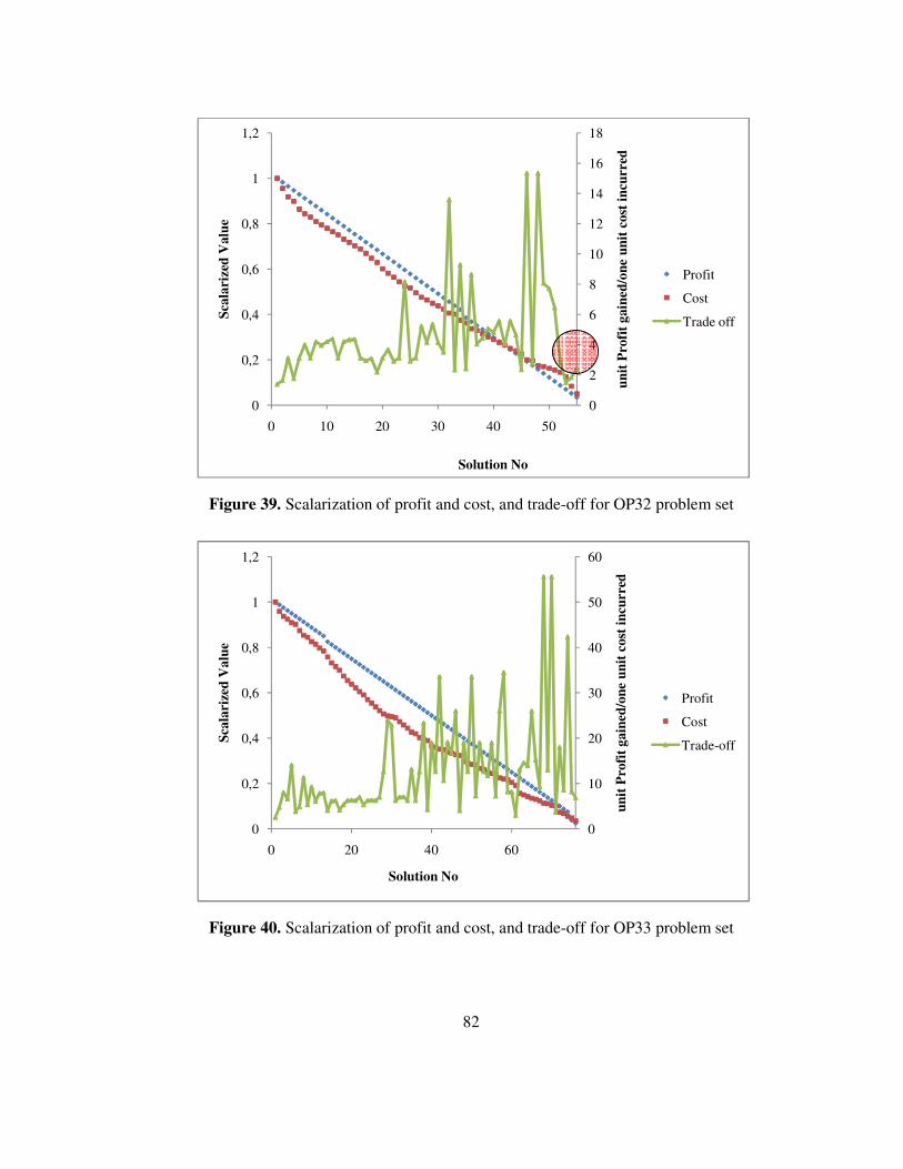
82

Figure 39. Scalarization of profit and cost, and trade-off for OP32 problem set

Figure 40. Scalarization of profit and cost, and trade-off for OP33 problem set

0

2

4

6

8

10

12

14

16

18

0

0,2

0,4

0,6

0,8

1

1,2

0 10 20 30 40 50

un

it P

rofi

t ga

ined

/on

e u

nit

cos

t in

curr

ed

Sca

lari

zed

Val

ue

Solution No

Profit

Cost

Trade off

0

10

20

30

40

50

60

0

0,2

0,4

0,6

0,8

1

1,2

0 20 40 60

un

it P

rofi

t ga

ined

/on

e u

nit

cos

t in

curr

ed

Sca

lari

zed

Val

ue

Solution No

Profit

Cost

Trade-off

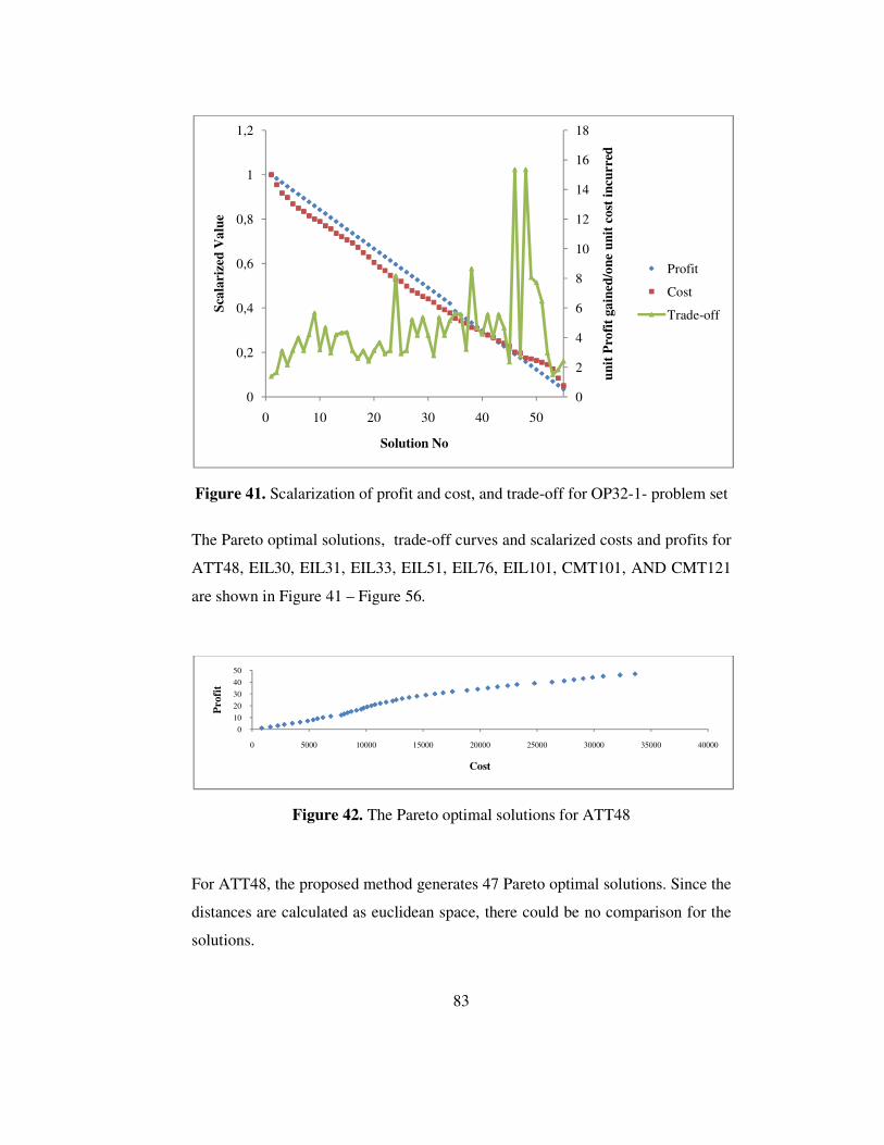
83

Figure 41. Scalarization of profit and cost, and trade-off for OP32-1- problem set

The Pareto optimal solutions, trade-off curves and scalarized costs and profits for

ATT48, EIL30, EIL31, EIL33, EIL51, EIL76, EIL101, CMT101, AND CMT121

are shown in Figure 41 – Figure 56.

Figure 42. The Pareto optimal solutions for ATT48

For ATT48, the proposed method generates 47 Pareto optimal solutions. Since the

distances are calculated as euclidean space, there could be no comparison for the

solutions.

0

2

4

6

8

10

12

14

16

18

0

0,2

0,4

0,6

0,8

1

1,2

0 10 20 30 40 50

un

it P

rofi

t ga

ined

/on

e u

nit

cos

t in

curr

ed

Sca

lari

zed

Val

ue

Solution No

Profit

Cost

Trade-off

0

10

20

30

40

50

0 5000 10000 15000 20000 25000 30000 35000 40000

Pro

fit

Cost

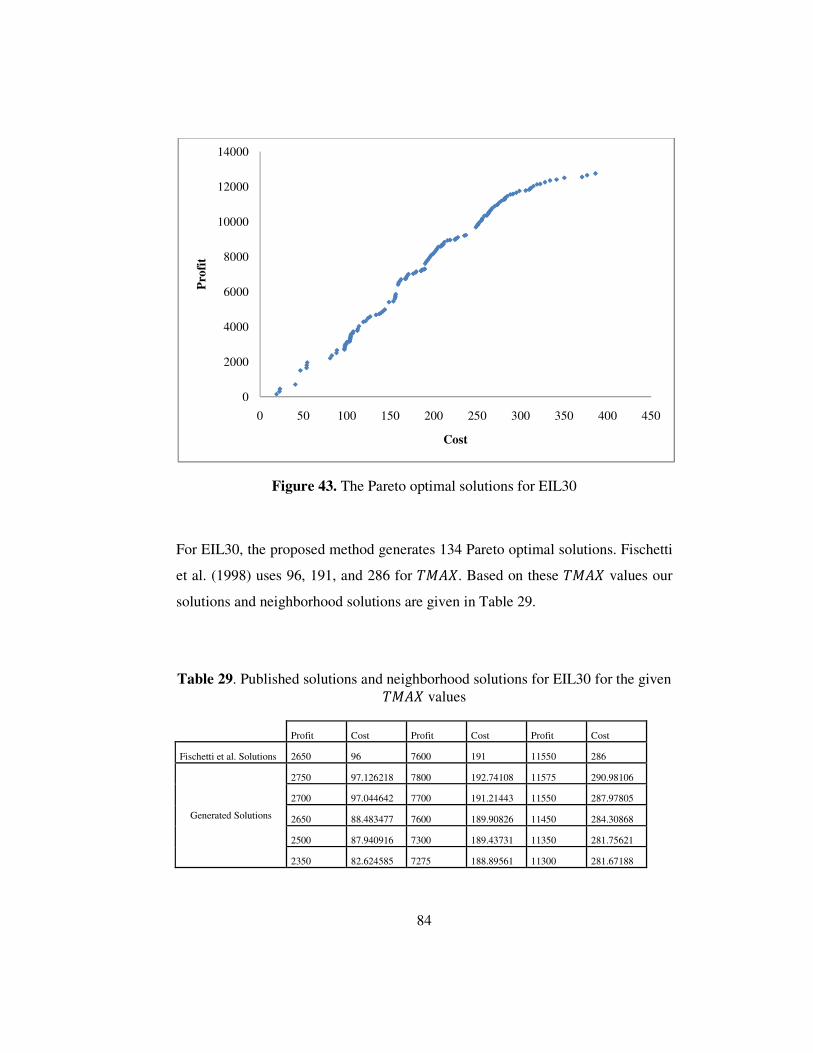
84

Figure 43. The Pareto optimal solutions for EIL30

For EIL30, the proposed method generates 134 Pareto optimal solutions. Fischetti

et al. (1998) uses 96, 191, and 286 for ��. Based on these �� values our

solutions and neighborhood solutions are given in Table 29.

Table 29. Published solutions and neighborhood solutions for EIL30 for the given �� values


Fischetti et al. Solutions 2650 96 7600 191 11550 286

Generated Solutions

2750 97.126218 7800 192.74108 11575 290.98106

2700 97.044642 7700 191.21443 11550 287.97805

2650 88.483477 7600 189.90826 11450 284.30868

2500 87.940916 7300 189.43731 11350 281.75621

2350 82.624585 7275 188.89561 11300 281.67188

0

2000

4000

6000

8000

10000

12000

14000

0 50 100 150 200 250 300 350 400 450

Pro

fit

Cost

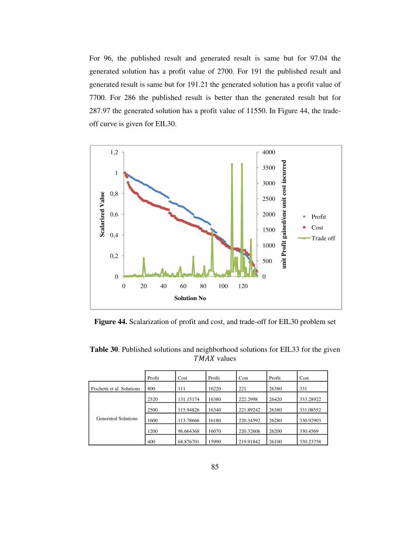
85

For 96, the published result and generated result is same but for 97.04 the

generated solution has a profit value of 2700. For 191 the published result and

generated result is same but for 191.21 the generated solution has a profit value of

7700. For 286 the published result is better than the generated result but for

287.97 the generated solution has a profit value of 11550. In Figure 44, the trade-

off curve is given for EIL30.

Figure 44. Scalarization of profit and cost, and trade-off for EIL30 problem set

Table 30. Published solutions and neighborhood solutions for EIL33 for the given �� values



Generated Solutions

2520 131.15174 16380 222.2998 26420 333.28922

2500 115.94826 16340 221.89242 26380 331.08552

1600 113.78666 16180 220.34592 26280 330.92903

1200 96.664368 16070 220.32606 26200 330.4569

400 68.876701 15990 219.91842 26100 330.23758

0

500

1000

1500

2000

2500

3000

3500

4000

0

0,2

0,4

0,6

0,8

1

1,2

0 20 40 60 80 100 120u

nit

Pro

fit

gain

ed/o

ne

un

it c

ost

incu

rred

Sca

lari

zed

Val

ue

Solution No

Profit

Cost

Trade off

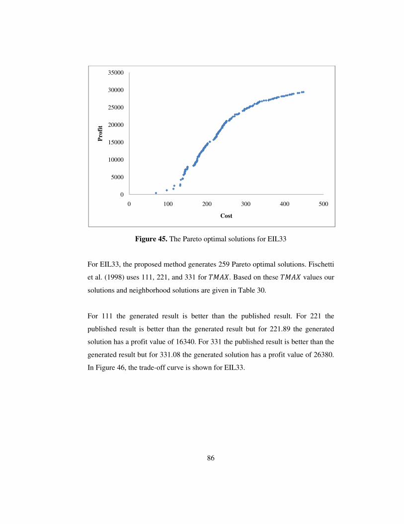
86





For 111 the generated result is better than the published result. For 221 the

published result is better than the generated result but for 221.89 the generated

solution has a profit value of 16340. For 331 the published result is better than the

generated result but for 331.08 the generated solution has a profit value of 26380.

In Figure 46, the trade-off curve is shown for EIL33.

0

5000

10000

15000

20000

25000

30000

35000

0 100 200 300 400 500

Pro

fit

Cost

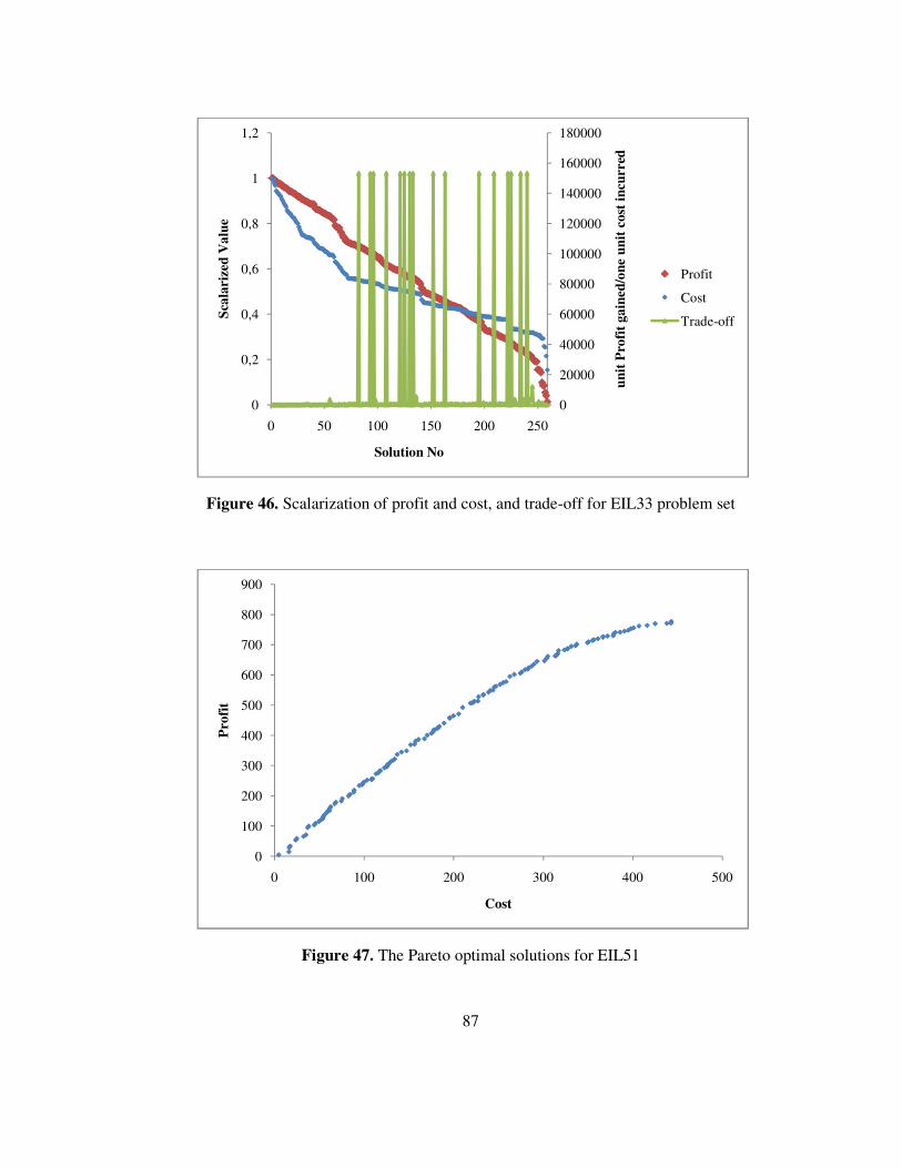
87



0

20000

40000

60000

80000

100000

120000

140000

160000

180000

0

0,2

0,4

0,6

0,8

1

1,2

0 50 100 150 200 250

un

it P

rofi

t ga

ined

/on

e u

nit

cos

t in

curr

ed

Sca

lari

zed

Val

ue

Solution No

Profit

Cost

Trade-off

0

100

200

300

400

500

600

700

800

900

0 100 200 300 400 500

Pro

fit

Cost

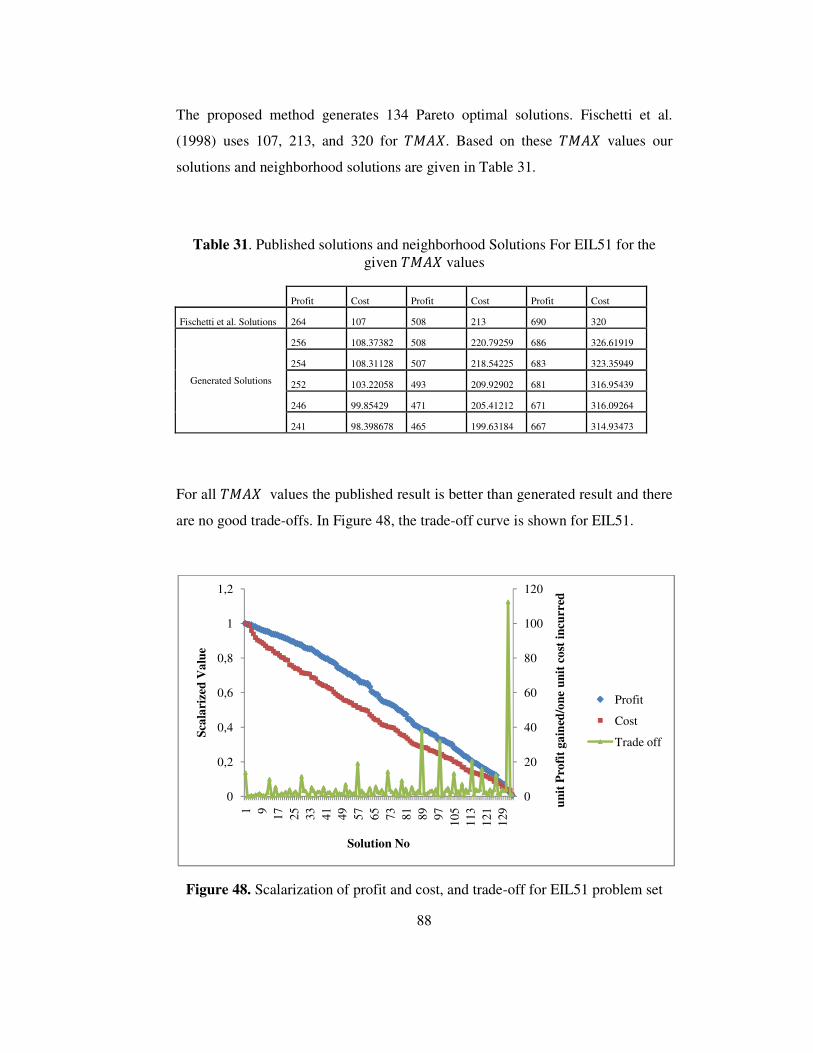
88

The proposed method generates 134 Pareto optimal solutions. Fischetti et al.

(1998) uses 107, 213, and 320 for ��. Based on these �� values our


Table 31. Published solutions and neighborhood Solutions For EIL51 for the given �� values



Generated Solutions

256 108.37382 508 220.79259 686 326.61919

254 108.31128 507 218.54225 683 323.35949

252 103.22058 493 209.92902 681 316.95439

246 99.85429 471 205.41212 671 316.09264

241 98.398678 465 199.63184 667 314.93473

For all �� values the published result is better than generated result and there

are no good trade-offs. In Figure 48, the trade-off curve is shown for EIL51.


0

20

40

60

80

100

120

0

0,2

0,4

0,6

0,8

1

1,2

1 9 17 25 33 41 49 57 65 73 81 89 97 105

113

121

129 u

nit

Pro

fit

gain

ed/o

ne

un

it c

ost

incu

rred

Sca

lari

zed

Val

ue

Solution No

Profit

Cost

Trade off

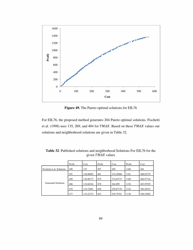
89








Generated Solutions

491 138.06092 881 274.45006 1161 408.02379

490 136.90173 879 274.03737 1160 406.97744

486 134.84544 878 264.899 1154 403.95529

478 134.72891 849 258.87176 1142 396.26543

477 134.22723 843 258.79781 1130 388.43885

0

200

400

600

800

1000

1200

1400

1600

0 100 200 300 400 500 600

Pro

fit

Cost

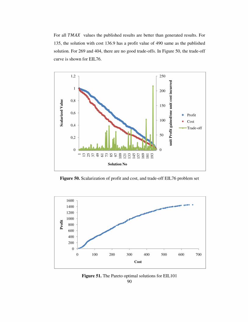
90

For all �� values the published results are better than generated results. For

135, the solution with cost 136.9 has a profit value of 490 same as the published

solution. For 269 and 404, there are no good trade-offs. In Figure 50, the trade-off

curve is shown for EIL76.

Figure 50. Scalarization of profit and cost, and trade-off EIL76 problem set


0

50

100

150

200

250

0

0,2

0,4

0,6

0,8

1

1,21 13 25 37 49 61 73 85 97 109

121

133

145

157

169

181

193

un

it P

rofi

t ga

ined

/on

e u

nit

cos

t in

curr

ed

Sca

lari

zed

Val

ue

Solution No

Profit

Cost

Trade-off

0

200

400

600

800

1000

1200

1400

1600

0 100 200 300 400 500 600 700

Pro

fit

Cost

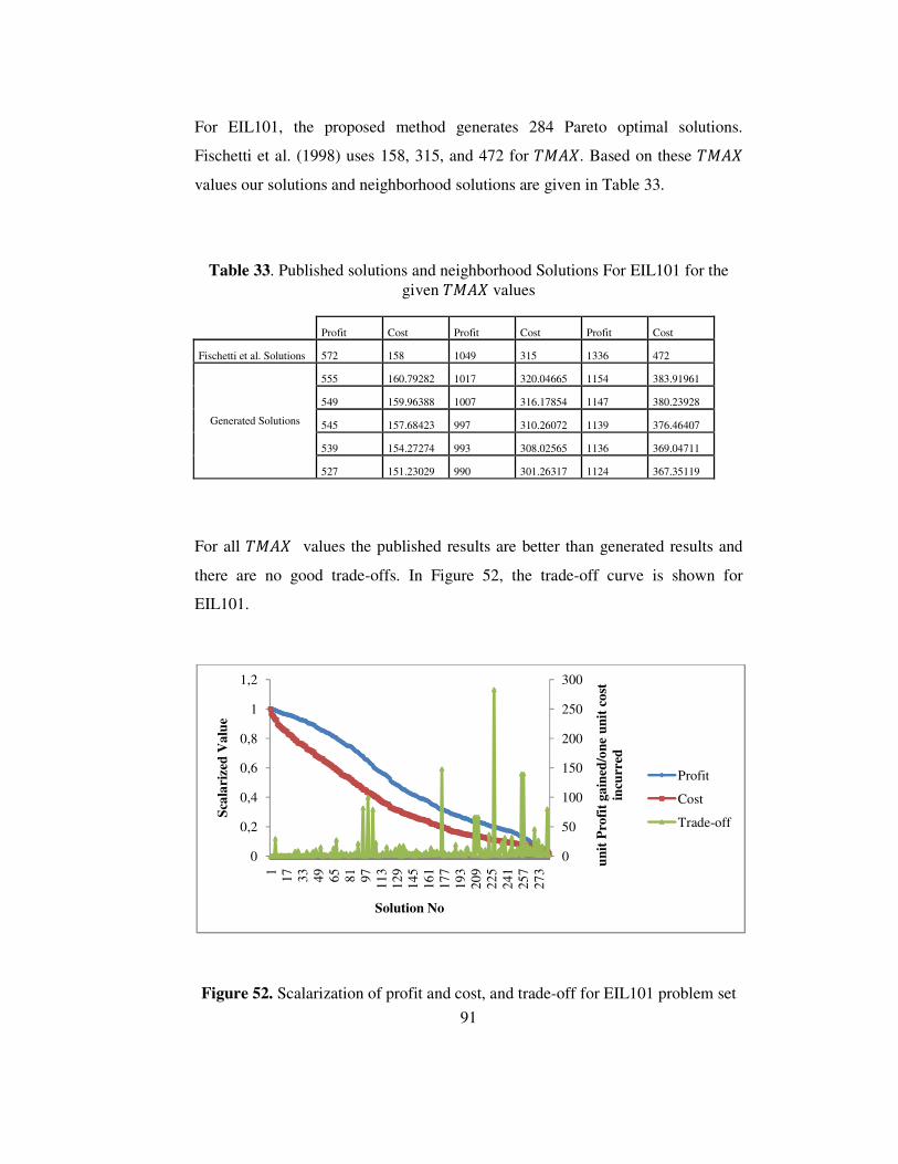
91

For EIL101, the proposed method generates 284 Pareto optimal solutions.

Fischetti et al. (1998) uses 158, 315, and 472 for ��. Based on these ��

values our solutions and neighborhood solutions are given in Table 33.




Generated Solutions

555 160.79282 1017 320.04665 1154 383.91961

549 159.96388 1007 316.17854 1147 380.23928

545 157.68423 997 310.26072 1139 376.46407

539 154.27274 993 308.02565 1136 369.04711

527 151.23029 990 301.26317 1124 367.35119

For all �� values the published results are better than generated results and

there are no good trade-offs. In Figure 52, the trade-off curve is shown for

EIL101.


0

50

100

150

200

250

300

0

0,2

0,4

0,6

0,8

1

1,2

1 17 33 49 65 81 97 113

129

145

161

177

193

209

225

241

257

273

un

it P

rofi

t ga

ined

/on

e u

nit

cos

t in

curr

ed

Sca

lari

zed

Val

ue

Solution No

Profit

Cost

Trade-off

92

Figure 53. The Pareto optimal solutions for CMT101

For CMT101, the proposed method generates 165 Pareto optimal solutions.



Table 34. Published solutions and neighborhood Solutions For CMT101 for the given �� values



Generated Solutions

540 139.19579 1030 255.60207 1500 380.96178

530 128.36219 1020 253.47795 1490 379.23895

510 123.69834 1010 250.87766 1480 377.4826

480 116.95925 1000 247.37919 1470 374.03386

470 114.13082 980 243.38521 1460 373.54206

0

200

400

600

800

1000

1200

1400

1600

1800

2000

0 100 200 300 400 500 600

Pro

fit

Cost

93

For 127, the published solution is better than the generated solution but for 128.36

the generated solution has a profit value of 530. For 253, the published solution is

better than the generated solution but for 253.47 the generated solution has a

profit value of 1020, still worse but a good trade-off. For 379 the solutions are

same but for 379.23 the generated solution has a profit value of 1490. In Figure

54, the trade-off curve is shown for CMT101.

Figure 54. Scalarization of profit and cost, and trade-off for CMT101 problem set

0

10

20

30

40

50

60

70

80

90

0

0,2

0,4

0,6

0,8

1

1,2

1 10 19 28 37 46 55 64 73 82 91 100

109

118

127

136

145

154

163

un

it P

rofi

t ga

ined

/on

e u

nit

cos

t in

curr

ed

Sca

lari

zed

Val

ue

Solution No

Profit

Cost

Trade off

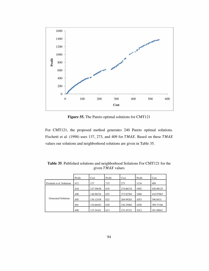
94

Figure 55. The Pareto optimal solutions for CMT121

For CMT121, the proposed method generates 240 Pareto optimal solutions.



Table 35. Published solutions and neighborhood Solutions For CMT121 for the given �� values



Generated Solutions

418 147.59638 635 274.86314 1092 420.98125

408 146.96524 625 273.82584 1068 410.97865

405 136.12438 623 269.99263 1053 396.8431

401 134.60443 620 236.35082 1030 389.37166

400 133.34101 613 233.45321 1012 381.90041

0

200

400

600

800

1000

1200

1400

1600

0 100 200 300 400 500 600

Pro

fit

Cost

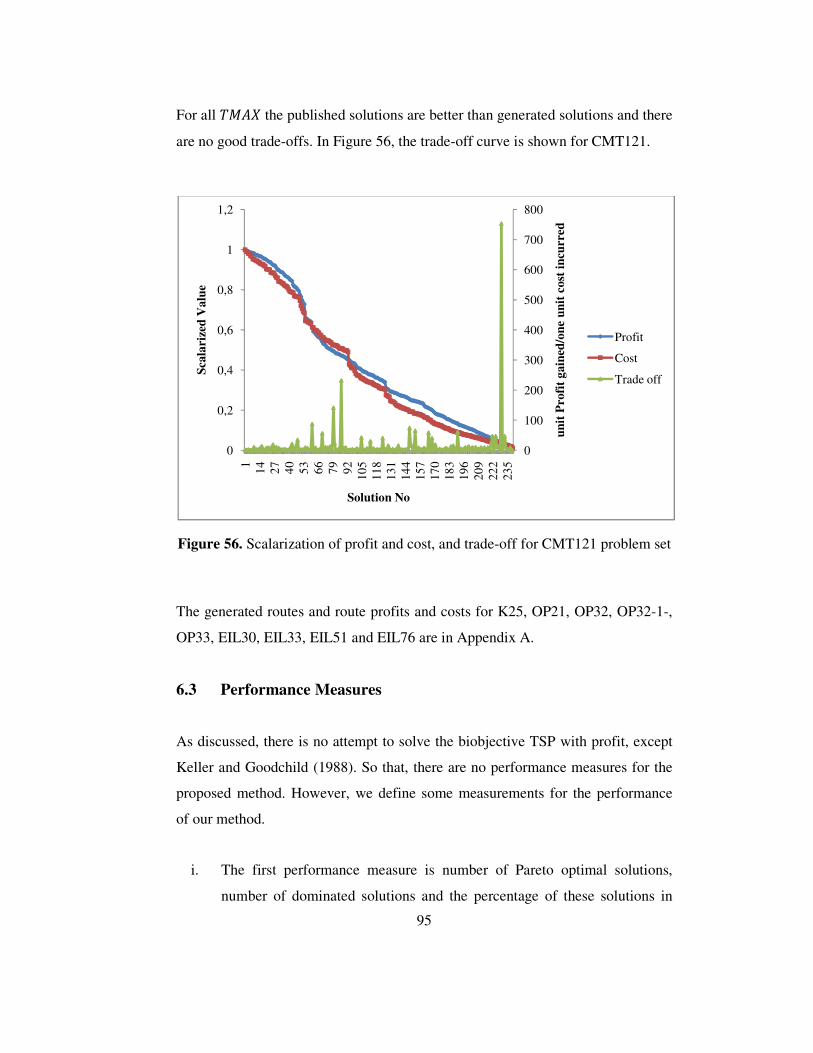
95

For all �� the published solutions are better than generated solutions and there

are no good trade-offs. In Figure 56, the trade-off curve is shown for CMT121.

Figure 56. Scalarization of profit and cost, and trade-off for CMT121 problem set

The generated routes and route profits and costs for K25, OP21, OP32, OP32-1-,

OP33, EIL30, EIL33, EIL51 and EIL76 are in Appendix A.

6.3 Performance Measures

As discussed, there is no attempt to solve the biobjective TSP with profit, except

Keller and Goodchild (1988). So that, there are no performance measures for the

proposed method. However, we define some measurements for the performance

of our method.

i. The first performance measure is number of Pareto optimal solutions,

number of dominated solutions and the percentage of these solutions in

0

100

200

300

400

500

600

700

800

0

0,2

0,4

0,6

0,8

1

1,2

1 14 27 40 53 66 79 92 105

118

131

144

157

170

183

196

209

222

235

un

it P

rofi

t ga

ined

/on

e u

nit

cos

t in

curr

ed

Sca

lari

zed

Val

ue

Solution No

Profit

Cost

Trade off

96

order to measure how effective the method find the Pareto optimal

solutions.

ii. The second performance measure is the time to find a single solution for

the various of number of cities and TMAX for each problem set.

iii. The third performance measure is the total runtime for the problem sets.

For the first performance measure, the number of Pareto optimal solutions and

dominated solutions generated during the solution process for the problem sets. In

Table 36, the first column is the name of the problem sets which already includes

the number of cities for the given problem set. In the second column and third

column, the number of Pareto optimal solutions and dominated solutions are

given, respectively. In the fourth and fifth column, the percentage of dominated

solutions to Pareto optimal solutions and the percentage of Pareto optimal

solutions and total solutions are presented, respectively.

The maximum percentage is for £ / �6 0.61,CMT101. The number of Pareto

optimal solutions and number of dominated solutions does not depend on the size

of the problem set. On the other side, 62% of the generated solutions is Pareto

optimal solutions. CMT101 seems to be bottleneck, so one can conclude that at

least 62% of the generated solutions are Pareto optimal solutions. This table could

be used to evaluate future works.

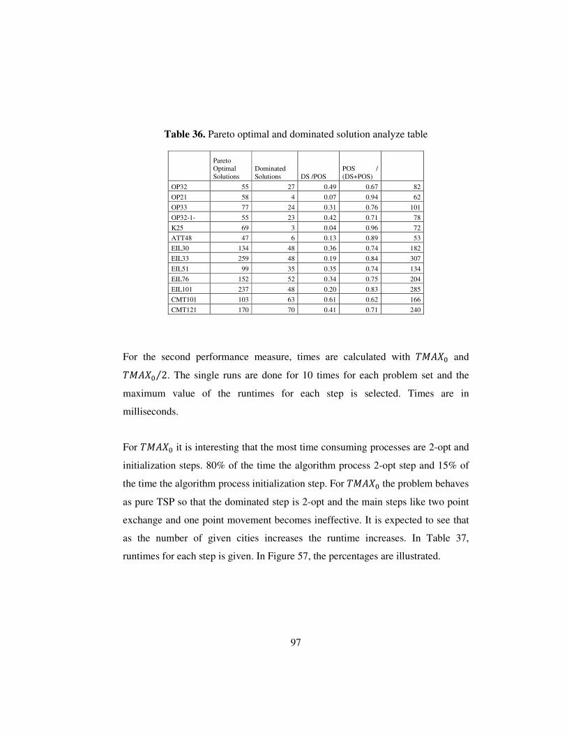
97

Table 36. Pareto optimal and dominated solution analyze table

Pareto Optimal Solutions

Dominated Solutions DS /POS

POS / (DS+POS)

OP32 55 27 0.49 0.67 82

OP21 58 4 0.07 0.94 62

OP33 77 24 0.31 0.76 101

OP32-1- 55 23 0.42 0.71 78

K25 69 3 0.04 0.96 72

ATT48 47 6 0.13 0.89 53

EIL30 134 48 0.36 0.74 182

EIL33 259 48 0.19 0.84 307

EIL51 99 35 0.35 0.74 134

EIL76 152 52 0.34 0.75 204

EIL101 237 48 0.20 0.83 285

CMT101 103 63 0.61 0.62 166

CMT121 170 70 0.41 0.71 240

For the second performance measure, times are calculated with ��: and ��: 2⁄ . The single runs are done for 10 times for each problem set and the

maximum value of the runtimes for each step is selected. Times are in

milliseconds.

For ��: it is interesting that the most time consuming processes are 2-opt and

initialization steps. 80% of the time the algorithm process 2-opt step and 15% of

the time the algorithm process initialization step. For ��: the problem behaves

as pure TSP so that the dominated step is 2-opt and the main steps like two point

exchange and one point movement becomes ineffective. It is expected to see that

as the number of given cities increases the runtime increases. In Table 37,

runtimes for each step is given. In Figure 57, the percentages are illustrated.

98

Figure 57. Time percentages of steps for t¤¥¦§

Table 37. Runtimes for each step for each problem set for a single run with TMAX0

Sequencing Initialization Two Point Exchange

One Point Movement 2 -Opt Reinitialization Total

OP32 0 94 30 0 284 0 408

OP21 0 31 46 16 94 16 203

OP33 0 94 15 0 313 0 422

OP32-1- 0 47 32 0 186 16 281

K25 0 32 14 0 95 0 141

ATT48 0 313 30 0 1017 0 1360

EIL30 0 62 32 0 593 0 687

EIL33 0 47 32 0 343 0 422

EIL51 0 250 62 0 1626 0 1938

EIL76 0 1219 156 0 8531 0 9906

EIL101 0 3578 250 0 23797 0 27625

CMT101 0 3484 218 0 17313 0 21015

CMT121 0 7063 313 15 30531 16 37938

Total 0 16314 1230 31 84723 48 102346

Percentage 0 0.15940047 0.0120181 0.0003029 0.8278096 0.000468997 1

For ��: 2⁄ two point exchange becomes effective and the time percentage of

it increases while the time percentage of 2-opt decreases but still effective. The

other point is that initialization step becomes more dominated then ��:. Now,

50% of time the proposed method processes two point exchange step and 30% of

Sequencing;

0,00%

Initialization;

15,94%

Two Point

Exchange;

1,20%

One Point

Movement;

0,03%

2 -Opt; 82,78%

Reinitialization;

0,05%

Sequencing

Initialization

Two Point Exchange

One Point Movement

2 -Opt

Reinitialization

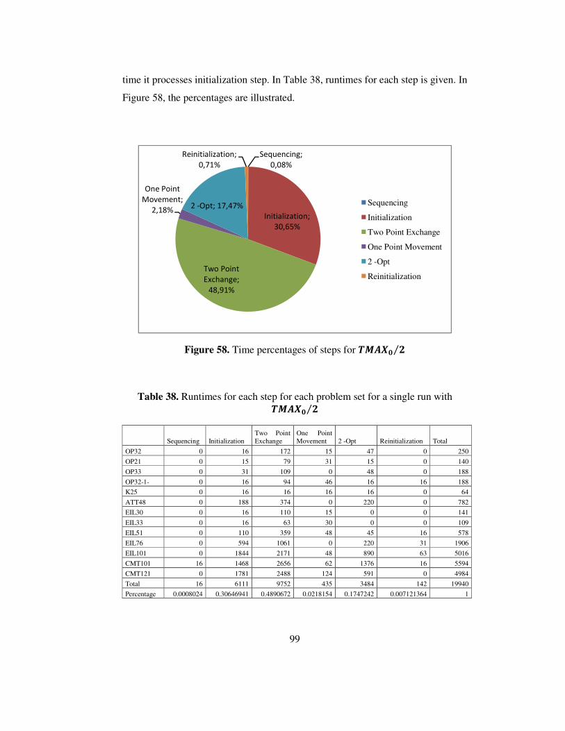
99

time it processes initialization step. In Table 38, runtimes for each step is given. In

Figure 58, the percentages are illustrated.

Figure 58. Time percentages of steps for t¤¥¦§ ¨⁄

Table 38. Runtimes for each step for each problem set for a single run with t¤¥¦§ ¨⁄

Sequencing Initialization Two Point Exchange

One Point Movement 2 -Opt Reinitialization Total

OP32 0 16 172 15 47 0 250

OP21 0 15 79 31 15 0 140

OP33 0 31 109 0 48 0 188

OP32-1- 0 16 94 46 16 16 188

K25 0 16 16 16 16 0 64

ATT48 0 188 374 0 220 0 782

EIL30 0 16 110 15 0 0 141

EIL33 0 16 63 30 0 0 109

EIL51 0 110 359 48 45 16 578

EIL76 0 594 1061 0 220 31 1906

EIL101 0 1844 2171 48 890 63 5016

CMT101 16 1468 2656 62 1376 16 5594

CMT121 0 1781 2488 124 591 0 4984

Total 16 6111 9752 435 3484 142 19940

Percentage 0.0008024 0.30646941 0.4890672 0.0218154 0.1747242 0.007121364 1

Sequencing;

0,08%

Initialization;

30,65%

Two Point

Exchange;

48,91%

One Point

Movement;

2,18%2 -Opt; 17,47%

Reinitialization;

0,71%

Sequencing

Initialization

Two Point Exchange

One Point Movement

2 -Opt

Reinitialization

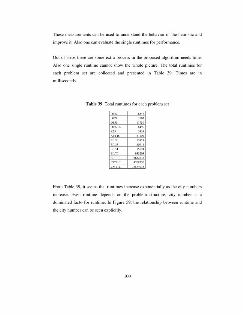
100

These measurements can be used to understand the behavior of the heuristic and

improve it. Also one can evaluate the single runtimes for performance.

Out of steps there are some extra process in the proposed algorithm needs time.

Also one single runtime cannot show the whole picture. The total runtimes for

each problem set are collected and presented in Table 39. Times are in

milliseconds.

Table 39. Total runtimes for each problem set

OP32 8547

OP21 1703

OP33 11750

OP32-1- 8496

K25 3438

ATT48 27109

EIL30 13829

EIL33 30718

EIL51 15694

EIL76 933203

EIL101 9632532

CMT101 4708250

CMT121 13534015

From Table 39, it seems that runtimes increase exponentially as the city numbers

increase. Even runtime depends on the problem structure, city number is a

dominated facto for runtime. In Figure 59, the relationship between runtime and

the city number can be seen explicitly.

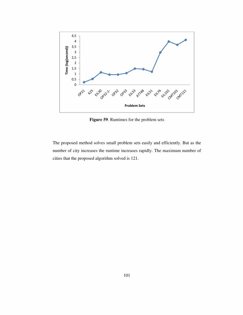
101

Figure 59. Runtimes for the problem sets

The proposed method solves small problem sets easily and efficiently. But as the

number of city increases the runtime increases rapidly. The maximum number of

cities that the proposed algorithm solved is 121.

0

0,5

1

1,5

2

2,5

3

3,5

4

4,5

Tim

e (

log

(se

con

d))

Problem Sets

102

CHAPTER 7

INTERACTIVE SOFTWARE

An interactive software is developed to implement the proposed method. The

software uses data files that contain information about city locations or city

distances and city profits. User can choose starting and ending cities. The software

solves the problem with the choosen starting and ending cities and illustrate the

Pareto optimal solutions in a graphic with an ideal point and subset of efficient

solutions based on the distance formulation and default weights �� d � 0.5 and �z��d � 0.5. Also, only the subset of efficient solutions is illustrated in another

graphic in order to give detail view to the subset of efficient solutions. In another

graphic the trade offs are illustrated between Pareto optimal solutions. User can

define new goal point or weights. The nearest solutions are changed based on the

defined goal point or weights. Detailed information is given about the interactive

software in section 6.1.

7.1 Interactive Software

Software has only one frame, main frame. Main frame contains a map that cities

are illustrated, three graphics that illustrate Pareto optimal solutions, subset of

Pareto optimal solutions and scalarization graphic. In Figure 60, main frame is

shown.

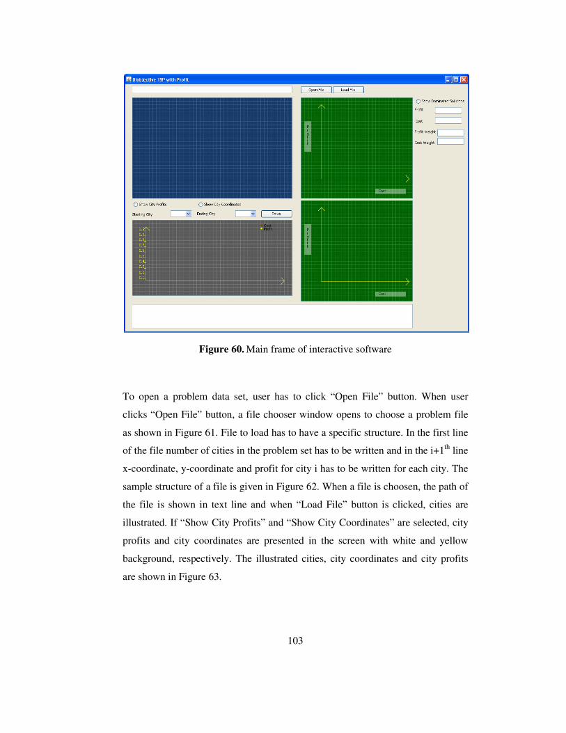
103

Figure 60. Main frame of interactive software

To open a problem data set, user has to click “Open File” button. When user

clicks “Open File” button, a file chooser window opens to choose a problem file

as shown in Figure 61. File to load has to have a specific structure. In the first line

of the file number of cities in the problem set has to be written and in the i+1th line

x-coordinate, y-coordinate and profit for city i has to be written for each city. The

sample structure of a file is given in Figure 62. When a file is choosen, the path of

the file is shown in text line and when “Load File” button is clicked, cities are

illustrated. If “Show City Profits” and “Show City Coordinates” are selected, city

profits and city coordinates are presented in the screen with white and yellow

background, respectively. The illustrated cities, city coordinates and city profits

are shown in Figure 63.

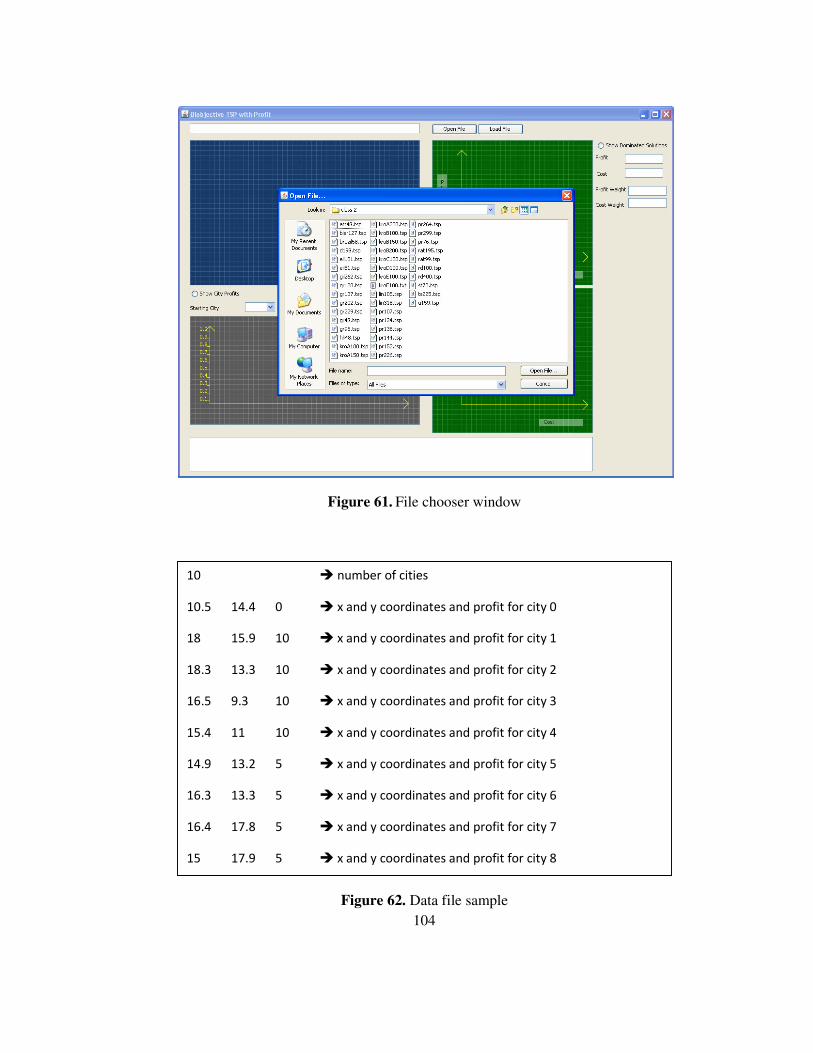
104

Figure 61. File chooser window

Figure 62. Data file sample

10 � number of cities

10.5 14.4 0 � x and y coordinates and profit for city 0

18 15.9 10 � x and y coordinates and profit for city 1



15.4 11 10 � x and y coordinates and profit for city 4




15 17.9 5 � x and y coordinates and profit for city 8

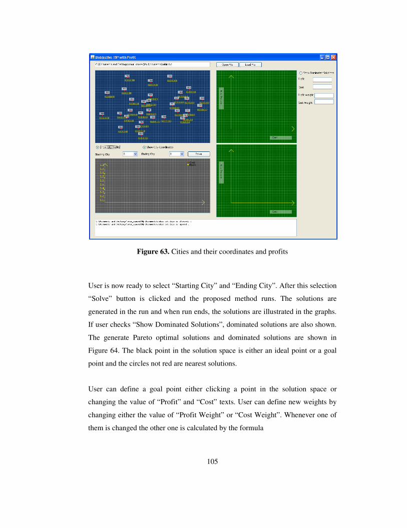
105

Figure 63. Cities and their coordinates and profits

User is now ready to select “Starting City” and “Ending City”. After this selection

“Solve” button is clicked and the proposed method runs. The solutions are

generated in the run and when run ends, the solutions are illustrated in the graphs.

If user checks “Show Dominated Solutions”, dominated solutions are also shown.

The generate Pareto optimal solutions and dominated solutions are shown in

Figure 64. The black point in the solution space is either an ideal point or a goal

point and the circles not red are nearest solutions.

User can define a goal point either clicking a point in the solution space or

changing the value of “Profit” and “Cost” texts. User can define new weights by

changing either the value of “Profit Weight” or “Cost Weight”. Whenever one of

them is changed the other one is calculated by the formula

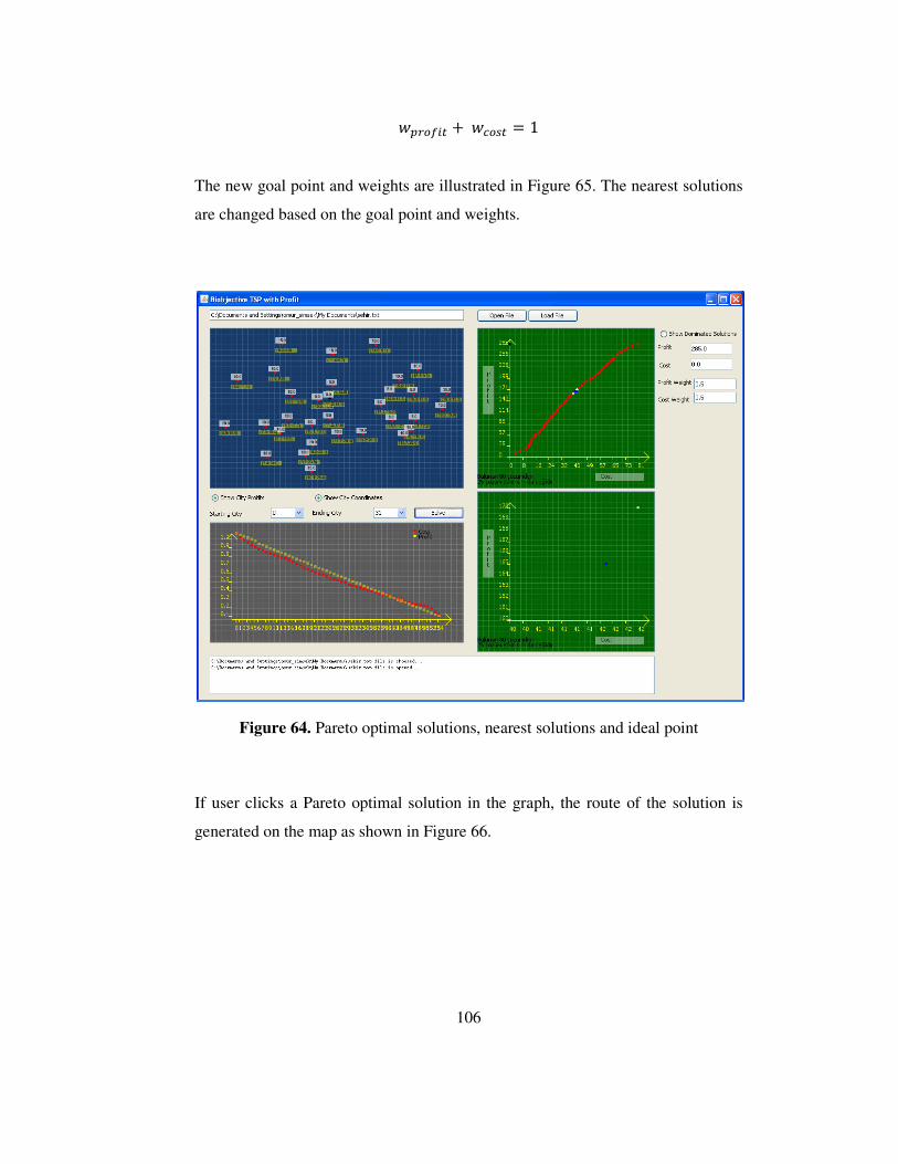
106

�� d T �z��d � 1

The new goal point and weights are illustrated in Figure 65. The nearest solutions

are changed based on the goal point and weights.

Figure 64. Pareto optimal solutions, nearest solutions and ideal point

If user clicks a Pareto optimal solution in the graph, the route of the solution is

generated on the map as shown in Figure 66.

107

Figure 65 Updated goal point, weights and nearest solutions

Figure 66 Route generation on the map

108

CHAPTER 8

CONCLUSION

TSP with profit is naturally biobjective problem where objectives are

contradictory. In the literature single objective TSP with profits are studied. The

only attempt to solve the biobjective TSP with profit is Keller and Goodchild

(1988). In this study we developed a multiobjective approach based on �-

constraint method to solve biobjective TSP with profit. �-constraint method is

chosen because it transforms the problem into single objective problem that is

studied widely in the literature. Since Selective TSP is more widely studied than

Prize Collecting TSP, Selective TSP version of the scalarization is choosen to

study. CGW heuristic, which is fast and effective heuristic, is one of the best

solution methods that solve Selective TSP. To solve the single objective problem,

CGW heuristic is choosen. The computational analysis show that proposed

method performs well. Our study shows that Keller’s algorithm, the only

multiobjective approach for biobjective TSP with Profit, is not good enough to

find Pareto optimal solutions.

An interactive software is developed based on the proposed method. The aim to

develop an interactive software is to give a better understanding about Pareto

optimal solutions to the user. User can change goal points or weights and see how

the subset of efficient solutions changes. Also user can analyze the slope of

decreases or increases of profit and cost by scalarization graphic.

109

For the future work, the proposed method can store all the solutions that is

generated not only best solutions but the bad solutions generated for specific

upper bounds. The bad solutions for a specific upper bound can be Pareto optimal

solutions for other upper bounds. Also the solution set including best solution and

other solutions for a specific upper bound can be used an initial solution for the

updated upper bound.

The interactive software tries to generate all the Pareto optimal solutions. Instead

of this, to increase the performance of the proposed method, subsets of Pareto

optimal solutions can be generated. Considering these solutions and the goal point

and weights defined by user, Pareto optimal solutions between specific limits of

upper bound can be generated. So that the user only gets the information he needs.

Also, the proposed method does not try to generate all the Pareto optimal

solutions. The runtime of the propose method is expected to decrease, especially

for the large problems.

The algorithm mostly uses 2-opt when the problem is almost TSP. So the

performance of the algorithm decreases. One can use Concorde (or any other TSP

solver) instead of 2-opt procedure in the algorithm to improve the solution.

110

REFERENCES

Balas, E. 1989. The prize collecting traveling salesman problem. Networks 19(6)

621–636.

Balas, E. 1995. The prize collecting traveling salesman problem. II: Polyhedral

results. Networks 25(4) 199–216.

Balas, E. 1999. New classes of efficiently solvable generalized travelingsalesman

problems. Ann. Oper. Res. 86 529–558.

Balas, E., G. Martin. 1985. Roll-a-Round: Software Package for Scheduling the

Rounds of a Rolling Mill. Balas and Martin Associates.

Bienstock, D., M. Goemans, D. Simchi-Levi, D. Williamson. 1993. A note on the

prize collecting traveling salesman problem. Math. Programming 59 413–420.

Chao, I.-M., B. L. Golden, E. A. Wasil. 1996. A fast and effective heuristic for the

orienteering problem. Eur. J. Oper. Res. 88(3) 475–489.

Dell’Amico, M., F. Maffioli, A. Sciomachen. 1998. A Lagrangian heuristic for the

prize-collecting travelling salesman problem. Ann. Oper. Res. 81 289–305.

Dell’Amico, M., F. Maffioli, P. Värbrand. 1995. On prize-collecting tours and the

asymmetric travelling salesman problem. Internat.Trans. Oper. Res. 2(3) 297–

308.

Dueck, G. 1990. New optimization heuristics: The great deluge algorithm and the

record-to-record travel. J. Comput. Physics 104(1) 86–92.

111

Ehrgott, M. 2000. Approximation algorithms for combinatorial multicriteria

optimization problems. Internat. Trans. Oper. Res. 7(1) 5–31.

Feillet, D., Dejax P., Gendreau, M. 2005. Traveling Salesman Problems with

Profits. Transportation Science 39(2) 188-205

Fischetti, M., P. Toth. 1988. An additive approach for the optimal solution of the

prize-collecting traveling salesman problem.

Fischetti, M., J. J. Salazar González, P. Toth. 1998. Solving the orienteering

problem through branch-and-cut. INFORMS J. Comput.10(2) 133–148.

Gendreau, M., G. Laporte, F. Semet. 1998a. A branch-and-cut algorithm for the

undirected selective traveling salesman problem. Networks 32 263–273.

Gendreau, M., G. Laporte, F. Semet. 1998b. A tabu search heuristic for the

undirected selective traveling salesman problem. Eur. J.Oper. Res. 106 539–545.

Golden, B. L., L. Levy, R. Vohra. 1987. The orienteering problem. Naval Res.

Logist. 34(3) 307–318.

Golden, B. L., Q. Wang, L. Liu. 1988. A multifaceted heuristic for the

orienteering problem. Naval Res. Logist. 35 359–366.

Göthe-Lundgren, M., K. Jörnsten, P. Värbrand. 1996. On the nucleolus of the

basic vehicle routing game. Math. Programming 72 83–100.

Göthe-Lundgren, M., F. Maffioli, P. Värbrand. 1995. A Lagrangian

decomposition approach for a prize collecting traveling salesman type problem.

Technical Report LiTH-MATH-R-1995-10, Linköping Institute of Technology,

Linköping, Sweden.

112

Gutin, G., A. Punnen, eds. 2002. Traveling Salesman Problem and Its Variations.

Kluwer Academic Publishers, Dordrecht, The Netherlands. Helmberg, C. 1999.

The m-cost ATSP. Lecture Notes Comput. Sci. 1610 242–258.

Kabadi, S. N., A. Punnen. 1996. Prize-collecting traveling salesman problem.

INFORMS Washington Conf., Washington, D.C.

Keller, C. P., M. Goodchild. 1988. The multiobjective vending problem: A

generalization of the traveling salesman problem. Environ. Planning B: Planning

Design 15 447–460.

Laporte, G., S. Martello. 1990. The selective traveling salesman problem.

Discrete Appl. Math. 26 193–207.

Lawler, E.L., Lenstra, J.K., Rinnooy Kan, A.H.G., Shmoys, D.B. (eds,), 1985. The

traveling salesman problem, Wiley, Chichester

Liang, Y.-C., A. E. Smith. 2001. An ant colony approach to the orienteering

problem. Technical report. Department of Industrial and Systems Engineering,

Auburn University, Auburn, AL.

Ramesh, R., K. M. Brown. 1991. An efficient four-phase heuristic for the

generalized orienteering problem. Comput. Oper. Res. 18(2) 151–165.

Ramesh, R., Y.-S. Yoon, M. H. Karwan. 1992. An optimal algorithm for the

orienteering tour problem. ORSA J. Comput. 4(2) 155–165.

Tasgetiren, F. M., A. E. Smith. 2000. A genetic algorithm for the orienteering

problem. Proc. 2000 Congress Evolutionary Comput., San Diego, CA, 1190–

1195.

113

Tsiligirides, T. 1984. Heuristic methods applied to orienteering. J. Oper. Res. Soc.

35(9) 797–809.

Wang, Q., X. Sun, B. L. Golden, J. Jia. 1995. Using artificial neural networks to

solve the orienteering problem. Ann. Oper. Res. 61 111–120

114

APPENDIX

SOLUTIONS OF THE EXPERIMENTAL PROBLEMS

Table A1. The solutions for K25

Route Profit Route Cost Route

13298 3496 5 18 1 8 9 7 4 16 15 6 10 17 14 3 21 23 22 20 13 2 25 12 24 19 11 5

13268 3345 5 18 1 8 9 7 4 16 15 6 17 10 14 3 21 23 22 20 2 25 12 24 19 11 5

13258 3350 5 18 1 8 9 7 4 16 15 6 14 10 17 3 21 23 20 13 2 25 12 24 19 11 5

13228 3199 5 18 1 8 9 7 4 16 15 6 14 10 17 3 21 23 20 2 25 12 24 19 11 5

13178 3064 5 18 1 8 9 7 4 16 15 6 14 17 3 21 23 20 2 25 12 24 19 11 5

13054 2993 5 18 1 8 9 7 4 16 15 6 10 17 14 3 21 23 20 2 25 24 19 11 5

13004 2887 5 18 1 8 9 7 4 16 15 6 14 17 3 21 23 20 2 25 19 24 11 5

12873 2826 5 18 1 8 9 7 4 16 15 6 14 17 3 21 20 2 25 19 24 11 5

12800 2713 5 18 1 8 9 7 4 15 6 14 17 3 21 23 20 2 25 19 24 11 5

12799 2644 5 18 1 8 9 7 4 16 15 6 14 17 3 21 23 20 2 25 19 11 5

12668 2583 5 18 1 8 9 7 4 16 15 6 14 17 3 21 20 2 25 19 11 5

12595 2470 5 18 1 8 9 7 4 15 6 14 17 3 21 23 20 2 25 19 11 5

12464 2409 5 18 1 8 9 7 4 15 6 14 17 3 21 20 2 25 19 11 5

12407 2370 5 18 1 8 9 7 4 16 15 6 14 3 21 20 2 25 19 11 5

12334 2257 5 18 1 8 9 7 4 15 6 14 3 21 23 20 2 25 19 11 5

12203 2196 5 18 1 8 9 7 4 15 6 14 3 21 20 2 25 19 11 5

12092 2161 5 18 8 9 7 4 15 6 14 3 21 23 20 2 25 19 11 5

11961 2100 5 18 8 9 7 4 15 6 14 3 21 20 2 25 19 11 5

11713 2093 5 18 8 9 7 4 15 6 14 3 21 20 25 19 11 5

11646 2086 5 11 19 25 2 20 21 3 14 6 15 7 9 8 18 5

11411 2026 5 11 19 25 2 20 21 3 14 6 4 7 9 8 18 5

11390 2024 5 18 8 9 7 4 15 14 3 21 20 2 25 19 11 5

11163 2019 5 18 8 9 7 4 6 14 3 21 20 25 19 11 5

11142 2017 5 18 8 9 7 4 15 14 3 21 20 25 19 11 5

11096 2012 5 18 8 9 7 6 14 3 21 20 2 25 19 11 5

11075 2010 5 18 8 9 7 15 14 3 21 20 2 25 19 11 5

10827 2003 5 18 8 9 7 15 14 3 21 20 25 19 11 5

10643 1996 5 18 1 8 9 7 4 15 6 14 3 21 25 19 11 5

10401 1900 5 11 19 25 21 3 14 6 15 4 7 9 8 18 5

10089 1893 5 18 8 9 7 4 15 6 14 3 21 25 11 5

10086 1886 5 18 8 9 7 15 6 14 3 21 25 19 11 5

9851 1826 5 18 8 9 7 4 6 14 3 21 25 19 11 5

9830 1824 5 11 19 25 21 3 14 15 4 7 9 8 18 5

9736 1817 5 11 21 3 14 6 15 4 7 9 8 1 18 5

9536 1812 5 18 8 9 7 6 14 3 21 25 19 11 5

9515 1810 5 18 8 9 7 15 14 3 21 25 19 11 5

9514 1786 5 18 8 9 7 4 6 14 3 15 16 11 19 5

9494 1721 5 18 8 9 7 4 15 6 14 3 21 11 5

115

Table A1. The solutions for K25 (Continued)

9202 1642 5 18 8 9 7 4 6 14 3 15 16 11 5

8998 1623 5 18 8 9 7 4 15 6 14 3 11 5

8683 1613 5 18 8 9 7 6 14 3 15 11 5

8652 1573 5 18 8 9 7 4 6 14 3 16 11 5

8609 1511 5 1 8 9 7 4 6 14 3 15 18 5

8367 1422 5 8 9 7 4 6 14 3 15 18 5

8052 1408 5 8 9 7 15 3 14 6 18 5

7547 1367 5 18 8 9 7 4 6 14 15 16 11 19 5

7477 1319 5 18 1 8 9 7 4 6 14 15 16 11 5

7273 1304 5 11 15 14 6 4 7 9 8 1 18 5

7235 1223 5 11 16 15 14 6 4 7 9 8 18 5

7031 1208 5 11 15 14 6 4 7 9 8 18 5

6642 1092 5 1 8 9 7 4 6 14 15 18 5

6400 1003 5 8 9 7 4 6 14 15 18 5

6085 989 5 8 9 7 15 14 6 18 5

5535 984 5 18 6 14 7 9 8 5

5514 982 5 18 15 14 7 9 8 5

5067 974 5 18 7 4 6 14 15 5

4956 909 5 18 8 9 7 4 15 16 11 5

4752 894 5 18 8 9 7 4 15 11 5

4692 841 5 8 9 7 15 6 4 18 5

4444 795 5 18 1 8 9 7 4 11 5

4406 753 5 18 8 9 7 4 16 11 5

4202 699 5 11 4 7 9 8 18 5

4129 680 5 18 1 8 9 7 11 5

3887 584 5 18 7 9 8 11 5

3813 564 5 18 4 7 9 8 1 5

3571 475 5 18 4 7 9 8 5

3498 347 5 18 7 9 8 1 5

3256 258 5 18 7 9 8 5

2628 211 5 18 8 9 5

1969 204 5 18 9 5

1954 152 5 18 8 5

1295 56 5 18 5

Table A2. The solutions for OP21


450 44.44 1 12 7 6 5 2 3 4 20 19 18 16 15 17 8 9 10 11 13 14 21

440 43.37 1 7 6 5 2 3 4 20 19 18 16 15 17 8 9 10 11 13 14 21

430 42.46 1 12 7 6 5 3 4 20 19 18 16 15 17 8 9 10 11 13 14 21

420 41.39 1 7 6 5 3 4 20 19 18 16 15 17 8 9 10 11 13 14 21

410 40.98 1 7 6 5 3 4 20 19 18 16 15 17 8 9 10 11 14 21

400 40.05 1 7 6 5 3 4 20 19 18 16 15 17 9 10 11 13 14 21

395 39.78 1 7 6 5 3 4 20 19 18 16 15 17 8 9 10 11 13 21

390 39.63 1 7 6 5 3 4 20 19 18 16 15 17 9 10 11 14 21

385 39.49 1 12 7 6 5 3 4 20 19 18 16 15 17 9 10 11 13 21

380 39.17 1 7 6 5 4 20 19 18 16 15 17 9 10 11 13 14 21

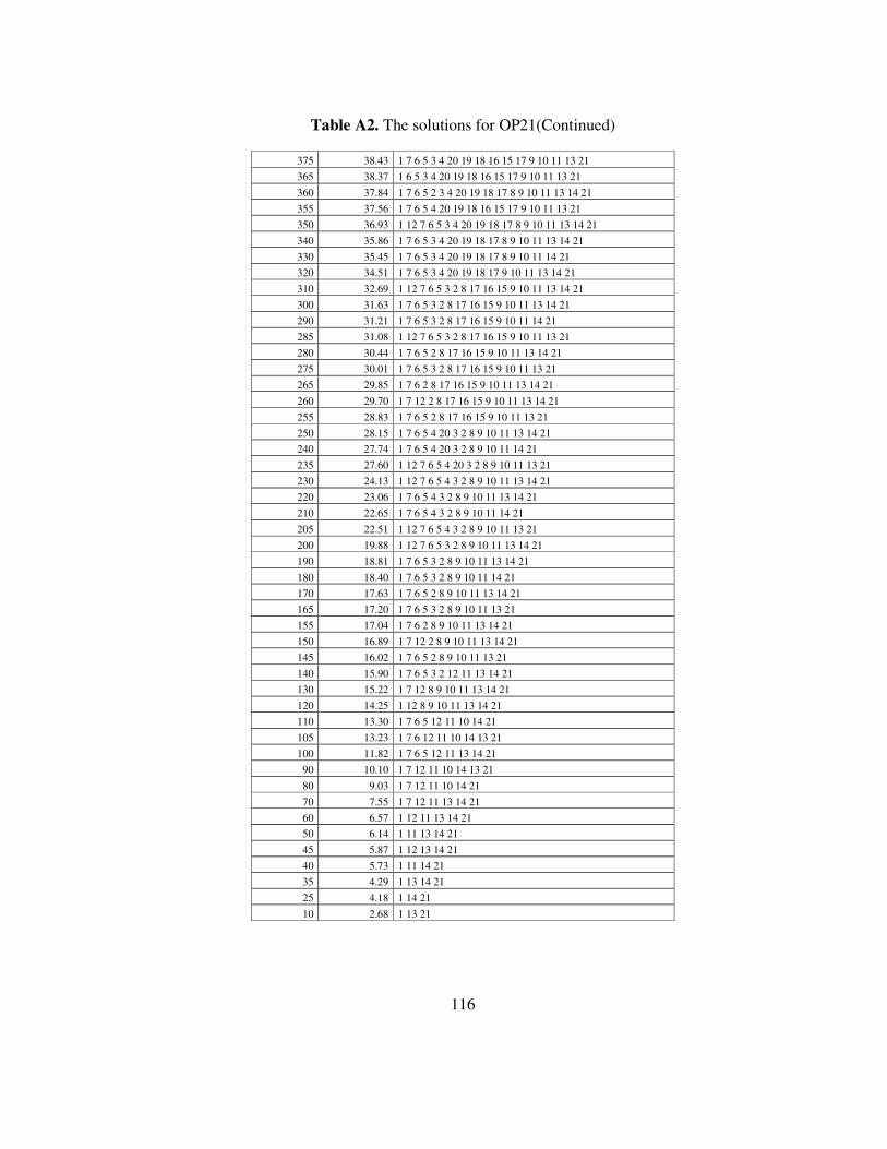
116

Table A2. The solutions for OP21(Continued)

375 38.43 1 7 6 5 3 4 20 19 18 16 15 17 9 10 11 13 21

365 38.37 1 6 5 3 4 20 19 18 16 15 17 9 10 11 13 21

360 37.84 1 7 6 5 2 3 4 20 19 18 17 8 9 10 11 13 14 21

355 37.56 1 7 6 5 4 20 19 18 16 15 17 9 10 11 13 21

350 36.93 1 12 7 6 5 3 4 20 19 18 17 8 9 10 11 13 14 21

340 35.86 1 7 6 5 3 4 20 19 18 17 8 9 10 11 13 14 21

330 35.45 1 7 6 5 3 4 20 19 18 17 8 9 10 11 14 21

320 34.51 1 7 6 5 3 4 20 19 18 17 9 10 11 13 14 21

310 32.69 1 12 7 6 5 3 2 8 17 16 15 9 10 11 13 14 21

300 31.63 1 7 6 5 3 2 8 17 16 15 9 10 11 13 14 21

290 31.21 1 7 6 5 3 2 8 17 16 15 9 10 11 14 21

285 31.08 1 12 7 6 5 3 2 8 17 16 15 9 10 11 13 21

280 30.44 1 7 6 5 2 8 17 16 15 9 10 11 13 14 21

275 30.01 1 7 6 5 3 2 8 17 16 15 9 10 11 13 21

265 29.85 1 7 6 2 8 17 16 15 9 10 11 13 14 21

260 29.70 1 7 12 2 8 17 16 15 9 10 11 13 14 21

255 28.83 1 7 6 5 2 8 17 16 15 9 10 11 13 21

250 28.15 1 7 6 5 4 20 3 2 8 9 10 11 13 14 21

240 27.74 1 7 6 5 4 20 3 2 8 9 10 11 14 21

235 27.60 1 12 7 6 5 4 20 3 2 8 9 10 11 13 21

230 24.13 1 12 7 6 5 4 3 2 8 9 10 11 13 14 21

220 23.06 1 7 6 5 4 3 2 8 9 10 11 13 14 21

210 22.65 1 7 6 5 4 3 2 8 9 10 11 14 21

205 22.51 1 12 7 6 5 4 3 2 8 9 10 11 13 21

200 19.88 1 12 7 6 5 3 2 8 9 10 11 13 14 21

190 18.81 1 7 6 5 3 2 8 9 10 11 13 14 21

180 18.40 1 7 6 5 3 2 8 9 10 11 14 21

170 17.63 1 7 6 5 2 8 9 10 11 13 14 21

165 17.20 1 7 6 5 3 2 8 9 10 11 13 21

155 17.04 1 7 6 2 8 9 10 11 13 14 21

150 16.89 1 7 12 2 8 9 10 11 13 14 21

145 16.02 1 7 6 5 2 8 9 10 11 13 21

140 15.90 1 7 6 5 3 2 12 11 13 14 21

130 15.22 1 7 12 8 9 10 11 13 14 21

120 14.25 1 12 8 9 10 11 13 14 21

110 13.30 1 7 6 5 12 11 10 14 21

105 13.23 1 7 6 12 11 10 14 13 21

100 11.82 1 7 6 5 12 11 13 14 21

90 10.10 1 7 12 11 10 14 13 21

80 9.03 1 7 12 11 10 14 21

70 7.55 1 7 12 11 13 14 21

60 6.57 1 12 11 13 14 21

50 6.14 1 11 13 14 21

45 5.87 1 12 13 14 21

40 5.73 1 11 14 21

35 4.29 1 13 14 21

25 4.18 1 14 21

10 2.68 1 13 21

117



285 81.83325 1 19 20 27 31 30 26 25 24 23 22 21 12 11 10 9 8 2 3 7 13 6 5 4 14 15 16 17 29 28 18 32

280 78.22436 1 19 20 27 31 30 26 25 24 23 22 21 12 11 10 9 8 2 3 7 6 5 4 14 15 16 17 29 28 18 32

275 75.15988 1 28 29 17 16 15 14 4 5 6 7 3 2 8 9 10 11 12 21 22 23 24 25 26 30 31 27 20 19 32

270 73.55630 1 28 29 17 16 15 14 4 5 6 7 3 2 8 10 11 12 21 22 23 24 25 26 30 31 27 20 19 32

265 70.73088 1 28 29 17 16 15 14 4 5 6 7 3 2 8 9 10 11 12 21 22 23 24 25 26 31 27 20 19 32

260 69.12729 1 28 29 17 16 15 14 4 5 6 7 3 2 8 10 11 12 21 22 23 24 25 26 31 27 20 19 32

255 67.87824 1 28 17 16 15 14 4 5 6 7 3 2 8 9 10 11 12 21 22 23 24 25 26 31 27 20 19 32

250 66.27465 1 28 17 16 15 14 4 5 6 7 3 2 8 10 11 12 21 22 23 24 25 26 31 27 20 19 32

245 65.08480 1 28 17 16 15 14 4 5 7 3 2 8 10 11 12 21 22 23 24 25 26 31 27 20 19 32

240 63.82241 1 27 31 26 25 24 23 22 21 12 11 10 8 2 3 7 6 5 4 14 15 16 17 28 32

235 62.63256 1 27 31 26 25 24 23 22 21 12 11 10 8 2 3 7 5 4 14 15 16 17 28 32

230 61.49160 1 27 31 26 25 23 22 21 12 11 10 9 8 2 3 7 6 5 4 14 15 16 17 28 32

225 59.88802 1 27 31 26 25 23 22 21 12 11 10 8 2 3 7 6 5 4 14 15 16 17 28 32

220 58.69817 1 27 31 26 25 23 22 21 12 11 10 8 2 3 7 5 4 14 15 16 17 28 32

215 57.54153 1 28 27 31 26 25 24 23 22 21 12 11 10 8 2 3 7 5 4 14 15 18 32

210 56.39486 1 28 18 4 5 6 7 3 2 8 9 10 11 12 21 22 23 24 25 26 31 27 20 19 32

205 54.79128 1 28 18 4 5 6 7 3 2 8 10 11 12 21 22 23 24 25 26 31 27 20 19 32

200 53.09447 1 28 27 31 26 25 24 23 22 21 12 11 10 9 8 2 3 7 4 5 6 13 32

195 51.47582 1 28 27 31 26 25 24 23 22 21 12 11 10 9 8 2 3 4 5 6 13 32

190 49.19262 1 28 27 31 26 25 24 23 22 21 12 11 10 9 8 2 3 7 6 5 18 32

185 47.58904 1 28 27 31 26 25 24 23 22 21 12 11 10 8 2 3 7 6 5 18 32

180 46.23056 1 28 27 31 26 25 24 23 22 21 12 11 10 8 2 3 7 5 6 32

175 44.51179 1 28 27 31 26 25 24 23 22 21 12 11 10 9 8 2 3 7 6 32

170 42.90821 1 28 27 31 26 25 24 23 22 21 12 11 10 8 2 3 7 6 32

165 42.29618 1 28 27 31 26 25 23 22 21 12 11 10 8 2 3 7 5 6 32

160 40.57741 1 28 27 31 26 25 23 22 21 12 11 10 9 8 2 3 7 6 32

155 38.97382 1 28 27 31 26 25 23 22 21 12 11 10 8 2 3 7 6 32

150 38.01586 1 28 27 31 26 25 24 23 22 21 12 11 10 8 9 13 32

145 36.81231 1 28 27 31 26 25 24 23 22 21 12 11 10 9 13 32

140 35.88112 1 27 31 26 25 24 23 22 21 12 11 10 8 9 13 32

135 34.67757 1 27 31 26 25 24 23 22 21 12 11 10 9 13 32

130 33.25029 1 28 27 31 26 25 23 22 21 12 11 10 8 13 32

125 32.88271 1 28 27 31 26 20 21 12 11 10 8 2 3 7 6 32

120 30.74318 1 27 31 26 25 23 22 21 12 11 10 9 13 32

110 29.66690 1 28 27 31 26 25 23 22 21 12 20 19 32

105 27.59313 1 28 27 31 26 22 21 12 11 10 9 13 32

100 27.01490 1 28 27 31 26 25 23 22 21 20 19 32

95 25.77662 1 27 31 26 25 23 22 21 12 19 32

90 24.65207 1 27 31 26 20 21 12 11 10 9 13 32

85 23.66489 1 27 31 26 21 12 11 10 9 13 32

80 22.62657 1 28 27 31 26 22 21 12 19 32

75 21.73011 1 28 27 31 26 22 21 20 19 32

70 20.49183 1 27 31 26 22 21 12 19 32

65 19.59537 1 27 31 26 22 21 20 19 32

60 18.52290 1 27 31 26 22 21 19 32

55 16.39830 1 28 27 31 26 20 19 32

50 16.07236 1 28 27 31 26 20 32

45 14.26356 1 27 31 26 20 19 32

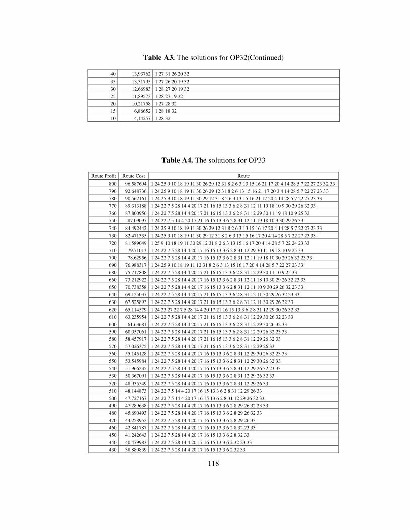
118


40 13,93762 1 27 31 26 20 32

35 13,31795 1 27 26 20 19 32

30 12,66983 1 28 27 20 19 32

25 11,89573 1 28 27 19 32

20 10,21758 1 27 28 32

15 6,86652 1 28 18 32

10 4,14257 1 28 32



800 96.587694 1 24 25 9 10 18 19 11 30 26 29 12 31 8 2 6 3 13 15 16 21 17 20 4 14 28 5 7 22 27 23 32 33

790 92.648736 1 24 25 9 10 18 19 11 30 26 29 12 31 8 2 6 13 15 16 21 17 20 3 4 14 28 5 7 22 27 23 33

780 90.562161 1 24 25 9 10 18 19 11 30 29 12 31 8 2 6 3 13 15 16 21 17 20 4 14 28 5 7 22 27 23 33

770 89.313188 1 24 22 7 5 28 14 4 20 17 21 16 15 13 3 6 2 8 31 12 11 19 18 10 9 30 29 26 32 33

760 87.800956 1 24 22 7 5 28 14 4 20 17 21 16 15 13 3 6 2 8 31 12 29 30 11 19 18 10 9 25 33

750 87.09097 1 24 22 7 5 14 4 20 17 21 16 15 13 3 6 2 8 31 12 11 19 18 10 9 30 29 26 33

740 84.492442 1 24 25 9 10 18 19 11 30 26 29 12 31 8 2 6 3 13 15 16 17 20 4 14 28 5 7 22 27 23 33

730 82.471335 1 24 25 9 10 18 19 11 30 29 12 31 8 2 6 3 13 15 16 17 20 4 14 28 5 7 22 27 23 33

720 81.589049 1 25 9 10 18 19 11 30 29 12 31 8 2 6 3 13 15 16 17 20 4 14 28 5 7 22 24 23 33

710 79.71013 1 24 22 7 5 28 14 4 20 17 16 15 13 3 6 2 8 31 12 29 30 11 19 18 10 9 25 33

700 78.62956 1 24 22 7 5 28 14 4 20 17 16 15 13 3 6 2 8 31 12 11 19 18 10 30 29 26 32 23 33

690 76.988317 1 24 25 9 10 18 19 11 12 31 8 2 6 3 13 15 16 17 20 4 14 28 5 7 22 27 23 33

680 75.717808 1 24 22 7 5 28 14 4 20 17 21 16 15 13 3 6 2 8 31 12 29 30 11 10 9 25 33

660 73.212922 1 24 22 7 5 28 14 4 20 17 16 15 13 3 6 2 8 31 12 11 18 10 30 29 26 32 23 33

650 70.738358 1 24 22 7 5 28 14 4 20 17 16 15 13 3 6 2 8 31 12 11 10 9 30 29 26 32 23 33

640 69.125037 1 24 22 7 5 28 14 4 20 17 21 16 15 13 3 6 2 8 31 12 11 30 29 26 32 23 33

630 67.525893 1 24 22 7 5 28 14 4 20 17 21 16 15 13 3 6 2 8 31 12 11 30 29 26 32 33

620 65.114579 1 24 23 27 22 7 5 28 14 4 20 17 21 16 15 13 3 6 2 8 31 12 29 30 26 32 33

610 63.235954 1 24 22 7 5 28 14 4 20 17 21 16 15 13 3 6 2 8 31 12 29 30 26 32 23 33

600 61.63681 1 24 22 7 5 28 14 4 20 17 21 16 15 13 3 6 2 8 31 12 29 30 26 32 33

590 60.057061 1 24 22 7 5 28 14 4 20 17 21 16 15 13 3 6 2 8 31 12 29 26 32 23 33

580 58.457917 1 24 22 7 5 28 14 4 20 17 21 16 15 13 3 6 2 8 31 12 29 26 32 33

570 57.026375 1 24 22 7 5 28 14 4 20 17 21 16 15 13 3 6 2 8 31 12 29 26 33

560 55.145128 1 24 22 7 5 28 14 4 20 17 16 15 13 3 6 2 8 31 12 29 30 26 32 23 33

550 53.545984 1 24 22 7 5 28 14 4 20 17 16 15 13 3 6 2 8 31 12 29 30 26 32 33

540 51.966235 1 24 22 7 5 28 14 4 20 17 16 15 13 3 6 2 8 31 12 29 26 32 23 33

530 50.367091 1 24 22 7 5 28 14 4 20 17 16 15 13 3 6 2 8 31 12 29 26 32 33

520 48.935549 1 24 22 7 5 28 14 4 20 17 16 15 13 3 6 2 8 31 12 29 26 33

510 48.144873 1 24 22 7 5 14 4 20 17 16 15 13 3 6 2 8 31 12 29 26 33

500 47.727167 1 24 22 7 5 14 4 20 17 16 15 13 6 2 8 31 12 29 26 32 33

490 47.289638 1 24 22 7 5 28 14 4 20 17 16 15 13 3 6 2 8 29 26 32 23 33

480 45.690493 1 24 22 7 5 28 14 4 20 17 16 15 13 3 6 2 8 29 26 32 33

470 44.258952 1 24 22 7 5 28 14 4 20 17 16 15 13 3 6 2 8 29 26 33

460 42.841787 1 24 22 7 5 28 14 4 20 17 16 15 13 3 6 2 8 32 23 33

450 41.242643 1 24 22 7 5 28 14 4 20 17 16 15 13 3 6 2 8 32 33

440 40.479983 1 24 22 7 5 28 14 4 20 17 16 15 13 3 6 2 32 23 33

430 38.880839 1 24 22 7 5 28 14 4 20 17 16 15 13 3 6 2 32 33

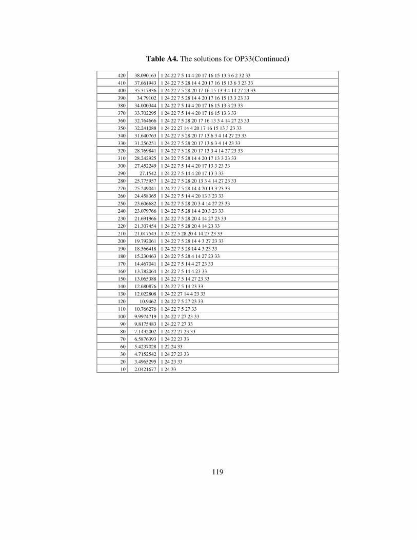
119


420 38.090163 1 24 22 7 5 14 4 20 17 16 15 13 3 6 2 32 33

410 37.661943 1 24 22 7 5 28 14 4 20 17 16 15 13 6 3 23 33

400 35.317936 1 24 22 7 5 28 20 17 16 15 13 3 4 14 27 23 33

390 34.79102 1 24 22 7 5 28 14 4 20 17 16 15 13 3 23 33

380 34.000344 1 24 22 7 5 14 4 20 17 16 15 13 3 23 33

370 33.702295 1 24 22 7 5 14 4 20 17 16 15 13 3 33

360 32.764666 1 24 22 7 5 28 20 17 16 13 3 4 14 27 23 33

350 32.241088 1 24 22 27 14 4 20 17 16 15 13 3 23 33

340 31.640763 1 24 22 7 5 28 20 17 13 6 3 4 14 27 23 33

330 31.256251 1 24 22 7 5 28 20 17 13 6 3 4 14 23 33

320 28.769841 1 24 22 7 5 28 20 17 13 3 4 14 27 23 33

310 28.242925 1 24 22 7 5 28 14 4 20 17 13 3 23 33

300 27.452249 1 24 22 7 5 14 4 20 17 13 3 23 33

290 27.1542 1 24 22 7 5 14 4 20 17 13 3 33

280 25.775957 1 24 22 7 5 28 20 13 3 4 14 27 23 33

270 25.249041 1 24 22 7 5 28 14 4 20 13 3 23 33

260 24.458365 1 24 22 7 5 14 4 20 13 3 23 33

250 23.606682 1 24 22 7 5 28 20 3 4 14 27 23 33

240 23.079766 1 24 22 7 5 28 14 4 20 3 23 33

230 21.691966 1 24 22 7 5 28 20 4 14 27 23 33

220 21.307454 1 24 22 7 5 28 20 4 14 23 33

210 21.017543 1 24 22 5 28 20 4 14 27 23 33

200 19.792061 1 24 22 7 5 28 14 4 3 27 23 33

190 18.566418 1 24 22 7 5 28 14 4 3 23 33

180 15.230463 1 24 22 7 5 28 4 14 27 23 33

170 14.467041 1 24 22 7 5 14 4 27 23 33

160 13.782064 1 24 22 7 5 14 4 23 33

150 13.065388 1 24 22 7 5 14 27 23 33

140 12.680876 1 24 22 7 5 14 23 33

130 12.022808 1 24 22 27 14 4 23 33

120 10.9462 1 24 22 7 5 27 23 33

110 10.766276 1 24 22 7 5 27 33

100 9.9974719 1 24 22 7 27 23 33

90 9.8175483 1 24 22 7 27 33

80 7.1432002 1 24 22 27 23 33

70 6.5876393 1 24 22 23 33

60 5.4237028 1 22 24 33

30 4.7152542 1 24 27 23 33

20 3.4965295 1 24 23 33

10 2.0421677 1 24 33

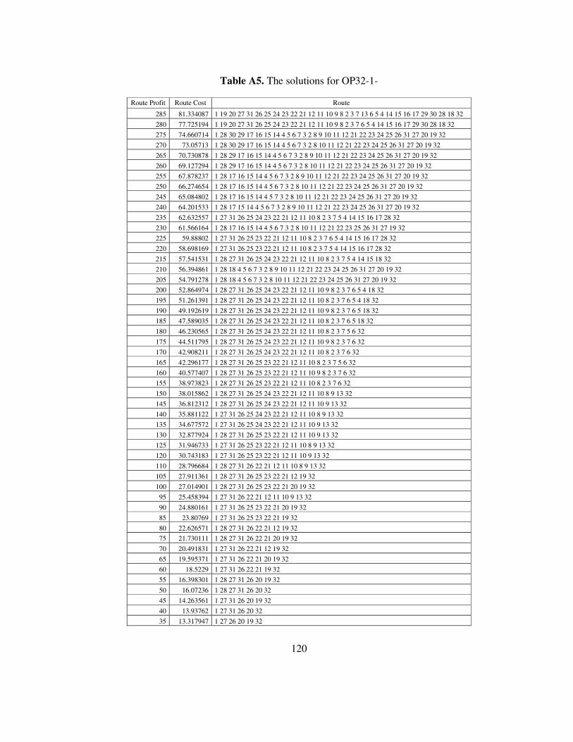
120

Table A5. The solutions for OP32-1-


285 81.334087 1 19 20 27 31 26 25 24 23 22 21 12 11 10 9 8 2 3 7 13 6 5 4 14 15 16 17 29 30 28 18 32

280 77.725194 1 19 20 27 31 26 25 24 23 22 21 12 11 10 9 8 2 3 7 6 5 4 14 15 16 17 29 30 28 18 32

275 74.660714 1 28 30 29 17 16 15 14 4 5 6 7 3 2 8 9 10 11 12 21 22 23 24 25 26 31 27 20 19 32

270 73.05713 1 28 30 29 17 16 15 14 4 5 6 7 3 2 8 10 11 12 21 22 23 24 25 26 31 27 20 19 32

265 70.730878 1 28 29 17 16 15 14 4 5 6 7 3 2 8 9 10 11 12 21 22 23 24 25 26 31 27 20 19 32

260 69.127294 1 28 29 17 16 15 14 4 5 6 7 3 2 8 10 11 12 21 22 23 24 25 26 31 27 20 19 32

255 67.878237 1 28 17 16 15 14 4 5 6 7 3 2 8 9 10 11 12 21 22 23 24 25 26 31 27 20 19 32

250 66.274654 1 28 17 16 15 14 4 5 6 7 3 2 8 10 11 12 21 22 23 24 25 26 31 27 20 19 32

245 65.084802 1 28 17 16 15 14 4 5 7 3 2 8 10 11 12 21 22 23 24 25 26 31 27 20 19 32

240 64.201533 1 28 17 15 14 4 5 6 7 3 2 8 9 10 11 12 21 22 23 24 25 26 31 27 20 19 32

235 62.632557 1 27 31 26 25 24 23 22 21 12 11 10 8 2 3 7 5 4 14 15 16 17 28 32

230 61.566164 1 28 17 16 15 14 4 5 6 7 3 2 8 10 11 12 21 22 23 25 26 31 27 19 32

225 59.88802 1 27 31 26 25 23 22 21 12 11 10 8 2 3 7 6 5 4 14 15 16 17 28 32

220 58.698169 1 27 31 26 25 23 22 21 12 11 10 8 2 3 7 5 4 14 15 16 17 28 32

215 57.541531 1 28 27 31 26 25 24 23 22 21 12 11 10 8 2 3 7 5 4 14 15 18 32

210 56.394861 1 28 18 4 5 6 7 3 2 8 9 10 11 12 21 22 23 24 25 26 31 27 20 19 32

205 54.791278 1 28 18 4 5 6 7 3 2 8 10 11 12 21 22 23 24 25 26 31 27 20 19 32

200 52.864974 1 28 27 31 26 25 24 23 22 21 12 11 10 9 8 2 3 7 6 5 4 18 32

195 51.261391 1 28 27 31 26 25 24 23 22 21 12 11 10 8 2 3 7 6 5 4 18 32

190 49.192619 1 28 27 31 26 25 24 23 22 21 12 11 10 9 8 2 3 7 6 5 18 32

185 47.589035 1 28 27 31 26 25 24 23 22 21 12 11 10 8 2 3 7 6 5 18 32

180 46.230565 1 28 27 31 26 25 24 23 22 21 12 11 10 8 2 3 7 5 6 32

175 44.511795 1 28 27 31 26 25 24 23 22 21 12 11 10 9 8 2 3 7 6 32

170 42.908211 1 28 27 31 26 25 24 23 22 21 12 11 10 8 2 3 7 6 32

165 42.296177 1 28 27 31 26 25 23 22 21 12 11 10 8 2 3 7 5 6 32

160 40.577407 1 28 27 31 26 25 23 22 21 12 11 10 9 8 2 3 7 6 32

155 38.973823 1 28 27 31 26 25 23 22 21 12 11 10 8 2 3 7 6 32

150 38.015862 1 28 27 31 26 25 24 23 22 21 12 11 10 8 9 13 32

145 36.812312 1 28 27 31 26 25 24 23 22 21 12 11 10 9 13 32

140 35.881122 1 27 31 26 25 24 23 22 21 12 11 10 8 9 13 32

135 34.677572 1 27 31 26 25 24 23 22 21 12 11 10 9 13 32

130 32.877924 1 28 27 31 26 25 23 22 21 12 11 10 9 13 32

125 31.946733 1 27 31 26 25 23 22 21 12 11 10 8 9 13 32

120 30.743183 1 27 31 26 25 23 22 21 12 11 10 9 13 32

110 28.796684 1 28 27 31 26 22 21 12 11 10 8 9 13 32

105 27.911361 1 28 27 31 26 25 23 22 21 12 19 32

100 27.014901 1 28 27 31 26 25 23 22 21 20 19 32

95 25.458394 1 27 31 26 22 21 12 11 10 9 13 32

90 24.880161 1 27 31 26 25 23 22 21 20 19 32

85 23.80769 1 27 31 26 25 23 22 21 19 32

80 22.626571 1 28 27 31 26 22 21 12 19 32

75 21.730111 1 28 27 31 26 22 21 20 19 32

70 20.491831 1 27 31 26 22 21 12 19 32

65 19.595371 1 27 31 26 22 21 20 19 32

60 18.5229 1 27 31 26 22 21 19 32

55 16.398301 1 28 27 31 26 20 19 32

50 16.07236 1 28 27 31 26 20 32

45 14.263561 1 27 31 26 20 19 32

40 13.93762 1 27 31 26 20 32

35 13.317947 1 27 26 20 19 32

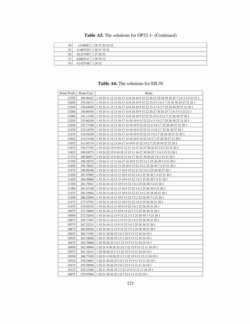
121

Table A5. The solutions for OP32-1- (Continued)

30 12.66983 1 28 27 20 19 32

25 11.895729 1 28 27 19 32

20 10.217585 1 27 28 32

15 6.8665211 1 28 18 32

10 4.1425748 1 28 32

Table A6. The solutions for EIL30


12750 385.86423 1 19 24 11 12 13 16 17 14 8 18 10 9 15 22 20 27 29 28 30 26 25 7 2 6 3 5 4 23 21 1

12650 376.28171 1 19 24 11 12 13 16 17 14 8 18 10 9 15 22 23 4 5 3 6 2 7 25 26 30 29 27 21 20 1

12550 370.45049 1 19 24 11 12 13 16 17 14 8 18 10 9 15 22 23 4 3 6 2 7 25 26 30 29 27 21 20 1

12500 350.08104 1 19 24 11 12 13 16 17 14 8 18 10 9 15 22 20 27 30 26 25 7 2 6 3 5 4 23 21 1

12400 341.11548 1 19 24 11 12 13 16 17 14 8 18 10 9 15 22 21 23 4 3 6 2 7 25 26 30 27 20 1

12350 333.60228 1 19 24 11 12 13 16 17 14 18 10 9 15 22 23 4 5 3 6 2 7 25 26 30 27 21 20 1

12250 327.77106 1 19 24 11 12 13 16 17 14 18 10 9 15 22 23 4 3 6 2 7 25 26 30 27 21 20 1

12150 322.41079 1 19 24 11 12 13 16 17 14 18 10 9 15 22 21 4 3 6 2 7 25 26 30 27 20 1

12125 318.59429 1 19 24 11 12 13 16 17 14 18 10 9 15 22 23 3 6 2 7 25 26 30 27 21 20 1

12025 314.51346 1 19 24 11 12 13 16 17 14 18 10 9 15 22 3 6 2 7 25 26 30 27 21 20 1

11925 311.65174 1 19 24 11 12 13 16 17 14 10 9 15 22 3 6 2 7 25 26 30 27 21 20 1

11875 310.77783 1 19 24 22 15 9 10 13 12 11 14 17 16 27 30 26 25 2 6 3 23 21 20 1

11825 309.54573 1 19 24 22 15 9 10 18 13 12 11 16 27 30 26 25 7 2 6 3 23 21 20 1

11775 305.66071 1 19 24 22 15 9 10 13 12 14 17 16 27 30 26 25 2 6 3 23 21 20 1

11750 298.38275 1 19 24 11 12 13 16 17 14 10 9 15 22 3 6 2 25 26 30 7 4 21 20 1

11650 294.79622 1 19 24 11 16 12 13 18 10 9 15 22 3 6 2 25 26 30 7 4 23 21 20 1

11575 290.98106 1 19 24 11 16 12 13 10 9 15 22 21 23 3 6 2 25 26 30 27 20 1

11550 287.97805 1 19 24 11 16 12 13 10 9 15 22 3 6 2 25 26 30 7 4 23 21 20 1

11450 284.30868 1 19 24 11 16 12 13 10 9 15 22 3 6 2 25 26 30 7 4 21 20 1

11350 281.75621 1 19 24 16 12 13 10 9 15 22 3 6 2 25 26 30 7 4 21 20 1

11300 281.67188 1 19 24 11 16 12 13 10 9 15 22 3 6 2 25 26 30 4 21 20 1

11275 281.55864 1 19 24 11 16 12 13 10 9 15 22 23 3 6 2 25 26 30 21 20 1

11250 280.22956 1 19 24 16 12 13 10 9 15 22 3 5 2 25 26 30 7 4 21 20 1

11175 277.47781 1 19 24 11 16 12 13 10 9 15 22 3 6 2 25 26 30 21 20 1

11075 274.92534 1 19 24 16 12 13 10 9 15 22 3 6 2 25 26 30 21 20 1

10975 273.39869 1 19 24 16 12 13 10 9 15 22 3 5 2 25 26 30 21 20 1

10950 272.52643 1 19 24 16 12 13 9 15 22 3 5 2 25 26 30 7 4 21 20 1

10875 269.77467 1 19 24 11 16 12 13 9 15 22 3 6 2 25 26 30 21 20 1

10775 267.22221 1 19 24 16 12 13 9 15 22 3 6 2 25 26 30 21 20 1

10675 265.69556 1 19 24 16 12 13 9 15 22 3 5 2 25 26 30 21 20 1

10625 264.71492 1 20 21 30 26 25 2 6 3 22 9 13 12 16 24 19 1

10525 263.18828 1 20 21 30 26 25 2 5 3 22 9 13 12 16 24 19 1

10475 262.70806 1 20 30 26 25 2 6 3 22 15 9 13 12 16 24 19 1

10450 262.30094 1 20 21 4 30 26 25 2 6 3 22 15 9 13 12 11 24 19 1

10375 261.18141 1 20 30 26 25 2 5 3 22 15 9 13 12 16 24 19 1

10350 260.77429 1 20 21 4 30 26 25 2 5 3 22 15 9 13 12 11 24 19 1

10325 258.10687 1 20 21 30 26 25 2 6 3 22 15 9 13 12 11 24 19 1

10175 255.59958 1 20 21 30 26 25 2 6 3 22 9 13 12 11 24 19 1

10125 255.27405 1 20 21 30 26 25 2 3 22 15 9 13 12 11 24 19 1

10075 255.07084 1 20 21 30 26 25 2 6 3 22 9 13 12 24 19 1

122

Table A6. The solutions for EIL30 (Continued)

9975 252.76676 1 20 21 30 26 25 2 3 22 9 13 12 11 24 19 1

9875 251.08543 1 20 30 26 25 2 6 3 22 9 13 12 11 24 19 1

9825 250.7599 1 20 30 26 25 2 3 22 15 9 13 12 11 24 19 1

9775 249.55879 1 20 30 26 25 2 5 3 22 9 13 12 11 24 19 1

9675 248.25262 1 20 30 26 25 2 3 22 9 13 12 11 24 19 1

9225 236.76308 1 19 24 22 21 23 4 3 6 2 7 25 26 30 27 20 1

9200 234.93793 1 20 27 30 26 25 2 7 5 6 3 23 21 22 24 19 1

9100 227.58631 1 20 27 30 26 25 7 2 6 3 23 21 22 24 19 1

9025 225.33986 1 20 21 23 4 5 7 30 26 25 2 6 3 22 24 19 1

9000 225.07311 1 20 27 30 26 25 2 7 5 3 23 21 22 24 19 1

8975 224.10715 1 20 27 30 26 25 2 6 3 4 21 22 24 19 1

8950 218.59976 1 20 27 30 26 25 2 6 3 23 21 22 24 19 1

8925 215.59675 1 20 21 23 4 7 30 26 25 2 6 3 22 24 19 1

8825 211.92738 1 20 21 4 7 30 26 25 2 6 3 22 24 19 1

8700 210.87012 1 20 21 7 30 26 25 2 6 3 22 24 19 1

8675 209.29058 1 20 21 4 30 26 25 2 6 3 22 24 19 1

8650 209.17734 1 19 24 22 23 3 6 2 25 26 30 21 20 1

8625 209.09456 1 19 24 22 3 2 25 26 30 7 4 21 20 1

8575 207.76394 1 19 24 22 3 5 2 25 26 30 4 21 20 1

8550 205.09651 1 19 24 22 3 6 2 25 26 30 21 20 1

8450 203.56986 1 19 24 22 3 5 2 25 26 30 21 20 1

8350 202.26369 1 19 24 22 3 2 25 26 30 21 20 1

8250 200.58236 1 20 30 26 25 2 6 3 22 24 19 1

8150 199.05572 1 20 30 26 25 2 5 3 22 24 19 1

8100 197.25523 1 20 21 30 26 25 2 6 3 22 1

8000 195.72858 1 20 21 30 26 25 2 5 3 22 1

7900 194.42241 1 22 3 2 25 26 30 21 20 1

7800 192.74108 1 22 3 6 2 25 26 30 20 1

7700 191.21443 1 22 3 5 2 25 26 30 20 1

7600 189.90826 1 22 3 2 25 26 30 20 1

7300 189.43731 1 22 3 25 26 30 20 1

7275 188.89561 1 20 27 30 26 25 7 2 6 3 4 23 21 1

7250 187.07046 1 20 27 30 26 25 2 7 5 6 3 23 21 1

7225 185.74028 1 20 27 30 26 25 2 6 3 5 4 23 21 1

7175 185.22623 1 21 4 3 6 2 7 25 26 30 27 20 1

7150 179.71884 1 20 27 30 26 25 7 2 6 3 23 21 1

7100 179.07046 1 20 27 30 26 25 2 5 6 3 23 21 1

7025 176.23968 1 20 27 30 26 25 2 6 3 4 21 1

7000 170.73229 1 20 27 30 26 25 2 6 3 23 21 1

6900 169.20564 1 20 27 30 26 25 2 5 3 23 21 1

6800 167.89947 1 20 27 30 26 25 2 3 23 21 1

6750 167.7487 1 20 7 30 26 25 2 5 3 23 21 1

6725 167.21311 1 20 4 30 26 25 2 5 3 23 21 1

6700 162.19607 1 21 23 3 6 2 25 26 30 20 1

6600 160.66943 1 20 30 26 25 2 5 3 23 21 1

6500 159.36326 1 20 30 26 25 2 3 23 21 1

6400 158.85519 1 20 30 26 25 2 3 21 1

5850 156.12363 1 19 24 22 3 23 21 20 1

5750 155.61556 1 19 24 22 3 21 20 1

5700 155.58107 1 24 22 3 23 21 20 1

5600 155.073 1 20 21 3 22 24 1

5450 153.45495 1 21 23 3 22 24 19 1

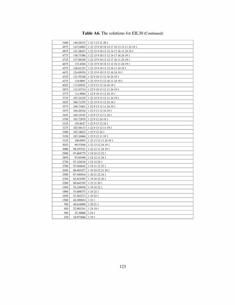
123


5400 148.28235 1 22 3 23 21 20 1

4975 143.54802 1 22 15 9 10 18 14 17 16 13 12 11 24 19 1

4875 141.28633 1 22 15 9 10 13 12 14 17 16 11 24 19 1

4775 138.73386 1 22 15 9 10 13 12 14 17 16 24 19 1

4725 137.08109 1 22 15 9 10 13 12 17 16 11 24 19 1

4675 133.4304 1 22 15 9 10 18 13 12 16 11 24 19 1

4575 126.61223 1 22 15 9 10 13 12 16 11 24 19 1

4475 124.05976 1 22 15 9 10 13 12 16 24 19 1

4325 121.55248 1 22 9 10 13 12 16 24 19 1

4275 118.9091 1 22 15 9 13 12 16 11 24 19 1

4025 113.84935 1 22 9 13 12 16 24 19 1

3875 112.43714 1 22 9 10 13 12 11 24 19 1

3775 111.9084 1 22 9 10 13 12 24 19 1

3725 107.24129 1 22 15 9 13 12 11 24 19 1

3625 106.71255 1 22 15 9 13 12 24 19 1

3575 104.73401 1 22 9 13 12 11 24 19 1

3475 104.20526 1 22 9 13 12 24 19 1

3425 104.19145 1 22 9 13 12 11 24 1

3350 103.72879 1 22 9 12 24 19 1

3325 103.6627 1 22 9 13 12 24 1

3275 103.58113 1 22 9 13 12 11 19 1

3200 103.18623 1 22 9 12 24 1

3150 103.10466 1 22 9 12 11 19 1

3125 100.0993 1 22 13 12 11 24 19 1

3025 99.57056 1 22 13 12 24 19 1

3000 98.197521 1 22 12 11 24 19 1

2900 97.668779 1 19 24 12 22 1

2850 97.65496 1 22 12 11 24 1

2750 97.126218 1 22 12 24 1

2700 97.044642 1 19 11 12 22 1

2650 88.483477 1 19 24 22 21 20 1

2500 87.940916 1 20 21 22 24 1

2350 82.624585 1 19 24 22 20 1

2200 80.642195 1 22 21 20 1

1950 54.230936 1 19 24 22 1

1800 53.688375 1 24 22 1

1650 53.562273 1 19 22 1

1500 46.389654 1 22 1

700 40.616006 1 20 21 1

450 22.903241 1 24 19 1

300 22.36068 1 24 1

150 18.973666 1 19 1

124



29370 448.10668 1 31 32 2 14 15 16 18 26 27 28 29 30 17 25 24 23 21 22 20 19 11 10 9 8 7 6 33 12 13 3 4 5 1

29330 444.25998 1 31 32 2 14 15 16 18 26 27 28 29 30 17 25 24 23 21 22 20 19 11 10 9 8 7 33 12 13 3 4 5 1

29120 437.38696 1 31 32 2 15 16 18 26 27 28 29 30 17 25 24 23 21 22 20 19 11 10 9 8 7 6 33 12 13 3 4 5 1

29080 433.54027 1 31 32 2 15 16 18 26 27 28 29 30 17 25 24 23 21 22 20 19 11 10 9 8 7 33 12 13 3 4 5 1

28870 422.91531 1 31 32 2 14 15 16 18 26 27 28 29 17 25 24 23 21 22 20 19 11 10 9 8 7 6 33 12 13 3 4 5 1

28830 419.06862 1 31 32 2 14 15 16 18 26 27 28 29 17 25 24 23 21 22 20 19 11 10 9 8 7 33 12 13 3 4 5 1

28670 417.69627 1 31 32 2 14 15 16 18 26 27 30 29 28 25 24 23 21 22 20 19 11 10 9 8 7 6 33 12 13 3 4 5 1

28630 413.84957 1 31 32 2 14 15 16 18 26 27 30 29 28 25 24 23 21 22 20 19 11 10 9 8 7 33 12 13 3 4 5 1

28620 412.1956 1 31 32 2 15 16 18 26 27 28 29 17 25 24 23 21 22 20 19 11 10 9 8 7 6 33 12 13 3 4 5 1

28420 406.97655 1 31 32 2 15 16 18 26 27 30 29 28 25 24 23 21 22 20 19 11 10 9 8 7 6 33 12 13 3 4 5 1

28380 403.12986 1 31 32 2 15 16 18 26 27 30 29 28 25 24 23 21 22 20 19 11 10 9 8 7 33 12 13 3 4 5 1

28180 398.58868 1 31 32 2 15 16 18 26 27 28 29 17 25 24 23 21 22 20 19 11 10 9 8 7 33 12 13 3 5 1

28170 395.31592 1 31 32 2 14 15 16 18 26 27 29 28 25 24 23 21 22 20 19 11 10 9 8 7 6 33 12 13 3 4 5 1

28130 391.46922 1 31 32 2 14 15 16 18 26 27 29 28 25 24 23 21 22 20 19 11 10 9 8 7 33 12 13 3 4 5 1

27920 384.5962 1 31 32 2 15 16 18 26 27 29 28 25 24 23 21 22 20 19 11 10 9 8 7 6 33 12 13 3 4 5 1

27880 380.74951 1 31 32 2 15 16 18 26 27 29 28 25 24 23 21 22 20 19 11 10 9 8 7 33 12 13 3 4 5 1

27680 379.5218 1 31 32 2 15 16 18 26 27 29 28 25 24 23 21 22 19 11 10 9 8 7 33 12 13 3 4 5 1

27670 378.00535 1 31 32 2 14 15 16 18 26 27 28 29 17 25 24 23 21 22 20 19 11 10 9 8 7 6 33 12 13 3 4 1

27630 374.15866 1 31 32 2 14 15 16 18 26 27 28 29 17 25 24 23 21 22 20 19 11 10 9 8 7 33 12 13 3 4 1

27480 370.98928 1 31 32 2 15 16 18 26 27 29 28 25 24 23 21 22 20 19 11 10 9 8 7 33 12 13 3 5 1

27430 370.58261 1 31 32 2 14 15 16 18 27 30 29 28 26 25 24 23 21 22 20 19 11 10 9 8 7 33 12 13 3 4 1

27420 367.90571 1 31 32 2 15 16 18 26 27 28 29 17 25 24 23 21 22 20 19 11 10 9 33 8 7 6 12 13 3 4 1

27220 363.70959 1 31 32 2 15 16 18 27 30 29 28 26 25 24 23 21 22 20 19 11 10 9 8 7 6 33 12 13 3 4 1

27180 359.8629 1 31 32 2 15 16 18 27 30 29 28 26 25 24 23 21 22 20 19 11 10 9 8 7 33 12 13 3 4 1

26980 358.63519 1 31 32 2 15 16 18 27 30 29 28 26 25 24 23 21 22 19 11 10 9 8 7 33 12 13 3 4 1

26970 352.04896 1 31 32 2 14 15 16 18 27 29 28 26 25 24 23 21 22 20 19 11 10 9 8 7 6 33 12 13 3 4 1

26930 346.55926 1 31 32 2 14 15 16 18 26 27 29 28 25 24 23 21 22 20 19 11 10 9 8 7 33 12 13 3 4 1

26720 341.32924 1 31 32 2 15 16 18 27 29 28 26 25 24 23 21 22 20 19 11 10 9 8 7 6 33 12 13 3 4 1

26680 335.83955 1 31 32 2 15 16 18 26 27 29 28 25 24 23 21 22 20 19 11 10 9 8 7 33 12 13 3 4 1

26600 335.36741 1 31 32 2 15 16 18 26 27 29 28 25 24 23 21 22 20 19 11 10 9 8 33 12 13 3 4 1

26480 334.61184 1 31 32 2 15 16 18 26 27 29 28 25 24 23 21 22 19 11 10 9 8 7 33 12 13 3 4 1

26420 333.28922 1 31 32 2 15 16 18 26 27 29 28 25 24 21 23 20 19 11 10 9 8 7 6 33 12 13 3 4 1

26380 331.08552 1 31 32 2 15 16 18 27 29 28 26 25 24 21 23 20 19 11 10 9 8 7 33 12 13 3 4 1

26280 330.92903 1 31 32 2 15 16 18 27 29 28 26 25 24 23 22 20 19 11 10 9 8 7 33 12 13 3 4 1

26200 330.4569 1 31 32 2 15 16 18 27 29 28 26 25 24 23 22 20 19 11 10 9 8 33 12 13 3 4 1

26100 330.23758 1 31 32 2 15 16 18 27 29 28 26 25 24 21 23 19 11 10 9 8 33 12 13 3 4 1

26080 329.70133 1 31 32 2 15 16 18 27 29 28 26 25 24 23 22 19 11 10 9 8 7 33 12 13 3 4 1

26020 328.08332 1 31 32 2 15 16 18 27 29 28 26 25 24 23 20 19 11 10 9 8 7 6 33 12 13 3 4 1

26000 327.58619 1 31 32 2 15 16 18 26 27 29 28 25 24 23 22 19 11 10 9 8 33 12 13 3 4 1

25980 322.59363 1 4 3 13 12 33 7 8 9 10 11 19 20 23 24 25 28 29 27 26 18 16 15 2 32 31 1

25580 319.02646 1 31 32 2 15 16 18 26 27 29 28 25 23 22 20 19 11 10 9 8 7 33 12 13 3 4 1

25380 317.79875 1 31 32 2 15 16 18 26 27 29 28 25 23 22 19 11 10 9 8 7 33 12 13 3 4 1

25320 316.18075 1 4 3 13 12 33 6 7 8 9 10 11 19 20 23 25 28 29 27 26 18 16 15 2 32 31 1

25280 312.33405 1 4 3 13 12 33 7 8 9 10 11 19 20 23 25 28 29 27 26 18 16 15 2 32 31 1

25230 310.28629 1 4 3 13 12 33 7 8 9 10 11 19 20 22 21 23 26 28 29 27 18 16 15 2 32 31 1

25150 309.81415 1 4 3 13 12 33 8 9 10 11 19 20 22 21 23 26 28 29 27 18 16 15 2 32 31 1

25030 309.05858 1 4 3 13 12 33 7 8 9 10 11 19 22 21 23 26 28 29 27 18 16 15 2 32 31 1

24950 308.58645 1 4 3 13 12 33 8 9 10 11 19 22 21 23 26 28 29 27 18 16 15 2 32 31 1

24870 307.57947 1 4 3 13 12 33 6 7 8 9 10 11 19 20 22 23 26 28 29 27 18 16 15 2 32 31 1

24830 303.73277 1 4 3 13 12 33 7 8 9 10 11 19 20 22 23 26 28 29 27 18 16 15 2 32 31 1

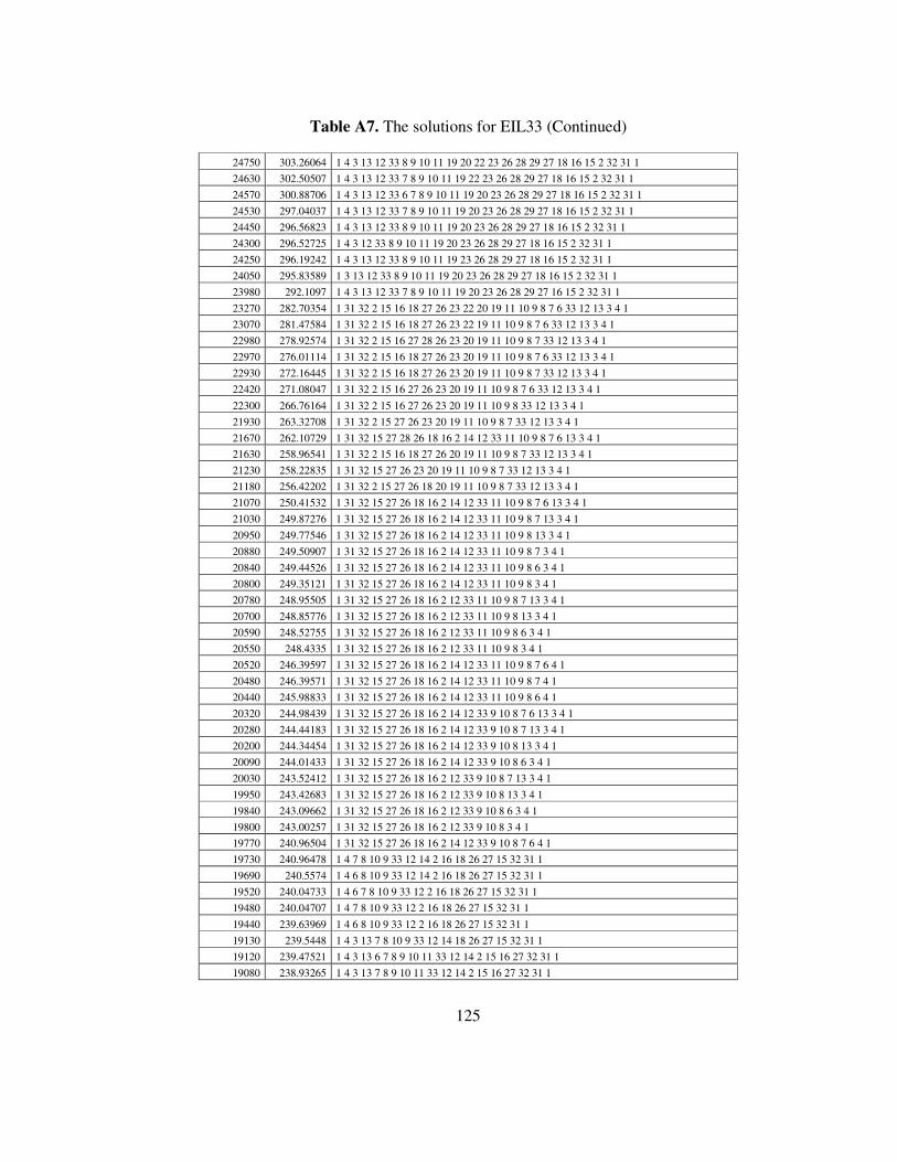
125


24750 303.26064 1 4 3 13 12 33 8 9 10 11 19 20 22 23 26 28 29 27 18 16 15 2 32 31 1

24630 302.50507 1 4 3 13 12 33 7 8 9 10 11 19 22 23 26 28 29 27 18 16 15 2 32 31 1

24570 300.88706 1 4 3 13 12 33 6 7 8 9 10 11 19 20 23 26 28 29 27 18 16 15 2 32 31 1

24530 297.04037 1 4 3 13 12 33 7 8 9 10 11 19 20 23 26 28 29 27 18 16 15 2 32 31 1

24450 296.56823 1 4 3 13 12 33 8 9 10 11 19 20 23 26 28 29 27 18 16 15 2 32 31 1

24300 296.52725 1 4 3 12 33 8 9 10 11 19 20 23 26 28 29 27 18 16 15 2 32 31 1

24250 296.19242 1 4 3 13 12 33 8 9 10 11 19 23 26 28 29 27 18 16 15 2 32 31 1

24050 295.83589 1 3 13 12 33 8 9 10 11 19 20 23 26 28 29 27 18 16 15 2 32 31 1

23980 292.1097 1 4 3 13 12 33 7 8 9 10 11 19 20 23 26 28 29 27 16 15 2 32 31 1

23270 282.70354 1 31 32 2 15 16 18 27 26 23 22 20 19 11 10 9 8 7 6 33 12 13 3 4 1

23070 281.47584 1 31 32 2 15 16 18 27 26 23 22 19 11 10 9 8 7 6 33 12 13 3 4 1

22980 278.92574 1 31 32 2 15 16 27 28 26 23 20 19 11 10 9 8 7 33 12 13 3 4 1

22970 276.01114 1 31 32 2 15 16 18 27 26 23 20 19 11 10 9 8 7 6 33 12 13 3 4 1

22930 272.16445 1 31 32 2 15 16 18 27 26 23 20 19 11 10 9 8 7 33 12 13 3 4 1

22420 271.08047 1 31 32 2 15 16 27 26 23 20 19 11 10 9 8 7 6 33 12 13 3 4 1

22300 266.76164 1 31 32 2 15 16 27 26 23 20 19 11 10 9 8 33 12 13 3 4 1

21930 263.32708 1 31 32 2 15 27 26 23 20 19 11 10 9 8 7 33 12 13 3 4 1

21670 262.10729 1 31 32 15 27 28 26 18 16 2 14 12 33 11 10 9 8 7 6 13 3 4 1

21630 258.96541 1 31 32 2 15 16 18 27 26 20 19 11 10 9 8 7 33 12 13 3 4 1

21230 258.22835 1 31 32 15 27 26 23 20 19 11 10 9 8 7 33 12 13 3 4 1

21180 256.42202 1 31 32 2 15 27 26 18 20 19 11 10 9 8 7 33 12 13 3 4 1

21070 250.41532 1 31 32 15 27 26 18 16 2 14 12 33 11 10 9 8 7 6 13 3 4 1

21030 249.87276 1 31 32 15 27 26 18 16 2 14 12 33 11 10 9 8 7 13 3 4 1

20950 249.77546 1 31 32 15 27 26 18 16 2 14 12 33 11 10 9 8 13 3 4 1

20880 249.50907 1 31 32 15 27 26 18 16 2 14 12 33 11 10 9 8 7 3 4 1

20840 249.44526 1 31 32 15 27 26 18 16 2 14 12 33 11 10 9 8 6 3 4 1

20800 249.35121 1 31 32 15 27 26 18 16 2 14 12 33 11 10 9 8 3 4 1

20780 248.95505 1 31 32 15 27 26 18 16 2 12 33 11 10 9 8 7 13 3 4 1

20700 248.85776 1 31 32 15 27 26 18 16 2 12 33 11 10 9 8 13 3 4 1

20590 248.52755 1 31 32 15 27 26 18 16 2 12 33 11 10 9 8 6 3 4 1

20550 248.4335 1 31 32 15 27 26 18 16 2 12 33 11 10 9 8 3 4 1

20520 246.39597 1 31 32 15 27 26 18 16 2 14 12 33 11 10 9 8 7 6 4 1

20480 246.39571 1 31 32 15 27 26 18 16 2 14 12 33 11 10 9 8 7 4 1

20440 245.98833 1 31 32 15 27 26 18 16 2 14 12 33 11 10 9 8 6 4 1

20320 244.98439 1 31 32 15 27 26 18 16 2 14 12 33 9 10 8 7 6 13 3 4 1

20280 244.44183 1 31 32 15 27 26 18 16 2 14 12 33 9 10 8 7 13 3 4 1

20200 244.34454 1 31 32 15 27 26 18 16 2 14 12 33 9 10 8 13 3 4 1

20090 244.01433 1 31 32 15 27 26 18 16 2 14 12 33 9 10 8 6 3 4 1

20030 243.52412 1 31 32 15 27 26 18 16 2 12 33 9 10 8 7 13 3 4 1

19950 243.42683 1 31 32 15 27 26 18 16 2 12 33 9 10 8 13 3 4 1

19840 243.09662 1 31 32 15 27 26 18 16 2 12 33 9 10 8 6 3 4 1

19800 243.00257 1 31 32 15 27 26 18 16 2 12 33 9 10 8 3 4 1

19770 240.96504 1 31 32 15 27 26 18 16 2 14 12 33 9 10 8 7 6 4 1

19730 240.96478 1 4 7 8 10 9 33 12 14 2 16 18 26 27 15 32 31 1

19690 240.5574 1 4 6 8 10 9 33 12 14 2 16 18 26 27 15 32 31 1

19520 240.04733 1 4 6 7 8 10 9 33 12 2 16 18 26 27 15 32 31 1

19480 240.04707 1 4 7 8 10 9 33 12 2 16 18 26 27 15 32 31 1

19440 239.63969 1 4 6 8 10 9 33 12 2 16 18 26 27 15 32 31 1

19130 239.5448 1 4 3 13 7 8 10 9 33 12 14 18 26 27 15 32 31 1

19120 239.47521 1 4 3 13 6 7 8 9 10 11 33 12 14 2 15 16 27 32 31 1

19080 238.93265 1 4 3 13 7 8 9 10 11 33 12 14 2 15 16 27 32 31 1

126


19070 237.78709 1 4 6 7 8 10 9 33 12 14 16 18 26 27 15 32 31 1

18670 235.56852 1 4 3 13 6 7 8 9 10 11 33 12 14 2 15 27 32 31 1

18570 235.13019 1 4 6 7 8 9 10 11 33 12 14 2 16 27 15 32 31 1

18370 233.71862 1 4 3 13 6 7 8 10 9 33 12 14 2 16 27 15 32 31 1

18330 233.17606 1 4 3 13 7 8 10 9 33 12 14 2 16 27 15 32 31 1

18140 232.74856 1 4 3 6 8 10 9 33 12 14 2 16 27 15 32 31 1

18120 231.54917 1 4 6 7 8 9 10 11 33 12 14 2 15 27 32 31 1

18080 231.54891 1 4 7 8 9 10 11 33 12 14 2 15 27 32 31 1

18040 231.14153 1 4 6 8 9 10 11 33 12 14 2 15 27 32 31 1

17920 230.13759 1 4 3 13 6 7 8 10 9 33 12 14 2 15 27 32 31 1

17880 229.59503 1 4 3 13 7 8 10 9 33 12 14 2 15 27 32 31 1

17800 229.49774 1 4 3 13 8 10 9 33 12 14 2 15 27 32 31 1

17690 229.16753 1 4 3 6 8 10 9 33 12 14 2 15 27 32 31 1

17630 228.67733 1 4 3 13 7 8 10 9 33 12 2 15 27 32 31 1

17550 228.58003 1 4 3 13 8 10 9 33 12 2 15 27 32 31 1

17490 228.37392 1 4 6 8 10 9 33 12 2 16 27 15 32 31 1

17480 228.31364 1 4 3 7 8 10 9 33 12 2 15 27 32 31 1

17440 228.24983 1 4 3 6 8 10 9 33 12 2 15 27 32 31 1

17400 228.15577 1 4 3 8 10 9 33 12 2 15 27 32 31 1

17370 226.11824 1 4 6 7 8 10 9 33 12 14 2 15 27 32 31 1

17330 226.11798 1 4 7 8 10 9 33 12 14 2 15 27 32 31 1

17290 225.7106 1 4 6 8 10 9 33 12 14 2 15 27 32 31 1

17120 225.20053 1 4 6 7 8 10 9 33 12 2 15 27 32 31 1

16770 224.76921 1 4 6 7 8 9 33 12 14 2 15 27 32 31 1

16730 224.76895 1 4 7 8 9 33 12 14 2 15 27 32 31 1

16690 224.36157 1 4 6 8 9 33 12 14 2 15 27 32 31 1

16630 224.25261 1 4 3 13 7 8 10 9 33 12 14 2 15 16 27 31 1

16550 224.15532 1 4 3 13 8 10 9 33 12 14 2 15 16 27 31 1

16520 223.8515 1 4 6 7 8 9 33 12 2 15 27 32 31 1

16480 223.85124 1 4 7 8 9 33 12 2 15 27 32 31 1

16440 223.44386 1 4 6 8 9 33 12 2 15 27 32 31 1

16420 222.30006 1 31 27 15 2 14 12 33 11 10 9 8 7 6 4 1

16380 222.2998 1 4 7 8 9 10 11 33 12 14 2 15 27 31 1

16340 221.89242 1 4 6 8 9 10 11 33 12 14 2 15 27 31 1

16180 220.34592 1 4 3 13 7 8 10 9 33 12 14 2 15 27 31 1

16070 220.32606 1 4 3 6 7 8 10 9 33 12 14 2 15 27 31 1

15990 219.91842 1 4 3 6 8 10 9 33 12 14 2 15 27 31 1

15930 219.42822 1 4 3 13 7 8 10 9 33 12 2 15 27 31 1

15670 216.86913 1 4 6 7 8 10 9 33 12 14 2 15 27 31 1

15120 207.67262 1 31 32 15 16 2 14 12 33 11 10 9 8 7 6 13 3 4 1

15080 207.13006 1 31 32 15 16 2 14 12 33 11 10 9 8 7 13 3 4 1

14670 202.02069 1 4 3 13 6 7 8 9 10 11 33 12 14 2 15 32 31 1

14630 201.47813 1 4 3 13 7 8 9 10 11 33 12 14 2 15 32 31 1

14550 201.38083 1 4 3 13 8 9 10 11 33 12 14 2 15 32 31 1

14440 201.05063 1 4 3 6 8 9 10 11 33 12 14 2 15 32 31 1

14400 200.95657 1 4 3 8 9 10 11 33 12 14 2 15 32 31 1

14380 200.56042 1 4 3 13 7 8 9 10 11 33 12 2 15 32 31 1

14300 200.46313 1 4 3 13 8 9 10 11 33 12 2 15 32 31 1

14190 200.13292 1 4 3 6 8 9 10 11 33 12 2 15 32 31 1

14150 200.03887 1 4 3 8 9 10 11 33 12 2 15 32 31 1

14120 198.00134 1 4 6 7 8 9 10 11 33 12 14 2 15 32 31 1

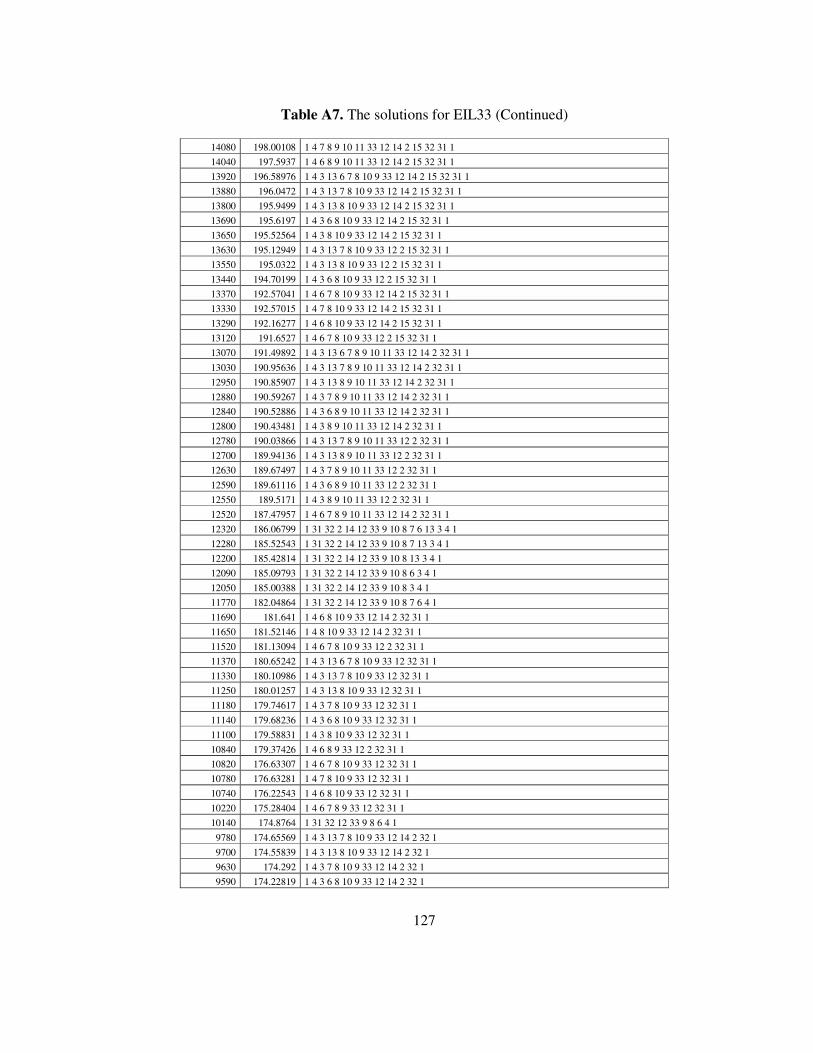
127


14080 198.00108 1 4 7 8 9 10 11 33 12 14 2 15 32 31 1

14040 197.5937 1 4 6 8 9 10 11 33 12 14 2 15 32 31 1

13920 196.58976 1 4 3 13 6 7 8 10 9 33 12 14 2 15 32 31 1

13880 196.0472 1 4 3 13 7 8 10 9 33 12 14 2 15 32 31 1

13800 195.9499 1 4 3 13 8 10 9 33 12 14 2 15 32 31 1

13690 195.6197 1 4 3 6 8 10 9 33 12 14 2 15 32 31 1

13650 195.52564 1 4 3 8 10 9 33 12 14 2 15 32 31 1

13630 195.12949 1 4 3 13 7 8 10 9 33 12 2 15 32 31 1

13550 195.0322 1 4 3 13 8 10 9 33 12 2 15 32 31 1

13440 194.70199 1 4 3 6 8 10 9 33 12 2 15 32 31 1

13370 192.57041 1 4 6 7 8 10 9 33 12 14 2 15 32 31 1

13330 192.57015 1 4 7 8 10 9 33 12 14 2 15 32 31 1

13290 192.16277 1 4 6 8 10 9 33 12 14 2 15 32 31 1

13120 191.6527 1 4 6 7 8 10 9 33 12 2 15 32 31 1

13070 191.49892 1 4 3 13 6 7 8 9 10 11 33 12 14 2 32 31 1

13030 190.95636 1 4 3 13 7 8 9 10 11 33 12 14 2 32 31 1

12950 190.85907 1 4 3 13 8 9 10 11 33 12 14 2 32 31 1

12880 190.59267 1 4 3 7 8 9 10 11 33 12 14 2 32 31 1

12840 190.52886 1 4 3 6 8 9 10 11 33 12 14 2 32 31 1

12800 190.43481 1 4 3 8 9 10 11 33 12 14 2 32 31 1

12780 190.03866 1 4 3 13 7 8 9 10 11 33 12 2 32 31 1

12700 189.94136 1 4 3 13 8 9 10 11 33 12 2 32 31 1

12630 189.67497 1 4 3 7 8 9 10 11 33 12 2 32 31 1

12590 189.61116 1 4 3 6 8 9 10 11 33 12 2 32 31 1

12550 189.5171 1 4 3 8 9 10 11 33 12 2 32 31 1

12520 187.47957 1 4 6 7 8 9 10 11 33 12 14 2 32 31 1

12320 186.06799 1 31 32 2 14 12 33 9 10 8 7 6 13 3 4 1

12280 185.52543 1 31 32 2 14 12 33 9 10 8 7 13 3 4 1

12200 185.42814 1 31 32 2 14 12 33 9 10 8 13 3 4 1

12090 185.09793 1 31 32 2 14 12 33 9 10 8 6 3 4 1

12050 185.00388 1 31 32 2 14 12 33 9 10 8 3 4 1

11770 182.04864 1 31 32 2 14 12 33 9 10 8 7 6 4 1

11690 181.641 1 4 6 8 10 9 33 12 14 2 32 31 1

11650 181.52146 1 4 8 10 9 33 12 14 2 32 31 1

11520 181.13094 1 4 6 7 8 10 9 33 12 2 32 31 1

11370 180.65242 1 4 3 13 6 7 8 10 9 33 12 32 31 1

11330 180.10986 1 4 3 13 7 8 10 9 33 12 32 31 1

11250 180.01257 1 4 3 13 8 10 9 33 12 32 31 1

11180 179.74617 1 4 3 7 8 10 9 33 12 32 31 1

11140 179.68236 1 4 3 6 8 10 9 33 12 32 31 1

11100 179.58831 1 4 3 8 10 9 33 12 32 31 1

10840 179.37426 1 4 6 8 9 33 12 2 32 31 1

10820 176.63307 1 4 6 7 8 10 9 33 12 32 31 1

10780 176.63281 1 4 7 8 10 9 33 12 32 31 1

10740 176.22543 1 4 6 8 10 9 33 12 32 31 1

10220 175.28404 1 4 6 7 8 9 33 12 32 31 1

10140 174.8764 1 31 32 12 33 9 8 6 4 1

9780 174.65569 1 4 3 13 7 8 10 9 33 12 14 2 32 1

9700 174.55839 1 4 3 13 8 10 9 33 12 14 2 32 1

9630 174.292 1 4 3 7 8 10 9 33 12 14 2 32 1

9590 174.22819 1 4 3 6 8 10 9 33 12 14 2 32 1

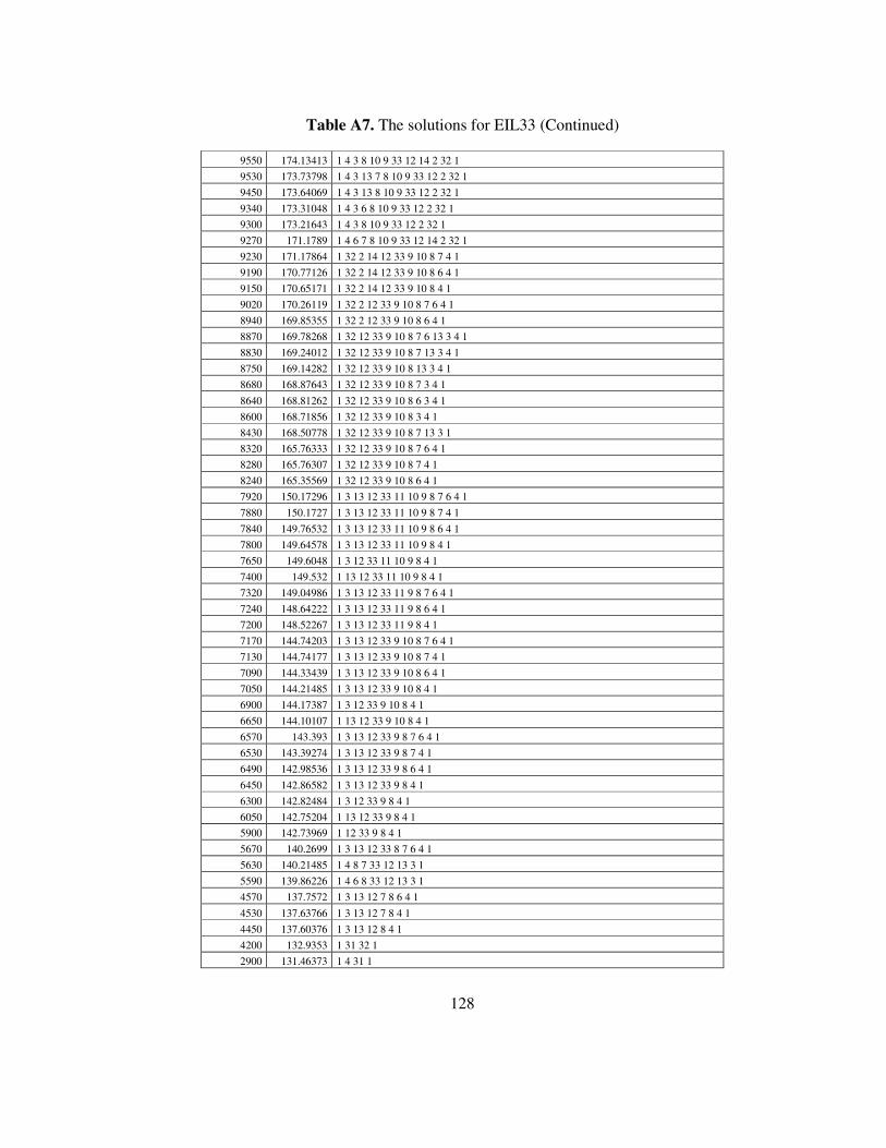
128


9550 174.13413 1 4 3 8 10 9 33 12 14 2 32 1

9530 173.73798 1 4 3 13 7 8 10 9 33 12 2 32 1

9450 173.64069 1 4 3 13 8 10 9 33 12 2 32 1

9340 173.31048 1 4 3 6 8 10 9 33 12 2 32 1

9300 173.21643 1 4 3 8 10 9 33 12 2 32 1

9270 171.1789 1 4 6 7 8 10 9 33 12 14 2 32 1

9230 171.17864 1 32 2 14 12 33 9 10 8 7 4 1

9190 170.77126 1 32 2 14 12 33 9 10 8 6 4 1

9150 170.65171 1 32 2 14 12 33 9 10 8 4 1

9020 170.26119 1 32 2 12 33 9 10 8 7 6 4 1

8940 169.85355 1 32 2 12 33 9 10 8 6 4 1

8870 169.78268 1 32 12 33 9 10 8 7 6 13 3 4 1

8830 169.24012 1 32 12 33 9 10 8 7 13 3 4 1

8750 169.14282 1 32 12 33 9 10 8 13 3 4 1

8680 168.87643 1 32 12 33 9 10 8 7 3 4 1

8640 168.81262 1 32 12 33 9 10 8 6 3 4 1

8600 168.71856 1 32 12 33 9 10 8 3 4 1

8430 168.50778 1 32 12 33 9 10 8 7 13 3 1

8320 165.76333 1 32 12 33 9 10 8 7 6 4 1

8280 165.76307 1 32 12 33 9 10 8 7 4 1

8240 165.35569 1 32 12 33 9 10 8 6 4 1

7920 150.17296 1 3 13 12 33 11 10 9 8 7 6 4 1

7880 150.1727 1 3 13 12 33 11 10 9 8 7 4 1

7840 149.76532 1 3 13 12 33 11 10 9 8 6 4 1

7800 149.64578 1 3 13 12 33 11 10 9 8 4 1

7650 149.6048 1 3 12 33 11 10 9 8 4 1

7400 149.532 1 13 12 33 11 10 9 8 4 1

7320 149.04986 1 3 13 12 33 11 9 8 7 6 4 1

7240 148.64222 1 3 13 12 33 11 9 8 6 4 1

7200 148.52267 1 3 13 12 33 11 9 8 4 1

7170 144.74203 1 3 13 12 33 9 10 8 7 6 4 1

7130 144.74177 1 3 13 12 33 9 10 8 7 4 1

7090 144.33439 1 3 13 12 33 9 10 8 6 4 1

7050 144.21485 1 3 13 12 33 9 10 8 4 1

6900 144.17387 1 3 12 33 9 10 8 4 1

6650 144.10107 1 13 12 33 9 10 8 4 1

6570 143.393 1 3 13 12 33 9 8 7 6 4 1

6530 143.39274 1 3 13 12 33 9 8 7 4 1

6490 142.98536 1 3 13 12 33 9 8 6 4 1

6450 142.86582 1 3 13 12 33 9 8 4 1

6300 142.82484 1 3 12 33 9 8 4 1

6050 142.75204 1 13 12 33 9 8 4 1

5900 142.73969 1 12 33 9 8 4 1

5670 140.2699 1 3 13 12 33 8 7 6 4 1

5630 140.21485 1 4 8 7 33 12 13 3 1

5590 139.86226 1 4 6 8 33 12 13 3 1

4570 137.7572 1 3 13 12 7 8 6 4 1

4530 137.63766 1 3 13 12 7 8 4 1

4450 137.60376 1 3 13 12 8 4 1

4200 132.9353 1 31 32 1

2900 131.46373 1 4 31 1

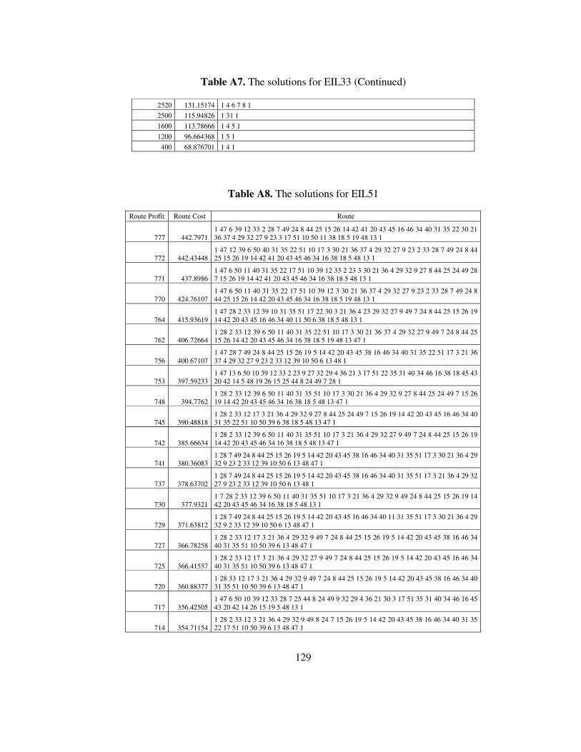
129


2520 131.15174 1 4 6 7 8 1

2500 115.94826 1 31 1

1600 113.78666 1 4 5 1

1200 96.664368 1 5 1

400 68.876701 1 4 1



777 442.7971 1 47 6 39 12 33 2 28 7 49 24 8 44 25 15 26 14 42 41 20 43 45 16 46 34 40 31 35 22 30 21 36 37 4 29 32 27 9 23 3 17 51 10 50 11 38 18 5 19 48 13 1

772 442.43448 1 47 12 39 6 50 40 31 35 22 51 10 17 3 30 21 36 37 4 29 32 27 9 23 2 33 28 7 49 24 8 44 25 15 26 19 14 42 41 20 43 45 46 34 16 38 18 5 48 13 1

771 437.8986 1 47 6 50 11 40 31 35 22 17 51 10 39 12 33 2 23 3 30 21 36 4 29 32 9 27 8 44 25 24 49 28 7 15 26 19 14 42 41 20 43 45 46 34 16 38 18 5 48 13 1

770 424.76107 1 47 6 50 11 40 31 35 22 17 51 10 39 12 3 30 21 36 37 4 29 32 27 9 23 2 33 28 7 49 24 8 44 25 15 26 14 42 20 43 45 46 34 16 38 18 5 19 48 13 1

764 415.93619 1 47 28 2 33 12 39 10 31 35 51 17 22 30 3 21 36 4 23 29 32 27 9 49 7 24 8 44 25 15 26 19 14 42 20 43 45 16 46 34 40 11 50 6 38 18 5 48 13 1

762 406.72664 1 28 2 33 12 39 6 50 11 40 31 35 22 51 10 17 3 30 21 36 37 4 29 32 27 9 49 7 24 8 44 25 15 26 14 42 20 43 45 46 34 16 38 18 5 19 48 13 47 1

756 400.67107 1 47 28 7 49 24 8 44 25 15 26 19 5 14 42 20 43 45 38 16 46 34 40 31 35 22 51 17 3 21 36 37 4 29 32 27 9 23 2 33 12 39 10 50 6 13 48 1

753 397.59233 1 47 13 6 50 10 39 12 33 2 23 9 27 32 29 4 36 21 3 17 51 22 35 31 40 34 46 16 38 18 45 43 20 42 14 5 48 19 26 15 25 44 8 24 49 7 28 1

748 394.7762 1 28 2 33 12 39 6 50 11 40 31 35 51 10 17 3 30 21 36 4 29 32 9 27 8 44 25 24 49 7 15 26 19 14 42 20 43 45 46 34 16 38 18 5 48 13 47 1

745 390.48818 1 28 2 33 12 17 3 21 36 4 29 32 9 27 8 44 25 24 49 7 15 26 19 14 42 20 43 45 16 46 34 40 31 35 22 51 10 50 39 6 38 18 5 48 13 47 1

742 385.66634 1 28 2 33 12 39 6 50 11 40 31 35 51 10 17 3 21 36 4 29 32 27 9 49 7 24 8 44 25 15 26 19 14 42 20 43 45 46 34 16 38 18 5 48 13 47 1

741 380.36083 1 28 7 49 24 8 44 25 15 26 19 5 14 42 20 43 45 38 16 46 34 40 31 35 51 17 3 30 21 36 4 29 32 9 23 2 33 12 39 10 50 6 13 48 47 1

737 378.63702 1 28 7 49 24 8 44 25 15 26 19 5 14 42 20 43 45 38 16 46 34 40 31 35 51 17 3 21 36 4 29 32 27 9 23 2 33 12 39 10 50 6 13 48 1

730 377.9321 1 7 28 2 33 12 39 6 50 11 40 31 35 51 10 17 3 21 36 4 29 32 9 49 24 8 44 25 15 26 19 14 42 20 43 45 46 34 16 38 18 5 48 13 1

729 371.63812 1 28 7 49 24 8 44 25 15 26 19 5 14 42 20 43 45 16 46 34 40 11 31 35 51 17 3 30 21 36 4 29 32 9 2 33 12 39 10 50 6 13 48 47 1

727 366.78258 1 28 2 33 12 17 3 21 36 4 29 32 9 49 7 24 8 44 25 15 26 19 5 14 42 20 43 45 38 16 46 34 40 31 35 51 10 50 39 6 13 48 47 1

725 366.41557 1 28 2 33 12 17 3 21 36 4 29 32 27 9 49 7 24 8 44 25 15 26 19 5 14 42 20 43 45 16 46 34 40 31 35 51 10 50 39 6 13 48 47 1

720 360.88377 1 28 33 12 17 3 21 36 4 29 32 9 49 7 24 8 44 25 15 26 19 5 14 42 20 43 45 38 16 46 34 40 31 35 51 10 50 39 6 13 48 47 1

717 356.42505 1 47 6 50 10 39 12 33 28 7 25 44 8 24 49 9 32 29 4 36 21 30 3 17 51 35 31 40 34 46 16 45 43 20 42 14 26 15 19 5 48 13 1

714 354.71154 1 28 2 33 12 3 21 36 4 29 32 9 49 8 24 7 15 26 19 5 14 42 20 43 45 38 16 46 34 40 31 35 22 17 51 10 50 39 6 13 48 47 1

130


710 350.36999 1 47 48 13 6 50 11 40 34 46 16 45 43 20 42 14 19 26 15 25 24 8 27 9 32 29 4 36 21 3 17 51 35 31 10 39 12 33 2 28 49 7 1

707 349.20993 1 28 33 12 39 6 50 11 40 31 35 51 10 17 3 21 36 4 29 32 9 49 8 24 7 15 26 19 14 42 20 43 45 46 34 16 38 18 5 48 13 47 1

702 337.18144 1 28 2 33 12 39 6 50 10 31 35 51 17 3 21 36 4 29 32 9 27 8 24 49 7 15 26 19 14 42 20 43 45 46 34 16 38 18 5 48 13 47 1

697 335.93656 1 28 2 33 12 39 6 50 10 31 35 51 17 3 21 36 4 29 32 9 27 8 24 49 7 15 26 19 14 42 20 43 45 46 34 16 38 18 5 48 13 1

695 331.28263 1 28 33 12 39 6 50 10 31 35 51 17 3 21 36 4 29 32 9 27 8 24 49 7 15 26 19 14 42 20 43 45 46 34 16 38 18 5 48 13 47 1

688 327.32798 1 47 28 33 12 17 3 21 36 4 29 32 9 27 8 24 49 7 15 26 19 14 42 20 43 45 16 46 34 40 31 35 51 10 50 39 6 13 48 1

686 326.61919 1 47 13 48 18 38 16 34 46 45 43 20 42 14 19 26 15 7 49 24 8 9 32 29 4 36 21 3 17 51 35 31 10 50 6 39 12 33 2 28 1

683 323.35949 1 28 33 12 39 17 3 21 36 4 29 32 9 27 8 24 49 7 15 26 19 14 42 20 43 45 16 46 34 40 31 35 51 10 50 6 13 48 1

681 316.95439 1 28 7 24 8 49 9 32 29 4 36 21 3 17 10 51 35 31 40 34 46 16 45 43 20 42 14 26 15 19 48 13 6 50 39 12 33 47 1

671 316.09264 1 28 33 12 39 6 50 10 31 35 51 17 3 21 36 4 29 32 9 49 8 24 7 15 26 19 14 42 20 43 45 46 34 16 38 13 48 1

667 314.93473 1 28 33 12 3 21 36 4 29 32 9 49 8 24 7 15 26 19 14 42 20 43 45 16 46 34 11 50 10 31 35 51 17 39 6 13 48 1

664 313.98828 1 33 12 39 6 50 10 31 35 51 17 3 21 36 4 29 32 9 49 8 24 7 15 26 19 14 42 20 43 45 46 34 16 38 18 48 13 47 1

663 313.16432 1 33 12 39 6 50 10 31 35 51 17 3 21 36 37 4 29 32 9 27 8 24 49 28 7 15 26 14 42 20 43 45 16 38 18 5 19 48 13 1

662 304.88319 1 28 2 33 12 39 6 50 10 31 35 51 17 3 21 36 4 29 32 9 49 8 24 7 15 26 14 42 20 43 45 16 38 18 5 19 48 13 47 1

655 303.56619 1 28 33 12 39 6 50 10 31 35 51 17 3 21 36 4 29 32 9 49 8 24 7 15 26 19 14 42 20 43 45 16 38 18 5 48 13 47 1

647 301.14923 1 28 33 12 39 6 50 10 31 35 51 17 3 21 36 4 29 32 9 27 8 24 49 7 15 26 19 14 42 20 43 45 38 18 5 48 13 1

645 292.97062 1 28 33 12 39 6 50 10 31 35 51 17 3 21 36 4 29 32 9 49 8 24 7 15 26 14 42 20 43 45 38 18 5 19 48 13 47 1

636 289.62139 1 28 33 12 39 6 50 10 31 35 51 17 3 21 36 4 29 32 9 8 24 49 7 15 26 14 42 20 43 45 18 5 19 48 13 47 1

629 286.88721 1 28 33 12 39 6 50 31 35 51 17 3 21 36 4 29 32 9 49 8 24 7 15 26 14 42 20 43 45 38 18 5 19 48 13 1

624 283.55297 1 28 33 12 39 6 50 10 31 35 51 17 3 21 36 4 29 32 9 27 8 24 49 7 15 26 14 42 20 43 5 19 48 13 47 1

619 282.58251 1 47 33 12 39 6 50 31 35 51 17 3 21 36 4 29 32 9 8 24 49 7 15 26 14 42 20 43 45 38 18 5 19 48 13 1

618 279.64138 1 28 2 33 12 39 6 50 10 31 35 51 17 3 21 36 4 29 32 9 27 8 24 49 7 15 26 14 42 20 5 19 48 13 47 1

610 275.96457 1 47 13 48 19 5 20 42 14 26 15 7 24 8 49 9 32 29 4 36 21 30 3 17 51 35 31 10 50 6 39 12 33 28 1

606 274.35867 1 28 33 12 39 6 50 31 35 51 17 3 21 36 4 29 32 9 8 24 49 7 15 26 14 42 20 43 5 19 48 13 47 1

602 267.43138 1 28 33 12 39 6 50 10 31 35 51 17 3 21 36 4 29 32 9 27 8 24 49 7 15 26 14 42 5 19 48 13 47 1

595 262.58971 1 28 33 12 39 6 50 10 31 35 51 17 3 21 36 4 29 32 9 49 8 24 7 15 26 14 42 5 19 48 13 47 1

578 258.30206 1 33 12 39 6 50 31 35 51 17 3 21 36 4 29 32 9 8 24 49 7 15 26 14 42 20 5 19 48 13 47 1

575 255.09862 1 33 12 39 6 50 10 31 35 51 17 3 21 36 4 29 32 9 49 8 24 7 15 26 14 42 5 19 48 13 1

569 251.7157 1 47 33 12 39 6 50 31 35 51 17 3 21 36 4 29 32 9 49 8 24 7 15 26 14 42 5 19 48 13 1

563 247.0328 1 33 12 39 6 50 10 31 35 51 17 3 21 4 29 32 9 49 8 24 7 15 26 14 42 5 19 48 13 47 1

560 245.1679 1 47 28 33 12 39 6 50 10 31 35 51 17 3 21 36 4 29 32 9 49 7 15 26 14 42 5 19 48 13 1

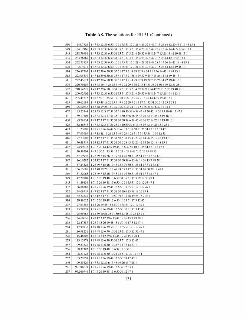
131


550 243.7326 1 47 33 12 39 6 50 10 31 35 51 17 3 21 4 29 32 9 49 7 15 26 14 42 20 43 5 19 48 13 1

549 240.7966 1 47 33 12 39 6 50 31 35 51 17 3 21 36 4 29 32 9 49 28 7 15 26 14 42 5 19 48 13 1

543 238.79986 1 47 33 12 39 6 50 31 35 51 17 3 21 4 29 32 9 49 8 24 7 15 26 14 42 19 48 13 1

535 233.26861 1 28 33 12 39 6 50 31 35 51 17 3 21 36 4 29 32 9 49 7 15 26 14 42 19 48 13 1

534 232.71929 1 47 33 12 39 6 50 10 31 35 51 17 3 21 4 29 32 9 49 28 7 15 26 14 42 19 48 13 1

528 227.611 1 47 33 12 39 6 50 10 31 35 51 17 3 21 4 29 32 9 49 7 15 26 14 42 5 19 48 13 1

514 226.87765 1 47 12 39 6 50 31 35 51 17 3 21 4 29 32 9 8 24 7 15 26 14 42 19 48 13 1

513 223.05339 1 47 12 39 6 50 31 35 51 17 3 21 36 4 29 32 9 49 7 15 26 14 42 19 48 13 1

511 222.45613 1 47 12 39 6 50 31 35 51 17 3 21 4 29 32 9 49 28 7 15 26 14 42 19 48 13 1

508 220.79259 1 13 48 19 14 26 15 7 49 9 32 29 4 36 21 3 17 51 35 31 50 6 39 12 33 28 1

507 218.54225 1 47 12 39 6 50 10 31 35 51 17 3 21 4 29 32 9 8 24 49 28 7 15 26 19 48 13 1

493 209.92902 1 47 33 12 39 6 50 31 35 51 17 3 21 4 29 32 9 49 8 24 7 15 26 19 48 13 1

471 205.41212 1 47 6 50 31 35 51 17 3 21 4 29 32 9 49 7 15 26 14 42 5 19 48 13 1

465 199.63184 1 47 13 48 19 26 15 7 49 9 32 29 4 21 3 17 51 35 31 50 6 12 33 2 28 1

459 195.60747 1 13 48 19 26 15 7 49 9 29 4 36 21 3 17 51 35 31 50 6 39 12 33 1

457 195.25544 1 28 33 12 3 17 51 35 31 10 50 39 6 38 45 43 20 42 14 26 15 19 48 13 47 1

441 189.17203 1 28 33 12 3 17 51 35 31 50 39 6 38 45 43 20 42 14 26 15 19 48 13 1

430 183.79534 1 47 12 3 17 51 35 31 10 50 39 6 38 45 43 20 42 14 26 15 19 48 13 1

425 182.46343 1 47 33 12 3 17 51 35 31 10 50 39 6 13 48 19 42 14 26 15 7 28 1

423 181.23005 1 28 7 15 26 14 42 5 19 48 13 6 39 50 31 35 51 17 3 12 33 47 1

419 177.93989 1 47 13 48 19 26 15 7 49 9 29 4 21 3 17 51 35 31 10 39 12 33 1

416 177.73007 1 33 12 3 17 51 35 31 50 6 38 45 43 20 42 14 26 15 19 48 13 47 1

411 176.48519 1 33 12 3 17 51 35 31 50 6 38 45 43 20 42 14 26 15 19 48 13 1

407 174.99032 1 7 15 26 14 42 5 19 48 13 6 39 50 10 31 35 51 17 3 12 47 1

401 170.39204 1 47 6 50 31 35 51 17 3 21 4 29 9 49 7 15 26 19 48 13 1

389 167.19946 1 28 49 7 15 26 14 19 48 13 6 50 31 35 51 17 3 12 33 47 1

387 160.6282 1 33 12 3 17 51 35 31 10 50 39 6 13 48 19 26 15 7 49 28 1

381 157.24528 1 28 49 7 15 26 19 48 13 6 39 50 31 35 51 17 3 12 33 47 1

371 156.15685 1 13 48 19 26 15 7 49 28 33 3 17 51 35 31 10 50 39 12 47 1

369 151.82065 1 28 49 7 15 26 19 48 13 6 39 50 31 35 51 17 3 12 47 1

349 147.29808 1 7 15 26 19 48 13 6 50 31 35 51 17 3 39 12 33 47 1

345 141.49834 1 7 15 26 19 48 13 6 50 10 31 35 51 17 3 12 33 47 1

337 136.88881 1 28 7 15 26 19 48 13 6 50 31 35 51 17 3 12 47 1

322 134.08919 1 47 12 3 17 51 35 31 50 39 6 13 48 19 26 15 1

318 132.22821 1 47 12 3 17 51 10 50 39 6 13 48 19 26 15 7 28 1

314 129.88022 1 7 15 26 19 48 13 6 50 10 35 51 17 3 12 47 1

307 127.64856 1 15 26 19 48 13 6 50 31 35 51 17 3 12 47 1

303 125.78758 1 28 7 15 26 19 48 13 6 50 10 51 17 3 12 47 1

298 125.65683 1 12 39 10 51 35 31 50 6 13 48 19 26 15 7 1

296 124.60636 1 47 12 3 17 39 6 13 48 19 26 15 7 49 28 1

293 122.47387 1 28 7 15 26 19 48 13 6 50 10 17 3 12 47 1

284 117.99831 1 19 48 13 6 39 50 10 31 35 51 17 3 12 47 1

281 116.98231 1 19 48 13 6 50 10 31 35 51 17 3 12 33 47 1

276 115.48307 1 47 33 3 12 39 6 13 48 19 26 15 7 28 1

273 113.15978 1 19 48 13 6 39 50 31 35 51 17 3 12 47 1

257 109.33321 1 19 48 13 6 50 10 35 51 17 3 12 33 1

256 108.37382 1 7 15 26 19 48 13 6 39 12 3 33 1

254 108.31128 1 19 48 13 6 50 10 31 35 51 17 39 12 47 1

252 103.22058 1 28 7 15 26 19 48 13 6 50 39 12 47 1

246 99.85429 1 47 33 12 39 6 13 48 19 26 15 7 28 1

241 98.398678 1 28 7 15 26 19 48 13 6 39 12 33 1

237 97.566946 1 7 15 26 19 48 13 6 50 39 12 47 1

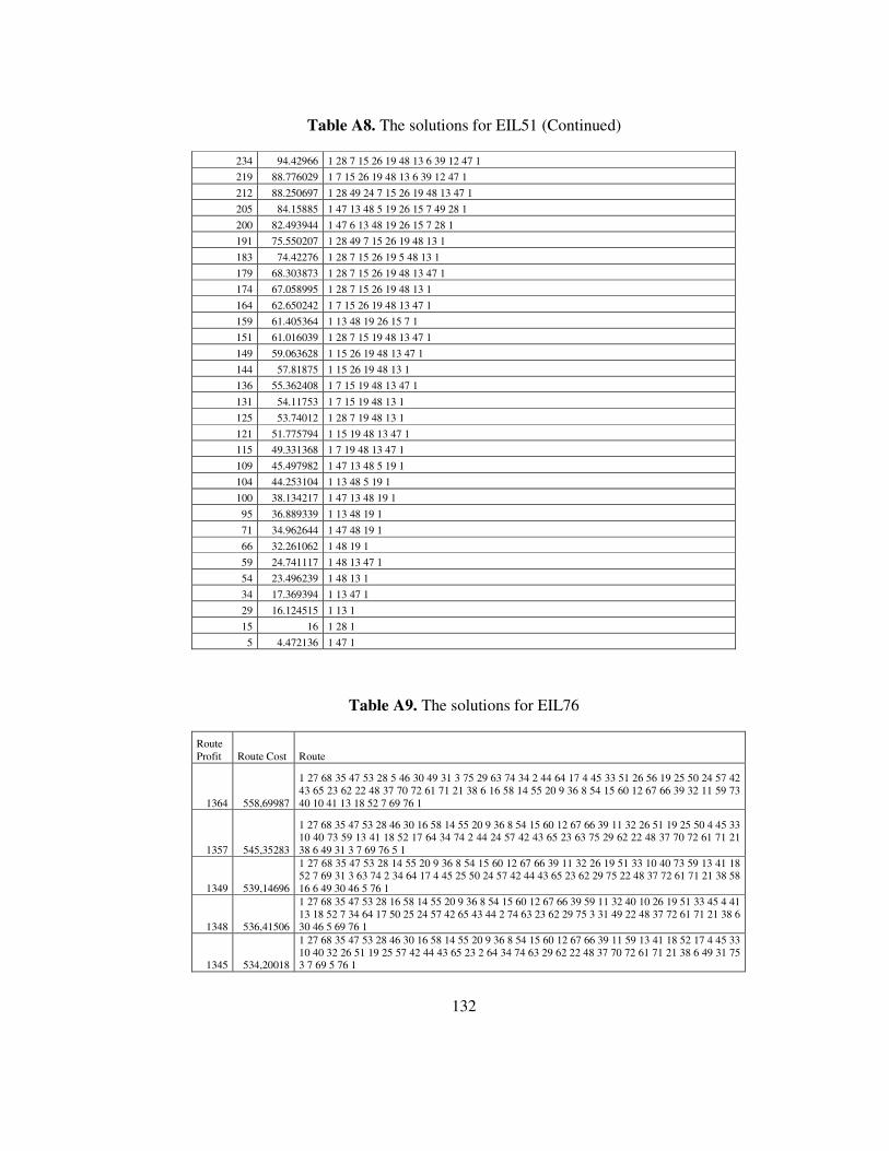
132


234 94.42966 1 28 7 15 26 19 48 13 6 39 12 47 1

219 88.776029 1 7 15 26 19 48 13 6 39 12 47 1

212 88.250697 1 28 49 24 7 15 26 19 48 13 47 1

205 84.15885 1 47 13 48 5 19 26 15 7 49 28 1

200 82.493944 1 47 6 13 48 19 26 15 7 28 1

191 75.550207 1 28 49 7 15 26 19 48 13 1

183 74.42276 1 28 7 15 26 19 5 48 13 1

179 68.303873 1 28 7 15 26 19 48 13 47 1

174 67.058995 1 28 7 15 26 19 48 13 1

164 62.650242 1 7 15 26 19 48 13 47 1

159 61.405364 1 13 48 19 26 15 7 1

151 61.016039 1 28 7 15 19 48 13 47 1

149 59.063628 1 15 26 19 48 13 47 1

144 57.81875 1 15 26 19 48 13 1

136 55.362408 1 7 15 19 48 13 47 1

131 54.11753 1 7 15 19 48 13 1

125 53.74012 1 28 7 19 48 13 1

121 51.775794 1 15 19 48 13 47 1

115 49.331368 1 7 19 48 13 47 1

109 45.497982 1 47 13 48 5 19 1

104 44.253104 1 13 48 5 19 1

100 38.134217 1 47 13 48 19 1

95 36.889339 1 13 48 19 1

71 34.962644 1 47 48 19 1

66 32.261062 1 48 19 1

59 24.741117 1 48 13 47 1

54 23.496239 1 48 13 1

34 17.369394 1 13 47 1

29 16.124515 1 13 1

15 16 1 28 1

5 4.472136 1 47 1



1364 558,69987

1 27 68 35 47 53 28 5 46 30 49 31 3 75 29 63 74 34 2 44 64 17 4 45 33 51 26 56 19 25 50 24 57 42 43 65 23 62 22 48 37 70 72 61 71 21 38 6 16 58 14 55 20 9 36 8 54 15 60 12 67 66 39 32 11 59 73 40 10 41 13 18 52 7 69 76 1

1357 545,35283

1 27 68 35 47 53 28 46 30 16 58 14 55 20 9 36 8 54 15 60 12 67 66 39 11 32 26 51 19 25 50 4 45 33 10 40 73 59 13 41 18 52 17 64 34 74 2 44 24 57 42 43 65 23 63 75 29 62 22 48 37 70 72 61 71 21 38 6 49 31 3 7 69 76 5 1

1349 539,14696

1 27 68 35 47 53 28 14 55 20 9 36 8 54 15 60 12 67 66 39 11 32 26 19 51 33 10 40 73 59 13 41 18 52 7 69 31 3 63 74 2 34 64 17 4 45 25 50 24 57 42 44 43 65 23 62 29 75 22 48 37 72 61 71 21 38 58 16 6 49 30 46 5 76 1

1348 536,41506

1 27 68 35 47 53 28 16 58 14 55 20 9 36 8 54 15 60 12 67 66 39 59 11 32 40 10 26 19 51 33 45 4 41 13 18 52 7 34 64 17 50 25 24 57 42 65 43 44 2 74 63 23 62 29 75 3 31 49 22 48 37 72 61 71 21 38 6 30 46 5 69 76 1

1345 534,20018

1 27 68 35 47 53 28 46 30 16 58 14 55 20 9 36 8 54 15 60 12 67 66 39 11 59 13 41 18 52 17 4 45 33 10 40 32 26 51 19 25 57 42 44 43 65 23 2 64 34 74 63 29 62 22 48 37 70 72 61 71 21 38 6 49 31 75 3 7 69 5 76 1

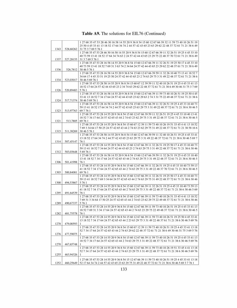
133


1343 528,68262

1 27 68 35 47 53 28 46 30 16 58 14 55 20 9 36 8 54 15 60 12 67 66 39 32 11 59 73 40 10 26 51 19 25 50 4 45 33 41 13 18 52 17 64 34 74 2 44 57 42 43 65 23 63 29 62 22 48 37 72 61 71 21 38 6 49 31 75 3 7 69 5 76 1

1337 527,28155

1 27 68 35 47 53 28 46 30 16 58 14 55 20 9 36 8 54 15 60 12 67 66 39 11 32 26 51 19 25 4 45 33 10 40 73 59 13 41 18 52 17 64 34 74 63 2 24 57 42 44 43 65 23 29 75 22 48 37 70 72 61 71 21 38 6 49 31 3 7 69 5 76 1

1336 526,7812

1 27 68 35 47 53 28 16 58 14 55 20 9 36 8 54 15 60 12 67 66 39 11 32 26 51 19 25 50 17 4 45 33 10 40 73 59 13 41 18 52 7 69 31 3 63 74 2 34 64 24 57 42 44 43 65 23 29 62 22 48 37 61 71 21 38 6 49 30 46 5 76 1

1334 523,03017

1 27 68 35 47 53 28 16 58 14 55 20 9 36 8 54 15 60 12 67 66 39 59 11 32 26 10 40 73 13 41 18 52 7 34 64 17 4 45 33 51 19 25 50 24 57 42 44 43 65 23 2 74 63 29 75 3 31 49 22 48 37 72 61 71 21 38 6 30 46 5 69 76 1

1326 520,89483

1 27 68 35 47 53 28 58 14 55 20 9 36 8 54 15 60 67 12 39 59 11 32 40 10 26 51 19 25 4 45 33 41 13 18 52 17 64 24 57 42 44 43 65 23 2 34 74 63 29 62 22 48 37 72 61 71 21 38 6 49 30 46 31 75 3 7 69 5 76 1

1324 517,71374

1 27 68 35 47 53 28 16 58 14 55 20 9 36 8 54 15 60 12 67 66 39 11 59 73 40 10 26 51 19 25 50 4 45 33 41 13 18 52 7 34 17 64 24 57 42 44 43 65 23 62 29 63 2 74 3 31 75 22 49 48 37 72 61 71 21 38 6 30 46 5 69 76 1

1323 513,97763

1 27 68 35 47 53 28 16 58 14 55 20 9 36 8 54 15 60 12 67 66 39 11 32 26 51 19 25 4 45 33 10 40 73 59 13 41 18 52 17 64 34 74 2 44 57 42 43 65 23 63 29 75 3 31 49 22 48 37 72 61 71 21 38 6 30 46 5 69 7 76 1

1321 513,7805

1 27 68 35 47 53 28 14 55 20 9 36 8 54 15 60 12 67 66 39 59 11 32 26 51 19 25 4 45 33 10 40 13 41 18 52 7 34 17 64 24 57 42 65 43 44 2 74 63 23 62 29 75 3 31 49 22 48 37 72 61 71 21 38 6 30 46 5 69 76 1

1315 511,38269

1 27 68 35 47 53 28 14 55 20 9 36 8 54 15 60 67 12 39 11 59 73 40 10 26 19 51 33 45 4 41 13 18 52 7 69 3 34 64 17 50 25 24 57 42 65 43 44 2 74 63 23 62 29 75 31 49 22 48 37 72 61 71 21 38 58 16 6 30 46 5 76 1

1314 507,45147

1 27 68 35 47 53 28 58 14 55 20 9 36 8 54 15 60 12 67 66 39 59 11 32 40 10 26 51 19 25 4 45 33 41 13 18 52 17 64 34 74 2 44 57 42 43 65 23 63 29 75 3 31 49 22 48 37 72 61 71 21 38 6 30 46 5 69 7 76 1

1312 503,03648

1 27 68 35 47 53 28 14 55 20 9 36 8 54 15 60 12 67 66 39 11 32 26 51 19 25 50 17 4 45 33 10 40 73 59 13 41 18 52 7 34 64 24 57 42 44 43 65 23 2 74 63 29 75 3 31 49 22 48 37 72 61 71 21 38 6 30 46 5 69 76 1

1306 501,41998

1 27 68 35 47 53 28 16 58 14 55 20 9 36 8 54 15 60 12 67 66 39 59 11 32 26 51 19 25 4 45 33 10 40 13 41 18 52 7 34 17 64 24 57 42 65 43 44 2 74 63 29 75 3 31 49 22 48 37 72 61 71 21 38 6 30 46 5 76 1

1303 500,84081

1 27 68 35 47 53 28 14 55 20 9 36 8 54 15 60 12 67 66 39 11 32 26 51 19 25 4 45 33 10 40 73 59 13 41 18 52 7 34 17 64 24 57 42 65 43 44 2 74 63 29 75 3 31 49 22 48 37 70 72 61 71 21 38 6 30 46 5 69 76 1

1300 494,53867

1 27 68 35 47 53 28 14 55 20 9 36 8 54 15 60 12 67 66 39 11 32 26 51 19 25 50 17 4 45 33 10 40 73 59 13 41 18 52 7 69 3 34 64 24 57 42 65 43 44 2 74 63 29 75 31 49 22 48 37 72 61 71 21 38 6 30 46 5 76 1

1295 491,64539

1 27 68 35 47 53 28 14 55 20 9 36 8 54 15 60 12 67 66 39 11 32 26 51 19 25 4 45 33 10 40 73 59 13 41 18 52 7 34 17 64 24 57 42 65 43 44 2 74 63 29 75 3 31 49 22 48 37 72 61 71 21 38 6 30 46 5 69 76 1

1289 490,67337

1 27 68 35 47 53 28 14 55 20 9 36 8 54 15 60 12 67 66 39 11 59 73 40 10 26 51 33 45 4 41 13 18 52 7 69 31 3 34 64 17 50 25 24 57 42 65 43 44 2 74 63 23 62 29 75 22 49 48 37 72 61 71 21 38 6 30 46 5 76 1

1282 481,75578

1 27 68 35 47 53 28 14 55 20 9 36 8 54 15 60 12 67 66 39 11 59 73 40 10 26 51 19 25 4 45 33 41 13 18 52 7 69 31 3 34 17 64 24 57 42 65 43 44 2 74 63 23 29 75 22 49 48 37 72 61 71 21 38 6 30 46 5 76 1

1278 479,00593

1 27 68 35 47 53 28 14 55 20 9 36 8 54 15 60 12 67 66 39 11 59 73 40 10 26 51 19 25 50 4 45 33 41 13 18 52 7 34 17 64 24 57 42 65 43 44 2 23 63 29 75 3 31 49 22 48 37 61 71 21 38 6 30 46 5 69 76 1

1276 477,59075

1 27 68 35 47 53 28 14 55 20 9 36 8 54 15 60 67 12 39 11 59 73 40 10 26 51 19 25 4 45 33 41 13 18 52 7 34 17 64 24 57 42 65 43 44 2 74 63 29 62 22 48 37 72 61 71 21 38 6 49 30 46 31 75 3 69 5 76 1

1270 467,65748

1 27 68 35 47 53 28 14 55 20 9 36 8 54 15 60 12 67 66 39 11 59 73 40 10 26 51 19 25 4 45 33 41 13 18 52 7 34 17 64 24 57 42 65 43 44 2 74 63 29 75 3 31 49 22 48 37 72 61 71 21 38 6 30 46 5 69 76 1

1255 463,94326

1 27 68 35 47 53 28 14 55 20 9 36 8 54 15 60 12 67 66 39 11 59 73 40 10 26 19 51 33 45 4 41 13 18 52 7 34 17 64 24 57 42 65 43 44 2 74 63 23 29 75 3 31 49 22 48 37 72 61 71 21 38 6 30 46 5 69 76 1

1252 460,25649 1 27 68 35 47 53 28 14 55 20 9 36 8 54 15 12 67 66 39 11 59 73 40 10 26 51 19 25 4 45 33 41 13 18 52 17 64 34 74 2 44 57 42 43 65 23 63 29 75 31 49 22 48 37 72 61 71 21 38 6 30 46 5 69 3 7 76 1

134


1236 458,38833 1 68 27 18 13 41 10 40 32 11 59 39 66 67 12 60 15 54 8 36 9 47 35 53 28 46 30 49 6 38 21 71 61 72 37 48 22 62 29 63 74 34 64 2 44 43 65 42 57 25 19 51 33 45 4 17 52 7 69 3 31 5 76 1

1230 443,7298 1 27 68 35 47 53 28 14 55 20 9 36 8 54 15 60 12 67 66 39 11 59 73 40 10 26 51 33 45 4 41 13 18 52 7 34 17 64 24 57 42 65 43 44 2 74 63 29 75 3 31 49 22 48 37 72 61 71 21 38 6 30 46 5 69 76 1

1212 433,90337 1 68 27 8 36 9 47 35 53 28 14 55 20 15 54 12 67 66 39 11 59 73 40 10 26 51 33 45 4 41 13 18 52 7 34 64 17 50 25 57 42 65 43 44 2 74 63 29 3 31 49 22 48 37 72 61 71 21 38 6 30 46 5 76 1

1208 430,32314 1 68 27 8 36 9 47 35 53 28 14 55 20 15 54 12 67 66 39 11 59 73 40 10 26 51 19 25 4 45 33 41 13 18 52 7 34 17 64 24 57 42 43 44 2 74 63 29 3 31 49 22 48 37 72 61 71 21 38 6 30 46 5 69 76 1

1192 424,97807 1 27 68 35 47 9 20 36 8 54 15 60 12 67 66 39 11 59 73 40 10 26 51 33 45 4 41 13 18 52 7 34 17 64 24 57 42 65 43 44 2 74 63 29 75 3 31 49 22 48 37 72 61 71 21 38 6 30 46 28 53 5 76 1

1186 424,62843 1 27 68 35 47 9 8 36 20 15 54 12 67 66 39 11 59 73 40 10 51 33 45 4 41 13 18 52 7 34 17 64 24 57 42 65 43 44 2 74 63 29 75 3 31 49 22 48 37 72 61 71 21 38 58 16 6 30 46 28 53 5 69 76 1

1185 424,56567 1 27 68 47 8 36 9 20 15 54 12 67 66 39 11 59 73 40 10 51 33 45 4 41 13 18 52 17 50 25 24 57 42 65 43 44 2 34 74 63 29 75 22 48 37 72 61 71 21 38 6 49 30 46 28 53 35 5 31 3 7 69 76 1

1184 420,90985 1 27 68 35 47 9 8 36 20 15 54 12 67 66 39 11 59 73 40 10 26 51 33 45 4 41 13 18 52 7 34 17 64 2 44 24 57 42 43 65 23 63 29 75 3 31 49 22 48 37 72 61 71 21 38 6 30 46 28 53 5 69 76 1

1178 419,45023 1 27 68 35 47 53 28 14 55 20 9 36 8 54 15 60 67 12 39 11 59 73 40 10 51 33 45 4 41 13 18 52 7 34 64 24 57 42 65 43 44 2 74 63 3 31 75 29 22 48 37 72 61 71 21 38 6 49 30 46 5 76 1

1175 416,88285 1 27 68 35 47 53 28 14 55 20 9 36 8 54 15 60 67 12 39 11 59 73 40 10 26 19 51 33 45 4 41 13 18 52 7 34 17 64 24 57 42 44 2 74 63 29 3 31 49 22 48 37 72 61 71 21 38 6 30 46 5 76 1

1173 414,30918 1 27 68 35 47 9 36 8 54 15 60 12 67 66 39 11 59 73 40 10 51 33 45 4 41 13 18 52 7 34 17 64 24 57 42 65 43 44 2 74 63 29 75 3 31 49 22 48 37 72 61 71 21 38 6 30 46 28 53 5 69 76 1

1168 408,84486 1 27 68 47 35 28 53 9 8 36 20 15 54 12 67 66 39 11 59 73 40 10 26 51 33 45 4 41 13 18 52 7 34 17 64 24 57 42 65 43 44 2 74 63 29 75 3 31 49 22 48 37 72 61 71 21 38 6 30 46 5 76 1

1161 408,02379 1 27 68 35 47 53 28 14 55 20 9 36 8 54 15 12 67 66 39 11 59 73 40 10 26 51 33 45 4 41 13 18 52 7 34 64 24 57 42 65 43 44 2 63 29 3 31 49 22 48 37 72 61 71 21 38 6 30 46 5 76 1

1160 406,97744 1 27 68 35 47 9 36 8 54 15 12 67 66 39 11 59 73 40 10 26 19 51 33 45 4 41 13 18 52 7 34 17 64 24 57 42 65 43 44 2 63 29 75 3 31 49 22 48 37 72 61 71 21 38 6 30 46 28 53 5 76 1

1154 403,95529 1 27 68 35 47 9 36 8 54 15 60 67 12 39 11 59 73 40 10 51 33 45 4 41 13 18 52 7 34 17 64 24 57 42 65 43 44 2 74 63 29 75 3 31 49 22 48 37 72 61 71 21 38 6 30 46 28 53 5 76 1

1142 396,26543 1 27 68 47 35 28 53 9 8 36 20 15 54 12 67 66 39 11 59 73 40 10 33 45 4 41 13 18 52 7 34 17 64 24 57 42 65 43 44 2 74 63 29 75 3 31 49 22 48 37 72 61 71 21 38 6 30 46 5 69 76 1

1130 388,43885 1 27 68 35 47 8 9 20 15 54 12 67 66 39 11 59 73 40 10 26 51 33 45 4 41 13 18 52 7 34 17 64 24 57 42 43 44 2 74 63 29 75 3 31 49 22 48 37 72 61 71 21 38 6 30 46 28 53 5 76 1

1119 382,46053 1 27 68 47 35 28 53 9 36 8 54 15 12 67 66 39 11 59 73 40 10 26 51 33 45 4 41 13 18 52 7 34 17 64 24 57 42 43 44 2 63 29 75 3 31 49 22 48 37 72 61 71 21 38 6 30 46 5 76 1

1115 378,30552 1 27 68 35 47 9 20 15 54 12 67 66 39 11 59 73 40 10 26 51 33 45 4 41 13 18 52 7 34 17 64 24 57 42 43 44 2 74 63 29 75 3 31 49 22 48 37 72 61 71 21 38 6 30 46 28 53 5 76 1

1101 372,8532 1 27 68 35 47 9 8 54 15 12 67 66 39 11 59 73 40 10 51 33 45 4 41 13 18 52 7 34 17 64 24 57 42 43 44 2 74 63 29 75 3 31 49 22 48 37 72 61 71 21 38 6 30 46 28 53 5 76 1

1099 372,47875 1 27 68 35 47 9 36 8 54 15 12 67 66 39 11 59 73 40 10 33 45 4 41 13 18 52 17 64 24 57 42 43 44 2 34 74 63 29 75 3 31 49 22 48 37 72 61 71 21 38 6 30 46 28 53 5 76 69 7 1

1089 362,17265 1 68 35 47 9 20 15 54 12 67 66 39 11 59 73 40 10 33 45 4 17 64 24 57 42 43 44 2 34 74 63 29 75 3 31 49 22 48 37 72 61 71 21 38 6 30 46 28 53 5 76 69 7 52 18 41 13 27 1

1073 361,35463 1 27 68 47 9 36 8 54 15 12 67 66 39 11 59 73 40 10 51 33 45 4 41 13 18 52 7 34 17 64 24 57 42 44 2 74 63 29 75 3 31 49 22 48 37 21 38 6 30 46 28 53 35 5 76 1

1065 356,60698 1 27 68 35 47 9 36 8 54 15 12 67 66 39 11 59 73 40 10 51 33 45 4 41 13 18 52 7 34 64 24 57 42 44 2 63 29 3 31 49 22 48 37 72 61 71 21 38 6 30 46 28 53 5 76 1

1048 353,03282 1 27 68 47 35 28 53 9 36 54 15 60 12 67 66 39 11 59 73 40 10 26 51 33 45 4 41 13 18 52 7 34 17 64 24 57 42 44 2 74 63 29 75 3 31 49 22 48 6 30 46 5 76 1

1044 351,19867 1 68 27 8 47 35 28 53 9 20 15 54 12 67 66 39 11 59 73 40 10 26 51 33 45 4 41 13 18 52 7 34 17 64 24 57 42 44 2 74 63 29 75 3 31 49 22 48 6 30 46 5 76 1

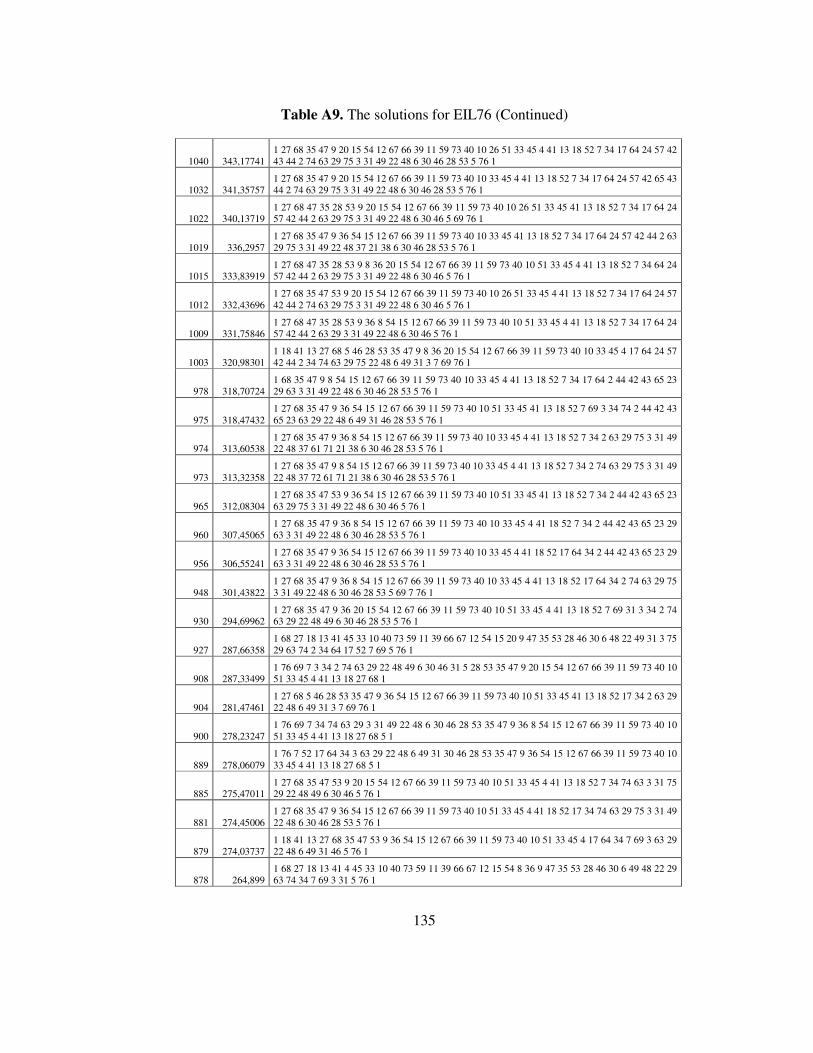
135


1040 343,17741 1 27 68 35 47 9 20 15 54 12 67 66 39 11 59 73 40 10 26 51 33 45 4 41 13 18 52 7 34 17 64 24 57 42 43 44 2 74 63 29 75 3 31 49 22 48 6 30 46 28 53 5 76 1

1032 341,35757 1 27 68 35 47 9 20 15 54 12 67 66 39 11 59 73 40 10 33 45 4 41 13 18 52 7 34 17 64 24 57 42 65 43 44 2 74 63 29 75 3 31 49 22 48 6 30 46 28 53 5 76 1

1022 340,13719 1 27 68 47 35 28 53 9 20 15 54 12 67 66 39 11 59 73 40 10 26 51 33 45 41 13 18 52 7 34 17 64 24 57 42 44 2 63 29 75 3 31 49 22 48 6 30 46 5 69 76 1

1019 336,2957 1 27 68 35 47 9 36 54 15 12 67 66 39 11 59 73 40 10 33 45 41 13 18 52 7 34 17 64 24 57 42 44 2 63 29 75 3 31 49 22 48 37 21 38 6 30 46 28 53 5 76 1

1015 333,83919 1 27 68 47 35 28 53 9 8 36 20 15 54 12 67 66 39 11 59 73 40 10 51 33 45 4 41 13 18 52 7 34 64 24 57 42 44 2 63 29 75 3 31 49 22 48 6 30 46 5 76 1

1012 332,43696 1 27 68 35 47 53 9 20 15 54 12 67 66 39 11 59 73 40 10 26 51 33 45 4 41 13 18 52 7 34 17 64 24 57 42 44 2 74 63 29 75 3 31 49 22 48 6 30 46 5 76 1

1009 331,75846 1 27 68 47 35 28 53 9 36 8 54 15 12 67 66 39 11 59 73 40 10 51 33 45 4 41 13 18 52 7 34 17 64 24 57 42 44 2 63 29 3 31 49 22 48 6 30 46 5 76 1

1003 320,98301 1 18 41 13 27 68 5 46 28 53 35 47 9 8 36 20 15 54 12 67 66 39 11 59 73 40 10 33 45 4 17 64 24 57 42 44 2 34 74 63 29 75 22 48 6 49 31 3 7 69 76 1

978 318,70724 1 68 35 47 9 8 54 15 12 67 66 39 11 59 73 40 10 33 45 4 41 13 18 52 7 34 17 64 2 44 42 43 65 23 29 63 3 31 49 22 48 6 30 46 28 53 5 76 1

975 318,47432 1 27 68 35 47 9 36 54 15 12 67 66 39 11 59 73 40 10 51 33 45 41 13 18 52 7 69 3 34 74 2 44 42 43 65 23 63 29 22 48 6 49 31 46 28 53 5 76 1

974 313,60538 1 27 68 35 47 9 36 8 54 15 12 67 66 39 11 59 73 40 10 33 45 4 41 13 18 52 7 34 2 63 29 75 3 31 49 22 48 37 61 71 21 38 6 30 46 28 53 5 76 1

973 313,32358 1 27 68 35 47 9 8 54 15 12 67 66 39 11 59 73 40 10 33 45 4 41 13 18 52 7 34 2 74 63 29 75 3 31 49 22 48 37 72 61 71 21 38 6 30 46 28 53 5 76 1

965 312,08304 1 27 68 35 47 53 9 36 54 15 12 67 66 39 11 59 73 40 10 51 33 45 41 13 18 52 7 34 2 44 42 43 65 23 63 29 75 3 31 49 22 48 6 30 46 5 76 1

960 307,45065 1 27 68 35 47 9 36 8 54 15 12 67 66 39 11 59 73 40 10 33 45 4 41 18 52 7 34 2 44 42 43 65 23 29 63 3 31 49 22 48 6 30 46 28 53 5 76 1

956 306,55241 1 27 68 35 47 9 36 54 15 12 67 66 39 11 59 73 40 10 33 45 4 41 18 52 17 64 34 2 44 42 43 65 23 29 63 3 31 49 22 48 6 30 46 28 53 5 76 1

948 301,43822 1 27 68 35 47 9 36 8 54 15 12 67 66 39 11 59 73 40 10 33 45 4 41 13 18 52 17 64 34 2 74 63 29 75 3 31 49 22 48 6 30 46 28 53 5 69 7 76 1

930 294,69962 1 27 68 35 47 9 36 20 15 54 12 67 66 39 11 59 73 40 10 51 33 45 4 41 13 18 52 7 69 31 3 34 2 74 63 29 22 48 49 6 30 46 28 53 5 76 1

927 287,66358 1 68 27 18 13 41 45 33 10 40 73 59 11 39 66 67 12 54 15 20 9 47 35 53 28 46 30 6 48 22 49 31 3 75 29 63 74 2 34 64 17 52 7 69 5 76 1

908 287,33499 1 76 69 7 3 34 2 74 63 29 22 48 49 6 30 46 31 5 28 53 35 47 9 20 15 54 12 67 66 39 11 59 73 40 10 51 33 45 4 41 13 18 27 68 1

904 281,47461 1 27 68 5 46 28 53 35 47 9 36 54 15 12 67 66 39 11 59 73 40 10 51 33 45 41 13 18 52 17 34 2 63 29 22 48 6 49 31 3 7 69 76 1

900 278,23247 1 76 69 7 34 74 63 29 3 31 49 22 48 6 30 46 28 53 35 47 9 36 8 54 15 12 67 66 39 11 59 73 40 10 51 33 45 4 41 13 18 27 68 5 1

889 278,06079 1 76 7 52 17 64 34 3 63 29 22 48 6 49 31 30 46 28 53 35 47 9 36 54 15 12 67 66 39 11 59 73 40 10 33 45 4 41 13 18 27 68 5 1

885 275,47011 1 27 68 35 47 53 9 20 15 54 12 67 66 39 11 59 73 40 10 51 33 45 4 41 13 18 52 7 34 74 63 3 31 75 29 22 48 49 6 30 46 5 76 1

881 274,45006 1 27 68 35 47 9 36 54 15 12 67 66 39 11 59 73 40 10 51 33 45 4 41 18 52 17 34 74 63 29 75 3 31 49 22 48 6 30 46 28 53 5 76 1

879 274,03737 1 18 41 13 27 68 35 47 53 9 36 54 15 12 67 66 39 11 59 73 40 10 51 33 45 4 17 64 34 7 69 3 63 29 22 48 6 49 31 46 5 76 1

878 264,899 1 68 27 18 13 41 4 45 33 10 40 73 59 11 39 66 67 12 15 54 8 36 9 47 35 53 28 46 30 6 49 48 22 29 63 74 34 7 69 3 31 5 76 1

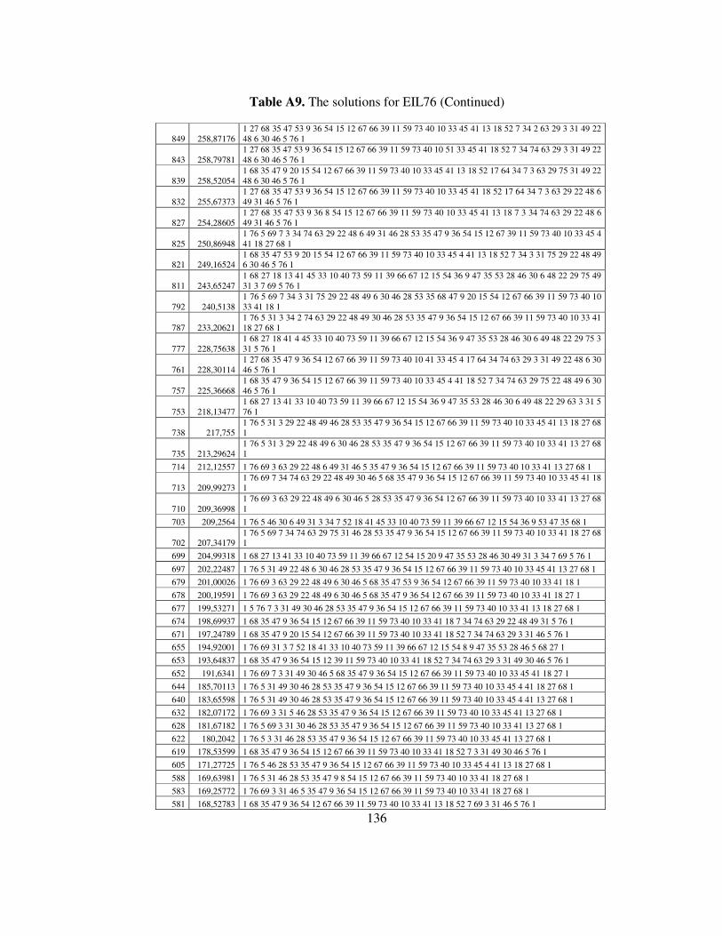
136


849 258,87176 1 27 68 35 47 53 9 36 54 15 12 67 66 39 11 59 73 40 10 33 45 41 13 18 52 7 34 2 63 29 3 31 49 22 48 6 30 46 5 76 1

843 258,79781 1 27 68 35 47 53 9 36 54 15 12 67 66 39 11 59 73 40 10 51 33 45 41 18 52 7 34 74 63 29 3 31 49 22 48 6 30 46 5 76 1

839 258,52054 1 68 35 47 9 20 15 54 12 67 66 39 11 59 73 40 10 33 45 41 13 18 52 17 64 34 7 3 63 29 75 31 49 22 48 6 30 46 5 76 1

832 255,67373 1 27 68 35 47 53 9 36 54 15 12 67 66 39 11 59 73 40 10 33 45 41 18 52 17 64 34 7 3 63 29 22 48 6 49 31 46 5 76 1

827 254,28605 1 27 68 35 47 53 9 36 8 54 15 12 67 66 39 11 59 73 40 10 33 45 41 13 18 7 3 34 74 63 29 22 48 6 49 31 46 5 76 1

825 250,86948 1 76 5 69 7 3 34 74 63 29 22 48 6 49 31 46 28 53 35 47 9 36 54 15 12 67 39 11 59 73 40 10 33 45 4 41 18 27 68 1

821 249,16524 1 68 35 47 53 9 20 15 54 12 67 66 39 11 59 73 40 10 33 45 4 41 13 18 52 7 34 3 31 75 29 22 48 49 6 30 46 5 76 1

811 243,65247 1 68 27 18 13 41 45 33 10 40 73 59 11 39 66 67 12 15 54 36 9 47 35 53 28 46 30 6 48 22 29 75 49 31 3 7 69 5 76 1

792 240,5138 1 76 5 69 7 34 3 31 75 29 22 48 49 6 30 46 28 53 35 68 47 9 20 15 54 12 67 66 39 11 59 73 40 10 33 41 18 1

787 233,20621 1 76 5 31 3 34 2 74 63 29 22 48 49 30 46 28 53 35 47 9 36 54 15 12 67 66 39 11 59 73 40 10 33 41 18 27 68 1

777 228,75638 1 68 27 18 41 4 45 33 10 40 73 59 11 39 66 67 12 15 54 36 9 47 35 53 28 46 30 6 49 48 22 29 75 3 31 5 76 1

761 228,30114 1 27 68 35 47 9 36 54 12 67 66 39 11 59 73 40 10 41 33 45 4 17 64 34 74 63 29 3 31 49 22 48 6 30 46 5 76 1

757 225,36668 1 68 35 47 9 36 54 15 12 67 66 39 11 59 73 40 10 33 45 4 41 18 52 7 34 74 63 29 75 22 48 49 6 30 46 5 76 1

753 218,13477 1 68 27 13 41 33 10 40 73 59 11 39 66 67 12 15 54 36 9 47 35 53 28 46 30 6 49 48 22 29 63 3 31 5 76 1

738 217,755 1 76 5 31 3 29 22 48 49 46 28 53 35 47 9 36 54 15 12 67 66 39 11 59 73 40 10 33 45 41 13 18 27 68 1

735 213,29624 1 76 5 31 3 29 22 48 49 6 30 46 28 53 35 47 9 36 54 15 12 67 66 39 11 59 73 40 10 33 41 13 27 68 1

714 212,12557 1 76 69 3 63 29 22 48 6 49 31 46 5 35 47 9 36 54 15 12 67 66 39 11 59 73 40 10 33 41 13 27 68 1

713 209,99273 1 76 69 7 34 74 63 29 22 48 49 30 46 5 68 35 47 9 36 54 15 12 67 66 39 11 59 73 40 10 33 45 41 18 1

710 209,36998 1 76 69 3 63 29 22 48 49 6 30 46 5 28 53 35 47 9 36 54 12 67 66 39 11 59 73 40 10 33 41 13 27 68 1

703 209,2564 1 76 5 46 30 6 49 31 3 34 7 52 18 41 45 33 10 40 73 59 11 39 66 67 12 15 54 36 9 53 47 35 68 1

702 207,34179 1 76 5 69 7 34 74 63 29 75 31 46 28 53 35 47 9 36 54 15 12 67 66 39 11 59 73 40 10 33 41 18 27 68 1

699 204,99318 1 68 27 13 41 33 10 40 73 59 11 39 66 67 12 54 15 20 9 47 35 53 28 46 30 49 31 3 34 7 69 5 76 1

697 202,22487 1 76 5 31 49 22 48 6 30 46 28 53 35 47 9 36 54 15 12 67 66 39 11 59 73 40 10 33 45 41 13 27 68 1

679 201,00026 1 76 69 3 63 29 22 48 49 6 30 46 5 68 35 47 53 9 36 54 12 67 66 39 11 59 73 40 10 33 41 18 1

678 200,19591 1 76 69 3 63 29 22 48 49 6 30 46 5 68 35 47 9 36 54 12 67 66 39 11 59 73 40 10 33 41 18 27 1

677 199,53271 1 5 76 7 3 31 49 30 46 28 53 35 47 9 36 54 15 12 67 66 39 11 59 73 40 10 33 41 13 18 27 68 1

674 198,69937 1 68 35 47 9 36 54 15 12 67 66 39 11 59 73 40 10 33 41 18 7 34 74 63 29 22 48 49 31 5 76 1

671 197,24789 1 68 35 47 9 20 15 54 12 67 66 39 11 59 73 40 10 33 41 18 52 7 34 74 63 29 3 31 46 5 76 1

655 194,92001 1 76 69 31 3 7 52 18 41 33 10 40 73 59 11 39 66 67 12 15 54 8 9 47 35 53 28 46 5 68 27 1

653 193,64837 1 68 35 47 9 36 54 15 12 39 11 59 73 40 10 33 41 18 52 7 34 74 63 29 3 31 49 30 46 5 76 1

652 191,6341 1 76 69 7 3 31 49 30 46 5 68 35 47 9 36 54 15 12 67 66 39 11 59 73 40 10 33 45 41 18 27 1

644 185,70113 1 76 5 31 49 30 46 28 53 35 47 9 36 54 15 12 67 66 39 11 59 73 40 10 33 45 4 41 18 27 68 1

640 183,65598 1 76 5 31 49 30 46 28 53 35 47 9 36 54 15 12 67 66 39 11 59 73 40 10 33 45 4 41 13 27 68 1

632 182,07172 1 76 69 3 31 5 46 28 53 35 47 9 36 54 15 12 67 66 39 11 59 73 40 10 33 45 41 13 27 68 1

628 181,67182 1 76 5 69 3 31 30 46 28 53 35 47 9 36 54 15 12 67 66 39 11 59 73 40 10 33 41 13 27 68 1

622 180,2042 1 76 5 3 31 46 28 53 35 47 9 36 54 15 12 67 66 39 11 59 73 40 10 33 45 41 13 27 68 1

619 178,53599 1 68 35 47 9 36 54 15 12 67 66 39 11 59 73 40 10 33 41 18 52 7 3 31 49 30 46 5 76 1

605 171,27725 1 76 5 46 28 53 35 47 9 36 54 15 12 67 66 39 11 59 73 40 10 33 45 4 41 13 18 27 68 1

588 169,63981 1 76 5 31 46 28 53 35 47 9 8 54 15 12 67 66 39 11 59 73 40 10 33 41 18 27 68 1

583 169,25772 1 76 69 3 31 46 5 35 47 9 36 54 15 12 67 66 39 11 59 73 40 10 33 41 18 27 68 1

581 168,52783 1 68 35 47 9 36 54 12 67 66 39 11 59 73 40 10 33 41 13 18 52 7 69 3 31 46 5 76 1

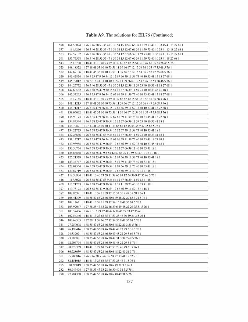
137


578 161,53024 1 76 5 46 28 53 35 47 9 36 54 15 12 67 66 39 11 59 73 40 10 33 45 41 18 27 68 1

577 161,4266 1 76 5 46 28 53 35 47 9 36 54 15 12 67 66 39 11 59 73 40 10 33 41 13 18 27 68 1

563 157,57102 1 76 5 46 28 53 35 47 9 36 54 12 67 66 39 11 59 73 40 10 33 45 41 13 18 27 68 1

561 155,75568 1 76 5 46 28 53 35 47 9 36 54 15 12 67 66 39 11 59 73 40 10 33 41 18 27 68 1

543 153,6788 1 18 41 33 10 40 73 59 11 39 66 67 12 15 54 36 9 47 68 35 53 28 46 5 76 1

523 148,18322 1 27 18 41 33 10 40 73 59 11 39 66 67 12 15 54 36 9 53 47 35 68 5 76 1

522 147,69106 1 18 41 45 33 10 40 73 59 11 39 66 67 12 15 54 36 9 53 47 35 68 5 76 1

520 146,42824 1 76 5 35 47 9 36 54 15 12 67 66 39 11 59 73 40 10 33 41 13 18 27 68 1

519 145,79012 1 68 27 18 41 33 10 40 73 59 11 39 66 67 12 54 8 47 35 53 28 46 5 76 1

515 144,25772 1 76 5 46 28 53 35 47 9 36 54 15 12 39 11 59 73 40 10 33 41 18 27 68 1

508 142,60562 1 76 5 68 35 47 9 20 15 54 12 67 66 39 11 59 73 40 10 33 45 41 18 1

506 142,57265 1 76 5 35 47 9 36 54 12 67 66 39 11 59 73 40 10 33 45 41 13 18 27 68 1

505 141,9165 1 18 41 33 10 40 73 59 11 39 66 67 12 15 54 36 9 53 47 35 68 5 76 1

504 141,11215 1 27 18 41 33 10 40 73 59 11 39 66 67 12 15 54 36 9 47 35 68 5 76 1

500 138,71217 1 76 5 35 47 9 36 54 15 12 67 66 39 11 59 73 40 10 33 41 13 27 68 1

491 138,06092 1 18 41 45 33 10 40 73 59 11 39 66 67 12 54 36 9 53 47 35 68 5 76 1

490 136,90173 1 76 5 35 47 9 36 54 12 67 66 39 11 59 73 40 10 33 45 41 18 27 68 1

486 134,84544 1 76 5 68 35 47 9 36 54 15 12 67 66 39 11 59 73 40 10 33 41 18 1

478 134,72891 1 27 13 41 33 10 40 11 39 66 67 12 15 54 36 9 47 35 68 5 76 1

477 134,22723 1 76 5 68 35 47 9 36 54 15 12 67 39 11 59 73 40 10 33 41 18 1

474 132,28636 1 76 5 68 35 47 53 9 36 54 12 67 66 39 11 59 73 40 10 33 41 18 1

473 131,12717 1 76 5 35 47 9 36 54 12 67 66 39 11 59 73 40 10 33 41 18 27 68 1

472 130,98985 1 76 5 68 35 47 9 36 54 12 67 66 39 11 59 73 40 10 33 45 41 18 1

464 130,50734 1 76 5 68 35 47 9 36 54 15 12 67 66 39 11 40 10 33 41 18 1

460 128,88868 1 76 5 68 35 47 9 8 54 12 67 66 39 11 59 73 40 10 33 41 18 1

455 125,21529 1 76 5 68 35 47 9 36 54 12 67 66 39 11 59 73 40 10 33 41 18 1

440 123,34747 1 76 5 68 35 47 9 36 54 15 12 39 11 59 73 40 10 33 41 18 1

434 122,02554 1 76 5 68 35 47 9 36 54 12 67 66 39 11 73 40 10 33 41 18 1

433 120,87719 1 76 5 68 35 47 9 36 54 12 67 66 39 11 40 10 33 41 18 1

427 119,30904 1 18 41 10 40 73 59 11 39 66 67 12 54 36 9 47 35 68 5 76 1

416 117,8028 1 76 5 68 35 47 53 9 36 54 12 67 66 39 11 59 13 41 18 1

409 113,71733 1 76 5 68 35 47 9 36 54 12 39 11 59 73 40 10 33 41 18 1

397 110,73173 1 76 5 68 35 47 9 36 54 12 67 66 39 11 59 13 41 18 1

382 108,86391 1 18 41 13 59 11 39 12 15 54 36 9 47 35 68 5 76 1

379 108,41309 1 68 35 47 53 28 46 30 6 49 48 22 29 63 3 31 5 76 1

372 108,12621 1 18 41 13 59 11 39 12 54 15 9 47 35 68 5 76 1

363 105,99047 1 27 68 35 47 53 28 46 30 6 49 48 22 29 75 31 5 76 1

361 103,57456 1 76 5 31 3 29 22 48 49 6 30 46 28 53 47 35 68 1

351 102,54346 1 18 41 13 27 68 35 47 53 28 46 30 49 31 3 5 76 1

346 100,68505 1 27 59 11 39 66 67 12 54 36 9 47 35 68 5 76 1

341 97,250008 1 68 35 47 53 28 46 30 6 48 22 29 3 31 5 76 1

340 96,198416 1 68 35 47 53 28 46 30 49 48 22 29 3 31 5 76 1

328 94,539091 1 68 35 47 53 28 46 30 49 48 22 29 3 69 5 76 1

320 93,285881 1 68 35 47 53 28 46 30 49 31 3 34 7 69 5 76 1

318 92,706794 1 68 35 47 53 28 46 30 49 48 22 29 3 5 76 1

312 90,379369 1 18 41 13 27 68 35 47 53 28 46 49 31 5 76 1

306 86,728639 1 68 35 47 53 28 46 30 6 48 22 49 31 5 76 1

301 85,903816 1 76 5 46 28 53 47 35 68 27 13 41 18 52 7 1

292 82,151015 1 18 41 13 27 68 35 47 53 28 46 31 5 76 1

285 81,96819 1 68 35 47 53 28 46 30 6 49 31 3 5 76 1

282 80,946494 1 27 68 35 47 53 28 46 30 49 31 3 5 76 1

278 77,784368 1 68 35 47 53 28 46 30 6 48 49 31 5 76 1

138


274 76,42434 1 68 35 47 53 28 46 30 49 31 3 69 5 76 1

270 71,94028 1 76 5 46 28 53 47 35 68 27 13 41 18 1

254 70,735711 1 76 5 46 28 53 47 35 68 27 41 18 1

241 66,54027 1 68 35 47 53 28 46 31 3 69 5 76 1

238 64,083665 1 68 35 47 53 28 46 30 49 31 5 76 1

232 63,829816 1 18 41 13 27 68 35 47 53 5 76 1

227 63,781461 1 27 68 35 47 9 53 28 46 5 69 76 1

225 62,427949 1 68 35 47 53 28 46 49 31 5 76 1

223 60,554046 1 27 68 35 47 53 28 46 31 5 76 1

218 59,609473 1 68 35 47 53 28 46 30 31 5 76 1

214 56,956328 1 27 68 35 47 53 28 30 46 5 76 1

211 56,710393 1 27 68 35 47 53 28 46 5 69 76 1

205 54,199594 1 68 35 47 53 28 46 31 5 76 1

201 50,343312 1 27 68 35 47 53 28 46 5 76 1

184 48,761354 1 27 68 35 47 53 46 5 76 1

183 43,98886 1 68 35 47 53 28 46 5 76 1

166 42,406902 1 68 35 47 53 46 5 76 1

164 42,367627 1 68 47 53 28 46 5 76 1

163 42,232847 1 27 68 35 47 53 5 76 1

162 40,564544 1 68 35 47 53 28 5 76 1

147 39,077465 1 68 47 35 46 5 76 1

145 35,878395 1 68 35 47 53 5 76 1

144 35,431917 1 27 68 47 35 5 76 1

126 29,077465 1 68 47 35 5 76 1

107 28,989874 1 76 5 47 68 1

106 27,763368 1 5 35 47 68 1

99 26,226562 1 76 5 35 68 1

80 20,77033 1 76 5 68 1

60 19,456233 1 68 5 1

50 15,456233 1 76 5 1

30 10,77033 1 68 1

20 6 1 76 1

The Biobjective TSP with Profit - Middle East Technical ...etd.lib.metu.edu.tr/upload/12608890/index.pdfTHE BIOBJECTIVE TRAVELING SALESMAN PROBLEM WITH ... Kar Getiren GSP, ... Illustration

Documents