Int. J. Nonlinear Anal. Appl. 12 (2021) No. 2, 1083-1097 ISSN: 2008-6822 (electronic) http://www.ijnaa.semnan.ac.ir The Awareness Effect of The Dynamical Behavior of SIS Epidemic Model with Crowley-Martin Incidence Rate and Holling Type III Treatment Function Ahmed A. Mohsen a , Hassan F. AL-Husseiny b,* , Khalid Hattaf c,d a Ministry of Education, Rusafa/1, Baghdad, Iraq. b Department of Mathematics, College of Science, University of Baghdad, Iraq. c Centre Regional desMetiers de l’Education et de la Formation (CRMEF), 20340 Derb Ghalef, Casablanca, Morocco. d Laboratory of Analysis, Modeling and Simulation (LAMS), Faculty of Sciences Ben M’sik, Hassan II University of Casablanca, P.O Box 7955 Sidi Othman, Casablanca, Morocco. (Communicated by Madjid Eshaghi Gordji) Abstract This article deals with the dynamical behaviors for a biological model of epidemic diseases with holling type III treatment function. A Crowley-Martin formula to transmission of disease with coverage media programs effect on the population are introduced and investigated. Through some basic analyses, an explicit formula for the basic reproduction number of the model is calculated, and some results such as the stability analysis and instability of all equilibrium points for the model are established. The local bifurcation occurs near all equilibrium points for the model under some special cases that are studied. The numerical simulations are executed to confirm the theoretical results. Keywords: Infection Diseases, Treatment Function, Awareness Programs, Local Bifurcation, Crowley-Martin formula. 1. Introduction Since the early twentieth century, researchers have designed many epidemiological models that play a fundamental role in understanding the spread of infectious diseases and drawing appropriate and emergency planning to control their spread and reduce risks by developing appropriate policies. * Corresponding author Email addresses: [email protected] (Ahmed A. Mohsen), [email protected] (Hassan F. AL-Husseiny), [email protected] (Khalid Hattaf) Received: May 2021 Revised: June 2021

Welcome message from author
This document is posted to help you gain knowledge. Please leave a comment to let me know what you think about it! Share it to your friends and learn new things together.
Transcript
Int. J. Nonlinear Anal. Appl. 12 (2021) No. 2, 1083-1097ISSN: 2008-6822 (electronic)http://www.ijnaa.semnan.ac.ir
The Awareness Effect of The Dynamical Behavior ofSIS Epidemic Model with Crowley-Martin IncidenceRate and Holling Type III Treatment Function
Ahmed A. Mohsena, Hassan F. AL-Husseinyb,∗, Khalid Hattafc,d
aMinistry of Education, Rusafa/1, Baghdad, Iraq.bDepartment of Mathematics, College of Science, University of Baghdad, Iraq.cCentre Regional desMetiers de l’Education et de la Formation (CRMEF), 20340 Derb Ghalef, Casablanca, Morocco.dLaboratory of Analysis, Modeling and Simulation (LAMS), Faculty of Sciences Ben M’sik, Hassan II University ofCasablanca, P.O Box 7955 Sidi Othman, Casablanca, Morocco.
(Communicated by Madjid Eshaghi Gordji)
Abstract
This article deals with the dynamical behaviors for a biological model of epidemic diseases withholling type III treatment function. A Crowley-Martin formula to transmission of disease withcoverage media programs effect on the population are introduced and investigated. Through somebasic analyses, an explicit formula for the basic reproduction number of the model is calculated, andsome results such as the stability analysis and instability of all equilibrium points for the model areestablished. The local bifurcation occurs near all equilibrium points for the model under some specialcases that are studied. The numerical simulations are executed to confirm the theoretical results.
Keywords: Infection Diseases, Treatment Function, Awareness Programs, Local Bifurcation,Crowley-Martin formula.
1. Introduction
Since the early twentieth century, researchers have designed many epidemiological models thatplay a fundamental role in understanding the spread of infectious diseases and drawing appropriateand emergency planning to control their spread and reduce risks by developing appropriate policies.
∗Corresponding authorEmail addresses: [email protected] (Ahmed A. Mohsen), [email protected]
(Hassan F. AL-Husseiny), [email protected] (Khalid Hattaf)
Received: May 2021 Revised: June 2021

1084 Mohsen, AL-Husseiny, Hattaf
Therefore, mathematical models have become important and essential tools in facing the challengesfacing public health [7, 13, 5, 11]. In recent years, there has been an evolution in mathematicalmodels that have become concerned with studying important factors that help reduce the spreadof diseases and control them such as (treatment, vaccination, disease transmission mechanism andawareness programs), [6, 18].
The vaccine rate is defined a product that stimulates a person’s immune system to produceimmunity to a specific disease, protecting the person from that disease and the treatment rate isdefined a crucial part to reduce the spread of epidemic diseases. While, The incidence rate ortransmission rate of disease is defined as the number of infected individuals per unit time as (hours,days, weeks, month or year). The definition of awareness programs is program designed to increaseawareness of a diseases or anything for more inform [7-14]. Moreover, there are more than oneformula for both incidence rate and treatment such as Kumar et al. [8], proposed SEIR epidemicmodel with nonlinear incidence and treatment rates. Kumar and Nilam introduced SIR epidemicmodel with delay involving Crowley-Martin type incidence rate [9]. Yang and Wei studied andanalyzed mathematical model for epidemic disease with Crowley-Martin incidence rate and treatmenteffects[20]. Adnani et al. studied stability analysis of SIR epidemic model with specific nonlinearincidence rate [1]. Dubey et al. [4], suggested SIR model with nonlinear incidence rate and treatmentfunction.
In this study, we are aiming to analyze an epidemic diseases dynamical model of SIS type with aCrowley-Martin incidence rate and holling type III treatment function. This incidence function willcover a variety of incidence functions presented in all the studies cited previously. Another importantfeature of our model is the fact that we include also awareness effect by the media coverage to reduceand control of the diseases spread such as [15, 12]. On the other hand, we discuss the changesin dynamic behavior or so-called bifurcation that received great attention due to they have beenobserved in the incidence of many infectious diseases. Hence, The rest of this work is outlined asfollows. In the next section, we will discuss the well posed of the proposeded model by confirmingthe existence, positivity and boundedness of solutions. In Section 3, we present an analysis of themodel such as calculate the basic reproduction number of this model and equilibrium points. InSections 4,5, we prove the stability analysis of the all equilibrium points. In Section 6, we discussthe local bifurcation accrue near all the equilibrium points. Finally, numerical simulations are givenin Section 7, to confirm the analytic results and the comparison with the numerical results.
2. Model formulation and basic properties
2.1. Model formulation
We develop and formulate a biological mathematical model by nonlinear ordinary differentialequations in this section. This model describes of an infectious disease of SIS type in the population.To understand the dynamical behavior of the proposed model we assume that the population isdivided into three compartments are: the all susceptible individuals and unawareness of the diseaseS(t), the individuals who have awareness of the disease Sa(t), the all infected individuals I(t), themedia programs for awareness denoted by M(t). The way disease transmission is direct contactthrough nonlinear function. Finally, the infected individuals can treat them with a type III function.

The Awareness Effect of The Dynamical Behavior ... 12 (2021) No. 2, 1083-1097 1085
All the above hypotheses can be written as below
dS
dt= ψ − γSM − βSI
(1 + αS)(1 + θI)+
a1I2
1 + b1I2− µS,
dSadt
= γSM − µSa,
dI
dt=
βSI
(1 + αS)(1 + θI)− a1I
2
1 + b1I2− µI,
dM
dt= ρS − σM,
(2.1)
with the initial conditions S (0) > 0; Sa (0) > 0; I (0) ≥ 0 ,M(0) > 0.All the parameters in the propose model are positive. The birth rate in the population is ψ, the
transmission rate of disease is β with α is a measure of inhibition effect, such as preventive measuretaken by susceptible individuals and θ is a measure of inhibition effect such as treatment with respectto infective, the term a1I2
1+b1I2represented to treatment function such that a1 is treatment rate and b1
is limitation rate in treatment availability, the death rate is µ, the media rate represented by γ, theimplementation rate of media campaigns is denoted by ρ and diminishing rate is represented by θ .
2.2. Boundedness
Theorem 2.1. The uniformly bounded of the any solutions are discussion in the following.Proof . Let (S(t), Sa(t), I(t),M(t)) is the solution of the model (2.1) with positive initial condition(S(0), Sa(0), I(0),M(0)), we assume that
N(t) = S(t) + Sa(t) + I(t),
by the derivative of N(t) along the solution of the model (2.1), this gives
dN
dt= ψ − µ(S + Sa + I),
dN
dt≤ −µN.
(2.2)
which implies that
limt→∞
supN(t) ≤ ψ
µ. (2.3)
while, the last equation of system (2.1) it follows that
dM
dt≤ ρS − σM,
M(t) ≤ ρ
σ.
(2.4)
By similar way we get:
M(t) ≤ ρψ
σµ, as t→∞. (2.5)
We obtain that, the solution of model (2.1) are confined in the following region
Ω =
(S, Sa, I,M)?R4
+ : N ≤ ψ
µ, 0 ≤M ≤ ρψ
σµ
. (2.6)
Clearly, we have any solutions of model (2.1) are uniformly bounded.

1086 Mohsen, AL-Husseiny, Hattaf
3. The Number of Equilibria Points
obviously, the aware susceptible Sa is related with variables S(t) and M(t) only. Hence for findvalues of, S(t) and M(t), the calculate value of Sa can be found simply by solving the model (2.1).In fact, we can determine the value of Sa by the following equation
Sa =γSM
1 + µ. (3.1)
Consequently, we can reduced system (2.1) and rewrite it to the following system
dS
dt= ψ − γSM − βSI
(1 + αS)(1 + θI)+
a1I2
1 + b1I2− µS,
dI
dt=
βSI
(1 + αS)(1 + θI)− a1I
2
1 + b1I2− µI,
dM
dt= ρS − σM.
(3.2)
Now, we can computing the reproduction number for the given system (3.2) and denoted by R0, suchthat
R0 =βS0
µ(1 + αS0). (3.3)
Therefore, system (3.2) has at most two biologically feasible points, namely, Ei = (Si, Ii,Mi), i = 0, 1.The existence conditions for each of these equilibrium points are discussed in following:
• The first equilibrium point is exist when I = 0 , and called disease free steady state whichdenoted by E0 = (S0, 0,M0), where
M0 =ρ
σS0. (3.4)
As well as, S0 is a positive through the following quadratic equation
A1S20 + A2S0 + A3 = 0. (3.5)
Such that
S0 =−(A2 +
√A2
2 − 4A1A3)
2A1
,
A1 =−γρσ
,
A2 = −µ,A3 = ψ.
(3.6)
• The endemic steady state, denoted by E1 = (S1, I1,M1) such that
M1 =ρ
σS1. (3.7)
While (S1, I1) represents a positive intersection point of the following two isocline:
f(S, I) = r1S3 + r2S
3I3 + r3S3I2 + r4S
3I + r5S2 + r6S
2I3 + r7S2I2 + r8S
2I
+ r9S + r10SI3 + r11SI
2 + r12SI + r13I3 + r14I
2 + r15I + r16 = 0(3.8)

The Awareness Effect of The Dynamical Behavior ... 12 (2021) No. 2, 1083-1097 1087
g(S, I) = q1SI3 + q2I
3 + q3SI2 + q4I
2 + q5SI + q6I + q7S + q8 = 0. (3.9)
Here,
r1 = −γρα, r2 = −γραθb1, r3 = −γραb1,
r4 = −γραθ, r5 = −(γρ+ µσα), r6 = −(γρθb1 + µσαθb1),
r7 = −(γρb1 + µσαb1), r8 = −(γρθ + µσαθ), r9 = (ψσα− µσ),
r10 = (ψσαθb1 − βσb1 + a1σαθ − µσθb1) r11 = (ψσθb1 + a1σα− µσb1), r12 = (ψσαθ − βσ − µσθ),r13 = (ψσθb1 + a1σθ), r14 = (ψσb1 + a1σ), r15 = ψσθ,
r16 = ψσ, q1 = −µαθb1, q2 = −µb2,
q3 = (βb1 − a1αθ − µαb1), q4 = −(a1θ + µb1), q5 = −(a1α + µαθ),
q6 = −(a1 − µθ), q7 = (β − µα), q8 = −µ
It easy, when I → 0, we get the equations (3.8) and (3.9) becomes as follows
f(S) = r1S3 + r5S
2 + r9S + r16 = 0, (3.10)
g(S) = q7S + q8 = 0. (3.11)
Obviously, by using Descartes rule equation (3.10) has a unique positive root S. However,equation (3.11), has a positive root S = −q8
q7. Then, the equations (3.8) and (3.9) have a unique
positive root and the endemic equilibrium point E1 exists if the following conditions are satisfy
α < min
µ
ψ,β
µ
,
S < S
∂I
∂S= −
∂f∂S∂f∂I
> 0,
∂I
∂S= −
∂g∂S∂g∂I
< 0.
(3.12)
4. Local dynamical behavior
In this section, the stability analysis investigation of model (3.2) about Ei, i = 0, 1 are studied inthe following theorems.
Theorem 4.1. The disease free equilibrium point E0 of the system (3.2) is locally stable underR0 < 1.Proof .From the linearization method of system (3.2) about E0 we have
J(E0) =
−γM0 − µ −βS0
(1+αS0)−γS0
0 βS0
(1+αS0)− µ 0
ρ 0 −σ
(4.1)
Therefore the characteristic equation is[(βS0
(1 + αS0)− µ
)− λ] [λ2 + A1λ+ A2
]= 0. (4.2)

1088 Mohsen, AL-Husseiny, Hattaf
Here,A1 = γM0 + µ+ σ, A2 = (γM0 + µ)σ + γρS0. (4.3)
Consequently the eigenvalues of equation (4.2) can be written in below
λI =βS0
(1 + αS0)− µ ,
λs = −A1
2+
1
2
√A2
1 − 4A2 ,
λµ = −A1
2− 1
2
√A2
1 − 4A2 ,
(4.4)
Therefore, all the eigenvalues have negative real part and hence the disease-free equilibrium pointis locally stable in case R0 < 1.
Theorem 4.2. The local stability about E1 of system (3.2) is guarantee when R0 > 1 and thefollowing sufficient conditions
βs1
(1 + αs1)(1 + θI1)2<2a1I1
(1 + b1I21 )2
, (4.5)[−βs1
(1 + αs1)(1 + θI1)2+2a1I1
(1 + b1I21 )2
] [βI1
(1 + θI1)(1 + αs1)2
]< ργs1. (4.6)
Proof . From the linearization method of system (3.2) about E1 we have
J(E1) =
−γM1 − βI1(1+θI1)(1+αs1)2
− µ −βs1(1+αs1)(1+θI1)2
+ 2a1I1(1+b1I21 )2
−γs1
βI1(1+θI1)(1+αs1)2
βs1(1+αs1)(1+θI1)2
− 2a1I1(1+b1I21 )2
− µ 0
ρ 0 −σ
(4.7)
The characteristic equation is given by;
λ3 +B1λ2 +B2λ+B3 = 0. (4.8)
Here
B1 = −(b11 + b22 + b33),
B2 = b11b22 − b12b21 + b11b33 − b13b31 + b22b33,
B3 = −b11b22b33 + b13b22b31 + b12b21b33,
∆ = −b11b22 [b11 + b22]− b11b33 [b11 + b33]− b22b33 [b22 + b33]
− 3b11b22b33 + [b11 + b22 + b33] [b12b21 + b13b31] .
Now, if the conditions of Routh-Hurwitz method (Bi(i = 1, 3) > 0 and ∆ = B1B2 − B3 > 0)aresatisfied. Then, we get the all eigenvalues of J(E1) have negative real part roots. Consequently, theit is locally stable under the conditions (4.5) and (4.6).

The Awareness Effect of The Dynamical Behavior ... 12 (2021) No. 2, 1083-1097 1089
5. Global dynamical behavior
In this section, the region of global dynamical behavoir of all equilibria points of system (3.2) isstudied in below theorems.
Theorem 5.1. The E0 is a globally asymptotically stable when R0 < 1, and provided that the con-ditions in below (
ρ
M− γS0
S
)2
< 4
(γM + µ
S
)( σM
), (5.1a)
β
(1 + αS)(1 + θI)<
a1I
S(1 + b1I2). (5.1b)
Proof . We definite the positive functionW0(S, I,M) = (S − S0 − S0 ln S
S0) + I + (M −M0 −M0 ln M
M0).
Clearly, W0 : R3+ → R is a continuously differentiable function such that W0(S0, 0,M0) = 0 and
W0(S, I,M) > 0,∀(S, I,M) 6= (S0, 0,M0). Further,
dw0
dt= (
S − S0
S)
[ψ − γSM − βSI
(1 + αS)(1 + θI)+ h(I)− µS
]+
[βSI
(1 + αS)(1 + θI)− a1I
2
1 + b1I2− µI
]+ (
M −M0
M) [ρS − σM ]
Now, by doing some algebraic manipulation and using the conditions (5.1a) - (5.1b), we get
dW0
dt≤ −(
γM + µ
S)(S − S0)2 + (
ρ
M− γS0
S)(S − S0)(M −M0)− σ
M(M −M0)2 +
βS0I
(1 + αS)(1 + θI)
− a1S0I2
S(1 + b1I2)− µI.
Consequently, due to condition above dW0
dt< 0. Thus E0 is a globally asymptotically stable under
the conditions (5.1a) and (5.1b).
Theorem 5.2. The E1 is a globally asymptotically stable under R0 > 1, and provided that belowconditions
β(1 + αS1)S
(1 + αS)(1 + θI)(1 + αS1)(1 + θI1)< µ+
a1(I + I1)
(1 + b1I2)(1 + b1I21 ), (5.2)
q212 < 2q11q22, (5.3)
q213 < 2q11q33. (5.4)
Proof . Consider the following positive definite function
W1(S, I,M) =(S − S1)2
2+
(I − I1)2
2+
(M −M1)2
2.
Clearly, W1 : R3+ → R is a continuously differentiable function such that W1(S1, I1,M1) = 0 and
W1(S, I,M) > 0,∀(S, I,M)?R3+ and (S, I,M) 6= (S1, , I1,M1).
Now, by the derivative with respect to system (3.2) we get the resulting

1090 Mohsen, AL-Husseiny, Hattaf
dW1
dt= (S − S1)
[ψ − γSM − βSI
(1 + αS)(1 + θI)+
a1I2
1 + b1I2− µS
]+ (I − I1).[
βSI
(1 + αS)(1 + θI)− a1I
2
1 + b1I2− µI
]+ (M −M1) [ρS − σM ] .
dW1
dt= −
[q11
2(S − S1)2 + q12(S − S1)(I − I1) + q22(I − I1)2
]−[q11
2(S − S1)2 + q13(S − S1)(M −M1) + q33(M −M1)2
]Clearly, by the conditions (5.2)- (5.4) we get that
dW1
dt≤ −
[√q11
2(S − S1) +
√q22(I − I1)
]2
−[√
q11
2(S − S1) +
√q33(M −M1)
]2
.
Such that
q11 = γM +β(1 + θI)I1
(1 + αS)(1 + θI)(1 + αS1)(1 + θI1)+ µ,
q12 =β[(1 + αS1)S − (1 + θI)I1]
(1 + αS)(1 + θI)(1 + αS1)(1 + θI1)− a1(I + I1)
(1 + b1I2)(1 + b1I21 ),
q22 =a1(I + I1)
(1 + b1I2)(1 + b1I21 )
+ µ− β(1 + αS1)S
(1 + αS)(1 + θI)(1 + αS1)(1 + θI1),
q13 = γS1 − ρ, q33 = σ.
It is easy see that, dw1
dt< 0. So, E1 is globally asymptotically stable when the given conditions are
satisfied.
6. The Bifurcation Analysis
In the next theorem the conditions of bifurcation occur of system (2) is established. Mathemati-cally bifurcation of the system means that if the change a parameter value in special cases then thesolution of the system will change according to this parameter for all the time. Now, we can writesystem (3.2) in the formula: dX
dt= F (X), here X = (S, I,M)T such that F = (f1, f2, f3)T while
fi; i = 1, 2, 3 represent to the system (3.2). So according to the jacobian matrix of system (3.2), it iseasy to verify that for any vector V = (v1, v2, v3)T , we have that second directional derivative
D2F (S,C,M)(V, V ) =
2
αβIv21(1+θI)(1+αS)3
− βv1v2(1+θI)2(1+αS)2
− γv1v3 +[
θβS(1+αS)(1+θI)3
+ a1−3a1b1I2
(1+b1I2)3
]v2
2
2
−αβIv21(1+θI)(1+αS)3
+ βv1v2(1+θI)2(1+αS)2
+[
−θβS(1+αS)(1+θI)3
+ 3a1b1I2−a1(1+b1I2)3
]v2
2
0
.(6.1)

The Awareness Effect of The Dynamical Behavior ... 12 (2021) No. 2, 1083-1097 1091
6.1. The Bifurcation condition about E0
Theorem 6.1. If R0 = 1, the transcritical bifurcation can occur at E0 of system (3.2).Proof . The R0 = 1 when the parameter µ ≡ µ∗, thenEq.(4.1)ofsystem(3.2)atE0, has zero eigen-value (λ0 = 0).
µ = µ∗ =βS0
(1 + αS0)≡ R0 = 1. (6.2)
So, Eq.(4.1) of system (3.2) can be represent by
J0 = J0(µ) =
−γM0 − µ −µ −γS0
0 0 0ρ 0 −σ
.Clearly, let V[0] = (v
[0]1 , v
[0]2 , v
[0]3 )T representstheeigenvectorsofJ0 of λ0 = 0.
So(J0 − λ0)V [0] = 0, get that V [0] = (m1v
[0]3 ,m2v
[0]3 , v
[0]3 )T ,
suuch that, m1 = σρ, m2 = − (1+αS0)
βS0
[γS0 + σ(γM0+µ)
ρ
], with v
[0]3 6= 0.
As well as, let L[0] =[l[0]1 , l
[0]2 , l
[0]3
]Trepresents the eigenvectors of λ0 = 0 of JT0 .
Obviously from(JT0 − λ0)L[0] = 0
. We obtain L[0] =[0, l
[0]2 , 0
]T; such that l
[0]2 6= 0 .
Now, consider∂F
∂µ= Fµ(X, β) = [−S,−I, 0]T
Thus, Fµ(E0, µ) = [−S0, 0, 0]T which gives[L[0]]TFµ(E0, µ) = 0.
So, by help of the Sotomyor’s theorem bifurcation theory, the saddle nod bifurcation is not occur nearE0 of system (3.2). Furthermore, because we have
DFµ(X,µ) =
−1 0 00 −1 00 0 0
.We can see that
DFµ(E0, µ)V [0] =
−1 0 00 −1 00 0 0
σρv
[0]3
− (1+αS0)βS0
[γS0 + σ(γM0+µ)
ρ
]v
[0]3
0
6= 0.
Moreover, by substituting E0, µ and V [0] in (31) we get:
D2F (E0, µ)(V [0], V [0]) =2[
αβIm21
(1+θI)(1+αS)3− βm1m2
(1+θI)2(1+αS)− γm1
](v
[0]3 )2 +
[θβS
(1+αS)(1+θI)3+ a1−3a1b1I2
(1+b1I2)3
]m2
2(v[0]3 )3
2[
βm1m2
(1+θI)2(1+αS)2− αβIm2
1
(1+θI)(1+αS)3
]+[
3a1b1I2−a1(1+b1I2)3
− θβS(1+αS)(1+θI)3
]m2
2(v[0]3 )2
0
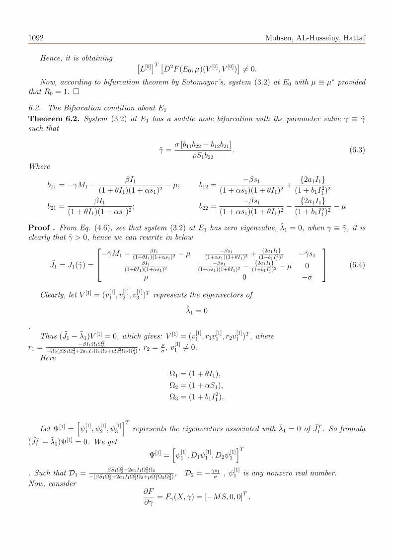
1092 Mohsen, AL-Husseiny, Hattaf
Hence, it is obtaining [L[0]]T [
D2F (E0, µ)(V [0], V [0])]6= 0.
Now, according to bifurcation theorem by Sotomayor’s, system (3.2) at E0 with µ ≡ µ∗ providedthat R0 = 1.
6.2. The Bifurcation condition about E1
Theorem 6.2. System (3.2) at E1 has a saddle node bifurcation with the parameter value γ ≡ γsuch that
γ =σ [b11b22 − b12b21]
ρS1b22
. (6.3)
Where
b11 = −γM1 −βI1
(1 + θI1)(1 + αs1)2− µ; b12 =
−βs1
(1 + αs1)(1 + θI1)2+2a1I1
(1 + b1I21 )2
b21 =βI1
(1 + θI1)(1 + αs1)2; b22 =
−βs1
(1 + αs1)(1 + θI1)2− 2a1I1
(1 + b1I21 )2− µ
Proof . From Eq. (4.6), see that system (3.2) at E1 has zero eigenvalue, λ1 = 0, when γ ≡ γ, it isclearly that γ > 0, hence we can rewrite in below
J1 = J1(γ) =
−γM1 − βI1(1+θI1)(1+αs1)2
− µ −βs1(1+αs1)(1+θI1)2
+ 2a1I1(1+b1I21 )2
−γs1
βI1(1+θI1)(1+αs1)2
−βs1(1+αs1)(1+θI1)2
− 2a1I1(1+b1I21 )2
− µ 0
ρ 0 −σ
(6.4)
Clearly, let V [1] = (v[1]1 , v
[1]2 , v
[1]3 )T represents the eigenvectors of
λ1 = 0
.Thus (J1 − λ1)V [1] = 0, which gives: V [1] = (v
[1]1 , r1v
[1]1 , r2v
[1]1 )T , where
r1 =−βI1Ω1Ω2
3
−Ω2(βS1Ω23+2a1I1Ω1Ω2+µΩ2
1Ω2Ω23)
, r2 = ρσ
, v[1]1 6= 0.
Here
Ω1 = (1 + θI1),
Ω2 = (1 + αS1),
Ω3 = (1 + b1I21 ).
Let Ψ[1] =[ψ
[1]1 , ψ
[1]2 , ψ
[1]3
]Trepresents the eigenvectors associated with λ1 = 0 of JT1 . So fromula
(JT1 − λ1)Ψ[1] = 0. We get
Ψ[1] =[ψ
[1]1 , D1ψ
[1]1 , D2ψ
[1]1
]T. Such that D1 =
βS1Ω23−2a1I1Ω2
1Ω2
−(βS1Ω23+2a1I1Ω2
1Ω2+µΩ21Ω2Ω2
3), D2 = −γs1
σ, ψ
[1]1 is any nonzero real number.
Now, consider∂F
∂γ= Fγ(X, γ) = [−MS, 0, 0]T .

The Awareness Effect of The Dynamical Behavior ... 12 (2021) No. 2, 1083-1097 1093
So, Fγ(E1, γ) = [−M1S1, 0, 0]T and then[Ψ[1]]TFγ(E1, γ) 6= 0.
However, the system (3.2) has no transcritical bifurcation. But the 1st condition of the bifurcationtheorem about saddle-node type is satisfied. Now, since
DFγ(X, γ) =
−M 0 −S0 0 00 0 0
Where DFγ(X, γ) represent the derivative of Fγ(X, γ) with X = [S, I,M ]T . Moreover, it is clearly
DFγ(E1, γ)V [1] =
−M 0 −S0 0 00 0 0
V [1] =
−(M + r2S)v[1]1
00
[Ψ[1]]T [
DFγ(E1, γ)V [1]]
=[ψ
[1]1 , D1ψ
[1]1 , D2ψ
[1]1
]−(M + r2S)v[1]1
00
= −(M + r2S)ψ[1]1 v
[1]1 6= 0.
Moreover, by substituting E1, γ and V [1] in (6.1) we get:
D2F (E1, γ)(V [1], V [1]) =
2(v
[1]1 )2 αβI
(1+θI)(1+αS)3− βr1
(1+θI)2(1+αS)2− γr2 +
[θβS
(1+αS)(1+θI)3+ a1−3a1b1I2
(1+b1I2)3
]r2
1
2(v[1]1 )2 −αβI
(1+θI)(1+αS)3+ βr1
(1+θI)2(1+αS)2+[
−θβS(1+αS)(1+θI)3
+ 3a1b1I2−a1(1+b1I2)3
]r2
10
.Hence, it is obtain
[Ψ[1]]T [
D2F (E1, γ)(V [1], V [1])]6= 0.
Hence, the system (3.2)] has a saddle-node bifurcation at E1 with parameter γ.
7. The numerical illustration of system (2.1)
The global dynamical behavior of system (2.1) will studied numerically for different sets of pa-rameters and different sets of initial points in this section. The goal of such part are know the role ofchange the parameters values and confirm the analytical results. It is see that that, for the followingbiologically feasible set of parameters values:
ψ = 50, γ = 0.01, β = 0.25, α = 0.05, θ = 0.1,
a1 = 0.3, b1 = 0.05, µ = 0.4, ρ = 0.4, σ = 0.3(7.1)
The trajectory of system (2.1) convergent to E1 see Fig.(1).

1094 Mohsen, AL-Husseiny, Hattaf
Figure 1: Time attractor of globally asymptotically stable to E1 of system (2.1) and R0 = 4.61 > 1.
However, for the data by equation (7.1) with β = 0.025 the trajectory of system (2.1) convergentto E0 see Fig. (2).

The Awareness Effect of The Dynamical Behavior ... 12 (2021) No. 2, 1083-1097 1095
Figure 2: Time attractor of globally asymptotically stable to E0 of system (2.1) and R0 = 0.46 < 1.
Clearly, in order to discuss the impact of varying some parameter values on the dynamical behaviorof system (2.1), the following results are observed. According to the Fig.3, it is clear that thetrajectory of system (2.1) convergent to E0 by applied the parameters values given in Eq. (7.1) withvaryingα > 0.5 with R0 = 0.79 < 1.
Figure 3: The measure of inhibition effect on the dynamical behavior of system (2.1).
Also we applied the parameters values given in Eq. (7.1) but putting µ ≥ 2.6 the trajctory of thesystem (2.1) convergent to E0 = (17.635, 1.595, 0, 23.514) and R0 = 0.65 < 1, see Fig.(4) below.

1096 Mohsen, AL-Husseiny, Hattaf
Figure 4: The death rate effect on the dynamical behavior of system (2.1).
Now, the effect of media coverage is discussion by Fig. 5, it easy see that when the level ofawareness increasing due to the media coverage (say γ), we obtain the dynamical behavior of system(2.1) convergent to E0 and that is mean the endemic equilibrium point becomes unstable whenγ ≥ 0.6. In addition we get similar result if the media rate increasing through ρ ≥ 20.
Figure 5: The response effect to media programs on the dynamical behavior of system (2.1).
8. Conclusion and Results
In this study, we have examined the epidemic model with SIS type under the effect of mediaprograms, the Crowley-Martin formula to transmission of disease and holling type III treatmentfunction. We have also provided the existence of all equilibrium points and calculated the basicreproduction number. The local stability results studied by applying the trace-determinant andRouth-Hurwitz Criterion. As well as, the global stability results studied by applying the techniqueand theorem of the Lyapunov function. In addition, we investigated the local bifurcation suchas (transcritical, saddle node and pitchfork bifurcation) around all the equilibrium points of the

The Awareness Effect of The Dynamical Behavior ... 12 (2021) No. 2, 1083-1097 1097
proposed model according to Sotomayor’s theorem. Through the numerical simulation, we confirmthe analytical results that have been interpreted through graphical representation. The graphicrepresentation provides rich details to the global health through which mathematical models can bean important factor in understanding the behavior of epidemic disease spread and control.
References
[1] J. Adnani, K. Hattaf and N. Yousfi, Stability analysis of a stochastic SIR epidemic model with specific nonlinearincidence rate, (2013)1-4 article ID 431257.
[2] R. M. Anderson, R. M. May, Infectious Diseases of Humans: Dynamics and Control, Oxford University Press,New York (1992).
[3] N. T. Bailey, etal., The mathematical theory of infectious diseases and its applications, Charles Griffin & CompanyLtd, 5a Crendon Street, High Wycombe, Bucks HP13 6LE.(1975).
[4] P. Dubey, B. Dubey and S. Dubey, An SIR model with nonlinear incidence rate and holling type III treatmentrate, Applied Analysis in Bioloical and Physical Sciences, 186 (2016) 63-81.
[5] I. M. Foppa, A historical introduction to mathematical modeling of infectious diseases, Elsevier Inc., (2017).[6] J. M. Hyman and J. Li, Modeling the effectiveness of isolation strategies in preventing STD epidemics, SIAM J.
Appl. Math. 3 (1998) 912-925.[7] M. Keeling and P. Rohani, Modeling Infectious Diseases in Humans and Animals, Princeton University Press.
(2008).[8] R. Kumar, A. Kumar, S. Kumari and P. Roy, Dynamic of an SEIR epidemic model with nonlinear incidence
and treatment rates, Nonlinear Dyn., 96 (2019) 2351-2368.[9] A. Kumar and Nilam, Dynamic Behavior of an SIR Epidemic Model along with Time Delay; Crowley-Martin Type
Incidence Rate and Holling Type II Treatment Rate, International Journal of Nonlinear Sciences and NumericalSimulation, 20 (2019) 757-771.
[10] L. Li, Y. Bai, Z. Jin, Periodic solutions of an epidemic model with saturated treatment, Nonlinear Dyn. 2 (2014)1099-1108.
[11] M. Li, An introduction to Mathematical Modeling of Infectious Diseases, Springer International publishing. (2018).[12] M. Ibrahim, M. Kamran, M. Naeem, S. Kim and H. Jung, Impact of awareness to control malaria disease: a
mathematical modeling approach, Complexity, Article ID 8657410. (2020) 1-13.[13] Z. Ma and J. Li, Dynamical Modeling and Analysis of Epidemics, World scientific publishing. (2009).[14] A. Mohsen, Bifurcation analysis in simple SIS epidemic model involving immigrations with treatment, Appl.
Math. Inf. Sci. Lett. 3 (2015) 97-102.[15] A. Mohsen, H. AL-Husseiny, X. Zhou and K. Hattaf, Global stability of COVID-19 model involving the quarantine
strategy and media coverage effects, AIMS Public Health, 3 (2020) 587-605. doi: 10.3934/publichealth.2020047.[16] R. Naji and A. Mohsen, Stability analysis with bifurcation of an SVIR epidemic model involving immigrants,
Iraqi journal of Science. 54 (2013) 397-408.[17] https://www.cdc.gov/vaccines/vac-gen/imz-basics.htm.[18] L. I. Wu and Z. Feng, Homoclinic bifurcation in an SIQR model for childhood diseases, J. Differ. Equ. 1 (2000)
150-167.[19] R. Xu and Z. Ma, Global stability of a delayed SEIRS epidemic model with saturation incidence rate. Nonlinear
Dyn, 61 (2010) 229-239.[20] L. Yang and F. Wei, Analysis of an epidemic model with Crowley-Martin incidence rate and holling type II
treatment, Ann. Of Appl. Math., 36 (2020) 204-220.[21] X. Zhou, J. Cui, Analysis of stability and bifurcation for an SEIV epidemic model with vaccination and nonlinear
incidence rate, Nonlinear Dyn. 4 (2011) 639-653.
Related Documents