THE ARYABHATA PROJECT Edited by U. R, RAO, K. KASTURIRANGAN - ! - .’ j: ||)| if ijj} ' ' fpfjf- INDIAN ACADEMY OF SCIENCES Bangalore 660 006

Welcome message from author
This document is posted to help you gain knowledge. Please leave a comment to let me know what you think about it! Share it to your friends and learn new things together.
Transcript

THE ARYABHATA PROJECT
Edited by
U. R, RAO, K. KASTURIRANGAN
- ! - .’ j: ||)| if ijj} ' ' fpfjf-
INDIAN ACADEMY OF SCIENCES
Bangalore 660 006


Digitized by the Internet Archive in 2018 with funding from
Public.Resource.Org
https://archive.org/details/aryabhataprojectOOunse

THE ARYABHATA PROJECT
Edited by
U. R. RAO, K. KASTURIRANGAN ISRO Satellite Centre, Bangalore
INDIAN ACADEMY OF SCIENCES
Bangalore 560 006

© 1979 by the Indian Academy of Sciences
Reprinted from the Proceedings of the Indian Academy of Sciences, Section C: Engineering Sciences, Volume 1, pp. 117-343, 1978
Edited by U R Rao, K Kasturirangan and printed for the Indian Academy of Sciences by Macmillan India Press, Madras 600 002, India

Foreword
Space exploration and space travel have been the dream of mankind since early ages. When the first sputnik was launched into space in 1957 by USSR, the entire world was dramatically ushered into the space age. With the remarkable develop¬ ments that have taken place in space sciences and technology during the last two decades, some of mankind’s wildest dreams and visions—such as men walking on the moon, close-up pictures of Venus, Mars and Jupiter, in-situ exploration of planets, space docking near earth, space shuttle transportation—have all come true. The space era has opened up new windows into the skies, enabling scientists to obtain a view of the universe in X-rays and in ultraviolet, infrared and gamma rays, which had been inaccessible earlier. Developments in space technology now offer unique plat¬ forms to carry out remote sensing of our natural resources and unearth new ones in agriculture, forestry, mineralogy, hydrology, oceanography, geography and even cartography. Mass communication and meteorological observation on a global scale have now become a practical reality with geosynchronous satellites. Thus, space science and technology seem to offer a new hope for improving the quality of life on earth.
Based on the firm belief that through purposeful, selective and imaginative utili¬ sation of space technology, it is possible to provide unique inputs into the process of national development, the Indian Space Research Organisation (ISRO) entered into an agreement in 1972 with the USSR Academy of Sciences for launching the first Indian Satellite from a Soviet cosmodrome. With the launching of this satellite, the Aryabhata, on 19 April 1975, into a near-earth circular orbit at a height of 600 km, India entered the space age. The primary aim of Aryabhata was to establish the neces¬ sary expertise and infrastructure in satellite technology. Even though the original estimated life of Aryabhata was only 6 months, all the technological systems on the satellite have been functioning satisfactorily for the last three and half years.
This volume, comprising two special issues of the Academy’s Proceedings on Arya¬ bhata, contains various articles on the technological design of the spacecraft, and is the outcome of the keen interest taken by the Academy to publish a technical account of the project. In particular, the keen interest taken by Prof. S Dhawan, the President of the Academy, and Prof. R Narasimha, Editor for Engineering Sciences has been an important factor, without which these issues could not have been published. We are thankful to all the authors of various articles who have responded enthusiastically in providing the articles in time. The Editors are grateful to Dr P N Pathak, Mr V Kalayan Raman, Dr V Siddhartha and Dr Esther Ramani who provided very valuable assistance in editing the papers appearing in this special issue.
U R RAO K KASTURIRANGAN Editors

'
■
’

CONTENTS
Foreword
U R RAO: An overview of the Aryabhata project 1
P S GOEL, P N SRINtVASAN and N K MALIK: The stabilisation system 19
S Y RAMAKRISHNAN, R S MATH U R, M SUBRAMANIAN, T KANTHI-
MATH1NATHAN, SUDARSHAN SARPANGAL, S T VENKATA-
RAMANAN and N S SAVALGI: The power system 29
H N MURTHY, V K KAILA, V PRASAD, D R BHANDARI, H BHOJA-
RAJ and P P GUPTA: The thermal control system 41
G A KASIVISWANATHAN, V P V VARADARAJULU, P R VENKATES-
WARAN and T K ALEX: Attitude and temperature sensors 57
D V RAJU, R K RAJANGAM, P S RAJYALAKSHMI, C N VENKATE-
SHAIAH, R SESHAIAH, V NALANDA, S R NAGARAJ and R SIVA-
SWAMY: The telemetry system 69
M K SAHA, V GOPAL RAO, N MANTHIAH, S KALYANARAMAN,
M L N SASTRY, D JOHN and M K NAIR: The communication system 79
R ASHtYA, J P GUPTA, Y K S1NGAL, D VENKATARAMANA, A BHAS-
KARANARAYANA, U N DAS and B V SESHADRI: The tele¬
command system 89
S P KOSTA, S PAL, P K REDDY, V K LAKSHMEESHA, K N S RAO,
K N SHAMANNA, V MAHADEVAN. V S RAO and L NICHOLAS:
Antenna systems for the Aryabhata mission 105
M K SAHA, S KALYANARAMAN, S N PRASAD, R N TYAGI,
T K JAYARAMAN, M SAMBASIVA RAO and S G BASU: The
tracking system 119
A V PATKI: The structure 135
V A THOMAS, M N SATHYANARAYAN, V R KATTI, A A BOKIL,
N R DATHATHRI, G MOH ANAKRISHNAN, K PATTABHIRAMAN,
T K GOSWAMI, T L DANABALAN and I SELVARAJ: System
integration 151
TARSEM SINGH, A D DHARMA, O P SAPRA. V R PRATAP,
K A NARAYANAN, S SUBBIAH, J V INGLE, A S BHAMAVATI
and B K SHAMAPRAKASH: The ground checkout system 163
R S BHAT and C K RAJASINGH: Orbit computations 175
P N PATHAK: A statistical analysis of weight and cost parameters of space¬
craft with special reference to Aryabhata 1$7

VI Contents
M V K APPA RAO, S V DAMLE, R R DANIEL, G S GOKHALE,
GEORGE JOSEPH, R U KUNDAPURKAR and P J LAVAKARE:
An experiment to detect energetic neutrons and gamma rays from the sun 197
S PRAKASH, B H SUBBARAYA, V KUMAR, P N PAREEK,
J S SHIRKE, R N MISRA, K K GOSWAMI, R S SINGH and
A BANERJEE: The aeronomy experiment 205
U R RAO, K KASTURIRANGAN, Y K JAIN, ARUN BATRA, V JAYA-
RAMAN, R A GANAGE, D P SHARMA and M S RADHA: The x-ray
astronomy experiment 215
Author index 299
Subject index 233
An overview of the 4 Aryabhata ’ project
UR RAO ISRO Satellite Centre, Peenya, Bangalore 560 058
MS received 29 October 1977; revised 10 March 1978
Abstract. Aryabhata, India’s first satellite, was successfully launched into a near- earth orbit on 19 April 1975, from a USSR Cosmodrome. The primary objective of Aryabhata was to establish the indigenous capability in satellite technology. Aryabhata, weighing 358 kg, was quasispherical in shape, and had body-mounted solar cells and Ni-Cd chemical batteries as primary power sources. Other features of the spacecraft include power control systems, passive thermal control system, PCM/FM/PM telemetry system transmitting data at 256 bits/s in real time and 2560 bits/s in the stored mode, PDM/AM/AM telecommand system, cold gas spin stabilisation system with nutation damper and a number of sensors. The satellite also included three scientific experiments—one on x-ray astronomy, the second for observing solar neutrons and gamma rays and the third on aeronomy. The present paper gives an overview of the basic features of the satellite, associated ground stations and a brief account of the fabrication, testing and (in-orbit) performance of the satellite. Results of some of the technological experiments carried out in Aryabhata are also briefly described.
Keywords. Aryabhata-, satellite technology; satellite design; satellite qualification; satellite performance.
1. Introduction
The remarkable advances in space science and technology during the last two decades
have unambiguously demonstrated that it is possible to harness this technology for
developmental purposes, particularly in developing countries. The direct benefits
of space technology in communication, remote sensing, geodesy, navigation, oceano¬
graphy, minerology and even in geography have now been well established. The
most remarkable feature of satellite technology is its ability to obtain an instantaneous
global view of large continents and land masses. With near-earth, polar-orbiting
satellites carrying infrared and visual camera systems, it is possible to obtain high
resolution global pictures for surveying natural wealth and resources in agriculture,
forestry, hydrology, oceanography and geology so as to facilitate the optimal utili¬
sation of these resources. Geostationary satellites provide a unique means of instan¬
taneous communication and TV transmission throughout the country. For a
developing country with a large rural population, this aspect of space technology has,
for the first time, provided the capability of utilising the most powerful audiovisual
media for educational purposes, for improving agricultural practices and for provid¬
ing information on health, hygiene and family planning. Also from the large global
coverage made possible through geostationary satellites, reliable advance weather
prediction is now well within the practical reach of nations. The possibility of
economically producing exotic materials and medicines in space and even harnessing
large scale solar power using this technology seems to be a matter of time.
P. (C)—l 1
2 U R Rao
Realising the immense potential of this technology for providing a quantum jump
in national development, the Indian Space Research Organisation (ISRO) initiated
research in this area in 1963. What began as a modest rocket sounding programme,
for conducting scientific experiments for the study of the upper atmosphere and
ionosphere, rapidly grew to encompass application areas which could make unique
contributions to national development.
Commensurate with the long term goals involving the exploitation and diffusion of
the potentialities of space research into the mainstream of national development, ISRO
has embarked upon a systematic programme for the setting up of a full-fledged
indigenous base for the design, fabrication, qualification and in-orbit operation of
artificial earth satellites for a variety of scientific and application missions. As a first
step in this direction, ISRO signed an agreement with the USSR Academy of Sciences
in 1972 for launching an Indian-built technological satellite from a Soviet Cosmo¬
drome, using an Intercosmos rocket carrier, in a time frame of 2-3 years. As
a follow-up of this agreement, the ISRO Satellite Systems Project was established at
Peenya village at the outskirts of Bangalore, with a team of about 200 scientists
and engineers. The successful launching on 19 April 1975 of Aryabhata, India’s
first satellite, was thus the first major step at harnessing the potential of this technology
towards our long term goals in space research. The excellent performance of this
satellite during the last two years has firmly established our capability for designing,
fabricating and launching near-earth orbiting satellites in the weight class of
300-400 kg. In addition, this project has created a nucleus of expert scientists and
engineers around whom the future activities can be planned.
2. Objectives of the ‘Aryabhata’ mission
The primary objectives of the Aryabhata mission were:
(i) indigenous design and fabrication of as paceworthy system and evaluation of
its performance in orbit;
(ii) evolving the methodology of conducting a series of complex operations on the
satellite in its orbital phase;
(iii) setting up the necessary ground-based receiving, transmitting andt racking
systems; and
(iv) establishing the relevant infrastructure for the fabrication, testing and quali¬
fication of such sophisticated spacecraft systems.
In view of the considerations that such an exercise could also provide Indian
scientists with an opportunity to conduct investigations in space sciences, it was
decided to include suitable payloads for studies in x-ray astronomy, aeronomy and
solar neutron and gamma rays.
3. Major segments of the project
These are, broadly, the space segment, the ground segment including mission planning
and operations, infrastructure development and Soviet interface.

An overview of the Aryabhata project 3
3.1 Space segment
3.1a Description of the satellite
The satellite is quasispherical in shape, with 26 flat faces, and weighs 358 kg. It has
an equivalent diameter of 1 -59 m in the equatorial plane and a height of 1T9 m. A
passive thermal contro system employing paints of requisite emissivity-to-absorptivity
ratio enables the maintenance of the internal temperature between 0 and 40°C for
the reliable operation of the electronic systems. For powering the various subsystems,
the spacecraft has a power system configured around body-mounted silicon solar
panels and rechargeable Ni-Cd chemical batteries.
The quasispherical shape of the satellite was essentially dictated by the requirements
of obtaining maximum surface area for deriving electrical power from the body-
mounted solar cells commensurate with minimal fluctuations when the satellite is
stabilised in the spinning mode. Further, an axisymmetrical shape provides the
simplest configuration which can provide a uniform temperature distribution within
a spinning satellite. Additionally, the choice of the physical shape of the satellite
has to conform to the dynamic envelope of the rocket vehicle. Thus, the shape
shown in figure 1, (plate 1) was arrived at.
The temperature distribution within any satellite in space is primarily dictated by
the heat inputs due to solar radiation, the reflected radiation from the earth and the
power dissipation from various subsystems within the satellite on the one hand and
heat loss from the satellite into space on the other. Detailed calculations, performed
using multinodal analysis, show that the temperature on the outside surface of the
satellite can go as high as 100 to 150°C when the satellite is on the sun-lit side and can
go down to almost—80°C when it is on the night side of the earth, depending on the
position of the sun and the orientation of spin axis of the satellite in space. Reliable
operation of the satellite demands that the thermal distribution inside the satellite
where the electronic subsystems are housed should be controlled within reasonable
limits. The temperature inside the spacecraft is maintained between 0 and 40°C
using passive thermal control techniques. These involve coating the electronic boxes
and satellite surface with suitable paints, and carrying out appropriate surface treat¬
ment such as polishing, anodizing etc., to achieve the requisite emissivity and
absorptivity parameters. The experimental verification of the thermal control
calculations was carried out by subjecting a half-scale size thermal model of the
satellite to various simulated heat inputs within a thermovacuum chamber.
As mentioned earlier, the electrical power is generated from body-mounted solar
panels consisting of silicon n/p cells, over a total surface area of 36,800 cm2. Ni-Cd
chemical battery of 10 A hr capacity provide power to the satellite during the
orbital night in addition to sharing the load with the solar cells during peak demands.
Out of the average raw power of 46 W generated by the solar panels under sunlit
conditions, about 23 W are used for charging the chemical batteries, the rest being
available for operating various electronic systems onboard. Conditioned power is
supplied to various loads at four buss voltages, viz., -f 14, + 9, —14 and — 9 V,
regulated to better than 1 %. The positive buss voltages are provided directly through
high efficiency switching regulators and the negative buss voltages are generated using
d.c.-d.c. converters followed by switching regulators. Vital systems like tape recorders
and the telemetry transmitters are provided with independent supply units. Besides,
the power system includes the following auxiliary protective units: a limiter to check

4 URRao
the overshoot of the solar array voltage, current sensors, circuit for regulating the
charging process for the battery, a control unit (controls the raw power to regulators,
the charge, trickle charge and discharge of the battery and emergency operations) and
fail-safe devices between regulators and load to safeguard against short or overload.
In order to retrieve and process the data on the performance, parameters of the
different satellite systems such as power, attitude, thermal control and communi¬
cations, as well as the information gathered by the scientific experiments, a PCM/FM/
PM downlink is employed. The PCM system has been chosen primarily because of
its superior information efficiency, i.e., use of relatively small bandwidth and power,
because there are as many as 91 parameters to be monitored onboard Aryabhata
with typical time resolutions ranging from 250 ms to 4 s. Further, an intermediate
FM sub-carrier of frequency 22 kHz is employed to enable the use of the entire
uplink/downlink configuration in a transponder mode.
The data gathered by the satellite are transmitted in real time through this tele¬
metry system, at a rate of 256 bits/s. Since the radio visibility time over a receiving
station can vary from 0 to 12 min, an average time of 4 min has been allotted for data
transmission. The total data received in the real time mode are thus only a small
portion of the data collected over the complete orbit period and hence an onboard
tape recorder has been incorporated for storing information during the period when
the satellite is not in the radio-visibility and transmit the same when it becomes visible
over a ground station. The stored data are then played back, on command, at 2560
bits/s. For improved reliability, a redundant tape recorder is available which
can be selected by command. The carrier frequency for the downlink is
137-44 MHz.
A PDM/AM/AM telecommand system consisting of a 1 kW transmitter and an
appropriate encoder on ground and a receiver with the corresponding decoder on¬
board constitutes the uplink of the satellite. This system has been chosen so as to
be compatible with the standard NASA mini track network, so that in case of
emergency, one or more of these stations could be made use of. Various control
instructions such as energising the different subsystems, switching over to redundant
systems, playback of the tape recorder etc., can be sent to the satellite through the
command link, by selecting the appropriate command out of a total of 35 commands
available. Redundant units are available for both the receiver and the decoder on¬
board to assure a reliable uplink for the satellite. All the command operations are
monitored through telemetry. The carrier frequency for the uplink is 148-25 MHz.
The telemetry transmitters and telecommand receivers are both coupled to a command
antenna system via a hybrid coupler unit that isolates the uplink and downlink. With
the spacecraft weight constraints, no separate onboard tracking package could be
placed for tracking the satellite. However, with the available onboard communication
packages involving both receiver and transmit chains, tone ranging, Doppler and
interferometry systems could be suitably configured for obtaining range, range rate
and positional information of the satellite. Tone ranging system uses the transponder
configuration wherein tones having frequency ranges 32, 160, 800 and 4000 hZ
are sent to the satellite by modulating the telecommand transmitter. The received
tones from the onboard command receiver are used to modulate the telemetry trans¬
mitter and received on ground to calculate the range of the satellite. Doppler and
interferometry systems use the telemetry transmitter carrier frequency as the beacon
frequency for tracking purposes.

An overview of the Aryabhata project 5
Attitude stabilisation of the satellite in orbit is realised in the simplest possible
mode by spinning it around the axis of maximum moment of inertia. The spin-up
operation is done by cold gas jets in a single-shot, blow-down mode, the available gas
in each bottle being capable of imparting a spin rate of about 60 rev/min to the
satellite. A flu:d-in-tube nutation damper enables one to arrest the precession arising
out of the disturbances during the separation of the satellite from the rocket and
subsequent spin-up operations. The system is designed to limit the coning angle to
better than 0T°. Information on the aspect and the spin of the satellite is derived by
a set of triaxial magnetometers and digital sun sensors. The sensor system can yield
an aspect accuracy better than 1°. Calculations indicated that the desirable accuracy
in precession can be maintained even if the spin rate is as low as 5 rev/min. The
solar sensor also provides an inhibit signal to prevent accidental release of gas from
the gas bottles, if the spin rate is greater than 20 rev/min.
The satellite has, onboard, three scientific experiments for investigations in the
areas of x-ray astronomy, solar neutrons and gamma rays and aeronomy. The
x-ray astronomy experiment is designed for the investigations of celestial x-ray
sources primarily in relation to their time variation effects in energy range of 2-5-150
keV. A proportional counter telescope of 15 cm2 effective area and a Nal (Tl)
scintillator telescope with an effective area of 11*4 cm2 are employed to enable
observations in the pointed and scan modes, along and perpendicular to the spin axis
respectively. The solar neutron and gamma ray experiment is primarily designed to
detect high energy neutrons (10-500 MeV) and gamma rays (0-2-20 MeV) from the
sun both during quiet times and flares. The basic detector is a 12*5 cm diameter Csl
(Tl) scintillator of 1-25 cm thickness. The aeronomy experimental package consists
of a retarded potential analyser for the detection of suprathermal electrons upto
100 eV and two UV chambers to measure the intensities of Lyman alpha (1216 A) and oxygen line (1304 A) at F-region altitudes of the earth’s ionosphere.
3-lb Fabrication, testing and quality assurance aspects
(i) In order to ensure the highest reliability of the final product, development of the
spacecraft was carried out through the fabrication and testing of a series of models.
The first step was the design and fabrication of a bread-board model where most
of the electronics subsystems were tested using a hybrid combination of Indian and
imported components. The subsystems, including telemetry, telecommand and
communication units, were integrated inside a satellite structure roughly half the size
of the final version and tested out on a balloon at 25 km altitude on 5 May 1973. The
x-ray astronomy payload, magnetometers and sun sensors were also similarly tested.
The communication link was tested to a distance of 400 km by this method.
(ii) A one-to-one mechanical mock-up model comprising the structure and the
various subsystems was fabricated to evaluate the mechanical design by carrying out
accleration, shock and vibration tests corresponding to the levels that will be en¬
countered during the launch phase. These tests were completed in February 1974.
The same model was also taken to Cosmodrome in USSR during April 1974 and
mated with the actual Soviet rocket carrier to check compatibility. Simultaneously,
work on building a pre-prototype model was also completed to understand the
problems related to mechanical assembly and electrical integration.
(iii) A pre-prototype version of the complete satellite was fabricated to evaluate the
6 U R Rao
total electrical system compatibility; this version differed from the prototype and
flight models in the use of non-space-qualified components. Therefore, the full-
fledged environmental tests were not carried out on this model. The subsystems,
however, were subjected to thermal cycling, a limited vacuum check, vibration and
acceleration tests.
(iv) The electrical prototype of the satellite, which was a replica of the flight model,
was fabricated with the inputs from the earlier models and tested at Peenya during
June-November 1974. The tests included qualification in thermo-vacuum chamber,
vibration and shock tests as well as magnetic cleanliness tests at subsystems level,
besides integrated two-axis vibration tests. The same model was also used to
conduct compatibility tests with the ground station at SHAR. The satellite model
was taken up in a helicopter over SHAR (figure 2, plate 2) during January 1975, kept
almost stationary at various distances and altitudes from the ground station and
the two-way communication link between the satellite and the ground telemetry
station was checked under simulated power levels of the transmitters.
(v) The final phase was the fabrication of two flight models, one serving as a standby
for any last minute eventuality. The complete integration and testing of the flight
model-I of the satellite were completed during January-March 1975.
In the case of prototype and flight models, space-qualified components were used.
These high reliability components were specifically selected from the preferred part
list of NASA which carry approval for use in space missions. Some of the passive
components like resistors and capacitors, and active devices like transistors that were
not available in high reliability versions were specially screened at the Controllerate
of Inspection Electronics (CIL), Bangalore. Special fabrication, inspection and
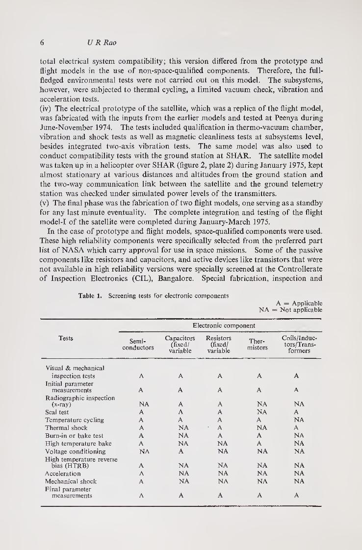
Table 1. Screening tests for electronic components A = Applicable
NA = Not applicable
Electronic component
Tests Semi¬ conductors
Capacitors (fixed/
variable
Resistors (fixed/
variable
Ther¬ mistors
Coils/Induc¬ tors/Trans¬
formers
Visual & mechanical inspection tests A A A A A
Initial parameter measurements A A A A A
Radiographic inspection (x-ray) NA A A NA NA
Seal test A A A NA A Temperature cycling A A A A NA
Thermal shock A NA ■ A NA A
Burn-in or bake test A NA A A NA
High temperature bake A NA NA A NA Voltage conditioning NA A NA NA NA
High temperature reverse bias (HTRB) A NA NA NA NA
Acceleration A NA NA NA NA Mechanical shock A NA NA NA NA Final parameter
measurements A A A A A

An overview of the Aryabhata project
a <D
X P <z>
o •3 o u
o (L>
73 u P O X p o u a a .0 'P a o s *0
<D Qh
p a> g p o u
*> P w
s
H a>
73 O
3
a3 in
£$ 41 o' o o o 7 >n fcl
O
2 3 2 g 8. 8. a I -3 s X >
3 O 111 >->
0 o <N
Tf O (N «-*
o 2 '5 3 ed m % H 00 3 2 Q £
2 05 £
O' 2 W M
• • oj <u o o a« _• U 5 3 o
< P Oh Z
i s—>
N
ffl N 2 0 1 X
0
»/o <N (N
co
6 0
f uo a
X P O
6 1
CO /—s
W 8
3) s—✓
3
10
O- a P
rate
So <D p
<d 73 O
So O O
d>
O p 0
+-> O
Z
Oh 3
£ g* & 2
W Hh
a a <
U U O o T—I T—I
-H + *0 vo >n t-h
■m 2 o o
u X <N
<D a
u X vo .g
P § .2 o -£ 73
aupfi
u y S-H -H 3 -H -H ^
5 <N
o o VO CO
T3 ■+-> rX o o
ffi O
o 73 11 3 P
<D O. >>
° 8 O >> Oh O
I ^ <D o v- u P P
O u - °H
-H-H o
a £ 3 ^ P <N Ih <u • • a
<D d>
X 60 £
a 3 P 00
2 o
£
< z
a> .ti o- a 2 8|S a < Q
U o T—I
-H
o
-H © o ^ o
H XI
2 3>
a §
ll _. %%
M u ft <2 « 2 .0 o
< Z
2)
E

8 U R Rao
approval procedures were evolved to ensure the overall reliability of the spacecraft.
These were strictly adhered to at both subsystem and system levels. The environ¬
mental specification for onboard electronic subsystems are listed in table 1. The
screening tests for electronic components are listed in table 2.
3.2 Ground segment and mission operation
3.2a Ground stations
The primary ground station for receiving data and commanding the satellite was
located at Sriharikota (SHAR) near Madras. The station consisted of a fully steer¬
able yagi antenna array (figure 2, plate 2) and a complete set-up for receiving the data
from the satellite, displaying them, and conducting preliminary analysis to quickly
determine the state of the health of the satellite. Besides, facilities to command the
satellite from the ground were established. In addition, a tracking network consisting
of a Doppler, interferometry and tone ranging system was also installed at SHAR,
to derive the orbital parameters of the satellite correct to 1° in elevation and azimuth
and ^ 500 m in range. The functioning of the entire ground station was also tested
using a helicopter-borne satellite model and simulating the transmitter power levels
for the maximum range that the satellite will have during its orbit, to ensure that the
ground station can receive the telemetered data from the satellite and send commands
to the satellite at any distance above 10° elevation.
The ground station at Moscow belonging to the USSR Academy of Sciences
received additional data from the satellite thus enhancing the total data coverage
from the satellite. A telecommand station built at the ISRO Satellite Centre,
Bangalore was also installed at Moscow for commanding the satellite from Moscow
to get both real time and stored data. To further increase the data coverage, the
French Space Agency, CNES, provided real-time telemetry reception and tracking
of the satellite in the initial phase. The optical Baker-Nunn camera at Nainital
observatory was also used for optical tracking of Aryabhata.
3.2b Mission operations
A Mission Operations and Control Centre was set up at Peenya, Bangalore, to co¬
ordinate the commanding as well as data-gathering programme from various ground
stations. From this Centre, the information regarding the radio-visibility of the
satellite for the ground stations was transmitted. Both the quick-look data which
provided information on the health of the satellite almost on real time basis as well as
comprehensive data were sent from each of the ground stations to the control centre
at Bangalore. The control centre performed the necessary analysis and decided on
the appropriate commands to be executed for the subsequent passes over the ground
stations. Detailed data processing and conditioning for further analysis were also
carried out at Bangalore and transmitted to various scientists.
3.3. Infrastructure
The work of setting up the necessary infrastructure for fabricating and testing various

An overview of the Aryabhata project 9
subsystems of the satellite was taken up immediately after the project was set up.
These facilities included highly sophisticated electronics laboratories, a clean room
for the final assembly of the satellite, thermal laboratories, control and stabilisation
laboratories, antenna testing facilities, a small workshop and a draughting section.
In addition to these general facilities, a few specialised facilities were also set up.
These included a dynamic balancing machine for balancing the fully integrated satel¬
lite, equipment for measuring the centre of gravity and moments of inertia of the
satellite, and a space simulation or thermo-vacuum chamber, capable of simulating
space environmental conditions such as temperature ranging from — 100°C to +100°C
at a pressure of 10“6 torr. This thermovacuum chamber was extensively used to test
and qualify the different satellite subsystems at various stages of the developmental
programme.
4. Pre-launch and launch aspects
After complete integration and testing at Bangalore, the fully integrated satellite
was transported to the USSR Cosmodrome in a specially qualified ‘ shock-proof ’
container. The satellite inside the container was isolated with helical springs to
dampen the mechanical shock and vibration and the container design was qualified
by actual measurements during transportation over typical roads to ensure that the
container was adequately safe to carry the satellite. At the Cosmodrome, the satellite
was disassembled into its three main parts — bottom shell, deck plate with instru¬
mentation and top shell (figure 3, plate 3). These were physically inspected and then
electrically tested with the entire check-out system. After this the satellite was
integrated once again, and a thorough check was conducted on the integrated
satellite, both prior to and after mating with the rocket carrier.
Results of all the tests and the state of readiness of the satellite as well as the rocket
were critically examined by a specially constituted launch commission, before fixing
the date and time of launch. The readiness of the ground stations at SHAR, Moscow
and Bangalore was checked, round the clock, through the dedicated communication
link specially set up for this purpose between the Cosmodrome, Moscow ground
station, SHAR ground station and the Mission Control Centre at Bangalore.
Aryabhata was successfully launched into a near-earth orbit at 1300 hr 1ST, on
19 April 1975. The orbital parameters immediately after the injection were apogee
height 620 km, perigee height 562 km, and inclination 50-7°.
5. Orbital performance
Aryabhata was controlled during the initial phase from the ground station at Bears
Lake, USSR, and during the normal phase from the SHAR ground station.
The satellite was powered immediately after its separation from the rocket, about
30 min after the launch, as could be seen from the telemetry signals received at SHAR
for the first time during orbit 2. However it was found that (i) the satellite was
tumbling at a rate of about 0-3° per second instead of spinning, and (ii) ±9 V was
not reaching the aeronomy experiment. All other subsystems, including power,
telecommand, telemetry, communication, attitude sensors, thermal control system

10 U R Rao
and the scientific experiments, were functioning normally. In spite of the fact that
the satellite was tumbling, the temperature of various subsystems was found to be
within the expected limits, thus proving the excellent performance of the thermal
control system.
Satisfactory signals were received from the satellite till orbit 17 after which some
problems like sudden drop in the signals and non-synchronisation of telemetry frames
were noticed. After carrying out some command operations to understand the
above problems, it was observed during orbit 41 that+9 V regulator output supplying
power to the three scientific experiments, was absent. All other power lines were work¬
ing normally. It was then decided to switch off the three scientific experiments
through ground command and make the satellite technologically functional. In
orbit 45, a spin command was sent from the ground and the satellite was spin-
stabilised at 50 rev/min.
After switching off the experiments, regular operation of the satellite was carried
out for the reception of real-time and play-back data. Analysis of both quick-look
and complete data was conducted to verify the performance of the onboard techno¬
logical subsystems. A brief summary of the performance of various subsystems
follows.
(i) The telemetry downlink functioned very well both in real-time and play-back
modes. The received ground signal strength on an average was always more
than —125 dBW which provided a good signal/noise ratio for interruption-
free data acquisition. The frequency stability of the onboard transmitter
was observed to be 0-00015 %. The observed bit error rates during both the
play-back and real-time mode were around 0-047% including the ground
station instrumentation errors.
(ii) Consistent and reliable operation of telecommand uplink was established
by successful execution of ground commands. The worst case onboard
signal strength was observed to be —86 dBM, which was consistent with
design specifications. The capability of execution of commands even at
very low elevations provided a greater operation manoeuvre period over each
pass. (iii) The state vector information (initial conditions) of one orbit per week
received from USSR was mainly used for generating target indications.
The range and range-rate data received from SHAR were found to be offset
by ±5 km and ±25 ms when compared to the best predictions. They were
quite accurate to do the necessary orbital analysis and updatings and also
gave confidence to generate target indication independently.
(iv) The performance of the thermal control system was quite satisfactory. All
the electronic subsystems were kept within the desired temperature limits.
The thermal control system performance characteristics for battery and
transmitter are given in figure 4. (v) Even though the actual theoretical estimates showed that the time constant
of the decay could be about 220 days based on the calculations of eddy
current losses in the conducting parts of the satellite, for the initial design
the value of about 22-4 days was used based on the actual observations on
‘ Cosmos’ satellites of roughly the same dimension as Aryabhata. Due to the
extreme care taken in using non-magnetic materials on the spacecraft, actual

An overview of the Aryabhata project 11
100 300 500 700 900 1100 1300 1500
Orbit number
0 200 400 600 800 1000 1200 1400
Orbit number
Figure 4. Inflight thermal control performance on Aryabhata
observations after the Aryabhata launch have shown that the decay constant
is quite large, of the order of 150 days which has been responsible for the
extension of the useful life-time of Aryabhata well beyond the original
estimate of 6 months.
In addition to the regular operations of the satellite, a number of technological
experiments were also carried out with a view to study the feasibility of using a
space platform for relaying different types of complex data for various practical
applications.
These technological experiments were essentially based on the use of the onboard
telecommand receiver and transmitter in the transponder mode for transmitting data
from one station to another through the satellite. In the first instance, a voice trans¬
mission experiment was performed wherein recorded speech was transmitted from
SHAR and received at Bangalore via Aryabhata. The quality of the voice reception
was very good. Subsequently, electrocardiogram (ECG) signals were similarly
transmitted from SHAR and received at Bangalore via Aryabhata. The results were
quite encouraging and demonstrated the feasibility of extending medical help to
remote areas through the use of satellites.
The third experiment involved the transmission of weather data like temperature,
wind speed, wind direction etc., from a standard data collection platform through the
satellite. The data collection platform was set up at Sriharikota through the assist¬
ance of the India Meteorological Department (IMD), Poona. The experiment was
conducted successfully and the results were found to be well within the limits of

12 U R Rao
accuracy required for meteorological purposes. The experience gained through this
experiment will be valuable for future programmes in designing operational satellites
for gathering meteorological data from remotely located data collection platforms.
6. Concluding remarks
This first Indian satellite is in many ways as sophisticated as many satellites which
are being flown by other countries. For example, the satellite employs more than
12,000 active and passive electronic components in addition to 20,000 solar cells
and other structural parts. There are more than 25,000 interconnections within the
satellite; the total length of all connecting wires exceeds 6 km. In fact, this is the
first satellite which has used, on a large scale, the low power Cosmos integrated
circuits.
Precisely what have we learnt from the first satellite and how is it going to be helpful
in our programme? We have achieved the technology of design and fabrication of a
completely space-worthy satellite which includes structural design, fabrication and
testing, thermal and power control systems, stabilisation and attitude sensor systems.
We have established our ability to transmit complicated data from the satellite to the
ground, receive and process the data on the ground, command the satellite from the
ground and perform essential functions on the satellite. A complete tracking net¬
work to enable us to track the exact position and velocity coordinates of the satellite
has been set up. We have developed competence in the fields of orbital predictions
and quality control. A firm base has thus been established with which it is now
possible to design and fabricate application technology satellites.
Encouraged by the success achieved through Aryabhata, an agreement to launch a
second satellite from USSR was signed two days after the successful launch of the
first. This will be an application technology satellite called SEO (Satellite for Earth
Observations) which is scheduled to be launched before the end of 1978. SEO has
been designed primarily to carry out earth observations of relevance to Indian needs,
and will have two TV cameras and three microwave radiometers. The TV cameras
will provide pictures over India, each picture covering an area of about 340 X 340 km
with a resolution of 1 km2. Photographs will be taken in two spectral bands, one in
the visible (0-54 to 0 66 microns) and the other in the near infrared (0-75 to 0-85
microns). The microwave radiometer system (SAMIR) consists of a two frequency
Dickie type radiometer operating at 19-35 GHz and 22-235 GHz. SAMIR will detect
the fluctuations of microwave radiations mainly from the sea surface; these fluctua¬
tions will carry the signature of the sea state and surface temperature. The detection
is in terms of a brightness temperature with a resolution typically of the order of 1°K.
The data from these primary payloads will enable studies in the area of earth resources
especially related to hydrology, forestry, oceanography and meteorology.
Besides, SEO plans to realise a set of secondary objectives that include the space
qualification of indigenously developed thermal paints, heat pipe and solar cells.
Studies in cosmic x-rays and conducting data collection platform experiments of
relevance to meteorology also form other secondary objectives of SEO. The remote
meteorological data collection will be carried out with about 10-12 platforms mainly
distributed over inaccessible regions. The satellite mainframe of SEO uses the results of the developmental efforts on

An overview of the Aryabhata project 13
Aryabhata to a considerable extent. These include utilisation of the same structural
design procedures, thermal control system, low bit rate telemetry system as well as
attitude control and sensing system. The primary difference is mainly in the payload
to carry out spin-axis control operations, which did not exist in Aryabhata. Planning
the SEO configuration in this fashion has enabled considerable saving in time and
in the overall cost of the project.
The successful launch and conduct of the proposed experiments with SEO will be
a major milestone in the realisation of ISRO’s goals with the primary emphasis on
the communication and remote sensing applications.
Acknowledgements
Prof. S Dhawan, Chairman, Indian Space Research Organisation was a great source
of inspiration to all the persons working on the Aryabhata project. His constant
guidance and help is gratefully acknowledged. The USSR Academy of Sciences
provided a number of subsystems and also considerable technical help beside the
launch assistance in the execution of the project. The Indian Space Research Orga¬
nisation is very grateful to the technical collaboration provided by the Soviet Union.
A number of public and private sector enterprises within the country have helped in
the execution of this project. It is with great pleasure that we wish to acknowledge
the valuable help provided by the Hindustan Aeronautics Limited, Controllerate
of Inspection Electronics, National Aeronautical Laboratory, Bharat Electronics
Limited, Hindustan Machine Tools Limited, Indian Institute of Science and Hegde &
Golay Limited, all at Bangalore, and Electronics Corporation of India Limited,
Hyderabad, Bhabha Atomic Research Centre, Bombay, Overseas Communication
Services, Aircraft & Systems Training Establishment and many other institutions all
over the country. Without their cooperation, this national project could not have
been completed in time. The timely help provided by the Karnataka Stare Govern¬
ment in giving the sheds and various other facilities at Peenya is also gratefully ack¬
nowledged.

.
'

An overview of the Aryabhata project 15
Plate 1
Figure 1. Photograph of Aryabhata

16 U R Rao
Plate 2
Figure 2. Photograph showing the configuration of the ground station at Sriharikota

An overview of the Aryabhata project 17
Plate 3
Figure 3. Photograph showing Aryabhata in the dis-assembled form

»
The stabilisation system
P S GOEL, P N SRINIVASAN and N K MALIK ISRO Satellite Centre, Peenya Bangalore 560 058
MS received 28 April 1977; revised 17 November 1977
Abstract. The attitude stabilisation of Aryabhata was accomplished by spinning it about its axis of maximum moment of inertia. The spin stabilisation ensures satisfactory thermal control, uniform power generation through the body mounted solar panels and the scan capability for the scientific payloads. To bring down the nutation of the spinning spacecraft to a value well within the specified limits, a fluid- in-tube damper was also provided.
The design philosophy, specifications, details and the dynamics of such a system are presented in this paper along with the qualification and performance evaluation tests of the components and subsystems. Also, the in-orbit performance of the stabi- sation system is discussed.
Keywords. Satellite stabilisation; attitude control; spin-stabilisation; spin-up system.
1. Introduction
It is well-known that the gyroscopic stiffness provided by spinning a spacecraft about
its axis of maximum moment of inertia gives sufficient stability to its attitude against
environmental forces arising from aerodynamic, magnetic and solar radiation effects.
In addition, spin stabilisation helps in proper thermal control and ensures uniform
power generation from the body-mounted solar panels. Further, it enables the
onboard scientific experiments to observe both in the pointed and scan modes along
and perpendicular to the spin axis respectively. With these considerations in mind,
it was decided to employ a simple spin-up mechanism using cold gas jets for stabilising
Aryabhata. As wide tolerances for the spin rate were accepted by the scientific
experiments, a simple blow-down mode was considered feasible. Further, a fluid-
in-tube type of nutation damper was employed to damp out the initial coning of
the satellite resulting from the disturbances during the separation of the satellite
from the rocket. As no specific pointing requirements were projected, attitude
orientation capability was not incorporated; however, slow drift in the spin axis
orientation was considered desirable for large space coverage.
2. Design philosophy
The higher limit on the spin rate was fixed at 90 rev/min based on telemetry and
attitude reconstruction considerations.
A list of symbols appears at the end of the paper.
19

20 P S Goel, P N Srinivasan and N K Malik
The spin decay which is mainly caused by the magnetic drag, has been calculated
for two cases.
(i) The best case assuming the thin structural shell as a sphere and the rest of the
conducting mass as a cylinder, for which the time constant of the spin rate
decay worked out to be about 276 days.
(ii) The worst case with entire conducting weight taken as a thin spherical shell
for which the time constant worked out to be 31.2 days. However, a similar
Soviet satellite, Inter-Cosmos 106, launched into a similar orbit, had a spin
decay time constant of only 22.3 days which was assumed for the worst case
estimate from gas storage considerations for the designed operational life of
6 months.
After injection into orbit, the satellite has to be spun from zero to 90 rev/min. For
subsequent spin-ups (from 15 to 90 rev/min), less gas energy is required compared
to the initial spin-up. To standardise the system and considering the size of the
available gas bottles, it was decided to have similar spin-up units. Further, it was
decided to utilise two units for the initial spin-up operation as gas bottles with storing
capacity of 1 kg were available. The spin rate increase is given by
(1) W= Ml IspIIzz.
For dry air 7sp=60 s; also /=0.95 m; A7=mass of the gas in each bottle=l kg.
The specifications of the stabilisation system were:
10-90 rev/min
less than 0.1°
less than 0.1°
less than 21°/s
spin rate
half cone angle
dynamic unbalance
transverse velocity at the separation
moment of inertia about spin axis, Izz
spin decay time constant
opeiational life of the satellite
98.5 kg m2 (flight-1 model)
22.3 days (worst case)
6 months.
3. Design details
3.1. Spin-up system
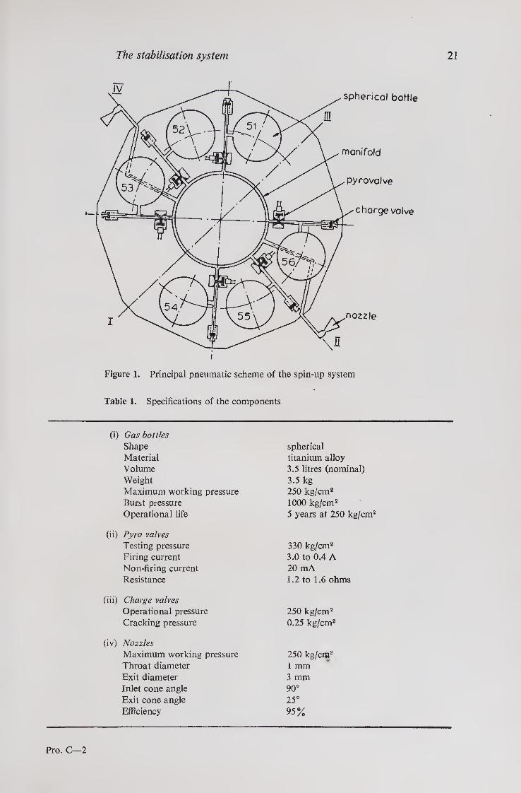
Figure 1 shows the schematic layout of the spin-up system. The six spin-up blocks,
each consisting of a gas bottle, a charge valve and a pyro valve, were connected to a
common manifold. The manifold was connected to a pair of nozzles, thus con¬
necting each spin-up block to the same nozzles. The specifications of the various
components are given in table 1. The various components were assembled through mechanical connections and
welded joints with a stainless steel pipe of 4 mm inner diameter and 6 mm outer
diameter.
The stabilisation system 21
spherical bottle
nozzle
Figure 1. Principal pneumatic scheme of the spin-up system
Table 1. Specifications of the components
(i) Gas bottles
Shape spherical Material titanium alloy Volume 3.5 litres (nominal) Weight 3.5 kg Maximum working pressure 250 kg/cm2 Burst pressure 1000 kg/cm2 Operational life 5 years at 250 lcg/crri
(ii) Pyro valves
Testing pressure 330 kg/cm2 Firing current 3.0 to 0.4 A Non-firing current 20 mA Resistance 1.2 to 1.6 ohms
(iii) Charge valves
Operational pressure 250 kg/cm2 Cracking pressure 0.25 kg/cm2
(iv) Nozzles
Maximum working pressure 250 kg/cm2 Throat diameter 1 mm Exit diameter 3 mm Inlet cone angle 90° Exit cone angle 25° Efficiency 95%
Pro. C—2

22 P S Goel, P N Srinivasan and N K Malik
3.2. Electrical circuits
The pyrocharges get ignited when a minimum current of 0.4 A is passed through for
at least 10 ms. For redundancy, each pyrovalve was fitted with two such pyro¬
charges, connected in parallel.
Figure 2 shows the electrical circuit used for firing the pyrovalves. Each pyro
valve, in series with a 9.1 ohm, 6.5 W resistor, was connected to the 22-28 V battery
supply through two normally open relays connected in parallel. A minimum of
1.5 A current was passed for 250 ms on command. A guard command, called
spin arm command, was provided to safeguard against spurious commands. The
spin commands are to be operated within 40 s of the spin arm command. The
complete status of the spin-up system was telemetered to the ground.
4. Analysis of spin dynamics
Considering the satellite as a rigid body, with body fixed principal moment of
inertia axes X, Y, Z, rotating with velocity Wx, Wy and Wz respectively, the equations
of motion are given by
lxx Wx + (7ZZ - Iyy) Wy Wz —Tx ; (2)
Iyy Wy + (Ixx - 7ZZ) Wx W2 = Ty- (3)
/„ W2 + {Iyy-U Wx Wy = TZ. (4)
In the absence of torques, the transverse velocity for rotationally symmetric body is
given as
Wx = Wr cos Q. t, (5)
Wy = WT sin Q. t, (6)
where Q = [Izz/(lxx Iyy)l/2~ 1] Wz and WT = initial transverse velocity.
Figure 2. Electrical circuit of the spin-up system

The stabilisation system 23
This transverse velocity results in coning of the spin axis about the total angular
momentum vector. The coning angle is given by
tan v=[(IxxI„y/*II„ Wz\ WT. (7)
In the absence of any internal dissipation in the body, the body would be stable
when spinning about its axis of maximum or minimum moment of inertia. But
the inherent internal dissipation in the body (i.e., structural, fuel sloshing or
any moving part in the satellite) makes the spinning about the axis of maximum
moment of inertia a criterion for stability.
In the blow-down mode, the thrust as a function of time is
F=CxAtP0 1 + (fc-1) IV
At (R0T0gk)1/‘‘ L2-V \k+ll
k+\ F7!
-2k/k-l
where Cx + * PJPX
Equations (2) to (4) are programmed on a computer taking into consideration the
various misalignment torques. The misalignment torques will result in additional
transverse velocity apart from separation disturbances. For the allowable limit of
10% increase in transverse velocity because of misalignments over the initial separa¬
tion velocity, the allowable tolerances were < 5 % in case of maximum differential
thrust for two nozzles and 1° for angular misalignment of the nozzles.
Since the dynamic unbalance had to be limited to 0T° in terms of principal axes,
the cross products of inertia had to be
4z, Lz < 0-0012 (/2Z — Ixx).
This was ensured by dynamically balancing the satellite using a vertical dynamic
balancing machine.
5. Nutation damper
Figure 3 shows a sketch of the fluid-in-tube nutation damper which was a
fibreglass toroidal hollow tube, partially filled with silicone oil. The damper was
fixed to the top structural plate through eight supporting lugs.
The silicone oil moves in the damper with constant angular velocity till the nutation
angle decays to a residual value. This results in the dissipation of the transverse
energy at a constant rate and hence the coning angle decays. The residual coning is
governed by frictional drag and acceleration torques due to coning. When these two
are equal, further dissipation takes place at a very slow rate, the flow being laminar.
The residual coning angle is given by (Rogers 1959)
V res t,n \ 4Rp a, sin n/2 )

24 P S Goel, P N Srinivasan and N K Malik
fibr< with
Figure 3. Nutation damper
For the nutation damper in Aryabhata, the residual coning angle of the satellite was
26 min. The time for the coning angle to decay from the initial value to the final
value vf was 1-2 min based on the formula
1 — cos Vj/cOS vf t = K/V4 wz(ilixx-ili2y
with Ws=90 rev/min and vt=l-2°.
6. Qualification
The system was subjected to various qualification and performance evaluation tests
at component and subsystem level for different models of the satellite as listed below.
(i) The vibration test was carried out on the spin-up system along all the three
axes and subsequently tested for leaks for various qualifying and develop¬
mental models. Six models were tested for leak in atmosphere and vacuum
using a helium leak detector to ensure leakproofness. One model was
stored in pressurized condition in vacuum for 6 months and then tested for
leak etc., to ensure stability in the vacuum condition.
(ii) The thrust impulse was determined for the five models in vacuum chambers.
(iii) The gas bottles were qualified to store gas for 5 years at 250 kg/cm2 pressure.
The temperature cycles from — 10°C to + 50°C were simulated and their
effect on leakage was studied.
(iv) Pyro valves were qualified to operate at temperatures ranging from — 50°C
to +50°C and pressures upto 300 kg/cm2; leakage was found to be less
than 1 x 10⁻⁵ Torr litre per second.

The stabilisation system 25
(v) The charge valves were qualified to have a nominal life of 6 months under
pressures of 250 kg/cm2, temperatures —40°C to -f50°C. The leak rate
was less than 1-75 X 10~3 istorr litres per second.
(vi) Totally 22 nozzles were tested in vacuum using a thrust measuring equipment
with 2% accuracy. Only the pairs of nozzles whose differential thrust was
less than 1 % were fitted in the system.
(vii) The nutation damper was qualified against vibration by testing for leak
before and after the vibration. The bonding of the stainless steel lugs with
fibreglass was also qualified for temperature cycling, vacuum and vibration
specifications.
(viii) The performance of the damper was evaluated on a 3-axis air bearing. The
coning decay time of 1.2 min and the residual coning angle of less than
0.1° was estimated from this data.
(ix) Independent electiical tests were conducted on the spin-up system for
checking the electrical connections, continuity, insulation resistance, etc.
An ‘ autonomous test console ’ was made to test the system and the
continuity of the pyro charges, ensuring non-firing of the charges during the
tests.
Figure 4. Spin build-up curve for Aryabhata

26 P S Goel, P N Srinivasan and N K Malik
(x) All these independent tests were conducted on all models of the satellite.
In addition, complex tests were conducted with prototype and flight
model to ensure proper interface with the telecommand parameters, tele¬
metry monitoring and sensor inputs. A special test was conducted to fire
the pyrovalves in the prototype model. The complex tests were repeated
at the USSR Cosmodrome.
(xi) The flight model of the spin-up system was tested for leaks at the Cosmo¬
drome and charged with dry air as per the requirements.
7. Performance in the orbit
Soon after launching, it was observed that the satellite did not spin as per the design
and the spin command was, therefore, given to fire gas bottle 2 in the 45th orbit.
The spacecraft attained the spin rate of 50.3 rev/min which was very close to the
predicted value. The spin build-up analysis (figure 4) showed that the first two
gas bottles did not get emptied and the simulation studies indicated that the mal¬
function of a relay in the pyrovalve circuit was a cause of the initial spin failure.
The actual spin decay was found to be much lower than that calculated for the
worst case and the spin decay time constant was found to be about 154 days
(figure 5).
It was extrapolated using sun sensor data that the residual coning angle attained a
value less than 0.05°.
8. Conclusions
The spin-up system has functioned satisfactorily with spin rate as calculated. The
spin decay has been found to be much slower than that observed for a similar Soviet
spacecraft Cosmos 106 and the estimated operational life of the satellite of 6 months
is thereby extended to beyond two years. The residual coning angle is very close
to the designed value of less than 0.1°.
Figure 5. Spin decay curve for Aryabhata
400 re spun
6 June 1976

The stabilisation system 27
Acknowledgement
The authors wish to thank Prof. U R Rao for his valuable guidance and encourage¬ ment.
List of symbols
A
At
at
cf g
sp
Ixxi lyy
k
l
M
n
Po
Pi
Ro r
RP
To
V
w e
v
P
wetted area of the tube (m2)
throat area (m2)
cross-sectional area of the tube (m2)
drag coefficient
gravitational constant (9.81 m/s2)
specific impulse of the gas (s)
moments of inertia about transverse axes (kg m2)
moment of inertia about spin axis (kg m2)
specific heat ratio for the gas
arm length (m)
mass of the gas (kg)
angle of fluid column filled
initial gas pressure (kg/m2)
inlet pressure at nozzles (kg/m2)
gas constant
radius of the damper tube (m)
mounting distance of tube plane
initial temperature (K)
volume of gas bottles (m3)
angular velocity (rad/s)
expansion ratio
coning angle
density of the fluid (kg/m3)
Reference
Rogers E E 1959 US Naval Ordinance Test Std. Rep. No. 10 P 565

■|1 ;i 'i? f I
’
.

The power system
S Y RAMAKRISHNAN, R S MATHUR, M SUBRAMANIAN,
T KANTHIMATHINATHAN, SUDARSHAN SARPANGAL,
S T VENKATARAMANAN and N S SAVALGI ISRO Satellite Centre, Peenya, Bangalore 560 058
MS received 28 April 1977; revised 20 December 1977
Abstract. The paper describes, in detail, the power system for Aryabhata. The various elements of the power system—solar array, storage battery and the power conditioners and control units—are covered. The in-orbit performance of the power system is dealt with, highlighting the probable reasons for the failure of one of the bus-lines of the power system.
Keywords. Solar array; array voltage limiter; power generation; storage; power conditioning and control; protective devices; grounding.
1. Introduction
The most widely used power source for a spacecraft is a panel of silicon solar cells
which convert incident solar energy into electrical energy through photovoltaic
action. Since an earth-orbiting spacecraft does not receive solar radiation all the
time, a part of the generated power is stored in an electrochemical storage device
which complements the function of photovoltaic generators during the shadow
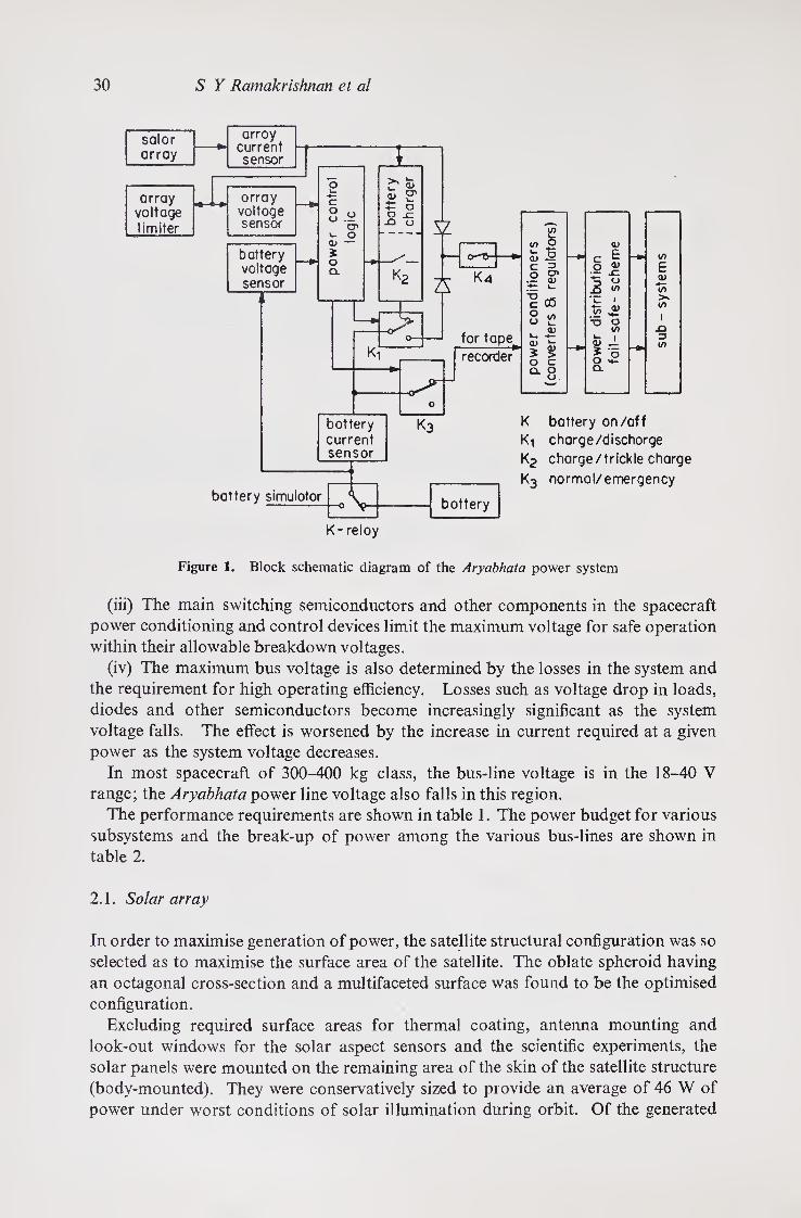
periods. The Aryabhata power system consisted of solar panels using n/p radiation
protected silicon cells, a Ni-Cd storage battery, a solar array voltage limiter, a power
control unit as a battery controller, power conditioning regulators, converters and
protective devices which are mainly as load interface units (figure 1).
2. Design philosophy and evolution
The power system for Aryabhata was designed to provide reliable and uninterrupted
power for various subsystems at the required voltage levels. The system design is
based on a highly reliable, single unit system rather than on redundant units, for
power dissipation and weight of a redundant system exceeds tolerable limits.
The useful range of operating voltages of the power source is decided as follows.
(i) The minimum operating voltage for the battery is determined by the maximum
bus line voltage required for the various subsystems.
(ii) The maximum operating voltage of the battery is limited by the number of cells
required to be connected in series which decreases reliability. Hence a trade-off
occurs between reliability of the system and the operating (max) voltage.
29
30 S Y Rarnakrishnan et al
K- relay
Figure 1. Block schematic diagram of the Aryabhata power system
(iii) The main switching semiconductors and other components in the spacecraft
power conditioning and control devices limit the maximum voltage for safe operation
within their allowable breakdown voltages.
(iv) The maximum bus voltage is also determined by the losses in the system and
the requirement for high operating efficiency. Losses such as voltage drop in loads,
diodes and other semiconductors become increasingly significant as the system
voltage falls. The effect is worsened by the increase in current required at a given
power as the system voltage decreases.
In most spacecraft of 300-400 kg class, the bus-line voltage is in the 18-40 V
range; the Aryabhata power line voltage also falls in this region.
The performance requirements are shown in table 1. The power budget for various
subsystems and the break-up of power among the various bus-lines are shown in
table 2.
2.1. Solar array
In order to maximise generation of power, the satellite structural configuration was so
selected as to maximise the surface area of the satellite. The oblate spheroid having
an octagonal cross-section and a multifaceted surface was found to be the optimised
configuration.
Excluding required surface areas for thermal coating, antenna mounting and
look-out windows for the solar aspect sensors and the scientific experiments, the
solar panels were mounted on the remaining area of the skin of the satellite structure
(body-mounted). They were conservatively sized to provide an average of 46 W of
power under worst conditions of solar illumination during orbit. Of the generated

The power system 31
Table 1. Performance requirements of Aryabhata power system
1. Total surface area Area occupied by solar array View window f or experiments etc. Coated area
2. Array details
Total array surface
Packing efficiency Projection efficiency Power output Array voltage Array temperature Weight of the solar array Vibration level for the array Shock level for the array No. of shocks
3. Panel details
No. of panel types Shape of the panels No. of cut-outs Size of cut-outs
Type of mounting Mounting substrate No. of series cells/module No. of parallel cells/module
4. Cell details
Solar cell type Material Resistivity Efficiency Size
Anti-reflection coating Cover-glass thickness Spectral response
5. Ni-Cd battery
No. of cells Capacity of each cell Type of interconnection Operating temperature Operating voltage range Charge current Trickle charge current Efficiency of battery Size Weight Sealing
62,265 cm2 36,800 cm2 1380 cm2
24,285 cm2
36,800 cm2 distributed over the 26 facets to give practically uniform output
80% 20% (min) 46 W (average) 31.5 V (min) -70° to +125°C 31.5 kg 10 g at 80-1500 Hz for 10 min 20 g for a duration of 5-10 ms 20
7 square, trapezium and octagon 13 110x50 (8 Nos.), 135x150 (3 Nos.) 135x225 (1 No.) and 100x50
(1 No.) (all in mm) shingle fibreglass net 106 7 to 12
n/p silicon 10 ohm cm 9% at AMO 10x10; 10x12; 10x15;
10 x 18 and 10 x 20 mm SiO 0.5 mm 0.4 to 1.1 ^.m
20 10 AH series 0° to 40°C 22-28 V 700 mA 100 mA 80% 380 x 310 x 80 mm 16 kg hermetic

32 S Y Ramakrishnan et al
Table 1. Performance requirements of Aryabhata power system (contd.)
6. Power control unit
Charge mode Vs > Vb Trickle charge mode Vs> Vb Discharge mode Vs< Vb Emergency mode Vs< Vb
NB: In the emergency mode power is discharge relay stays ‘ sun-only ’ mode.
22V< Vb<27.8 V VB = 27.8±0.2 V 22V<Kb<27.8 V VB = 22.0±0.2 V cut-off to all the subsystems. Charge
at charge mode. All the subsystems operate in the
7. Current sensors
Output range 0 to 5 V Conversion factor 2V corresponds to 1 amp Sensing element and value Printed pattern 50 m ohms Output impedance 500 ohms (max) NB: In the case of battery current sensor where the current through the element
is bidirectional an off-set of 2.0 V is deliberately introduced. An output less than 2.0 V represents charge current.
8. Power conditioners
Bus voltage Regulation (line & load) Efficiency Ripple and spike Output impedance
Line ‘ on ’ transient Line ‘ off ’ transient Load ‘ on ’ transient Temperature coefficient
±14, —14, ±9 and —9 V 1 °/o
Between 80 and 85 % Less than 30 mV 250 m ohms for range 0 to 2 kHz 350 m ohms for range 2 to 100 kHz 1.5 ms 20 ms 400 ms Less than 80 ppm for range —15° ±55°C
9. Standby power drain in different units
Power control unit Voltage limiter Failsafe unit (each)
10. Test specifications
Temperature Vacuum Period
Vibration
Shock
No. of shocks
750 mW 300 mW 20 mW
-10° to ±50°C 10-6 torr 24 hr at each temperature extreme after stabilisation 1.5 to 4.5g at 10Hz 4.5 to 9.0g at 30-800 Hz 9.0 to 15.0g at 80-1500 Hz 15.0g at 1500-2500 Hz
20g for a duration of 5-10 ms
20
Along all the three mutu¬ ally perpen¬ dicular di¬ rections
power of 46 W (average), the battery was provided with a nominal 23 W. This can
be derived from the formula:
p = -*• CQ 1 +
Vs (1)
where PstL=solar array power; TL--load power; ^r=losses in power system subunits
expressed in terms of efficiency; fe=maximum eclipse duration in orbit; ^^ illumi¬
nated period in orbit corresponding to te; Vs=Vt Vc where rjb watt-hour efficiency
of the battery, «c=efficiency of the battery charger.

The power system, 33
The solar array was made of n/p, radiation protected solar cells arranged into
modules. Shingle-type mounting to increase packing efficiency was preferred to
flat-type mounting. The modules were bonded to a fibreglass net using an
epoxy adhesive. The cells had SiO coating to minimise reflection and cover slides
for piotection against charged particle radiation and micrometeoroid bombardment.
Isolation diodes were used to prevent the illuminated panels from being loaded by the
shadowed ones. The diodes were connected in series-parallel combination to
nullify the effects of malfunctioning diodes. The modules were made of series-
parallel combinations of cells to achieve desired voltage and current levels.
The minimum operating voltage of the array bus line was determined by the fol-
owing considerations.
A change in the illumination level does not markedly affect the array voltage.
As a secondary effect, the array open circuit voltage proportionately increases by 3 %
Table 2. Power budget
No. of units
Total power Operating Subsystem consumption time (min/ Remarks
(W) day)
Telemetry encoder 2 0.945 1440 Hot redundancy Telecommand receiver 2 1.196 1440 do Telecommand decoder 2 0.047 1440 do Telemetry transmitter 2 3.200 1440 Cold redundancy Sensor 1 0.482 1440 No redundancy Tone range unit 1 0.010 1440 No redundancy Scientific experiments 1 5.422 1440 No redundancy
Both ‘ OFF ‘ Tape recorder 1 3.64 120 min (Record) (Record) normally 5.74 12 min One at a (playback) (playback) time while
operating
Figure 2. Exploded view of the solar panels of Aryabhata

34 5 Y Ramakrishnctn et al
Figure 3. Computed characteristics of the solar array for various aspect angles and temperatures
in response to 100% increase in illumination. On the other hand, the cell open circuit
voltage falls approximately 2 4 mV/°C. In view of this ambiguity and variation in the
temperature equilibrium, it is desirable to keep the operating voltage lower than the
voltage corresponding to maximum power. Though the operating power is lower
than the maximum power by roughly 5%, this arrangement ensures uninter¬
rupted operation at the highest anticipated temperature under all operating
conditions.
Since the optimal voltage of the cell at the operating point was roughly 297 mV
corresponding to maximum anticipated temperature, 106 cells were connected in a
series string to obtain 31-5 V at the output of the array. Once the number of series
cells was determined, the parallel connections were subsequently worked out. In
the case of Aryabhata, since the panel shape and size were predetermined, the entire
area was optimally used by judiciously selecting cells from the available
sizes.
An exploded view of the solar panels mounted on the satellite is shown in figure 2.
The solar array mounted on the spacecraft had a projection efficiency ranging from
20% to 22%. This enabled the total surface area projected in space to receive the
solar illumination. The computed characteristics of the solar array for various
aspect angles and temperatures are shown in figure 3. It can be seen from this figure
that for different array temperatures ranging from —40°C to 127°C, the array short-
circuit current /sc varies between 1650 mA to a maximum of 2460 mA corresponding
to the change in the open-circuit voltage Voc from 41 V to 72 V. Consequently, the
maximum power generated varies between 42 W and 80 W. Generated power
depends both on the array temperature and on the aspect angle which determines
the illuminated surface area.

The power system 35
2.2. Storage battery
Rechargeable secondary batteries used in spacecraft of near-earth orbits of a high
shadow/sunlit ratio (0-475 for Aryabhata) must endure a long cycle life (3000 cycles
for Aryabhata) at comparatively large depths of discharge and should possess high
charge/discharge efficiencies. They must be operationally reliable. They are
requiied, in a few cases, to meet the launch phase power requirements. Spacecraft
batteries are also required to absorb or deliver large current transients, with moderate
changes in voltage for a few seconds. In addition, batteries must meet severe mecha¬
nical launch requirements and must be able to endure the space environment.
Apart from meeting the peak power demand, the battery is also required to accept
considerable amount of overcharge. During its life-time the satellite would be in
continuous sunlight for a few times during which the daily average solar array power
would exceed the average power used during other passes. In the case of Aryabhata
the anticipated period for 100% illumination was 11 days (nearly 165 orbits). In
such cases, the battery would receive overcharge current for a substantial fraction
of its life. Based on the requirements detailed above, Ni-Cd battery was chosen
as the suitable candidate for this application.
During the charging process, the evolution of oxygen from the positive plates
starts before oxidation is complete and increases rapidly when the top of charge
condition is reached. Charge acceptance from the negative plate is, however, more
efficient and hydrogen is not evolved until this electrode is practically fully charged.
With an excess of capacity provided at the negative electrode of the cell, no hydrogen
will be evolved during normal overcharge and the oxygen which does form will re¬
combine at moderate pressures so that the cell can be sealed. The negative electrodes
of the cells used in Aryabhata have a capacity 1-3 to 1-6 times greater than the positive
electrodes. Individual cells in the battery were hermetically sealed; this was supple¬
mented by further sealing the battery in order to increase the reliability of operation
under vacuum condition. The main advantages of sealed cells are that they do not
require maintenance, the electrolyte need not be removed or replenished and the
cells can be used in any position; all these stipulations must be fulfilled for spacecraft applications.
The mechanical and thermal design of the batteries are of great importance. Use
of flat, rectangular shapes, rather than cylindrical cells results in decreased volume
of the battery pack. Rectangular shape also helps effective thermal control, since
the heat generated due to discharge/overcharge of the battery is conducted to the
external surface of the spacecraft and then radiated. The battery was housed at
the centre of the deck plate where expected temperature fluctuations were minimal.
The positioning of this high density package also helped to improve mass properties.
The battery capacity was determined according to the formula
required capacity = Pt jEd • h(DOD), (2)
where P—system power, t=maximum discharge time (in hours); £d=average
discharge voltage of cells; «=number of series-connected cells; DOD=depth of
discharge. Substituting the various values and allowing a safety margin of 50%, a 10
Ahr battery was selected for the application.

36 S Y Ramakrishnan et al
The number of series connected cells was reduced to an optimum figure on reliabi¬
lity considerations. The reliability of the series-connected cells is strongly dependent
upon the cell with the shortest life. A short circuit of a cell will increase the current
density and accelerate the deterioration of the other cells in the series circuit. All the
cells picked out from the same production batch, were matched at an initial capacity
spread of 5%; but this spread was likely to increase during operation because of
difference in capacity or temperature between cells.
The positive and negative terminals were provided on two different connectors
with sufficient redundancy on the pins used. This apart, the individual cells were
available on a third connector for tests during flight qualification stages. The battery
was fully discharged after final testing using this connector and a full capacity charge
was given before the satellite was mated with the rocket carrier.
2.3. Current sensors
The currents delivered by solar array and battery were measured in order to evaluate
the performance of these power sources in-orbit. In the case of battery the charge
current was also measured. These parameters along with the array and battery
voltages indicated the power at any instant. The measurement was done by slipping
50 mil printed circuit resistors in the current paths and processing the voltage drop
across the resistors.
In the case of the battery, since the current through the 50 milliohms resistor was
bidirectional, an offset was introduced in order to increase the output level above zero
potential corresponding to zero current; in this case the charge current was desig¬
nated as negative. The output was compatible with the telemetry system with the
voltage in the range of 0-5V and impedance equal to 500 ohms.
2.4. Voltage limiter
The array power exceeds the average specified value when the cold solar panel emerges
from the shadow zone of the orbit. This places a step voltage increase on the solar
bus-line. The array voltage limiter introduced an additional load on solar array in
such cases, thus limiting it to a predetermined maximum so that components in the
power system subunits were protected against excessive array voltage.
The limiter was directly connected across the array. The circuit consisted of a
reference source, comparator, gate and driver. The array voltage was compared
against the reference value and additional load introduced appropriately. The limiter
consisted of three similar sections and one or more loads were operated depending on
the array excess power. The limiter would recover once the voltage came down to
the normal value. The power dissipating resistors were sufficiently derated and
mounted on a special heat-sinking plate in the package.
2.5. Power conditioners
The power output from the solar array or battery was conditioned to supply the
various subsystems at four standard bus voltages, all regulated within 1 %. The
positive bus voltages were supplied directly through high efficiency switching regu¬
lators whereas negative voltages were generated using d.c./a.c. converters followed

The power system 37
by switching regulators. The regulators were all protected internally against overload
and short circuit.
The choice of a switching type of regulator is based primarily on two con¬
siderations.
1. Efficiency of a switching regulator is very high and consequently power losses
are minimum. This, in turn, reduces the heat-sinking problems of power transistors.
2. The input-output differential can be very low compared to the series-type of
regulators.
The regulators work under the principle of power dumping. The energy from the
solar array is stored in the magnetic field of an inductor during the first half of the
switching cycle of a series switch and smoothly transferred to the output side during
the later half cycle, after filtering. Additional filtering is also used in order to reduce
the ripple to an acceptable limit.
The d.c./a.c. converters used for the negative regulators were of the conventional
grounded-emitter type followed by bridge-rectifiers and filters. They provided
floating level outputs and the positive was grounded at the regulator end to provide a
negative output voltage.
Despite the low power dissipation in all the series transistor switches and the high
derating allowed, all the transistors were mounted on the body of the regulator-
package using beryllium-oxide isolation washers which are thermally conductive.
Moreover, the transistors were protected against any accidental short to the ground
by using an epoxy adhesive which is an electrical insulator and thermal conductor.
2.6. Battery charger
The generated power at the solar array was partly stored in the Ni-Cd battery through
a high efficiency switching type of constant current charger. The principle is similar
to that explained for the regulators. In this case the battery forms the reference
source and the voltage across a fixed resistor in the current path is maintained constant
by comparing it in a closed-loop with the reference. In order to protect the battery
from damage due to excessive charge and to compensate for any internal losses, the
charging current is reduced once the battery reaches full charge condition. This is
termed as the trickle-charge current.
2.7. Power control unit
The power control unit performs the following functions.
(a) Smooth switchover of power source to the satellite from solar array to battery
and vice versa depending on the shadow/sunlit portions of the orbit.
(b) Switchover between charge/trickle charge modes depending on the battery
charge condition.
(c) Switch-off power to all the subsystems when the battery has considerably dis¬
charged, in order to protect it from permanent damage from excessive discharge;
the satellite will, however, work in the ‘ sun-only ’ mode. This situation is called
‘ emergency mode ’ of operation of the satellite.
The solar array and battery voltages were compared against a temperature-com¬
pensated stable reference and the various control relays Kv K2 and Ks (see figure 1)
were operated appropriately as per the logic conditions detailed in table 1. In the
Pro. C— 3

38 5 Y Ramakrishnan et al
case of the battery, its voltage changes due to internal impedance when the current
changes from the charge current of 700 mA, to the trickle charge current of 100 mA.
This provides some ambiguity in the sensing circuit and results in the chattering of the
relays. In order to avoid this, a small amount of hysteresis was introduced in the
control circuit.
2.8. Failsafe unit
Since separate regulators for each subsystem increase the total weight of the power
system and reduces its efficiency, few of the subsystems were provided with separate
regulators. In the former case protective devices were used to isolate the malfunc¬
tioning subsystems from the main line. The malfunction may be in the form of an
overload or short circuit.
The failsafe was interposed between the regulators and the various subsystems.
The failsafe cuts the power supply to the malfunctioning subsystem and effectively
arrests the propagation of malfunction. All subsystems operating with the redundant
units used separate failsafe both for the main and redundant ones.
The circuit is shown in figure 4a. Initially, when power is switched ‘on ’ Rx—R2
provide a small base current path for Qv The conducting transistor Qv in turn,
provides base current for Q2. Transistor Q2 now provides additional base current
path for Qv By cumulative action, both Qx and Qt fully reach the conditions of
saturation and operate as switches. The circuit has foldback characteristics as shown
in figuie 4b. The knee point is decided by resistor R3. In the case of a load in excess
of the knee point, transistor Qx will pull out of saturation due to inadequate base-
drive. This, in turn, pulls Q2 also out of saturation and as a result of degenerative
action both the transistors go off. The subsystem is now completely isolated
from the regulator and the other subsystems.
2.9. Grounding and special provisions
Interference between the various subsystems through the ground line was minimised
by using a single-point grounding scheme. The return paths of all the subsystems
were terminated at a single point as also the zero-potential points at all the regulators.
This point was eventually connected to the deck-plate of the satellite. Besides, power
Figure 4. Circuit diagrams for (a) positive failsafe and (b) negative failsafe

The power system 39
lines for all subsystems used shielded, twisted pairs of wires for minimising pick-ups
and magnetic field contribution due to circulating currents.
To facilitate the disconnection of the onboard battery from the spacecraft loads
during the periods between tests on ground, a relay switch (A-relay) as shown in
figure 1 was introduced in the battery line. The relay had a change-over switch for
selecting between the battery and the battery simulator during ground test. The
switch was closed prior to the launching and was kept closed throughout the life of
the spacecraft. Provision was also made to charge the battery during ground tests
when the satellite was powered by the battery simulator. In order to keep all the
subsystems ‘ off ’ during the launch phase, switch K\ was introduced in the main
power line. This switch was closed by a signal from the rocket carrier 22 min after
take-off. An alternate provision was also made to close the switch using the
separation signal in case of failure in the rocket signal. The switch remained closed
thereafter during the life of the spacecraft.
3. Performance evaluation and environmental tests
The power system in Aryabhata was required to give satisfactory performance as
detailed in table 1. This included the environment in the orbital conditions (tempe¬
rature and vacuum) and the severity of launch conditions (vibration and shock).
In order to evaluate the performance of the various subunits, special test equipment
were developed and fabricated in-house. These included a test console which in¬
corporated the solar array simulator and load simulators and a charge/discharge
unit. The array simulator provided the power for the satellite operation and had
characteristics similar to the array. The simulator characteristics could be adjusted
to any computed characteristic shown in figure 3. The battery charge/discharge unit
had a provision to charge and discharge the battery at the rate of 1 A. It had also
provision to discharge the individual cells after the battery reached 22 V, corres¬
ponding to emergency condition.
All the power system packages were tested under simulated environmental condi¬
tions in a thermovac chamber. Each prototype package was tested at — 15°C for
24 hr after stabilisation. The flight packages were tested at — 10°C and +50°C as
detailed above. Since the anticipated temperature maximum was -}-70°C at the
place where the isolation diode boxes were mounted, these boxes were tested for this
condition and qualified. The prototype battery was tested in the thermovac chamber
for the specified test conditions and its performance was found satisfactory. All the
packages were subjected to vibration and shock as per the specifications and
qualified.
Since the power control unit and the i 14 V regulators for the tape recorder were
directly connected to the battery, they were powered during launch as against other
regulators and subsystems which were ‘ off’. These units were tested for this condi¬
tion by powering them while being vibrated. The results did not show any deteriora¬
tion in their performance.
During the vibration test on the mechanical prototype model of the satellite, few
cells at the top octagonal panel were displaced. This was found to be due to high
transmissibility and the consequent excessive vibration level at the place where the
40 S Y Ramakrishnan et al
panel was mounted. This was corrected by redesigning and introducing stilfeners at appropriate places in the satellite structure.
The prototype and flight model solar arrays were tested under terrestrial sunlight condition at noon and the results were extrapolated by applying suitable corrections for atmospheric absorption etc., according to the formula
hc=(hc i+-4c a • • • • 4“/sc ae) XO-835 X 1350/iiX 0'22, (3)
where /sc=short circuit current in the composite structure of the solar array in the orbital conditions for the mean distance of the earth from the sun ; /sc 1... ■ /sc 26 ^measured value of the short circuit current of each panel under terrestrial conditions; 0-835=coefificient taking into account the difference in the sun’s radi¬ ation spectra at the outer atmosphere and on the surface of the earth; 1350 watts/m2 =the solar constant at the orbital height; E watts/m2=the solar intensity on the surface of the earth as measured by the pyroheliometer; 0 22—nominal projection efficiency of the solar panels mounted on the satellite body.
4. In-orbit performance
Telemetry data of power system parameters collected at SHAR (India) and at Bears Lake (USSR) indicated, in general, a satisfactory performance of the system in orbit. However, the -f-9V regulator line feeding the experiments was found to be absent after a few days of operation.
The solar array and battery supplied the needed energy for the operation of the spacecraft subsystems. The battery charger provided the specified charge and trickle charge currents. The power control unit operated as per the specifications (a) to switch the charger between the two modes of operation and (b) to switch the battery between charge and discharge modes.
Due to the satisfactory power position, the contingency provision made to switch ‘ off’ power in the case of an emergency has not been operated todate. The power conditioners provided regulated voltages at required currents quite satisfactorily and continue to do so.
5. Conclusions
The entire Aryabhata power system with the design philosophy, evolution and a detailed description of the various elements used in the system have been described in this paper. The environmental tests conducted on the system packages along with the performance evaluation of the system under the simulated environment have also been dealt with. The in-orbit performance of the system with reference to the failure in one of the regulator lines is reported.
To analyse the causes for the failure of the -f-9V regulator foi experiments, extensive simulation studies including simulation of environments were made on the proto¬ type satellite. Based on the results of this study it was concluded that the most likely cause would be the failure of one of the components rendering the regulator out-of-use for the rest of the mission period.
Performance evaluation of the power system has shown that it can work satis¬ factorily in the stringent space environment.

The thermal control system
H N MURTHY, V K KAILA, V PRASAD, D R BHANDARI, H BHOJARAJ and P P GUPTA Thermal Section, Mechanical Systems Division, ISRO Satellite Centre, Peenya, Bangalore 560 058
MS received 16 April 1977; revised 29 October 1977
Abstract. This paper presents the design, analysis and performance of the thermal control system of Aryabhata.
A passive thermal control system, using flat absorber-AK-512 black paint for the outer surface of the satellite and a combination of solar reflector-AK-512 white paint and mechanical polishing for the inner surfaces, was employed to maintain the tem¬ perature of all the electronics subsystems onboard the satellite within the specified limits of 0°C and 40°C during the operational life of the satellite.
The in-flight temperature data obtained from sixteen temperature sensors onboard the satellite was compared with the theoretically predicted temperature values and the agreement was good for all electronic subsystems housed within the framework of the satellite.
The observed deviations in temperature for the tape recorder, proportional counter package and gas bottles of the spin-up system are attributed to the assumptions made for the mathematical model. It has been found that by improving these approxima¬ tions, the deviations could be reduced to negligible values.
Keywords. Satellite thermal control; design; flight performance.
1. Introduction
The thermal control system of a satellite is expected to maintain the temperature of all the subsystems of a satellite within specified limits. Most of the subsystems in the satellite give their optimum performance in a specified temperature range. If the temperature limits are not restricted, deterioration in the performance, perma¬ nent damage or malfunction of a subsystem may result.
A thermal control system is designed considering all the sources of heat inputs to the satellite, i.e., sun, earth and internal heat generation, and by applying heat balance method to all surfaces of the satellite. Depending on the temperature limits of sub¬ systems and orbit parameters, a choice has to be made between passive and active thermal control systems.
It is generally possible to realise temperature control for a low power, near-earth satellite using a passive thermal control system. Moreover, a passive method for temperature control is preferred for its inherent reliability and low weight as com¬ pared to an active thermal control system.
Hence, before the selection of the thermal control system and its detailed design, data on the proposed orbit, structure of the satellite, power dissipation and its fluctua¬ tion have to be known. Relevant data for Aryabhata's thermal control system design were 600 km near-circular orbit with 51° inclination to the equatorial plane, and
A list of symbols appears at the end of the paper.
41
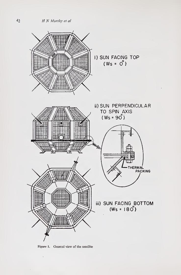
42 H N Murthy et al
i) SUN FACING TOP
(Ws = 0°)
ii) SUN PERPENDICULAR TO SPIN AXIS
(Ws* 90°)
THERMAL PACKING
iii) SUN FACING BOTTOM
(Ws = 180°)
Figure 1. General view of the satellite

The thermal control system
Table 1. Specified temperature ranges of various subsystems of Aryabhata
43
Subsystem Temperature range in °C
Tape recorder (TR-11) 0 to 40
Chemical battery 0 to 40
Transmitter -3 to 40
X-ray experiment box (proportional counter), Ex-12 — 15 to 55
All other subsystem boxes housed in the framework -1 to 40
Gas bottles -30 to 50
Charge valves -30 to 75
Pyrovalves -20 to 65
quasi-spherical polyhedron of 26 facets. The shape of the satellite, which has a weight of 358 kg, is shown in figure 1. The satellite is spin-stabilised about its axis of symmetry. The onboard power dissipation fluctuates between 23 W and 46 W depending on the functional requirements of the subsystems.
The temperature ranges within which the subsystems were to be maintained by using the thermal control system are given in table 1.
A survey showed that a great deal of literature was available on the design, development and testing aspects of a thermal control system. Basic principles are found in Kreith (1962), and discussions of thermal system design are found in many reports and journals (Semple 1968; Oshima and Oshima 1968; Fontana 1967, Finch et al 1968). Depending upon the type of facility available either solar simulation (Bernier et al 1965) or infra-red simulation (Hellmann 1970) could be adopted. If the facility could not accommodate the full size model then a scale model could be fabricated and tested (Miller and Wiebelt 1967).
The passive thermal control system for Aryabhata was to be designed on similar lines using the given data and to be analysed. The finalised system was to be achieved on the satellite structure and to be verified by conducting an infra-red simulation test.
2. Thermal design and related mathematical model
The design of a thermal control system is essentially an interactive process. It con¬ sists of selecting a combination of optical coefficients (as, the solar absorptance and <r, the infra-red emittance) of the various surfaces of the satellite and controlling the con¬ duction heat transfer between various parts of the satellite. The design process starts with the assumption of initial values for the optical-coefficients of the satellite for surfaces, and calculating the temperature distribution within the satellite for extreme cases, using these values. If the calculated temperatures for some of the subsystems are not within the specified range the controlling parameters are modified and the temperatures are recalculated using modified values. The process is repeated till a satisfactory design is arrived at.

44 H N Murthy et aI
2.1. Mathematical model
For temperature calculations of the satellite the ‘isothermal node method’ was used. The satellite was divided into a number of nodes so that the temperature variation within each node was small enough for the node to be considered as an isothermal unit. The heat balance equation for such a case can be written as
rate of change of enthalpy=solar radiation load-j-albedo load-j-earthshine load-f- internal heat dissipation+gain through conduction from other nodes+gain through radiation from other nodes —loss through radiation into space.
Mathematically, this can be represented as
WfdTfdt) = qsasArSi + + qe*eAFel + Pi
+ Y'i=i c«(J'J-r,)+ -<,.^,7,* (l)
where i — \, 2, ... n and j — 1, 2, 3, ... n.
The above set of equations were solved using the fouth-order Runge-Kutta method. Methods of calculating the various parameters on the right hand side of (1) are briefly presented below.
2.2. Calculation of solar load
Incident solar radiation on /th node is qs Arst when the satellite is in sunlit region of the orbit, and 0 when the satellite is in the shadow of the earth. (2)
In the case of a spin-stabilised satellite, the projected area in a given direction varies during each revolution of the satellite about its axis. The average projected area in any direction, assuming that it is not shadowed by any part of the satellite, is given by
AFs = A/n [ cos y cos j8 (£) + sin y sin /? sin £],
where £ = cos_18, if — 1 < 8 < 1,
= 77, if 8 < —1,
= 0, if 8 > 1,
and 8 = —cot f2 . cot y.
Figure 2a gives the axis system and the angles between the surface and the sun vector.
Values of AFx will obviously be zero for all internal nodes of the satellite. The mean solar constant is found to be 0-14 W/cm2 over the projected area near
the surface of the earth. The solar constant fluctuates by about 3-i % around its mean
value.

The thermal control system 45
Figure 2. Axis system and angles used for sun, albedo and earthshine load calcula¬ tions
2.3. Calculation of albedo and earthshine load
For estimating albedo radiation i.e., the solar radiation reflected by the earth, it is assumed that the solar radiation is diffusely reflected by the earth. The reflection factor varies depending upon the terrain and the weather conditions. An average value of reflectance of 0-35 is generally used and is found to give satisfactory results. The albedo load received by the /th node of the satellite is
i s, ' '
qsR dpop (3)
where A&t = AJ2 J^=Q Sx S2 S3 S, df d<f>,
and = cosine of the angle between local normal to an element of the earth surface and the sun direction,
52 =■* times the ratio of the average projected area in the direction of satellite-earth-element line to the total area of a node,
53 — cosine of the angle between local normal to the earth-element and the earth-element-satellite line.

46 H N Murthy et al
S^dtfjdcf) — the solid angle subtended by the earth element at the centre of gravity of the satellite,
At — area of the zth node.
For calculating the intensity of the earthshine load, the earth is approximated to a sphere radiating at a constant temperature. From the heat balance equation of the earth, the intensity of the earthshine can be written as
qe=qs{\-R)lA.
The earthshine load on j'th node is
qs(l-R)etAFetl4, (4)
where AFr, = 1 j2’=0 S2 S, d* d*,
and S2, S3 and are as defined in the case of albedo load. The co-ordinate system and the angles used in deriving (3) and (4) are shown in figures 2b and 2c.
2.4. Internal heat dissipation
Internal heat dissipation is the energy dissipated inside the satellite by the electronic components or heat generation in any of the moving parts of a mechanical system. This term varies with time due to power availability and the sequence of operation of the systems. In the case of Aryabhata, the maximum power consumed over a day is 46 W and the minimum power consumed averaged over a day is 23 W.
2.5. Radiation exchange factors
The radiation exchange factor or absorption factor is a complex function of the shape factors and the emittance values of the surfaces. An exact determination of this parameter can be made only after considering the multiple reflections within an en¬ closure. However, in the case of high emittance values and diffuse reflection, the following approximate equation gives a sufficiently accurate estimate.
fij — fi €j Fij/tO—Pi Fit) (1 ~pj Fjj) — pt pj FtJ FJt], (5)
where et and ej are the emittance and pt and pj are the reflectances of nodes / and j respectively. Also Fit, Fjj are the view factors of node i with node i and node j with node /' respectively and FJt is the view factor of node i with respect to node /.
2.6. Conduction exchange factors
The conduction exchange factor is calculated as the inverse of the total thermal resist¬ ance in the path of heat flow between the surfaces. Assuming one-dimensional con¬ duction, the equation for calculating the conduction factor is
1 ICu = i fcu + i iCjj'+1/a*X (6)

The thermal control system 47
where Cn and Cjj are conductances of node i and node j respectively and
aJt = ag + ar + ac-
where ag and ar are negligible as compared to ac. The value of ac is dependent upon surface finish, flatness of contact surface, materials surface and the pressure at the contacts. The value of ak varies between 0 02 and 2 W/cma °C. The expression suggested for calculating ac in case of rivetted lap joints is
ac = 4 A* (77/77/),
where 1/Ak = 1/A, -f- 1/Aj.
The conductance C is given by A A\lh.
Equation (6) gives incorrect results when more than two surfaces meet at a joint. In such cases, the general practice is to represent the system by an equivalent network in which thermal resistances are replaced by equivalent electronic resistances. Then, using electric network theorems, the effective resistance between any pair of nodes can be calculated.
E =0*9 E =0-95
Figure 3, Node representation and mean emittance values of Aryabhata

48 H N Mur thy et al
3. Thermal design of ‘ Aryabhata ’
For mathematical analysis, the satellite was divided, into 17 isothermal nodes. Considering the symmetry of the temperature distribution due to the spin of the satellite, the solar panel-array and the outer shell of the satellite were divided into five nodes each. The internal structure and the subsystems were divided into seven different nodes. The node representation is given in figure 3.
3.1. Selection of critical cases for the design
For temperature calculations, the two conditions which give the extreme temperature for the subsystems of the satellite were identified. The subsystems attain a maxi¬ mum temperature when total heat load on the satellite is maximum and a minimum temperature when total load is minimum.
The conditions which give the minimum and maximum heat loads are as follows.
(i) Minimum heat load to satellite: (a) sun rays coming parallel to orbit plane (sunlit portion : 63-3 % of orbit for
600 km circular orbit); (b) the earth at its aphelion position (qs — 0-1351 W/cm2); (c) minimum ratio of absorptance (as) to emittance (e) of external surfaces.
(ii) Maximum heat load to satellite: (a) full orbit is sunlit; (b) the earth at its perihelion position (qs = 0-1449 W/cm2); (c) Maximum ratio of absorptance (as) to emittance (<r) of external surfaces.
Since the subsystems are kept at various places inside the satellite, the extreme tempe¬ ratures for each subsystem depend on the orientation of the satellite in space with respect to the sun vector. For the analysis, three cases were considered for minimum heat load i.e., fFs=0°, 90° and 180° and seven cases for maximum heat load i.e., Ws=0°, 15°, 25°, 90°, 150°, 165° and 180°.
3.2. Finalised passive thermal control system
After considering the various sets of mean emittance values for the inner surfaces of the satellite and calculating the temperatures for the critical cases, the following system was arrived at to keep the temperatures of the subsystems between 0°C and 40°C under extreme conditions.
The external surface of the satellite structure, except the areas required by scientific experiments to be paint-free, was coated with enamel AK-512 black to give a solar absorptance (as) of 0-96 ^ 0-02 and infra-red emittance (e) of 0-95 0-02.
The internal surfaces of the satellite were mechanically polished (e=0-08) and coated with enamel AK-512 white (c—0-9) so as to give the following mean emittance values:
= 0-5, e7 = 0-9, e8 = 0 7, c9 = 02. e10 = 0 2, eu = 008,
en —0 9 (top), 0-2 (bottom), e13 = 0-9 (both sides), e14 =0-08;
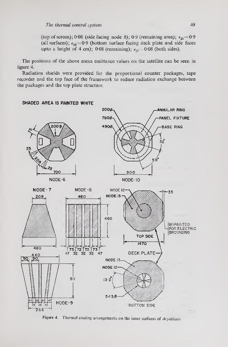
The thermal control system 49
(top of screen); 0-08 (side facing node 8); 0-9 (remaining area); e15=0-9 (all surfaces); e16=0-9 (bottom surface facing deck plate and side faces upto a height of 4 cm); 0 08 (remaining); e17 0 08 (both sides).
The positions of the above mean emittance values on the satellite can be seen in figure 4.
Radiation shields were provided for the proportional counter packages, tape recorder and the top face of the framework to reduce radiation exchange between the packages and the top plate structure.
SHADED AREA IS PAINTED WHITE
PAINTED FOR ELECTRIC GROUNDING
NODE-7 NODE -8
480
m ////
P i %
i
NODE I
NODE 13
480
t 73 | 72 f 72 f 73 f 47 32 32 32 47
NODE
NODE I
5450
NODE-9
TOP SIDE
1470
DECK PLATE
BOTTOM SIDE
Figure 4. Thermal coating arrangements on the inner surfaces of Aryabhata
50 H N Mur thy et a l
A 6-5 mm thick fibreglass insulation ring was provided between the bottom shell and the deck plate to minimise conduction between them.
The chemical battery was thermally isolated from the deck plate by four 8 mm thick fibreglass insulation spacers.
The fibreglass insulation spacers were used between the top plate and shield and between the shield and the proportional counter package itself to minimise conduc¬ tion between the top plate of the structure and the proportional counter package.
4. Provision of thermal control system
The required emittance values on various surfaces were obtained by suitable treat¬ ment to the structure. For the outside surface of the satellite a flat absorber enamel AK-512 black was applied. For the surfaces inside the satellite, various mean emittance values were achieved by a combination of polished and enamel AK-512 white painted areas. The areas to be coated and polished were calculated based on the emittance value of the mechanically polished surface (e=0-08) and the emittance value of the enamel AK-512 white paint (e —0-9). The thermal coating arrangement for the inner surface of Aryabhata is given in figure 4.
To provide suitable strength between the structure and the enamel coatings, the surfaces were degreased with trichloroethylene, anodised and cleaned with benzene before apolication of the coatings. The coatings were applied in layers of 20/x
thickness and cured in the atmosphere before assembling the satellite systems.
5. Verification of the thermal design
It was felt that the theoretical thermal design of Aryabhata could be verified and an overall apprehension of the possible temperature variations due to thermal load regulation could be obtained by testing a thermal model of the satellite in a thermo- vac chamber. A 0-4 size model of Aryabhata, preserving the material, geometrical configuration and surface properties was made and tested in the thermovac chamber. The model was fabricated using the thermal similitude relations. The heat transfer phenomena which were considered while deriving the similitude relations are solid conduction, conduction across joints, internal heat generation sources, change in internal energy, emitted and absorbed radiations. A vacuum of 10~5 torr and cold shroud temperature of— 50°C were maintained in the test chamber. The thermal loads for the skin nodes and the internal subsystem nodes were simulated by using conformal heaters and dummy boxes with resistance heaters respectively. Only steady-state heat balance tests were conducted with averaged thermal load over an orbit. Three orientations of the satellite spin axis with the sun vector, both in the maximum and minimum percentage illumination conditions, were considered for the average load simulation for the nodes. Analyses of the observed results were carried out taking into account all the deviations from the similitude requirements in the model fabrication, load simulation and the errors introduced due to uncer¬ tainties in the material properties. It was found that the observed temperatures agreed within ± 7°C for the internal nodes and within i 20°C for the skin nodes of the satellite.

The thermal control system 51
6. In-orbit performance of the thermal control systems
To monitor the health of the satellite and to evaluate the performance of the thermal control system, 16 temperature sensors were fixed on the satellite structure and on the various boxes of the subsystems. A list of these temperature sensors and the observed temperature ranges during the first six months are given in table 2.
It can be seen from table 2 that the thermal control system has maintained the temperature inside the satellite within the specified limits of 0°C and 40°C, the only exception being the temperatures of the chemical battery and the tape recorder which experienced —1°C and — 5°C respectively for short periods of time.
6.1. Comparison of the calculated and observed temperature values
For purposes of comparison, the temperature distribution of the satellite was calculated for the actual orbit conditions (orbit parameters, sunlit period and spin axis orientation). These calculated temperatures are compared with the observed values. A graphical representation of the comparison is shown in figures 5 a, b and c. From the figures, the following conclusions can be drawn.
(i) For the battery and the transmitter, the observed temperatures closely match with the calculated values.
Table 2. Details on temperature sensors
Sensor number Location Temperature range experienced
Solar cell panels
SN 3003 Bellyband solar panel — 30°C to 30°C SN 3005 Bottom octagonal solar panel —63°C to 110°C
Structural panels
SN 3007 Top octagonal structure panel — 35°C to 85°C SN 3009 Top inclined structure panel — 30°C to 63°C SN 3011 Bellyband structure panel — 16°C to 30°C SN 3013 Bottom inclined structure panel — 15°C to 36°C SN 3015 Bottom octagonal structure panel -47°C to 88°C
Electronic subsystems
SN 3002 Tape recorder (TR-11) -5°C to 37°C SN 3004 Chemical battery -1°C to 28°C SN 3016 Transmitter — 3°C to 22°C SN 3008 X-ray experiment box, EX-11 -1°C to 24°C SN 3014 Neutron gamma experiement box,
Ex-21 0°C to 24°C SN 3012 Ionospheric experiment box, EX-31 — 2°C to 23°C SN 3001 Control box-2, PW 32 4°C to 35°C SN 3010 X-ray experiment box
Spin-up system (proportional counter) EX-12 - 14°C to 51°C
SN 3006 Gas bottle (B-l) -18°C to 40°C

52 H N Murthy et al
0 200 400 600 800 1000 1200 1400
orbit number
0 200 400 600 800 1000 1200 1400
orbit number
Figure 5. (a) The calculated and observed values of the temperature are plotted as a function of orbit number for chemical battery and transmitter
(ii) The tape recorder temperature is consistently higher than the calculated
values upto the 1250th orbit, after which the observed temperatures are
consistently lower than the calculated values. The difference may be due to
(a) conduction heat transfer between the tape recorder and shield,
(b) lumping of the thermal mass of the tape recorder and its table for
calculation purposes, and
(c) error in radiation exchange factors.
During the initial phase, the spin axis was almost directed towards the sun. Then
a negative gradient existed between the tape recorder shield and the tape recorder
table. Therefore, in the beginning, the temperature of the tape recorder was higher
than the calculated value, which is the mean temperature for the tape recorder and
its shield. The conduction from the heat shield further increased the difference. How¬
ever, as the angle between the spin axis and the sun vector increased, the temperature
reduced until its difference became zero at about the 1250th orbit and then the obser¬
ved temperature became lower than the calculated values because the direction of the
temperature gradient in the tape recorder assembly was reversed. The temperature
calculations for four representative orbits were made alter considering points a and c

The thermal control system 53
0 200 400 600 800 1000 1200 1400
orbit number
0 200 400 600 800 1000 1200 1400
orbit number
Figure 5. (b) Calculated and observed values of the temperature plotted as a function of orbit number for tape recorder and gas bottles
and the results are marked on the temperature curve for the tape recorder. These results show an improved match with the observed temperature values.
(iii) The calculated temperature of node 14 (the subsystems housed within the framework) is in between the observed temperatures of various subsystem packages. The temperature of the power regulator is highest because of the presence of a power package near this package which dissipates nearly 20 W of heat. The lowest temperature of the ionosphere experiment box is similarly explained by no dissipation in the box, its nearness to the deckplate and its distance from the stack of the power boxes.
(iv) The temperature of the proportional counter package is consistently higher than the calculated values in the beginning and the difference drops to zero
Pro. C—4

tem
pera
ture
(°C
) te
mp
era
ture
(°C
)
54 H N Murthy et al
0 200 400 600 800 1000 1200 1400
orbit number
0 200 400 600 800 1000 1200 1400
orbit number
Figure 5. (c) Calculated and observed values of the temperature plotted as a function of orbit number for node-14 and EX-12 (x-ray astronomy package)
by the 1250th orbit. This difference is explained by the fact that for the calculations the top face of the package was assumed to have nolieat exchange with space due to the presence of the mylar shield. In fact, the removal of this shield before the launch invalidated the assumption. This explains the behaviour of the temperature difference between the observed and the cal¬ culated values with time. The calculations were made considering the absence of the radiation shield for four representative orbits, and the results marked on the temperature curve show an improved match with the observed tem¬ perature values.
(v) The gas bottle temperature differs considerably from the calculated values, but it closely matches with the mean temperature values for node 11. For calculation purposes, it was assumed that the gas bottles do not have any conduction with node 11. But the observed data proved that it was not so.

The thermal control system 55
7. Conclusions
The passive thermal control system designed and fabricated for Aryabhata performed satisfactorily during the orbital phase. The observed temperatures of most of the subsystems are found to be in good agreement with the predicted values. The small deviations in the case of the temperature of the tape recorder and the gas bottles can be attributed to simplifying assumptions made in preparing the input for the thermal calculations.
Acknowledgements
The authors are grateful to Prof. U R Rao for his constant encouragement and interest during the course of this work. Thanks are due to the authorities of the Computer Centre, Indian Institute of Science, Bangalore, for the running of various programmes and to the Process Shop of the Helicopter Factory, Hindustan Aeronautics Limited, Bangalore for surface treatment of the various models of Aryabhata.
The active participation of Messrs R Ponnappan and P K Abraham in the completion of this work is appreciated. The authors are also grateful to Shri Varadarajulu for providing thermal sensors for the measurement of temperatures.
List of symbols
A surface area of an isothermal node (cm2)
AFa effective surface area for albedo input (cm2)
AFe effective surface area for earth radiation input (cm2)
APs effective surface area for solar radiation input (cm2)
A\ mean area for conduction (cm2)
Ac nominal area of contact for conduction (cm2)
C thermal conductance between nodes (W/°C)
/ radius at contact points (cm)
h length of conduction path (cm)
Fij shape factor of node / with respect to node j
P internal heat dissipation (W)
qa albedo radiation input (W/cm2)
qe earth radiation input (W/cm2)
qs solar radiation input (W/cm2)
R average value of solar reflectance of the earth
T temperature of an isothermal node (°K)
t time (seconds)
W thermal capacity of an isothermal node (joules/°C)
ac coefficient of heat transfer through contact (W/cm2 °C)
56 H N Murthy et al
ag coefficient of heat transfer through gas (W/cm2 °C)
ak coefficient of thermal contact conductance (W/cm2 °C)
ar coefficient of heat transfer by radiation (W/cm2 °C)
as absorptance of a surface for solar radiation input
/? angle between normal to a surface and spin axis of the satellite
y angle between the direction in which projected area is required and the spin- axis of the satellite
e emittance of a surface in infra-red radiation spectrum
ee absorptance of a surface for earthshine input
eu absorption factor of node i with respect to node j
P reflectance for infra-red radiation
rj ratio of actual area to nominal area
A thermal conductivity of material (W/cm °C)
Afc equivalent thermal conductivity (W/cm °C)
cr Stefan-Boltzmann’s constant (5-67 Xl0-12 W/cm2 °K4)
<f>, ifj angles defining the position of the earth element relative to the earth-satellite
co solar aspect angle
References
Bernier R E, Hoffman R H, Timmins A R and Powers E I 1965 NASA TN D-2614 Finch H L, Sommerville D, Vogt R and Bland D 1968 NASA TR R-278 Fontana A 1967 NASA TN D-4133 Hallman R, Conover M, Morrison E and Neilson G 1970 J. Spacecr. Rockets 7 126 Kreith F 1962 Radiation heat transfer for spacecraft and solar plant design (Scranton: International
Textbook Company) Miller P L and Wiebelt J A 1967 Prog. Astronaut. Aeronaut, ed. G B Heller (New York: Academic
Press) Vol. 20 Oshima K and Oshima Y 1968 ISAS Rep. 419 Semple E C 1968 Radio Electron. Eng. 35 1

Attitude and temperature sensors
G A KASIVISWANATHAN,* V P V VARADARAJULU, P R VENKATESWARAN and T K ALEX ISRO Satellite Centre, Peenya, Bangalore 560 058 ♦Present address: INS AT Project Office, 10-A, Kasturba Road, Bangalore, 560 001
MS received 28 April 1977; revised 17 December 1977
Abstract. Aryabhata was a spin-stabilised satellite. Attitude determination was required for the evaluation of the stabilisation system and for scientific experiments. Temperature sensors were required for the performance evaluation of the onboard systems and of the thermal control system. A detailed description of the sensors used for these functions in Aryabhata is given.
Keywords. Attitude sensors; magnetometer; spin angle clock; spinning satellite.
1. Introduction
Aryabhata was spin-stabilised, the spin being imparted after injection into orbit by gas jets. No control on the spin axis orientation was attempted. A nutation damper was used to damp out initial coning motions introduced at the time of im¬ parting spin. Solar aspect sensors and a triaxial magnetometer were used onboard for attitude reconstruction of the spin axis. A spin angle clock was used for sectoring the scan field of the equatorially-mounted x-ray experiment package. A set of temperature sensors placed at various locations of the satellite provided informa¬ tion on the thermal behaviour of the satellite. Details of the different sensors follow.
2. Solar sensors
2.1. Solar aspect sensor
Since the spin was imparted after separation and no control of spin orientation was attempted, the solar aspect angle (the angle between the spin axis and sun-satellite line) could be anywhere between 0° and 180°. This required the sensor range to be 0°-180°. A 7-bit resolution which corresponds to 1-5C was used to meet the require¬ ment of the scientific experiments. The sensitive field of view of the photodetector dictated the use of two separate sensors mounted 90° apart to cover the range.
As the variation in the solar aspect angle is negligible for the duration of a few rotations of the satellite about its own axis, it was considered sufficient to acquire the data once in every rotation. Since synchronisation of the telemetry readout with data acquisition was not possible due to variations in the spin rate, the data
57

58 G A Kasiviswamthan ct ctl
buffer memory -8 bit
obtained when the sensor faced the sun were stored in a buffer memory for telemetry readout, and reset a quarter spin period before the next acquisition. Figure 1 shows the principle of the sensor (Albus 1961). Seven photo-detectors were placed behind a coded mask. For every step of the elevation angle, there is a unique combination of the seven photo-transistors that will be energised. The outputs of these detectors were used to set seven flip-flops fashioned out of 14 NAND gates, serving as the memory. The output of the flip-flops were read by telemetry. A short time before sun acquisition, these flip-flops were reset by a pulse generated by the spin clock to wait for an updated value. The output amplitude was 9 V for the ‘ one ’ state and less than a few mV for the ‘zero’ state. The current consumption was less than 5 mA when all the sensors are lighted at 126° aspect angle. A resistance in series with the output provided circuit protection during test and integration. This enhanced output impedance was acceptable to the complimentary symmetry metal-oxide semicon¬ ductor (CMOS) input impedance of the interfaces. As noted earlier, the sensor is a dual unit, each unit covering 90°. The sensor body was fabricated from aluminium. All surfaces were painted dull black to reduce local reflections. The masks were photo-etched nickel-plated copper sheets.
The detectors were photo-transistors, fashioned out of PNP silicon transistors of a small chip area. The casing was opened and the transistors were potted with optically transparent epoxy. This approach was necessary as the available com¬ mercial photo-transistors had a large chip area and were of the NPN type. During fabrication of the sensors, each photo-detector array was aligned under a microscope to ensure collinearity.
2.2. Solar transit sensor and spin clock
The x-ray astronomy experiment onboard Aryabhata has a scintillation telescope looking through the belly-band of the satellite. X-ray events had to be assigned different angular ‘ bins ’ in the belly-band. For this purpose, the azimuth plane was

A ttitude and temperature sensors 59
ref. pulse
Figure 2. Scheme of operation of spin clock
divided into 128 sectors with a spin angle clock. Four solar transit sensors were used to provide reference pulses for the spin clock every quarter rotation. The four transit sensors were placed on the outer shell in the X, —X, Y and — Y directions of the satellite. Each sensor consisted of photo-transistors placed behind a slit mask, the slit direction being parallel to the spin axis. Two detectors were used for each sensor. The field of view and fabrication details are similar to the aspect sensor. During sun transit the photo-detectors produce a negative pulse to provide the reference pulses for the spin clock.
Figure 2 shows the operation of the spin clock. (Bartley et al 1967). Output pulses from a stable clock were counted in counters A and B, of 5-bit and 8-bit lengths respectively. Whenever a transit pulse was fed, the contents of B were transferred to register R and both counters were reset after a small delay. The clock pulses were also fed to another counter C which was compared with the content of the register R. The comparator output was thus a pulse train with a frequency ns (but for the residue in the counter A at the time of resetting), where n is the capacity (maximum content) of the counter A and 5 the frequency of the reference pulses. If we consider T as the number of clock pulses available between the two successive reference pulses, then T nm + r where n = capacity of counter A, m — number of counts transferred from B to register R and r residual counts in A at the time of transfer (always <ri).
The comparator operation, combined with the resetting of C with its output, i§ equivalent to division by m and thus the output pulses from the comparator during the period will be (nm-\-r) A- m ~n.
It will be seen that as the spin decays, the residue r will slowly increase to value n which occurs when the period T is an exact multiple of n. But now the content of

60 G A Kasiviswanathan et al
J_1 ! j
inn_lL 01 2 3 3132
sun ref- pulse
uncorrected sector pulses
v cC residue integrator output
vm— i i * • i * i . •
0 12 3 31 32
fast ramp
corrected sector pulses
Figure 3. Scheme of correction for spin clock
register R will be incremented by 1 count due to overflow from A and the division will now be with m+l instead of m, thus giving an output pulse.
The time error of each output pulse progressively increases by an increment of r/n for each step; in this scheme correction for this residue was introduced by progressively shifting the occurrence of these pulses. Figure 3 illustrates the principle.
Referring to figure 2, the residue in the counter A, was converted to an analog voltage with a D/A converter which follows register R into which the value of the residue was transferred. This analog voltage was fed to an integrator to give a ramp output, which was periodically reset by the (sun) reference pulse. The pulses from a comparator were used to reset another ramp generator periodically. The two ramps were fed to an analog comparator. The corrected sector information was obtained from this comparator output. The 128 corrected pulses in each rotation were fed to a 7-bit counter to provide the azimuth. This counter was preset to the proper value by a preset matrix whenever the reference pulse was available from one of the four transit sensors.
The 7-bit parallel output from the counter was fed to the x-ray experiment for onboard processing. The two most significant bits were obtained directly from the sensors, and the remaining 5 bits were taken from the sector generator for attitude purposes. This scheme provided a facility to monitor the functioning of the sensors and spin clock electronics separately. A pulse from the spin clock preset matrix was used for resetting the solar aspect sensor.
S. Triaxial magnetometer
The geomagnetic field was chosen as the second reference vector for attitude deter¬ mination and a triaxial magnetometer of the flux gate type was used. Since the total field for the nominal satellite orbit is of the order of 35,000 gamma, the range of the

Attitude and temperature sensors 61
(0)
input voltage current
(b) Figure 4. Circuit diagram for magnetometer
magnetometer was set at J-45,000 gamma to accommodate the local field due to the satellite. The output range of 0 to +5 V was specified by the analog input require¬ ments of the telemetry system. This analog voltage was digitised by the telemetry system before transmission.
In order to evaluate the spin rate of the satellite, the sampling of the magneto¬ meter data was performed at 4 samples/s. Even though this corresponds to only 2-5 samples/rotation at the maximum spin rate of 90 rev /min, in view of the spin rate decay, a higher sampling rate was available at the lower spin rate; as many as 24 samples/rotation were available at the lowest acceptable spin rate of 10 rev/min.
The three sensor coils, orthogonal to each other, were mounted in a separate package away from the sensor electronics. The sensor was placed on the top deck plate free from the disturbing field of all the lower deck-plate mounted electronic packages. The basic circuit (figures 4a, b) of the peaking type magnetometer was an LCR circuit, to which positive and negative voltages were applied, alternately. The inductance L was a small saturable reactor which required a saturating field of the order of the geomagnetic field. This external field changes the point at which satu¬ ration occurs and this, in turn, alters the peak of the current pulse (voltage across R).
The effect on the peak current in the circuit by the external field impressed voltage V
is shown in figure 4b.

62 G A Kasiviswanathan et al
3.1. Circuit details
The oscillator, built with CMOS NAND gates, was temperature-compensated. The oscillator frequency was 5 kHz. This frequency varied only by 1 % with a change in temperature of — 10°C to +50°C. The oscillator output was fed to a bi-stable to divide the frequency to half its value and to get the two identical pulse trains displaced by 180° for driving the crossover switch, which was used to reverse the current in the sensor coil periodically. By this circuit, the voltage across the resistance R was always in the form of positive pulses. The peaks of the alternate pulses across R were separately detected. A unique phase sensitive detector was used. This consisted of a single emitter follower followed by two CMOS switches. This gave a high input impe¬ dance and high stability for differential signals. The two detector outputs were fed to an instrumentation type amplifier. This configuration provided high input impedance for both the inputs and avoided loading of the detectors. The input impedance seen by two detectors were equal. The amplifier gain was approximately 600.
To improve linearity and to reduce the variations of the output due to temperature, a feedback circuit was used. The output was fed to the feedback coil and this restricts the swing of the operating point on the B-H curve. The magnetometer was calibrated using three pairs of Helmholtz coils which give a highly uniform field in a sufficiently large space. Two pairs of the coils were of 1000 mm diameter and the third pair was of 500 mm diameter.
A calibration coil was built in the sensor coil package. By passing a known current into this coil, calibration sensitivity was checked at every stage of qualifi¬ cation.
3.2. Magnetic cleanliness
Since the field contributions of the subsystems and components were not available during the early design phase, every effort was made to keep the satellite as magnetically clean as possible. The different phases in which this was achieved are discussed below.
3.2a. Hardware testing
The hardware used in satellite integration was screened magnetically to avoid magnetic contamination. The hardware was exposed to a high field of the order of 25 gauss in a Helmholtz coil system and the maximum radial field created by it was measured. If the field disturbance at the magnetometer location was less than a specified limit (2 gamma), the hardware was accepted. Relays, used in the telecom¬ mand and power systems were arranged in different configurations and the radial field was plotted in three orthogonal planes in each configuration. The configuration giving the minimum field disturbance at the magnetometer was selected.
The currents flowing in various electronic systems give rise to magnetic fields. To minimise the field due to these currents, the leads from the power system to the electronic system were twisted in pairs and the power system was grounded to the satellite structure at a single point.
Attitude and temperature sensors 63
3.2b. Solar panel testing
The resultant magnetic field at the magnetometer due to the current flowing in the solar panel was measured. The components of the magnetic moments of each solar panel were determined by illuminating the panel in the sunlight and recording the radial magnetic field. These components were converted into the magnetic field components at the magnetometer location, knowing the position of the solar panel and its orientation.
3.2c. Subsystem testing
Most of the electronic subsystems were placed on the lower deck plate of the satellite. Each electronic subsystem package, after completion of the environmental tests, was evaluated to determine its magnetic field contribution at the magnetometer. The magnetic test for the subsystem consisted of determining the components of its magnetic moment for the following ‘ magnetic states initial perm (initial magnetic state of subsystem); post 25 gauss magnetisation; post demagnetisation.
4. Temperature sensors
To keep the various subsystems in the satellite within their respective operating temperature ranges, a passive thermal control technique was used. In order to monitor the general health of the satellite, temperature sensors were fixed on some subsystem packages and at important locations on the satellite structure. Out of the several standard methods available, it was found that a thermistor would be the best choice as a sensing element for temperature measurement since by proper design, one can obtain tens of milli-volts change in the output per unit temperature change. So, further amplification of the output is not necessary, whereas amplification is required to get the same order of sensitivity in the case of a thermocouple or a resistance thermometer. After deciding to use thermistors as temperature sensors, it was found that, in contradistinction with a constant current mode of operation, the constant voltage mode enabled coverage of a wide temperature range with the same order of sensitivity. The optimum supply voltage and series resistance were determined to cover the maximum temperature range with the required sensitivity.
4.1. Specifications
Temperature sensors with the following specifications were used.
Temperature range of sensor ; — 70°C to -f 120°C
Accuracy/repeatability : ± 2°C in the range—20°C to + 80°C; ± 4°C below —20°C and above + 80°C
: 25S • . Response time

64 G A Kasiviswanathan et at
Each temperature sensor consisted of a space-qualified thermistor encapsulated in a metal housing. The weight of each sensor was 2-3 g. The sensors were fixed on the packages with thermally conductive epoxy.
The electronics package supplied the proper biasing voltage to the respective temperature sensors. The bias voltage was 5 V± 005 V in the temperature range —20°C to +60°C. A voltage proportional to the temperature of each sensor was developed across its series resistance and was sampled by the telemetry system.
4.2. Calibration
A set-up for calibrating these sensors consisted of two units. One unit calibrated the sensors above room temperature. The system diagram is shown in figure 5a. The range of temperature that could be controlled extended from ambient to + 120°C. The stability and repeatability of the set-up were better than 001°C and 0-2°C respectively.
The unit to calibrate the sensors below room temperature is shown in figure 5(b). The chamber could be controlled to any temperature in the range of room temperature down to — 70°C. Its repeatability was 0-5°C and stability 01°C. To ensure high reliability, each sensor was assembled with the utmost care and calibrated several times before and after mechanical qualification tests with the help
(0)
(b)
Figure 5. Calibration set-up for temperature sensors

Attitude and temperature sensors 65
of the calibration set-up. A voltage-temperature graph was derived for each sensor. A typical graph is shown in figure 6.
5. Alignment of sensors
In order to carry out the alignment, ‘ bench marks * showing the reference axes were provided on the sensors. Figure 7 shows the solar aspect sensor with the above
Figure 6. A typical calibration curve for temperature sensor.
Figure 7. Solar aspect sensor with alignment marks.

66 G A Kasiviswamthan et al
Figure 8. Magnetometer with alignment pins.
provision. The solar aspect sensor had two reference lines P and Q marked on the
body. Line P represented the Z-axis of the sensor and was parallel to the Z axis
(spin axis) of the satellite. Line Q normal to line P, was along the X- Y plane of the
satellite. In the transit sensors, the slit direction was the principal axis and was to
be aligned along the Z-axis. The magnetometer had three alignment pins attached
to the mounting surface. These pins projected through the top plate of the satellite.
The top of the pins defined the X- Y plane. Pins O and X defined the X direction
and O and Y defined the Y direction (see figure 8). The satellite was mounted on a
spin table with angular readout of 0T° accuracy. The spin table surface was kept
horizontal using a spirit level.
A theodolite was set at a comfortable distance from the spin table. The vertical
cross hair of the theodolite was first checked and aligned with a plumb line.
5.1. Solar aspect sensor
The satellite was rotated with the help of the spin table until the sensor was seen
through the theodolite. Line P was adjusted for verticality. The satellite was
rotated through 90° to get the line Q in view of the theodolite and the sensor
mounting was adjusted for level as checked with the theodolite horizontal cross wire.
The two operations of the line P and Q adjustments were repeated a few times.
5.2. Transit sensor
Immediately after the alignment of the solar aspect sensor, the transit sensor on the
same face was brought into the field of view of the theodolite. When both half slits
appeared as a continuous line, the sensor was facing squarely on the theodolite.
After taking a reading on the spin table corresponding to this sensor, the satellite on
the spin table was rotated through an exact angle of 90° and the corresponding sensor
mounting was adjusted. The same process was repeated with sensors on the other
faces also.
5.3. Magnetometer
The magnetic sensor was fixed on the top deck of the satellite. After the assembly
of the top and bottom shells, there was no provision for adjustments of the magnetic

67 Attitude and temperature sensorsJ
sensor. Hence, only a measurement was made of the misalignment. The Z-axis
alignment was measured with a calibrated spirit level on the top of a smooth glass
plate placed over the alignment pins. ... : :
The reading on the spin table corresponding to the positions of the pins O and X
along the line of sight of the theodolite was noted. After turning the satellite on the
turn table to bring the O and Y pins along the line of sight, a second reading was
taken. The two readings were repeated to reduce random errors. From these
readings the alignment errors were calculated.
6. Attitude determination
The attitude of Aryabhata was determined using the triaxial magnetometer and the
solar aspect sensors (Kalweit 1969). The triaxial magnetometer gives the orientation
of the satellite axes with respect to the geomagnetic field while the solar sensors give
the angle with respect to the sun-satellite vector.
From the three components of the geomagnetic field (Hx, Hy, Hz) the angle d,m
between the spin axis and the geomagnetic field vector is given by:
cos 6zm = HJ{Hxs + Hp, + Hpf'K
The solar aspect sensor measures the angle 6ZS between the sun-satellite vector and
the spin axis. The spin axis lies along one of the lines of intersection of the two
cones generated about the sun-satellite vector and the geomagnetic field vector with
the half cone angles of 9ZS and 8zm respectively. The ambiguity between the two
lines of intersection is resolved using the expected attitude from the launch conditions
or the apparent variation of attitude with respect to time.
The telemetry data were first decoded and the sensor outputs were separated. The
onboard time code generator output was decoded and real time was allotted to each
sensor output. Whenever necessary, the onboard time was corrected using the
ground station time.
The telemetered data were converted to actual magnitude using the sensor cali¬
bration data. The satellite position was calculated as latitude, longitude and altitude
using the tracking data and orbital calculations. The geomagnetic field directions
at the satellite position were calculated using the spherical harmonic field models.
These directions were transferred to celestial coordinates using sidereal time. The
sun’s direction was also computed using ephemeris data. Using the above infor¬
mation, the attitude in celestial coordinates with respect to time was computed.
Owing to an initial malfunction in the spin-up system, Aryabhata was tumbling
for the first 45 orbits without spin stabilisation. The sun sensors designed for a
spinning mode were not helpful during this phase. But, as the nature of tumbling
was one of slow spin (about another axis), rough attitude determination was possible
during this phase also. The triaxial magnetometer output was used for this phase.
Using a short-term approximation as a spinning satellite about the new axis, the
attitude was reconstructed in a piece-wise fashion. The single solar aspect reading
obtained during this phase, together with the temperature distribution of the surface
panels, helped to resolve the ambiguity.

68 G A Kasimwanathan et at
7. Conclusion
The attitude and temperature sensors designed for Aryabhata have worked through
transport, launch and orbit environment and performed to specifications. Attitude
and temperature profiles could be computed successfully from the telemetered data.
Acknowledgements
We are grateful to Prof. U R Rao for guidance throughout this work and
acknowledge the enthusiastic technical support provided by Messrs S S Avalaskar,
K Kanakaraju and S B Gupta.
References
Albus J S 1961 Digital Solar Aspect Sensor NASA TN-D-1062 Bartley W C, McCracken K G and Rao U R 1967 IEEE Tran. Aerosp. Electron. AES-3 No. 2 230 Kalweit C C 1969 ESRO I Attitude measurement system ESRO TN-99 (ESTEC)

The telemetry system
D V RAJU, R K RAJANGAM, P S RAJYALAKSHMI,
C N VENKATESHAIAH, R SESHAIAH, V NALANDA,
S R NAGARAJ and R SIVASWAMY ISRO Satellite Centre, Peenya, Bangalore 560 058
MS received 16 April 1977; revised 3 November 1977
Abstract. This paper describes the telemetry system employed in Aryabhata. The telemetry link provides a means for monitoring diagnostic and other parameters for efficient and controlled operation of the satellite besides transmitting data per¬ taining to the three scientific experiments. The design specifications and details, qualification tests and in-orbit performance of the telemetry system are also described in this paper.
Keywords. Satellite telemetry; pulse code modulation; sub-carrier oscillator; change¬ over system; premodulation filter; analog-digital converter.
1. Introduction
The function of the telemetry system was to accept the data pertaining to the
performance of various spacecraft systems and to multiplex it into a form suitable
for transmission to the ground via the telemetry transmitter. Thus, the encoder
which process the data was interfaced with various data transducers, sensors
and signal conditioners at its input and the telemetry transmitter at its output.
Commensurate with the established mission objectives, the telemetry data require¬
ments were analysed on the basis of two major functional areas; (i) diagnostic and
spacecraft status data necessary for efficient and controlled operation of the space¬
craft, (ii) scientific experiment data. Diagnostic and spacecraft status data included
information on the operational parameters of the power, thermal, attitude and
command systems. These were voltages, currents, temperatures, command verifi¬
cation and telemetry calibration signals in analog form whose levels range from
0 V to 5 V and digital form of either 0+0-2 V or 9 V + 0-5 V.
Information from all the three scientific experiments onboard Aryabhata, viz.,
(i) solar neutron and gamma rays, (ii) ionospheric parameters and (iii) x-ray
astronomy, consisting of both digital and analog information, was transmitted
along with the housekeeping and technological data.
For obtaining increased data coverage, in addition to the real time data trans¬
mission, the satellite was also designed for operation in the storage mode. In the
latter mode, magnetic tape recorders were used to store 40 min of NRZ data at 256
bits/s and transmit at 10 times the recorded speed, i.e., at 2-56 kbits/s, both record
and playback operations being controlled by ground commands.
To meet the accuracy requirements and to provide capability for handling various
forms of data, a time multiplexed pulse code modulation (PCM) system was chosen.
69
Pro (C)—5

70 D V Raju et al
In order to avoid the catastrophic failure of the satellite mission due to any mal¬
function in the telemetry system, a parallel redundant system, including an additional
tape recorder, was provided which could be switched on by using ground commands.
The system utilised a 128 word, 8 bits per word format. The PCM signal frequency
modulates a 22 kHz i 7-5% subcarrier which was given to the transmitter for phase
modulation of the main carrier.
2. Design philosophy
Due to severe constraints on power and weight, all the digital subsystems were
designed using complementary symmetry metal oxide semiconductor (Cosmos) inte¬
grated circuits, whereas, the analog subsystems such as comparators, pre-modulation
filters and bandpass filters were designed using IC operational amplifiers. Wherever
close tolerance and extreme stability were demanded, metal film resistors of 0-5%
and 1 % tolerance with 20 ppm/°C and highly stable Mylar capacitors with low
leakage were used.
Pulse code modulation telemetry systems have come into wide usage in the last
few years for all space applications. For applications requiring high accuracy
(better than 1 %) or the sampling of large number of channels of varying
characteristics, handling of both analog and digital signals, flexibility as to number of
channels and their sampling rates, capability of transmitting data of high accuracy
with little or no degradation in the RF link and generally superior characteristics of
information efficiency and noise immunity in the RF links, the PCM system offers
net advantages over other competing modulation schemes.
A PCM system with an accuracy of better than 1 % was chosen to transmit
both the house-keeping and scientific information. The overall specifications for
the telemetry system are listed in table 1.
3. Design details
The telemetry system consists of two PCM encoders, two tape recorders, four pre¬
modulation filters (PMFs) and two subcarrier oscillators (SCOs), the block schematic
of which is shown in figure 1. The encoder outputs —PCM, its complement PCM),
and the clock—were connected to the tape recorder through an encoder changeover
switch and buffers Bls B2, B3. In the real time mode, the PCM data would be
connected to the SCOs through the 256 Hz PMFs and a PMF changeover switch.
The output of either SCOl or SC02 could be coupled to the transmitter by the com¬
mand D. In the playback mode, data recorded for 40 min would be played back in
4 min and connected to the SCOs through buffers and 2560 Hz PMFs.
Command A switches the system from one system/subsystem to the other
(redundant) and command B switches the system from real time to playback and
vice-versa. Also, an onboard timer switches the system from playback to real time
mode after 5 min of playback operation. The encoder consists of a multiplexer, an analog-to-digital converter (ADC), a
digital interface unit (DIU), a parity bit generator, frame and subframe sync code
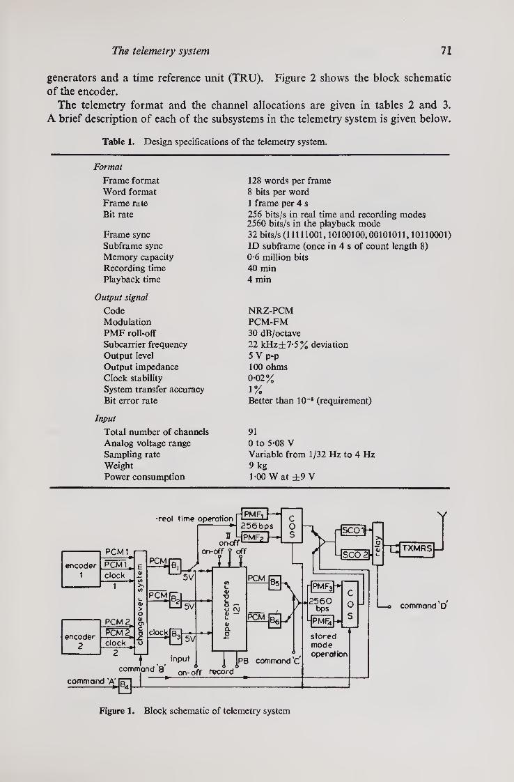
The telemetry system 71
generators and a time reference unit (TRU). Figure 2 shows the block schematic
of the encoder.
The telemetry format and the channel allocations are given in tables 2 and 3.
A brief description of each of the subsystems in the telemetry system is given below.
Table 1. Design specifications of the telemetry system.
Format
Frame format Word format Frame rate Bit rate
Frame sync Subframe sync Memory capacity Recording time Playback time
Output signal
Code Modulation PMF roll-off Subcarrier frequency Output level Output impedance Clock stability System transfer accuracy Bit error rate
Input
Total number of channels Analog voltage range Sampling rate Weight Power consumption
128 words per frame 8 bits per word 1 frame per 4 s 256 bits/s in real time and recording modes 2560 bits/s in the playback mode 32 bits/s (11111001,10100100,00101011,10110001) ID subframe (once in 4 s of count length 8) 0-6 million bits 40 min 4 min
NRZ-PCM PCM-FM 30 dB/octave 22 kHz±7-5% deviation 5 V p-p 100 ohms 0-02%
1% Better than 105 (requirement)
91 0 to 5-08 V Variable from 1/32 Hz to 4 Hz 9 kg 1-00 Wat ±9 V
Figure 1. Block schematic of telemetry system

72 D V Raju et al
Figure 2. Block schematic of encoder
3.1. Multiplexer
The analog signals that originate from various sources within the satellite were time
division multiplexed before encoding the data. The multiplexer consists of (a) a
clock source (b) a programmer (c) analog transmission gates (d) a sample and hold
circuit with associated buffers. The bit rate clock, 256 Hz, was derived from an IC
crystal controlled oscillator of frequency 102-4 kHz. The sequential timing pulses
required for multiplexing were generated by the programmer using ring counters
and NAND gates. The analog transmission gates either transmit the signals to the
output line without distortion or completely block them. Cosmos transmission
gates were employed for this purpose to get practically negligible off-set voltage.
A sample and hold circuit was used to store the multiplexed output while the signal
was being encoded and the multiplexer was seeking the next signal to be converted.
Since in the hold mode the capacitor should not be discharged, a capacitor which
has a very low leakage and which switches with low off-set current was chosen.
3.2. Analog-to-digital converter
The multiplexed analog signals were encoded by the use of the well known successive
approximation type of analog-to-digital converter. The ADC mainly consists of an
analog comparator to compare the input voltage Vjn and the feedback voltage (Ff)
generated by the bit flip-flops and the decoder. The decoder consists of analog
switches to switch the ladder network between a reference and the ground.
The conversion process starts with the most significant bit and successively trying
a ‘one’ in each bit of the decoder and is compared against the analog input. If Vf is
greater than Vin the ‘ one ’ is removed from that bit and ‘one’ is tried in the next
most significant bit. If Vin is greater than Vf, the ‘one’ remains in the bit. At the
end of the process after the LSB is tried, the digital word of the comparator output
is the equivalent of the analog voltage Vin. Figure 3 shows the block schematic of
ADC.

The telemetry system 73
Table 2. Telemetry format
FSC Sun-Sen-II Mag-X Mag-Y Iono
NG NG NG NG NG Mag-X Mag-Y Iono X-ray X-ray X-ray X-ray X-ray Mag-X Mag-Y Iono Mag-Z ID-Sub-Sync HK-Sub-Com (16 Ch) X-ray Mag-X Mag-Y Iono
I II Iono-Sub-Ch Iono-Sub-Ch Sun-Sen-I Command Sun-Sen-II Mag-X Mag-Y Iono
NG NG NG NG NG Mag-X Mag-Y Iono X-ray X-ray X-ray X-ray X-ray Mag-X May-Y Iono Mag-Z Command HK-Sub-Com (16Ch) X-ray Mag-X Mag-Y Iono Command Command Sun-Sen-I Command Sun-Sen-II Mag-X Mag-Y Iono
NG NG NG NG NG Mag-X Mag-Y Iono X-ray X-ray X-ray X-ray X-ray Mag-X Mag-Y Iono Mag-Z Command HK-Sub-Com (16 Ch) X-ray Mag-X Mag-Y Iono
I II Iono-Sub-Ch Iono-Sub-Ch Sun-Sen-I Command Sun-Sen-II Mag-X Mag-Y Iono
NG NG NG NG NG Mag-X May-Y Iono X-ray X-ray X-ray X-ray X-ray Mag-X Mag-Y Iono Mag-Z Command HK-Sub-Com (16 Ch) X-ray Mag-X Mag-Y Iono
Table 3. Aryabhata telemetry channel allocations
Description Analog Digital bits per 8 frames
(32 s) Sampling rate
(Hz)
Words per 8
frames
Bits per 8 frames
(32 s)
Diagnostic and status
Power subsystem 12 — 0 031 12 96 Thermal subsystem 16 — 0 031 16 128 Attitude subsystem
Mag. sensor (a) 2 — 4-0 256 2048 Mag. sensor (b) 1 — 1-0 32 256 Sun sensor (c) — 256 1-0 32 256 Sun sensor (d) — 192 0-15 24 192
Command subsystem (a) 20 — 0-031 20 160 (b) 8 — 0-25 64 512
Communication sub- system (AGC) 2 — 0-031 2 16
Scientific experiments
X-ray astronomy Solar-neutron and
— 1536 1-0 192 1536
gamma ray experiment — 1280 1-0 160 1280 Ionosphere experiment (a) — 1024 4-0 128 1024
(b) 2 — 0-5 32 256
Telemetry
Tape recorder 5 — 0-031 5 40 Frame sync — 256 0-25 32 256 Subframe sync — 64 0-25 8 64 Calibration 6 — 0-031 6 48 Reference time 24 0-031
Total
3 24
8192
Bit rate = 8192/32=256 BPS

74 D V Raju et al
Figure 3. Block schematic of analog-to-digital converter
3.3. Digital interface unit
Digital data from the three scientific experiments and the sun sensors, were available
in parallel form, whereas the encoded analog data were available in serial form. To
have the PCM data in serial form, the digital data were entered into the shift registers
in parallel and shifted out serially, synchronous with the bit rate clock. The syn¬
chronous operation was made possible by resetting the counters in the different
experiments by telemetry bit pulses and word pulses. The serial digital data were
mixed with the encoded analog data at the appropriate time slots.
3.4. Parity bit generator
For the correct interpretation of the received data some kind of check bits are neces¬
sary. For this purpose, an odd parity check was employed. The correct data are
identified by the odd number of ‘ones’ in each word and this type of check would
enable single bit errors, three bit errors, etc., to be detected. Exclusive OR and NOR
gates were used to realise the above function.
3.5. Frame and subframe sync code generator
In order to have proper identification of the data at the ground stations, frame and
subframe synchronising codes were incorporated in the PCM pulse train at ap¬
propriate places. The frame sync code was chosen such that the probability of data
resembling the sync code is the least. The frame sync code generator was developed
using shift registers (32 bits) and suitable logic gates.
ID subframe synchronisation was preferred to recycle subframe synchronisation,
since in ID subframe synchronisation, the identification is transmitted once for each

The telemetry system 75
revolution of the main frame. The main iframe (4 s) was counted by the frame
counter and the counter output was mixed at the appropriate place, with the other
data. The length of subframe is 8 main frames and the ID code has 3 bits.
3.6. Time reference unit
In order to have the time correlation of data, time information was mixed with data
and transmitted. The major frame counter was used as a time reference for the
spacecraft. It is a 21-stage binary counter, that is incremented every major frame
(8 frames) or every 32 s resulting in a capability of a non-repetitive read-out for
approximately two years. By examining the major frame counter and the frame
identifier, spacecraft time can be resolved to 4 s.
3.7. Premodulation filters and subcarrier oscillator
The NRZ-PCM is rich in odd harmonics and the frequency contents are limited by the
rise time of the data only. In order to reduce the r.f. bandwidth, with marginal
degradation of performance, a low pass filter known as premodulation filter was
employed. It is a 6-pole, 3-stage, Bessel type of filter, operating on multiple feed¬
back principle to get (a) maximally flat response, (b) linear phase, (c) final slope
—30 dB/octave, and (d) cut-off frequency equal to the nominal bit rate. Two
such filters were used for real time operation at 256 bits/s and two for stored mode
operation at 2560 bits/s.
The filtered signal frequency modulates a 22 kHz, ^ 7-5% deviation, multi¬
vibrator type of voltage controlled oscillator, followed by a single stage 2-pole, active
bandpass filter.
3.8. Changeover system
Only one of the two systems should be connected to the r.f. link at any one time.
Therefore, changeover systems activated by telecommand were necessary at the
outputs of the various units constituting the systems. There were three changeover
circuits, one each for the encoders, pre-modulation filters and control pulses.
The basic building block of the system is a CD4016 quadrupole bilateral switch.
For reliable operation, two such gates were connected in parallel.
3.9. Tape recorder
The tape recorder used in the Aryabhata mission is of the endless loop type with a
capacity of 06 million bits and a playback to record speed ratio of 10:1. The tape
recorder has 3 tracks on which the 256 Hz clock, data and the data complement were
recorded in parallel. The output levels are the same as the input levels of 5 V^l V
for ‘high’ and 0, or IV for Tow’ logic conditions. Two tape recorders connected
in parallel ensure reliability through redundancy.
The outputs from the encoder changeover switch were connected to both the tape
recorders through appropriate buffers. The outputs of the two tape recorders were
electronically coupled so that only the tape recorder which is in the ‘ on ’ condition
delivers the output to 2560 Hz premodulation filters through buffers. Both the tape

76 D V Raju et al
recorders could be turned ‘ off ’ by the tape recorder ‘ off ’ command and during real time operation, both the tape recorders remain in the ‘off’ condition.
4. Qualification tests
The evolution of the flight packages of the onboard telemetry system has gone through many stages such as the bread-board, engineering (pre-prototype) and proto¬ type models. As the development of these models would depend upon the specifi¬ cations of the components used, the qualification tests and their levels would also vary accordingly. In general, the tests could be divided broadly into three categories, viz. (i) bench tests (electrical), (ii) environmental tests, and (iii) integration tests. In bench tests, the individual packages of the telemetry system were tested for their electrical performance and later all the packages were integrated and tested as a single system.
The packages were subjected to the following environmental tests: (1) cold and hot storage temperature, (2) cold and hot soak temperature, (3) humidity, (4) vibration, shock and (5) thermal vacuum. The packages were checked for their operational performance and for mechanical or electrical damage at various stages in the above tests. The test levels for the prototype were slightly higher than those for the other models used, to test the failure limits for each of the packages. The test levels for each model can be found in another paper on quality assurance aspects for all subsystems.
The onboard tape recorders were tested for fidelity of recording and flutter in the output. The test results revealed that all the models of the telemetry packages have performed well according to the design specifications in both bench and environ¬ mental tests. The telemetry system was integrated along with the other satellite systems and tested for the interface specifications.
5. In-orbit performance
Except for a brief period during the initial stages when the telemetry synchronisation was lost, the telemetry system has performed satisfactorily, both in the real time and playback modes, throughout the entire period of its operation. The problems en¬ countered by the system in various orbits are explained below:
(1) in the latter part of the 17th orbit at Bears Lake, there was no telemetry signal; (2) there was lack of frame synchronisation from 24th through 31st orbits; (3) due to carrier drop-outs there were frequent synchronisation losses from 38th
through 41st orbits; (4) from 42nd to 59th orbits there was no playback data from the tape recorder;
and (5) the time reference signal in encoder-1 advanced by 770 frames from 17th
through 59th orbits.
Except for these initial problems, the system performed well according to the speci¬ fications given in table 4 showing the coding accuracy and figure 4 showing the bit error probability for various orbits and the signal strength respectively.

The telemetry system 77
Table 4. Coding accuracy of A/D converter with particular reference to calibration voltages
Expected calibration voltage counts (BCD) 133 135
Observed counts (BCD) for various orbits 158 171 173 238 355 393 414 437 502 546
0 1 0 0 0 0 0 0 0 0 0 0 0 0
25 ± 1 25 25 25 25 25 25 25 25 25 25 25 25
51 ± 1 51 51 51 51 51 51 51 51 51 51 51 51
77 ± 1 77 77 77 77 77 77 77 77 77 77 77 77
103 ± 1 103 103 103 103 103 103 103 103 103 103 103 103
127 126 127 127 137 127 127 127 127 127 127 127 127 127
Expected calibration voltage counts (BCD) 560 584 590 604 614 708 737 766 772 781 805
0 1 0 0 0 0 0 0 0 0 0 0 0
25 ± 1 25 25 25 25 25 25 25 25 25 25 25
51 ± 1 51 51 51 51 51 51 51 51 51 51 51
77 ± 1 77 77 77 77 77 77 77 77 77 77 77
103 ± 1 103 103 103 103 103 103 103 103 103 103 103
127 126 127 127 127 127 127 127 127 127 127 127 127
-3
signal strength (dBW)
Figure 4. Bit error probability
78 D V Raju et al
6. Conclusions
From the simulation studies conducted to investigate the probable causes of the malfunctions observed, the following results were arrived at.
(1) Whenever—9 V common bus (CB) was affected, intermittent failures in the telemetry link were observed. These failures were associated with only ± 14 V supply lines of solar neutron and gamma-ray (N-G) experiment. When ± 14 V of N-G was found to draw 150 mA as against rated current of 20 mA, on account of failures in d.c./a.c. converter of N-G system, the — 9 V CB was reading + 1 V. This resulted in the complete absence of SCO signal which was similar to the problem in the 17th orbit. Moreover, in that condition, whenever the + 14 EX failsafe operated intermittently, non-locking of frame synchronisation, bit shifts and ID failures were observed resembling the prob¬ lems observed during the 24th to 31st orbits.
(2) The malfunction of the tape recorder was due to the TR-1 signal being ‘ on ’ constantly and not for the required 0-4 s only. By a different sequence of commands in a later orbit, the TR-1 was switched off and TR-2 was switched ‘ on’. The performance of TR-2 has been found satisfactory.
(3) The advancement of time reference signal during 17th-59th orbits may be due to the influence of some spurious signals since there were disturbances in the link during these orbits.
Acknowledgements
The authors wish to express their appreciation for the support extended by Messrs Puttaiah and Ajeet Phadnis who were responsible for the successful qualification of the telemetry system. They would like to thank Prof U R Rao for the encourag- ment given by him. Their thanks are also due to Mrs Annie Nelson and Messrs Rama G Krishna, Narasimhlu Naidu and L Sainath who were responsible for the fabrication of the Aryabhata telemetry system.

The communication system
M K SAHA, V GOPAL RAO, N MANTHIAH, S KALYANARAMAN, M L N SASTRY, D JOHN and M K NAIR ISRO Satellite Centre, Peenya, Bangalore 560 058
♦Present address: INSAT Project Office, Kasturba Road, Bangalore, 560 001
MS received 16 April 1977; revised 25 January 1978
Abstract. The paper discusses the salient features of system design considerations for both uplink and downlink, subsystem details and the in-orbit performance of the communication system for Aryabhata.
Keywords. Link estimate; side band power; noise figure; bit error probability; hybrid coupler satellite communication.
1. Introduction
The communication system for Aryabhata comprises the telemetry link at 137-44 MHz and the telecommand link at 148-25 MHz. The onboard system consists of two telemetry transmitters and two telecommand receivers both coupled to a common antenna via a hybrid coupler unit, which isolates the command receiver from the telemetry transmitter. A stable telemetry carrier frequency of 137-44 MHz is also used for tracking. Telemetry data in pulse coded modulation are frequency-modu¬ lated on a subcarrier frequency of 22 kHz and the composite signal phase modulates the carrier to provide interference-free reception in narrow band carrier tracking systems. The scheme for telemetry transmission is hence PCM—FM—PM. For reliability of the onboard system the principle of parallel redundancy is used. One of the two transmitters is used at any given time for telemetry data transmission whereas the two receivers are used at all times. In the event of failure or malfunction of one transmitter the other is switched on by ground command. The telecommand system that has been chosen is an amplitude modulated system. The received signals at the satellite antenna after detection by receivers are fed to a command decoder which decodes the command information to execute command operations.
As and when ranging information is required, a ground command is initiated to connect the output of the telecommand receiver carrying ranging information for tracking purpose to the input of the telemetry transmitter. While tracking data are collected in this mode, no command operation is carried out: this is because the same telecommand receiver is used for reception of either command information or tracking information. The functional block diagram of the entire onboard communication system is given in figure 1.
79
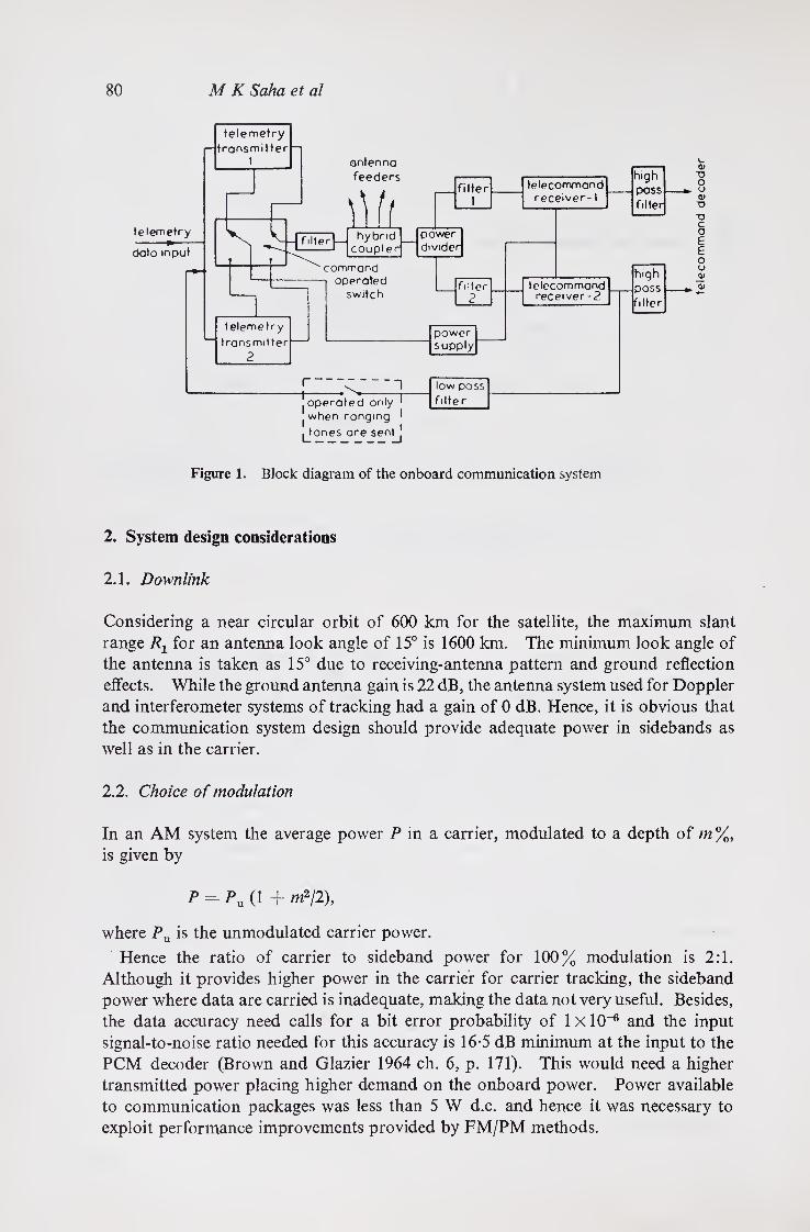
80 M K Saha et al
Figure 1. Block diagram of the onboard communication system
2. System design considerations
2.1. Downlink
Considering a near circular orbit of 600 km for the satellite, the maximum slant range Rx for an antenna look angle of 15° is 1600 km. The minimum look angle of the antenna is taken as 15° due to receiving-antenna pattern and ground reflection effects. While the ground antenna gain is 22 dB, the antenna system used for Doppler and interferometer systems of tracking had a gain of 0 dB. Hence, it is obvious that the communication system design should provide adequate power in sidebands as well as in the carrier.
2.2. Choice of modulation
In an AM system the average power P in a carrier, modulated to a depth of m%, is given by
P-Pu (1 +m2/2),
where Pu is the unmodulated carrier power.
Hence the ratio of carrier to sideband power for 100% modulation is 2:1. Although it provides higher power in the carrier for carrier tracking, the sideband power where data are carried is inadequate, making the data not very useful. Besides, the data accuracy need calls for a bit error probability of 1 X 10~6 and the input signal-to-noise ratio needed for this accuracy is 16-5 dB minimum at the input to the PCM decoder (Brown and Glazier 1964 ch. 6, p. 171). This would need a higher transmitted power placing higher demand on the onboard power. Power available to communication packages was less than 5 W d.c. and hence it was necessary to exploit performance improvements provided by FM/PM methods.

The communication system 81
When a waveform modulates a carrier either in amplitude or in phase, the frequency spectrum would be symmetrical with respect to the carrier frequency. Telemetry data rate in real time was 256 bits maximum and was random in nature. When these data are amplitude or phase modulated, interference may occur in the low bandwidth interferometer receiver making its data unreliable when carrier tracking is employed. To circumvent this, it was essential to upconvert the data using a sub-carrier fre¬ quency to provide adequate guard bandwidth around the carrier to facilitate Doppler tracking of the carrier. Besides, to realise a range accuracy of ± 420 m (rms), tone frequencies of 32 Hz, 160 Hz, 800 Hz and 4 kHz are used when the onboard receiver transmitter combination works as a transponder. To reduce errors due to harmonics of these complex 4 kHz tone frequency falling within the telemetry sub-carrier fre¬ quency, the sub-carrier frequency should be well above the highest tone frequency. For a conventional filter of 12 dB/octave between receiver and transmitter, the sub¬ carrier frequency should be greater than 16 kHz. Hence IRIG (Gruenberg 1967, § 6-4) channel No. 14 with a bandwidth of ± 7-5% and centre frequency of 22 kHz was selected. As seen earlier the required input signal-to-noise ratio is 16-5 dB to a decision device. Therefore, the output from the sub-carrier discriminator should be equal to 16-5 dB. For a modulation index of 1, the minimum needed input to the sub-carrier discriminator is therefore equal to 8-8 dB. However, a carrier-to-noise ratio of 10 dB is assumed taking into account the link margin. Figure 2 shows the block diagram of the demodulation scheme.
The complex 4 kHz tone frequency and the 22 kHz telemetry sub-carrier frequency share the main carrier power. For two-tone modulation of a carrier frequency fc where mx and m2 are modulation indices of the two tones fx and f2,
the useful powers in the sub-carriers are (ITT 1972)
Aci/Aot = 2tAK) '4K)]2>
Psdpxot = nUmx) • Jx(m2)f,
respectively, while the carrier power is,
Wot = Wml) X
where Pscl and Psc2 are the powers in the modulated first and second sub-carrier oscillators spectra respectively, Ptot is the total power generated, Pc is the power in the carrier, J0 is the Bessel function of the first kind of zero order, and Jx is the Bessel function of the first kind first order for a given modulation index.
Setting mx—m2—1, the carrier power is 34% and useful sideband power are 22% each with respect to total transmitted power. The transmission bandwidth needed
Figure 2. Data demodulation scheme
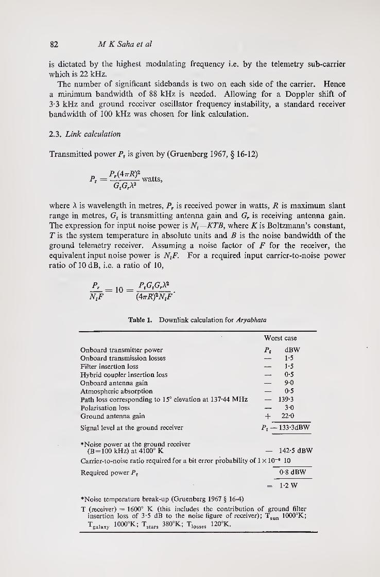
82 M K Saha et al
is dictated by the highest modulating frequency i.e. by the telemetry sub-carrier which is 22 kHz.
The number of significant sidebands is two on each side of the carrier. Hence a minimum bandwidth of 88 kHz is needed. Allowing for a Doppler shift of 3-3 kHz and ground receiver oscillator frequency instability, a standard receiver bandwidth of 100 kHz was chosen for link calculation.
2.3. Link calculation
Transmitted power Pt is given by (Gruenberg 1967, § 16-12)
Pr(4nRf
GtGr A2 watts.
where A is wavelength in metres, Pr is received power in watts, R is maximum slant range in metres, Gt is transmitting antenna gain and Gr is receiving antenna gain. The expression for input noise power is Ni=KTB, where K is Boltzmann’s constant, T is the system temperature in absolute units and B is the noise bandwidth of the ground telemetry receiver. Assuming a noise factor of F for the receiver, the equivalent input noise power is NtF. For a required input carrier-to-noise power ratio of 10 dB, i.e. a ratio of 10,
F. _ ,ft _ P, O.C,A»
N,F (4ir RfN,F
Table 1. Downlink calculation for Aryabhata
Onboard transmitter power
Worst case
Pt dBW Onboard transmission losses — 1-5 Filter insertion loss — 1-5 Hybrid coupler insertion loss — 0-5 Onboard antenna gain — 9-0 Atmospheric absorption — 0-5 Path loss corresponding to 15° elevation at 137-44 MHz — 139-3
Polarisation loss — 3-0 Ground antenna gain 4- 22-0
Signal level at the ground receiver Pt — 133-3dBW
♦Noise power at the ground receiver (B=100 kHz) at 4100° K — 142-5 dBW
Carrier-to-noise ratio required for a bit error probability of 1 X 10⁻⁶ 10
Required power Pt 0-8 dBW
♦Noise temperature break-up (Gruenberg 1967 § 16-4)
= 1-2 W
T (receiver) = 1600° K (this includes the contribution of ground filter insertion loss of 3-5 dB to the noise figure of receiver); Tsun 1000°K;
Tga.axy 1000°K; Tstars 380°K; T]osses 120°K.

The communication system 83
Table 2. Transmitter specification
1. Transmitter power 1-2 W minimum across 50 ohms
2. Operating temperature range — 10°C to 60°C
3. Transmission bandwidth 100 kHz
4. Phase modulation index 1 radian
5. Modulation frequency less than 30 kHz
6. D.C. power less than 4 W at 14 V.
3 o a 5*
T> C
osc \J7-18mHz
buffer
phase modulator
doubler
1 doubler
2
power amp
68* 72 mHz
1
varactor doubler
powc 137.4
»r amp 4 mH*
Figure 3. Block schematic diagram of the onboard transmitter
From this we arrive at the required transmitted power Pt. Table 1 shows the down¬ link break-up and table 2, the transmitter specifications.
The required transmitter power of 1-2 W was realised by an eight-stage network shown in block schematic diagram in figure 3. The first stage was a temperature compensated crystal oscillator at 17-18 MHz buffered by a second stage transistor. The output of the buffer was fed to a constant amplitude variable phase filter of characteristic impedance of 100 ohms. Also fed to this stage were the modulating frequencies which vary the phase of the carrier at the modulation rate, the maximum phase change being 1 /8 radian. The output of the modulator was doubled by two stages of transistor amplifiers. Output of the second doubler fed a low power amplifier whose output was 150 mW at 68-72 MHz. This was further multiplied by a varactor doubler to provide a carrier power of 70 mW at 137-44 MHz, to the final stage power amplifier. The combination of varactor and transistor

84 M K Saha et al
doublers provided a d.c. to a.c. conversion efficiency greater than 30%. Radio frequency power of 1-2 W was fed to a filter, to reject wideband noise in the telecommand band. Output of this filter was fed through a command-operated coaxial relay, which selected either transmitter-1 or transmitter-2, to hybrid coupler on its onward path to antenna.
2.4. Hybrid coupler
To use the same set of antenna for both onboard telecommand reception and tele¬ metry transmission, the hybrid coupler was required. The hybrid coupler connects the transmitter, receiver and antennae together with proper matching between them, at the same time isolating the sensitive receiver from the telemetry transmitter.
2.5. Evolution of design
A hybrid coupler is a four-port device which is ideally loss-less. The scattering matrix of such a device is a unitary matrix. The scattering matrix of a general four-port device is (Collin 1966, p. 174)
Sn S12 *-*13
Sn S22 *-*23 *-*24
*-*31 S32 *-*33 *-*34 5
Sa *-*42 “-*43 *^44 J where Smn = bjan, b,„ is the power leaving the port m and an is the power incident on the port n. The other condition is that in the coupler all ports are to be matched perfectly and opposite ports are to be isolated completely. Imposing this, the above matrix is reduced to
0 S±2 0 5%
_ *$21 0 S23 0 0 S32 0 su •
_ *$41 0 *-*43 0 _
The power dissipated in the coupler should be zero, so imposing the conditions of a unitary matrix, the above matrix is reduced to
“0 (i)i 0 (*)*“
(IJ* 0 (# 0 0 (*)* 0 -(*)* •
_(*)* 0 -(*)* 0
The above mathematical model of the hybrid coupler can be realised with reasonable approximation using practical circuit elements as shown in figure 4.
Imposing the above conditions, S3i=Si3= —(£)* implies that between ports 3 and 4 there is a phase shift of 180° more than between any other adjacent ports. The equalities S12= ($)l=S14i etc., indicate that power flowing into any port is equally divided between the two adjacent ports.
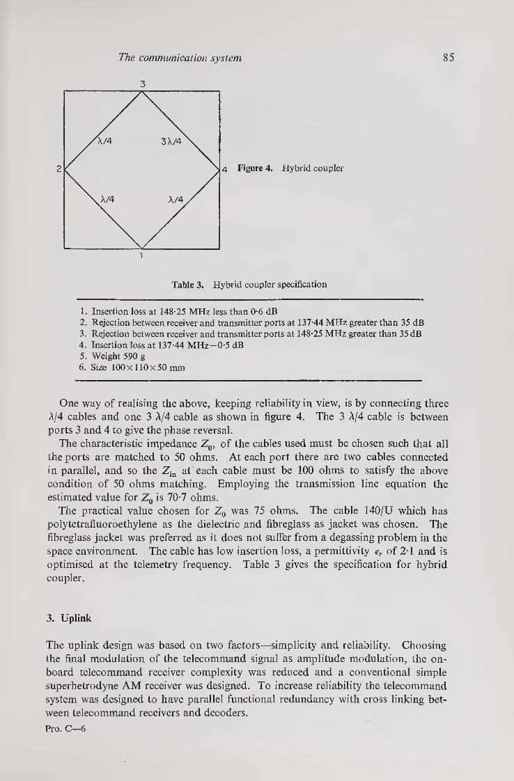
The communication system 85
Table 3. Hybrid coupler specification
1. Insertion loss at 148-25 MHz less than 0-6 dB 2. Rejection between receiver and transmitter ports at 137-44 MHz greater than 35 dB 3. Rejection between receiver and transmitter ports at 148-25 MHz greater than 35 dB 4. Insertion loss at 137-44 MHz—0-5 dB 5. Weight 590 g 6. Size 100 x110 x50 mm
One way of realising the above, keeping reliability in view, is by connecting three A/4 cables and one 3 A/4 cable as shown in figure 4. The 3 A/4 cable is between ports 3 and 4 to give the phase reversal.
The characteristic impedance Z0, of the cables used must be chosen such that all the ports are matched to 50 ohms. At each port there are two cables connected in parallel, and so the Zin at each cable must be 100 ohms to satisfy the above condition of 50 ohms matching. Employing the transmission line equation the estimated value for Z0 is 70-7 ohms.
The practical value chosen for Z0 was 75 ohms. The cable 140/U which has polytetrafluoroethylene as the dielectric and fibreglass as jacket was chosen. The fibreglass jacket was preferred as it does not suffer from a degassing problem in the space environment. The cable has low insertion loss, a permittivity er of 2-1 and is optimised at the telemetry frequency. Table 3 gives the specification for hybrid coupler.
3. Uplink
The uplink design was based on two factors—simplicity and reliability. Choosing the final modulation of the telecommand signal as amplitude modulation, the on¬ board telecommand receiver complexity was reduced and a conventional simple superhetrodyne AM receiver was designed. To increase reliability the telecommand system was designed to have parallel functional redundancy with cross linking bet¬ ween telecommand receivers and decoders.
Pro. C—6

86 M K Saha et al
3.1. Receiver uplink filter
This was a pass band filter with a centre frequency of 148-25 MHz and with an inser¬ tion loss of 3-5 dB Saturation level of front end amplifier was —46 dBm. Assuming a safety margin of 10 dB, the rejection required at 137-44 MHz, was greater than 50 dB. This was realised by four anti-resonant circuits, a combination of two series and four parallel LC network, the series port acting as a trap and the parallel port acting as a passband filter.
3.2. Receiver
Development of 1 kW ground transmitter was assumed to be feasible and on that basis system parameters were estimated and the receiver sensitivity requirement was found to be —96 dBm. The total gain requirement of the receiver was 116 dB to provide an output of at least 2 V peak-to-peak signal with an output signal-to-noise ratio of at least 13 dB for proper decoding of the commands. Table 4 gives the uplink break-up.
The receiver was a single superheterodyne type designed with a low noise preampli¬ fier (noise figure=2-5 dB, gain=16 dB), a local oscillator at 137-55 MHz, a transistor mixer, a three-stage IF amplifier at 10-7 MHz providing a gain of 64 dB, an envelope detector and two stages of audio amplifiers with a total gain of 30 dB. The bandwidth of 30 kHz, required to accommodate the modulating signal of 6-25 kHz, the Doppler shift of ±3-5 kHz and frequency drifts of onboard local oscillator and ground transmitter (0 002%), was provided by a crystal filter at the IF stage.
The block schematic diagram of the receiver is given in figure 5.
4. Brief fabrication details
The telemetry transmitters and the telecommand receiver were fabricated using fibreglass printed circuit boards. The screened electronic components used in
Table 4. Uplink calculation for Aryabhata
Ground transmitter power Ground station losses Ground antenna gain
Worst case +30 dBW -4-5 dB + 16
Path loss corresponding to 10° elevation at 148-25 MHz —141 Atmospheric attenuation Polarisation loss Onboard antenna gain Hybrid coupler loss Power split Filter insertion loss
-0-5 -3.0 -9.0 -0-5 -3-0 -3-5
-119 dBW -126 dBW
Power level at the input of onboard receiver Receiver sensitivity
Margin 7 dB

The communication system 87
Figure 5. Block diagram of the command receiver.
the units were derated to withstand temperature extremes of —15°C to 60°C. The components were mounted close to the board and were potted. The fabricated printed circuit boards were then housed in a milled aluminium box of 2 to 4 mm thickness to prevent high frequency radiation. The mounting holes of these boards with the aluminium chassis were carefully chosen to suppress severe mecha¬ nical vibration. The assembled units were then subjected to shock, vibration, thermal cycling and live test in a thermovacuum chamber to the required flight qualification level.
5. In-orbit performance of the communication subsystem
Prior to launch, the onboard communication system compatibility with ground stations at Bears Lake, USSR and SHAR, India, was tested with the help of a heli¬ copter. The results were positive and the test methods used were later adopted to evaluate the in-orbit performance of the communication system.
5.1. Downlink
Important parameters of interest were (a) link compatibility with theoretical estimate, (b) modulation index variation, and (c) carrier frequency. Link com¬ patibility was determined from ground station receiver data supplied by the Bears Lake Station and SHAR. A histogram of the signal strength is shown in figure 6, the average was estimated to be —133 dBW. This corresponds to a carrier-to-noise ratio of 10 dB for an antenna look angle of 15°. The signal received was of good quality confirming the theoretical estimate.
The received spectrum observed showed a carrier spectrum accompanied by two sideband spectra on both the sides of the carrier. The ratio of carrier-to-first sideband was 1-5 against the theoretical value of 1-7. Hence, the deviation was 2 kHz above the rated value. However, this was within the tolerance. The carrier frequency stability was not determined with sufficient accuracy.
5.2. Uplink
The important parameter of interest was link compatibility with theoretical estimate.

88 M K Saha et al
This was evaluated from onboard receiver automatic gain control data telemetered
to ground. Observations showed the matching of theoretical estimate for an antenna
look angle of 15°.
6. Conclusions
The communication system of Aryabhata has been functioning satisfactorily. The
duration of reception of the signal was in accordance with calculations. Theoretical
link estimates matched well. Onboard transmitter receiver combination worked well
in the transponder mode.
Acknowledgements
The authors acknowledge Prof. U R Rao for his encouragement, Mr L S
Satyamurthy for coordination, and Messrs M R Deshpande and M Ratnakumar for
fabrication of the onboard communication system.
References
Brown J and Glazier E VD 1964 Signal analysis (New York: Reinhold Pub. Corpn.) Collin R E 1966 Foundations for microwave engineering (Tokyo: Kogakusha Book Co.) Gruenberg E L 1967 Handbook of telemetry and remote control (New York: McGraw Hill) ITT 1972 International Telephone & Telegraph Company Reference 'data for radio engineers
(New York: Howard W. Sams)

The telecommand system
R ASHIYA, J P GUPTA, Y K SINGAL, D VENKATARAMANA, A BHASKARANARAYANA, U N DAS and B V SESHADRI ISRO Satellite Centre, Peenya, Bangalore 560 058
MS received 28 April 1977; revised 25 December 1977
Abstract. The telecommand system plays an important role in the success of any satellite mission. This paper provides insights into the design, development and evolu¬ tion of the Aryabhata telecommand system. The paper includes detailed specifications and performance of both the ground and onboard segments of the telecommand system.
Keywords. Command systems; coding; satellite telecommand.
1. Introduction
For effective control of different performance modes of the various satellite sub¬ systems under all conditions, a highly efficient and responsive telecommand (TC) system is absolutely essential. Some of the important operations performed by the telecommand system include energising various subsystems, tape recorder operations, spin-up of satellite, phased operation of experiments, and switching over to redundant system during emergency/failure of main units. Since remote control through telecommand system is the mainstay for these operations to be reliably performed in the satellite in orbit, the system has to work with a high degree of reliability design-wise as well as hardware-wise.
This paper describes the system design, specifications and performance of both the ground and onboard segments of the telecommand system developed for the space¬ craft Aryabhata.
2. Design objectives
The command system was designed to meet the following design requirements; (i) high rejection of spurious signals, (ii) minimum power consumption,
(iii) maximum reliability.
2.1. High rejection of spurious signals
To meet the requirement of high rejection of spurious signals, a coding scheme of 6-bit codes, where codes were limited to combinations of 3 Ones and 3 Zeros was selected. This code was designed to provide maximum protection against spurious triggering of command decoding circuitry while using a relatively narrow
89

90 R Ashiya et al
bandwidth. This scheme provided 20 different command codes. This type of code had the property of rejecting all odd errors and 42% of even errors.
Originally the command frame consisted of a command word repeated 5 times. Due to the occurrence of spurious commands during tests the scheme of command comparison was incorporated. In this scheme, the onboard decoder had a memory and a bit by bit comparison facility. Command decoding was enabled only if two received commands were found to be identical bit by bit. With the introduction of the command comparison scheme the occurrence of spurious commands was elimi¬ nated.
As command codes consisting of 3 Ones and 3 Zeros were being used by other spacecraft, to prevent unwarranted execution of commands meant for some other satellite, an address was introduced. The address code word had a ‘Hamming distance’ of 3 with respect to any command code word. The decoding scheme was modified so that command comparison circuitry could work only after reception of a proper address code and the decoding circuitry was enabled only after reception of two identical command code words. To include the address, the command frame was restructured to a frame of two address words followed by four command code words.
2.2. Minimum power consumption
The onboard command system circuitry had extensively relied upon the use of com¬ plementary symmetry metal oxide semiconductor devices commonly known as COS/MOS. The COS/MOS devices offered the ultimate choice for low static power dissipation and extremely high noise immunity. These devices had the property of increasing dynamic power dissipation with the frequency of operation. However, dynamic power dissipation of COS/MOS was less than any other digital IC family for frequencies below 5 MHz. As dynamic power dissipation depended upon the capacitance and frequency product, care was taken to maximise values of resistors and minimise the values of capacitors, the efforts were limited only by the reliability considerations. The input biasing resistors also added up to extra power consumption and the values of these resistors were maximised to 1 megaohm to reduce this type of power drain. The biasing resistor could not be increased further without increasing the unreliability. By extensive use of medium scale integration (MSI) functions, the number of biasing resistors was reduced to the minimum, resulting in further reduction of dynamic power consumption. For switching functions, the use of latching relays was maximised. The non-latching relays were used only if functional and reliability considerations made such use in¬ dispensable.
These considerations resulted in a system design where both the static and dynamic power dissipation had been minimised without sacrificing reliability. The static power dissipation for the complete onboard command system had a negligible figure of 25 mW.
2.3. Maximum reliability
The onboard command system was designed and fabricated to provide maximum reliability. Selective use of redundancy was made to achieve maximum reliability

The telecommand system 91
keeping extra circuitry to a minimum. Two subcarrier demodulators and two decod¬
ing sections were operating independently and in parallel. Cross coupling between
the subsarrier demodulators and decoding sections increased the reliability since
either subcarrier demodulator and either decoding section can fail simultaneously
without affecting the command operation. Though full redundancy was adopted for
the subcarrier demodulator and decoding section, only necessary line redundancy
and duplication of circuitry for critical and vital functions were incorporated for
command control units and energising unit.
The complete onboard system was arranged into six boxes, i.e., two decoders, three
command control units and an energising unit. Both decoders were identical func¬
tionally, electrically and mechanically. Each decoder incorporated one subcarrier
demodulator and one decoding section. The circuitry between command control
units was partitioned in such a way as to minimise the interface between the different
boxes resulting in a minimum number of interconnecting wires and increased reliabi¬
lity.
All the units were housed in milled aluminium boxes which provided rigid mecha¬
nical support, radiation and RF shielding for the electronics. Input/output points
of each unit were separated out functionally into logic inputs, power supply inputs,
interconnections, telemetering points, ground checkout and testing points and output
lines and were terminated on separate connectors. Such functional separation of
wires reduced the risk of any failure due to wiring harness. Independent testing of
each box and step by step integration of boxes into the complete command system
were made possible.
To match the power distribution with the redundancy of the decoders the tele¬
command system was fed through two failsafe units, one failsafe for each decoder.
As the energising unit and the command control units should work even when one
decoder fails the power outputs of both the failsafes were fed to the command control
units and power switch-on unit through a power ‘Or’ gate.
Each failsafe was designed to supply current to one decoder and to all command
control units and power switch-on unit. This scheme afforded protection against a
short circuit in a decoder power line. However the command control unit power
supply voltage was less than decoder supply voltages, by 600 mV. Diodes in series-
parallel combination were introduced in the decoder supply line to guard the power
supply line against diode failures.
Power supply harness and power distribution scheme were fully redundant. Each
box was powered through two different connector pins and through two different
paths. This ensured that breaking of one supply wire or a bad contact in power
connector would not deprive any box of d.c. power supply.
The d.c. decoupling at the input ‘Or’ gates of command control units guarded
against improper operation of command control units due to output failure of
decoder in any one logic state. Resistive biasing of COS/MOS inputs, which were
likely to float during fabrication, assembly or testing had removed any chance of
COS/MOS failure during these stages due to incidence of stray charges.
3. System specifications
The technical specifications of the telecommand system are presented in table 1.

92 R Ashiya et al
Table 1. Specifications of the telecommand system
Modulation
Carrier frequency
Carrier frequency stability
Carrier modulation
Transmitter output power
Ground antenna gain
Subcarrier frequency
Subcarrier frequency stability
Subcarrier modulation
Command frame length
Word length
Bit period
Bit rate
Command frame structure
Address code
Command execute code
Sync
One
Zero
Blank
No. of command execute codes
No. of direct commands
No. of shared commands
Total number of commands
Signal level at decoder input
Minimum S/NR ratio at the decoder input
PD M/AM/AM
148-25 MHz
±0-002%
75%
1 kW
15 dB
6-25 kHz
±0-002%
100%
48 bits (6 words)
8 bits (sync. 6 code bits, blank)
72 cycles of 6-25 kHz subcarrier (11-52 m/s)
87 bits/s
Two address words followed by four command execute words
111111 (six Ones)
3 Ones and 3 Zeros
54 cycles of subcarrier ‘on’
36 cycles of subcarrier ‘on’
18 cycles of subcarrier ‘on’
Subcarrier ‘ off’ for one bit period
20
5
30
35
2 V to 7 V peak to peak
13 db
4. System implementation
The onboard telecommand chain consists of a turnstile antenna, hybrid coupler, power divider, command receiver, command decoder and command control units. The antenna, hybrid coupler, power divider and command receivers are described elsewhere. The command decoder and the command control units will be described here. There are two identical decoders and four control units for command execu¬ tions. Figure 1 shows the onboard command system block diagram.
The incoming signal is received by the antenna. The hybrid coupler isolates the outgoing telemetry signal from the incoming command signal. The output of the hybrid coupler is fed to the power divider which feeds the received command signal to the two receivers in equal proportions. The receiver detects and demodulates the received signal and makes the modulated subcarrier signal available as output.
The incoming signal from the receiver is fed to two active 2-pole bandpass filters (BPF) each having a centre frequency of 6-25 kHz and ± 7-5 % bandwidth.

The telecommand system 93
snap signal (separation)
Figure 1. Onboard command system block diagram
This filter improves the S/N ratio by 16 dB. The BPF output is fed to the ampli¬ fier. The amplifier chosen has a voltage gain of 8.
The amplifier output is sliced at about 50% level to eliminate the base line noise. The high noise immunity property of COS/MOS devices is used for this purpose. The sliced output is shaped by two inverters to maintain the correct polarity. The output of the shaper consists of pulses at subcarrier frequency.
The shaper output is given to the cross-coupling network. It is a passive RC net¬ work where outputs from its preceding chains are given to two succeeding chains so that even if there is a failure in one of the preceding chains and another failure in any of the succeeding chains the link still works. As the passive RC network is used for the purpose of cross coupling, d.c. coupling between the preceding and succeeding chains is avoided to prevent failure mode effect on the succeeding chains.
The outputs of the cross-coupling network are fed to the two decoders. The out¬ puts from both the decoders are given to the respective command control units for the command execution. The energising unit switches the raw power (solar/chemical battery) to the onboard regulators on receipt of the rocket signal or in case of rocket signal failure, the snap signal. The decoder and the command control units are discussed in more detail in the following sections.
4.1. Decoder
A block diagram of the decoder is shown in figure 2. The shaper output is fed to the clock pulse generator and the subcarrier demodulator through the cross-coupling network. This demodulator consists of COS/MOS gates and capacitor charging¬ discharging is used to strip out pulse duration modulation (PDM) waveform from subcarrier modulated signal. This gives the original PDM waveform, and at the same time the number of subcarrier pulses in each burst is counted by the ‘ bit

94 R Ashiya et al
to command control units
Figure 2. Decoder block diagram
separator ’ to separate out Zero, One and Sync. Zero, One and Sync thus separated are made available on three different lines.
A Sync has to be obtained first before starting further processing. The Sync pulse thus separated is also used to trigger the ‘ frame timing generator ’ which provides time slots for each of the word periods within a frame.
The number of Ones is counted in the ‘ code format check section ’. The correct address word must contain 6 Ones. The address recognition section, upon reception of a correct address word enables a gate to generate the execute pulse.
The clock pulses for the shift register are derived from the trailing edges of the PDM bits. No clock pulse is generated if the PDM bit contains less than 9 sub¬ carrier pulses. This minimises the effect of spurious spikes.
The first two address words are followed by four execute words. The first execute word is shifted into the six-stage main register. Only Ones are shifted into the regis¬ ter. The second execute word is shifted into the auxiliary register through selective steering circuit, while the contents of the main shift register are recirculated.
In both the registers, the serial information being recirculated is also fed into the command comparison logic where both the words are compared bit by bit. The third execute word is steered directly into the command comparison logic and is not stored anywhere. The third execute word is compared bit by bit with the first execute word stored in the main register and also with the second execute word stored in the auxiliary register. A ‘ coincidence pulse ’ is generated on reception of any two iden¬ tical execute words, by the command comparison logic (CCL) and it is fed to the execute pulse generator (EPG). In the case of execute words 1 and 2 being identical, the command stored in the main register is treated as valid command.

The telecommand system 95
In the case of execute words 1 and 3 being identical, the desired command is in the main register. If, however, execute words 2 and 3 are identical, a ‘ transfer pulse ’ is generated which transfers the contents of the auxiliary register in parallel to the main register. This way the valid command is always available in the main register. Hence the decoding matrix is connected to the main register only.
An execute pulse is generated by the EPG upon reception of a coincidence pulse from CCL but only if enabling signals from the address recognition and code format check sections are present. The execute pulse enables the decoding matrix to decode the code. The output of the decoding matrix is available on 20 different lines, each corresponding to the particular execute code transmitted.
Output pulses of code nos. 3, 4 and 5 are used as direct commands. Pulses of code 1 and 2 are used as mode-A and mode-B commands in the mode generator to generate the mode-A and mode-B control signals for the 30-command generator.
The 30-command generator is a bank of 15 SPDT solid state switches. Depending upon the mode-A, mode-B control status, the pulses corresponding to any code from code 6 to code 20 can be routed to either of the lines. This way 15 codes are made to generate 30 commands. The 30 mode-controlled commands and the 3 direct commands are then fed to the command control units.
Table 2. Command allocation chart
SI. No.
Command No.
Command Designation
Command function/operation
1. 1 Mode-A Switches command decoding circuits to mode-A
2. 2 Mode-B Switches command decoding circuits to mode-B
3. 3 Storage TM (a) Switches the tape recorders to playback mode. (b) Switches telemetry to storage mode (c) Starts a timer which after 5 min switches
telemetry to real time mode
4. 4 Real time TM Switches telemetry to real time mode
5. 5 TR record (a) Switches the tape recorders to record mode (b) Switches telemetry to real time mode
6. 6A TR input Off Disconnects the telemetry encoder output from tape recorder input
7. 7A TR input On Connects output of telemetry encoder to input of tape recorder
8. 8A Encoder-2 Selects PCM and PCM complement signals from telemetry encoder No. 2
9. 9A Encoder-1 Selects PCM and PCM complement signals from telemetry encoder No. 1
10. 10A SCO-2 Connects output of subcarrier oscillator No. 2 from telemetry to input of telemetry transmitters
11. 11A SCO-1 Connects output of subcarrier oscillator No. 1 from telemetry to input of telemetry transmitters.
12. 12A Expts. Off Switches Off d.c. power supply to Expt. 1, Expt. 2 and Expt. 3
13. 13A Expt. 1 On Switches On d.c. power supplies to Expt. 1 14. 14A Expt. 2 On Switches On d.c. power supplies to Expt. 2
15. 15A Expt. 3 On Switches On d.c. power supplies to Expt. 3

96 R Ashiya et al
Table 2. Command allocation chart (Contd.)
SI. No.
Command No.
Command Designation Command function/operation
16. 17A TR2 On Connects the power and control circuits to tape recorder No. 2 and disconnects the same from tape recorder No. 1
17. 18A TR 1 On Connects the power and control circuits to tape recorder No. 1 and disconnects the same from tape recorder No. 2
18. 16A TR’s Off Stops the tape recorder from recording or playing back if tape recorder has been in record or playback mode
19. 19A TC test-2 Switches the TC test relay pole to 0 V on application of this command
20. 20A TC test-1 Switches the TC test relay pole to + 9 V on appli¬ cation of this command
21. 6B SS override Removes inhibit signal for spin commands which is generated by sun sensor when spin rate of satellite is more than 20 rev/min
22. 7B Spin arm Makes spin circuits ready for receiving the spin command
23. 8B Spin-3 Fires spin bottle No. 3
24. 9B Spin-4 Fires spin bottle No. 4
25. 10B Spin-5 Fires spin bottle No. 5
26. 11B Spin-6 Fires spin bottle No. 6
27. 12B Tx-2 On (a) Switches On d.c. power supply to telemetry transmitter No. 2
(b) Switches Off d.c. power supply to telemetry transmitter No. 2
(c) Connects output of telemetry transmitter No. 2 to input of hybrid coupler
28. 13B Tx-1 On (a) Switches On d.c. power supply to telemetry transmitter No. 1
(b) Switches Off d.c. power supply to telemetry transmitter No. 2
29. 14B PHA-2 On Switches On pulse height analyser No. 2 for Expt. 1 and switches Off pulse height analyser No. 1
30. 15B PHA-1 On Switches On pulse height analyser No. 1 for Expt. No. 1 and switches Off pulse height analyser
No. 2
31. 16B Reserve Spare command
32. 17B PCM comple¬ ment
Selects PCM complment data from tape recorder output channel No. 2 during TR playback for trans¬ mission of telemetry data.
33. 18B PCM Selects PCM data from tape recorder output chan¬ nel No. 1 during TR playback for transmission of telemetry data
34. 19B Tracking On Connects tracking output from command receivers to input of telemetry transmitters
35. 20B Tracking Off Disconnects tracking output of command receivers from input of telemetry transmitter.

25
6 B
PS
The telecommand system 97
o C
L. Q> l_
0)
L- <D
* * O o o Q. a a
Fig
ure
3.
Onboar
d c
om
man
d o
per
atio
ns

98 R Ashiya et al
4.2. Command control units
The command control units execute the various commands. Table 2 gives the func¬
tions performed by the different commands and figure 3 shows the onboard command
operations in a schematic way. The execution of different commands is allocated
to these command control units.
4.2a. Command control unit-\
This unit executes the commands corresponding to the experiments and telemetry
transmitters. On command, this unit switches On/Off the d.c. power supply inputs
of the telemetry transmitter and also selects the r.f. output of the on-telemetry-
transmitter for connection to the antenna through the hybrid coupler. On receipt
of commands for the experiments, this unit switches On/Olf d.c. power supply inputs
of the respective experiment. This unit also provides the control signal for switching
On/Off the pulse height analyser of the x-ray astronomy experiment.
4.2b. Command control unit-2
This unit executes the commands controlling the tape recorder (TR) and telemetry
operations.
The storage telemetry and real time telemetry commands operate a solid state
(COS/MOS) DPDT switch to select the direct data from telemetry or the played back
data from the tape recorder to the transmitters through the sub-carrier oscillators
(SCO). In addition, the storage telemetry command also puts the tape recorder
into playback mode. The storage telemetry command also triggers the two onboard
timers which, in turn, generate real time telemetry command after 5 min.
The TR record command puts the tape recorder into record mode. This command
also operates the COS/MOS SPDT switch to connect the direct data from telemetry
to transmitter through the subcarrier oscillators.
The TR 1 ‘ On ’ command connects the power and control circuits to tape recorder
No. 1. The TR 2 ‘ On ’ command connects the power and control circuits to the tape
recorder No.2. TR’s Off command stops the tape recorder from recording if the tape recorder
is in the record mode or from playing back if it is in playback mode.
The PCM and PCM complement commands operate a solid state (COS/MOS)
DPDT switch to select the PCM data or PCM complement data for transmission
during storage telemetry mode. The SCO-1 and SCO-2 commands operate On and Off coils of a latching relay
to select the output of SCO-1 or SCO-2 for connecting to the transmitters input for
transmission of telemetry data. The TC test-1 and TC test-2 commands operate On and Off coils of a latching
relay to connect the TC test monitoring line to +9/OV.
4.2c. Command control unit-3 and power switch on unit
These two units work in conjunction to control the spin-up system and tracking

The telecommand system 99
Figure 4. Telecommand ground station
system. These units are used for energising all satellite subsystems by the rocket
signal. In case of a failure of the rocket signal, this unit energises the satellite by the
signal generated at the time of the separation of the satellite from the rocket. With
the help of the timers which are activated by the satellite power switch On, this unit
fires the first spin bottle after 27 s and the second spin bottle after 89 s of the
power switch On, to impart an initial spin rate of 90 rev/min to the satellite. The
remaining four spin bottles are fired by this unit on reception of the proper spin
command preceded by the Spin Arm Command. This unit also connects and dis¬
connects the tracking signal to the telemetry transmitters.
This unit also incorporated the required circuitry to disconnect the spin-up system
during ground checkout of the satellite at the launch pad.
5. Ground command system
The ground telecommand chain consists of a command encoder, a command trans¬
mitter and a command antenna. Figure 4 shows a block diagram of the telecom¬
mand ground station set-up. The command encoder and the transmitter are
described in detail separately. The command code output of the command encoder
is connected to a digital printer, which records the comm.and sent and the time of
transmission of the command. The command frame output of the command
encoder is connected to the r.f. transmitter and the output of the transmitter is
connected to the command antenna. To increase the reliability of the ground
station, two encoders and two transmitters are provided at each station.
5.1. Encoder
The command encoder generates 20 different command frames corresponding to 20
different command execute codes. With the help of the front-panel-mounted
100 R Ashiya et al
command selector switches any one of the twenty execute codes can be selected at a
time. The command frame amplitude modulates the 6-25 kHz subcarrier to a depth
of 100%.
A crystal-controlled master oscillator generates a 100 kHz master clock. This
master clock is fed to a 4-stage binary divider which generates 6-25 kHz clock. The
6-25 kHz clock is fed to the subcarrier generator and timing waveform generator.
The subcarrier generator is an active band pass filter with a centre frequency of 6-25
kHz. The output of this subcarrier generator is a 6-25 kHz sine wave.
These output pulses of 6-25 kHz are again divided in timing waveform generator
by 18 to produce necessary basic timing signals which are again processed through
two-stage binary counter to generate sync, one and zero pulses continuously on the
three separate lines. These Sync, Ones and Zeros are combined in the proper order
to generate the command frame. This command frame consists of two address
words followed by four execute words.
This command frame is used as a control voltage of an analog switch for switching
6-25 kHz sine wave subcarrier to obtain PDM/AM signal at 100% modulation and is
fed to VHF transmitter for transmission. Any desired command can be manually
set with address in the command console and transmitted with a single depression of
the ‘ GO ’ switch provided in the console. Seven banks of 5 key piano switches are
provided to select any one of the 35 commands. The code is first converted into a
decimal form and then it is displayed on the front panel. Subcarrier level indicator
and mode indicator are provided in the console along with the supply voltage and
current indicators. The complete code can be printed along with the time of sending
using any digital printer and the necessary interface required is housed in the
console.
6. Link calculation
The output power of the command transmitter is fixed at 1 kW. The ground
station cabling distance from the command transmitter to the command antenna
is about 15 m. The cabling and other ground station losses are assumed to
be about 2-5 dB and the ground telecommand antenna gain is about 15 dB.
Since the range is constantly changing in the satellite system, the path loss is variable.
For Aryabhata which is in a near circular orbit of 600 km, the minimum distance
between the antenna and the satellite is 600 km and the maximum distance is 2800 km
for zero degree elevation of the satellite. So, if the command has to be attempted at
near zero degree elevation, the transmitter must have sufficient power for a range of
2800 km. The satellite antenna pattern has a dip of about 9 dB in certain directions.
This aspect has also been taken into consideration in determining the transmitter
power. The complete link calculation of the command chain, taking into account
these considerations is given in table 3.
7. Command transmitter
The command transmitter is an AM transmitter which delivers an output power of
1 kW at the carrier frequency of 148-25 MHz. The transmitter can be modulated to

The telecommand system 101
Table 3. Uplink estimation
Item Gain/loss Net power
in dBs dB
1. Transmitter power
2. Ground station loss (due to cables connectors
Pt
rotary joint and polarisation switch) -2-5
3. Ground antenna gain 15
4. E. radiated power Pt +12-5
5. Tracking loss -0-3
6. Maximum propagation loss -145
7. Atmospheric attenuation -0-5
8. Fading margin -5
9. Polarisation -3
10. Power available at satellite antenna R, —141-3
11. Onboard antenna gain -9 12. Hybrid loss 0-5
13. Onboard connector and cable loss -1-2
14. Power split loss -3-0
15. Filter loss -1-0
16. Net power at Rx input A-156 Assumed receiver sensitivity = —126 dBw
So, Pt — 156 dBw = —126 dBw Or, Pt = 30 dBw = 1 kW
Receiver front end noise power = 148-5 dBw (assuming I.F. bandwidth
of ±15 kHz,) Input to the receiver = —126 dBw Input S/N of the receiver = 22-5 dB This S/N at the input of the receiver is sufficient to produce sufficiently good output
S/N.
a depth of 80% without excessive distortion and the modulation frequency can be between 300 Hz and 10 kHz. The transmitter is essentially a class C plate modulated r.f. amplifier and uses a forced air cooled power stage. The carrier is generated at half the traffic frequency which is 74T25 MHz and then it is doubled and amplified to a level of 60 W to drive the final power amplifier.
For convenience of installation, operation and maintenance, the transmitter has been divided into four major blocks: (1) power amplifier; (2) low power unit; (3) modulation amplifier; (4) HV power supply and control circuit.
All these blocks have been fabricated into individual units and have been mounted in a 19 in. rack.
8. Tests and performance evaluation of the command system
The test and evaluation philosophy for the telecommand system incorporates rigorous testing at all levels of fabrication, handling and integration of the onboard tele¬ command system. To enable systematic testing, a Command Test Console was
Pro. (C)—7

102 R Ashiya et at
developed and fabricated. This console was used to test individual command system boxes, the complete integrated onboard command system and the command system during various steps of integration with the spacecraft for all parameters and functional operations.
The test sequence for the onboard system included cold exposure at —30°C for 6 hr, hot exposure at +60°C for 6 hr, cold soak at — 10°C for 6 hr, hot soak at -f 50°C for 6 hr, 5 g vibrations at 30 Hz to 60 Hz for 5 min and 20 shocks each of 20 g acceleration for 10 ms duration. These tests were followed by a thermovac test at -f-503C and 1 X 10~5 torr pressure for 24 hr and at — 10°C and 1 x 10⁻⁵ torr pressure for 24 hr.
8.1. Special tests
In addition to these environmental tests, the telecommand system along with the other systems was subjected to balloon test, helicopter test and aircraft test. The preprototype of the satellite was flown to a height of 35 km on a plastic balloon. Both the uplink and downlink were tested.
The helicopter test has been performed at SHAR with the preprototype and the prototype models of the satellite. This test has been used to qualify the telemetry and telecommand systems of the ground station and it also provided useful data of the simulated working of satellite during flight.
The aircraft test was carried out with the help of the prototype of the satellite at Bears Lake in Moscow for qualification of the telemetry and telecommand system of the Bears Lake ground station. The worst case link conditions were simulated and the actual operation of the satellite was checked under these conditions.
months after launch ,
Figure 5. Histogram of command operations

The telecommand system
Table 4. Summary of command operations till 10 April 1976
103
Command Number
Commands attempted
Commands executed
Commands failed to execute
in one pass
1 149 148 1 2 140 138 2 3 115 112 3 4 3 3 —
5 5 5 -_
6A — — —
7A 1 1 —
8A 2 2 —
9A 3 3 —
10A 1 1 —
11A 1 1 —
12A 27 27 —
13A 10 10 —
14A 8 8 _
15A 7 7 —
16A 9 9 _
17 A 6 6 —
18A 1 1 —
19A 19 18 1 20A 19 18 1 6B 2 2 —
7B 2 2 _
8B 1 1 _
9B — — _
10B — — _
11B — — _
12B 1 1 _
13B 1 1 _
14B 9 9 _
15B 9 9 _
17B 1 1 _
18B 2 2 0 19B 132 129 3 20B 132 129 3
Total 818 804 14
9. In-orbit performance of the telecommand uplink
The telecommand uplink has operated successfully. Regular playback and tone range commands are being exercised from SHAR. Complete control of Aryabhata
through commands has been achieved. The successful execution of more than 800 commands has justified the confidence placed in the command system. Table 4 gives the record of command operations. Figure 5 depicts the performance of com¬ mand operations in a histogram form.
The performance of the uplink has been analysed for the behaviour of the onboard telecommand receiver and for the ability of telecommand decoding system to execute

104 R Ashiya et al
the desired command without errors like failure of command system to effect a desired command and occurrence of spurious and false commands.
It has been observed that occasionally commands operated only after repeated transmission of commands. This phenomenon of the non-operation of the com¬ mands, in spite of the high signal levels can well be due to the highly secured design of the telecommand system. It incorporates a command comparison logic which automatically rejects any command, that has been impaired either by the channel or receiver noise. This logic ensures that only the proper command will be executed and false commands will never be executed. This clearly shows that the comparison logic rejected these commands which must have been impaired by the channel or receiver noise during the respective orbits.
The voice transmission experiment through Aryabhatas as carried out using a 4 kHz carrier frequency modulated by voice frequency of 2 kHz. It is quite probable that the frequency band extended into 6-25 kHz region of the telecommand system and a certain amount of noise is bound to have been injected into the telecommand decoding system. But no spurious operation of command whatsoever has been observed during the voice testing over a number of passes. This confirms the excellent noise immunity of the telecommand decoder.
10. Conclusions
The operation of the command link during the orbital phase has conclusively proved the complete reliability of the Aryabhata command link and command system. The feasibility of the operation of commands even at very low elevation angles of the order of 5° has provided a greater operational manoeuvre over a single pass.
Acknowledgements
Besides the authors who worked on the Aryabhata telecommand system there were many other engineers who actively participated in the design, development and testing of the system. Special mention should be made of Messrs P K Shinde, B B Hakke, N N Singh, R D Bansiya, T S Narayanan, R Lakshminarasimhan and K Sunderesh who have contributed substantially to the content of this paper.

Antenna systems for the ‘ Aryabhata ’ mission
S P KOSTA, S PAL, P K REDDY, V K LAKSHMEESHA, K N S RAO, K N SHAMANNA, V MAHADEVAN, V S RAO and L NICHOLAS ISRO Satellite Centre, Peenya, Bangalore 560 058
MS received 28 April 1977; revised 3 November 1977
Abstract. The onboard and ground antenna system employed in the Aryabhata mission for telemetry and telecommand operations are described. The onboard antenna system common to telemetry and telecommand frequencies consists of four monopoles fed in turnstile configuration and generates a near isotropic pattern with worst dips of the order of —10 dB over approximately 0-2% of the total radiation sphere area. The ground antenna system consists of a high gain (16 dB) telecommand antenna and a telemetry array of eight medium gain Yagis (gain 22 dB).
Keywords. Antennas; electromagnetics; satellites.
1. Introduction
The antenna system employed in the Aryabhata mission for telemetry (TM) and telecommand (TC) operations falls under the following two categories: (1) satellite onboard antenna systems, (2) ground antenna systems.
An onboard antenna system with a near-isotropic pattern both at telemetry (137-44 MHz) and telecommand (148-25 MHz) frequencies was required to meet the communi¬ cation link needs between a ground station and Aryabhata. The requirement for an isotropic pattern was dictated by the fact that the satellite had no attitude control and hence it could take any possible orientation with respect to the ground station during its life in space. A true isotropic pattern is an ideal situation and in practice only approximate isotropy can be realised. The type of approximation is governed by the type of antenna system selected, nature of mount and the size of the body on which the antenna is mounted. The onboard antenna being near-isotropic, to have reliable up-and downlinks, either the respective power of transmitter should be high or the ground station antenna gain should be high. In the case of uplink (telecommand), to some extent, it is possible to have high power transmitter at the ground but the practical constraints to achieve the high power are quite severe and hence a trade-off between the TC transmitter power and the antenna has to be made. The link calculation to account for the worst case onboard condition for maximum slant range showed that a reliable uplink can be established for a ground TC trans¬ mitter power of 1 kW and an antenna gain of 16 dB. For downlink, the onboard transmitter power is very limited, essentially restricted by the available onboard d.c. power. From the link calculations for 600 km circular orbit and for the radiated
105

106 S P Kosta et al
power of 1-5 W by the onboard transmitter, it was found that an antenna of gain 22 dB would suffice for a reliable downlink.
2. Satellite onboard antenna system
The system chosen after considerable study (Brown and Woodward 1947; ESRO- Report 1971; Jasik 1961; Kraus 1950; Pal and Saha 1971; Anon 1967) was that of four quarter wave monopoles made at the mean of telemetry (137-44 MHz) and telecommand (148-25 MHz) frequencies, i.e. 142-85 MHz mounted around the belly band of the satellite and operated in turnstile fashion. The dimensions of the dynamic envelope of the heatshield of the rocket were insufficient to contain the satellite with quarter-wave monopoles mounted perpendicular to the spin axis. This made it necessary to mount the monopoles in an inclined fashion and 45° inclination was chosen as the best value, balancing the inclination and the image effects due to body reflections. The maximum length of the monopoles which could be accom¬ modated was 560 mm (0-257A at 137-44 MHz where A is the wavelength). Any further increase in length, if required, could be achieved by bending the monopoles at the tip parallel to the spin axis to compensate the effect of oblique images of monopoles in the satellite body. Figure la (plate 1) gives the configuration of the monopoles
1 Figure 1 b. Schematic of the antenna feed system

Antenna systems of Aryabhata mission 107
mounted on the belly band of a rhombocubic octahedral satellite with an inclination of 45°.
The feed system using a ring hybrid was designed for : (i) simultaneous handling of telemetry and telecommand signals and (ii) providing a sequential 90° phase shift for four monopoles. The complete feed system is shown in figure lb.
3. Experimental study of the onboard antenna system radiation pattern
Since it is easier to match the impedance than to get the required radiation pattern, an experimental study was undertaken to evaluate the radiation characteristics of the antenna system. Because of the ease of measurement at higher frequencies, the study was made on a 1/3 scale model. The antenna system was made to operate over the frequency band 412-32 and 444-75 MHz (3 times the telemetry and telecommand frequencies respectively). The hybrid coupler was made at 412-32 MHz to give maxi¬ mum isolation between the transmitter and the receiver port at 412-32 MHz. By experimentation the length of each monopole for minimum dip in the gain pattern
O 60 120 180 240 300 360
(j5 (deg)
Figure 2. Onboard antenna gain (dB) characteristics at telemetry frequency (contour plots)

108 S’ P Kosta et al
was found to be 0-257 A (straight)+00274 A (bent) at 412-32 MHz. Since there was more margin at the telecommand frequency, manipulation of the phases of the mono¬ pole excitations was considered without tampering with phase symmetry, for improve¬ ments at 412-32 MHz. Cable harnesses were made at different frequencies to examine the effect of feed phase on the radiation pattern. The cable harness made at 420 MHz (3 X 140 MHz) resulted in a gain pattern with near —10 dB dips at both frequencies.
The radiation pattern measurements were made for vertical and horizontal polarisations at both frequencies covering the entire radiation sphere. A standard dipole was used as a reference. The worst dips observed for vertical and horizontal polarisations were of the order of —20 dBi at both frequencies, where dBi stands for decibels over isotropic level.
The gain patterns are calculated for diversity reception (Pal et al 1976) by combining the results of vertical and horizontal polarisations at each 6 and <£. The results are presented in the form of contour plots in figures 2 and 3, at the telemetry and tele¬ command frequencies, respectively. The overall radiation characteristics were found to accord with expectations. There are four dip zones in the upper hemisphere around
Figure 3. Onboard antenna gain (dB) characteristics at telecommand frequency (contour plots)

Antenna systems of Aryabhata mission 109
0=50° to 60° and an additional four in the lower hemisphere around #=130° to 140° of the omni-radiation sphere. These dip regions are symmetrically placed around the spin axis with an approximate interval of 90°. The null depths are more in the lower hemisphere than in the upper one, which is due to the fact that the antenna system faces more blockage from the lower part of the satellite body than in the upper. Maximum gain is obtained along the spin axis.
Using figures 2 and 3, the percentage of total surface area radiating a certain level is calculated. Such percentage areas for different gain levels at both frequencies are presented in figure 4. From this, the average gains at both frequencies are calculated and these are below the isotropic levels. Efficiencies calculated from these values, which include the feeder mismatch losses and the dissipative losses at the monopoles, are 73% at telemetry frequency and 64% at telecommand frequency.
4. Impedance measurements and final tests
Impedance measurements were carried out on a full scale satellite model. The impe¬ dances at the monopoles were of the order of 50 ohm with voltage standing wave ratio
2 0-2-4 -6 -8 -10 -12
goin (dB) level
Figure 4. Percentage areas at different gain levels

110 S P Kosta et al
less than 2 0 at both frequencies. The voltage standing wave ratio at hybrid ports were found to be less than 1-2 for both frequencies.
Activated solar panels were fixed on the satellite to study the effect of the circulat¬ ing currents on the impedances. The effect was found to be negligible. It was expected that these panels do not have any effect on the radiation pattern either. This was confirmed in actuality.
The final full scale antenna system was qualified after subjecting it to various envi¬ ronmental and mechanical tests according to the following specifications:
temperature range — 10°C to -f-55°C pressure 10~5 torr vibration and acceleration levels 0-2 to 10 g
5. Performance in orbit
After the satellite was placed in orbit, antenna patterns were evaluated from the recordings of automatic gain control (AGC) outputs of two telemetry receivers, and a post-detective type diversity combiner. The two telemetry receivers were connected to two orthogonal linear polarisations. Figure 5 indicates samples of combined patterns, taken at different intervals, in orbit No. 664. The results are
Figure 5. Combined antenna patterns at different intervals of time (T min) during the pass
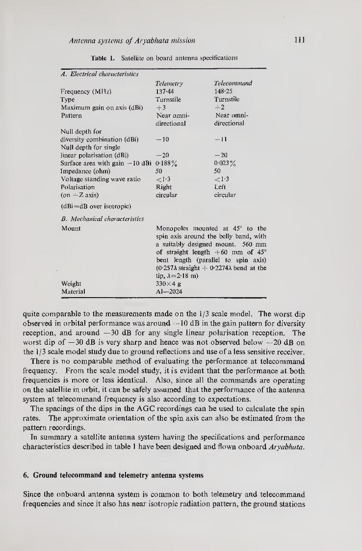
Antenna systems of Aryabhata mission 111
Table 1. Satellite on board antenna specifications
A. Electrical characteristics
Telemetry Telecommand
Frequency (MHz) 137-44 148-25
Type Turnstile Turnstile
Maximum gain on axis (dBi) + 3 +2
Pattern Near omni¬ Near omni¬
Null depth for directional directional
diversity combination (dBi) Null depth for single
-10 -11
linear polarisation (dBi) -20 -20
Surface area with gain —10 dBi 0-188% 0-023%
Impedance (ohm) 50 50
Voltage standing wave ratio <1-3 <1-3 Polarisation Right Left (on + Z axis)
(dBi=dB over isotropic)
circular circular
B. Mechanical characteristics
Mount Monopoles mounted at 45° to
Weight Material
spin axis around the belly band, with a suitably designed mount. 560 mm of straight length +60 mm of 45° bent length (parallel to spin axis) (0-257A straight + 0-2274A bend at the tip, A=2-18 m) 330x4 g Al—2024
quite comparable to the measurements made on the 1/3 scale model. The worst dip observed in orbital performance was around —10 dB in the gain pattern for diversity reception, and around —30 dB for any single linear polarisation reception. The worst dip of —30 dB is very sharp and hence was not observed below —20 dB on the 1/3 scale model study due to ground reflections and use of a less sensitive receiver.
There is no comparable method of evaluating the performance at telecommand frequency. From the scale model study, it is evident that the performance at both frequencies is more or less identical. Also, since all the commands are operating on the satellite in orbit, it can be safely assumed that the performance of the antenna system at telecommand frequency is also according to expectations.
The spacings of the dips in the AGC recordings can be used to calculate the spin rates. The approximate orientation of the spin axis can also be estimated from the pattern recordings.
In summary a satellite antenna system having the specifications and performance characteristics described in table 1 have been designed and flown onboard Aryabhata.
6. Ground telecommand and telemetry antenna systems
Since the onboard antenna system is common to both telemetry and telecommand frequencies and since it also has near isotropic radiation pattern, the ground stations

112 S P Kosta et al
cof^ 5? ^ Ok NioO"J 01 nio — O - OOO'-njc\jc\jc\j ro 066090600O O O ~ 'in oiffl-snomO'j ^ Zl
— n-<\j n 'j 'j in io
1 1 i i I I I I I i I |
<CDUQujiLC)iH^i; O
t
Fig
ure
6.
Tel
ecom
man
d a
nte
nnaj
asse
mbly

Antenna systems of Aryabhata mission 113
antennas have to be of a high gain. From the up- and downlink calculations based on telecommand transmitter power of 1 kW and telemetry transmitter power of 1 -5 W, it was found that a 16 dB telecommand antenna and a 22 dB telemetry antenna would ensure the reliability of operations.
An extensive study was made to achieve these high gain antennas at VHF. It was found from previous studies (Jasik 1961; Wolf 1967; ARRL Handbook) that in VHF range, the Yagi antenna system is best suited considering the electrical and mechanical characteristics of different antenna systems. The required high gain could be achi¬ eved either by a single Yagi antenna or by an array of medium gain Yagi antennas.
In the case of telecommand antenna (required gain 16 dB) a single Yagi was pre¬ ferred over an array to achieve 16 dB gain purely from the point of view of mechanical mounting. It was easy to manoeuver a single Yagi and also it was possible to mount it at the centre of the telemetry antenna array. However, a single Yagi will be very unwieldy for more than 16 dB gain as at axial lengths greater than 4A, the gain in¬ crease is negligible with increase in axial length. Hence, it was decided to have the telemetry antenna of 22 dB gain by arranging medium gain Yagi elements.
7. Telecommand antenna
The telecommand antenna designed was a cross linear polarised antenna. A
Figure 7a. Radiation pattern of telecommand antenna for linear polarisation A and B.

114 S' P Kosta et a/
Table 2. Telecommand antenna specifications
Type
Frequency
Maximum gain
Impedance
Voltage standing wave ratio
Yagi (17 elements, 3-66 A long)
148-25 MHz
16±1 dB over isotropic
50 ohms
<1-25
Pattern (E/H planes)
Beam width
Maximum side lobe level
Back lobe level
Power handling capacity
Band width
Polarisation
Connectors
Physical description
Total length
Maximum width
Material
Weight
: 30°
: -16 dB
: -20 dB
: 2 kW average
: 12 MHz
: Provided with crossed elements resulting in two orthogonal linear polarisation. An external polari¬ sation switch is used to obtain right or left circular polarisations.
: N type (female)
: 7-615 m
: 1-017 m
: Commercial aluminium
: 25 kg
polarisation switch was put at the input of the antenna to achieve left or right hand circular polarisation of the transmitted signal. In the initial phase the antenna element lengths and spacings were adjusted by experimentation to achieve maximum design gain (16 dB) and optimum axial length. Radiation pattern measurements in ground reflection modes were carried out for both the linear polarisation and corres¬ ponding patterns were plotted both for E and //planes. Figure 6 gives the dimensional sketch of the final developed antenna and figure 7a the typical E and H radiation plots for polarisations A and B. Table 2 gives the overall specifications of the telecommand antenna. The results of the measurements indicate that the design is nearly optimum compared to a normal design (Jasik 1961; Wolf 1967; ARRL Hand¬ book) and hence it can be adopted for similar gain requirement conditions after proper scaling. Figure 7b (plate 2) shows the photograph of the telecommand antenna designed and developed at ISAC which is currently being used at Sriharikota Ground Station for sending commands to Aryabhata.
8. Telemetry antenna system
The available telemetry antenna system at Sriharikota, which had servo drive and provision for auto tracking was used after some modifications to suit our require¬ ments. This antenna is an array of eight medium gain (14-7 dB) Yagi elements

Antenna systems of Aryabhata mission 115
Table 3. Ground station telemetry antenna specifications
Frequency : 136-138 MHz Gain : 22±1 dB Front to back ratio : 20 dB Side lobes
E plane : -12 dB H plane : -10 dB
Beamwidth: E plane : 12-5°±0-5° H plane : 13-0° ±0-5°
Figure 8. Telemetry antenna array
arranged in the manner shown in figure 8. Table 3 gives the characteristics of the total array.
" Figure 9 shows the’ typical radiation pattern of the antenna array. A photograph of the antenna appears in Rao (1978).

116 S P Kosta et at
9. Conclusions
The antenna systems, both onboard and ground, were found to be compatible and fulfilled the design requirements during the actual orbit operations of the satellite. In the case of telemetry reception, the signal could be acquired at elevation angles even lower than 5°.
References
American Radio Relay League Antenna Book 1970 Anon 1967 NASA-GSF Coperations plan 10-71 orbiting solar observator OSO-H (USA Goddard
Spacecraft Centre) Brown G H and Woodward O M 1947 RCA Review 8 259 ESRO Spacecraft Division Document ESRO-TR-IO-ESTEC, 1971 Jasik H 1961 Antennas engineering handbook, (New York: McGraw Hill) Kraus J D 1950 Antennas (New York: McGraw Hill) p 424 Pal S, Reddy P K, Lakshmeesha V K, Mahadevan V, Nicholas L and Kosta S P 1976 J Inst.
Electron. Telecommun. Engg 22 6 Pal S and Saha M K, 1971 /. Indian Rocket Soc. 1 4 Rao U R 1978 Proc. Indian Acad. Sci. Cl 177 Reddy P K, Lakshmeesha V K, Pal S, Mahadevan V, Nicholas L and Kosta S P 1976 J. Inst.
Electron. Telecommun Engg. 22 12 Wolf EA 1966 Antenna analysis (New York: John Wiley)

Antenna systems of Aryabhata mission 3 If
Plate 1
Figure la. Satellite with antennas mounted
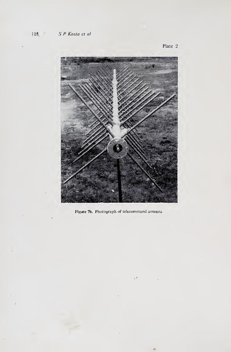
S P Kosta et al 1 It
Plate 2
Figure 7b. Photograph of telecommand antenna

The tracking system
M K SAHA, S KALYANARAMAN, S N PRASAD, R N TYAGI,
T K JAYARAMAN, M SAMBASIVA RAO and S G BASU ISRO Satellite Centre, Peenya, Bangalore 560 058
MS received 28 April 1977; revised 28 November 1977
Abstract. This study presents a complete description of the satellite tracking system used for Aryabhata. The total system consists of (i) an interferometry system to mea¬ sure the direction cosine angles of the satellite with respect to the ground station, (ii) a tone-ranging system to measure the range of the satellite and (iii) a Doppler system to measure the range rate of the satellite. The system accuracies obtained were ±10' of an arc in the direction cosine angles, ±T0 km in the range and ±6-6 m/s in the range rate.
Keywords. Satellite tracking system; interferometry system; tone-ranging system; Doppler system.
1. Introduction
The tracking system is an essential part of a ground station for obtaining the orbital
elements of any satellite. Since orbit degradation occurs under perturbing forces
such as drag due to atmospheric density, earth oblateness etc., it is necessary to
continuously track the satellite in order to update the orbital parameters.
Theoretically, six independent observations of a particular tracking parameter of
a satellite are sufficient to determine its orbit completely. However, due to inaccura¬
cies of measurement involved, more than one tracking parameter is usually measured
and weighting for the data of a particular parameter is given depending upon the
accuracy of measurement, for orbital computation purposes.
For Aryabhata, because of spacecraft constraints, no separate onboard tracking
package was installed. However, with the available onboard communication
packages (telecommand receiver and telemetry transmitter), three tracking systems
were developed and are described below.
(i) An interferometry system, to provide angular information of the satellite. It
uses the carrier component of the telemetry transmission as the beacon for
tracking purposes.
(ii) A tone-ranging system, to provide range. It uses the onboard communication
packages as transponder for the measurement of range.
(iii) A Doppler system, to provide range rate. It uses the onboard telemetry
transmitter carrier frequency as the beacon frequency for tracking putposes.
The three tracking systems were installed at SHAR and are being used to obtain
the tracking parameters of Aryabhata having a near circular orbit of 600 km altitude
119

120 M K Saha et at
at an inclination of 51° to the equatorial plane. The station at SHAR provides
tracking data for about 10 min for the satellite pass with a maximum elevation of 90°.
The data are recorded using a digital printer.
The tracking data are provided to the Post-Launch Operation Group for analysis.
The analysis consists of smoothing the data by a curve fitting procedure and then
using the smoothed data to up-date the orbital parameters of the satellite. The
following sections deal with the requirements, principles, design considerations and
performance of the tracking systems.
2. Choice of the systems
The systems conceived for Aryabhata are relatively simple compared to available
systems due to the limitations of spacecraft configuration and availability of resources
and time. The three tracking systems—interferometry, tone-ranging and Doppler
tracking, the last being a supplement to the first two—were decided upon to meet the
following requirements of accuracy:
direction cosine angle : ±6' of an arc;
range : ±1 km;
range rate : ±6-6 m/s.
Sophisticated interferometry systems capable of giving an accuracy of better than
^20" of arc in the direction cosine angles have been developed over the years by
many nations. This involves huge antenna structures providing a directive gain,
automatic electrical length measurement and control systems and an elaborate
calibration procedure (Nollet et al 1974).
For Aryabhata, as the requirement of accuracy was only ^6' of arc, it was
decided to go in for a simple interferometry system consisting of six omnidirectional
(turnstile) antennas with highly phase-stable foamflex cables to feed four pairs of
receivers located in the operator’s room.
The analysis indicates that with this simple system it is possible to meet the require¬
ment of the angular accuracy.
There are three widely used systems for the measurement of the range of a space¬
craft from the gound station:
(i) a coded ranging system,
(ii) a multiple continuous-wave-tone ranging system,
(iii) a hybrid of the above two.
These systems differ from each other in accuracy, acquisition time, maximum range
capability, and compatibility with other signals to be used with the ranging signal.
A coded ranging system cannot be used with the PCM telemetry signal of interest.
So, the choice is mainly between a multiple CW-tone ranging system and a hybrid
system. Analysis shows that the time required to acquire the hybrid signal is
inversely proportional to the signal-to-noise ratio (SNR) at the input, while in the
case of multiple CW-tone ranging system, it is independent of SNR. Though a
hybrid system can give better accuracy, it is more complex than a CW-tone ranging

The tracking system 121
system. Considering these, the latter was selected for ranging purposes (Kuwand
et al 1974; Peterson and Gupta 1965; Baghdady and Kruse 1965).
A two-way Doppler system with an onboard coherent transponder provides
better accuracies than a single way Doppler system, as onboard oscillator instability is
cancelled. However, for Aryabhata, a one-way Doppler system was selected because
a separate transponder could not be installed onboard due to various spacecraft
constraints like power, size and weight, and ground station constraints like
availability of resources, time and complexities involved.
3. Interferometry tracking system
3.1. The principle
This system is used to give the direction cosine of the satellite with respect to north-
south and east-west directions. In this system there are basically two receiving
antennas separated by a distance D (figure 1). For a distant target carrying a
beacon, the direction cosine p with respect to the line connecting the antenna is given
by
p = COS a = (f) \ / D, (1)
where A is wavelength of transmission, a is direction cosine angle, and <f> is phase
difference of the wave arriving at the two antennae expressed in a fraction of a cycle.
By partially differentiating (1), we get
and
dP = d^_d£ d^ p A D cf>’
da = COt a ~3A
. A
d_D
D
d4>
$ -
(2)
(3)
The sign of quantities in brackets indicates only the direction of errors involved
and in the worst case they become additive. Hence, for the worst case.
da — cot 8D
D
d<f>
<f> - (4)
Figure 1. Diagram showing the basic principle of the interferometry system

122 M K Saha et a l
It can be seen from (2) that the accuracy in the determination of p can be increased
by increasing D for a given error in the measurement of </>. But if D is increased
beyond A, there is an ambiguity in the determination of p, since <£ is cyclic for a path
difference of more than A. Hence, generally two or three pairs are provided in each
direction so that coarse, medium and fine accuracies are obtained and the ambiguity
in the fine channel can be resolved using medium and coarse channels.
3.2. System design considerations
The system conceived for Aryabhata has two pairs of antennae, in each of the two
orthogonal directions (N-S and E-W), one as a coarse channel and the other as a
fine channel. The following achievable errors were assumed before determining
the base-length.
(i) An error d<f> of ±7° in the measurement of phase difference, arising from
differential phase stability of the circuit and the phase jitter for a signal level
of —130 dBm.
(ii) An error <9A in the assumption of the wavelength of transmission amounting
to the frequency instability of the onboard transmitter plus Doppler shift in
frequency (±3-5 kHz).
(iii) An error dD in the determination of the distance between the antennae
(±2 mm).
Substituting in (4) the above errors and the requirement of accuracy in a of ±6'
of arc for 30° <a<90°, we found that a baseline separation of A for the coarse
channel and 25 A for the fine channel are required. Moreover, with these errors in the
coarse channel, it is possible to resolve the ambiguity in the fine channel (appendix 1).
antenna platform
test antenna platform
Figure 2. Geometry of the antenna field for the interferometry system

The tracking system 123
3.3. Antennae
The antenna field essentially consists of 6 antennae forming a total of 4 pairs of
antennae (figure 2). One antenna each in N-S and E-W directions is used as the
reference for both coarse and fine channels. Two dummy antennae are added for
symmetry. The antennae are of the turnstile type and are designed to have nearly
omnidirectional characteristics over a range of elevation angles between 30° and 90°.
The calculations were made for various values of d/A, where d\2 is the height of the
antenna over a reflective platform and are given in table 1. From the table it is
Table 1. Tracking antenna gain over isotropic antenna
d/X 0-5 0-7 0-9
Angle (deg.) P E P E P E from zenith dB dB dB dB dB dB
0 + 4-14 +4-15 + 3-81 + 3-81 -5-63 -5-63 15 +4-11 + 4-03 + 3-91 + 3-83 -3-53 -3-61 30 + 3-99 +3-93 + 3.95 +3-09 +0-59 -0-47 45 + 3-19 +0-47 + 4.15 + 1-43 + 3-61 +0-89 60 + 1T5 -3-79 + 3-15 -1-79 +4-35 -0-59 75 + 3-89 -12-41 -1-19 -9-71 +0-95 -7.57
p — pattern gain E = effective signal level including range variation
ref. coarse/fine
i-igure 3. Block schematic of the interferometry system for one channel

124 M K Saha et al
seen that for a d\A=0-7, the required gain pattern is achievable ensuring that
once the satellite is acquired, the signal does not fall for higher elevation angles
and the signal strength is fairly uniform.
The block schematic of the entire system is shown in figure 3. The special local
oscillator (SLO) provides two frequencies separated by 125 Hz and phase-locked to
each other. The signals from a pair of antennae are added and amplified in a
common channel, to keep the differential phase shift at a minimum. Using this
scheme, the phase difference which exists at the inputs of the pair of antennae is
transferred to 125 Hz signal appearing at the output of the square law detector,
relative to the reference 125 Hz . In this scheme, the error due to differential phase
shift between the channels is minimised.
3.4. Specifications
Antennae
Mounting
Base-length
Pattern gain
Polarisation
Locking sensitivity
Noise figure
Predetection BW
Phase lock loop noise bandwidth
(at 125 Hz)
Resolution of phase measurement
turnstile-nearly omnidirectional
non-steerable
A and 25 A at 137-44 MHz
3-8 dB to -1-2 dB; 90° >a>30°
circular
— 130 dBm
3 dB
15 kHz
2-5 Hz
001°
4. Tone-ranging system
4.1. The principle
In this system, the range of the satellite from the ground station is measured by
utilising the principle that an electromagnetic wave when propagated over a
distance experiences a delay. If the two way range is 2r and A is the wavelength,
the total phase delay suffered by the wave, expressed as a fraction of a cycle,
is given by
<f> + n = 2 r/A, (5)
where n is an integral multiple of 2n radians of phase shift suffered by the wave.
From (5) it can be noticed that the maximum unambiguous range obtainable depends
upon the frequency of the tone used for ranging; the lower the frequency, the higher
is the unambiguous range.

The tracking system 125
Figure 4. Block schematic of the tone ranging system
4.2. System design considerations
For a given inaccuracy in the measurement of <f>, increasing the tone frequency reduces
the error in r. For an unambiguous range of 4687-5 km and an accuracy of ^ 1 km,
four tones, 32 Hz, 160 Hz, 800 Hz, and 4000 Hz were selected. The required accuracy
is obtained at the highest tone and the ambiguity is resolved successively by the
lower tones (Habib et al 1964; Shaffer et al 1964). The lower tones, before they are
transmitted are up-converted to 4032 Hz, 4160 Hz and 4800 Hz and added to 4000 Hz
to conserve the bandwidth. These tones are transponded by the telecommand receiver
and telemetry transmitter onboard. The ground transmitting section consists of a
tone generator, an up-converter of lower tones and an AM transmitter. The ground
receiving section consists of an input filter, tone filters, phase correcting networks, a
digital processor, display and an interface to printer. The block schematic of the
tone ranging system is given in figure 4.
The received 4 kHz tone is extracted from the composite tones using a phase locked
loop. The phase correction networks are used for correcting any offset in the phase
delay. With the help of transmitted and received tones, the digital processor generates
a pulse whose width is the measure of range. This pulse is fed to a counter as a
gate to give the range directly.
4.3. System specifications
Maximum range
Tone frequencies
Phase jitter allowed in lower tones
Phase jitter in 4 kHz tone
Accuracy in the range measurement
Uplink
Downlink
4687.5 km
32 Hz, 160 Hz, 800 Hz and 4000 Hz
±30° (3<r value)
±10° (3cr value)
±1’0 km (3cr value)
AM
PM (deviation=1 rad.)

126 M K Saha et al
5. Doppler tracking system
5.1. The principle
The range rate of the satellite with respect to the ground station is determined by
the Doppler technique. The Doppler frequency is given by fd = VfJC if V<C,
where V is the radial velocity of the satellite, f0 is the transmitter frequency and C
is the velocity of light. Thus, to determine the Doppler frequency it is necessary that
the transmitter frequency is known precisely.
5.2. System design considerations
The telemetry carrier working at 13744 MHz is used as the beacon signal. This
necessitated a highly stable frequency source for telemetry transmission with a long
term stability of 1 x 10⁻⁶ and a short teim stability of 1 X 10“8 over the average radio
visibility duration of 10 min. At this carrier frequency, the Doppler shift ranges
between ±4 kHz for a circular orbit of 600 km altitude.
The ground segment (figure 5) consists of an antenna with a preamplifier and a
double superheterodyne receiver. The second IF is at a frequency of 20 kHz which
also acts as a bias frequency for the Doppler to swing in either direction by ±4 kHz.
Since any instability in the local oscillators used in the receiver affects the accuracy
I F. = Intermediate frequency
Figure 5. Block schematic of the Doppler tracking system
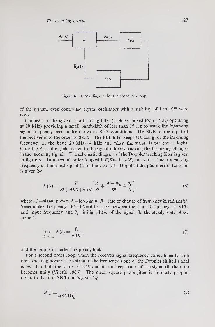
The tracking system 127
Figure 6. Block diagram for the phase lock loop
of the system, oven controlled crystal oscillators with a stability of 1 in 1010 were
used.
The heart of the system is a tracking filter (a phase locked loop (PLL) operating
at 20 kHz) providing a small bandwidth of less than 15 Hz to track the incoming
signal frequency even under the worst SNR conditions. The SNR at the input of
the receiver is of the order of 0 dB. The PLL filter keeps searching for the incoming
frequency in the band 20 kHz:j=4 kHz and when the signal is present it locks.
Once the PLL filter gets locked to the signal it keeps tracking the frequency changes
in the incoming signal. The schematic diagram of the Doppler tracking filter is given
in figure 6. In a second order loop with i7(S,)=l+a/S', and with a linearly varying
frequency as the input signal (as is the case with Doppler) the phase error function
is given by
HS) =_5_p + + V S2+AKS+aAKlS* S2 5.
(6)
where ^42=signal power, if=Hoop gain, R=rate of change of frequency in radians/s2,
.S=complex frequency, W— W0—difference between the centre frequency of VCO
and input frequency and 0o=initial phase of the signal. So the steady state phase
error is
lim (t) = JL, (7) t-> co aAK
and the loop is in perfect frequency lock.
For a second order loop, when the received signal frequency varies linearly with
time, the loop acquires the signal if the frequency slope of the Doppler shifted signal
is less than half the value of aAK and it can keep track of the signal till the ratio
becomes unity (Viterbi 1966). The mean square phase jitter is inversely propor¬
tional to the loop SNR and is given by
— 1
2(SNR)^. (8)

128 M K Saha et a l
As the frequency is measured by 02(O> there is a frequency error when measurement
is made over an integration time Tt. The error in /is
A /= 1
47rTi(SNR)L
5.3. Specifications
Sensitivity
Antenna
IF bandwidth
PLL bandwidth
-130 dBm
Same as interferometry
10 kHz
15 Hz
(9)
6. Performance
6.1. Interferometry
The interferometry system became functional two weeks after the launch of
Aryabhata. The spin of the satellite around 50 rev/min caused amplitude
fluctuations in signal strength. This caused an increase in phase jitter necessitating
a smoothing of the data before putting them into actual use. Fixed offsets
in the data were removed after analysis of the data pertaining to various orbits.
An accuracy of ^10' of an arc was achieved against the design target of ^ 6'
of arc. One representative curve of the observed data is given in figure 7. Apart
from the errors in the system there are many other sources of error such as
ionospheric refraction of the order of 0-05° to 0-2° at 45° elevation under average
ionospheric conditions, antenna misalignment in N-S and E-W directions of the
order of 20" of arc, and ground levelling and ground reflections of the signal.
However, corrections based on the predictions of the index of refraction can be
applied. In the initial phase, the entire data were used to generate coarse orbital
elements but once they became better defined, the data pertaining only to near
zenith were used to refine the orbital elements. In this zone, the errors due to the
ionosphere can be minimised to less than 20" of an arc. During installation,
the distance between the centres of the antennae of the N-S and E-W lines was deter¬
mined using tellurometers and theodolites. In practice, the problems of installing
the system are greater than those of developing it.
Some improvements in the installed system have been contemplated to achieve
better accuracy. These include provision of better antenna gain, reduction of the
differential phase shifts and a better calibration procedure using an aircraft with a
flash and a beacon.
6.2. Tone-ranging system
The tone-ranging system was calibrated with the satellite for zero distance. The
system was put into operation 15 days after launching. The tone-ranging data are
straightforward and can be used as such, as the print-out gives the range in kilometres.

phase angle
( d
eg
)
The tracking system 129
Figure 7. Comparison between the observed and predicted phase angles for the interferometry system
Figure 8. Comparison between the observed and predicted range for the tone-ranging system
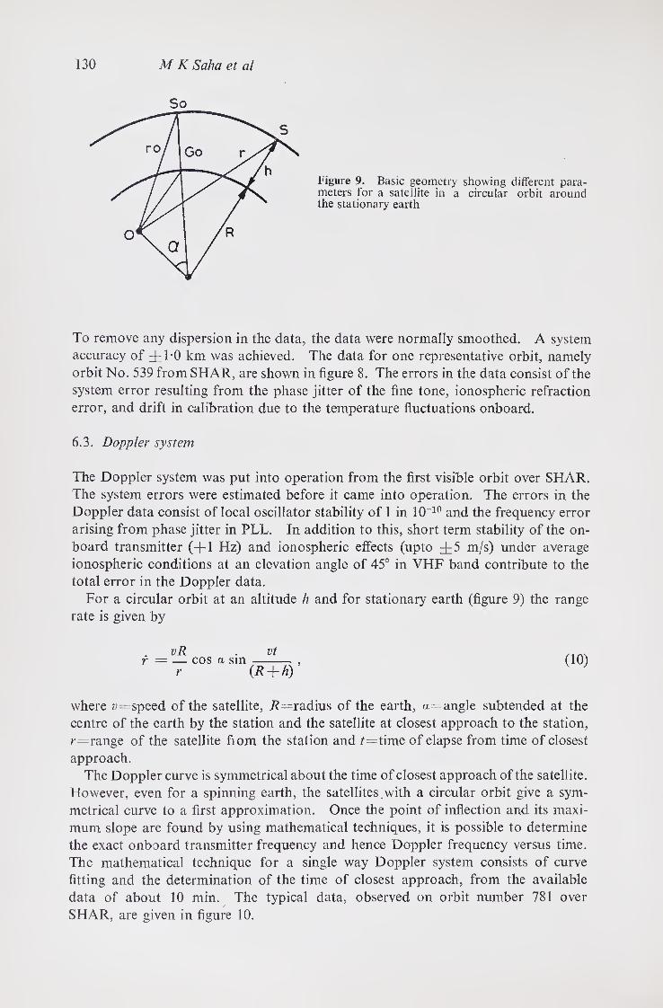
130 M K Saha et al
Figure 9. Basic geometry showing different para¬ meters for a satellite in a circular orbit around the stationary earth
To remove any dispersion in the data, the data were normally smoothed. A system
accuracy of ±1-0 km was achieved. The data for one representative orbit, namely
orbit No. 539 from SHAR, are shown in figure 8. The errors in the data consist of the
system error resulting from the phase jitter of the fine tone, ionospheric refraction
error, and drift in calibration due to the temperature fluctuations onboard.
6.3. Doppler system
The Doppler system was put into operation from the first visible orbit over SHAR.
The system errors were estimated before it came into operation. The errors in the
Doppler data consist of local oscillator stability of 1 in 10-10 and the frequency error
arising from phase jitter in PLL. In addition to this, short term stability of the on¬
board transmitter (-f 1 Hz) and ionospheric effects (upto ±5 m/s) under average
ionospheric conditions at an elevation angle of 45° in VHF band contribute to the
total error in the Doppler data.
For a circular orbit at an altitude h and for stationary earth (figure 9) the range
rate is given by
r = — cos a sin -, (10) r (R + h)
where v— speed of the satellite, R=radius of the earth, a= angle subtended at the
centre of the earth by the station and the satellite at closest approach to the station,
/-=range of the satellite fiom the station and time of elapse from time of closest
approach.
The Doppler curve is symmetrical about the time of closest approach of the satellite.
However, even for a spinning earth, the satellites.with a circular orbit give a sym¬
metrical curve to a first approximation. Once the point of inflection and its maxi¬
mum slope are found by using mathematical techniques, it is possible to determine
the exact onboard transmitter frequency and hence Doppler frequency versus time.
The mathematical technique for a single way Doppler system consists of curve
fitting and the determination of the time of closest approach, from the available
data of about 10 min. The typical data, observed on orbit number 781 over
SHAR, are given in figure 10.

The tracking system 131
4 5 6 7 8 9 10 11 12 13 14 15
time (min)
Figure 10. Comparison between the observed and predicted range rate for the Dopier tracking system
Table 2. Tracking systems accuracies
Parameter Systems Design goal (3 o-)
Achieved accuracy (3 a)
Direction cosine angle
Interferometry ±6' of arc ±10' of arc
Range Tone ranging ±1 km ±1 km Range rate Doppler ±6-6 m/s ±6-6 m/s
7. Conclusions
The satellite tracking systems installed at SHAR, which are the first of their kind
in India, have provided tracking data which have been used to generate satellite
ephemeris for Aryabhata. Table 2 indicates the achieved tracking accuracies against
the design goals.
It should be emphasised that for improved accuracy in tracking by electronic
systems, the frequency of operation should be above 1 GHz. In addition a good
calibration system for interferometry is essential.
Acknowledgements
We would like to thank Prof. U R Rao for his encouragement throughout the course
of this work. Our thanks are also due to the antenna group and Messrs D. John,

132 M K Saha et al
M K Nair, K N Madhavan and N V Shivprasad for their valuable contributions
during the development and installation of the systems.
Appendix 1
The error in the direction cosine angle is given by
da = cot a 'aA -f ££ + dA .A ^ D + cf>
Coarse channel : D/A = 1,
da = cot a (2T X 10_5+90x 10^5~4-1942X 10-5).
Fine channel: D/A = 25,
da = cot « (2-1 x 10⁻⁵+3-6x 10⁻⁵+77x 10-5).
The accuracy of the system is given by the fine channel. With the error in the coarse
channel, it should be possible to resolve the ambiguity between the two adjacent
ambiguous direction cosine angles in D=25A channel.
Table 3. Error calculation for various angles of arrival a
da
a (in degrees)- Coarse channel Fine channel
89 ± 11° ±2-6°
70 ± 1-2° ±3'
50 ± 1-5° ±3-5'
30 ± 2-2° ±6'
10 ± 5-2° ± 15'
a (in degrees) Interval between adjacent
ambiguous angles
10 ± 10°
30 ± 4°
50 ± 3°
70 ± 2-4'
90 (zenith) ± 2-3'

The tracking system 133
References
Baghdady E J and Kruse K W 1965 IEEE Trans. Commun. Technol. 13 4 Habib E J, Kronmiller G C Jr, Engels P D and Franks H J Jr 1964 NASA TN D 2093 Kuwand R, Tand J, Harund T and Fuke F 1974 NEC Research and Development Rep. No. 33 Nollet M, Faillie V G, Goessl H and Hounam D 1974 Electr. Commun. 49 3 Peterson W D and Gupta S C June 1965 IEEE Trans. Aerosp. Navig. Electron. Shaffer H W, Kahn W D, Bodin W J Jr, Kronmiller G C, Engels P D and Habib E J 1964 NASA
TN D 2139 Viterbi A J 1966 Principles of coherent communications (New York: McGraw Hill)


The structure
A V PATKI ISRO Satellite Centre, Peenya, Bangalore 560 058
MS recived 28 April 1977; revised 21 November 1977
Abstract. The design, analysis and testing methods of the Aryabhata satellite struc¬ ture are briefly presented. The general requirements and constraints which formed the basis of the design of the structure are explained. The theoretical and experi¬ mental studies conducted to evaluate the structural behaviour under various environ¬ mental loads expected during ground operations and during flight are also described. The salient features of the fabrication procedures and the details of physical para¬ meters are presented. Finally the evaluation of the structure is made on the basis of the results of ground tests and the flight performance.
Keywords. Satellite structure; structural design; structural design/structral confi¬ guration.
1. Introduction
One of the basic subsystems of a satellite is its structure. The design aims at a
structure that will meet the known functional requirements of the satellite such as
power and thermal control, look-out windows for sensors, and magnetic cleanliness
with minimum weight and maximum reliability. On the basis of experience of other
countries reported in the literature, one can evolve some guidelines as regards the
selection of the overall structural configuration and materials. The structural design,
however, is highly dependent on the mission requirements and the launch vehicle
characteristics. In the Aryabhata structural design, an attempt was made to arrive
at a reasonable compromise between the design objectives of minimum weight and
maximum reliability satisfying all the functional requirements and constraints.
Detailed theoretical and experimental studies were made to achieve this objective.
Analytical techniques were employed for the theoretical analysis of the structure
while the experimental studies, which formed the final basis for qualification, were
conducted using available facilities. The experience now available in the country in
aircraft structural fabrication was fully exploited for the fabrication of the Aryabhata
structure.
The requirements and constraints on the Aryabhata structure are detailed in §§ 2
and 3. The analysis, testing and fabrication aspects are described briefly in §§ 4, and
5, followed by a brief statement of the performance of the structure on the basis of
the results of ground tests and flight performance.
2. The functional and other requirements on the structure
The satellite structure, apart from serving as a safe container for the various
135
P. (C)—2

136 A V Patki
subsystem packages, has also to meet several other requirements. The surface area of the structure, for example, has to meet the dual requirements of power and thermal control; the solar panels need to be fixed to the outer surface of the Aryabhata
structure, and the passive thermal control system required some free exposed area for thermal treatment. To keep power fluctuations to a minimum, irrespective of the orientation of the satellite in inertial space, a quasi-spherical shape for a spinning satellite is ideal. These requirements had a significant influence on the choice of the shape of the structure. The structure was also required (i) to provide the necessary radiation shielding to the packages inside the satellite, (ii) to possess not more than the allowable maximum electrical resistance (less than 2-5 milliohms between the deck plate and skin, and less than 10 milliohms between any line points on the deck plate), and (iii) to be magnetically clean. Table 1 gives a comprehensive list of all such general requirements of the satellite structure.
The overall size of the structure was dictated mainly by the dynamic envelope of the launch vehicle heat shield. Spin stabilization of Aryabhata called for fixing the moment of inertia ratio (7Z//*) around 1-4. This requirement had a significant influence on the choice of the structural configuration.
One of the major considerations in the design of the structure is the loads acting on it. The satellite is subjected to the static and dynamic, handling and transportation loads on the ground; the severe vibratory, shock and static acceleration loads during lift-off and separation; and the thermal and centrifugal loads in orbit. The details of these loads are given in table 2.
Table 1. General requirements of satellite structure
A. Functional requirements
Housing all instruments and experimental packages
Providing windows/cut-outs for sensors
Supporting surface for solar panels
Protecting the instruments from radiation
Proper interface with the launch vehicle
Provision for ground handling, antennae and jet nozzle mounting etc.
Electrical contact resistance requirements (2-5-10 milliohm)
Provision for thermal control
B. Other requirements!constraints
Minimum weight
Size to suit heat shield dynamic envelope
Surface area: thermal and power considerations
Material: magnetic cleanliness, availability and cost
Maximum accessibility
Fabrication considerations
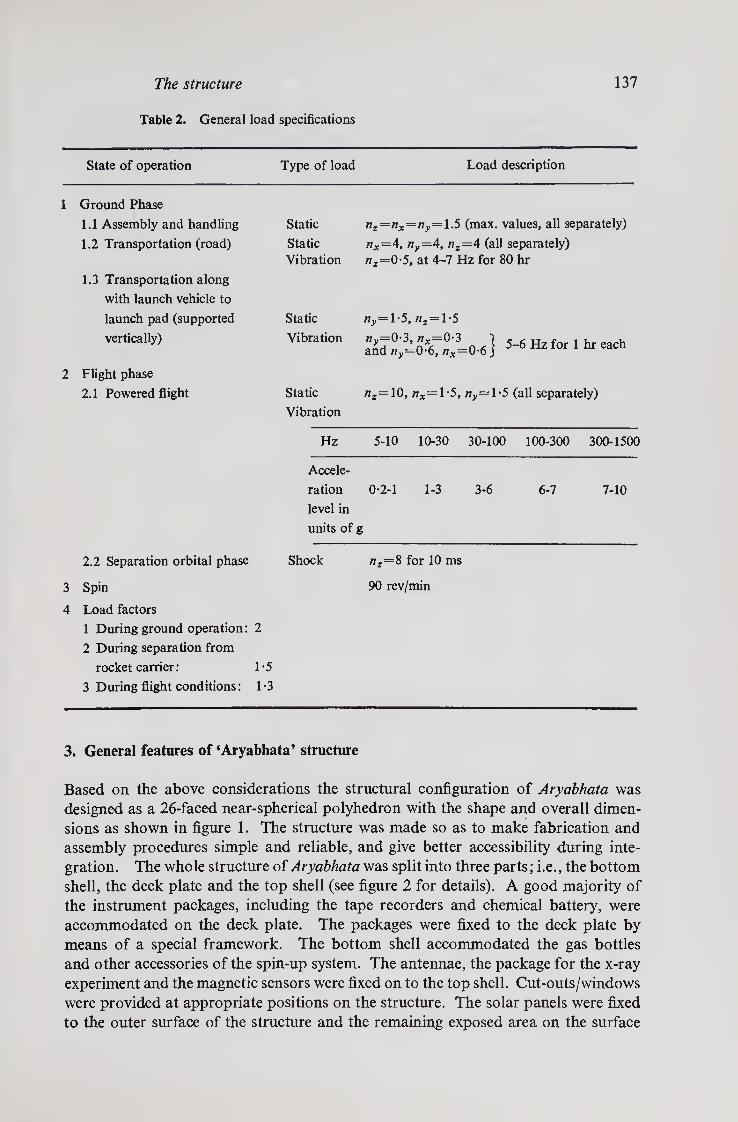
The structure 137
Table 2. General load specifications
State of operation Type of load Load description
Ground Phase
1.1 Assembly and handling Static nz=nx=ny—1.5 (max. values, all separately)
1.2 Transportation (road) Static nx=4. ny=4, nz=A (all separately) Vibration nz=0-5, at 4-7 Hz for 80 hr
1.3 Transportation along
with launch vehicle to
launch pad (supported Static wy=l-5, h2=T5
vertically) Vibration "S°,=S€t=0-6} 5-6 Hz fori hr each
Flight phase
2.1 Powered flight Static
Vibration
nz=10, /i*=T5, wy=l-5 (all separately)
Hz 5-10 10-30 30-100 100-300 300-1500
Accele¬
ration
level in
0-2-1 1-3 3-6 6-7 7-10
units of g
2.2 Separation orbital phase Shock «z=8 for 10 ms
Spin 90 rev/min
4 Load factors
1 During ground operation: 2
2 During separation from
rocket carrier: 1-5
3 During flight conditions: 1-3
3. General features of ‘Aryabhata’ structure
Based on the above considerations the structural configuration of Aryabhata was designed as a 26-faced near-spherical polyhedron with the shape and overall dimen¬ sions as shown in figure 1. The structure was made so as to make fabrication and assembly procedures simple and reliable, and give better accessibility during inte¬ gration. The whole structure of Aryabhata was split into three parts; i.e., the bottom shell, the deck plate and the top shell (see figure 2 for details). A good majority of the instrument packages, including the tape recorders and chemical battery, were accommodated on the deck plate. The packages were fixed to the deck plate by means of a special framework. The bottom shell accommodated the gas bottles and other accessories of the spin-up system. The antennae, the package for the x-ray experiment and the magnetic sensors were fixed on to the top shell. Cut-outs/windows were provided at appropriate positions on the structure. The solar panels were fixed to the outer surface of the structure and the remaining exposed area on the surface

138 A VPatki
was used for the purpose of thermal control. The thin structural panels served as radiation shields, as a sensor base, and also provided for the necessary thermal control surface. To meet the interface requirements with the launch vehicle, four lugs were provided at the bottom of the satellite structure.
4. Theoretical analysis and testing of structure
To arrive at a viable and efficient structural design, a few cycles of iteration involving design, analysis and/or testing followed by a careful redesign are essential. In the present case, this procedure was followed within the severe limitations imposed by the project time schedule. On the basis of loads specified and other design inputs available from time to time, fairly detailed theoretical analysis and experimental
Figure 1. Satellite geometry showing dimensions of the overall structure without solar panels and skin.
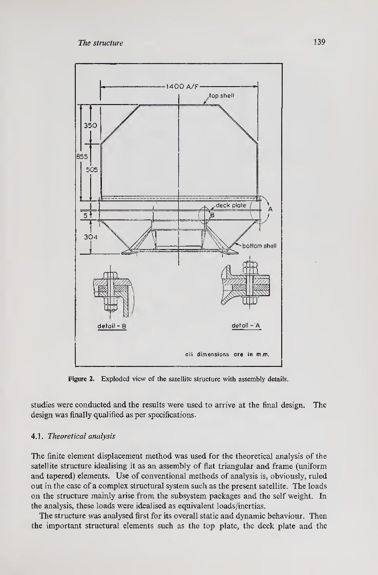
The structure 139
studies were conducted and the results were used to arrive at the final design. The design was finally qualified as per specifications.
4.1. Theoretical analysis
The finite element displacement method was used for the theoretical analysis of the satellite structure idealising it as an assembly of flat triangular and frame (uniform and tapered) elements. Use of conventional methods of analysis is, obviously, ruled out in the case of a complex structural system such as the present satellite. The loads on the structure mainly arise from the subsystem packages and the self weight. In the analysis, these loads were idealised as equivalent loads/inertias.
The structure was analysed first for its overall static and dynamic behaviour. Then the important structural elements such as the top plate, the deck plate and the
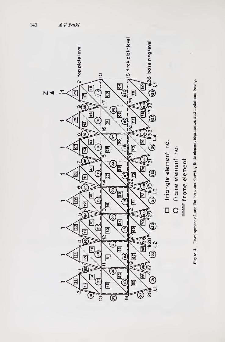
140 A VPatki
6 c
c cd
£ o> a>
QJ
cr> c o u
6 c
c c CD CD
E £ — CD CD
CD <D £ o l.
£ o L.
□ o i i
Fig
ure
3.
Dev
elopm
ent
of
sate
llit
e st
ruct
ure
show
ing f
init
e el
emen
t id
eali
sati
on a
nd n
od
al n
um
ber
ing.

The structure 141
antennae were studied in detail. The boundary condition for analysis assumed full fixity at the four lug positions.
Figure 3 gives, as a demonstrative example, the development of the surface of the satellite structure showing the finite element idealisation with element and node numbering. It may be worthwhile to mention here that the handling of the matrix equations, which the application of the finite element method finally leads to, needs special purpose computer programmes for reducing computer time and storage. Matrix properties such as symmetry, banded nature and sparseness need to be fully exploited. An automatic node numbering scheme was used when necessary for the re-numbering of nodes of the finite element analytical model to achieve minimum bandwidth of mass and stiffness matrices. Special purpose solution and eigen value programmes were employed for bending and vibration studies.
The analysis was carried out for static deflections and stresses for different loads, i.e., lateral and longitudinal acceleration loads, and other loads due to spin and non- uniform heating in orbit. The stresses and displacements were found to be well within the allowable limits. The axial/in plane compression induced in the structural members was found to be too small to have any significant influence on their stiffness. The local and overall buckling behaviour of the structural elements was also calcu¬ lated and the high margin of safety against buckling ascertained.
Vibration studies were also conducted on the structure. The results were used both to provide design data and as an aid to experimental studies. The frequencies
Table 3a. Some results of theoretical analysis (statics)
Description of the part
Loading
Maximum displacements
Direction Magnitude (mm)
Maximum stress
(kg/mm2)
Top part Lateral X -1-46 5-14 nx=ny=—8 y -1-46
Z -1-08
Axial X -0-03 «z= —13 y -0-03 0-62
Z -001
Thermal X -0-25 y -0-25 0-46 Z -0-37
Thermal and spin X 0-25 (90 rev/min) y 0-25 0-57
Z -0-38
Bottom part Lateral X -0-90 nx=ny= — 8 y -0-94 5-79
Z 1-24
Axial X -0-07
s
N II 1 u>
y 0-08 9-36 Z -014
Complete Lateral X -0-58 structure nx=ny——8 y -0-60 11-04
Z -0-38
Axial X 0-01
a N II 1 u>
y 0-01 16-44 Z 9-23*
*At centre of top plate

142 A V Patki
Table 3b. Some results of theoretical analysis (dynamics)
Description of the part
Boundary Natural frequency (Hz) in different modes condition 1 2 3 4 5 6
Top trapezoidal panels
Simply supported
Rectangular panels
Simply supported
Top octagonal plate Simply supported
Bottom trapezoidal panels
Simply supported
Antenna Cantilever
Top part of structure Clamped at deck plate level
Complete structure Clamped at lugs
34.0 71-0 93-0
23-0 56-0 90-0
26-0 73-0 134-0
46-0
35-3
103-0
134-3
127-0
324-3
36-98 37-0 41-2 41.3 54-6 54-6
26-0 37-0 41-0 55-0 56-0 61-0
of the unstiffened structural panels, for example, were found to be close to the whole structure fundamental frequency which is known to be undesirable for sound dynamic performance. The stiffening of the panels raised these element natural frequencies to the desired levels.
The onboard antennae vibration performance, the tip deflections and the stresses under specified root excitations were studied in detail. These confirmed the margin over dynamic envelope of the heat shield of the rocket carrier. Some important results from the theoretical analysis are displayed in tables 3a and 3b. The results for stresses and displacements for only a few important loading conditions are presented. Detailed analysis of the top part and bottom part of satellite was performed separately before the final analysis of the whole satellite structure. The results of these analyses showed, in general, that the stresses were well within the permissible limits. The results of free vibration studies are presented in table 3b. The structural element frequencies which were initially found to be rather close to the system frequencies, were raised by providing suitable stiffeners.
4.2. Experimental studies
Apart from the theoretical studies described above, detailed experimental studies were conducted on the satellite structure both in the developmental phase and later during the final qualification. Table 4 summarises the various tests conducted on the satellite structure to simulate the static and dynamic loads expected on the satellite at different stages such as ground handling, transportation, launching and orbital life.
These test specifications were based mainly on the launch vehicle data. The proce¬ dure for testing was arrived at after considering the nature of specifications and the type of test facilities available in India. Thus, the static acceleration loads were simulated using a whiffle tree system of loading. The dynamic tests were done mainly using sinusoidal sweep test on an electro dynamic shaker. A road test was conducted to simulate the low frequency vibratory loads during transportation. The satellite was also tested on the spin table for different spin rates (see figure 4, plate 1).

The structure 143
Table 4. Structure Itests on Aryabhata
Test What it simulates Test conditions
Static tests Handling tests Ground handling loads 3 g
Separation test Shock load during separation 12 g
Lateral axis test Loads during transportation 8 g
Longitudinal axis loading test Orbital injection 13 g
Dynamic tests Lateral axes vibration tests > i Dynamic loads during transpor- 5 to 1500 Hz, 0-2 to 10 g Longitudinal axis test J i tation and orbital injection sweep rate: 0-5 octaves/min
Transportation test Transportation from Cosmo¬ drome to launch pad
Road test: truck speed = 20 km/hr
duration =2 hr
Spin test Load due to spin during orbital flight
5 min each at 60, 90 and 101 rev/min.
4.3. Test procedure and results
The test specifications and the corresponding load factors are included in table 2. The first series of tests (static as well as dynamic) were on a developmental (or ‘experimental’) model. These tests were useful to gain experience in the testing techniques and also for obtaining some preliminary design data.
Detailed structural tests were then conducted on a mechanical mock-up which simulated the satellite in all its mechanical properties. The spin test on a spin table was conducted, followed by vibration tests and static tests. The low frequency vibration test was simulated later by a road test as shown in figure 5. During this test the input acceleration levels were measured and the peak input acceleration level was within 1 g. Inspection of the satellite after the test showed no damage to the structure. The model was later transported to the USSR, mated with the rocket to ensure mechanical compatibility and brought back and inspected to check for any damage due to transportation loads.
Vibration tests on prototype-I were conducted using an electrodynamic shaker as shown in figure 6 (plate 2). Initially, a resonance search test was conducted along the three axes, X, Y and Z to determine the natural frequencies of the structure. The acceleration levels at a number of stations on critical sub-system boxes and at important points on the structure were recorded. A special fixture was used for the Z-axis vibration test and a stiffened plate fixture for X and Y axes tests. The resonance search test was followed by resonance dwell tests at critical resonance frequencies. Some important results obtained during resonance search tests are listed in table 5. The vibration test brought out certain minor inadequacies in the dynamic properties of the structure. For example, near the top octagonal plate, the transmissibility level was found to be very high and hence it needed stiffening. Certain other modifications such as strengthening the tape recorder fixing table, improvements in the cable harness, etc., were also made.

144 A VPatki
accelerometer on the lug low frequency vibration
fixture
ampex make power FM tape recorder-, supply
generator
Figure 5. Schematic diagram of the set-up for the transportation test on the satellite.
Table 5. Some results from the vibration tests (Resonance esarch test)
Axis
Maximum trans- missibility
level (B )
Frequency (Hz) at
^max Accelerometer location of
test before after before after modifi- modifi- modifi- modifi- cation cation cation cation
Centre of top octagonal panel X 8-7 144-0
y 6-7 17, 75 120
Z >10 11-0 60, 80
200
125
Top octagonal edge X 5-0 15, 142
y 16-6 6-0 130 15 Z 4-0 4-6 140 13
On antenna tip X 11-4 15-40 95-170
y 100 17. 34 120, 280
Z 100 32, 140
On horizontal angle of deckplate framework X 12-7 17, 120
180 On the X-ray package box (top) z 15-0 72
X 11-5 75
y 9-0 67 On nozzle tip Z 20-0 100-105
On box EX 13 (deck plate centre) X 12-5 85
y 22 83 z 5-8 75
Natural frequencies Mode 1 2 3 4 5 6
Frequency (Hz) 32(z) 38(z) 42(L) 53(L) 64(z) 67(L) (z) Axial vibration (L) Lateral vibration

The structure 145
Figure 7. A typical diagram showing the results of the vibration test on the proto-III model
Moreover, since a later model (Prototype-Ill) was fitted with a different version of the bottom shell, qualification of this for structural loads was necessary. Hence, a sinusoidal sweep test was conducted after making the required modifications. The results of these tests showed that the satellite design was sound against dynamic loads. A typical graph showing the measured response is shown in figure 7. This provides a good estimate of various transmissibility levels (ft) with respect to the corresponding frequencies at a particular point.
The static tests were conducted on Prototype-I as per the specifications shown in table 2. The schematic diagram of the whiffle tree system of loading used for simu¬ lating the static acceleration loads is shown in figure 8. This system of loading applies the load on the satellite at individual points at various planes of the satellite. Through levered linkages all the loading points are connected and coupled to the final loading system. The accuracy of the load distribution was checked by means of load cells located at selected positions. During the tests, strains were measured at different points on the structure. The measured strains and the results of the detailed inspection after the test indicated that the structure was quite safe against static loads. The maximum stress was 650 kg/cm2 which was well within the design stress. The results of the static tests conducted to simulate the separation shock load and the handling loads also showed good margins of safety.
Thus the results of different structural tests together with those from the theoretical analysis established the confidence in the design.
5. Materials and fabrication
Apart from the primary consideration of high strength/weight ratio, the structural materials used in the satellite have also to be non-magnetic, as the presence of magne¬ tic materials affects the accuracy of the onboard magnetic sensors. Further, the
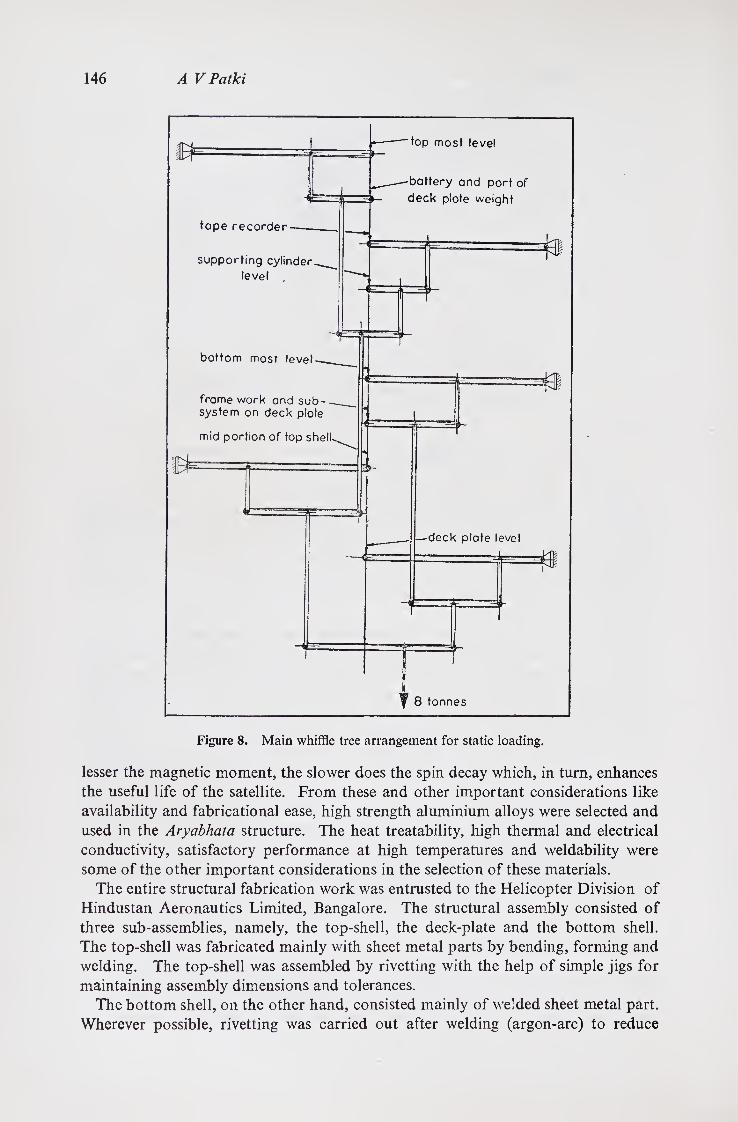
146 A V Patki
lesser the magnetic moment, the slower does the spin decay which, in turn, enhances the useful life of the satellite. From these and other important considerations like availability and fabricational ease, high strength aluminium alloys were selected and used in the Aryabhata structure. The heat treatability, high thermal and electrical conductivity, satisfactory performance at high temperatures and weldability were some of the other important considerations in the selection of these materials.
The entire structural fabrication work was entrusted to the Helicopter Division of Hindustan Aeronautics Limited, Bangalore. The structural assembly consisted of three sub-assemblies, namely, the top-shell, the deck-plate and the bottom shell. The top-shell was fabricated mainly with sheet metal parts by bending, forming and welding. The top-shell was assembled by rivetting with the help of simple jigs for maintaining assembly dimensions and tolerances.
The bottom shell, on the other hand, consisted mainly of welded sheet metal part. Wherever possible, rivetting was carried out after welding (argon-arc) to reduce

The structure 147
Table 6. Physical parameters
Overall weight of the structure (without fasteners) 93-7 kg
CG height (from base) 414-6 mm
Moments of inertia (theoretical) Ixx 24-54 kg m
Iyy 24-57 kg m
Izz 28-74 kg m
Total surface area 62,265 cm2
Minimum projected area 13,800 cm2
Area covered by solar cells 36,800 cm2
Overall height 1,164 mm
Equivalent diameter for structure 1,590 mm
Tip to tip distance with antennae 2,149 mm
Dynamic envelope of antenna 2,190 mm
shrinkage and the shrinkage stresses on the rivets. A welding jig was designed and fabricated specially for this purpose giving due allowances for welding shrinkages.
To cater to the requirements of the thermal design, the parts were given necessary surface treatments (anodising, polishing etc.,) before assembling. Aircraft standards were followed for dimensional tolerances, welding and rivetting and material inspec¬ tion of structural components. The details of the physical parameters of the satellite structure (flight model) are listed in table 6.
6. Concluding remarks
To summarise, the structural design of the satellite Aryabhata satisfied all the func¬ tional and other requirements. The cut-out and other provisions fully met the needs of different sub-systems and of integration. No special problems were encountered during integration, assembly, handling and mating operations. The actual flight performance of the satellite has proved the soundness of the design. The good magnetic cleanliness of the structure, for example, has helped to extend the useful life of the satellite by greatly slowing the rate of spin decay.
Acknowledgements
The entire work mentioned here was carried out towards the fulfilment of the project Aryabhata by the members of the structures group of ISAC. The author acknow¬ ledges the contributions from the various members of the project team. In particular, thanks are due to Prof U R Rao for overall guidance and the opportunity to publish this paper.

.
-

The structure 149
Plate 1
Figure 4. Satellite on the spin table

150 A VPatki
Plate 2
Figure 6, Satellite on the vibration table

System integration
V A THOMAS, M N SATHYANARAYAN, V R KATTI, A A BOKIL, N R DATHATHRI, G MOHANAKRISHNAN, K PATTABHIRAMAN, T K GOSWAMI, T L DANABALAN and I SELVARAJ ISRO Satellite Centre, Peenya, Bangalore 560 058
MS received 8 July 1977; revised 16 January 1978
Abstract. The paper discusses the various aspects of satellite integration. A detailed plan is given for both mechanical and electrical integration of Aryabhata, elucidating the integration procedures and practices which were evolved to cater to the various types of interface requirements between the different onboard subsystems as well as between the spacecraft and the rocket carrier.
Keywords. Satellite integration philosophy; system layout; mechanical integration; electrical integration; testing philosophy.
1. Introduction
The fundamental task of integration of Aryabhata was to provide the mechanical assembly and electrical interconnections for the various subsystem units to mould them into an electrically compatible, mechanically rigid and reliable system. The purpose of total integration was to ensure that all hardware would successfully func¬ tion as an integrated system to achieve the mission objectives of Aryabhata.
1.1. Integration process and philosophy
The process consisted of mechanical and electrical integration, qualification testing of the basic design using the engineering, mechanical and electrical prototype models and acceptance testing of the workmanship using the flight model. Qualification and acceptance considerations demanded an elaborate study on the interactions between the various subsystems including the experiments, interaction between the spacecraft and the launch vehicle and also the interactions between the subsystems and the environment to which they were likely to be exposed.
Each subsystem carried on the spacecraft had a large number of general interface requirements which normally could be put into the following categories.
(a) Mechanical interfaces generated by the constraints on size, weight, location, type of mounting, centre of gravity, moment of inertia and dynamic balance.
(b) Environmental interfaces based on requirements of thermal, vacuum, vibra¬ tion and shock mounting.
(c) Electrical interface based on requirements of voltage, current, noise tolerance, electromagnetic interference (EMI) compatibility, electrical interconnections and connector types.
151

152 V A Thomas et al
(d) Functional interfaces based on the requirements of alignment, stability, data calibration and tuning.
In addition, the following interfaces were also considered for the successful com¬ pletion of the prelaunch and launch phase operations.
(a) Spacecraft—ground support equipment interfaces based on the requirements of pre-launch and launch phase electrical checkout and handling operations and service points for filling the gas bottles of the spin-up system.
(b) Spacecraft—launch vehicle interfaces based on the requirements of electrical interconnections between the satellite and the launch vehicle including sepa¬ ration system and the heat shield envelope.
2. System layout
After a series of critical reviews on the subsystems and the structure, the subsystem layout was designed wherein the following considerations were taken into account.
2.1 Mechanical and environmental considerations
(a) Provision of a configuration permitting the separate development and quali¬ fication of the experimental packages and technological subsystems.
(b) Desirability of packaging the electronic subsystems in units of standard dimen¬ sions.
(c) Rational location of subsystems to achieve adequate load and heat paths and to minimise weight concentration.
(d) Compactness and peripheral distribution of the subsystem units to keep the values of the physical parameters such as the moment of inertia, centre of gravity within the specifications.
(e) Static and dynamic balancing from the point of view of stabilisation. (f) Accessibility, replaceability and serviceability of all the subsystems and sub-
assemblies. (g) Provisions for ground handling and ground operations. (h) Adequate support for the subsystems with a minimum vibration and shock
transmissibility. (i) Contribution of the subsystem packages to the stiffening of the structure. (j) Adequate margin for weight growth with a reasonable minimum of 25 %. (k) Achieving a reasonably high value of packing factor that is feasible under
given constraints for the physical parameters. (l) Provisions for the thermal control of each of the subsystems to maintain the
thermal environment of the spacecraft within the thermal specifications.
2.2. Functional and electrical considerations
(a) Functional grouping of subsystems to minimise cabling paths and develop¬ ment, assembly and testing problems.
(b) Effecting proper physical separation between the EMI sources and susceptible subsystems to control the overall electromagnetic environment within the

System integration 153
spacecraft and maximum physical separation for units susceptible to strong magnetic field effects,
(c) Ease of reaching connectors between cable harness of separable sections of the structure or sub-assemblies.
(d) Minimising the antenna co-axial cable length after taking into consideration constraints imposed by antenna feeder system design.
(e) Provision of adequate fields of view for the attitude sensors, scientific experi¬ ments and the antennas.
(f) Alignment of spin-up nozzles and solar sensors with respect to the spin axis. (g) Provisions for the charging/discharging of battery and charging of gas bottles
of spin system.
2.3. Evolution of the subsystem layout
Evolution of the subsystem layout was preceded by the finalisation of the overall spacecraft configuration based on the thermal, power, experiments and the spin stabilisation constraints and requirements. The total mechanical configuration was basically conceived in three parts.
(a) The bottom shell housing the spin stabilisation system. (b) The deck housing the spacecraft electronics and experimental packages. (c) The top-shell supporting the attitude sensors, onboard antennas, nutation
damper as well as the 2-15 keV x-ray telescope. The final subsystem layout in the spacecraft was arrived at (figure 1) as a result of
a continuous process, to accommodate the modifications required at different stages of development. It may be noted here that the packing factor of Aryabhata was of the order of 21 % and this low figure was mainly due to
(a) relatively large surface area required for the generation of electrical power from solar cells, and
(b) the specific requirement of the high ratio of the IZJIXX (see table 1) for the control and stabilisation of the spacecraft.
3. Electrical integration
Starting from the block schematic of the satellite electronics and the scientific experi¬ ments (figure 2) a detailed study of the individual subsystem was carried out.
Table 1. Physical characteristics of the flight model
Weight Centre of gravity
Z-axis F-axis Z-axis
Moment of inertia
lyy
Residual dynamic unbalance
358-5 kg
0-50 mm 0-50 mm
480-00 mm
76-70 kg m2 81-23 kg m2 98-50 kg m2
2-6 x 10⁴ kg mm2
P. (C.)—3

154 V A Thomas et al
tape recorder screen
EX-13
PW-21 PW-22 PW-23.
PW-31 PW-32 PW- 33,
EX-21 , EX-22
EX-32 EX-33
TM-11, TM-21 TM-31, TM-40
TM-12, TM-22 TM-32
IN-10, IN-20, IN-30
-11, TC-12 ,TC-21
TC-22,TC-23, TC-30
Figure 1. Subsystem layout in the framework
Code Number Name of the subsystem
1. CM-21 Filter (receiver) 2. CM 41, CM 42 Transmitter 3. CM 112 Receivers 4. EX 11 X-ray scintillator 5. EX 13 X-ray electronics 6. EX 22 Neutron gamma electronics 7. EX-21 Neutron gamma detector 8. EX 31 Retarded potential analyserdeck 9. EX 32 Ultraviolet detector
10. EX 33 lono electronics 11. IN 10 Solar sensor electronics 12. IN 20 Magnetic sensor electronics 13. IN 30 Temperature sensor electronics 14. PW 10 Chemical battery 15. PW 21, PW 22, PW 23 Power conditioning unit 16. PW 31, PW 32 Power control units 17. TC 11, TC 12 Decoders 18. TC 21, TC 22, TC 23 Command control units 19. TC 30 Power switching unit 20. TM 11, TM 12 Multiplexer unit 21. TM 21, TM 22 Analogy to digital converter unit 22. TM 31, TM 32 Digital unit 23. TM 40 Analog unit 24. TR 11, TR 12 Tape recorder

System integration 155
from
Figure 2. Electrical block schematic.
The signal sources and designations were matched and the types and methods of interconnections were finalised. Complete interconnection diagrams for each sub¬ system as also for the total system were drawn up viz., (i) electrical schematic for satellite, (ii) power distribution scheme.
An investigation into the EMI situation in the spacecraft was conducted based on the above mentioned data. The potential sources of electromagnetic interference were identified and their interference characteristics were defined. The main EMI sources were:
(i) functional—sources, arising from the subsystems designated to radiate EMI energy—e.g., transmitters.
(ii) incidental—sources, arising from subsystems not designated to radiate EMI energy—e.g., DC/DC converters etc.
Also, the sensitivity characteristics of all subsystems susceptible to EMI were defined. Based on the EMI assessment, necessary protections were incorporated in the design of the electrical distribution system (EDS). EMI shielding tape was used to cover the susceptible signal lines and a hybrid grounding system was adopted to avoid the EMI problems. The hybrid grounding system, which included single point grounding system for power and signal lines and multi-point grounding system for RF (radio frequency) feeder lines was chosen after a careful study and evalua¬ tion of various grounding systems. The reference ‘ zero ’ voltage was that of the spacecraft structure.
3.1. Electrical distribution system
Electrical distribution system (EDS) of the spacecraft included: (a) the wiring and wiring strands between all the subsystem units;
156 V A Thomas et al
(b) grounding and shielding provisions as mentioned earlier; (c) solar panel wiring; (d) patch connectors used to interconnect the sub-harnesses of different sections
of the spacecraft; (e) connectors and cable support accessories and fixtures which were not incor¬
porated into the structure; (f) devices used for protection during integration;
3.1a. Organisation of EDS
Subsystem layout, integration data cards, electrical interface data sheets, the sub¬ system schematics and interconnection diagrams provided the basis for the organisa¬ tion of the interconnection network in the spacecraft. The cabling scheme consisted of:
(T) power distribution harness; (ii) low frequency signal harness;
(iii) RF signal harness and antenna feeder system; (iv) solar panal wiring.
3.1b. Cable harness design
In addition to the constraints imposed by the subsystem requirements, the following considerations were kept in view in the design of the cable harness.
(a) It should have no performance degradation during the pre-launch, launch and orbital phase of the spacecraft.
(b) The harness layout should not inconvenience or prevent the installation or removal of any unit in the spacecraft.
(c) It should facilitate the testing of any subsystem unit separately with its ground support equipment.
(d) It should have very low or no out-gassing in the space environment. (e) It should have maximum physical separation between the RF signal as well
as power distribution harnesses. (f) Bunching, wire treatment and routing should be so as to minimise the electro¬
magnetic interference, magnetic effects as well as common mode impedance coupling.
3.1c. Physical characteristics
(a) Minimisation of size and weight. (b) Minimisation of cabling lengths to minimise wiring impedance. (c) Standardisation of wires, cables and connector types with functional consi¬
derations in mind. (d) Assignment and organisation of connectors on the subsystem units,
harness for the dual purpose of pin function optimisation as well as safe opera¬ tion and handling during the integration phase, e.g., the power producing and distributing units should have sockets and the harness ends should have plugs.

System integration 157
(e) All RF signal lines to be terminated with coaxial connectors rather than co¬
axial pins.
(f) The wire insulation and insulation between the shield and the inner conductor
in case of shielded wire, should be very high, of the order of 1010 ohms.
(g) Legible identification marks for wires branches, sub-harness and connectors.
3. Id. Reliability
(a) The harness should have in-built reliability.
(b) Redundant wiring must be employed for critical intersubsystem cabling to
ensure failsafe operation. For power distribution lines, redundant cabling
as well as routing should be resorted to.
3.1e. Environmental conditions
Harness should meet all the requirements of test, handling, transportation, launch
and orbital environments. The environmental conditions to be considered are:
(i) thermal cycling and thermal shocks; (ii) mechanical shock and vibration
during transportation, launch and separation; (iii) vacuum conditions in space.
3. If. Harness fabrication
A harness jig, which was a simplified wooden model of the deck plate with the simul¬
ated framework assembly was used in the fabrication of the cable harness. Various
wires and cables routing the analog and digital signals and power to the different
subsystems were identified into compatible bunches, bundles and sub-harness as a
part of electromagnetic compatibility (EMC) control programme. Then they were
laid into the harness jig for the proper routing and also for the desired physical sepa¬
ration. To meet functional as well as EMC requirements, the following steps were
taken.
(a) Space-qualified materials and components of proven reliability were used.
(b) Mostly multistrand conductor with teflon insulation was used for mechanical
strength, abrasion resistance and thermal variation tolerance.
(c) In general, high density, subminiature rectangular multipin connectors with
ceramic insulation (individually screened) were used. All wire connections
were soldered joints.
(d) Power and data signal wiring were separated by covering the data signal har¬
ness with EMI tapes. This provided a safeguard for susceptible lines against
interference pick-up.
(e) R/F feeder lines, using shielded cable with fibreglass jacket were physically
separated and run along the top of the framework on the deck plate. This
proved to be very successful in keeping RFI within the spacecraft at a negligible
level.
(f) Twisted pair with shield was used for all power supply lines to minimise mag¬
netic effect and noise pick-up by power lines.
(g) Wiring bundles were covered with teflon tape and laced with nylon chord to
give mechanical strength, abrasion resistance and tolerance to temperature
variation.

158 V A Thomas et al
(h) Connector-wire joints jacketed in heat shrinkable sleevings were encapsulated
with silicone rubber compound, so that the solder joints could withstand
vibration and shock.
(i) The harness was rigidly fixed to the structural members with cable clamps.
The maximum distance between any two fixing points was less than 30 cm.
Sufficient slack was ensured at bands and connector ends, to avoid stress
concentration.
The EDS was subjected to the following environmental tests :
(i) hot soak test at +55°C ) „ , , . , ' . , , , 1co~,y 6 hr duration each,
(n) cold soak test at —15 C)
(iii) vibration.
3.1g. Integration sequence and tests
The actual electrical tests of the entire satellite system were done in two stages, viz.
(a) integration of technological subsystems,
(b) integration of experiments/payloads with the technological subsystems.
The integration sequence was evolved keeping in view
(i) potential interface and interference problems,
(ii) prevention of likely chain reactions in the event of the malfunction of a parti¬
cular subsystem, and
(iii) operational convenience.
After visual and mechanical inspection, each subsystem unit was mechanically inte¬
grated with the spacecraft structure. Each subsystem was put through autonomous
tests to ensure its performance as against the subsystem specifications. Two or
more subsystems were progressively integrated and put through complex tests to
finally build up the complete satellite system.
The successive integration process began with the interfacing of power subsystem
with telemetry. Power subsystem with maximum interfaces logically had to be the
first in the integration sequence and telemetry thereafter. This facilitated the feed¬
ing of onboa'd power to the subsequent subsystems, to be integrated and monitoring
their performance. Thus the interface incompatibilities such as pin function mis¬
match and impedance mismatch could be thoroughly understood and malfunction
propagation could be halted. The integration sequence followed was as outlined
below:
(a) power + telemetry
(b) power + telemetry + telecommand
(c) power -f- telemetry -f- telecommand + sensors
(d) power -f- telemetry + telecommand + sensors + communication system.
The communication subsystem consisting of onboard telemetry transmitter and
telecommand receivers, was chosen to be integrated last among the satellite main
frame units as electromagnetic compatibility between the various subsystems
operating at low frequenceis had to be established first.
3.2. Mechanical integration
This included a detailed study of all the mechanical aspects of the integration of the

System integration 159
satellite and design and fabrication of all the mechanical components to meet the environmental and functional requirements of the subsystem units.
3.2a. Subsystem boxes
The boxes were made out of aluminium alloy B51SW/LM11 to give a combination of low density, good mechanical and thermal properties and ease of fabrication together with good dimensional stability. Flanges were provided on the boxes for fixing them to the framework both at the front and back providing centre of gravity type mounting. The boxes were milled out of castings or bar stocks to maintain the contact resistance below 2-5 m ohms.
3.2b. Subsystem mounting framework
The final form of the framework was arrived at after taking the following into account:
(a) the structural efficiency—defined in terms of minimising the weight of the load carrying structure (framework);
(b) the thermal efficiency—defined as a design with simple reproducible heat paths eliminating unnecessary gadgetry;
(c) simplicity—which applied to ground operations and resulted in increased reliability and in meeting the time schedules because of reduction in time for the assembly and replacement of subsystem units and lesser probability of damage during these operations;
(d) growth potential—which again resulted in an easier incorporation of changes due to the changing requirements or better knowledge of the problems.
The framework was of rivetted construction. The members of the framework con¬ sisted of unequal aluminium angle sections (B51SW alloy), the aluminium material being chosen for reasons mentioned above. Necessary templates and fixtures were used during the fabrication of the framework to maintain the dimension of each stack within a tolerance of ±0-5 mm and the overall dimensions of the framework within a tolerance of ± 2 mm. Provisions were also made on this framework—at four alternate corners—to handle the deck plate with all the subsystems in position (total weight about 200 kg).
3.2c. Principles of integration
The following electromechanical practices were followed for the successful integra¬ tion of the satellite:
(a) provision of all the threaded hardware with an approved locking feature; (b) use of materials with similar thermal expansion coefficients, wherever practi¬
cable; (c) potting of the connector to dampen vibration; (d) provision of protective covers for detectors, and other delicate components
with the possibility of easy removal prior to launch; (e) provision for the alignment of the sun sensors after the total assembly of the
satellite.

160 V A Thomas et al
4. Qualification testing
4 1. Mechanical
The mechanical prototype with all the subsystem units simulated for their weights
was integrated and the adequacy of the mechanical design and the quality of
integration were ensured through a series of static and dynamic tests, designed to
simulate the various loads expected during ground operations, launch and orbital
flight.
4.2. Electrical
The incompatibilities, anomalies as well as design deficiencies were carefully studied
in the process of integration and testing of the engineering model and the electrical
prototype.
The qualification testing of the engineering model and the electrical prototype was
done at two levels, viz., (i) testing in the process of integration and (ii) flight test
using a helicopter. Helicopter test was also necessitated to facilitate the satellite
ground station compatibility studies.
The autonomous and complex schemes of tests as mentioned in the previous sec¬
tion were carried out on these two models. The problems encountered during the
system integration of engineering and prototype models of Aryabhata could be
classified as: (a) intrasubsystem problems; (b) pin function mismatch; (c) inter
face problems; and (d) interference problems.
4.2a. Intrasubsystem problems
During the autonomous test of subsystems or payloads, non-compliance to the nomi¬
nal performance characteristics were traced down to the fabrication defects, draw¬
backs in the system design or component degradation. In all such cases the culprit
elements in the building blocks of the subsystem were usually identified for the correc¬
tive measure to be taken.
4.2b. Pin function mismatch
Pin function mismatch between the various subsystems or between the subsystem
and electrical distribution system, though of trivial nature, would have lead to mal¬
function propagation in the satellite system but for the successive integration
process.
4.2c. Interface problems
Whenever the subsystems were interfaced the mutual compatibility between them
had to be ensured. Sometimes due to fabrication defects, impedance mismatch or
deviation in the specifications, a number of ticklish problems were encountered.
In such cases intersystem interactions were studied and defective interfaces were
modified.

System integration 161
4.2d. Interference problems
Receiver desensitisaticn, receiver intermodulation effects due to spurious emanation
from transmitter, power line conducted interferences on telecc mmand decoders
etc. were some of the electromagnetic interference problems faced in the mainframe
integration. In all such cases the interference emitters and susceptible units were
identified by field fixing techniques. The requisite filtering, shielding and sometimes
rerouting of the electrical distribution system for larger physical isolation were
resorted to to eliminate interference effects.
Detailed investigations of all such problems led to a number of modifications to
be effected on the prototype model itself and had to be requalified prior to the incor¬
poration of them into the flight model. A few of the typical modifications are listed
below.
(i) Additional filtering at the source as well as at the load end of the power lines
to contain the ripple and spike levels to less than 30 mV.
(ii) Modification in the failsafe circuits to provide overload as well as short cir¬
cuit protection.
(iii) Introduction of transmitter filter to suppress spurious emanations particularly
in the region of 148 MHz.
(iv) Improvement in the grounding system to minimise the pick-up problems.
4.3. Completion of the qualification programme
The qualification programme was completed with the integration of the prototype
model of the satellite (mechanically and electrically very close to the flight model),
measurement of the physical parameters and the vibration test with an electrical
check before and after vibration to ensure the mechanical rigidity of all the subsystem
packages and of the integrated satellite and consistency in the functioning of the
satellite.
At each stage of the qualification programme, reviews were held to establish that
the test programme had been satisfactorily completed and to confirm that the hard¬
ware met the specifications laid down.
5. Acceptance testing of flight model
The flight model was fabricated as an exact replica of the finalised prototype. Accep¬
tance standards for the flight model subsystems were based on their performance
characteristics as well as the inputs obtained from, the qualification testing of the
previous models.
Each subsystem, on being successfully subjected to the environmental and quali¬
fication tests, was received (along with its ground support equipment, log book and
quality assurance certificate) for integration into the spacecraft structure. Prior to
the integration into the spacecraft, visual and mechanical inspection on each
subsystem unit was carried out as per the provisions of the receiving inspection
procedure.
During autonomous tests, the individual subsystem unit was tested similar to that
adopted in bench tests using external power source and stimuli but at the same

162 V A Thomas et al
time conditions that would obtain when the subsystem became a part of the total satellite system, were simulated as closely as possible. A set of complex scheme of tests was then carried out for compatibility check-up with the other subsystem.
After the integration of all the elements in the satellite, the satellite flight model was subjected to physical measurements and dynamic balancing to check the physical parameters of the integrated satellite against the specifications. The general physical characteristics of the flight model are given in table 1.
All the operations on the flight model were made in a clean and controlled atmos¬ phere and during the process of testing, the relevant documents were followed verbatim.
On the completion of the acceptance testing of the flight model, it was transported to the Soviet Cosmodrome where the electrical tests were repeated in view of the large amount of handling involved during transportation. In addition, the follow¬ ing operations were made as part of the prelaunch operations:
(a) leak detection test on the spin-up system; (b) pressurising the gas bottles of the spin-up system; (c) mating the satellite with the rocket; (d) mating the heat shield with the rocket; (e) retransmission test at technological position; (f) transportation of the rocket with the satellite to the launch pad; (g) ground checkout with cable checkout system as also RF retransmission test
at the launch pad; (h) launch. All these operations at the Cosmodrome were done jointly by the Indian and
Soviet teams and any operations made—however minor—were recorded in the technical certificate of the satellite.
6. Conclusions
The efforts of system integration were climaxed with the uninterrupted reception of the first signals from Aryabhata consequent to its successful launching. Excellent performance of the onboard technological subsystem in the subsequent orbital life vindicated further the rigorous test philosophy, procedures as well as documenta¬ tion employed in the construction and integration of Aryabhata.
We thus see that the necessary technology for the fabrication and integration of a spaceworthy satellite has been established and this further gives us the necessary confidence to take up programmes on more sophisticated satellites for application technology.

The ground checkout system
TARSEM SINGH, A D DHARMA, O P SAPRA, V R PRATAP, K A NARAYANAN, S SUBBIAH, J V INGLE, Miss A S BHAMAVATI and B K SHAMAPRAKASH ISRO Satellite Centre, Peenya, Bangalore 560 058
MS received 16 April 1977; revised 9 November 1977
Abstract. This paper describes the ground checkout system used for testing the Aryabhata from integration stage to launch from Cosmodrome in USSR. Intro¬ duction and design details are followed by brief descriptions of the system elements and test philosophy.
Keywords. Ground checkout system; Cable system.
1. Introduction
To establish and evaluate the operational effectiveness and reliability of the integrated satellite system, it is necessary to confirm that every subsystem is functioning accord¬ ing to the technical specifications laid down. The ground checkout equipment provides a means for assessing the overall performance of the integrated satellite through checks carried out during various stages of the satellite assembly and after every mechanical operation, such as transportation to the technological position (TP), interfacing the satellite with the rocket and also during pre-launch operations at the launch pad (LP). It is imperative that the checkout system should be able to test all the subsystems extensively in as short a time as possible.
The ground checkout system for Aryabhata shown in figure 1 (plate 1) essentially processes telemetry data through a radio frequency (r.f.) link, power and various necessary stimuli being provided through a cable link. The checkout system consisted of control panel, cable checkout system, tape recorder test console and spin test console which were connected to the satellite through cables and the telemetry data processor, PDP-11 computer with associated input/output devices and telecom¬ mand encoder with transmitter to simulate up and down r.f. link of the satellite.
2. Design philosophy
The extensive functional testing of the various onboard subsystems of the satellite was done by monitoring maximum number of possible vital points and parameters. In addition to the large number of points available on the spacecraft telemetry system, additional points on the spacecraft were also monitored through the checkout system using the cable link to assist in isolating problems. The selection of signals appear¬ ing on the cables was done very carefully to keep the number of cables to a bare
163

164 Tarsem Singh et al
minimum as they do not serve any useful purpose once the satellite is launched.
Signals brought on to the connectors on the satellite surface were protected against
any possible external shorts to ground. Duplication of monitoring through r.f. link
and cables was also kept to a minimum. Reliability of the checkout system monitor¬
ing is itself ensured by having alternative methods to check and verify the functioning
of the spacecraft and also by incorporating self tests of the checkout equipment.
3. System description
3.1. Cable system
3.1 a. Control panel
The control panel was used for the measurement of various parameters and it controls
the satellite both at TP and LP. The block schematic is shown in figure 2. At these
positions it simulated chemical and solar batteries thereby providing d.c. power to
the satellite subsystems during testing. Power control network provided control for
feeding power to the satellite in the required sequence, initialising onboard relays to
establish initial conditions of the satellite, and helping to test the onboard power
control logic under various simulated conditions of solar and chemical batteries
The control panel consisted of the following modules:
(i) Control Board: This is the heart of the system and fully controls the satellite
at the time of testing at TP and LP. Satellite load power is turned ‘ off ’ at the time
of launching, and is turned ‘ on ’ by the ‘ rocket-signal ’ at the time of injection into
orbit. For increased reliability a complete redundancy was provided for the rocket
satellite /satellite simulator
Figure 2. Block-schematic of the control panel
The ground checkout system 165
signal by opening of the snap on the umbilical connector, connected between the rocket and the satellite at the time of separation. The simulation and testing of these two power ‘ on ’ methods can be done by ‘ satellite power control ’ network provided in the control panel. These two power ‘ on ’ methods also generate signals for firing the first two spin bottles, and thereby spin the satellite for stabilisation at the time of separation from the rocket. Therefore, it is essential that for testing at the launch pad, satellite load power should be made ‘ on ’ in such a way that spin firing signals are not generated. This was achieved by ‘ direct power on ’ circuit which was also a part of the satellite power control network. ‘ Satellite power on’ circuits operate only when a particular sequence of operations is done to avoid any accidental 1 power on ’ of the satellite. ‘ Spin control ’ network monitors the circuitry for spin firing arrangement and was used to put off power to these circuits at LP. Onboard regulator voltages were monitored through high impedance lamp driver circuits. The lamp display provides a quick means of ascertaining the status of onboard regu¬ lator conditions.
(ii) Satellite simulator: It was used for the self test of the control panel, and of the cables which connect the satellite to the control panel. This can simulate the initial conditions of the satellite, snap enable/disable operation, initial power ‘ on ’ through all methods, d.c. regulator voltages, and emergency condition of the power logic system. The umbilicals were used to carry out these tests and in the process these cables also get tested.
(iii) Solar array and chemical battery simulator: Custom-made power supplies were used for this purpose.
(iv) Battery charger: This was used for charging the onboard chemical battery to ensure that the chemical battery is fully charged, at the time of launch.
(v) Real time clock: This is a 100 kHz crystal oscillator and displays the time in seconds, minutes, hours and days. Its function is to find the test time and to syn¬ chronise different testing operations.
3.1b. Cable checkout system.
This system was used for cable monitoring and supplying stimuli to the satellite subsystems. It consisted of power supply unit, cable checkout unit, digital printer and a multifunction meter mounted in a standard 19 in. rack. The system should: (i) scan the various d.c. voltages from vital points available through the cables and display these measurements; (ii) be able to provide different stimuli needed for testing the sensors and scientific experiments; (iii) allow individual manual selection of a cable as desired; (iv) provide a high degree of isolation between different cables; (v) have provision for observing wave-shapes at some of the vital points on a cathode-rav oscilloscope (CRO); (iv) have sufficient flexibility for modification to meet varied requirements of the onboard systems.
Block schematic of the system used for this purpose is given in figure 3. The system consists of three main parts described below.
(i) DC measurement unit: This consists of a scanner system with a provision for both auto and manual selection modes and is capable of measuring voltages appear¬ ing on different cables upto a maximum of 100. A multifunction meter is used as the measuring unit and a digital printer enables printing of the data. To avoid a momen-

166 Tcirsem Singh et al
<K "S
o in
ionospheric experiment test signals
auto start
neutron-gamma test commands &
signals
X-ray stimuli &. control
sun-sensor stimuli
magnetic sensor stimuli
V.
auto/ manual
channel selector
manual dota transfer
i
manual print command
programmer
sequencer
decoder matrix I
relay drivers
E relays
I digital
voltmeter
master reset
channel display
from 3 satellite
printer
Figure 3. Block diagram of the cable checkout system
tary short between these two cables, the selected cable was initially disconnected
and another cable was switched on only after some lapse of time, when transients
died down.
In the manual mode, the desired channel was selected by a ‘ channel selector
switch ’ and its reading was entered in the sequencer by pressing the ‘ manual
data transfer ’ switch. Data can be printed by pressing ‘ print ’ switch.
(ii) Stimulus generators: The electronics for sensors and the three onboard
scientific experiments were tested in dynamic state through feeding appropriate
stimuli and control signals for different states of operation. These stimuli were
specifically designed for Aryabhata subsystems. Stimuli and control signals were
fed in a predetermined sequence and data were analysed through the r.f. link. For
each subsystem separate printed circuit cards were used so that changes and
additional requirements for testing one subsystem did not necessitate changes in
the other cards.
(iii) Signal observation unit: A provision was made for observing some of the
signal wave forms on CRO. A simple method of terminating the cables on a
10X 10 patch board was used. Besides being simple it was reliable, and as signals
are normally viewed on oscilloscope for a long period it was not necessary to have
an elaborate sequencer as in the d.c. measurement unit.
Interactions in the above mentioned sub-units were kept to a minimum except
where required to increase the reliability and flexibility of the system.
(iv) Tape recorder and spin test consoles: These two test consoles were also
connected to the satellite through cables and were used for monitoring and display¬
ing the status of the onboard tape recorders and the spin-up systems.
3.2. RF checkout system
The block schematic of this system is shown in figure 4. Various objectives for this
system are:
(i) to make an arrangement for identifying the frame synchronisation code;

do
to
The ground checkout system 167
Fig
ure
4.
Blo
ck d
iag
ram o
f th
e R
F c
hec
ko
ut
syst
em

168 Tarsem Singh et al
(ii) to monitor all incoming words of the telemetry format and print;
(iii) to compare the input information with reference data and then process and
analyse the data according to subsystem requirements;
(iv) to monitor the command status.
As shown in the block diagram, two units, namely the telemetry data processor and
a computer, were used for data processing. Normally the computer system was
employed and the other unit acted as a standby in case of computer failure or of
computer non-availability due to other reasons. Both these systems are described
in the following pages.
3.2a Telemetry data processor
(i) Receiver and discriminator: Telemetry receiver (TMR-74 Defence Electronics)
receives the transmitted signal from the satellite at 137-25 MHz and produces a
subcarrier frequency of 22 kHz from which pulse code modulated (PCM) signal is
extracted by a discriminator.
(ii) Bit synchroniser: The next step was to generate the clock from non-return to
zero PCM data using a bit synchroniser which could generate buffered clock, buffered
clock complement and PCM data as the output for further processing. The bit
synchroniser consists of a zero crossing detector to determine transitions, voltage
controlled oscillator (VCO), phase comparator and a second order active loop filter.
It can be operated at 256 Hz (real time mode) and 2560 Hz (stored mode) and has
locking range of approximately 1 %.
(iii) Frame synchroniser: This device achieves its task by continuously shifting the
serial data input into a 32-bit serial to parallel register and comparing its contents
by a digital comparator at every clock pulse, with reference code stored in another
storage register. The result of comparison was stored in a flip-flop and the output
was ANDed with clock which enables the clock to pass through only after frame
synchronisation is achieved. There was a provision to allow an error of upto 2 bits.
(iv) Decommutator: This device consists of a 10-stage counter, 4-line to 16-line
decoders, and uses synchronised clock for generating the pulses at different
channel points for selecting different telemetry words. It also generates the neces¬
sary pulses for transferring the data to the word comparator, to the buffer register for
printing and any other decoded pulse needed for the system. All the decommutated
pulses were brought to the front panel on a patch board for selecting different reference
words. The frame identification (ID-frame) information was transferred to a
separate 8-bit register where it was decoded and proper frame number information
was obtained.
(v) Word generator: This generates two reference words for each channel, one fol¬
lower limit (LL) value, and the other for higher limit (HL) value. It consists of
a 128 to 8-bit encoder and all the 128 combinations of 7 information bits are brought
on the front panel (separately for HL and LL). Any one of them can be selected
for comparison by inserting patch cords between proper word decommutator pulse
and limit value.
(vi) Word comparator: The synchronised clock was divided by 8 and was used to
convert the serial incoming data into parallel form by an 8-bit serial-to-parallel shift

The ground checkout system 169
register. Parallel words were simultaneously transferred to LL word and HL word
comparator where they were compared against their LL value and HL value. The
outputs were ORed together to get the final GO/NOGO signal.
(vii) Digital printer and interface: An 18-column, 20-lines/s digital printer was
selected to print the telemetry data. Word number, frame number, word contents
in decimal and GO/NOGO signal were printed. Each row contained two such
items of information. Word number and its contents were converted to binary
coded decimal (BCD) form by a binary to BCD converter and stored in a buffer
register, the contents of which were printed by a command signal generated by the
decommutator.
(viii) Display: There was a provision for displaying the command status on the
front panel for confirming the execution of every command while testing. Reference
frame synchronisation code, incoming binary word value, reference word value
(both lower limit and higher limit), GO/NOGO indication, channel number, frame
number and bit synchroniser functional status were also displayed.
(ix) Self-test: This consists of frame synchroniser simulator, clock, word generator
and parallel-to-serial converter. The clock gives square wave pulses with a repetition
rate of 256 Hz or 2560 Hz selectable by a front panel switch. Frame synchroniser
simulator generates a 32-bit code needed for frame synchronisation. This code is
followed by the words programmed in the word generator and converted to serial
form by parallel-to-serial converter. This signal acts as input PCM data in self test
mode.
Bit synchroniser, frame synchroniser, word comparator, decommutator, word
generator, printer interface and displays can be tested by this arrangement.
3.2b. Computer system
This system incorporates a real time digital computer (PDP-11/40 or TDC-12)
in place of telemetry data processor for processing, analysing and printing the
results. Reception of data, bit synchronisation and frame synchronisation remains
the same as described in § 3-2a. Data and clock after frame synchronisation,
were converted to proper logic levels compatible with the computer. A 16-bit code
was generated for synchronisation of the telemetry interface. The serial data were
converted into 8-bit parallel form by the Telemetry Interface Unit.
These 8-bit words were transferred to memory in the program interrupt mode after
checking the parity. After receiving 4 master frames and storing them in memory,
the data were decommutated, processed, analysed as per the subsystem requirements
and results were printed on a line printer. The results can also be displayed on a
CRT display in the PDP-11/40 system. For the input/output of the computer a
high speed paper tape reader and punch was used.
The software required for this purpose was developed in assembly language for
the following reasons: (i) programme storage requires minimum memory; fii) type
of processing consists mainly of logical operations; (iii) on-line debugging is easier
in paper tape system with assembly language.
The software developed for testing Aryabhata can be divided into the following
parts.
(i) Reception of telemetry data: Three different programs were used for this
purpose. The first one achieves bit and frame synchronisation outside the
Proc. C—4

170 Tarsem Singh et al
computer, and then clock and data were given to the computer interface for the rest
of the processing. The second method involves doing bit synchronisation extern¬
ally and frame synchronisation internally. In the last method both bit and frame
synchronisation were done internally by software.
(ii) Data processing for housekeeping and sensors data: Housekeeping and sensors
data words were decommutated, compared against given limits, if any, or processed
as required and printed in a convenient format.
Time reference unit onboard the satellite gives satellite time in binary code which
was converted into days, hours, minutes and seconds and printed.
Sensors data were converted to decimal values and all data in one master frame
were printed separately for X, Y, and Z magnetic sensors, elevation sun-sensor and
azimuth sun-sensor.
Power, tape recorder, temperature sensors and receiver health monitoring data were
compared against their limits and printed separately for each subsystem with result¬
ing GO/NOGO.
Telecommand status was displayed on CRT display unit and printed
simultaneously in an easily understandable format.
(iii) Experimental data processing: The three onboard scientific experiments were
tested for their electrical performance, background data and source induced data.
For improved statistics, data from the experiments were accumulated for 4 to 5
min according to the requirements, processed and then printed.
In the case of the x-ray experiment one cycle of x-ray data takes 24 s. Every
cycle has a 24-bit code, and then there are 4 channels of unshielded detectors with
64 sectors of 3 bits each, 4 channels of shielded detector of 8 bits each and a charged
particle detector of 16 bits. For data processing, the code was identified prior to
printing the data from each channel.
Neutron gamma ray data were printed in an energy-cross-over-time (E-T) matrix
of 64x64. Any entry in the matrix indicated the number of times a particular
event (E,T) had occurred in the data collection interval of approximately 256 s.
The ionospheric experiment recognises three events which are time-multiplexed in
a 192 s frame. The four most significant bits of each word give the amplitude infor¬
mation, and the three least significant bits give gain information. An internal
two-word code was first identified and then amplitude and gain values for each word
were plotted on the printer.
Telecommand encoder and transmitter are capable of generating and sending all
the 35 commands required for the satellite. These were used to test the command
link and to put the satellite in various operational modes in orbit, for testing.
4. Test philosophy
To qualify the spacecraft for launch worthiness and to enhance the acceptance
level of its performance, it has to be tested again and again, after every mechanical
operation or transportation or after each stage of integration. The entire testing
sequence was well documented and followed rigidly prior to launch. Essentially
the test was carried out in two phases: (a) in the disassembled mode and (b) in
the assembled mode.

The ground checkout system 171
4.1. Uplink test procedure
Uplink test procedure is taken as an example to illustrate the extent of tests
conducted on subsystems at integrated level. Satellite uplink consists of receiver,
decoder and command control unit and was capable of executing 35 commands.
Telecommand transmitter was connected through variable attenuators of 100 dB
(10 db steps), and 10 db (1 db steps) to a small transmitting whip antenna kept at a
distance of 8 m from the satellite. The attenuation was adjusted to produce a
high signal level, say —50 dBm, at the receiver input and was verified by decoding
AGC level from telemetry data. For testing the command operation, initial
command status was processed through received telemetry data and stored in the
memory. Then test command was sent through ground telecommand transmitter
and the resulting telecommand status was again stored and compared with the initial
telecommand status. The comparison result confirms the execution of test command
and non-operation of all other commands. The process was repeated for all 35
commands. The whole operation was repeated in 10 db steps upto a signal level
of —90 dBm and then in one db steps upto —96 dbm, the specified threshold of the
receiver. This test procedure ensures uplink performance and proper operation of all commands.
4.2. Disassembled satellite test
This test was carried out just after the electrical integration was completed, but before
the top shell, deck plate and bottom shell were put together. The electrical inter¬
connections among these three structural parts were made with patch cords. The
testing and processing required in this position was maximum. One complete test
took three to four days. 200 cables were used to provide various stimuli and to
measure corresponding outputs in this position.
Figure 5. Block diagram for the scheme of complex testing of Aryabhata at the technological position.
172 Tarsem Singh et al
4.3. Assembled satellite test
The assembled satellite test set-up is shown in Figure 5. This test followed the
same sequence as above but with the satellite in the fully assembled condition.
At the launch pad the satellite was mated with the rocket and the amount of testing
was reduced to a minimum because of the presence of other radio signals from
rocket telemetry and other ground systems. Cables carrying stimuli or other
high frequency signals were avoided in this case as the length of the cables was
approximately 250 m. The number of cables was reduced to 100. The amount
of telemetry data processing was also reduced to a great extent in this position.
Just prior to launch all the onboard relays were put in the initial conditions as
specified in the subsystem designs. The resistance of the cables through which
power was fed must not be more than one or two ohms. Finally, the onboard
chemical battery voltage was checked and connected in the circuit.
5. Conclusion
The checkout equipment performed well during all phases of the testing of the
satellite, both during integration and during the pre-launch checkout phase at the
Soviet Cosmodrome.
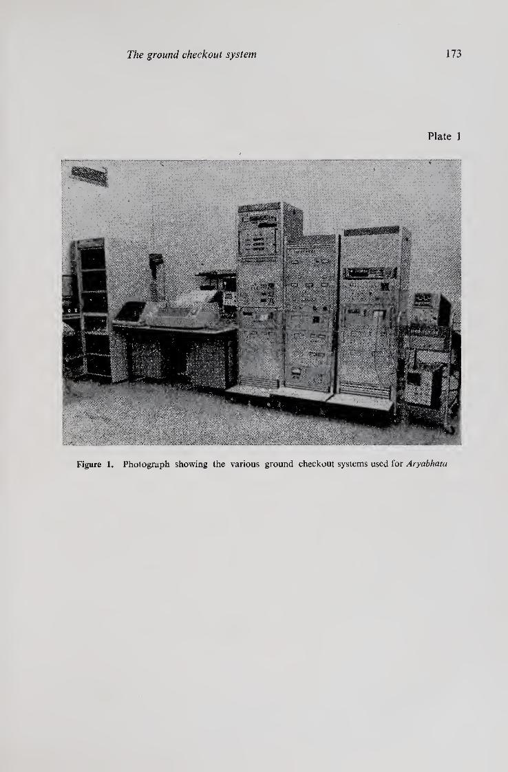
The ground checkout system 173
Plate 1
-
Figure 1. Photograph showing the various ground checkout systems used for Aryabhata

Orbit computations
R S BHAT and C K RAJASINGH ISRO Satellite Centre, Bangalore 560 058
MS received 8 July 1977; revised 2 December 1977
Abstract. Orbital information for Aryabhata was computed and made available for telemetry and tracking schedules and for mission analysis. Taking an available state- vector once in a week from USSR, the orbital computations were made for the first four months using a numerical integration procedure. During the later period of the mission, an analytical method was adopted to reduce the computer time. Aryabhata, in a near circular orbit at 600 km and having an inclination of 50.68°, experienced a constant atmospheric drag due to which the semi-major axis decayed by about 0-5 km in one year. The nodal regression rate, due to asphericity of the earth, was almost constant at 4-632°/day. The inclination remained constant throughout the year.
Keywords. Orbit; computation; satellite.
1. Introduction
Aryabhata, the first Indian satellite, was launched into a 600 km near-circular orbit at 50-68° inclination on 19 April 1975 by a Soviet rocket from Cosmodrome. Orbital information for Aryabhata was computed using the programs developed at ISRO Satellite Centre. The main objective of the orbit computations was to provide data for telemetry and tracking schedules and for mission analysis.
For the first four months, the satellite position and velocity vectors were computed accurately, by using a numerical procedure, based on an initial state-vector available (once in a week) from USSR. An analytical approach, for which prediction accuracy was lower but sufficient for telemetry and tracking schedules, was adopted later to reduce the computer time. Also the state-vectors were not available on a continuous basis after the first four months.
The limited tracking data available from SHAR could not be used for the refine¬ ment of orbital parameters as the orbit determination programme was not ready for operational use at that time. However, the Doppler data were used to adjust the absolute time (equatorial crossing time) and occasionally the right ascension of ascending node £2, during the later period when analytical procedure was adopted.
In both the programs only the effects due to the asphericity of the earth and at¬ mospheric drag are considered. It is assumed that all other perturbing forces cause negligible effects on the satellite’s motion. A brief description of the programmes and their performances is given here.
2. Orbital computations
The various external forces acting on a satellite may be classified into two groups,
•A list of symbols appears at the end of the paper
175

176 R S Bhat and C K Rajasingh
namely the central force and the perturbative forces. The central force is the gravi¬
tational force of a spherical earth which causes the spacecraft to move around the
earth in an elliptical path. The other forces like the atmospheric drag, asphericity
of the earth, luni-solar gravitational attraction, solar radiation pressure etc., consti¬
tute the perturbative forces. They are quite small in magnitude as compared to
central force. These forces influence the path of the satellite (in an elliptic orbit)
which is no longer a closed one (Escobal 1965; Herrick 1971). For close-earth
satellites, luni-solar perturbations and solar radiation pressure (leaving some special
cases) effects are several magnitudes less than those due to the asphericity of the
earth (Robertson 1968). In the analysis of the orbit of Aryabhata, only the effects
due to the asphericity of the earth and the atmospheric drag are considered.
2.1. Numerical method
The differential equations of motion with respect to a geocentric rotating co-ordinate
system (x pointing towards the Greenwich meridian, y perpendicular to x axis in the
equatorial plane and z axis pointing towards the north pole) including perturbing
forces are (El’yasberg et al 1974)
x = — - x + 2wey + wc2x — spvx + Ai*, r
y = y — 2a>ex -f a>e2y — spvy -f Aiy, r
z = — - z — spvz -f- AiA r
(1)
where s=CDA/2m; spvx, spvy and spvz are the perturbing acceleration components
due to the atmospheric drag; and Ai*, Aiy and A*z are the perturbing acceleration
components due to the asphericity of the earth.
The geopotential of the earth is given by
U = n/r+ Ud, (2)
where Ud is the disturbing potential given by
Ud = ~r [ ~ = 2 (t1)"7" P" (Sin ^ + (fL)2jP2’2 (sin ^
^^2,2 cos 2A -j- sin 2A^ (3)
An analytical model proposed by El’yasberg et al (1974) was used to compute the
atmospheric density, given by
p=PgK1K2K3Ki, (4)

Orbit computations 111
The differential equations of motion were integrated numerically by a 4th order Adams-Moulton predictor-corrector method to which the initial four values are supplied through a Runge-Kutta-Gill routine. Normally, computations of position and velocity vectors for a week with optimum step-size (40 s), took about 1-5 hr of computer time on an IBM 360/44. The optimum step-size was chosen after studying the behaviour of the time period with different step-sizes for about 50 revolutions. The behaviour is shown in figure 1. At the end of the week the predict¬ ed state-vector was compared with the current state-vector supplied by USSR. The difference was found to be of the order of 1 to 3 km in position and 1-3 s in the absolute time. One such example is presented in table 1.
2.2. Analytical method
As a first approximation for the satellite’s motion the Keplerian orbit is assumed. The orbit is represented by six parameters viz. the semi-major axis a, the eccentricity
Figure 1. Behaviour of the time period for 50 revolutions with different step-sizes.
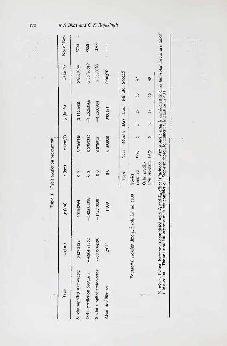
Tab
le
1.
Orb
it p
redic
tion p
rog
ram
me
178 R S Bhat and C K Rajasingh
> 0) u,
o Z
E J2 'w'
* N
e M
a M
& >v H
wo
co o CO oo VO oo
oo oo ON O
(N
o 6
s 0\ o o wo o VO
00 <N CO CN r** <N
CO
o
$ > I g s 00
■8
a 3 oo 3 > O
CO
§ 2? wo *
CN 1—H 00 o CN Os vo oo
VO vo w~. o vo CN o CN
I
O 6
os cs CO Os © wo CN Tf
CN vo CO
6 W) O u a a o
*s ;3 p
X) t-t O
co CN
o r- vo oo
CO On r- o o CN
'■b I
VO wo co wo
co CO 1—( vo Os os vo oo oo CO t"* l> 00 00 CO 00 00
© 6
o CO CO ©
(N
S wo
00 vb o oo
T T
U O 8 >
2 -8
> O
CO
o ■a
o o
o 6
os CO Os
CN CO © <N
a a o
8 a S
?§ *3
co
X) <
T3 a 8 0)
C/3
D a
Vh =3 o E
30 aj Q
a o
(-< aj <D !*
r- os Tf N-
vo vo wo wo
CN CN
vo os
wo
VO
ov
1 *3, &
13
8 oo wo
6 a a o
o >
cS
1 oo a
Ui a
+-> X u< O *
c3 a XT
w
Num
ber
of
zonal
har
mo
nic
s co
nsi
der
ed u
pto
/4
and J
M e
ffec
t is i
ncl
uded
. A
tmo
sph
eric
dra
g i
s co
nsi
der
ed an
d n
o l
uni-
sola
r fo
rces ar
e ta
ken
in
to a
cco
un
t.
The
sola
r ra
dia
tio
n p
ress
sure
is
not
con
sid
ered
. S
tep
-siz
e ch
ose
n f
or
nu
mer
ical
inte
gra
tion i
s 40
s.

Orbit computations 179
e, the inclination i, the argument of perigee a>, the right ascension of ascending node
£2 and the equatorial crossing time T. In due course, the variations in the orbital
parameters due to the perturbing forces are added. Only the secular effects due to
second zonal harmonic (J2) and the atmospheric drag are considered. No account
is taken of long and short periodic perturbations. The expressions for the varia¬
tions of orbital parameters are taken as given by King-Hele (1968), Sterne (1968)
and Robertson (1968). Due to the many approximations made in the orbit model,
the accuracy of the predictions was lower. At the end of the week, when the
predicted state-vector was compared with the current state-vector supplied by
USSR, the difference was found to be of the order of 50-100 km in position and
2-3 min in the absolute time. However, the accuracy was sufficient to keep the
telemetry and tracking schedules. The important advantage of this method is that
it takes only 10 min of IBM 360/44 time for predictions over a week’s period.
2.3. Computed orbital information
2.3a. Target designation
The information from onboard the satellite can be extracted by the ground station
when the satellite is above its horizon. The time spent by the satellite from horizon
to horizon is called visibility period. When h is greater than 0°, the satellite is
above the horizon of the station considered (figure 2). A control function to
check the visibility condition is
for visibility o < 90 cos a >0
_ (f-R)-R „ F = — —, > O
|r-R|
Figure 2. Geometrical representation of a satellite in a circular orbit around the earth for calculating the visibility period.

180 R S Bhat and C K Rajasingh
The satellite rises above the horizon of the station when CF changes sign from negative to positive, and sets when sign change is from positive to negative. Thus the visibility is determined.
During the visibility period, the position of the satellite in the topocentric co-ordinate system was determined by a co-ordinate transformation. The origin of the system is the ground station, and the axes are towards the local north, east and zenith directions. The position of the satellite with respect to the station is given by
Pt r G.
The co-ordinate transformation is accomplished as follows.
~ Pn~ sin 4>s cos 6 —sin <j>s sin 6 cos 4>s ~ Px
Pe = —sin 6 cos 6 0 Py
_Pz_ cos <f>s cos 6 cos 4>s sin 9 sin <f>s _Pz_
where 6 = 6g -f- Xs.
(6)
(7)
From the above transformation the azimuth and elevation are evaluated by
Az = tan“x (pM, h = sin"1 (j>JpT.
The range, azimuth and elevation history at 30 s interval during the visible portion of the orbit are called target designation and are used for orienting the tracking antenna in the direction of the satellite.
Aryabhata is visible to SHAR ground station four times a day. The maximum visibility period is about 13 min and the average visibility duration over a day is about 40-41 min.
2.3b. Eclipse characteristics
Since the power generated by the solar cells and the thermal condition of the onboard systems are dependent on the length of time the spacecraft spends in the sunlight, it is important to know this time. The time spent by the spacecraft in the earth’s shadow can be computed by knowing the position of the satellite and the sun. Stan¬ dard methods are available for determining the sun’s position. The earth shadow is assumed to be cylindrical as shown in figure 3. Depending on the position of the sun, the shadow period for Aryabhata varies from 0 to 37% of an orbit. For the first six months Aryabhata spent about 300 hr in sunlight. The eclipse characteristics of Aryabhata are shown in figure 4.
2.3c. Ground trace
Subsatellite point of a satellite is the pierce point of a ray dropped from the satellite in such a direction that it intersects normally the surface of the earth. The locus of
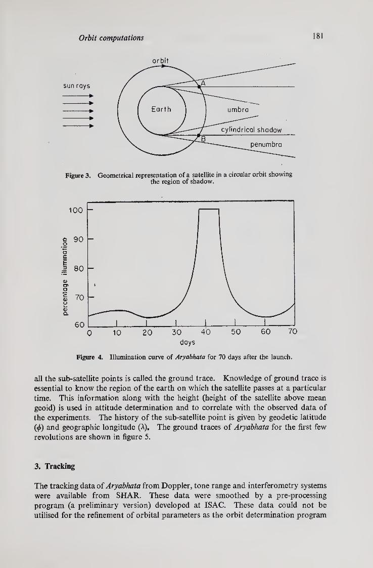
Orbit computations 181
sun rays
»•
*•
> >
Figure 3. Geometrical representation of a satellite in a circular orbit showing the region of shadow.
days
Figure 4. Illumination curve of Aryabhata for 70 days after the launch.
all the sub-satellite points is called the ground trace. Knowledge of ground trace is
essential to know the region of the earth on which the satellite passes at a particular
time. This information along with the height (height of the satellite above mean
geo id) is used in attitude determination and to correlate with the observed data of
the experiments. The history of the sub-satellite point is given by geodetic latitude
(<f>) and geographic longitude (A). The ground traces of Aryabhata for the first few
revolutions are shown in figure 5.
3. Tracking
The tracking data of Aryabhata from Doppler, tone range and interferometry systems
were available from SHAR. These data were smoothed by a pre-processing
program (a preliminary version) developed at ISAC. These data could not be
utilised for the refinement of orbital parameters as the orbit determination program

182 R S Bhat and C K Rajasingh
Figure 5. Ground trace of Aryabhata for the first 15 orbits after the launch.
was not ready for operational use at that time. However, the Doppler data were used to adjust the absolute time and occasionally the right ascension of ascending node ft. The observed minimum range, the calculated minimum range and the corresponding timings were compared and the differences were noted. The differ¬ ence in time is used to adjust the equatorial crossing time of the corresponding orbit. If too much difference is observed in the numerical values of the minimum range, the right ascension of node ft is adjusted by a geometrical procedure.
4. Performance of orbital predictions
The main objective of the orbital computations for Aryabhata was to cater to the needs of telemetry and tracking schedules for which the requirements of accuracy were relatively less stringent. In the initial phase of operations (first 4 months) the orbital predictions were generated using the state-vectors available from USSR. The predictions were accurate. However, for generating the complete orbital infor¬ mation the program used to take about 9-10 hr of computer time on an IBM 360/44 for a week. After 3 months of operation when the ground-trace information was suppressed, the program used to take about 3-4 hr of computer time.- For this reason the analytical model (with many approximations) was adopted later, even though the accuracy of orbit prediction was lower. Also the state-vector was not available on a continuous basis from USSR for the later period. Even the few

Orbit computations 183
Table 2 Orbital elements of Aryabhata
Orbit No. Semi-major axis
Eccentricity e
Inclination i (deg)
Right ascension of Node (deg)
Argument of perigee W (deg)
101 6967-781 0003150 50-707 233-018 39-083
201 6967-744 0-002918 50-686 191-849 84-702
301 6967-611 0-002730 50-684 160-791 113-587
401 6967-730 0-003087 50-693 129-828 131-769
501 6967-735 0-003057 50-682 98-787 148-358
601 6967-761 0003099 50-678 67-790 171-554 701 6967-673 0003235 50-674 36-779 197-995 801 6967-757 0-002820 50-681 5-774 221-239 901 6967-599 0-003481 50-671 334-765 241-277
1001 6967-636 0-003482 50-689 303-737 265-973
1101 6967-632 0002921 50-683 272-807 289-444 1201 6967-664 0-002991 50-686 241-720 318-314 1301 6967-742 0-002820 50-680 210-703 345-444 1401 6967-645 0-003131 50-678 179-687 16-196 1501 6967-705 0-002730 50-683 148-689 40-430
1601 6967-725 0-002881 50-676 117-680 66-205 1701 6967-662 0-002876 50-685 86-654 90-996 1801 6967-695 0-002932 50-688 55-309 120-286 1901 5967-624 0-02943 50-686 24-291 145-030 2001 6967-531 0003948 50-688 355-322 173-690
2101 6967-556 0-003943 50-688 323-278 198-249 2201 6967-493 0-003955 50-686 292-253 222-779 3500 6867-473 0-003395 50-695 248-454 173-160 5080 6967-353 0003427 50-688 118-782 196-135 5150 6967-327 0-003657 50-688 97-060 221-748
5500 6967-321 0-002286 50.689 348-540 305-452 5600 6967-254 0002849 50-687 317.508 329.887
state-vectors available were received late. However, the main objective of the mission, viz. to keep the telemetry and tracking sehedules, was successfully met. It was not possible to carry out a detailed orbital analysis for Aryabhata but the available state-vectors have been transformed to mean elements (short periodic perturbations subtracted) over a period of about one year, starting from orbit No. 101 to orbit No. 5600, to know the history of the orbit. Very little information is available after the 2000th orbit as seen from table 2. Hence, this result should be considered as tentative. The following observations can be made regarding the behaviour of the different orbital elements.
(i) The variation in the semi-major axis a over a period of about one year is shown in figure 6. The data points are approximated by a linear relation with time, show¬ ing that the semi-major axis for Aryabhata has decreased by about 0.5 km over one year duration. When the effect was evaluated by using a Jachia-65 atmospheric density model, the decay in a was found to be of the order of 1-25X 10~3 km/day.

184 R S Bhat and C K Rajasingh
100 200 300 lyear 400days
Figure 6. Approximate variation of the semi-major axis of Aryabhata as a function of time after the launch.
Hence the above decay in a was expected in the order of magnitude by theoretical estimation also.
(ii) The inclination i has almost remained constant (table 1) throughout the year with superimposed periodic variations of low amplitudes.
(iii) The eccentricity e and the argument of perigee show large periodic varia¬ tions. This may be due to the effect of asphericity of the earth, mainly due to the odd zonal harmonics.
(iv) The nodal regression rate (in right ascension of ascending node H) is found to be almost constant, having a value of the order of 4-632° per day as expected from theoretical calculations.
Conclusion
Orbit predictions of Aryabhata were carried out successfully and they met the main objective of the mission. Further improvements in the programs developed are in progress. When the orbit determination program becomes operational it is hoped to carry out a detailed orbit analysis of Aryabhata with the available tracking data. However, the orbital information generated was useful in calculating the solar-array voltages, temperature conditions of the spacecraft etc.
Acknowledgements
We are grateful to Prof. U R Rao and Dr A S Prakasarao for their encouragement and fruitful suggestions throughout the period of this work.

Orbit computations 185
List of symbols
A
Az
cD CF
Q,2> ^2,2 G
projected area of the satellite azimuth drag coefficient of the satellite control function for visibility second order tesseral harmonic coefficients of the earth station vector with reference to geocentric inertial co-ordinate
h
^min Jn
system elevation of the satellite above the ground station minimum elevation of the antenna (for Aryabhata hmjn = 0) zonal harmonic coefficients of the earth of nth order
Kv K2, K3, factors describing change in atmospheric density due to respectively (1) solar radiation intensity F, relative to some average level
m
Pn (sin <f>), ■) F2)2 (sin </>) ) Re
r
r s
U
Ud V
x, y, z
intensity F0; (2) diurnal effect; (3) semi-annual effect and (4) geomagnetic perturbation mass of the satellite
Legendre polynomials
mean equatorial radius of the earth radial displacement of the satellite from geocentre radius vector of the satellite geocenrtic inertial co-ordinate system ballistic parameter of the satellite (5 = CDA/2m) geopotential of the earth disturbing potential due to asphericity of the earth velocity of the satellite components of the radius vector with respect to the geocentric co¬ ordinate system
x,y, z components of the velocity vector in geocentric rotating co-ordi¬ nate system
x, y, z components of the acceleration vector in the geocentric co-ordinate system
z e
o9 KK
F P
Ph
PT> Px> Py, Pz
unit vector along the zenith of the station local sidereal angle of the station (9 — 6g + As) sidereal angle of the Greenwich meridian geographic longitude of the satellite and station gravitational constant of the earth atmospheric density night time vertical profile of the atmospheric density range components of the range vector in geocentric inertial co-ordinate system
Pn> Pe> Pz components of the range vector in topocentric horizontal co¬ ordinate system geodetic latitude of the satellite and station respectively sidereal rate of the earth

186 R S Bhat and C K Rajasingh
References
Allione M S 1968 The A-body problem and special perturbation techniques; guidance, flight mecha¬ nics and trajectory optimisation Vol. VI NASA-CR-1005
El’yasberg P E, Kuganento B V and Sinitrsyn V N1974 Algorithms for the computation of navigation information about the position of the satellite (Russian) USSR Academy of Sciences, Moscow
Escobal P R 1965 Methods of orbit determination (New York: John Wiley) Gaposchkin E M 1964 Differential orbit improvement (DOI-3) SAO Spl. Rep. No. 161 Herric S 1971 Astrodynamics Vols. I and II (London: Van Nostrand) Sterne T E 1968 in General perturbation theory; guidance, flight mechanics and trajectory optimisation
ed. B Kampos NASA CR-1008 Kampos B 1968 General perturbation theory; guidance, flight mechanics and trajectory optimisation
NASA-CR-1008 King-Hele D G 1914 Theory of satellite orbits in an atmosphere (London; Butterworth) Jenson J, Kork J, Kraft D and Townserd G 1962 Design guide to orbital flight (New York:
McGraw Hill) Lalbowe A G 1964 High accuracy orbit prediction from node to node. Astronaut. Acta 253
Me Cuskey 1963 Introduction to celestial mechanics (Melno Californea: Addison-Wesley) Robertson R L 1968 Mission constraints and trajectory interfaces. NASA CR-1015 Walter H G and Scafer M K 1966 Determination of the position of the sun on the basis of the mean
solar elements. ESRO SN-10 Walter H G and Wales I M 1967 The differential correction of close earth satellite orbits. ESRO
SR-7 Wolverton R W 1963 Handbook of orbital operations (New York: John Wiley)
A statistical analysis of weight and cost parameters of spacecraft with special reference to 4 Aryabhata ’
P N PATHAK ISRO Satellite Centre, Peenya, Bangalore 560 058
Present Address: Remote Sensing Area, Space Applications Centre (ISRO), Ahmedabad 380 053
MS received 16 April 1977; revised 28 July 1978
Abstract. The available data on the weights of several NASA and ESRO spacecraft have been statistically analysed using the regression analysis technique and empirical relationships of the type WT — AfVx& have been established, where WT is the total weight of the spacecraft, Wx is the weight of one of its chosen subsystems and A and /? are constants for the chosen subsystem. It is found that the weight data of Aryabhata show a fairly good fit with these empirical relationships. Further, using an established statistically derived relationship for NASA satellites, involving the cost of a space¬ craft and its weight parameters, it is found that the cost of Aryabhata is much lower than that of other NASA satellites of comparable weight. The implications of these results are briefly discussed.
Keywords. Spacecraft weight; spacecraft cost.
1. Introduction
The weight and cost of a spacecraft are two important parameters on which careful control needs to be exercised. Whereas the shape and size of a spacecraft are essen¬ tially dictated by the shroud of the launch vehicle, the allowable total weight of space¬ craft is limited by the capability of the launch vehicle. A few studies (Dondi 1971 and references therein; Clemens et al 1973) have indicated that the cost of a spacecraft can be expressed as a function of its weight and other technical parameters. Here we have analysed the available data (Dondi 1971) on the weight and cost of several spacecraft and compared the results with the corresponding data of Aryabhata.
The following statistical analyses have been made,
(i) The available data on the weight parameters of different NASA and ESRO (European Space Research Organisation, now ESA, European Space Agency) satellites (Dondi 1971) have been used in regression analyses and the results are compared with the weight data of Aryabhata.
(ii) Based on an established empirical relationship between the cost of a space¬ craft and its weight parameters, a comparison has been made between the cost of Aryabhata and the costs of several NASA satellites of comparable weight but having diverse complexities and mission goals.
A list of symbols appears at the end of the paper.
187
P.(C)-5
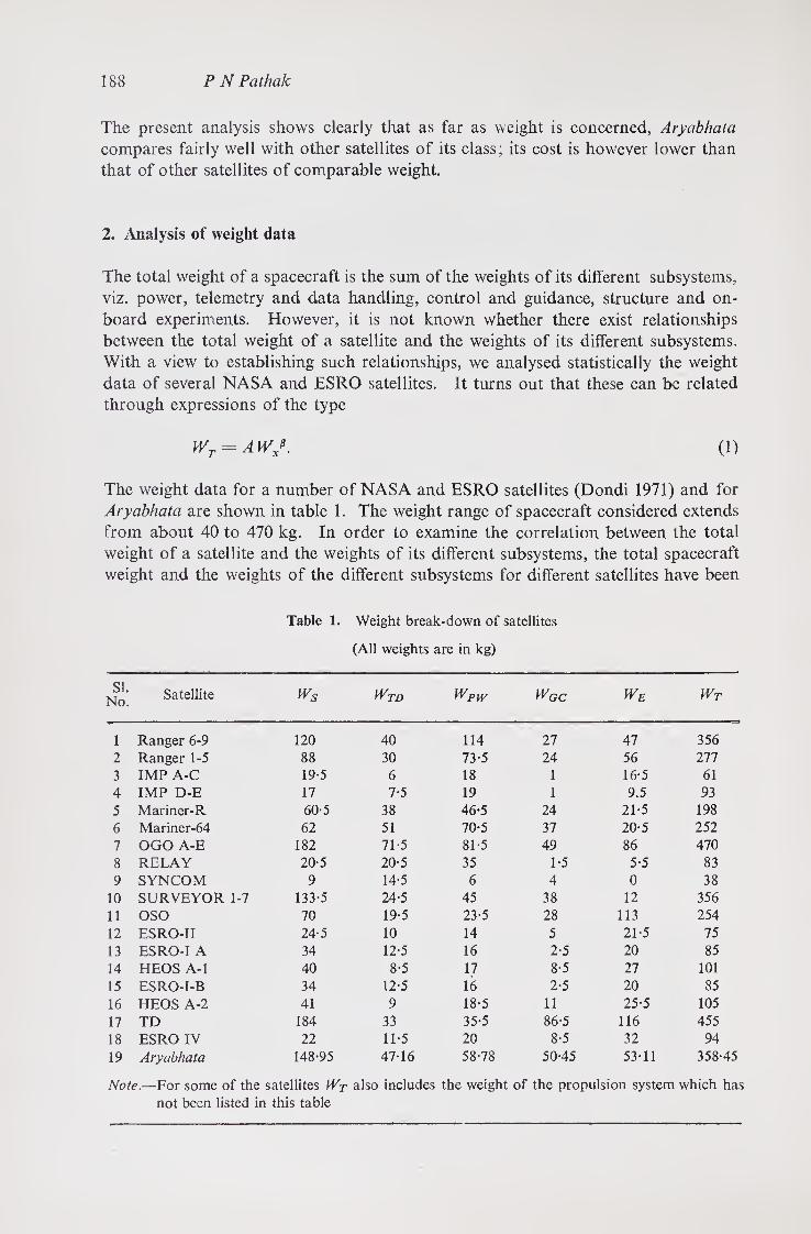
188 P N Pathak
The present analysis shows clearly that as far as weight is concerned, Aryabhata
compares fairly well with other satellites of its class; its cost is however lower than that of other satellites of comparable weight.
2. Analysis of weight data
The total weight of a spacecraft is the sum of the weights of its different subsystems, viz. power, telemetry and data handling, control and guidance, structure and on¬ board experiments. However, it is not known whether there exist relationships between the total weight of a satellite and the weights of its different subsystems. With a view to establishing such relationships, we analysed statistically the weight data of several NASA and ESRO satellites. It turns out that these can be related through expressions of the type
WT = A WJ. (1)
The weight data for a number of NASA and ESRO satellites (Dondi 1971) and for Aryabhata are shown in table 1. The weight range of spacecraft considered extends from about 40 to 470 kg. In order to examine the correlation between the total weight of a satellite and the weights of its different subsystems, the total spacecraft weight and the weights of the different subsystems for different satellites have been
Table 1. Weight break-down of satellites
(All weights are in kg)
51. No. Satellite WS WTD WPW Wgc WE WT
1 Ranger 6-9 120 40 114 27 47 356 2 Ranger 1-5 88 30 73-5 24 56 277 3 IMP A-C 19-5 6 18 1 16-5 61 4 IMP D-E 17 7-5 19 1 9.5 93 5 Mariner-R 60-5 38 46-5 24 21-5 198
6 Mariner-64 62 51 70-5 37 20-5 252
7 OGO A-E 182 71-5 81-5 49 86 470
8 RELAY 20-5 20-5 35 1-5 5-5 83 9 SYNCOM 9 14-5 6 4 0 38
10 SURVEYOR 1-7 133-5 24-5 45 38 12 356
11 OSO 70 19-5 23-5 28 113 254 12 ESRO-II 24-5 10 14 5 21-5 75
13 ESRO-I A 34 12-5 16 2-5 20 85
14 HEOS A-l 40 8-5 17 8-5 27 101
15 ESRO-I-B 34 12-5 16 2-5 20 85
16 HEOS A-2 41 9 18-5 11 25-5 105
17 TD 184 33 35-5 86-5 116 455
18 ESRO IV 22 11-5 20 8-5 32 94
19 Aryabhata 148-95 47-16 58-78 50-45 53-11 358-45
Note.—For some of the satellites Wj also includes the weight of the propulsion system which has not been listed in this table

at 1st i
500
400
300
200
1 00
0
100
60
20
30
10
ioo'
60
20
80
40
0
100
60
20
al analysis of weight and cost parameters of spacecraft
.1—1..I I .1 J 1 J .1..1 1-L. I—L
i id 3 U W
I I - w <t O j a) r ^ cl o. 3 § 2 5
I
<D 05 C C o >- 8
e> -2 c o e
o >N
o I o a:
S 1 CD <j B
o U_ V—'
^^cocoljcoujOco tfiOuiuiujihuj
O co a: o
CM l
< CO o
a O C/5
*5 *3 d s * o « O 43 <D x a
& o x\ o X
<D £ 53 cd S-4 co bo <D c3 X
.22 'S
2 8 T3 a> « to
Q. <D TTX 0) -♦_*
<D e C3 a
00 « *—I 4-3
£ ^ ,0 a) C*-i - 00
&> Q
X) G cd w ^ 4- a a
T3 d> <D to -4-* M—I </5 .-H
vS ° _* C/5 C3 -*->
it ~ y 43 ? £P n-t
1 O !> c3 <U
£
§
a> X
189

190 P N Pathak
Figure 2. Scatter plot of log Wt against log Ws. The data point corresponding to Aryabhata is shown in the diagram by a star.
Table 2. Correlation co-efficients between different variables
Variables Correlation coefficients
log WT, log Ws 0-96 ± 0-02
log Wt, log Wjd 0-81 ± 0-08 log Wt, log Wpty 0-85 ± 0 06
log WT, log WE 0-63 ± 0-15
log WT, log Wgc 0-80 ± 0 06
Table 3. Coefficient A and exponent jS in equation (1)
Subsystem A P
Structure 5-69 0-85 Telemetry and data handling 12.2 0-86 Power 8.3 0-86 Experiments 27-1 0-53 Guidance and control 491 0-49
plotted in figure 1. It can be seen from this figure that the weights of different sub¬ systems show good correlation with the total weight of the spacecraft.
Figures 2-6 show the scatter plots of log WT against log Wx (where x stands for different subsystems). In table 2, the correlation coefficients corresponding to these scatter plots are given. Note that all the correlation coefficients are high and
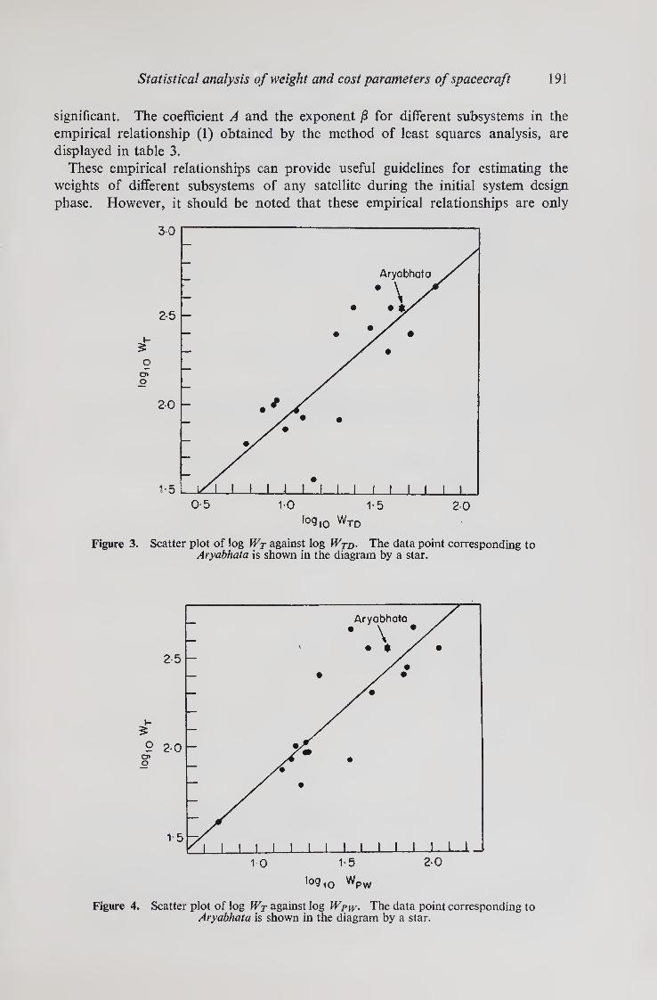
Statistical analysis of weight and cost parameters of spacecraft 191
significant. The coefficient A and the exponent jS for different subsystems in the
empirical relationship (1) obtained by the method of least squares analysis, are
displayed in table 3.
These empirical relationships can provide useful guidelines for estimating the
weights of different subsystems of any satellite during the initial system design
phase. However, it should be noted that these empirical relationships are only
Figure 3. Scatter plot of log WT against log Wjd- The data point corresponding to Aryabhata is shown in the diagram by a star.
10 1-5 20
log,0 Wpw
Figure 4. Scatter plot of log Wy against log Wpw. The data point corresponding to Aryabhata is shown in the diagram by a star.
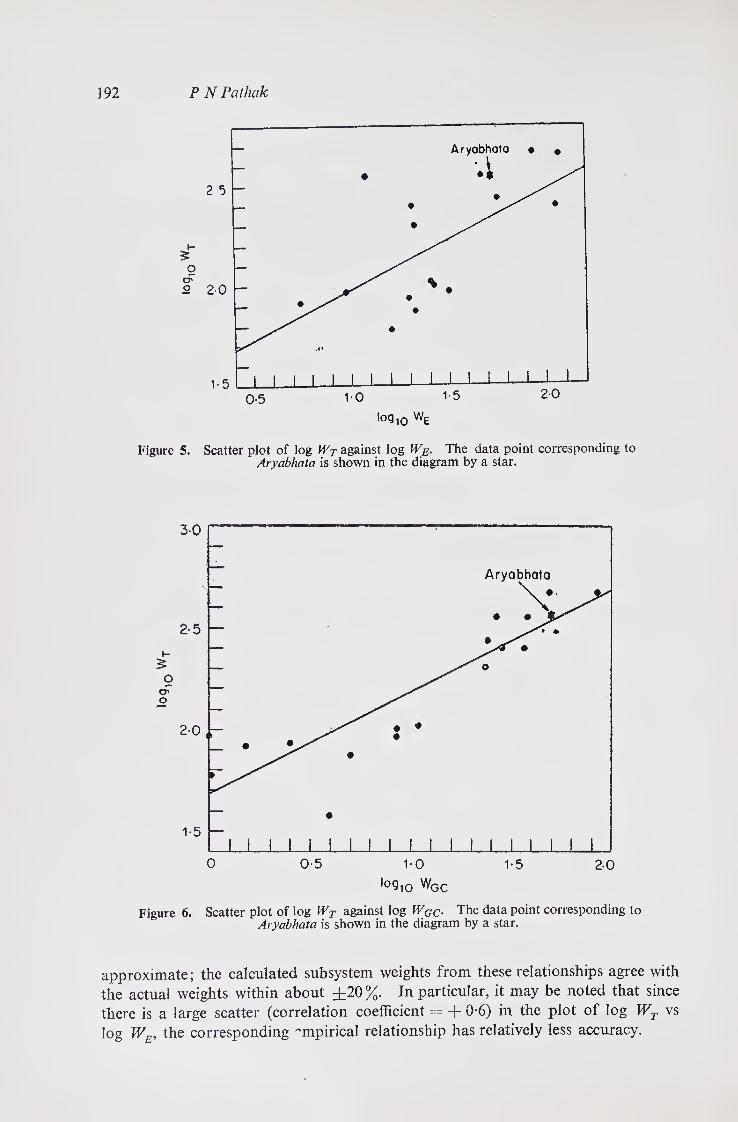
192 P N Palhak
Figure 5. Scatter plot of log WT against log IVE. The data point corresponding to Aryabhata is shown in the diagram by a star.
Figure 6. Scatter plot of log WT against log WGC. The data point corresponding to Aryabhata is shown in the diagram by a star.
approximate; the calculated subsystem weights from these relationships agree with
the actual weights within about ±20 %. In particular, it may be noted that since
there is a large scatter (correlation coefficient = -f 0-6) in the plot of log WT vs
log WE, the corresponding empirical relationship has relatively less accuracy.

Statistical analysis of weight and cost parameters of spacecraft 193
It is important to note that weight data for different subsystems of Aryabhata
show a fairly good fit with these empirical relationships, as may be seen from the
scatter plots (figures 2-6).
It is important to note here that in deriving these relationships we have used the
weight data of different NASA/ESRO satellites of the late sixties. It seems quite
possible that with advancement in satellite technology, these weight relationships
might change.* It would be therefore important to also study such weight relation¬
ships for the satellites of 1970’s which represent a higher level of technology than that
for the earlier period. In this context it is significant to note that these weight rela¬
tionships when applied to the recent satellites of ISRO, viz. APPLE and INSAT,
give consistently underestimated values for the total in-orbit weights for these satel¬
lites.
3. Relationship between weight and cost of spacecraft
Some studies (Dondi 1971 and references therein; Clemens et al 1973) have been
made to establish empirical relationships between the cost of a spacecraft and its
different weight parameters. For example, the total cost CSG of a spacecraft
including the cost of experiments and cost of the relative ground support (i.e.
launch vehicle and mission support) is given by the Goddard formula
CSG = 25-95 (WTDf WT)V237 • (TV WT)V0S • (DTC. TAR)0 035 Rs. in lakhs (2)
where the cost is in lakhs of rupees, and we have taken $ 1 =Rs. 7-50. Note that
in the above formula, the cost is strongly dependent upon (i) the complexity
factor for the satellite (WTJWT) i.e., the ratio of the weight of the telemetry and
data handling subsystem to the total weight of the satellite and (ii) NWT — i.e., the
total weight of the manufactured satellites v/ith the package of on-board experi¬
ments (prototype and flight models). The last factor in equation (2) which involves
the product of the ‘degree of time compression’ and ‘technical advance required’
does not contribute significantly to the total cost.
For comparison with Aryabhata, we use the following values for the different
parameters:
TV — 3 (prototype and two flight models); DTC = 4; and TAR = 3.
Using the empirical relationship between WT and WTD as established in § 2,
equation (2) can now be simplified to:
CSG = 2-54 WTV28 Rs. in lakhs. (3)
We shall call (3) the modified Goddard formula. This equation has been plotted
in figure 7 along with the cost data (Dondi 1971) of some NASA satellites (3 models
for each) and of Aryabhata. The total cost of Aryabhata has been derived as follows.
The total cost of the three models of Aryabhata is Rs. 3-5 crores. Adding to this
Rs. 1-5 crores for the approximate cost for the subsystems (spin system., chemical
battery, solar panels and tape recorders) supplied by the USSR Academy of Sciences,
*The author is thankful to the referee for this suggestion.

194 P N Pathak
Figure 7. The cost of spacecraft as a function of its total weight as given by the modified Goddard formula (equation (3)). The cost data of several NASA satellites and of Aryabhata are also shown.
which is considered a reasonable estimate in view of the international cost of these
items, the total cost of Aryabhata works out to be Rs. 5 crores. However, this cost can¬
not be directly compared with the costs of NASA satellites (shown in figure 7) which
include the cost of the relative ground support also. From the cost data of NASA
satellite projects (Dondi 1971) it is found that, on an average, the cost of a spacecraft
including on-board experiments works out to be about 60% of the total cost, while
the remaining 40% accounts for the relative ground support. Thus, based on this
result and using (3), the cost of a spacecraft including on-board experiments, for a
satellite of the same weight as that of Aryabhata (i.e. 350 kg), works out to be about
Rs. 27 crores, which is about five times higher than the cost of Aryabhata.
4. Discussion of results
The result regarding the cost aspect of Aryabhata is quite significant and therefore,
this warrants a more detailed study by taking into consideration the data regarding

Statistical analysis of weight and cost parameters of spacecraft 195
the cost, weight as well as other technical factors related to the complexity of a satel¬
lite. Although the complexity factor WTD/WT is hidden in the modified Goddard
formula (equation (3)) it does not seem to be applicable to Aryabhata. This might
mean that probably the factor WTD/WT may not be a true representation of the com¬
plexity of Aryabhata. Alternatively, other technical parameters related to spacecraft
capability such as available power, type of stabilisation and control system, number of
experiments, telemetry bit rate etc. of a spacecraft should also be considered for the
analysis of cost estimation. In this connection it is important to note that from the
consideration of the available power*, Aryabhata does not compare well with the
NASA satellites of similar weight. Whereas Aryabhata's, available power is 46 W,
the average power level for NASA satellites of 400 kg weight is about 200 W.
Perhaps this could be one of the possible reasons for the lower cost of Aryabhata.
However, this should be considered tentative until it is verified by rigorous analysis.
In this context it would be more meaningful to study Aryabhata's weight versus capa¬
bility in relation to other satellites.
In addition, there could also be some nontechnical reasons for the lower cost of
Aryabhata, and prima facie the following two causes appear to be more significant.
(i) The lower overhead charges and salary structure in India as compared to
those in USA.
(ii) The practice of sub-contracting normally followed in NASA satellite pro¬
grammes might involve larger costs compared to in-house activities as was the
case with Aryabhata.
5. Conclusions
The main conclusions that can be drawn from the present analysis are summarised
as follows.
(i) The statistical analysis of the weight data of several NASA and ESRO satel¬
lites does indicate empirical relationships between the total weight of a space¬
craft and the weight of any of its subsystems. These empirical relationships
can provide useful guidelines during the initial system design phase of a space¬
craft.
(ii) The existing Goddard formula for estimating the cost of a spacecraft has been
simplified so that the cost is given as a function of only the total weight of the
spacecraft.
(iii) Based on the empirical relationships mentioned in (i) and (ii) above, a com-
paiison of the weight and cost parameters of Aryabhata shows that whereas
the subsystem weight parameters of Aryabhata are in good agreement with
those of other satellites of comparable weight (i.e. about 350 kg), the cost of
Aryabhata is much lower than the cost of other satellites of similar weight.
In view of the ongoing and future satellite programmes of ISRO, it would be
worthwhile to compare the costs of several Indian satellites with those of NASA
and ESRO satellites, along with other relevant parameters. It might turn out
from this analysis that such direct comparisons are not justified. A somewhat
*The author is thankful to the referee for pointing out this.
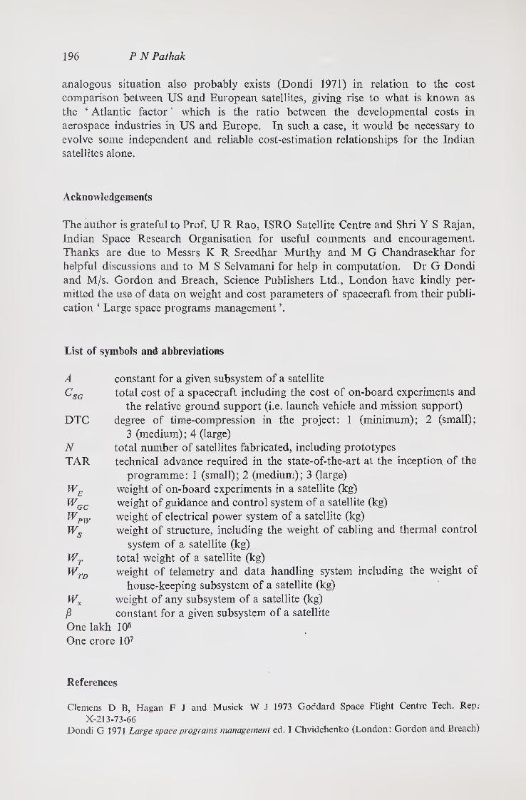
196 P N Pathak
analogous situation also probably exists (Dondi 1971) in relation to the cost
comparison between US and European satellites, giving rise to what is known as
the ‘ Atlantic factor ’ which is the ratio between the developmental costs in
aerospace industries in US and Europe. In such a case, it would be necessary to
evolve some independent and reliable cost-estimation relationships for the Indian
satellites alone.
Acknowledgements
The author is grateful to Prof. U R Rao, ISRO Satellite Centre and Shri Y S Rajan,
Indian Space Research Organisation for useful comments and encouragement.
Thanks are due to Messrs K R Sreedhar Murthy and M G Chandrasekhar for
helpful discussions and to M S Selvamani for help in computation. Dr G Dondi
and M/s. Gordon and Breach, Science Publishers Ltd., London have kindly per¬
mitted the use of data on weight and cost parameters of spacecraft from their publi¬
cation ‘ Large space programs management ’.
List of symbols and abbreviations
A constant for a given subsystem of a satellite
CSG total cost of a spacecraft including the cost of on-board experiments and
the relative ground support (i.e. launch vehicle and mission support)
DTC degree of time-compression in the project: 1 (minimum); 2 (small);
3 (medium); 4 (large)
N total number of satellites fabricated, including prototypes
TAR technical advance required in the state-of-the-art at the inception of the
programme: 1 (small); 2 (medium); 3 (large)
WE weight of on-board experiments in a satellite (kg)
WGC weight of guidance and control system of a satellite (kg)
Wpw weight of electrical power system of a satellite (kg)
Ws weight of structure, including the weight of cabling and thermal control
system of a satellite (kg)
WT total weight of a satellite (kg) WTD weight of telemetry and data handling system including the weight of
house-keeping subsystem of a satellite (kg)
Wx weight of any subsystem of a satellite (kg)
j8 constant for a given subsystem of a satellite
One lakh 105
One crore 107
References
Clemens D B, Hagan F J and Musick W J 1973 Goddard Space Flight Centre Tech. Rep.
X-213-73-66 Dondi G 1971 Large space programs management ed. I Chvidchenko (London: Gordon and Bi'each)

Aii experiment to detect energetic neutrons and gamma rays from the sun
M V K APPA RAO, S V DAMLE, R R DANIEL, G S GOKHALE, GEORGE JOSEPH, R U KUNDAPURKAR and P J LAVAKARE Tata Institute of Fundamental Research, Colaba, Bombay 400 005
MS received 16 April 1977; revised 5 December 1977
Abstract. A payload for the detection and measurement of high energy neutrons and gamma rays from the sun was flown onboard the first Indian satellite Aryabhata. The payload system for this neutron-gamma experiment was designed for detecting energetic neutrons in the energy range 10-500 MeV and gamma rays in the energy range 0-2-20 MeV. The details of the design of the payload, various tests carried out on it as well as the preliminary in-orbit performance are presented.
Keywords. Satellite instrumentation; solar neutron experiment.
1. Introduction
The emission at times of solar flares of a variety of combinations of electromagnetic radiations from radio through gamma rays, and of energetic charged particles, is now well established. In addition, it is certainly to be expected that nuclear reactions induced by energetic charged flare particles on the solar surface could take place, giving rise to neutrons and gamma rays. Indeed, during the August 1972 flare, Chupp et al (1973) from instruments on OSO-7, have observed intense nuclear gamma ray line emission in addition to the continuum. However, so far there is no well- established evidence for high energy neutron emission during times of intense solar activity. While the emitted charged particles would be affected by the interplanetary magnetic field, the neutral radiation viz., neutrons and gamma rays, can directly reach the earth; thus observations on them could provide a new method of studying the solar flare phenomenon. Though most of the low energy neutrons (<10 MeV) would decay during the sun-earth journey, the energetic ones have a reasonable chance of reaching the earth. Also, the simultaneous observations of neutrons and gamma rays in a single event would be able to establish reliably the generic relation between them. With this primary objective we designed an experiment in which the technique of pulse shape discrimination in a scintillator crystal was employed to separate neutron events from gamma ray events. This technique proven by us in balloon experiments (Daniel et al 1970; Joseph 1970) was used in the design of an experiment in the first Indian scientific satellite Aryabhata. In this paper we describe the scientific objectives of this experiment and the various technical aspects including the performance of the payload during the environmental qualifying tests, and during tests carried out after the integration of the payload with the satellite—namely, the
197
198 M V K Appa Rao et al
autonomous and complex tests carried out at Bangalore, India, and at the USSR Cosmodrome. The performance of the payload in orbit, based on preliminary analysis of the limited data obtained during the first few orbits, is also described.
2. Scientific objectives
The experiment was designed with the following scientific objectives.
(i) To detect simultaneously the possible impulsive emission of energetic neutrons (10-500 MeV) and gamma rays (0-2-20 MeV) at times of intense solar activity. The possibility of observing the delayed signal from neutrons with respect to gamma rays is an important capability of the experiment.
(ii) To detect any steady or quasi-steady solar emission of energetic neutrons and gamma rays.
(iii) To measure the splash albedo flux of neutrons and gamma rays as a function of latitude.
(iv) To detect gamma ray bursts of the type first discovered by Vela satellites and any other type so far not discovered.
3. Design of the experiment and fabrication of the payload
3.1. Design of the experiment
The principle of the detection and separation of neutrons and gamma rays is based on the fact that in an inorganic crystal scintillator like CsI(Tl), the high rate of ionisation (dE/dx) due to the low energy protons and helium nuclei released in nuclear inter¬ actions caused by neutrons, gives rise to a pulse shape different from the low (dE/dx)
due to the fast electrons originating from gamma ray interactions in the crystal (Mathe and Schlenk 1964). Specifically, the derivative of these two pulse shapes would cross the zero axis at different points—earlier for neutrons and a little later for gamma rays. This cross-over time (T) is characteristic of the rate of energy loss and is independent of the amplitude of the pulse. Taking advantage of this property, we can separate the two types of events and measure the energy deposited in the crystal, event by event. This unique capability is potentially useful for detecting even small increases in the neutron flux.
In order to ensure that the relatively over-abundant low energy gamma ray flux is recorded with a minimal efficiency without appreciably reducing that of neutron detection, a large area small thickness disc of CsI(Tl) crystal of 12-5 cm diameter and 1-27 cm thickness, was chosen as the basic detector. The pulse shape discrimination (PSD) technique separates neutron and gamma ray events which deposit more than 4 MeV in the crystal. However, for gamma rays with E <4 MeV, the PSD technique is not required and the detector samples them purely on the basis of energy release in three suitable energy bins between 0-2 and 4 MeV. The experiment makes a two- dimensional analysis, for E (> 4 MeV) and T, each analysed in 64 channels.
The minimum detectable solar flux for neutrons is estimated to be 5 X 1(P3

Eenergetic neutrons and gamma rays from the sun 199
neutrons/cm2 s, while the minimum detectable flux of gamma rays is & 10~2 photons/cm2 s. However, in order to arrive at reliable absolute fluxes, it will be advisable to calibrate the instrument using neutron and gamma ray beams of known energy from accelerators. Mention may also be made that charged particles which cause a coincidence between the 4n anticoincidence shield and the main detector (COIN) were also continuously monitored.
3.2. Payload construction details
The experimental payload consisted of two boxes, hereafter referred to as Ex-21 and Ex-22. The physical dimensions for Ex-21 and Ex-22 were 278 mm X 245 mmx 245 mm, and 278 mmx245 mmx 140mm respectively. The weights were 15\2 kg and 4-7 kg respectively. The two packages were placed one above the other, with Ex-21 near the deck plate, in bay No. 7 of the belly-band of the satellite as shown in figure 1.
The main detector crystal housed in Ex-21 was viewed by a 12-5 cm diameter photo¬ multiplier tube and completely surrounded by a 1 cm thick NE-102 plastic scintillator viewed by four 3-81 cm diameter photomultiplier tubes; the latter served as the charged particle anticoincidence shield for the main detector. The pulse amplifiers for the CsI(Tl) and plastic scintillator, the PSD logic electronics and the high voltage supply for the photomultipliers were housed at the back of Ex-21. At the front end
-x
TIFR equipment lay-out on deck plate
approx, scale : 1:15
Figure 1. A schematic diagram showing the position of the experiment in the satellite.
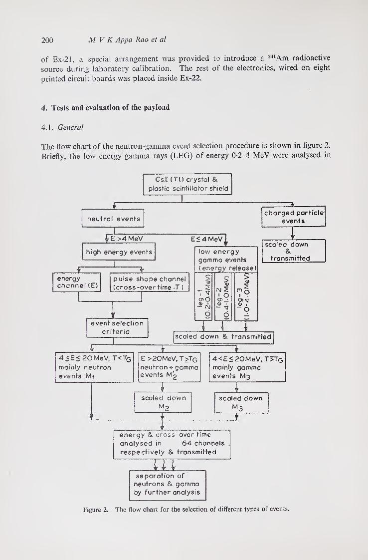
200 M V K Appa Rao et al
of Ex-21, a special arrangement was provided to introduce a 24lAm radioactive source during laboratory calibration. The rest of the electronics, wired on eight printed circuit boards was placed inside Ex-22.
4. Tests and evaluation of the payload
4.1. General
The flow chart of the neutron-gamma event selection procedure is shown in figure 2. Briefly, the low energy gamma rays (LEG) of energy 0-2-4 MeV were analysed in
Csl (TU crystal & plastic scintillator shield
_L neutral events
charged particle events
E >4 MeV E<4 MeV
high energy events
energy channel (E)
pulse shape channel (cross-overtime T )
event selection criteria
low energy gamma events (energy release)
> <B
tI CT>0 Q} * ~ CM
* (\j2
- ^r
m
> <t> 2
0)^1 <D i
scaled down &
transmitted
scaled down & transmitted
£ 4 <E< 20MeV, T<TG mainly neutron events
£ E >20 MeV, T>TG neutron + gamma events M->
i
1 4 <E < 20MeV, T>TG mainly gammo events M3
scaled down M p
1. scaled down
m3
ZZJ-
energy & cross-over time analysed in 64 channels respectively & transmitted
separation of neutrons & gamma by further analysis
Figure 2. The flow chart for the selection of different types of events.

Energetic neutrons and gamma rays from the sun 201
three energy bins without recourse to PSD, while the events giving energy loss > 4MeV were analysed on the basis of their pulse shape, using the PSD technique. Since the telemetry readout is made every second, the various types of events were sampled suitably depending on the calculated counting rates in orbit and shown in table 1. To set various thresholds in terms of energy released in the CsI(Tl) crystal, 5-49 MeV alpha particles from the M1Am radioactive source were used.
For the plastic scintillator, the threshold was set using the observed pulse height for 279 keV gamma rays from the radioactive source 203Hg. Further, the rejection efficiency of the anticoincidence shield was checked using cosmic ray mu-mesons.
4.2. Bench tests
After setting various thresholds as described in § 4T above, the electronic logic was thoroughly checked, and the boxes Ex-21 and Ex-22 were integrated to carry out further tests. All the information on the eight parameters of the experiment, namely, LEG-1, LEG-2, LEG-3, COIN, E, T and indicators Ml and M3, were available as 35 parallel bits when the telemetry interrogation pulse entered the experiment. For the bench test, a special test unit—the digital data interface unit (DDIU)—was built. This unit scans the experiment every one second, accepts 35 parallel bits, decodes the information and prints the data for the eight experimental parameters on a HP505OB printer.
First, 549 MeV alpha particles from the 241Am radioactive source were used to simulate neutron-like events. Next, the background gamma ray data which provides information on LEG-1, LEG-2, LEG-3, COIN and the E, Tplot for Ml and M3
type events were taken. This gave very good separation between neutron-like and gamma ray events. After thoroughly testing the experiment on the bench it was
Table 1. Expected and observed counting rates for the neutron-gamma experiment
Types of events Expected
Minimum Maximum (counts/s) (counts/s)
Observed in orbit 2 from SHAR (Preliminary)
(counts/s)
1. Low energy LEG-1 15 90 17 gamma ray (0-2-0-4 MeV) events (energy T FG-2
12 release) (0-4-1-0 MeV) 72 14
LEG-3 (1-4 MeV) 7 42 8
2. High energy gamma ray
4-20 MeV 2 12 not determined
events (energy release)
> 20 MeV 0-5 3 yet
3. High energy gamma ray events (energy releasej
neutron events 0-01 0-2 0-05
4. Charged particles
coincidence events 30 200 31

202 M V K Appa Rao et al
integrated with the satellite and the environmental, autonomous and complex tests described below were carried out.
4.3. Environmental tests
After thoroughly testing the experiment in the laboratory, the payload was subjected to the following environmental tests:
temperature cycling (—10°C to -f-55°C), thermovac tests (temperature cycling in the range — 10°C to -j-55°C and
vacuum level of 10-6 mm of mercury), shock and vibration tests at specified levels.
The intercomparison of the data obtained during these tests and the bench tests showed that the variation of parameters was within the acceptable limits.
After full qualification of the payload in the environmental tests, it was again thoroughly checked in the laboratory before integrating it with the satellite.
4.4. Autonomous test
After integration of all the experiments with the satellite, the autonomous test in which only the neutron-gamma experiment was powered, was performed in two stages. In the first stage, the experimental packages were placed in the satellite and the experiment was powered through the satellite power system. Using the DDIU, 211 Am calibration data and the background data were taken. In the second stage, with experimental packages in the same position, the data were taken through the satellite telemetry system and the data decoded and printed out using an on-line PDP-11 computer. The data compared very well with the bench test data.
4.5. The complex test
In this test all the subsystems of the satellite were integrated and the data taken through satellite telemetry when all the subsystems were powered. The data were taken in similar fashion as in the second stage of the autonomous tests. The data compared well with autonomous test results indicating that there was minimum of interference from other subsystems, and that the experiment was working satis¬ factorily in this mode. Further, complex tests were performed with the solar panels in position. Again, the data showed that the experiment was working satisfactorily.
4.6. Autonomous and complex tests at the Cosmodrome
After thoroughly testing the experiment as described above, the integrated satellite was taken to the Cosmodrome in the USSR. Autonomous and complex tests in various modes were carried out. The data showed that the experiment was working satisfactorily.

Energetic neutrons and gamma rays from the sun 203
5. Performance in the orbit
The satellite Aryabhata launched on 19 April 1975 started giving data from orbit 2. The quick-look data obtained at Bears Lake tracking station provided the first result of the experiment in orbit. Preliminary analysis of the data showed that the experiment was working satisfactorily in orbit. The electric power supply to the three experiments onboard was available upto orbit 41. The data obtained have been analysed and the results are published elsewhere (Damle et al 1976).
Acknowledgements
We are thankful to the staff of ISRO Satellite Centre for their invaluable help and cooperation at all stages of the work, to the Soviet scientists and engineers who took part in the programme, and to B K Shah, K R V Nair, Narayanaswamy, J G Deodhekar and N Cordeiro for technical support.
References
Chupp E L, Forrest D J, Higbie P R, Suri A N, Tsai C and Dunphy P 1973 Nature (London
241 333 Damle S V, Daniel R R and Lavakare P J 1976 Pramana 7 355 Daniel R R, Gokhale G S, Joseph G and Lavakare P J 1970 Acta Phys. Acad. Sci. Hungaricae
29, Suppl. 2 697 Joseph G 1970 Ph.D. thesis, Bombay University Mathe G and Schlenk B 1964 Nucl. Instr. Methods 27 10
Pro. (C)—6

■
.
.

The aeronomy experiment
S PRAKASH, B H SUBBARAYA, V KUMAR, P N PAREEK, J S SHIRKE, R N MISRA, K K GOSWAMI,* R S SINGH and A BANERJEE** Physical Research Laboratory, Ahmedabad 380 009 Present address: *ISRO Satellite Centre, Peenya, Bangalore 560 058 ♦■""National Physical Laboratory, Hillside Road, New Delhi 110 012
MS received 16 April 1977; revised 22 May 1978
Abstract. The experiments described here were flown on Aryabhata and were mainly designed to study the global distribution of suprathermal electrons, ionosphere- magnetosphere coupling, the jF-region anomaly and the hydrogen geocorona. The experiments consisted of a retarding potential analyser and two ultraviolet ion chambers. The former was designed for the measurement of the flux of suprathermal electrons in the earth’s atmosphere while the latter was for measuring the intensity of the resonantly scattered hydrogen Lyman alpha (1216 A) and photoelectronically excited OI (1304 A) emissions.
Keywords. Ionosphere-magnetosphere coupling; F region anomaly; hydrogen geocorona.
1. Introduction
The interaction of the earth’s dynamo field with the solar wind gives rise to many interesting phenomena in the magnetosphere and the ionosphere. For example, during a magnetic storm, the strength of the electric fields in the equatorial iono¬ sphere has been found to change drastically. The electric fields not only reduce to zero but also change in direction. Such effects have been observed with backscatter radar at Jicamarca and Thumba. Such changes in the electric fields are only possible if the effects in the magnetosphere can be transmitted to the ionosphere. How such transmission takes place is not yet known. It is possible that the magnetospheric changes are first transmitted to the polar regions wherefrom they are transmitted to equatorial regions. The retarding potential analyser (RPA) onboard Aryabhata was designed to measure the distribution of suprathermal electrons over the globe and to determine the flow of these particles from auroral to equatorial latitudes. It was thought that the flow pattern would not only help in understanding the electric fields in the ionospheric region but would also help in establishing the link between the magnetosphere and the ionosphere.
The suprathermal electrons also influence the nature of the ionospheric plasma in many ways. They form an important source for the maintenance of the night-time ionosphere. Again they can give rise to micro-instabilities in the plasma such as those observed in the E region (Prakash et al 1971). The irregularities with 3 m scale sizes were first observed with backscatter radar at Jicamarca (Farley 1963). The
205

206 S Prakash et al
mechanisms for the generation of electron density irregularities in the F region plasma, called spread F, have not yet been established. The retarding potential analyser experiment (together with the ground based experiments like backscatter radar) was designed to establish whether the suprathermal electrons can give rise to micro instabilities.
The earth is surrounded by a large atomic hydrogen cloud extending from about 100 km to about 16 earth radii. This extended hydrogen cloud is called the hydrogen geocorona. The hydrogen atoms are produced by the photodissociation of H20 and CH4 and diffuse upwards to form the geocorona. The Lyman alpha and Lyman beta emissions, resonantly scattered from the hydrogen geocorona, are the main source for the maintenance of the night-time F-region. The Lyman alpha detector aboard Aryabhata was designed to study the geocoronal atomic hydrogen density distribution and its latitudinal, seasonal and diurnal variations. It has been suggested (Banks 1972) that even in quiet solar conditions, there is a diurnal variation of the atomic hydrogen concentrations due to the charge exchange reaction of atomic hydrogen with ionised atomic oxygen in the ionosphere. There seems to be a diurnal exchange between the ionosphere and plasmasphere of the protons produced by this reaction. Such a variation has not been observed so far. The Lyman alpha detector in the ultraviolet (UV) payload was designed to estimate the extent of such a variation.
The 01 (1304 A) emission is produced in the ionosphere due to photoelectron excitations. There has been some experimental evidence (Thomas 1970) about the increase in OI emission in winter. The flux measurement of OI emission at different times of the year and at different latitudes would give a better insight into seasonal anomaly in the F region and would also help in understanding the F region geo¬ magnetic anomaly.
2. The detectors
2.1. Retarding potential analyser
This detector was designed to measure the flux of electrons in the energy range bet¬ ween 2-5 eV and 80 eV. Figure 1 (plate 1) shows a view of the instrument.
The RPA consisted of a system of five tungsten grids, G1 to G5 and a collector plate (figure 2). GJds Gx and G4 were connected to the satellite body while G2
was connected to +14 V and G3 to the retarding potential varying from —2-5 to —80 V. The grid G5 was connected to —10 V and the collector plate was biased at + 14 V. The grids were made of gold plated tungsten wire mesh (0-0025 cm diameter wire, 20 mesh/cm) having transparency of about 90%. A small annular metallic ring concentrically mounted on RPA detector and electrically insulated from it, was used for measuring floating potential with respect to the spacecraft potential. This measurement was required to determine the effective retarding potential as applied to grid G3 of the RPA.
2.1a. Calibration of the RPA
The RPA was calibrated for the collection efficiency along the field lines of the earth’s

The aeronomy experiment 207
Figure 3. The calibration set-up for RPA.
magnetic field, as a function of incident electron energy. The calibration set-up is shown in figure 3. The RPA was mounted at one end of a test chamber and an electron gun at the other end. The axis of the test chamber was aligned along the earth’s magnetic field. The energy of the emitted electrons could be controlled by applying a suitable negative potential to the electron gun. The test chamber was evacuated to a pressure of about 10-5 mm. The current collected by the RPA was measured by a sensitive electrometer amplifier at different incident electron energies. The measurement was repeated with all the grids of the RPA removed. The ratio of the two currents (with and without grids) was used to determine the collecting

208 S Prakash et al
MgFa
window
oxygen - free high
conductivity copper
1 ZZZZZZZZZ71 i gos filling tube
ceromic seol
central electrode
nitric oxide gos ot 15 torr
Figure 4. Lyman alpha ion chambers.
Table 1 Collecting efficiency of retarded potential analyser
Electron energy (eV)
Current with grids (in 10-8 amps)
Current without grids (in 10-6 amps)
Collecting efficiency
°/ /o
10 008 0 009 8-9 20 1-5 0-16 9-3 30 3-5 0-36 9-9 40 4-9 0-48 100 50 6-6 0-60 11-0 60 70 0-66 10-5 65 7-4 0-69 10-6
efficiency of the RPA as a function of incident electron energy. A typical set of observations is given in table 1. The collecting efficiency was found to vary from 8-9 % to 11 % with incident electron energy upto 65 eV.
2.2. UV detectors
Two UV ion chambers similar to each other but with different spectral pass bands, were used for the experiment. The detectors were similar to those used by Carver and Mitchel (1964) and Subbaraya et al (1973). The first chamber (shown in figure 4) was fitted with a magnesium fluoride window and filled with NO gas at a pressure of about 10 to 20 mm of Hg. The spectral passband of this chamber was from 1120 to 1340 A. The second chamber with calcium fluoride window and filled with NO had a passband from 1250 to 1340 A. Both the chambers were operated in the unity gain mode with a bias voltage of +45 V and were mounted at the satellite equa¬ torial plane. The look windows of 2-5 cm diameter were provided giving each detector a field of view of about + 22-5°.
2.2a. Calibration of the UV detectors
The determination of quantum efficiency of an ion chamber at a particular wave¬ length involves the measurement of ionisation current collected at the central electrode

EL
EC
TR
OM
ET
ER
Ej
The aeronomy experiment 209
ui
a UJ *- Ui
§ QC
U
Fig
ure
5.
Cal
ibra
tion s
yst
em f
or
ion c
ham
ber
s to
mea
sure
the
abso
lute
qu
antu
m e
ffic
ienc
y.

210 S Prakash et al
when the chamber is exposed to a monochromatic beam of known intensity. The experimental set-up is shown in figure 5.
The absolute intensity of monochromatic beam emerging from half-meter Seya- Namioka monochromator, is measured using a standard, parallel plate ion chamber filled with NO gas. The quantum yield value for the nitric oxide at different photon wavelengths has been taken from Watanabe et al (1967). Knowing the absolute intensity of incident photon beam, one can easily measure the quantum efficiency of the two ion chambers.
3. Payload electronics and data collection
A schematic diagram of the payload electronics is given in figure 6. The payload for the RPA consisted of an electrometer amplifier, a two-stage voltage amplifier with automatic gain control, a voltage step generator and a level shifter. The UV payload consisted of two sets of electrometer amplifiers and two-stage voltage amplifiers with automatic gain controls. The analog outputs from the RPA and two UV amplifiers were then multiplexed and allowed to go through analog to digital conversion before going to the memory.
The two experiments, the RPA and UV detectors were programmed to operate in a pre-arranged time-sequence. Each experiment was switched on 12 s before data were collected from it for stabilisation of its electronics. The data were then collected for 12 s and after proper amplification and digitisation stored in the memory unit. This data were read out to telemetry at the allowed rate of 4 words/s in 48 s. The RPA and UV detectors operated in sequence so that the total time for one com¬ plete cycle of operation was 96 s. In addition, there were two more words available for the experiment once in every 2 s. These were used for monitoring amplifier zero and resetting step generator voltage applied to the RPA.
Some of the electronic systems are briefly described below.
box - i BOX - 3
BOX - 2
Figure 6. Block diagram for the payload electronics of the RPA and UV experiments.

The aeronomy experiment 211
3.1. Electrometer amplifier, voltage amplifier and automatic gain control circuit
The electrometer amplifier consisted of a matched pair of electrometer tubes in cas¬ cade followed by an operational amplifier. This amplifier essentially acted as a current to voltage converter whose current sensitivity depended on the value of the feedback resistor. The electrometer amplifiers used for both the RPA and UV experiments were identical except that the dynamic current range was different in two cases. For the RPA experiment, the range was from 10-13 to 10-9 A (feedback resistor 1010 ohms) whereas for the UV experiment, it ranged from 10 "12 to 10“8 A (feedback resistor 109 ohms).
The output of the electrometer amplifier, which varies from 1 -0 mV to 10 V was fed to a two-stage voltage amplifier. The gain of the voltage amplifier gets adjusted by an automatic gain control circuit such that the amplifier output always remains within the range of 1 to 5 V. To achieve this, the gain of the amplifier was varied from 103 to 10“°-5 in eight discrete steps and was switched from one to the other either in increasing or decreasing order with the help of a 3-bit binary up-down counter. The gain level information of the amplifier was received in digital form.
In the case of UV electronics, the output from the amplifier was with reference to the ground potential whereas for the RPA it was with reference to +14 V, the poten¬ tial at which its collector plate was biased. A level shifter was, therefore, used to bring down the reference of the RPA signals from +14 V to the ground potential before it was fed to the multiplexer.
3.2. Voltage step generator
Voltages applied to the grid G3 of the RPA were generated in six voltage steps of —80 V, —40 V, —20 V, —10 V, —5 V and —2-5 V. The first three steps were genera¬ ted using a DC/DC converter by controlling its supply voltage in three discrete steps whereas the remaining three were obtained from a voltage divider circuit using tran¬ sistors. All these voltage steps were generated in a running sequence using a scale of six counters driven by a 0-5 Hz square pulse derived from a 1 Hz master clock. Each voltage step stayed for a 2 s duration and the cycle repeated after every 12 s.
3.3. Multiplexer and AID converter
These units were used to multiplex the analog outputs of the RPA, UV1 and UV2 amplifiers in time sequence. These multiplexed outputs were then digitised by a 4-bit A/D converter. The digital gain information from the detectors were also multi¬ plexed such that the gain information appeared along with its digitised analog counter part. The A/D converter was of counter ramp type and took 1-5 ms to complete the conversion.
3.4. Memory unit and programmer
The useful rate of data collection for both the experiments was found to be 16 words per second. The telemetry allotment for the readout of this data was 4 words per second. Therefore a buffer memory was used for interfacing the data stored at the collection rate and the data readout at the telemetry rate.

212 S Prakash et al
All the operations mentioned earlier were performed in synchronism with reference sources of 256 Hz and 1 Hz square pulses generated in the telemetry unit. From these reference pulses, a few control pulses were generated by the programmer, viz. detector payload on/olf control pulses, amplifiers, drift compensating control pulses, UV detector bias +45 V on/off control pulses, voltage step generator control pulses, A/D converter command pulses, write and read clock pulses for the memory etc.
4. Environmental tests
The experimental packages were subjected to qualification tests in various stages before integration. Individual electronic cards were subjected to thermal (soak) tests in the laboratory for 6 hr each at — 15°C and + 60°C. The cards were tested after soaking and qualified for assembly. Similar tests were made for subsystems comprising qualified individual cards. The experimental units for the prototype and the flight models were also subjected to vibration, shock and humidity tests in the laboratory.
5. Concluding remarks
The payload functioned satisfactorily upto the last stages of pre-launch checkout. After launching the Aryabhata it was found that out of the four power lines giving + 14 V and ±9 V, the +9 V power line was not reaching the aeronomy experiment. As a result, no data for the experiment were available.
Acknowledgements
We gratefully acknowledge the help given by our engineers Messrs N M Patel, Y B Acharya and I L Kriplani during the fabrication of various models of payloads up to the pre-prototype stage. We are also thankful to the personnel of ISRO Satellite Centre, Bangalore for providing facilities in the construction, testing and integration of prototype and flight models of the payload.
References
Banks P M 1972 Proc. Joint COSPAR/IAGA/URSS Symposium, Madrid Carver J H and Mitchel P 1964 J. Sci. Instr. 41 555 Farley D T 1953 J. Geophys. Res. 68 6083 Prakash S, Gupta S P, Subbaraya B H and Jain C L 1971 Nature (London) Phys. Sci. 233 56 Subbaraya B H, Dash B K and Prakash S 1973 J. Inst. Electron. Telecommun. Eng. New Delhi
19 397 Thomas G E 1970 Space Res. 10 602 Watanabe K, Matsunaga F M and Sakai H 1967 Appl. Opt. 6 391
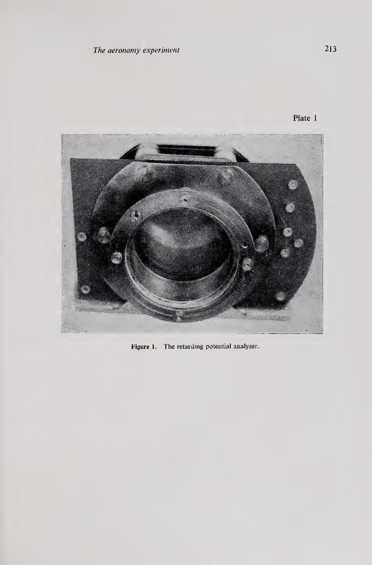
The aeronomy experiment 213
Plate 1
Figure 1. The retarding potential analyser.


The x-ray astronomy experiment
U R RAO,* K KASTURIRANGAN, Y K JAIN, ARUN BATRA, V JAYARAMAN, R A GANAGE, D P SHARMA and M S RADHA ISRO Satellite Centre, Peenya, Bangalore 560 058 *Also at the Physical Research Laboratory, Ahmedabad 380 009
MS received 28 April 1977; revised 8 May 1978
Abstract. One of the scientific experiments onboard Aryabhata was designed to detect and measure celestial x-rays in the energy range 2-5 - 155-0 keV. The payload systems comprising proportional counter and scintillation counter ttelescopes were intended for observations in the pointed and scan modes respectively for investigating the emission properties of celestial x-ray sources. The paper presents the details of these telescopes, their inflight performance as well as the nature of the data obtained during the first few orbits.
Keywords. X-rays; proportional counter; scintillation telescope; x-ray spectrum.
1. Introduction
Since the first discovery of strong x-ray emitting objects beyond the confines of the solar system by Giacconi et al (1962), several experiments have been conducted by different groups to observe the universe through this new window of the electro¬ magnetic spectrum. The bulk of the data in this field has been gathered through the US x-ray astronomy satellite, Uhuru, in the 2-20 keV energy range. Detailed sky survey using proportional counter relescopes onboard this satellite (launched on 12 December 1970), has enabled the generation of a series of x-ray catalogues, the latest of which lists 168 galactic and extra-galactic objects as x-ray emitters (Giacconi et al 1974). Figure 1 shows the Uhuru sky-based on the latest catalogue. Besides the detailed mapping, these observations have also revealed the spectral nature as well as the peculiar properties of some of the individual sources. The association of x-ray sources with members of binary systems as in the case of Cyg X-l and Her X-l, where the x-ray star itself is hypothesised to be a highly condensed object such as a black hole or a neutron star, is an important aspect of the study of x-ray astro¬ nomy. The associated time variation effects have also been investigated revealing the existence of intensity changes with time scales of seconds, minutes, hours, days and even months (Giacconi et al 1973, Oda et al 1972, Schreier et al 1971, Agarwal et al 1972, Nakagawa et al 1973, Frontera and Fulgini 1975, Rao et al 1976a). Such time variation studies besides throwing light on the extent of the emitting regions also serve to make unambiguous identification of these sources through correlated observations at optical and radio wavelengths.
At higher energies, the data gathered so far are comparatively meagre owing to the more severe secondary background problems as well as the reduced intensity of
215

216 U R Rao et al
x-ray emission from the sources. Some of the stronger sources such as Sco X-l and Cyg X-l have been observed and studied extensively by balloon borne scintilla¬ tion telescopes and more recently by the OSO-7 satellite (Li and Clark 1974, Baity et al 1973). Again, the time variation effects were of prime interest in these investigations besides extending the information on the energy spectrum to higher energies.
More recently, the discovery of transient celestial phenomena at x-ray and gamma ray energies such as flares in x-ray sources (Kasturirangan et al 1974), the fast appear¬ ance and disappearance of new x-ray sources in a nova-like fashion (Matilsky et al
1972, Jerningan 1975, Eyles et al 1975, Rao et al 1969, 1971, Evans et al 1970, Pounds et al 1975, Harris et al 1969) and the cosmic gamma ray burst (Klebesadel et al 1973, Kasturirangan et al 1975) has added a new dimension to the investiga¬ tions in x-ray astronomy.
The above considerations motivated the design of an x-ray astronomy payload that was flown on the first Indian scientific satellite Aryabhata. In this paper, we present a description of the payload, its testing and qualification as well as the preli¬ minary data obtained from the first few orbits. The results of detailed analysis of the data obtained from this experiment are presented elsewhere (Kasturirangan et al
1976, Rao et al 1976).
2. Scientific objectives
The main aims of the x-ray astronomy experiment onboard Aryabhata were: (i) the determination of flux and energy spectra of x-ray sources in the energy
range 2-5 keV to 155 keV; (ii) the exploration of new/transient x-ray sources with a sensitivity of 0T photon
cm-2 s_1 in the 2-5-18-75 keY and 10~2 photons cm-2 s-1 in the 15-5-155 keV range;
(iii) study of the time variation in the intensity of strong x-ray sources with time scales of the order of a minute or more.

The x-ray astronomy experiment 217
3. X-ray telescopes
The energy range of 2-5-19-75 keV was investigated using a gas proportional counter telescope. The proportional counter was filled with a mixture of argon and carbon dioxide in the ratio of 9 : 1 to a pressure of one atmosphere with an entrance window of 50 micron thick beryllium. It had a sensitive depth of 3 cm for the detection of x-rays. Charged particle-induced events were eliminated by provid¬ ing an additional gas depth of 1-5 cm with an independent anode wire and setting the top anode events in anticoincidence with the bottom anode events. In addition, the pulse shape discrimination (PSD) technique was employed for minimising contamination due to non-x-ray events such as those due to gamma rays. The detector was imparted directionality by the use of a set of cylindrical collimators made out of an aluminium block. The physical configuration of the telescope is shown in figure 2.
The x-ray telescope for the higher energy range (15-5 keV to 155 keV) consisted basically of a Nal (Tl) crystal of 3-8 cm diameter and 4 mm thickness placed in a cylindrical plastic scintillator NE102A anticoincidence wall. The cylindrical graded shield of lead, tin and copper used as the internal lining for the plastic scintil¬ lator imparted the directionality to this telescope. The entire assembly was viewed from the bottom by a Dumont K-2227 photomultiplier of 5 cm cathode diameter. The charged particle-induced events were eliminated by the pulse shape discrimina¬ tion technique, which separated the events in plastic having 10 ns rise-time from
aluminium collimator
50-8 /j Be window
gas fill 90% argon + 9-5% CO2 + 0-5% He
depth of main counter =30mm
depth of anti counter = 1 5 mm
Figure 2. Physical configuration of the proportional counter telescope.

218 U R Rao et al
V D< o o co
13 o
XS
G O
o3 O
8 Oh cn
X 03 H
w 2^
.2 O JVC O o <u 00 V £ o'
<D 4) ,
|1&| 3 Otj! oo a > G c« C &
<d “of.
Vh O
c5 a
O u
G CD o •9S £ *3 <L> c •►r o >> o
2 | 3-0
"3.5 Z £
<D
8 03 £ 2 W 03
r^
I *0 (N
•f) CN
d> X .S3 ■*"* X bO G G o .9 < &
CD <L> O *-< Jai C <D G * G «0
O *■ IT) *
a o
<N u->
a> <u> fci o
(N
m in
I in
N G «•! G
a .a a .2 O 73 o *3
oo 2 G *-<
in aj T—H <U O to i-H CO
in
2 13 3
in © 6 73 G c3
O O 73 ~ c3 73 5-i G O
t> a a o o 6 o
4) a -a xi •5 « •- ** ^
o3 73 o *3
§a &.S .3 < 2 S. 3 &
E E
OO <N
a o
G
a X G
G X
X ■*-» 73
£
3 ia
X & n.
I
<4_ O « 2o 3 o
G G
.2 *5 *-«
<L> a
a .2 -*—> u- & G co
t32 z^
o 2 a a O 3
o o CO 2 .9
<L> 4-» G G
o 8 (D
Jr1 O a o 13 -*-* o c/3 O o 13 +-*
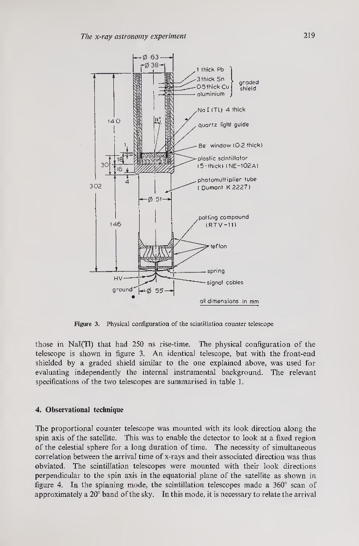
The x-ray astronomy experiment 219
Figure 3. Physical configuration of the scintillation counter telescope
those in NaI(Tl) that had 250 ns rise-time. The physical configuration of the telescope is shown in figure 3. An identical telescope, but with the front-end shielded by a graded shield similar to the one explained above, was used for evaluating independently the internal instrumental background. The relevant specifications of the two telescopes are summarised in table 1.
4. Observational technique
The proportional counter telescope was mounted with its look direction along the spin axis of the satellite. This was to enable the detector to look at a fixed region of the celestial sphere for a long duration of time. The necessity of simultaneous correlation between the arrival time of x-rays and their associated direction was thus obviated. The scintillation telescopes were mounted with their look directions perpendicular to the spin axis in the equatorial plane of the satellite as shown in figure 4. In the spinning mode, the scintillation telescopes made a 360° scan of approximately a 20° band of the sky. In this mode, it is necessary to relate the arrival
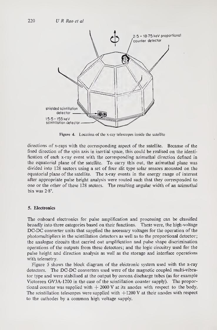
220 U R Rao et al
directions of x-rays with the corresponding aspect of the satellite. Because of the fixed direction of the spin axis in inertial space, this could be realised on the identi¬ fication of each x-ray event with the corresponding azimuthal direction defined in the equatorial plane of the satellite. To carry this out, the azimuthal plane was divided into 128 sectors using a set of four slit type solar sensors mounted on the equatorial plane of the satellite. The x-ray events in the energy range of interest after appropriate pulse height analysis were routed such that they corresponded to one or the other of these 128 sectors. The resulting angular width of an azimuthal bin was 2-8°.
5. Electronics
The onboard electronics for pulse amplification and processing can be classified broadly into three categories based on their functions. These were, the high-voltage DC-DC converter units that supplied the necessary voltages for the operation of the photomultipliers in the scintillation detectors as well as to the proportional detector; the analogue circuits that carried out amplification and pulse shape discrimination operations of the outputs from these detectors; and the logic circuitry used for the pulse height and direction analysis as well as the storage and interface operations with telemetry.
Figure 5 shows the block diagram of the electronic system used with the x-ray detectors. The DC-DC converters used were of the magnetic coupled multi-vibra¬ tor type and were stabilised at the output by corona discharge tubes (as for example Victoreen GV3A-1200 in the case of the scintillation counter supply). The propor¬ tional counter was supplied with -f- 2000 V at its anodes with respect to the body. The scintillation telescopes were supplied with -f-1200 V at their anodes with respect to the cathodes by a common high voltage supply.

The x-ray astronomy experiment 221
DC/DC converter 2000V
shielded scintillotor
detector
DC/DC converter 1200 V
scintillator detector 15-5-155 keV with plastic scintillator
four channel pulse height onalyser
charged particle
four 8 - bit
counters
_ parallel transfer
pulse shape discriminator
charged
pulse shape discriminator
16-bit particleCOunter
16-bit parallel
transfer
four channel pulse height
analyser
-k a
-r 2
simulator
two hundred & fifty six 3-bit counters
12 64 TT
768-bit parallel transfe r
reset/ 1 8 24 sec..
sector decoder |
LSB £ o O L C 0) v) in
MSB f- V)
35 34
840-bit memory
thirty five 24-bit
parallel/ serial convert¬
ers
P S
\ JO
o
3! CO a (\J
* o o c <D
_ Q> 6 0) 0)
D a D O
. o u
. o a m ro
control unit
u a> ^
I in 256 bits/sec | -S
4> O
ground checkout
1-64/65-128 sector selector
code gen. 24 bit
code
nr reset every 8sec
four 7-bit counters
proportionally counter
2-5-15 keV
4 Chi. pulse *fp height 4f analy- ser
IK.
VaVaUer ^ transfer
four 7-bit counter;
'JI'&CJ. poroiiel transfer
U
8i i © >s \ a> H > cO <D
— £ 0) to
o O
o a <D
CO
1 pulse/sec <» £
pulse/32sec £ 9 .8
P' s'
56-bit memory
Y pulse shape
shaper | discriminator
amplifier
charge amplifier
(t> linear amplifier
(^- buffer
% £ 3! 4>
•s <u Bo 3 c 5* o L. o a
Figure 5. Block diagram of the onboard electronics system used for the experiment
As for the analogue electronics, in the case of proportional counter telescope, the output pulses from the first anode were fed to a charge integrating amplifier for impedance transformation and nominal amplification. The pulses were further amplified with a linear amplifier for subsequent pulse height discrimination. The pulses corresponding to the energy interval 2-5-18-75 keV were sorted into 4 energy bins using five comparators which gave a6jas pulse if the input exceeded the threshold. The output of the lowest level discriminator was used to strobe the output from other discriminators to eliminate the occurrence of any spurious output due to the finite rise time of the input pulse resulting in the earlier triggering of a low level discrimi¬ nator compared to an upper one. The charged particle induced effects were reduced by generating a logic pulse corresponding to the output of the second anode after
Proc. (Q—7

222 U R Rao et al
necessary amplification and using it for inhibiting the strobe pulse. Similarly, non¬ x-ray events were separated by pulse shape discrimination of the amplified pulses from the first anode and using them for inhibiting the strobe pulse. To realise this effectively, sufficient delay was provided before strobing, by building into the lowest level discriminator drive a 1 jus delay circuit which, in turn, drove the 4 jus strobe generator. The outputs of the four channels so obtained were stored in 7-bit counters for subsequent processing by telemetry.
In the case of the unshielded telescope, the anode output pulses corresponding to energy losses in the 15-5-155 keV range in Nal(Tl) were analysed into 4 energy channels after suitable amplification by a charge integrating amplifier and appro¬ priate strobing. The charged particle induced events were eliminated by pulse shape discrimination of the pulses tapped from the last dynode by which the pulses corresponding to the plastic anticoincidence shield were identified. The threshold for the plastic anticoincidence was set at a level compatible with the lowest detection threshold for the Nal(Tl) crystal. The output of the four channels were routed through suitable gates to 64 3-bit counters each of which corresponded to a particular sector. The 64 sector information for one half of the 360° azimuthal band of the 7-bit output was obtained by decoding the 6-bit output from solar sensors (excluding the most significant bit (MSB)). The MSB was used for the immediate identifica¬ tion between the two halves of the 180° band of sky that the telescope was looking at for each observation cycle of 24 s as will be described later. The anticoincidence events from the pulse shape discrimination circuit were separately monitored by storing them in a 16-bit memory system. The shielded telescope electronics also used the same logic except that no sector information was derived. Therefore, each of the four channel outputs was separately stored in 8-bit counters.
Onboard data handling was accomplished as follows: the rates corresponding to the proportional counter and the unshielded scintillation counter telescopes, each of four channels and equivalent to a total of 56 bits of information (eight 7-bit counters), were transferred into a parallel-to-serial shift register at 8 s intervals and read out in 8 s by telemetry. Five main frame words per second were allotted to handle the information from the scintillation telescopes. This information stored in the counters was shifted once in 24 s to the parallel-to-serial shift registers which served as buffer memory for the duration of the read out. These telescopes between them represented 816 bits of information, corresponding to 768 bits of the directional and pulse height data of unshielded telescopes, 16 bits of the plastic anticoincidence shield events and 32 bits corresponding to the four channel pulse height counts of the shielded telescope.
The telemetry system read out all the above information in a 24 s cycle at 35 bits/s which, for the allotted 5 words, amounted to 840 bits. The 24 remaining bits were used for the identification of the experiment cycle. The resulting counting capabilities obtained were 35 counts per second per channel for the 15-5-155 keV x-ray events of the unshielded telescope; 10-6 counts per second per channel for the background from the shielded telescope and 2500 counts/second for the plastic antishield events.
6. Detector calibration, test and evaluation
The calibration of the detector systems involved the accurate determination of the
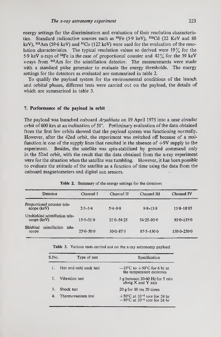
The x-ray astronomy experiment 223
energy settings for the discriminators and evaluation of their resolution characteris¬ tics. Standard radioactive sources such as 55Fe (5-9 keV), 109Cd (22 KeV and 88 keV),241 Am (59-6 keV) and 57Co (122 keV) were used for the evaluation of the reso¬ lution characteristics. The typical resolution values so derived were 19% for the 5-9 keV x-rays of 55Fe in the case of proportional counter and 42% for the 59 keV x-rays from 241Am for the scintillation detector. The measurements were made with a standard pulse generator to evaluate the energy thresholds. The energy settings for the detectors as evaluated are summarised in table 2.
To qualify the payload system for the environmental conditions of the launch and orbital phases, different tests were carried out on the payload, the details of which are summarised in table 3.
7. Performance of the payload in orbit
The payload was launched onboard Aryabhata on 19 April 1975 into a near circular orbit of 600 km at an inclination of 51°. Preliminary evaluation of the data obtained from the first few orbits showed that the payload system was functioning normally. However, after the 42nd orbit, the experiment was switched off because of a mal¬ function in one of the supply lines that resulted in the absence of +9V supply to the experiment. Besides, the satellite was spin-stabilised by ground command only in the 52nd orbit, with the result that the data obtained from the x-ray experiment were for the situation when the satellite was tumbling. However, it has been possible to evaluate the attitude of the satellite as a function of time using the data from the onboard magnetometers and digital sun sensors.
Table 2. Summary of the energy settings for the detectors
Detector Channel I Channel II Channel III Channel IV
Proportional counter tele¬ scope (keV) 2-5-5-4 5-4-9-8 9-8-13-8 13-8-18-85
Unshielded scintillation tele¬ scope (keV) 15-5-31-0 31-0-54-25 54-25-93-0 93-0-155*0
Shielded scintillation tele¬ scope 25-0-50-0 50-0-87-5 87-5-150-0 150-0-250-0
Table 3. Various tests carried out on the x-ray astronomy payload
S.No. Type of test Specification
1. Hot and cold soak test —10°C to +50°C for 6 hr at the temperature extremes
2. Vibration test 5 g between 30-60 Hz for 5 min along X and Y axis
3. Shock test 20 g for 10 ms 20 times
4. Thermovacuum test + 50°C at 10~6 torr for 24 hr — 10°C at 10~6 torr for 24 hr

loti
tud
e
( d
eg
)
224 U R Rao et al
on boord
tim
e
Fig
ure 6
. T
he
counti
ng ra
te
pro
file
s as
reg
iste
red
by
the
two
tele
scopes
in
Orb
it N
o,
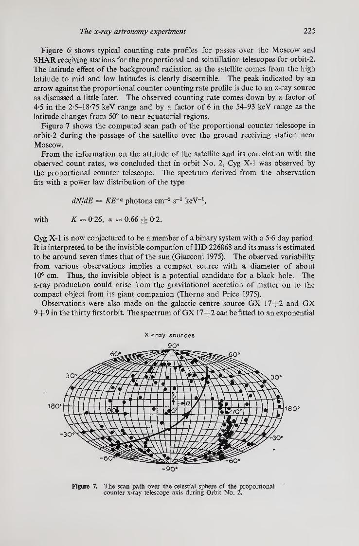
The x-ray astronomy experiment 225
Figure 6 shows typical counting rate profiles for passes over the Moscow and SHAR receiving stations for the proportional and scintillation telescopes for orbit-2. The latitude effect of the background radiation as the satellite comes from the high latitude to mid and low latitudes is clearly discernible. The peak indicated by an arrow against the proportional counter counting rate profile is due to an x-ray source as discussed a little later. The observed counting rate comes down by a factor of 4-5 in the 2-5-18-75 keV range and by a factor of 6 in the 54-93 keV range as the latitude changes from 50° to near equatorial regions.
Figure 7 shows the computed scan path of the proportional counter telescope in orbit-2 during the passage of the satellite over the ground receiving station near Moscow.
From the information on the attitude of the satellite and its correlation with the observed count rates, we concluded that in orbit No. 2, Cyg X-l was observed by the proportional counter telescope. The spectrum derived from the observation fits with a power law distribution of the type
dN/dE = KE~a photons cm-2 s-1 keV-1,
with K — 0*26, a = 0.66 + 0'2.
Cyg X-l is now conjectured to be a member of a binary system with a 5-6 day period. It is interpreted to be the invisible companion of HD 226868 and its mass is estimated to be around seven times that of the sun (Giacconi 1975). The observed variability from various observations implies a compact source with a diameter of about 106 cm. Thus, the invisible object is a potential candidate for a black hole. The x-ray production could arise from the gravitational accretion of matter on to the compact object from its giant companion (Thorne and Price 1975).
Observations were also made on the galactic centre source GX 17+2 and GX 9+9 in the thirty firstorbit. Thespectrum of GX 17+2 can be fitted to an exponential
X -ray sources
90°
-90®
Figure 7. The scan path over the celestial sphere of the proportional counter x-ray telescope axis during Orbit No. 2.

226 U R Rao et al
function in the present case and yields a characteristic value of 9-31 ±0-3 keV. The spectral distribution of GX 9+9 seems to be governed by a power law function with an exponent value of ^1-2 and is suggestive of a non-thermal mechanism for x-ray emission.
The detailed scientific results are published elsewhere (Kasturirangan et al 1976, Rao et al 1976).
8. Conclusion
A payload designed for investigations in x-ray astronomy in the energy range of 2-5 keV to 155 keV was launched onboard the first Indian satellite Aryabhata on 19 April 1975. Based on the limited data available, it is deduced that the payload systems had functioned in orbit according to the expectations thereby validating the various design concepts. The detectors have recorded the fluxes from x-ray sources Cyg X-l, GX 17+2 and GX 9+9 (Kasturirangan et al 1976, Rao et al 1976).
Acknowledgements
We wish to express our sincere thanks to Prof. G E Kocharov, Drs S V Victorov and Naidenov of Leningrad University for valuable advice received during the prepara¬ tion of the payload.
References
Agarwal P C 1972 Study of cosmic x-ray sources using balloon borne detectors. Ph. D. thesis. Uni¬ versity of Bombay
Baity W, Ulmer M, Wheaton W and Peterson L 1973 Nature London Phys. Sci. 245 92 Evans W, Belin R and Conner J 1970 Astrophys J. Lett. 159 L57 Eyles C J, Skinner G K and Willmore A P 1975 Nature London 256 628 Frontera F and Fulgini F 1975 Astrophys. J. 196 597 Giacconi R, Paolini F, Gursky H and Rossi B 1962 Phys. Rev. Lett. 9 439 Giacconi R, Gursky H, Kellogg E, Levinson R, Schreier E and Tananbaum H 1973 Astrophys. J-
184 277 Giacconi R, Murray S, Gursky H, Kellogg E, Schreier E, Matilsky T, Koch D and Tananbaum H
1974 Astrophys. J. Suppl. Series 27 37 Giacconi R 1975 Centre for Astrophysics Preprint No. 304 Harris J, McCracken K G, Francey R and Fenton A 1967 Nature London 215 38 Jerningan G 1975 No. IAU Circular 2817 Aug. 13 Kasturirangan K, Rao U R, Sharma D P, Rastogi R G and Chakravarthy S 1974 Nature London
252 113 Kasturirangan K, Rao U R, Sharma D P, Rastogi RG and Chakravarthy S 1975 Indian J. Radio
Space Phys. 4 203 Kasturirangan K, Rao U R, Sharma D P and Radha M S 1976 Nature London 260 226 Klebesadel R, Strong I, Olson R 1973 Astrophys. J. Lett. 182 L85 Li R and Clark G 1974 Astrophys. J. Lett. 191 L33 Matilsky T, Giacconi R, Gursky H, Kellogg E and Tananbaum H 1972 Astrophys. J. Lett. 174 L53 Nakagawa M, Sakurai H and Kitamura T 1973 13th Int. Cosmic Ray Conf. Denver, USA Paper 671

The x-ray astronomy experiment 227
Oda M, Wada M, Matsuoka M, Miyamoto S, Muranaka N and Ogawar Y 1972 Astrophys. J. Lett.
172 LI 3
Pounds K A, Cooke B A, Ricketts M J, Turner M J, Peacock A and Eadie G 1975 Astrophys. Space
Sci. (to appear) Rao U R, Chitnis E V, Prakasarao A S, Jayanthi U B 1969 Astrophys. J. Lett. 157 LI 27 Rao U R, Chitnis E V, Sharma D P, Prakasarao A S and Jayanthi U B 1971 Nature London 229 248 Rao U R, Kasturirangan K, Sharma D P, Jain A K and Jayanthi U B 1976a Astrophys. Space Sci.
42 193 Rao U R, Kasturirangan K, Sharma D P and Radha M S 1976b Nature London 260 307 Schreier E, Gursky H, Kellogg E, Tananbaum H and Giacconi R 1971 Astrophys. J. Lett. 170 L21 Thorne K S and Price R H 1975 Astrophys. J. Lett. 195 L101

.
-

AUTHOR INDEX
A
Agarwal P C 215 Albus J S 58 Alex T K 57 Allione M S 186 Appa Rao M V K 197 Ashiya R 89
B
Baghdady E J121 Baity W 216 Banerjee A 205 Banks P M 206 Bartley W C 59 Basu S G 119 Batra Arun 215 Belin R 226 Bernier R E 43 Bhamavati A S 163 Bhandari D R 41 Bhaskaranarayana A 89 Bhat R S 175 Bhojaraj H 41 Bland D 56 Bodin W J Jr 133 Bokil A A 151 Brown G H 106 Brown J 80
C
Carver J H 208 Chakravarthy S 226 Chupp E L 197 Chitnis E V 227 Clark G 216 Clemens D B 187, 193 Conner J 226 Collin R E 84 Conover M 56 Cooke B A 227
D
Damle S V 197, 203 Danabalan T L 151 Daniel R R 197, 203 Das U N 89 DaE'athri N R 151 Dunphy P 203 Dash B K 212 Dharma A D 163 Dondi G 187, 188, 193, 194, 196
E
Eadie G 227 El’yasberg P E 176 Engels P D 133 Escobal P R 176 Evans W 216 EylesC J216
F
Faillie V G 133 Fenton A 226 Farley D T 205 Finch H L 43 Fontana A 43 Forrest D J 203 Francey R 226 Franks H J Jr 133 Frontera F 215 Fuke F 133 Fulgini F 215
G
Ganage R A 215 Gaposchkin E M 186 Giacconi R 215, 225, 226, 227 Glazier EVD80 Goel P S 19 Goessl H 133 Golchale G S 197, 203 Gopal Rao V 79 Goswami K K 205 Goswami T K 151 Gruenberg E L 81, 82 Gupta J P 89 Gupta P P 41 Gupta S C 121 Gupta S P 212 Gursky H 226, 227
H
Habib E J 125,133 Hagan F J 196 Hallman R 43 Harris J 216 Harund T 133 Herrick S 176 Higbie P R 203 Hoffman R H 56 Hounam D 133
I
Ingle J V 163
J
Jain A K 227 Jain C L 212 Jain YK 215 Jasik H 106, 113, 114 Jayanthi U B 227 Jayaraman T K 119 Jayaraman V 215 Jenson J 186 Jemingan G 216 John D 79 Joseph George 197, 203

230 Author Index
K
Kahn W D J33 Kaila V K 41 Kalweit C C 67 Kalyanaraman S 79, 119 Kampos B 186 Kanthimathinathan T 29 Kasiviswanathan G A 37 Kasturirangan K 215, 216 227 Katti V R 151 Kellogg E 226, 227 Kitamura T 226 Klebesadel R 216 King-Hele D G 179 Koch D 226 Kork J 186 Kosta S P 105, 116 Kraft D 186 Kraus J D 106 Kreith F 43 Kronmiller G C Jr 133 Kruse K W 121 Kuganento B V 186 Kumar V 205 Kundapurkar R U 197 Kuwand R 121
L
Li R 216 Lakshmeesha V K 105, 116 Lalbowe A G 186 Lavakare P J 197, 203 Levinson R 226
M
Mahadevan V 105, 116 Malik N K 19 Manthiah N 79 Mathe G 198 Matilsky T 216, 226 Matsunaga F M 212 Mathur R S 29 Matsuoka M 227 McCracken K G 68, 226 McCuskey 186 Miller P L 43 Misra R N 205 Mitchel P 208 Miyamoto S 227 Mohanakrishnan G 151 Morrison E 56 Muranaka N 227 Murray S 226 Musick W J 196 Murthy H N 41
N
Nagaraj S R 69 Nalanda V 69 Nair M K 79 Nakagawa M 215 Neilson G 56 Nollet M 133 Narayanan K A 163 Nicholas L 105, 116
O f-i
Oda|MT215 Ogawar Y 227 Olson R 226 Oshima K 43 Oshima Y 43
P
Pal S 105, 106, 108 Pareek P N 205 Pathak P N 187 Patki A V 133 Pattabhiraman K 151 Peacock A 227 Paolini F 226 Peterson L 226 Peterson W D 121 Pounds K A 216 Powers E I 56 Prakasarao A S 227 Prakash S 205, 212 Prasad S N 119 Prasad V 41 Pratap V R 163 Price R H 225
R
Radha M S 215, 226, 227 Rajangam R K 69 Rajasingh C K 175 Raju D V 69 Rajyalaskhmi P S 69 Ramakrishnan S Y 29 Rao K N S 105 Rao V S 105 Rao U R 1, 68, 115, 215, 216, 226 Rastogi R G 226 Reddy P K105, 116 Ricketts M J 227 Robertson R L 176, 179 Rogers E E 23 Rossi B 226
S
Saha M K 79, 106, 119 Sakai H 212 Sakurai H 226 Sambasiva Rao M 119 Sapra O P 163 Sastry M L N 79 Sathyanarayan M N 151 Savalgi N S 29 Scafer M K 186 Schlenk B 198 Schreier E 215, 226 Selvaraj I 151 Semple E C 43 Seshadri B V 89 Seshaiah R 69 Shaffer H W 125 Shamanna K N 105 Shamaprakash B K 163 Sharma D P 215, 226, 227 Shirke J S 205 Singal Y K 89 Singh R S 205 Sinitrsyn V N 186 Sivaswamy R 69

Author Index 231
Skinner G K 226 Sommerville D 56 Sterne T E 179 Srinivasan P N 19 Strong I 226 Subbaraya B H 205, 212 Subbiah S 163 Subramanian M 29 Sudarshan Sarpangal 29 Suri A N 203
T
Tananbaum H 226, 227 Tand J 133 Tarsem Singh 163 Thomas G E 206 Thomas V A 151 Thome K S 225 Timmins A R 56 Townserd G 186 Tsai C 203 Turner M J 227 Tyagi RN 119
U
Ulmer M 226
V
Varadarajulu V P V 57 Venkataramana D 89 Venkataramanan S T 29 Venkateshaiah C N 69 Venkateswaran P R 57 Viterbi A J 127 Vogt R 56
W
Wada M 227 Wales I M 186 Walter H G 186 Watanabe K 210 Wheaton W 226 Wiebelt J A 43 Will more A P 226 Wolf E A 113, 114 Wolverton R W 186 Woodward O M 106

.
.
*

SUBJECT INDEX
Analog-digital converter The telemetry system 69
Hydrogen geocorona The aeronomy experiment 205
Antennas Antenna systems for the Aryabhata mission 105
Interferometry system The tracking system 119
Array voltage limiter The power system 29
Ionosphere-magnetosphere coupling The aeronomy experiment 205
Aryabhata
An overview of the Aryabhata project 1 Link estimate
The communication system 79
Attitude control The stabilisation system 19
Magnetometer Attitude and temperature sensors 57
Attitude sensors Attitude and temperature sensors 57
Mechanical integration System integration 151
Bit error probability The communication system 79
Noise figure The communication system 79
Cable system The ground checkout system 163
Orbit Orbit computations 175
Changeover system The telemetry system 69
Power conditioning and control The power system 29
Coding The telecommand system 89
Power generation The power system 29
Command systems The telecommand system 89
Premodulation filter The telemetry system 69
Computation Orbit computations 175
Proportional counter The x-ray astronomy experiment 215
Cost of spacecraft A statistical analysis of weight and cost para¬
Protective devices The power system 29
meters of spacecraft with special reference to Pulse code modulation Aryabhata 187 The telemetry system 69
Design
The thermal control system 41
Satellite
Orbit computations 175
Doppler system Antenna systems for the Aryabhata mission 105
The tracking system 119 Satellite design
Electrical integration An overview of the Aryabhata project 1
System integration 151 Satellite instrumentation
Electromagnetics An experiment to detect energetic neutrons and
Antenna systems for the Aryabhata mission 105 gamma rays from the sun 197
F region anomaly The aeronomy experiment 205
Satellite integration philosophy
System integration 151
Flight performance The thermal control system 41
Satellite performance An overview of the Aryabhata project 1
Ground checkout system The ground checkout system 163
Satellite qualification An overview of the Aryabhata project 1
Grounding The power system 29
Satellite stabilisation The stabilisation system 19
Hybrid coupler satellite communication The communication system 79
Satellite structure The structure 135

234 Subject Index
Satellite technology An overview of the Aryabhata project
Satellite telecommand The telecommand system
Satellite telemetry The telemetry system
Satellite thermal control The thermal control system
Satellite tracking system The tracking system
Scintillation telescope The x-ray astronomy experiment
Side band power The communication system
Solar array The power system
Solar neutron experiment An experiment to detect energetic neutrons gamma rays from the sun
Spin angle clock Attitude and temperature sensors
Spin-stabilisation The stabilisation system
Spin-up system The stabilisation system
Spinning satellite
Attitude^and^temperature sensors 57
Storage
The power system 29
Structural configuration The structure 135
Structural design The structure 135
Sub-carrier oscillator The telemetry system 69
System layout System integration 151
Testing philosophy System integration 151
Tone-ranging system The tracking system 119
Weight of spacecraft A statistical analysis of weight and cost para¬ meters of spacecraft with special reference to Aryabhata 187
X-rays The x-ray astronomy experiment 215
X-ray spectrum The x-ray astronomy experiment 215
1
89
69
41
119
215
79
29
and 197
57
19
19


Related Documents


![References - Home - Springer978-1-4612-0803-7/1.pdf · 312 References [11] Aryabhata Aryabhatiya of Aryabhata, New Delhi: ... Trans. Charles Pinter and Helen Kline, New York: Dover,](https://static.cupdf.com/doc/110x72/5b82af807f8b9a315b8b8d18/references-home-springer-978-1-4612-0803-71pdf-312-references-11-aryabhata.jpg)


