The Arsenal of Democracy: Production and Politics During WWII

The Arsenal of Democracy:Production and Politics During WWII

Paul Rhode∗ James M. Snyder, Jr.† Koleman Strumpf‡

December 5, 2016

Abstract

We study the geographic distribution of military supply contracts during WorldWar II. This is a unique case, since over $3 trillion current day dollars was spent,and there were concerns that the country’s future hinged on the war outcome. Wefind robust evidence consistent with the hypothesis that economic factors dominatedthe allocation of supply contracts, and that political factors—or at least winning the1944 presidential election—were at best of secondary importance. General industrialcapacity in 1939, as well as specialized industrial capacity for aircraft production, arestrong predictors of contract spending across states. On the other hand, electoralcollege pivot probabilities are at best weak predictors of contract spending, and underthe most plausible assumptions they are essentially unrelated to spending. This istrue not only for total spending over the entire period 1940-1944, but also for shorterperiods leading up to the election in November 1944. That is, we find no evidence ofan electoral cycle in the distribution of funds.

Keywords: Distributive politics, government spending, presidential elections

JEL Classification:

∗Department of Economics, University of Michigan†Department of Government, Harvard University, and NBER‡School of Business, University of Kansas

1

1 Introduction

During the Second World War, the federal government assumed an unprecedented degree of

control over the U.S. economy. At the peak, the share of federal government expenditures

in GNP soared to 44 percent, a level never attained before or since. (The level has not even

exceeded 25 percent in the post-WWII era.) In addition to enrolling 16.4 million Americans—

about one-eighth of the 1940 population—in the armed forces, the federal government spent

$196 billion between 6/1940 and June 1945 on military supply contracts and $31 billion

on investments in new production facilities. In 2014 dollars, this is equivalent to roughly

$3.1 trillion. Surprisingly, although this war effort probably represented the largest single

economic intervention by the federal government in U.S. history, the political economy of

these spending flows has been subject to relatively little systematic, scholarly investigation.

This paper uses state-level economic and political data to investigate the relative impor-

tance of political and economic (strategic) factors in accounting for the geographic allocation

of World War II -era military spending, both for major war supply contracts and for new

facility projects. More specifically, we study the allocation of supply contracts and new

facilities across all U.S. states during the period September 1940 through 10/1944.

Following an extensive empirical and theoretical literature on distributive politics in the

U.S., we focus on one of the incumbent party’s main goals—winning the next presidential

election.1 To measure the electoral importance of each state we employ a model similar to

that in Stromberg (2008). Simulations based on this model yield estimates of the relative

probability that each state would be pivotal in the electoral college in the 1944 presidential

election. The model incorporates four key elements: (i) How close the average two-party

vote in each state is to 50%; (ii) How variable the two-party vote is in each state; (iii) How

many electoral votes the state has per-capita; and (iv) How correlated the two-party vote

shares are across states.

To measure the economic/strategic importance of each state we use estimates of industrial

capacity at the beginning of the war. States such as Connecticut, Michigan, New Jersey and

Pennsylvania already had large factories producing automobiles, trucks, airplanes, ships,

steel, and so on. These states also had a large stock of human capital ready to do work—

many thousands of workers with many years of experience in factory work. Converting this

1See, e.g., Wright (1974), Wallis (1987, 1998, 2001), Brams and Davis (1974, 1982), Colantoni, Levesqueand Ordeshook (1975), Nagler and Leighley (1992), Shaw (2006), Shor (2006), Stromberg (2008), Hudak(2014).

2

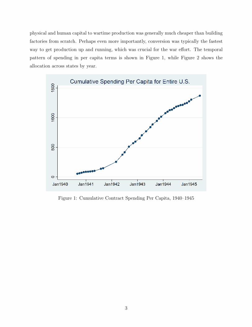
physical and human capital to wartime production was generally much cheaper than building

factories from scratch. Perhaps even more importantly, conversion was typically the fastest

way to get production up and running, which was crucial for the war effort. The temporal

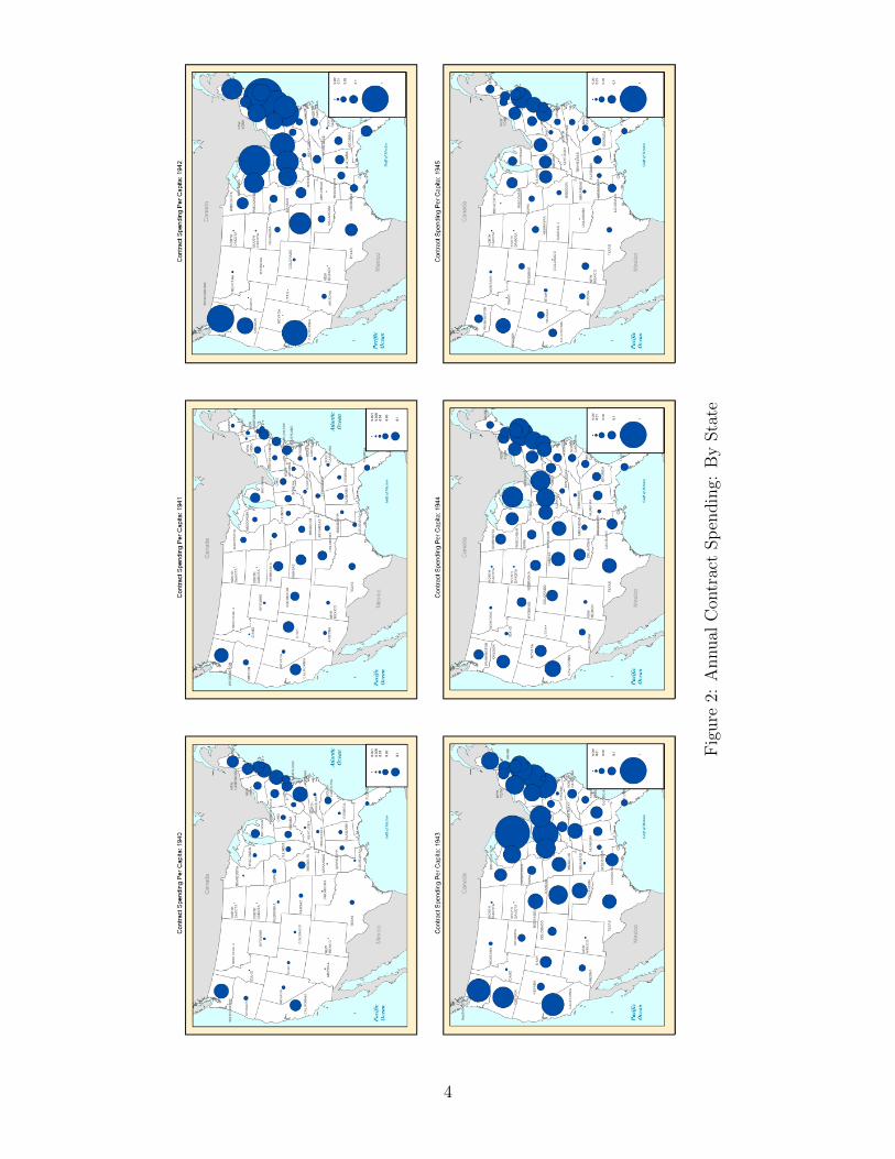
pattern of spending in per capita terms is shown in Figure 1, while Figure 2 shows the

allocation across states by year.

Figure 1: Cumulative Contract Spending Per Capita, 1940–1945

3

Fig

ure

2:A

nnual

Con

trac

tSp

endin

g:B

ySta

te

4

Our findings are easily summarized. We find robust evidence consistent with the hy-

pothesis that economic factors strongly influenced the allocation of supply contracts, and

that political factors—or at least winning the 1944 presidential election—were at best of

secondary importance. General industrial capacity in 1939, as well as specialized industrial

capacity for aircraft production, are strong predictors of contract spending across states.

On the other hand, electoral college pivot probabilities are at best weak predictors of con-

tract spending, and under the most plausible assumptions they are essentially unrelated to

spending (as discussed below, a key free parameter is how responsive votes are to spending,

and we use values based on estimates which which relate voting preferences in Gallup polls

to both World War II and New Deal spending). This is true not only for total spending

over the entire period 1940-1944, but also for shorter periods leading up to the election in

November 1944. Thus, in addition to finding no overall effect of pivot probabilities, we also

find no evidence of an electoral cycle in the distribution of funds.

It is possible, of course, that pragmatic concerns related to winning the war dominated

narrow distributional concerns because the enormous stakes involved. As Churchill famously

argued as the Battle of Britain began, “Upon this battle depends the survival of Christian

civilization... If we fail, then the whole world, including the United States, including all that

we have known and cared for, will sink into the abyss of a new Dark Age.” It might not be

surprising, therefore, to find the U.S. government acting as if it placed an extremely high

value on social welfare—the “public good” of defeating Germany and Japan.

It is also possible that pragmatic concerns related to winning the war dominated narrow

distributional concerns for electoral reasons. A number of political economy models incor-

porate both public goods and distributive goods.2 One (unsurprising) result in these papers

is that elected officials will provide public goods rather than distributive goods if the public

goods are valued enough by voters relative to the distributive goods. In these circumstances,

it is difficult to distinguish a concern for social welfare from a concern for votes.3

We find evidence consistent with this hypothesis in survey data. For example, as the

war proceeded and it became clearer that the allies were winning—especially after D-Day in

June 1944—respondents became more confident that the war was more likely to end quickly

if the Democrats remained in power than if the Republicans held power.

2See, e.g., Leblanc, Snyder and Tripathi (2000), Lizzeri and Persico (2005), Battaglini and Coate (2008),Volden and Wiseman (2007), and Cardona and Rubı-Barcelo (2013).

3See also Becker (1983), which predicts that under “pluralism,” in which a large number of interest groupscompete for influence, we should also expect relatively outcomes.

5

At a minimum, our evidence suggests that model that focus exclusively on “tactical

distributional politics”—e.g., Lindbeck and Weibull (1987), Dixit and Londregan (1995,

1996), McCarty (2000), Stromberg (2008), Primo and Snyder (2008)—might be useful in

predicting government behavior in times of national crisis.

2 Background

During the Second World War, the federal government assumed an unprecedented degree

of control over the US economy. The federal government spent $196 billion between 6/1940

and June 1945 on military supply contracts and $31 billion on investments in new facilities.

Relative to the 1940 total population, per capita spending over this five-year period averaged

$1,813 in current dollars or almost $24,800 in 2014 purchasing power. In real annual per

capita terms, domestic procurement spending during World War II was about than four-and-

one-half times higher than the New Deal era spending which has attracted so much scholarly

attention.

In the interwar period, the US government spent only 1-2 percent of GDP on the military.

Most money for supplies and arms was allocated according to rigidly specified competitive

procedures. Procurement officers would advertise for clearly defined quantities and qualities

for a specific item, invited bids, and award the contract to the lowest qualified bidder. The

federal government also imposed profit limits on aircraft and shipbuilding contracts under

the 1934 Vinson-Trammel and 1936 Merchant Marine Acts.

The outbreak of full-scale war in September 1939 led to dramatic changes in “business as

usual.” Table 1 offers a condensed timeline of the evolution of government agencies in charge

of procurement and industrial mobilization over the 1939-45 period. The expediting acts of

June 28 and July 2, 1940, allowed negotiated, cost-plus-a-fixed-fee contracts and payment

before delivery. While procurement authorities continued to use competitive bidding for

small contracts, the vast majority of procurement contracts shifted to a negotiated basis. In

October 1940, the federal government also eliminated profit ceilings on defense contracts,

using excess-profit taxes in their place. A series of civilian-run bureaucracies were created

to facilitate the war production effort.

In May 1940, Roosevelt used his war powers to establish Advisory Commission of the

Council for National Defense (NDAC). The NDAC begat the Office of Production Man-

agement (OPM) which begat the War Production Board (WPB) which begat the Civilian

6

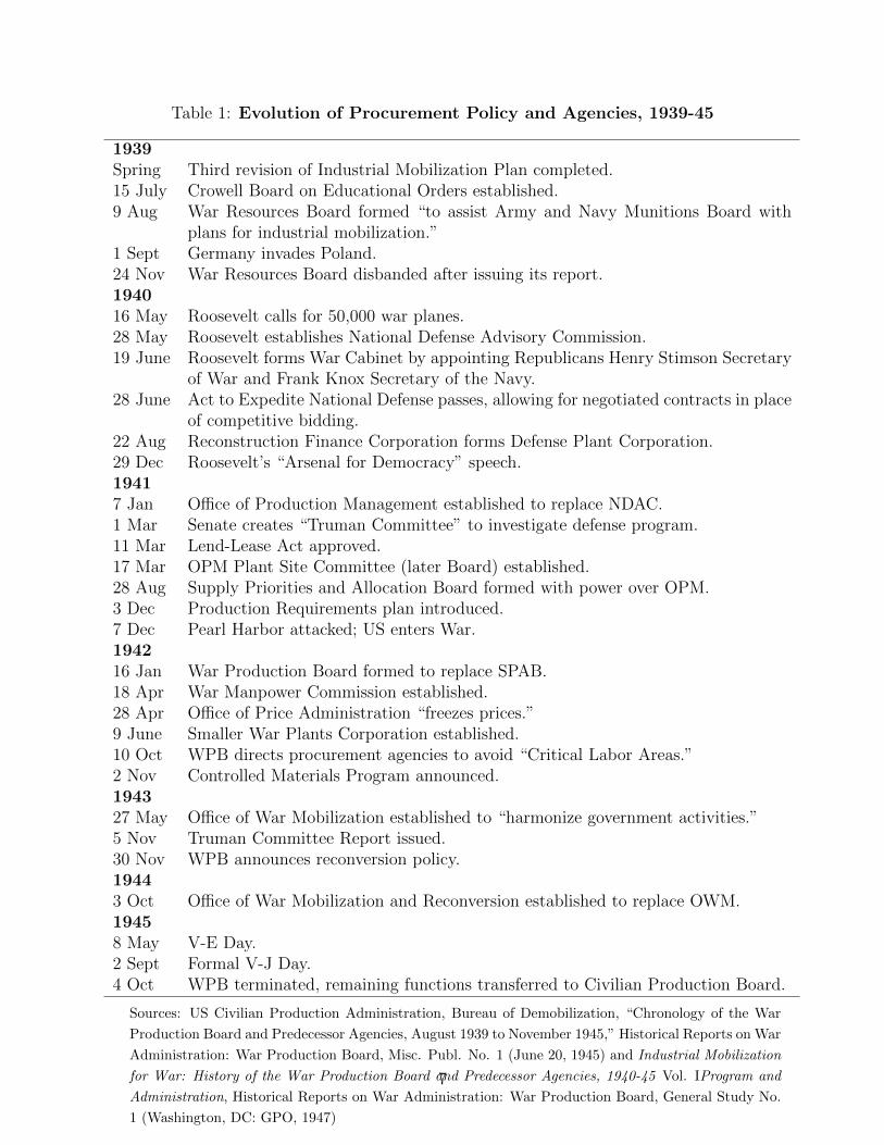
Table 1: Evolution of Procurement Policy and Agencies, 1939-45

1939Spring Third revision of Industrial Mobilization Plan completed.15 July Crowell Board on Educational Orders established.9 Aug War Resources Board formed “to assist Army and Navy Munitions Board with

plans for industrial mobilization.”1 Sept Germany invades Poland.24 Nov War Resources Board disbanded after issuing its report.194016 May Roosevelt calls for 50,000 war planes.28 May Roosevelt establishes National Defense Advisory Commission.19 June Roosevelt forms War Cabinet by appointing Republicans Henry Stimson Secretary

of War and Frank Knox Secretary of the Navy.28 June Act to Expedite National Defense passes, allowing for negotiated contracts in place

of competitive bidding.22 Aug Reconstruction Finance Corporation forms Defense Plant Corporation.29 Dec Roosevelt’s “Arsenal for Democracy” speech.19417 Jan Office of Production Management established to replace NDAC.1 Mar Senate creates “Truman Committee” to investigate defense program.11 Mar Lend-Lease Act approved.17 Mar OPM Plant Site Committee (later Board) established.28 Aug Supply Priorities and Allocation Board formed with power over OPM.3 Dec Production Requirements plan introduced.7 Dec Pearl Harbor attacked; US enters War.194216 Jan War Production Board formed to replace SPAB.18 Apr War Manpower Commission established.28 Apr Office of Price Administration “freezes prices.”9 June Smaller War Plants Corporation established.10 Oct WPB directs procurement agencies to avoid “Critical Labor Areas.”2 Nov Controlled Materials Program announced.194327 May Office of War Mobilization established to “harmonize government activities.”5 Nov Truman Committee Report issued.30 Nov WPB announces reconversion policy.19443 Oct Office of War Mobilization and Reconversion established to replace OWM.19458 May V-E Day.2 Sept Formal V-J Day.4 Oct WPB terminated, remaining functions transferred to Civilian Production Board.

Sources: US Civilian Production Administration, Bureau of Demobilization, “Chronology of the War

Production Board and Predecessor Agencies, August 1939 to November 1945,” Historical Reports on War

Administration: War Production Board, Misc. Publ. No. 1 (June 20, 1945) and Industrial Mobilization

for War: History of the War Production Board and Predecessor Agencies, 1940-45 Vol. IProgram and

Administration, Historical Reports on War Administration: War Production Board, General Study No.

1 (Washington, DC: GPO, 1947)

7

Production Administration (CPA). An additional layer of bureaucracy, first the Supply Pri-

orities and Allocations Board (SPAB) and later the Office of War Mobilization (OWM), was

imposed on top of these agencies. Although the agency names changed, the leading actors

did not. These included William S. Knudson, a dollar-a-year man on leave from General

Motors, Donald M. Nelson, another dollar-a-year man who had been an executive at Sears-

Roebuck, and Sidney Hillman, a former union chief. Other principals were Henry Stimson

and Frank Knox, two Republicans that Roosevelt had appointed Secretaries of War and

Navy, respectively, in the summer of 1940.

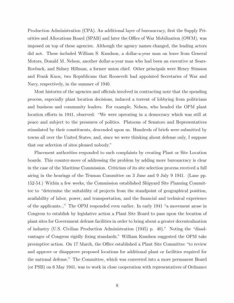
Most histories of the agencies and officials involved in contracting note that the spending

process, especially plant location decisions, induced a torrent of lobbying from politicians

and business and community leaders. For example, Nelson, who headed the OPM plant

location efforts in 1941, observed: “We were operating in a democracy which was still at

peace and subject to the pressures of politics. Platoons of Senators and Representatives

stimulated by their constituents, descended upon us. Hundreds of briefs were submitted by

towns all over the United States, and, since we were thinking about defense only, I suppose

that our selection of sites pleased nobody.”

Placement authorities responded to such complaints by creating Plant or Site Location

boards. This counter-move of addressing the problem by adding more bureaucracy is clear

in the case of the Maritime Commission. Criticism of its site selection process received a full

airing in the hearings of the Truman Committee on 3 June and 9 July 9 1941. (Lane pp.

152-54.) Within a few weeks, the Commission established Shipyard Site Planning Commit-

tee to “determine the suitability of projects from the standpoint of geographical position,

availability of labor, power, and transportation, and the financial and technical experience

of the applicants...” The OPM responded even earlier. In early 1941 “a movement arose in

Congress to establish by legislative action a Plant Site Board to pass upon the location of

plant sites for Government defense facilities in order to bring about a greater decentralization

of industry (U.S. Civilian Production Administration (1945) p. 40).” Noting the “disad-

vantages of Congress rigidly fixing standards,” William Knudsen suggested the OPM take

preemptive action. On 17 March, the Office established a Plant Site Committee “to review

and approve or disapprove proposed locations for additional plant or facilities required for

the national defense.” The Committee, which was converted into a more permanent Board

(or PSB) on 6 May 1941, was to work in close cooperation with representatives of Ordnance

8

Department, the Army Air Corps, and the Navy Department (pp. 40-42).

“Such factors as availability of labor, transportation facilities, housing, waterpower, com-

munity services and attitude, sources of raw materials and destination of the finished prod-

ucts, and the general relation of the new plants to the over-all distribution of manufacturing

facilities in the country were carefully examined. The board was anxious to avoid, if possible,

the building of plants in already highly industrialized and congested areas” (p. 56). “The

Plant Site Board did endeavor to locate new facilities away from highly industrialized areas.

In part the location of new facilities was determined by strategic reasons... According to

Nelson, supply contracts followed the location of industry; but new facilities were planned

to follow at least partial decentralization” (p. 58).

PSB policy called for preserving “the area north of the Mason-Dixon line and east of the

Mississippi River for defense manufacturing requiring highly skilled labor, such as aircraft

engines, and indicating that approval for other types of facilities in this area would, in general,

be given only in exceptional circumstances.” The Board (pp. 60-61) “was aware on the

undesirability of further concentrating aircraft facilities in southern California, of expanding

plant facilities in the Detroit area, of enlarging shipbuilding plants around Camden, New

Jersey, and of locating more plants at Bendix, Philadelphia, Rochester, and other highly

industrialized centers.” It acted primarily as a “negative planning unit” which frequently

initially vetoed proposed sites and urged the procurement officials look in less congested

areas. “In view of the urgency for speeding up production, however, the Plant Site Board

was reluctant to exercise this (veto) power for fear of impeding the defense effort” (pp.

59-61). The PSB and other civilian authorities generally allowed the military procurement

officers to contract where they pleased, and in turn, the procurement authorities allowed

their manufacturing suppliers to produce and invest where they saw fit.

Politics or peacetime objectives played crucial roles in some decisions. In 1938, the US

Maritime Commission received congressional permission to grant contracts to shipyards in

the South and West despite their higher cost structures (Lane, pp. 102-04). Although

the performance of southern shipbuilders remained below eastern levels in the early 1940s,

the Commission followed the administrations wishes by granting some wartime contracts

to southern yards. Costs and productivity on the West Coast did reach parity with the

east by the early 1940s, leading to the placement of large share of contracts there during

the war. But the pre-war West possessed no modern integrated steel plants and hence no

9

capacity to produce ship plates locally. In response, Roosevelt had the federal government

help finance two new steel plants (at Geneva UT and Fontana, CA). In addition, there were

numerous accusations of influence peddling, kickbacks, and conflicts of interest regarding

defense spending. Notable contracting scandals involved Thomas Corcoran, a New Deal

political operative, General Bennett Meyers of the Army Air Crop, Representative Andrew

May of Kentucky, chair of the House Committee on Military Affairs, and Senator Theodore

Bilbo of Mississippi.

3 Data and Summary Statistics

The state-level monthly (approx.) military spending variables– contract and facilities spending–

are from various economic reports published by the National Industrial Conference Board,

hearings of the U.S. House Select Committee Investigating National Defense Migration, and

the U.S. War Production Board, Statistics of War Production. See the data appendix for

details.

The manufacturing employment variables, including the number of wage-earners in total,

in aircraft (SIC 372) and shipbuilding (SIC 373) in 1939 are from US Bureau of the Census,

Census of Manufactures: 1947, Vo. 3, Area Statistics (Washington, DC: GPO, 1950).

The state-level data on elections for U.S. president, U.S. senator, and state governor are

from ICPSR study number 2 (Candidate Name and Constituency Totals, 1788-1990).

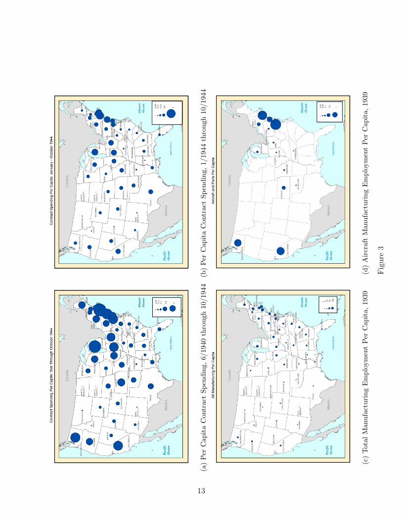
Figures 3a and 3b show the distribution of two of the dependent variables we study—

contract spending per-capita for the entire war up to November 1944 (i.e. 6/1940 through

10/1944), and contract spending per-capita from January to November of 1944 only. The

maps show that many states in the northeast and industrial midwest—Connecticut, Rhode

Island, Delaware, New Jersey, Michigan, Indiana and Ohio—received much more in contract

spending per capita than the average state. The three states bordering the Pacific also

fared quite well in terms of contracts. However, the map also shows that some states less

associated with the industrial heartland—e.g., Kansas, Missouri, Nebraska, Oklahoma, and

Texas, also received more in contract spending that the average state.

Figures 3c and 3d show the distribution of the other key independent variables—total

manufacturing employment per-capita and aircraft manufacturing employment per-capita—

across the U.S. states. Three features stand out. First, overall manufacturing employment

was distributed relatively uniformly compared to the other variables (hence no large dots).

10

Second, it is nonetheless clear that total manufacturing employment per-capita was a bit

larger in northeast and industrial midwest than in other regions. There are a few exceptions,

such as North and South Carolina, Georgia, and Virginia, which had substantial numbers

of manufacturing employees. Third, aircraft manufacturing employment was highly concen-

trated in a few states.

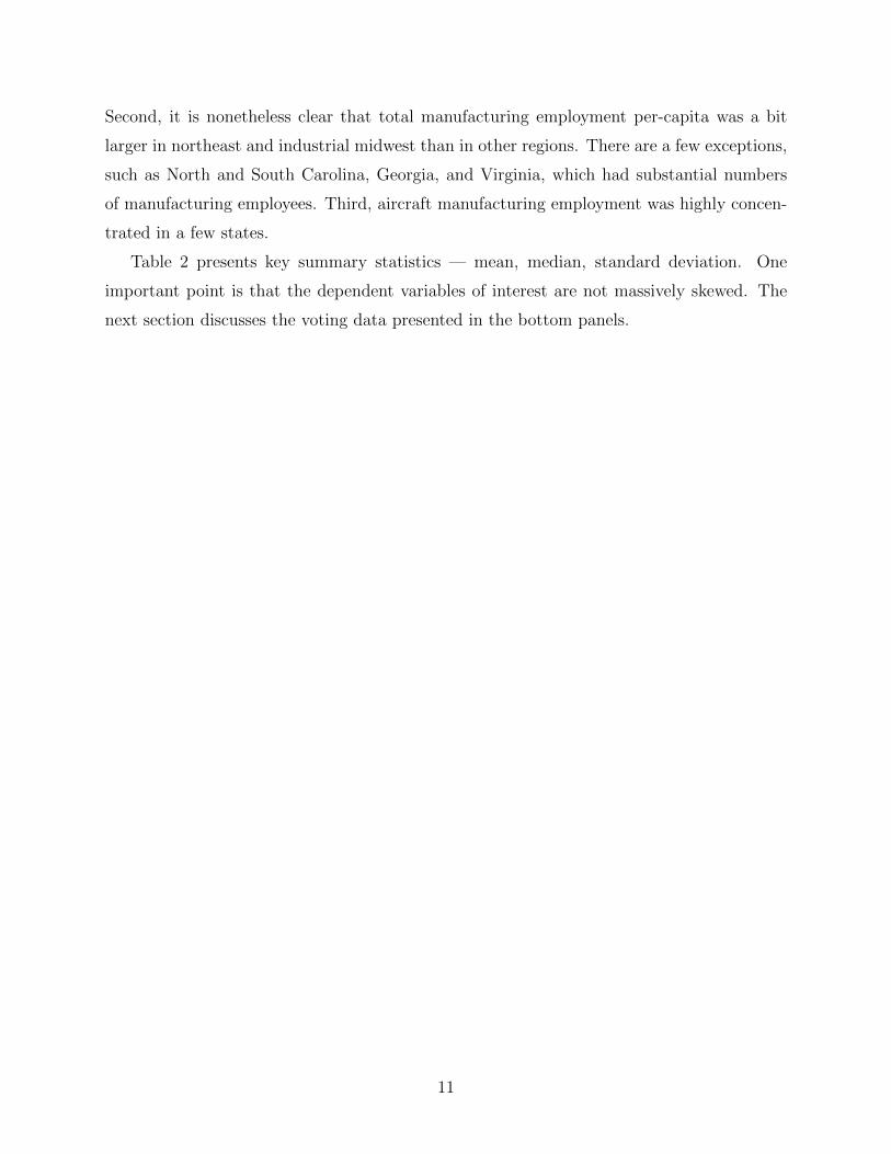
Table 2 presents key summary statistics — mean, median, standard deviation. One

important point is that the dependent variables of interest are not massively skewed. The

next section discusses the voting data presented in the bottom panels.

11

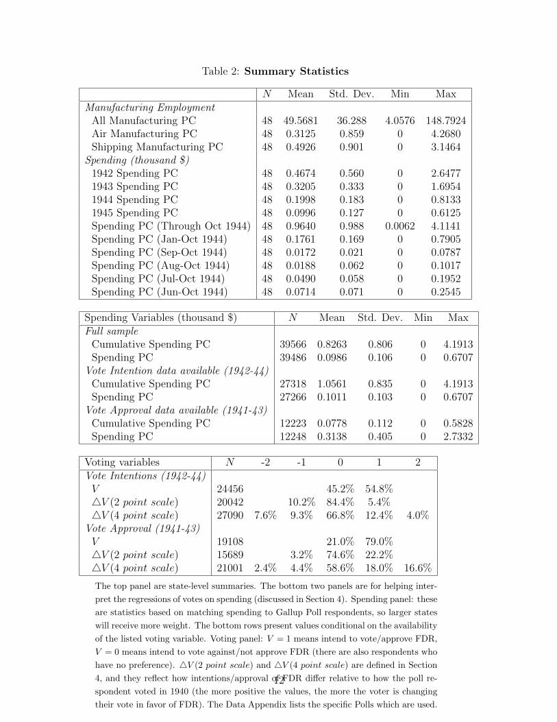
Table 2: Summary Statistics

N Mean Std. Dev. Min MaxManufacturing Employment

All Manufacturing PC 48 49.5681 36.288 4.0576 148.7924Air Manufacturing PC 48 0.3125 0.859 0 4.2680Shipping Manufacturing PC 48 0.4926 0.901 0 3.1464

Spending (thousand $)1942 Spending PC 48 0.4674 0.560 0 2.64771943 Spending PC 48 0.3205 0.333 0 1.69541944 Spending PC 48 0.1998 0.183 0 0.81331945 Spending PC 48 0.0996 0.127 0 0.6125Spending PC (Through Oct 1944) 48 0.9640 0.988 0.0062 4.1141Spending PC (Jan-Oct 1944) 48 0.1761 0.169 0 0.7905Spending PC (Sep-Oct 1944) 48 0.0172 0.021 0 0.0787Spending PC (Aug-Oct 1944) 48 0.0188 0.062 0 0.1017Spending PC (Jul-Oct 1944) 48 0.0490 0.058 0 0.1952Spending PC (Jun-Oct 1944) 48 0.0714 0.071 0 0.2545

Spending Variables (thousand $) N Mean Std. Dev. Min MaxFull sample

Cumulative Spending PC 39566 0.8263 0.806 0 4.1913Spending PC 39486 0.0986 0.106 0 0.6707

Vote Intention data available (1942-44)Cumulative Spending PC 27318 1.0561 0.835 0 4.1913Spending PC 27266 0.1011 0.103 0 0.6707

Vote Approval data available (1941-43)Cumulative Spending PC 12223 0.0778 0.112 0 0.5828Spending PC 12248 0.3138 0.405 0 2.7332

Voting variables N -2 -1 0 1 2Vote Intentions (1942-44)V 24456 45.2% 54.8%4V (2 point scale) 20042 10.2% 84.4% 5.4%4V (4 point scale) 27090 7.6% 9.3% 66.8% 12.4% 4.0%

Vote Approval (1941-43)V 19108 21.0% 79.0%4V (2 point scale) 15689 3.2% 74.6% 22.2%4V (4 point scale) 21001 2.4% 4.4% 58.6% 18.0% 16.6%

The top panel are state-level summaries. The bottom two panels are for helping inter-

pret the regressions of votes on spending (discussed in Section 4). Spending panel: these

are statistics based on matching spending to Gallup Poll respondents, so larger states

will receive more weight. The bottom rows present values conditional on the availability

of the listed voting variable. Voting panel: V = 1 means intend to vote/approve FDR,

V = 0 means intend to vote against/not approve FDR (there are also respondents who

have no preference). 4V (2 point scale) and 4V (4 point scale) are defined in Section

4, and they reflect how intentions/approval of FDR differ relative to how the poll re-

spondent voted in 1940 (the more positive the values, the more the voter is changing

their vote in favor of FDR). The Data Appendix lists the specific Polls which are used.

12

(a)

Per

Cap

ita

Con

trac

tS

pen

din

g,6/

1940

thro

ugh

10/1

944

(b)

Per

Cap

ita

Con

trac

tS

pen

din

g,1/

1944

thro

ugh

10/1944

(c)

Tot

alM

anu

fact

uri

ng

Em

plo

ym

ent

Per

Cap

ita,

1939

(d)

Air

craf

tM

anu

fact

uri

ng

Em

plo

ym

ent

Per

Cap

ita,

1939

Fig

ure

3

13

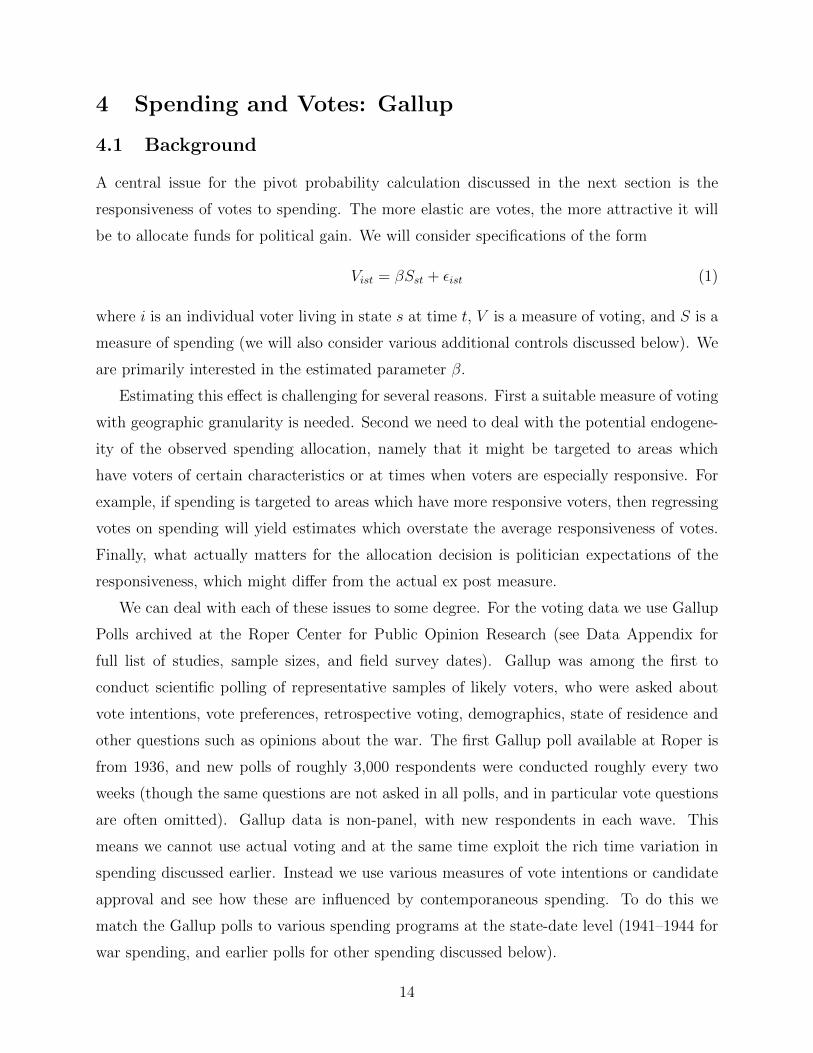
4 Spending and Votes: Gallup

4.1 Background

A central issue for the pivot probability calculation discussed in the next section is the

responsiveness of votes to spending. The more elastic are votes, the more attractive it will

be to allocate funds for political gain. We will consider specifications of the form

Vist = βSst + εist (1)

where i is an individual voter living in state s at time t, V is a measure of voting, and S is a

measure of spending (we will also consider various additional controls discussed below). We

are primarily interested in the estimated parameter β.

Estimating this effect is challenging for several reasons. First a suitable measure of voting

with geographic granularity is needed. Second we need to deal with the potential endogene-

ity of the observed spending allocation, namely that it might be targeted to areas which

have voters of certain characteristics or at times when voters are especially responsive. For

example, if spending is targeted to areas which have more responsive voters, then regressing

votes on spending will yield estimates which overstate the average responsiveness of votes.

Finally, what actually matters for the allocation decision is politician expectations of the

responsiveness, which might differ from the actual ex post measure.

We can deal with each of these issues to some degree. For the voting data we use Gallup

Polls archived at the Roper Center for Public Opinion Research (see Data Appendix for

full list of studies, sample sizes, and field survey dates). Gallup was among the first to

conduct scientific polling of representative samples of likely voters, who were asked about

vote intentions, vote preferences, retrospective voting, demographics, state of residence and

other questions such as opinions about the war. The first Gallup poll available at Roper is

from 1936, and new polls of roughly 3,000 respondents were conducted roughly every two

weeks (though the same questions are not asked in all polls, and in particular vote questions

are often omitted). Gallup data is non-panel, with new respondents in each wave. This

means we cannot use actual voting and at the same time exploit the rich time variation in

spending discussed earlier. Instead we use various measures of vote intentions or candidate

approval and see how these are influenced by contemporaneous spending. To do this we

match the Gallup polls to various spending programs at the state-date level (1941–1944 for

war spending, and earlier polls for other spending discussed below).

14

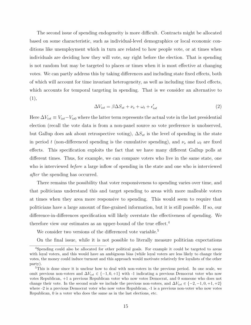
The second issue of spending endogeneity is more difficult. Contracts might be allocated

based on some characteristic, such as individual-level demographics or local economic con-

ditions like unemployment which in turn are related to how people vote, or at times when

individuals are deciding how they will vote, say right before the election. That is spending

is not random but may be targeted to places or times when it is most effective at changing

votes. We can partly address this by taking differences and including state fixed effects, both

of which will account for time invariant heterogeneity, as well as including time fixed effects,

which accounts for temporal targeting in spending. That is we consider an alternative to

(1),

∆Vist = β∆Sst + νs + ωt + ε′ist (2)

Here ∆Vist ≡ Vist−Vis0 where the latter term represents the actual vote in the last presidential

election (recall the vote data is from a non-panel source so vote preference is unobserved,

but Gallup does ask about retrospective voting), ∆Sst is the level of spending in the state

in period t (non-differenced spending is the cumulative spending), and νs and ωt are fixed

effects. This specification exploits the fact that we have many different Gallup polls at

different times. Thus, for example, we can compare voters who live in the same state, one

who is interviewed before a large inflow of spending in the state and one who is interviewed

after the spending has occurred.

There remains the possibility that voter responsiveness to spending varies over time, and

that politicians understand this and target spending to areas with more malleable voters

at times when they area more responsive to spending. This would seem to require that

politicians have a large amount of fine-grained information, but it is still possible. If so, our

difference-in-differences specification will likely overstate the effectiveness of spending. We

therefore view our estimates as an upper-bound of the true effect.4

We consider two versions of the differenced vote variable.5

On the final issue, while it is not possible to literally measure politician expectations

4Spending could also be allocated for other political goals. For example it could be targeted to areaswith loyal voters, and this would have an ambiguous bias (while loyal voters are less likely to change theirvotes, the money could induce turnout and this approach would motivate relatively few loyalists of the otherparty).

5This is done since it is unclear how to deal with non-voters in the previous period. In one scale, weomit previous non-voters and ∆Vist ∈ {−1, 0,+1} with -1 indicating a previous Democrat voter who nowvotes Republican, +1 a previous Republican voter who now votes Democrat, and 0 someone who does notchange their vote. In the second scale we include the previous non-voters, and ∆Vist ∈ {−2,−1, 0,+1,+2}where -2 is a previous Democrat voter who now votes Republican, -1 is a previous non-voter who now votesRepublican, 0 is a voter who does the same as in the last elections, etc.

15

we instead consider multiple spending programs. In addition to the World War II military

spending, we also consider New Deal spending. New Deal spending is helpful since it is also

quite large, sustained over several years, and occurs shortly before the War and so politicians

are likely familiar with its magnitude and its resulting impact on voting patterns (here we

use polls over the period 1936-40). The New Deal spending data is from Price Fishback [cite

here].

4.2 Estimates

In this section we present estimates of the main specification (2). Most of the results focus

on World War II contract spending over the period 1941-1944, and consider its relation to

the evolution of voter preferences for the 1944 presidential election between FDR and Dewey.

Table 2 contains the summary statistics from the Gallup file as well as the associated spending

variables.

Table 3 presents the main estimates of Equation (2) which focuses on WW II contract

spending per capita. We use the voter’s stated vote in the 1940 presidential election for

Vis0. Gallup asks different vote-type questions and so there are two separate sets of results,

one based on voter approval of FDR (available in 1941-1943) and a second based on a

voter’s intended vote in the 1944 election (available in 1942-1944). In the top panel which

presents results for voter approval, the first two columns focus on cumulative spending. A

one thousand dollar per capita increase in cumulative contract spending (equivalent to over

$100 billion in spending and a bit more than either the mean or standard deviation for this

variable) lead to a 0.08 shift in votes to the Democrats on the two point scale (which omits

previous non-voters and ranges from -1 to 1) and 0.15 on the four point scale (which ranges

from -2 to 2). Under a simple model of preference distribution this would correspond to

a 4 percentage point increase in FDR’s percent vote in a state, a non-trivial amount but

relatively modest considering the magnitude of funds involved (and again recall this is an

upper bound effect, and the second value is not statistically significant).6 The estimates in

6Consider first the two point scale which ignores non-voters. Suppose voter have ideal points, x, whichare uniformly distributed along the unit interval, and that they vote for the Democrats if x < X where Xis a cut-point that accounts for non-policy valence (X = 0.5 if the candidates are equally attractive for non-policy reasons). The estimates suggests spending shifts each ideal point to the left by 0.04 after taking intothe scaling of the dependent variable, and will change aggregate FDR vote by the same amount. With thefour point scale, suppose that individuals only vote if they have strong preference between the candidates sovoters with X1 < x < X2 abstain where the Xi are the cut point for voting for the Democrat or Republican.The same reasoning for the two point scale and recalling the larger scale here implies that spending again

16

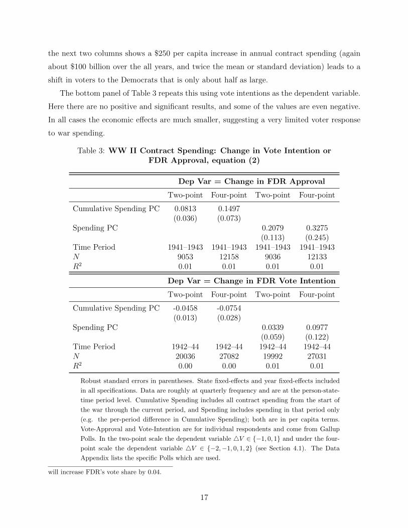
the next two columns shows a $250 per capita increase in annual contract spending (again

about $100 billion over the all years, and twice the mean or standard deviation) leads to a

shift in voters to the Democrats that is only about half as large.

The bottom panel of Table 3 repeats this using vote intentions as the dependent variable.

Here there are no positive and significant results, and some of the values are even negative.

In all cases the economic effects are much smaller, suggesting a very limited voter response

to war spending.

Table 3: WW II Contract Spending: Change in Vote Intention orFDR Approval, equation (2)

Dep Var = Change in FDR Approval

Two-point Four-point Two-point Four-point

Cumulative Spending PC 0.0813 0.1497(0.036) (0.073)

Spending PC 0.2079 0.3275(0.113) (0.245)

Time Period 1941–1943 1941–1943 1941–1943 1941–1943N 9053 12158 9036 12133R2 0.01 0.01 0.01 0.01

Dep Var = Change in FDR Vote Intention


Cumulative Spending PC -0.0458 -0.0754(0.013) (0.028)

Spending PC 0.0339 0.0977(0.059) (0.122)

Time Period 1942–44 1942–44 1942–44 1942–44N 20036 27082 19992 27031R2 0.00 0.00 0.01 0.01

Robust standard errors in parentheses. State fixed-effects and year fixed-effects included

in all specifications. Data are roughly at quarterly frequency and are at the person-state-

time period level. Cumulative Spending includes all contract spending from the start of

the war through the current period, and Spending includes spending in that period only

(e.g. the per-period difference in Cumulative Spending); both are in per capita terms.

Vote-Approval and Vote-Intention are for individual respondents and come from Gallup

Polls. In the two-point scale the dependent variable 4V ∈ {−1, 0, 1} and under the four-

point scale the dependent variable 4V ∈ {−2,−1, 0, 1, 2} (see Section 4.1). The Data

Appendix lists the specific Polls which are used.

will increase FDR’s vote share by 0.04.

17

As a robustness check we considered various modifications of these specifications (and

all two-way permutations of these modifications), and in all cases we continue to find small

economic effects. These include looking at spending in level rather than per capita terms,

using industrial or military spending, using non-differenced voting rather than netting our

previous vote patterns (and estimate using either a linear probability model or a logit), omit-

ting various combinations of fixed effects, including both cumulative and annual spending to

allow for diminishing returns (voters respond primarily to the first increment of spending),

and interacting spending with individual-level demographics such as age, race, religion, par-

ent’s country of origin, urban location, occupation, education, and phone- or car-ownership

(wealth proxies). The latter is especially important since it is a more direct control for

geographic-targeting of funds based on local characteristics.

Table 4 examines New Deal spending over 1936-1940, which might reflect information

politicians had when they started allocating the war spending monies. We repeat the speci-

fications and approach from the previous table. We use the voter’s stated vote in the 1936

presidential election for Vis0, except the very first poll which occurs before that election and

so the vote in 1932 is used there. Except in one case the parameters are not statistically

different from zero, though the standard errors are modest as the sample size is relatively

large. We begin again with voter approval (unlike with the war polls, the voting variables

are evenly spread across the sample period). Using the point estimates and the same model

from the last paragraph, a two hundred and fifty dollar increase in annual spending per

capita increases FDR’s vote share by three and a half to five and a half percent. This is

quite close to the values from war spending. Cumulative spending per capita has a negative

association, with a thousand dollar increase associated with about a one to four percent

reduction in FDR votes. If instead vote intentions are used, the estimates in the final four

columns indicate the effect on FDR votes is about twice as large for annual spending and

about the same (negative) effect for cumulative spending. Echoing the earlier results, there

is little evidence that spending yields large positive shifts in voting, and again the estimates

here are likely upper bound effects.

Overall, there is little support from either the World War II spending or New Deal

spending that votes are especially responsive to government resource allocations. It suggests

that politically strategic allocation of war monies is unlikely to be successful at shaping

electoral outcomes. Still this is just one input in the allocation calculus, and we return to

18

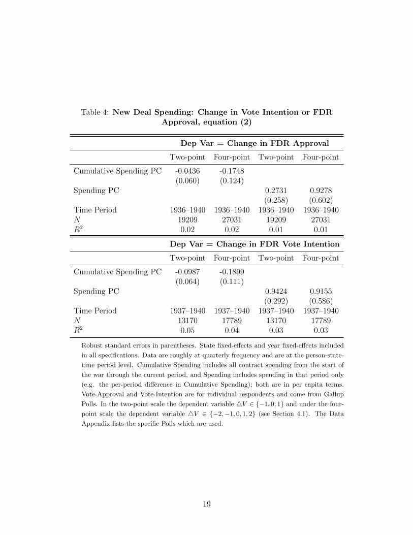
Table 4: New Deal Spending: Change in Vote Intention or FDRApproval, equation (2)

Dep Var = Change in FDR Approval



Spending PC 0.2731 0.9278(0.258) (0.602)

Time Period 1936–1940 1936–1940 1936–1940 1936–1940N 19209 27031 19209 27031R2 0.02 0.02 0.01 0.01

Dep Var = Change in FDR Vote Intention



Spending PC 0.9424 0.9155(0.292) (0.586)

Time Period 1937–1940 1937–1940 1937–1940 1937–1940N 13170 17789 13170 17789R2 0.05 0.04 0.03 0.03

Robust standard errors in parentheses. State fixed-effects and year fixed-effects included

in all specifications. Data are roughly at quarterly frequency and are at the person-state-

time period level. Cumulative Spending includes all contract spending from the start of

the war through the current period, and Spending includes spending in that period only

(e.g. the per-period difference in Cumulative Spending); both are in per capita terms.

Vote-Approval and Vote-Intention are for individual respondents and come from Gallup

Polls. In the two-point scale the dependent variable 4V ∈ {−1, 0, 1} and under the four-

point scale the dependent variable 4V ∈ {−2,−1, 0, 1, 2} (see Section 4.1). The Data

Appendix lists the specific Polls which are used.

19

the importance of politics in the allocation process in the next section.

5 Calculating Pivot Probabilities

Our procedure for estimating the political value, or “pivot probability” of each state in the

1944 presidential election, is similar in spirit to that in Stromberg (2008). The goal is to

answer the following question: For each state i, how likely is it that a marginal change

in supply contract spending state i (either up or down) would change the electoral college

outcome? Note that we focus on the incumbent party’s allocation decision. This is because

it is not clear what assumptions to make regarding voters’ beliefs about what the challenging

Republican party would do in power. The Republicans had not held power nationally for

more than a decade, and had no previous record governing during a crisis similar to WWII

since the Civil War.

First, for each state we calculate the Democratic share of the two party vote in all elections

for U.S. president, U.S. senator, and state governor that took place between 1932 and 1943.7

Denote this by Dijt, where i indexes states, j indexes offices, and t indexes years. Next we

estimate the following model, using OLS:

Dijt = αi + θt + εijt (3)

where αi denotes a vector of state-specific fixed-effects and θt denotes a vector of year-specific

fixed-effects. This yields the “normal Democratic vote” in state i (αi), and the “idiosyncratic

electoral variability” in state i (standard deviation of the residuals for state i). Call these

Dmeani and Dsd

i , respectively. Also, let Ei be the number of votes state i has in the electoral

college, and let Pi be state i’s population.

The next step is to calculate how spending would change vote outcomes, and in turn

whether these changes would alter the election outcome compared to the no spending case.

We must make an assumption about two parameters. The first is the expected national

electoral shock or “national tide” in the 1944, which we denote DN (positive values being in

favor of Democrats and negative values being against).8

7We drop cases in which a third party candidate received more than 15% of the total vote. We also dropcases where the Democratic share of the total vote was less than 5% or greater than 95%. We also ran theanalysis dropping the elections held in 1942 and 1943, and the results are quite similar to those presentedbelow.

8This is akin to the fixed effect θt from the estimates of (3), but those values cannot be used becausethey are for earlier periods.

20

The second is the effect of military spending on the share of votes won by the Democrats

in 1944. As noted above, the standard deviation of contract spending per-capita was about

$1,000, and the average was also about $1,000. The average state population was about

2.7 million. So, we consider changing a state’s total contract spending by $2.7 billion. How

does that translate into votes? This depends on voter behavior—how sensitive voters are

to spending in their state when deciding how to vote—which we denote V m (In order to

avoid parameter values with many decimals, we measure contract spending in thousands of

dollars).9

For each choice of these parameters—discussed shortly—we simulate 10 million elections,

as follows:

(i) Draw an idiosyncratic shock ηi for each state i from a distribution that is N(0, Dsdi ).

(ii) Let Vi = Dmeani +DN + ηi be the Democratic vote share in each state i.

(iii) Calculate the electoral college winner given the vector of Vi’s (there were 531 members

of the electoral college in 1944):

Democratic Win if∑

{i|Vi>.5}

Ei > 265

Republican Win if∑

{i|Vi>.5}

Ei < 265

(iv) In the case of a Republican Win, loop through the set of states with Vi < .5 (the

states won by Republicans) one state at time, and add V m× (2700000/Pi) to Vi while

holding all other states’ voting outcomes fixed. If doing this changes the electoral

college outcome to a Democratic win, then call state i Pivotal .10

In the case of a Democratic Win, loop through the set of states with Vi > .5 (the

states won by Democrats) one state at time, and subtract V m × (2700000/Pi) from Vi

9Note that VM takes on two roles: it measures both vote sensitivity to money and the amount of spending.That is, doubling its value could mean the amount of spending doubles and vote sensitivity stays constant.For our purposes focusing on vote sensitivity is reasonable since we have calibrated the spending level tomatch the actual amount during the war.

10Note that for state i to be pivotal, two changes must occur. First, Vi + V m × (2700000/Pi) mustgreater than .5 (the injection of funds must change the outcome in state i from a Republican majority to aDemocratic majority). Second, state i must have enough electoral college votes so that changing the statefrom Republican to Democratic changes the outcome in the electoral college. The first change will tend tohappen more often in small states, but the second change will tend to happen more often in large states.

21

while holding all other states’ voting outcomes fixed. If doing this changes the electoral

college outcome to a Republican win, then call state i Pivotal .

(v) Let Pivot Probability i be the fraction of times that state i is Pivotal out of the 10 million

simulated elections.

Choosing a range of values for the national tide, DN , is relatively straightforward. The

median presidential vote swing over the period 1920-1944 was about 3%, and historically

swings larger than 5% are relatively rare. To keep things simple we consider three values,

DN = -.03, 0, and .03.

Choosing a range of values for V m is trickier. It should represent the impact of the

overall size of War spending on the Democratic vote share. Our best benchmarks are from

the World War Two and New Deal spending estimates in Section 4. Recall that we consider

two versions of spending (cumulative and per year) as well as four versions of vote change

(omitting and including previous non-voters, and vote intention versus vote approval). As

discussed in that section, in each case we can convert the parameter values into the change in

Democratic vote share from total war spending.11 For the World War Two spending (Table 3)

the average imputed V M value is 0.012 with a maximum of 0.041. For New Deal spending

(Table 4) the average is 0.013 and the maximum is 0.118. In addition, when V m = .0621801,

the average vote shift caused by military spending is equal to the average (across states)

of the within-state standard deviation of vote share across years and offices. We examine a

range of possible V M , but we think the most plausible value is around 0.05 or 0.06 (since

some of the underlying parameter estimates are negative).

We consider V m ∈ {.03, .06, .09, .12, .15, .18, .21, .24, .27, .30}. We include the high

values in our analyses to show what the model would predict if politicians believed that

military spending was highly effective at winning votes.

We ran 30 separate simulations, one for each combination of DN (×3) and V m (×10).

11The spending parameters, like VM , are denominated in thousands of dollars per capita. The parameterthen must be divided by certain factors depending on the combination of spending and vote variable beingused. For cumulative spending roughly a thousand dollars matches the overall war total (F1 = 1) while forper year spending the amount is two hundred and fifty dollars (F1 = 4). For the vote scale the values shouldbe mapped into the unit interval to give vote shares which can be applied to the two-point (F2 = 2) andfour-point (F2 = 4) scales. Finally, to convert to expected voting we use a common factor for vote intentionsand vote approval (F3 = 1). The vote approval factor in principle could differ (since it is not literally how anindividual plans to vote), but using data from OPOR surveys and regressing vote intention on vote approvalshows that for the observed range of approval values that little adjustment is needed (regression available

upon request). So to map the parameter estimate into a fitted VM value we take β/(F1 × F2 × F3).

22

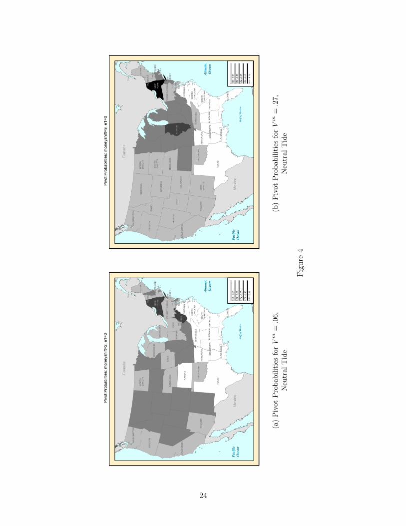
Figures 4a and 4b show how the pivot probabilities vary across states, for two values of

V m—.09 (a “reasonable” value), and .27 (probably implausibly large).

The graphs suggest that the pivotal probabilities are plausible, and also that they pro-

vide value added over other approaches. While the probabilities vary with V m and DN ,

the ordering of the states is relatively stable. States with high pivot probabilities—such as

New York, Illinois, and Missouri—are those which are not strongly aligned with one party,

while those with pivot probabilities of zero—South Carolina, Mississippi, Louisiana, Georgia,

Alabama—tilt heavily towards Democrats. In fact, the states of the solid south are essen-

tially never pivotal. The results also differ from simpler and more naive approaches. For

example one could see which states have the most volatile historical votes. This would be an

unsatisfactory measure since it ignores both the the baseline partisanship of the state and

the state’s size. In fact historical volatility has little correlation with any of the state-level

pivotal probability measures (results available upon request).12

12Volatility is the residual standard error from (3).

23

(a)

Piv

otP

rob

abil

itie

sfo

rV

m=.0

6,N

eutr

alT

ide

(b)

Piv

otP

rob

abil

itie

sfo

rV

m=.2

7,

Neu

tral

Tid

e

Fig

ure

4

24

6 Results

This section presents the main estimates explaining the spatial distribution of spending

across states. The focus is on determining the relative contributions of political and economic

efficiency mechanisms. We begin with a short motivational approach which gives preliminary

evidence of the limited role of political factors. The second sub-section presents the formal

estimates.

6.1 Motivation

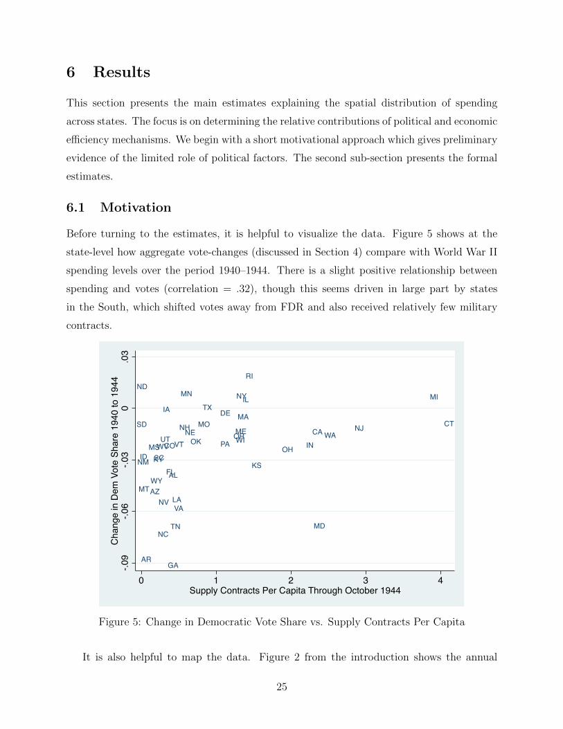
Before turning to the estimates, it is helpful to visualize the data. Figure 5 shows at the

state-level how aggregate vote-changes (discussed in Section 4) compare with World War II

spending levels over the period 1940–1944. There is a slight positive relationship between

spending and votes (correlation = .32), though this seems driven in large part by states

in the South, which shifted votes away from FDR and also received relatively few military

contracts.

AL

AR

AZ

CA

CO

CTDE

FL

GA

IA

ID

IL

IN

KSKY

LA

MA

MD

ME

MIMN

MO

MS

MT

NC

ND

NENH NJ

NM

NV

NY

OHOK OR

PA

RI

SC

SD

TN

TX

UT

VA

VTWAWI

WV

WY

-.09

-.06

-.03

0.0

3Ch

ange

in D

em V

ote

Shar

e 19

40 to

194

4

0 1 2 3 4Supply Contracts Per Capita Through October 1944

Figure 5: Change in Democratic Vote Share vs. Supply Contracts Per Capita

It is also helpful to map the data. Figure 2 from the introduction shows the annual

25

allocation of per capita contract spending across states. Spending is heavily concentrated in

the Northeast, Industrial Midwest, and West Coast. It is also relatively stable over time, with

these states getting the highest spending in the peak years (19421-1944) as well as the lower

spending years at the beginning and end (1940-1941 and 1945). While this such consistency

could reflect political factors, other explanations seem more relevant. Economic efficiency is

likely playing a role in the allocation since the high spending states have significant industrial

capacity and shipyards. It is also important to note that other regions receive substantial

spending. In particular the South, which is the least pivotal region (Figure 4), has significant

spending, in opposition to what would be expected from politically motivated allocation.

Figure 6 shows the temporal pattern of aggregate national spending per capita and voter

support for FDR during the period between the 1940 and 1944 elections. Spending was

highest at the onset of the war in 1942, and slows down substantially just before the 1944

election. This is inconsistent with the strategic allocation of spending for two reasons. First,

it is the period just before the election when many voters make their final choice between

candidates and so spending would be most efficient at this time in gaining votes. Second,

spending is smallest during the periods when FDR was most vulnerable to not getting re-

elected and so political-based allocation would be most attractive (spending changes slightly

lag approval changes, but they reinforce rather than offset political support). Comparing the

two series, we see spending and approval move in a similar fashion—in fact, the correlation

coefficient is 0.80 for the two series. Both series surge following the attack on Pearl Harbor—

with FDR approval rising first—and then both dissipate and largely bottom out in the

months leading up to the 1944 election. So long as these swings in voter support were

largely driven by external factors such as patriotic response to the initiation of the War, this

suggests political strategy was not central to the timing of war spending which would have

been more beneficial in the later years where FDR’s support had diminished.

6.2 Estimates

We estimated the following model, using OLS:

Spending i = β0 + β1Pivot Probability i + β2Total Manuf i + β3Aircraft Manuf i + εi (4)

We estimated the model for each of the Spending i variables described above, and for each of

the 30 separate Pivot Probability vectors, which represent the role of political factors. The

Manuf covariates are measures of manufacturing capacity and capture the role of economic

26

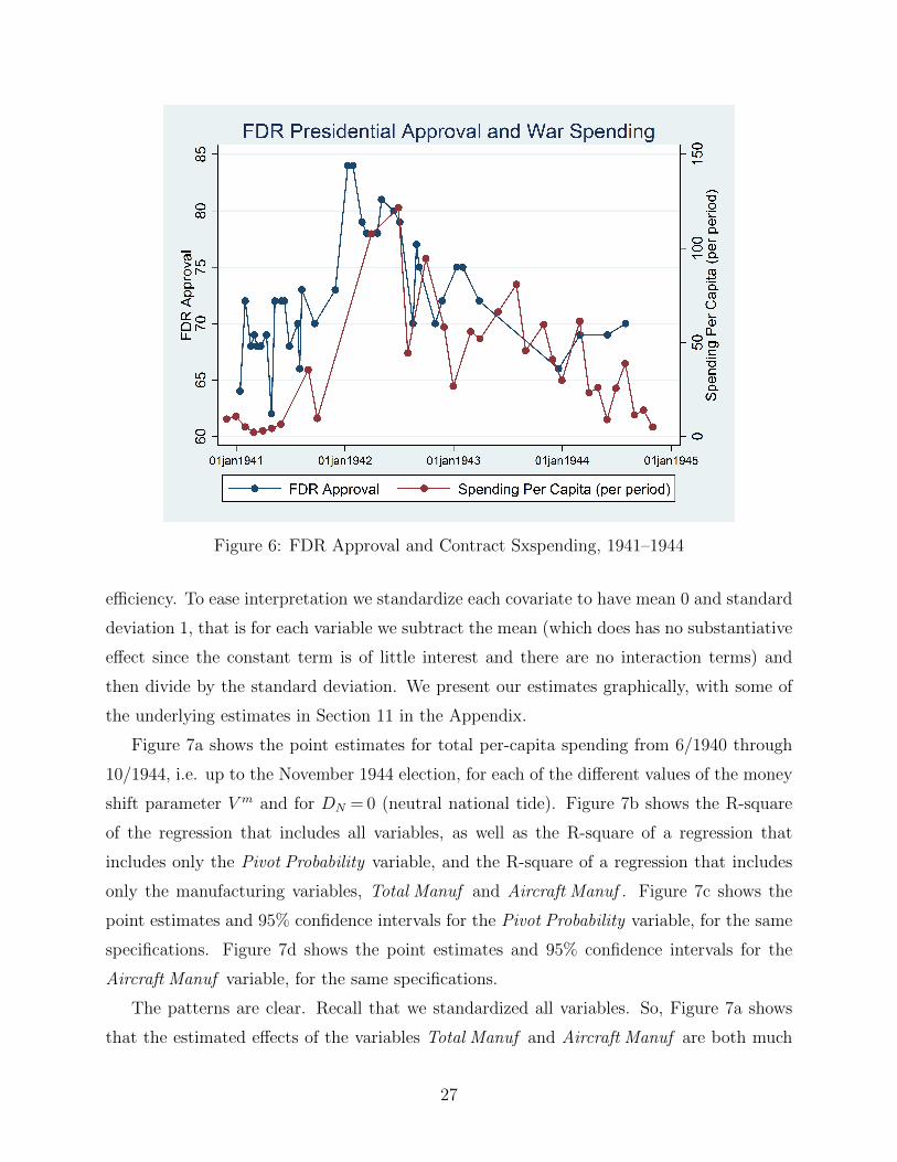
Figure 6: FDR Approval and Contract Sxspending, 1941–1944

efficiency. To ease interpretation we standardize each covariate to have mean 0 and standard

deviation 1, that is for each variable we subtract the mean (which does has no substantiative

effect since the constant term is of little interest and there are no interaction terms) and

then divide by the standard deviation. We present our estimates graphically, with some of

the underlying estimates in Section 11 in the Appendix.

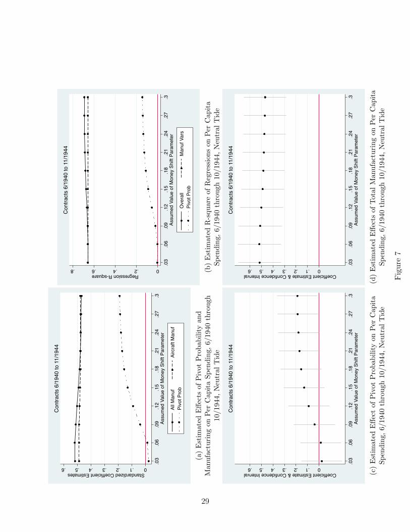
Figure 7a shows the point estimates for total per-capita spending from 6/1940 through

10/1944, i.e. up to the November 1944 election, for each of the different values of the money

shift parameter V m and for DN = 0 (neutral national tide). Figure 7b shows the R-square

of the regression that includes all variables, as well as the R-square of a regression that

includes only the Pivot Probability variable, and the R-square of a regression that includes

only the manufacturing variables, Total Manuf and Aircraft Manuf . Figure 7c shows the

point estimates and 95% confidence intervals for the Pivot Probability variable, for the same

specifications. Figure 7d shows the point estimates and 95% confidence intervals for the

Aircraft Manuf variable, for the same specifications.

The patterns are clear. Recall that we standardized all variables. So, Figure 7a shows

that the estimated effects of the variables Total Manuf and Aircraft Manuf are both much

27

higher than the estimated effect of the Pivot Probability variable, for all values of V m. Figure

7b shows that the variables Total Manuf and Aircraft Manuf account for almost all of the

regression R-square, and the contribution of Pivot Probability is minimal. Figure 7c shows

that the estimated effect of Pivot Probability is not even statistically significant at the .05

level, except for very large values of Vm, values of 8 or higher. By contrast, Figure 7d shows

that the estimated effect of Total Manuf is always highly significant at the .05 level.

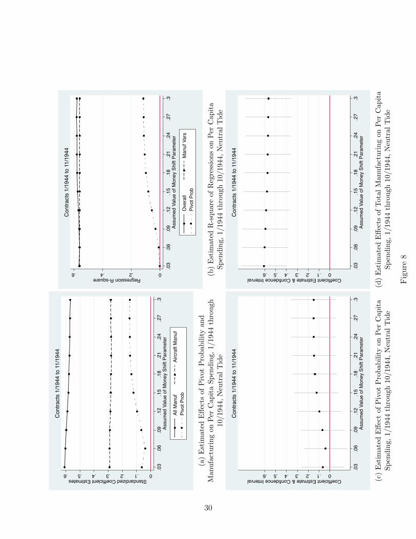
It is possible that although overall spending was not clearly targeted at pivotal states,

spending closer to the election of 1944 was. In fact, this is not the case.13 Figures 8a-8d are

analogous to Figures 7a-7d, but the dependent variable is for contract spending only in 1944

(January through October). The overall patterns are quite similar: the estimated effects of

the Total Manuf variable is much higher than the estimated effect of the Pivot Probability

variable (though this is not longer the case for the Aircraft Manuf variable); the variables

Total Manuf and Aircraft Manuf account for almost all of the regression R-square, and the

contribution of Pivot Probability is minimal; the estimated effect of Pivot Probability is never

statistically significant at the .05 level, even for the highest values of Vm; and the estimated

effect of Total Manuf is always highly significant at the .05 level.

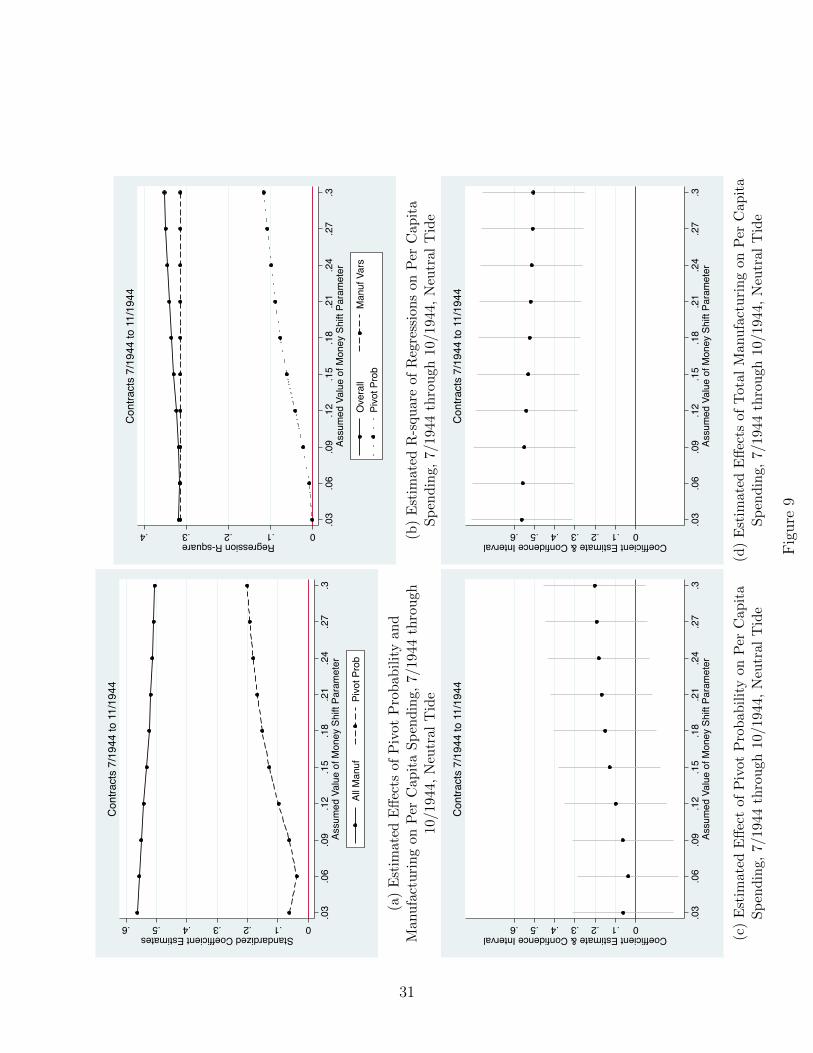
Figures 9a-9d zero in even closer to the election, examining the distribution of contract

spending in the four months just prior to the election—July through 10/1944.14 The bottom

line is again the same. There is little evidence that contracts were allocated disproportion-

ately towards pivotal states.15

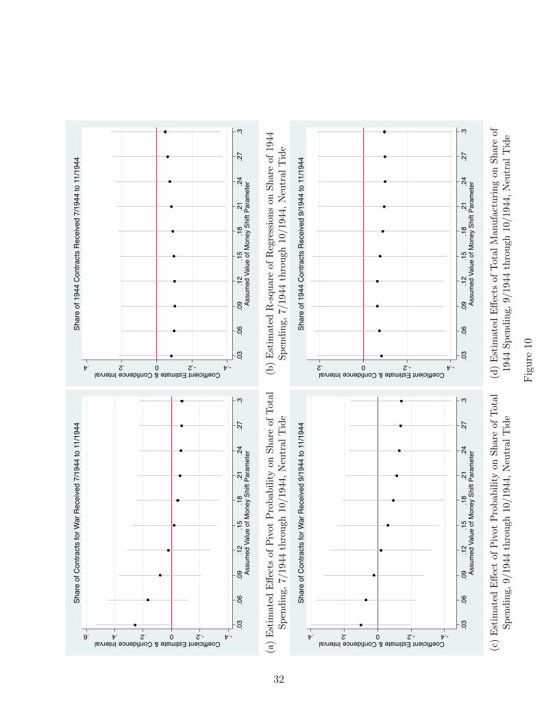
Finally, Figures 10a-10d search for evidence of electorally-related targeting from a slightly

different point of view, by studying the share of money spent in a state during the 2 or 4

months prior to the election, as a percentage of the total amount of money spent in the state

over the whole war, or over the whole year 1944. In all figures we focus on the estimated

coefficient and standard error of Pivot Probability . Figures 10a and 10b consider the 4-month

period leading up to the November 1944 election (July through October), while figures 10c

and 10d consider an even shorter 2-month period (September through October). In all cases

the bottom line is the same: the estimated effect of Pivot Probability on the share of money

spent during the election campaign is never statistically distinguishable from zero.

13As further evidence, recall from Figure 1 that little spending occurs right before the election.14In these regressions we drop the Aircraft Manuf variable.15Other intervals, two, three, or five months leading up the election exhibit similar patterns.

28

0.1.2.3.4.5.6Standardized Coefficient Estimates

.03

.06

.09

.12

.15

.18

.21

.24

.27

.3As

sum

ed V

alue

of M

oney

Shi

ft Pa

ram

eter

All M

anuf

Airc

raft

Man

ufPi

vot P

rob

Con

tract

s 6/

1940

to 1

1/19

44

(a)

Est

imat

edE

ffec

tsof

Piv

otP

rob

abil

ity

and

Man

ufa

ctu

rin

gon

Per

Cap

ita

Sp

end

ing,

6/19

40th

rou

gh10

/194

4,N

eutr

alT

ide

0.2.4.6.8Regression R-square

.03

.06

.09

.12

.15

.18

.21

.24

.27

.3As

sum

ed V

alue

of M

oney

Shi

ft Pa

ram

eter

Ove

rall

Man

uf V

ars

Pivo

t Pro

b

Cont

ract

s 6/

1940

to 1

1/19

44

(b)

Est

imat

edR

-squ

are

ofR

egre

ssio

ns

on

Per

Capit

aS

pen

din

g,6/

1940

thro

ugh

10/1

944,

Neu

tral

Tid

e

0.1.2.3.4.5.6Coefficient Estimate & Confidence Interval

.03

.06

.09

.12

.15

.18

.21

.24

.27

.3As

sum

ed V

alue

of M

oney

Shi

ft Pa

ram

eter

Con

tract

s 6/

1940

to 1

1/19

44

(c)

Est

imat

edE

ffec

tof

Piv

otP

rob

abil

ity

onP

erC

apit

aS

pen

din

g,6/

1940

thro

ugh

10/1

944,

Neu

tral

Tid

e


.03

.06

.09

.12

.15

.18

.21

.24

.27

.3As

sum

ed V

alue

of M

oney

Shi

ft Pa

ram

eter

Con

tract

s 6/

1940

to 1

1/19

44

(d)

Est

imat

edE

ffec

tsof

Tot

alM

anu

fact

uri

ng

on

Per

Cap

ita

Sp

end

ing,

6/19

40th

rou

gh10

/194

4,

Neu

tral

Tid

e

Fig

ure

7

29


.03

.06

.09

.12

.15

.18

.21

.24

.27

.3As

sum

ed V

alue

of M

oney

Shi

ft Pa

ram

eter

All M

anuf

Airc

raft

Man

ufPi

vot P

rob

Con

tract

s 1/

1944

to 1

1/19

44

(a)

Est

imat

edE

ffec

tsof

Piv

otP

rob

abil

ity

and

Man

ufa

ctu

rin

gon

Per

Cap

ita

Sp

end

ing,

1/19

44th

rou

gh10

/194

4,N

eutr

alT

ide

0.2.4.6Regression R-square

.03

.06

.09

.12

.15

.18

.21

.24

.27

.3As

sum

ed V

alue

of M

oney

Shi

ft Pa

ram

eter

Ove

rall

Man

uf V

ars

Pivo

t Pro

b

Cont

ract

s 1/

1944

to 1

1/19

44

(b)

Est

imat

edR

-squ

are

ofR

egre

ssio

ns

on

Per

Capit

aS

pen

din

g,1/

1944

thro

ugh

10/1

944,

Neu

tral

Tid

e


.03

.06

.09

.12

.15

.18

.21

.24

.27

.3As

sum

ed V

alue

of M

oney

Shi

ft Pa

ram

eter

Con

tract

s 1/

1944

to 1

1/19

44

(c)

Est

imat

edE

ffec

tof

Piv

otP

rob

abil

ity

onP

erC

apit

aS

pen

din

g,1/

1944

thro

ugh

10/1

944,

Neu

tral

Tid

e


.03

.06

.09

.12

.15

.18

.21

.24

.27

.3As

sum

ed V

alue

of M

oney

Shi

ft Pa

ram

eter

Con

tract

s 1/

1944

to 1

1/19

44

(d)

Est

imat

edE

ffec

tsof

Tot

alM

anu

fact

uri

ng

on

Per

Cap

ita

Sp

end

ing,

1/19

44th

rou

gh10

/194

4,

Neu

tral

Tid

e

Fig

ure

8

30


.03

.06

.09

.12

.15

.18

.21

.24

.27

.3As

sum

ed V

alue

of M

oney

Shi

ft Pa

ram

eter

All M

anuf

Pivo

t Pro

b

Con

tract

s 7/

1944

to 1

1/19

44

(a)

Est

imat

edE

ffec

tsof

Piv

otP

rob

abil

ity

and

Man

ufa

ctu

rin

gon

Per

Cap

ita

Sp

end

ing,

7/19

44th

rou

gh10

/194

4,N

eutr

alT

ide

0.1.2.3.4Regression R-square

.03

.06

.09

.12

.15

.18

.21

.24

.27

.3As

sum

ed V

alue

of M

oney

Shi

ft Pa

ram

eter

Ove

rall

Man

uf V

ars

Pivo

t Pro

b

Cont

ract

s 7/

1944

to 1

1/19

44

(b)

Est

imat

edR

-squ

are

ofR

egre

ssio

ns

on

Per

Capit

aS

pen

din

g,7/

1944

thro

ugh

10/1

944,

Neu

tral

Tid

e


.03

.06

.09

.12

.15

.18

.21

.24

.27

.3As

sum

ed V

alue

of M

oney

Shi

ft Pa

ram

eter

Con

tract

s 7/

1944

to 1

1/19

44

(c)

Est

imat

edE

ffec

tof

Piv

otP

rob

abil

ity

onP

erC

apit

aS

pen

din

g,7/

1944

thro

ugh

10/1

944,

Neu

tral

Tid

e


.03

.06

.09

.12

.15

.18

.21

.24

.27

.3As

sum

ed V

alue

of M

oney

Shi

ft Pa

ram

eter

Con

tract

s 7/

1944

to 1

1/19

44

(d)

Est

imat

edE

ffec

tsof

Tot

alM

anu

fact

uri

ng

on

Per

Cap

ita

Sp

end

ing,

7/19

44th

rou

gh10

/194

4,

Neu

tral

Tid

e

Fig

ure

9

31

-.4-.20.2.4.6Coefficient Estimate & Confidence Interval

.03

.06

.09

.12

.15

.18

.21

.24

.27

.3As

sum

ed V

alue

of M

oney

Shi

ft Pa

ram

eter

Shar

e of

Con

tract

s fo

r War

Rec

eive

d 7/

1944

to 1

1/19

44

(a)

Est

imat

edE

ffec

tsof

Piv

otP

rob

abil

ity

onS

har

eof

Tot

alS

pen

din

g,7/

1944

thro

ugh

10/1

944,

Neu

tral

Tid

e

-.4-.20.2.4Coefficient Estimate & Confidence Interval

.03

.06

.09

.12

.15

.18

.21

.24

.27

.3As

sum

ed V

alue

of M

oney

Shi

ft Pa

ram

eter

Shar

e of

194

4 C

ontra

cts

Rec

eive

d 7/

1944

to 1

1/19

44

(b)

Est

imat

edR

-squ

are

ofR

egre

ssio

ns

on

Sh

are

of

1944

Sp

end

ing,

7/19

44th

rou

gh10

/194

4,

Neu

tral

Tid

e

-.4-.20.2.4Coefficient Estimate & Confidence Interval

.03

.06

.09

.12

.15

.18

.21

.24

.27

.3As

sum

ed V

alue

of M

oney

Shi

ft Pa

ram

eter

Shar

e of

Con

tract

s fo

r War

Rec

eive

d 9/

1944

to 1

1/19

44

(c)

Est

imat

edE

ffec

tof

Piv

otP

rob

abil

ity

onS

har

eof

Tot

alS

pen

din

g,9/

1944

thro

ugh

10/1

944,

Neu

tral

Tid

e

-.4-.20.2Coefficient Estimate & Confidence Interval

.03

.06

.09

.12

.15

.18

.21

.24

.27

.3As

sum

ed V

alue

of M

oney

Shi

ft Pa

ram

eter

Shar

e of

194

4 C

ontra

cts

Rec

eive

d 9/

1944

to 1

1/19

44

(d)

Est

imat

edE

ffec

tsof

Tot

alM

anu

fact

uri

ng

on

Sh

are

of

1944

Sp

end

ing,

9/19

44th

rou

gh10

/1944,

Neu

tral

Tid

e

Fig

ure

10

32

7 Robustness Checks

In this section we consider some empirical extensions. We consider whether money is allo-

cated based on Congressional seniority or whether there are specific patterns to one specific

kind of spending, facilities spending. We continue not to find strong evidence for the role of

politics in either of these cases.

7.1 Congressional Seniority

While not the focus of this paper, we also ran specifications that include variables to check for

congressional influence over the distribution of spending. More specifically, we constructed

several indices of “institutional power” for each state and checked whether states with more

powerful delegations received contract dollars. To construct the indices we use the follow-

ing House and Senate positions: Speaker of the House, Majority Leader, Minority Leader,

member of the House Ways and Means committee, member of the House Appropriations

committee, member of the House Rules committee, member of the Senate Finance commit-

tee, member of the Senate Appropriations committee, member of the House Military Affairs

committee, member of the House Naval Affairs committee, member of the Senate Military

Affairs committee, and member of the Senate Naval Affairs committee. Let HS be the set of

all of these positions, let H be the set of all positions from the House, let S be the set of all

positions from the Senate, and let M be the set of the four positions involving defense-related

committees plus the two Appropriations committees.

The broadest index, which we denote House and Senate Overall Power , is constructed as

follows: For each state i count the total number of positions in the set HS held by the state’s

House and Senate delegation in year t. The chamber-specific indices, House Overall Power

and Senate Overall Power are constructed similarly but each index considers only the po-

sitions in H and S, respectively. Finally, the more jurisdiction-specific index, House and

Senate Military Power is constructed by counting only those positions in M . For each index

we then divide by state population. Note that the indices will therefore reflect the Senate

malapportionment that gives small states more representation per person than large states.

We present the estimates of interest in Table 5. The bottom line from the regression

results is simple. None of these variables is statistically significant in any specification, the

point estimates are more often negative than positive (all of the point estimates in Table 5 are

negative), and in all cases the point estimates are substantively small. Importantly, including

33

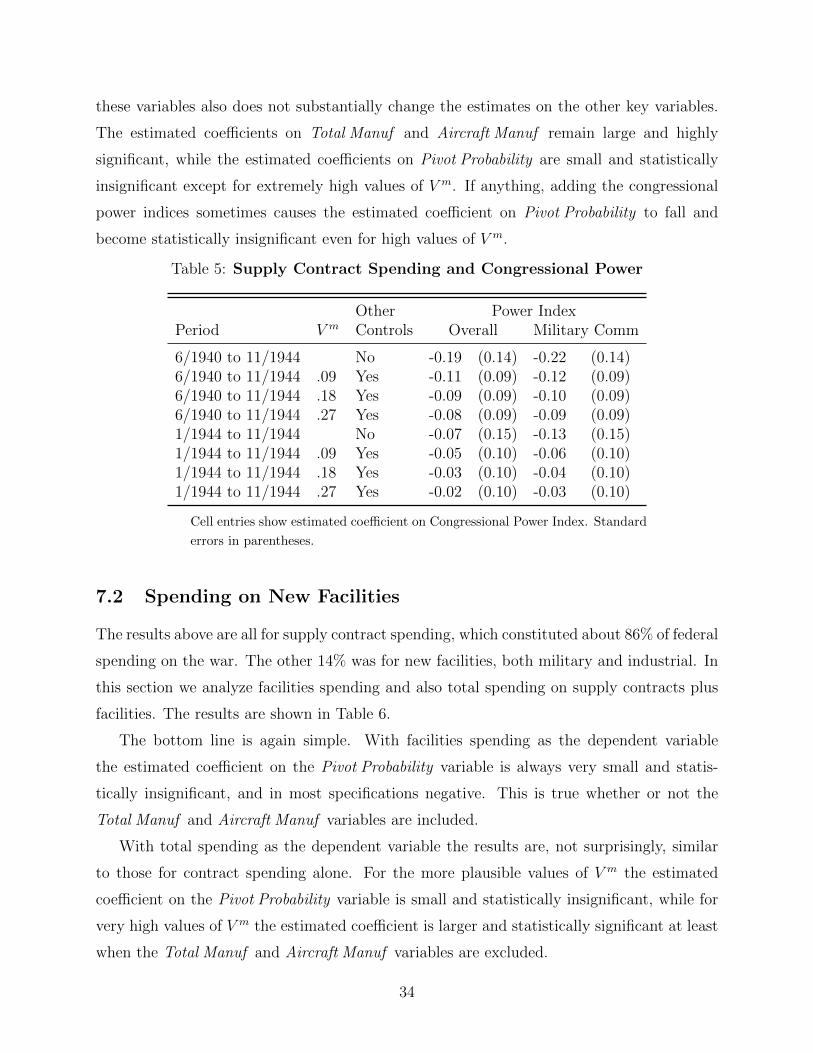
these variables also does not substantially change the estimates on the other key variables.

The estimated coefficients on Total Manuf and Aircraft Manuf remain large and highly

significant, while the estimated coefficients on Pivot Probability are small and statistically

insignificant except for extremely high values of V m. If anything, adding the congressional

power indices sometimes causes the estimated coefficient on Pivot Probability to fall and

become statistically insignificant even for high values of V m.

Table 5: Supply Contract Spending and Congressional Power

Other Power IndexPeriod V m Controls Overall Military Comm

6/1940 to 11/1944 No -0.19 (0.14) -0.22 (0.14)6/1940 to 11/1944 .09 Yes -0.11 (0.09) -0.12 (0.09)6/1940 to 11/1944 .18 Yes -0.09 (0.09) -0.10 (0.09)6/1940 to 11/1944 .27 Yes -0.08 (0.09) -0.09 (0.09)1/1944 to 11/1944 No -0.07 (0.15) -0.13 (0.15)1/1944 to 11/1944 .09 Yes -0.05 (0.10) -0.06 (0.10)1/1944 to 11/1944 .18 Yes -0.03 (0.10) -0.04 (0.10)1/1944 to 11/1944 .27 Yes -0.02 (0.10) -0.03 (0.10)

Cell entries show estimated coefficient on Congressional Power Index. Standard

errors in parentheses.

7.2 Spending on New Facilities

The results above are all for supply contract spending, which constituted about 86% of federal

spending on the war. The other 14% was for new facilities, both military and industrial. In

this section we analyze facilities spending and also total spending on supply contracts plus

facilities. The results are shown in Table 6.

The bottom line is again simple. With facilities spending as the dependent variable

the estimated coefficient on the Pivot Probability variable is always very small and statis-

tically insignificant, and in most specifications negative. This is true whether or not the

Total Manuf and Aircraft Manuf variables are included.

With total spending as the dependent variable the results are, not surprisingly, similar

to those for contract spending alone. For the more plausible values of V m the estimated

coefficient on the Pivot Probability variable is small and statistically insignificant, while for

very high values of V m the estimated coefficient is larger and statistically significant at least

when the Total Manuf and Aircraft Manuf variables are excluded.

34

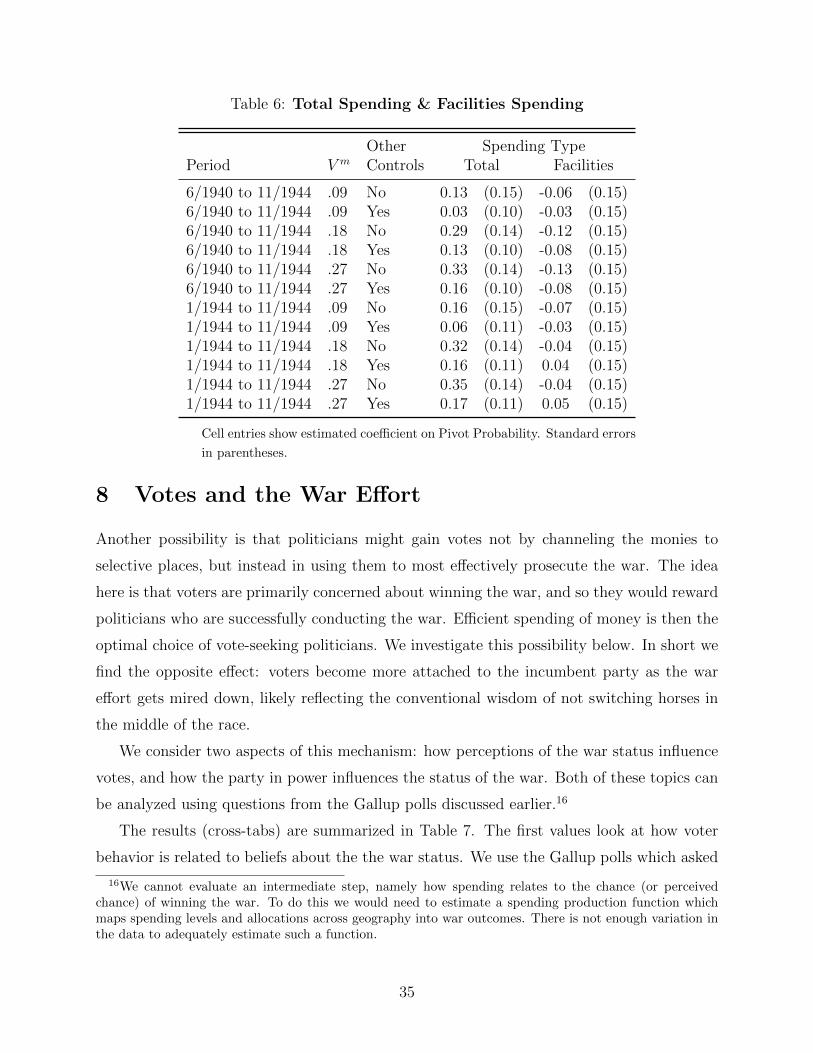
Table 6: Total Spending & Facilities Spending

Other Spending TypePeriod V m Controls Total Facilities

6/1940 to 11/1944 .09 No 0.13 (0.15) -0.06 (0.15)6/1940 to 11/1944 .09 Yes 0.03 (0.10) -0.03 (0.15)6/1940 to 11/1944 .18 No 0.29 (0.14) -0.12 (0.15)6/1940 to 11/1944 .18 Yes 0.13 (0.10) -0.08 (0.15)6/1940 to 11/1944 .27 No 0.33 (0.14) -0.13 (0.15)6/1940 to 11/1944 .27 Yes 0.16 (0.10) -0.08 (0.15)1/1944 to 11/1944 .09 No 0.16 (0.15) -0.07 (0.15)1/1944 to 11/1944 .09 Yes 0.06 (0.11) -0.03 (0.15)1/1944 to 11/1944 .18 No 0.32 (0.14) -0.04 (0.15)1/1944 to 11/1944 .18 Yes 0.16 (0.11) 0.04 (0.15)1/1944 to 11/1944 .27 No 0.35 (0.14) -0.04 (0.15)1/1944 to 11/1944 .27 Yes 0.17 (0.11) 0.05 (0.15)

Cell entries show estimated coefficient on Pivot Probability. Standard errors

in parentheses.

8 Votes and the War Effort

Another possibility is that politicians might gain votes not by channeling the monies to

selective places, but instead in using them to most effectively prosecute the war. The idea

here is that voters are primarily concerned about winning the war, and so they would reward

politicians who are successfully conducting the war. Efficient spending of money is then the

optimal choice of vote-seeking politicians. We investigate this possibility below. In short we

find the opposite effect: voters become more attached to the incumbent party as the war

effort gets mired down, likely reflecting the conventional wisdom of not switching horses in

the middle of the race.

We consider two aspects of this mechanism: how perceptions of the war status influence

votes, and how the party in power influences the status of the war. Both of these topics can

be analyzed using questions from the Gallup polls discussed earlier.16

The results (cross-tabs) are summarized in Table 7. The first values look at how voter

behavior is related to beliefs about the the war status. We use the Gallup polls which asked

16We cannot evaluate an intermediate step, namely how spending relates to the chance (or perceivedchance) of winning the war. To do this we would need to estimate a spending production function whichmaps spending levels and allocations across geography into war outcomes. There is not enough variation inthe data to adequately estimate such a function.

35

voters how they would vote conditional on the war continuing and on the war ending. The

bottom two panels show that having the war persist leads about 10-15% of voters to shift

to Democrats relative to how they would vote if the war was to end. In addition a heavy

majority of voters do not change their voting based on the war status, and that these effects

are comparable for those who voted Democrat or who Republican in the 1940 election.

One challenge of interpreting these estimates is that there are two reasons that the war

status could influence voter support for the president. There is the usual idea of that voters

prefer continuity in their politicians so long as the war is continuing, and are more open

to a change in peace time. But if the war continues for a while that might also mean the

president is doing a poor job fighting the war. We explore this second possibility next by

examining whether voters believe switching parties will lead the war to be wind down faster.

Table 8 presents results on how voters believe the party in power will influence how

quickly the war will be prosecuted. Voters believe Republicans will be slower at ending the

war, and this tilt becomes more prominent as we approach the 1944 election. Still about

half of all voters believe the party in power has no effect on how quickly the war will be

completed, and there are clear partisan differences with prior Democrat voters being far more

skeptical of the efficacy of Republicans. But more importantly the conclusion is that voters

believe a Democrat government will more quickly end the war, so they seem to comfortable

in how FDR’s performance.17

9 Conclusion

The bottom line from our analysis is straightforward. First, we find evidence consistent with

the hypothesis that supply contracts during WWII were awarded to states that had high

industrial capacity already in place in 1939—most likely, states with industrial plants that

could be modified relatively quickly and cheaply to produce needed war supplies. Second,

we do not find consistent evidence that supply contracts were awarded to states that were

especially likely to be pivotal in the 1944 presidential election. Thus, the evidence suggests

17Further support for this comes from The Office of Public Opinion Research (OPOR) which ran a numberof surveys during the war. One survey (No. 6) conducted April 2-7, 1943 included questions on whetherthe individual would support FDR for a fourth term if the war were over, whether he or she recalled votingfor Roosevelt (vs. Willkie) in 1940, and whether the United States was doing all it possibly can to win thewar. Even after controlling for backing Roosevelt in 1940, there was a positive and statistically significantrelationship between reporting the United States was strong and supporting a fourth term if the war wasover (regression omitted).

36

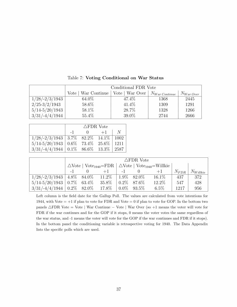
Table 7: Voting Conditional on War Status

Conditional FDR VoteVote | War Continue Vote | War Over NWar Continue NWar Over

1/28/-2/3/1943 64.0% 47.4% 1368 24452/25-3/2/1943 58.6% 41.4% 1309 12915/14-5/20/1943 58.1% 28.7% 1328 12663/31/-4/4/1944 55.4% 39.0% 2744 2666

4FDR Vote-1 0 +1 N

1/28/-2/3/1943 3.7% 82.2% 14.1% 10025/14-5/20/1943 0.6% 73.4% 25.6% 12113/31/-4/4/1944 0.1% 86.6% 13.3% 2587

4FDR Vote4Vote | Vote1940=FDR 4Vote | Vote1940=Willkie

-1 0 +1 -1 0 +1 NFDR NWillkie

1/28/-2/3/1943 4.8% 84.0% 11.2% 1.9% 82.0% 16.1% 437 3725/14-5/20/1943 0.7% 63.4% 35.8% 0.2% 87.6% 12.2% 547 4283/31/-4/4/1944 0.2% 82.0% 17.8% 0.0% 93.5% 6.5% 1217 956

Left column is the field date for the Gallup Poll. The values are calculated from vote intentions for

1944, with Vote = +1 if plan to vote for FDR and Vote = 0 if plan to vote for GOP. In the bottom two

panels 4FDR Vote = Vote | War Continue − Vote | War Over (so +1 means the voter will vote for

FDR if the war continues and for the GOP if it stops, 0 means the voter votes the same regardless of

the war status, and -1 means the voter will vote for the GOP if the war continues and FDR if it stops).

In the bottom panel the conditioning variable is retrospective voting for 1940. The Data Appendix

lists the specific polls which are used.

37

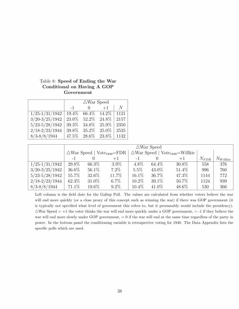
Table 8: Speed of Ending the WarConditional on Having A GOP

Government

4War Speed-1 0 +1 N

1/25-1/31/1942 19.4% 66.4% 14.2% 11213/20-3/25/1942 23.0% 52.2% 24.8% 21575/23-5/28/1942 39.3% 34.8% 25.9% 23502/18-2/23/1944 39.8% 35.2% 25.0% 25358/3-8/8/1944 47.5% 28.6% 23.8% 1132

4War Speed4War Speed | Vote1940=FDR 4War Speed | Vote1940=Willkie

-1 0 +1 -1 0 +1 NFDR NWillkie

1/25-1/31/1942 29.8% 66.3% 3.9% 4.8% 64.4% 30.8% 558 3763/20-3/25/1942 36.6% 56.1% 7.2% 5.5% 43.0% 51.4% 996 7605/23-5/28/1942 55.7% 32.6% 11.7% 16.1% 36.7% 47.3% 1144 7722/18-2/23/1944 62.3% 31.0% 6.7% 10.2% 39.1% 50.7% 1124 9398/3-8/8/1944 71.1% 19.6% 9.2% 10.4% 41.0% 48.6% 530 366

Left column is the field date for the Gallup Poll. The values are calculated from whether voters believe the war

will end more quickly (or a close proxy of this concept such as winning the war) if there was GOP government (it

is typically not specified what level of government this refers to, but it presumably would include the presidency).

4War Speed = +1 the voter thinks the war will end more quickly under a GOP government, = -1 if they believe the

war will end more slowly under GOP government, = 0 if the war will end at the same time regardless of the party in

power. In the bottom panel the conditioning variable is retrospective voting for 1940. The Data Appendix lists the

specific polls which are used.

38

that the distribution of supply contracts was driven more by practical concerns than by

purely political calculations.

It is possible that other political factors were at play, including inter-party competition

for control of Congress, or the re-election concerns of individual congressional incumbents.

Members of key House and Senate committees, or senior members, including committee

and subcommittee chairs, might have sought to steer spending towards their states and

districts. A careful investigation of these hypotheses requires more fine-grained data that

can be mapped into congressional districts, and we leave this for future work.

39

References

Battaglini, Marco and Stephen Coate. 2008. “A Dynamic Theory of Public Spending, Tax-

ation, and Debt.” American Economic Review 98(1):201–36.

Becker, Gary S. 1983. “A Theory of Competition Among Pressure Groups for Political

Influence.” Quarterly Journal of Economics 98(3):371–400.

Brams, Steven J. and Morton D. Davis. 1974. “The 3/2’s Rule in Presidential Campaigning.”

The American Political Science Review 68(1):113–134.

Brams, Steven J. and Morton D. Davis. 1982. “Optimal Resource Allocation in Presidential

Primaries.” Mathematical Social Sciences 3:373–288.

Cardona, Daniel and Antoni Rubı-Barcelo. 2013. On the Optimality of Bargaining Outcomes

in the Collective-Particularistic Multilateral Bargaining Game. DEA Working Papers 53

Universitat de les Illes Balears, Departament d’Economa Aplicada.

Colantoni, Claude S., Terrence J. Levesque and Peter C. Ordeshook. 1975. “Campaign

Resource Allocations Under the Electoral College.” The American Political Science Review

69(1):141–154.

Hudak, John. 2014. The Politics of Federal Grants: Presidential Influence over the Distri-

bution of Federal Funds. Washington DC: Brookings Institution Press.

Leblanc, William, James M. Snyder, Jr. and Micky Tripathi. 2000. “Majority-rule Bargain-

ing and the Under Provision of Public Investment Goods.” Journal of Public Economics

75(1):21–47.

Lindbeck, Assar and Jorgen W. Weibull. 1987. “Balanced-Budget Redistribution as the

Outcome of Political Competition.” Public Choice 52(3):273–297.

Lizzeri, Allesando and Nicola Persico. 2005. “A Drawback of Electoral Competition.” Journal

of the European Economic Association 3:1318–1348.

McCarty, Nolan M. 2000. “Presidential Pork: Executive Veto Power and Distributive Poli-

tics.” The American Political Science Review 94(1):117–129.

40

Nagler, Jonathan and Jan Leighley. 1992. “Presidential Campaign Expenditures: Evidence

on Allocations and Effects.” Public Choice 73(3):319–333.

Primo, David M. and Jr. Snyder, James M. 2008. “Distributive Politics and the Law of 1/n.”

The Journal of Politics 70(2):477486.

Shaw, Daron R. 2006. The Race to 270: The Electoral College and the Campaign Strategies

of 2000 and 2004. Chicago: University of Chicago Press.

Shor, Boris. 2006. “Presidential Power and Distributive Politics: Federal Expenditures in

the 50 States, 1983-2001.” University of Chicago.

Stromberg, David. 2008. “How the Electoral College Influences Campaigns and Policy: The

Probability of Being Florida.” The American Economic Review 98(3):769–807.

Volden, Craig and Alan Wiseman. 2007. “Bargaining in Legislatures over Particularistic and

Collective Goods.” American Political Science Review 101(1):79–92.

Wallis, John J. 1987. “Employment, Politics, and Economic Recovery during the Great

Depression.” The Review of Economics and Statistics 69(3):516–520.

Wallis, John J. 1998. “The Political Economy of New Deal Spending Revisited, Again; With

and Without Nevada.” Exploration in Economic History 35:140–170.

Wallis, John J. 2001. “The Political Economy of New Deal Spending, Yet Again: Reply to

Fleck.” Exploration in Economic History 38:305–314.

Wright, Gavin. 1974. “The Political Economy of New Deal Spending: An Econometric

Analysis.” The Review of Economics and Statistics 56(1):30–38.

10 Data Appendix

10.1 World War II Spending Data

The state-level monthly (approx.) military spending variables are from the following reports:

National Industrial Conference Board, Economic Report, Nov. 23, 1940, p. 442 (ending Oct.

31, 1940); Dec. 24, 1940, p. 482 (ending Nov. 30, 1940); Jan. 23, 1941, p. 31 (ending Dec.

31, 1940); Feb. 25, 1941, p. 71 (ending Jan. 31, 1941); March 24, 1941, pp. 117-18 (ending

41

Feb. 28, 1941); Apr. 24, 1941, p. 159 (ending Mar. 31, 1941); May 24, 1941, pp. 206-08

(ending Apr. 30, 1941); June 25, 1941, p. 273 (ending May 31, 1941); Oct. 24, 1941, pp. 435-

36 (ending Aug. 30, 1941); Nov. 25, 1941, pp. 497-98 (ending Sept. 27, 1941); June 1942,

p. 171 (ending March 31, 1942); Sept. 1942, p. 298 (ending June 30, 1942); Dec. 1942,

p. 419, (ending Sept. 30, 1942); U.S. Congress. House. Select Committee Investigating

National Defense Migration. Hearings before the Select Committee Investigating National

Defense Migration, House of Representatives, Seventy-seventh Congress, first[-second] ses-

sion, pursuant to H. Res. 113, a resolution to inquire further into the interstate migration

of citizens, emphasizing the present and potential consequences of the migration caused by

the national defense program. Part 11: Washington, DC Hearings, March 24, 25, 26, 1941

(Washington, DC: GPO, 1941) (data for Feb. 1941); US War Production Board, Statistics of

War Production (Washington, DC: GPO). We use Nov. 1942, pp. 15-16 ($63,167m ending

July 31, 1942); Dec. 1942, p. 16 ($77,085m ending Sept. 30, 1942)18; Jan. 1943, pp. 19-20

($84,978m ending Nov. 30, 1942); Feb. 1943, pp. 19-20 ($84,978m also ending Nov. 30,

1942)19; March 1943, p. 19 ($89,572m ending Dec. 31, 1942); April 1943, p. 18 ($97,941m

ending Feb. 28, 1943); May 1943, p. 19 ($97,941 also ending Feb. 28, 1943); June 1943,

p. 19 ($104,953m ending March 31, 1943); July 1943, p. 20 (same also ending March 31,

1943); Aug. 1943, p. 20 ($114,222m ending May 31, 1943); Sept. 1943, p. 19 ($125,957m

ending July 31, 1943)20; Oct. 1943, p. 18 ($132,295m ending Aug. 31, 1943); Nov. 1943,

p. 21 ($140,688m ending Sept. 30, 1943); Dec. 1943, p. 21 ($146,224m ending Oct. 31,

1941); Jan. 1944, p. 21 ($148,620m ending Dec. 31, 1943); Feb. 1944, p. 22 ($148,620m

also ending Dec. 31, 1943); March 1944,p. 25 ($156,523m ending Feb. 29, 1944); ]April

1944, p. 24 ($159,248m ending March 31, 1944); May 1944, p. 27 ($162,644m ending April

30, 1944)21; June 1944, p 26 (same also ending April 30, 1944); July 1944, p. 26 ($164,477m

ending May 31, 1944); Aug. 1944, p. 26 ($167, 236m ending June 30, 1944); Sept. 1944, p.

26 ($172,188 ending July 31, 1944); Oct. 1944, p. 26 ($173, 421m ending Aug. 31, 1944);

18Projected order included.19Projected orders to GOCO excluded, foodstocks excluded. Text Dec. 1942, p, 14 “Supply data include

prime awards over $50,000 reported to the WPB by the Army, Navy, Maritime Commission and TreasuryDepartment since June, 1940 and by the British Empire and other foreign purchasing missions since Septem-ber, 1939. Treasury Contract cover defense aid awards of the Procurement Division. Awards for foodstuffsare excluded. Project orders issued to Government-operated establishments are excluded, but awards madeby those establishments to private industry are included. Contracts for which work location is not knownare included in the ‘off-continent and undesignated’ total.”

20Has a discussion of delays in reporting and cancelations.21Data has been subject to some revisions.

42

Nov. 1944, p. 27 ($175,075m ending Sept. 30, 1944); Dec. 1944, p. 27 ($175,751m ending

Oct. 31, 1944); Jan. 1945, p. 26 ($177,375m ending Nov. 30, 1944); Feb. 1945, p. 26

($178,983m ending Dec. 31, 1944); March 1945, p. 26 ($182,915m ending Jan. 1945); April

1945, p. 26 ($186,979m ending Feb. 1945). US Office of Domestic Commerce, State and

Regional Market Indicators, 1939-45, Econ. Series. No. 690, US GPO 1947 (ending June

1945).

10.2 Gallup

In analyzing the connection between spending and voting, we considered all Gallup studies

over the period 1936-1944 (all codebooks and data files are available from The Roper Center,

https://ropercenter.cornell.edu). We then limited the studies to those which had information

about voting (either vote intentions or voter approval), or had specific questions related to

other topics we focus on such as how war status influenced voting. Some studies listed below

are omitted in certain analyses when they are missing key variables, or in some cases only a

portion of the sample can be used (the studies often use two different forms, and respondents

only see one set of questions).

For the pre-1940 election period when we analyze New Deal spending we used the follow-

ing Gallup studies: USAIPO1936-0053 (“Gallup Poll # 1936-0053: Teachers’ Oath/Government

Loans for Farmers/Employers Insurance Contributions/Presidential Candidates,” Field Dates:

September 28-October 2, 1936, Sample Size: 5,599); USAIPO1937-0077 (“Gallup Poll #1937-

0077: Government,” Field Dates: April 7-12, 1937, Sample Size: 2,907); USAIPO1937-0095

(“Gallup Poll # 1937–095: Presidential Terms/Government Power/China/Presidential Elec-

tion,” Field Dates: August 11-16, 1937, Sample Size: 2,969); USAIPO1938-0108 (“Gallup

Poll #1938-0108: Business and Employment/Unions/Movies/Automobiles/Presidential Elec-

tion,” Field Dates: January 13-18, 1938, Sample Size: 3,020); USAIPO1938-0117 (“Gallup

Poll # 1938-0117: Business/War/Taxes/Presidential Elections,” Field Dates: April 2-7,

1938; Sample Size: 3,136); USAIPO1938-0129 (“Gallup Poll # 1938-0129: Roosevelt and

his Son James/Labor Unions,” Field Dates: July 29-August 3, 1938, Sample Size: 3,081);

USAIPO1939-0144 (“Gallup Poll # 144,” Field Dates: January 12-17, 1939, Sample Size:

3,063); USAIPO1939-0154 (“Gallup Poll # 1939-0154: Presidential Election/Sources of

News/Wagner Labor Act,” Field Dates: April 8-13, 1939, Sample Size: 3,098); USAIPO1939-

0166 (“Gallup Poll # 1939-0166: Business Conditions/Japan/Roosevelt/1940 Presiden-

43

tial Election,” Field Dates: August 10-15, 1939, Sample Size: 3,117); USAIPO1939-0179

(“Gallup Poll # 1939-0179: Prohibition/World War II /1940 Presidential Election/Movies,”

Field Dates: December 15-21, 1939, Sample Size: 3,141); USAIPO1940-0186 (“”Gallup Poll

# 1940-0186: Health/South America/War in Europe/Presidential Election,” Field Dates:

March 8-14, 1940, Sample Size: 3,180); USAIPO1940-0205 (“Gallup Poll # 1940-02015: Mil-

itary Service/Colonel Lindbergh’s Radio Speech/1940 Presidential Election/Movies,” Field

Dates: August 10-16, 1940; Sample Size: 5,825); USAIPO1940-0222 (“Gallup Poll # 222,”

Field Dates: November 5-10, 1940, Sample Size: 6,349).

For the period between the 1940 and 1944 elections when we analyze World War II spend-

ing we used the following Gallup studies: USAIPO1941-0229 (“Gallup Poll # 1941-0229:

Newspapers/Presidential Election/Lease-Lend Bill/War in Europe,” Field Dates: January

24-29, 1941, Sample Size: 3,124); USAIPO1941-0234 (“Gallup Poll # 1941-0234: World

War II /Defense Industry Strike/Politics,” Field Dates: April 10-15, 1941, Sample Size:

3,113), USAIPO1941-0243 (“Gallup Poll # 243,” Field Dates: July31-August 4, 1941, Sam-

ple Size: 3,048); USAIPO1941-0254 (“Gallup Poll # 1941-0254: War in Europe/Price Con-

trols/Strikes/Exercise,” Field Dates: November 27-December 2, 1941, Sample Size: 3,033);

USAIPO1942-0262 (“Gallup Poll # 1942-0262: Military Draft/Employment/World War II ,”

Field Dates: February 25-March 2, 1942, Sample Size: 3,106); USAIPO1942-0270 (“Gallup

Poll # 270,” Field Dates: June 11-16, 1942m Sample Size: 2,932); USAIPO1942-0276

(“Gallup Poll # 1942-0276: Military Draft/Elections/Effects of the War/Movies,” Field

Dates: September 5-10, 1942, Sample Size: 3,025); USAIPO1942-0284 (“Gallup Poll #

1942-0284: Politics/World War II ,” Field Dates: November 19-26, 1942, Sample Size:

2,862); USAIPO1943-0288 (“Gallup Poll # 288,” Field Dates: January 28-February 3,

1943, Sample Size: 3,095); USAIPO1943-0294 (“Gallup Poll # 1943-0294: Peace terms

with Germany/War Effort/Labor Unions/Presidential Election,” Field Dates: April 29-

May 5, 1943, Sample Size 2,967); USAIPO1943-0300 (“Gallup Poll # 1943-0300: Voting

Age/Presidential Election/Political Parties/World War II /Taxes,” Field Dates: August

19-25, 1943, Sample Size: 3,065); USAIPO1943-0306 (“Gallup Poll # 1943-0306: Civil

Service/World War II /1944 Presidential Election/movies,” Field Dates: November 11-

17, 1943, Sample Size: 3,049); USAIPO1944-0311 (“Gallup Poll # 1944-0311: Scrap Pa-

per Drive/Roosevelt/Presidential Election,” Field Dates: February 3-9, 1944, Sample Size:

3,009); USAIPO1944-0318 (“Gallup Poll # 1944-0318: Gardening/1944 Presidential Elec-

44

tion/Montgomery Ward Plants in Chicago/War,” Field Dates: May 11-17, 1944, Sample

Size: 2,648); USAIPO1944-0325 (“Gallup Poll # 1944-0325: War Workers/1944 Presiden-

tial Election/U.S. Army Leaders/Sidney Hillman,” Field Dates: August 18-23, 1944, Sample

Size: 4,321); USAIPO1944-0335 (“Gallup Poll # 335,” Field Dates: November 17-22, 1944,

Sample Size: 2,529).

For estimates relating to the war effort between 1941 and 1944 we used the following

studies (as well as some from the previous paragraph): USAIPO1942-0259 (“Gallup Poll #

1942-0259: Education/Prohibition/War Industries in Europe/Supply Shortages/Politics,”

Field Dates: January 25-31, 1942); USAIPO1942-0264 (“Gallup Poll # 1942-0264: War

Effort/Congress/1944 Presidential Election/Recreation,” Field Dates: March 20-25, 1942,

Sample Size: 2,738); USAIPO1942-0268 (“Gallup Poll # 268,” Field Dates: May 23-

28, 1942, Sample Size: 3,000); USAIPO1942-0283 (“Gallup Poll # 1942-0283: Prohibi-

tion/Employment/Republican Presidential Candidates/Federal Income Taxes,” Field Dates”

November 12-17, 1942, Sample Size: 3,019); USAIPO1943-0290 (“Gallup Poll # 1943-0290:

Food Rationing/Military/Income Taxes,” Field Dates: February 15-March 2, 1953, Sample

Size: 3,004); USAIPO1943-0295 (“Gallup Poll # 1943-0295: Gardening/Farming/Canada/

Taxes/Labor Unions/Women,” Field Dates: May 14-20, 1943, Sample Size: 3,095); USAIPO1943-

0296 (“Gallup Poll # 1943-0296: Presidential Election/World War II /Political Parties,”

Field Dates: June 4-10, 1943, Sample Size: 2,953); USAIPO1943-0301 (“Gallup Poll # 1943-

0301: Military Service/1944 Presidential Election/World War II /International Police Force,”

Field Dates: August 26-September 2, 1943, Sample Size: 3,056); USAIPO1944-0312 (“Gallup

Poll # 1944-032: War Effort/Politics/Taxes,” Field Dates: February 18-23, 1944, Sample

Size: 2,963); USAIPO1944-0315 (“Gallup Poll # 1944-0315: Military Wages/Draft/1944

Presidential Election/War Bonds,” Field Dates: March 31-April 4, 1944, Sample Size: 3,014);

USAIPO1944-0317 (“Gallup Poll # 1944-0317: Sacrifices for the War/Presidential Elec-

tions/World War II ,” Field Dates: April 27-May 3,1944, Sample Size: 2,995); USAIPO1944-

0324 (“Gallup Poll # 1944-0324: Germany/1944 Presidential Election/U.S. Army Leaders,”

Field Dates: August 3-8, 1944, Sample Size: 4,574).

45

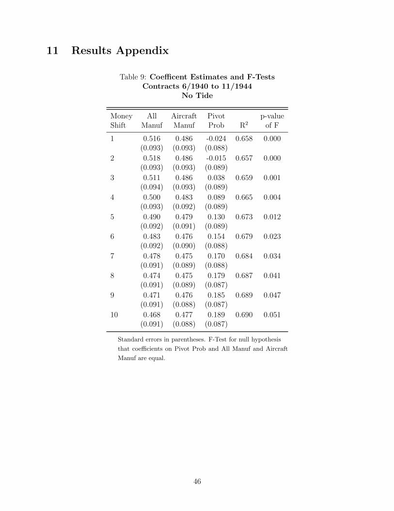
11 Results Appendix

Table 9: Coefficent Estimates and F-TestsContracts 6/1940 to 11/1944

No Tide

Money All Aircraft Pivot p-valueShift Manuf Manuf Prob R2 of F

1 0.516 0.486 -0.024 0.658 0.000(0.093) (0.093) (0.088)

2 0.518 0.486 -0.015 0.657 0.000(0.093) (0.093) (0.089)

3 0.511 0.486 0.038 0.659 0.001(0.094) (0.093) (0.089)

4 0.500 0.483 0.089 0.665 0.004(0.093) (0.092) (0.089)

5 0.490 0.479 0.130 0.673 0.012(0.092) (0.091) (0.089)

6 0.483 0.476 0.154 0.679 0.023(0.092) (0.090) (0.088)

7 0.478 0.475 0.170 0.684 0.034(0.091) (0.089) (0.088)

8 0.474 0.475 0.179 0.687 0.041(0.091) (0.089) (0.087)

9 0.471 0.476 0.185 0.689 0.047(0.091) (0.088) (0.087)

10 0.468 0.477 0.189 0.690 0.051(0.091) (0.088) (0.087)

Standard errors in parentheses. F-Test for null hypothesis

that coefficients on Pivot Prob and All Manuf and Aircraft

Manuf are equal.

46

The Arsenal of Democracy: Production and Politics During WWII

Documents