The Architecture of Growth: Product Space, Growth Acceleration, and "Small World" Networks

The Architecture of Growth: Product Space, Growth

Acceleration, and “Small World” Networks.

Raja Kali Josh McGee Javier Reyes

Stuart Shirrell1

Department of Economics

Sam M. Walton College of Business

University of Arkansas

Fayetteville, AR 72701

Incomplete. Please do not cite without permission.

October 2008

1Department of Economics, Sam M. Walton College of Business, University of Arkansas — U.S.A.;e-mail: [email protected], [email protected], [email protected], [email protected].

1 Introduction

What are the mechanics behind an acceleration in the economic growth rate for a country?

What role does trade and comparative advantage play in this process? These are among the

most enduring and important questions in economics.

On the first question, a recent paper by Hausman, Pritchett and Rodrik (2005) examines

“growth accelerations,” episodes of rapid acceleration in economic growth that are sustained

for at least eight years, and finds them to be highly unpredictable. The vast majority

of growth accelerations are unrelated to standard determinants such as political change and

economic reform, and most instances of economic reform do not produce growth accelerations.

This leaves us with a conundrum. Are growth accelerations idiosyncratic and/or a matter of

luck? The implications of such a conclusion would be distressing, to say the least. But while

the mechanics of these transitions continue to be a mystery, the good news is that Hausman

et al. find that growth accelerations are a fairly frequent occurrence. Of the 110 countries

in their sample, 60 have had at least one acceleration in the 35-year period between 1957 and

1992 — a ratio of 55 percent.

With regard to the second question, recent papers by Hausman and Bailey (2007) and

Hidalgo et. al. (2007) develop an innovative approach to the evolution of comparative

advantage that suggest a new way forward. Using detailed product-level data from the NBER

World Trade Database, these papers map the “product space,” of relatedness among products

based on the pattern of revealed comparative advantage in world trade. In other words, they

infer the network of relatedness among products from the observable export-mix in the data.

This indicates how likely it is for different products to be exported together. They then

ask if the pattern of product specialization of a country is densely or sparsely connected.

They identify two patterns here. First, the pattern of relatedness of products exhibits a high

degree of heterogeneity: there are parts of the product space that are dense while others are

sparse. More sophisticated products are located in a densely connected core whereas less

sophisticated products occupy a less-connected periphery. Second, changes in the revealed

comparative advantage of nations are governed by the pattern of relatedness at a global level.

Empirically, countries move through the product space by developing goods close to those

they currently produce. This implies that countries that are specialized in a dense part of

1

the product space have an easier time at changing their revealed comparative advantage than

countries that are specialized in more disconnected products. Most countries can reach the

core only by traversing empirically infrequent distances, which may help explain why poor

countries have trouble developing more competitive exports and fail to converge to the income

level of rich countries. The inability to make long-range leaps is associated with difficulty in

moving from low-growth (traditional/poor) products to high-growth (modern/rich) products.

Countries that have a comparative advantage in traditional products are likely to be stuck

in a “product-trap,” since they will only be able to produce products close to the ones they

already produce. According to this view, a country’s location in product space is a key

determinant of its growth capabilities.

Our insight builds upon these two strands of work to dispel some of the mystery behind

the mechanics of growth acceleration, and in doing so provides a unified relationship between

comparative advantage, trade, and economic growth. The work of Hausman and Bailey

(2007) and Hidalgo et. al. (2007) suggests a natural interpretation of “product space” in

terms of networks. We therefore adopt a network interpretation of product space and use

analytical methods from the recent literature on complex networks1. One of the general

results of this literature is that “successful” networks in many settings (biological, technolog-

ical, social, economic) have the “small world” property (Watts and Strogatz, 1998). In other

words, in many contexts, the small world seems to be an “optimal” topology. Small world

networks combine high clustering among nodes with high connectivity (short path length)

across nodes. High clustering suggests such networks are likely to have strong spillovers

between nodes, while short path length implies the possibility of long range leaps. Both fea-

tures are advantageous in the context of economic development and growth. Could it be that

the key to growth acceleration is whether the pattern of product specialization of a country

develops a “small world” topology before the take-off? If true, then this implies that it is

not just the country’s location in product space, but also (especially) the country’s pattern

of product specialization that matters. If we can find evidence for this line of reasoning,

then we will have made important progress in decoding the mystery of growth acceleration.

Our research project aims to marshall evidence to support this insight. We will do this in

1Newman (2000) and Albert and Barabasi (2002) are good overviews of this literature. The survey byJackson (2006) is a good introduction to the economics of networks.

2

several steps, the first of which is already complete. First, we chart the topology of product

space across time, from 1965 to 2000. This provides us with evidence that the product

space network of relatedness among products based on the pattern of revealed comparative

advantage in world trade has evolved considerably over time. We find that that the evolution

of product space experienced a structural break during the 1980’s. Second, we will map the

product specialization pattern of individual countries. Third, we will superimpose (country-

level) product specialization of countries that experienced episodes of growth acceleration on

the network of product space. Superimposing the country-level product specialization “sub”-

network on the larger product-space network will enable us to examine whether country-level

product specialization resembles a “small world” prior to the time of a growth acceleration.

Finally, we will run a multivariate regression to understand if there is large sample support

for the hypothesis that if a country’s pattern of product specialization resembles a small

world, then it is more likely to to experience subsequent growth acceleration.

The study of the relationship between trade and economic growth and development

has a long and distinguished pedigree in economics, going back to seminal explorations by

Rosenstein-Rodan (1943) and Hirschman (1958). The astounding performance of the east

Asian economies in the last quarter of the twentieth century reinvigorated this question, and

stimulated a number of recent contributions such as Grossman and Helpman (1991), Mat-

suyama (1992), Frankel and Romer (1999), and Rodriguez and Rodrik (2001), among others.

However, this question does not seem to be settled, either theoretically and empirically. We

believe that our research has the potential to bring a novel perspective to these issues.

In the next section we explain our hypothesis and the network approach in more detail.

We present a simple theoretical framework to ground our empirical analysis. Section 3

describes the evolution of the product space and country-level patterns of product special-

ization. We also summarize the conclusions from our empirical analysis thus far. Section 4

discusses broader implications of this research project.

2 Product Space, Country Specialization, and the SmallWorld

Product Space

We follow Hidalgo et. al. (2007) and Hausman and Bailey (2007) in computing the

3

product space of relatedness among products based on the pattern of revealed comparative

advantage in world trade. We provide a brief description here; the reader is referred to

their papers for more detail. Like them, we use the NBER World Trade Database for the

computation of product space (Feenstra et al., 2005).

The first step is the computation of “revealed comparative advantage” (RCA), which

measures whether a country c exports more of good i, as a share of its total exports, than

the “average” country (RCA > 1 not RCA<1).

RCAc,i =

x(c,i)

i x(c,i)

c x(c,i)

c,i x(c,i)

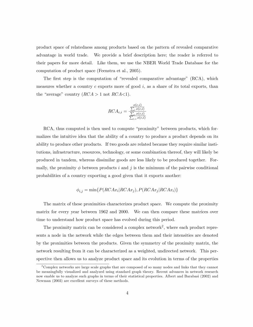
RCA, thus computed is then used to compute “proximity” between products, which for-

malizes the intuitive idea that the ability of a country to produce a product depends on its

ability to produce other products. If two goods are related because they require similar insti-

tutions, infrastructure, resources, technology, or some combination thereof, they will likely be

produced in tandem, whereas dissimilar goods are less likely to be produced together. For-

mally, the proximity φ between products i and j is the minimum of the pairwise conditional

probabilities of a country exporting a good given that it exports another:

φi,j = min{P (RCAxi|RCAxj), P (RCAxj |RCAxi)}

The matrix of these proximities characterizes product space. We compute the proximity

matrix for every year between 1962 and 2000. We can then compare these matrices over

time to understand how product space has evolved during this period.

The proximity matrix can be considered a complex network2, where each product repre-

sents a node in the network while the edges between them and their intensities are denoted

by the proximities between the products. Given the symmetry of the proximity matrix, the

network resulting from it can be characterized as a weighted, undirected network. This per-

spective then allows us to analyze product space and its evolution in terms of the properties

2Complex networks are large scale graphs that are composed of so many nodes and links that they cannotbe meaningfully visualized and analyzed using standard graph theory. Recent advances in network researchnow enable us to analyze such graphs in terms of their statistical properties. Albert and Barabasi (2002) andNewman (2003) are excellent surveys of these methods.

4

of the network.

Country Level Product Specialization

The set of products for which a country possesses RCA (>1) is what we refer to as country

level product specialization. This is essentially the comparative advantage of a country. We

can examine how this set has changed over the time period of our data for countries which

experienced growth acceleration and those that did not.

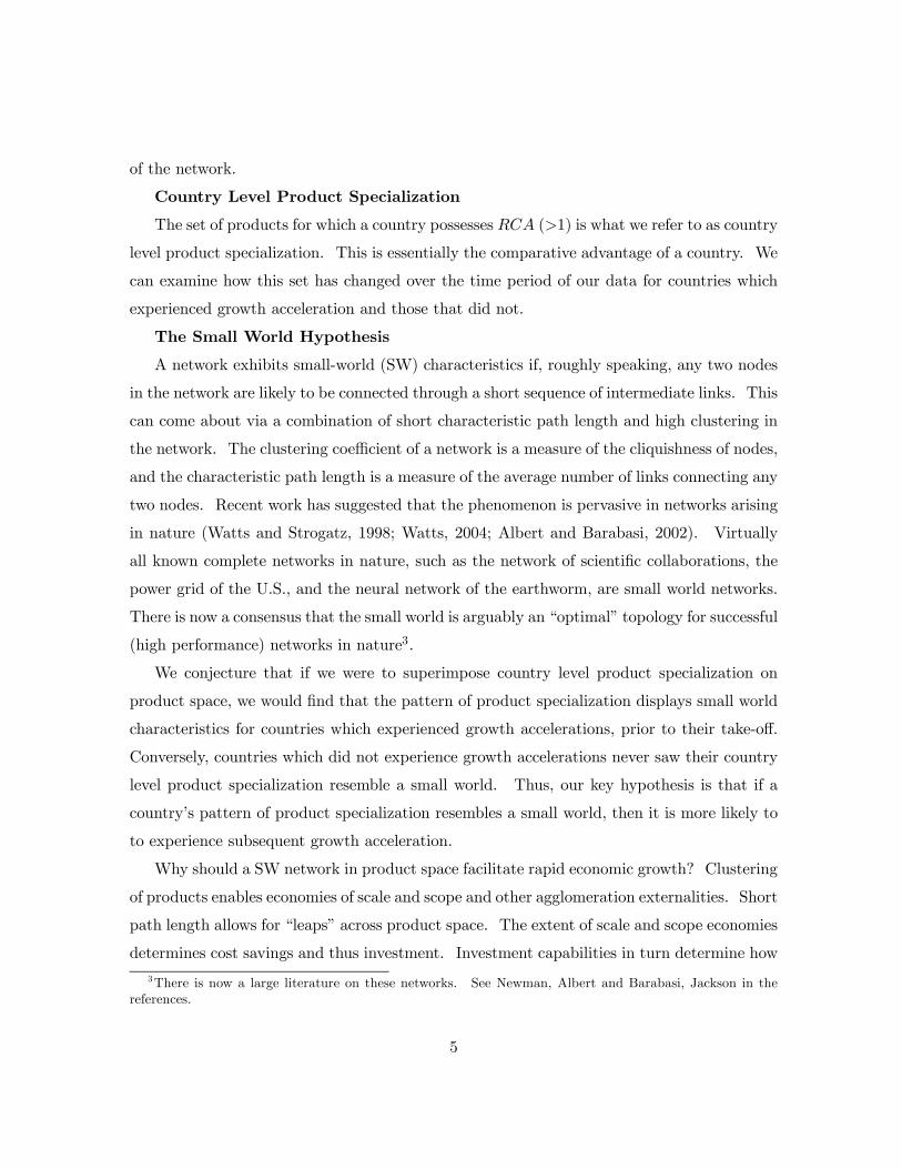
The Small World Hypothesis

A network exhibits small-world (SW) characteristics if, roughly speaking, any two nodes

in the network are likely to be connected through a short sequence of intermediate links. This

can come about via a combination of short characteristic path length and high clustering in

the network. The clustering coefficient of a network is a measure of the cliquishness of nodes,

and the characteristic path length is a measure of the average number of links connecting any

two nodes. Recent work has suggested that the phenomenon is pervasive in networks arising

in nature (Watts and Strogatz, 1998; Watts, 2004; Albert and Barabasi, 2002). Virtually

all known complete networks in nature, such as the network of scientific collaborations, the

power grid of the U.S., and the neural network of the earthworm, are small world networks.

There is now a consensus that the small world is arguably an “optimal” topology for successful

(high performance) networks in nature3.

We conjecture that if we were to superimpose country level product specialization on

product space, we would find that the pattern of product specialization displays small world

characteristics for countries which experienced growth accelerations, prior to their take-off.

Conversely, countries which did not experience growth accelerations never saw their country

level product specialization resemble a small world. Thus, our key hypothesis is that if a

country’s pattern of product specialization resembles a small world, then it is more likely to

to experience subsequent growth acceleration.

Why should a SW network in product space facilitate rapid economic growth? Clustering

of products enables economies of scale and scope and other agglomeration externalities. Short

path length allows for “leaps” across product space. The extent of scale and scope economies

determines cost savings and thus investment. Investment capabilities in turn determine how

3There is now a large literature on these networks. See Newman, Albert and Barabasi, Jackson in thereferences.

5

far a country can leap. Proximity in product space determines how far a country needs

to leap to the closest high-income product. The gap between these two plays a role in

determining growth acceleration. We present a simple formalization of this intuition below.

If product space is changing over time (due to changes in technology, preferences and

other effects), then a country with a particular pattern of product specialization might find

that the product space has moved to a configuration that creates advantageous conditions

for product leaps and thus faster growth. Product space evolves to intersect with a country’s

product specialization in such a way as to create a “small world” and enable product leaps.

Note that this is the converse of thinking that product space is fixed and it is country level

patterns of specialization evolve. Under this hypothesis, country-level patterns of specializa-

tion could remain relatively invariant, but what changes is product space. The key to growth

acceleration is thus essentially a matter of being “in the right space at the right time.”

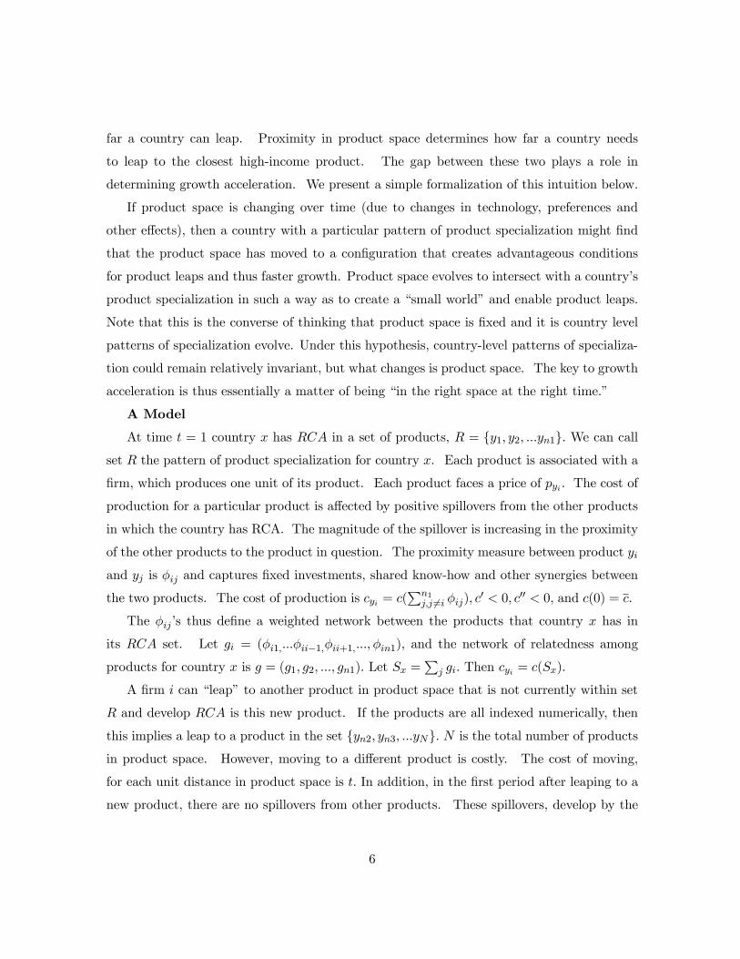
A Model

At time t = 1 country x has RCA in a set of products, R = {y1, y2, ...yn1}. We can callset R the pattern of product specialization for country x. Each product is associated with a

firm, which produces one unit of its product. Each product faces a price of pyi . The cost of

production for a particular product is affected by positive spillovers from the other products

in which the country has RCA. The magnitude of the spillover is increasing in the proximity

of the other products to the product in question. The proximity measure between product yi

and yj is φij and captures fixed investments, shared know-how and other synergies between

the two products. The cost of production is cyi = c(Pn1

j,j 6=i φij), c0 < 0, c00 < 0, and c(0) = c.

The φij ’s thus define a weighted network between the products that country x has in

its RCA set. Let gi = (φi1,...φii−1,φii+1,..., φin1), and the network of relatedness among

products for country x is g = (g1, g2, ..., gn1). Let Sx =P

j gi. Then cyi = c(Sx).

A firm i can “leap” to another product in product space that is not currently within set

R and develop RCA is this new product. If the products are all indexed numerically, then

this implies a leap to a product in the set {yn2, yn3, ...yN}. N is the total number of products

in product space. However, moving to a different product is costly. The cost of moving,

for each unit distance in product space is t. In addition, in the first period after leaping to a

new product, there are no spillovers from other products. These spillovers, develop by the

6

following period, and depend upon the density of the production cluster associated with the

new product.

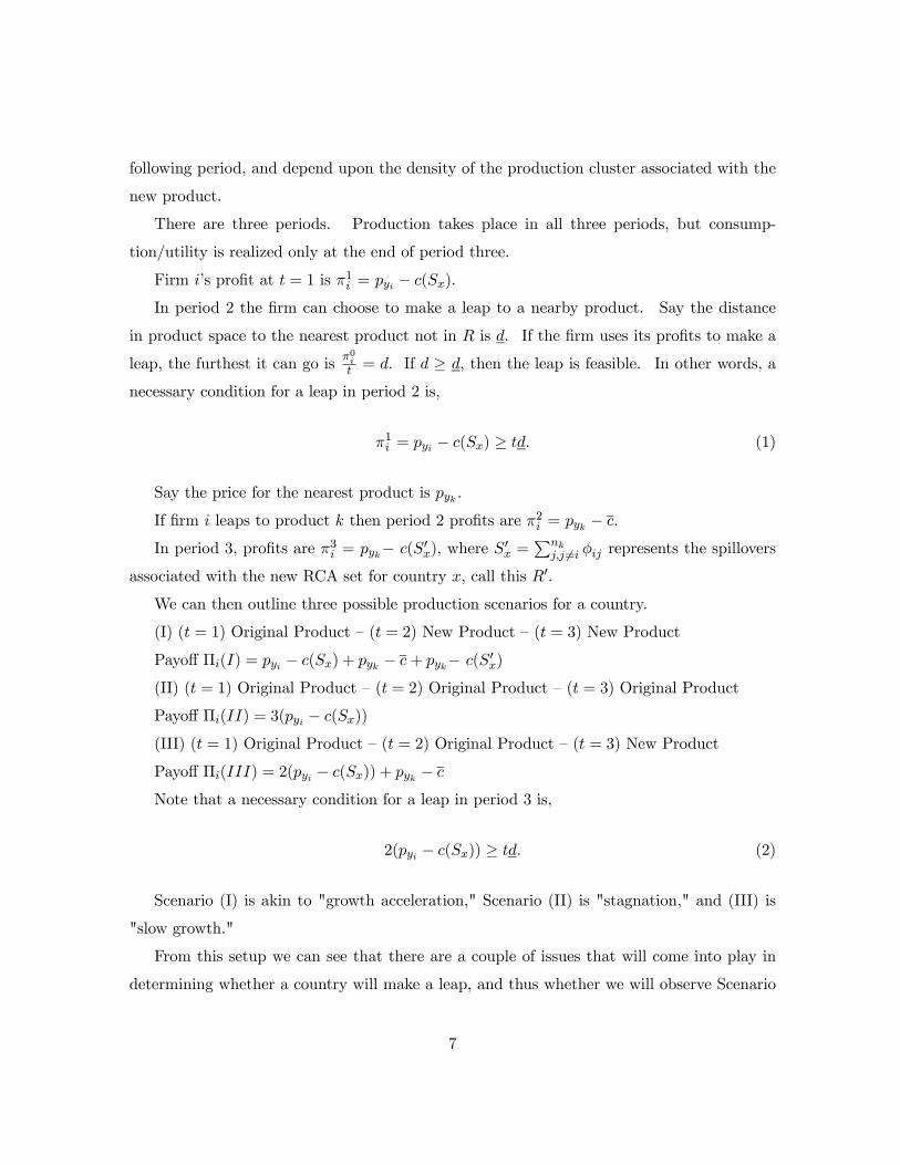
There are three periods. Production takes place in all three periods, but consump-

tion/utility is realized only at the end of period three.

Firm i’s profit at t = 1 is π1i = pyi − c(Sx).

In period 2 the firm can choose to make a leap to a nearby product. Say the distance

in product space to the nearest product not in R is d. If the firm uses its profits to make a

leap, the furthest it can go is π0it = d. If d ≥ d, then the leap is feasible. In other words, a

necessary condition for a leap in period 2 is,

π1i = pyi − c(Sx) ≥ td. (1)

Say the price for the nearest product is pyk .

If firm i leaps to product k then period 2 profits are π2i = pyk − c.

In period 3, profits are π3i = pyk− c(S0x), where S0x =

Pnkj,j 6=i φij represents the spillovers

associated with the new RCA set for country x, call this R0.

We can then outline three possible production scenarios for a country.

(I) (t = 1) Original Product — (t = 2) New Product — (t = 3) New Product

Payoff Πi(I) = pyi − c(Sx) + pyk − c+ pyk− c(S0x)

(II) (t = 1) Original Product — (t = 2) Original Product — (t = 3) Original Product

Payoff Πi(II) = 3(pyi − c(Sx))

(III) (t = 1) Original Product — (t = 2) Original Product — (t = 3) New Product

Payoff Πi(III) = 2(pyi − c(Sx)) + pyk − c

Note that a necessary condition for a leap in period 3 is,

2(pyi − c(Sx)) ≥ td. (2)

Scenario (I) is akin to "growth acceleration," Scenario (II) is "stagnation," and (III) is

"slow growth."

From this setup we can see that there are a couple of issues that will come into play in

determining whether a country will make a leap, and thus whether we will observe Scenario

7

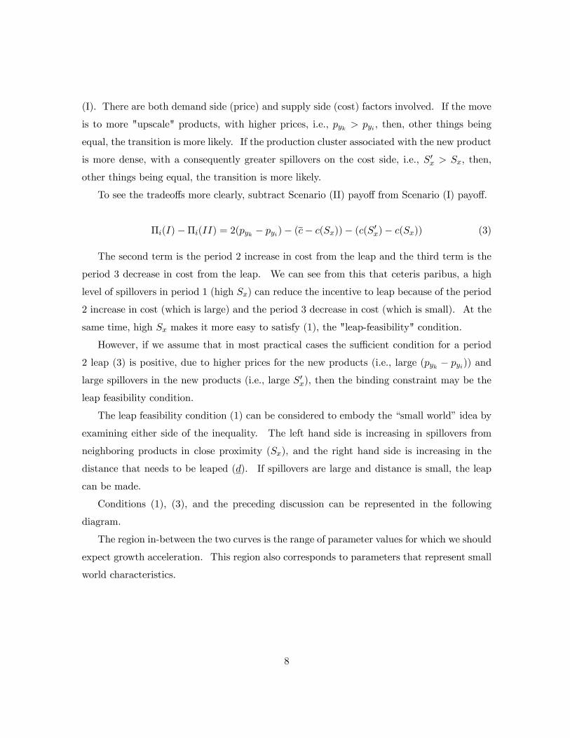
(I). There are both demand side (price) and supply side (cost) factors involved. If the move

is to more "upscale" products, with higher prices, i.e., pyk > pyi , then, other things being

equal, the transition is more likely. If the production cluster associated with the new product

is more dense, with a consequently greater spillovers on the cost side, i.e., S0x > Sx, then,

other things being equal, the transition is more likely.

To see the tradeoffs more clearly, subtract Scenario (II) payoff from Scenario (I) payoff.

Πi(I)−Πi(II) = 2(pyk − pyi)− (c− c(Sx))− (c(S0x)− c(Sx)) (3)

The second term is the period 2 increase in cost from the leap and the third term is the

period 3 decrease in cost from the leap. We can see from this that ceteris paribus, a high

level of spillovers in period 1 (high Sx) can reduce the incentive to leap because of the period

2 increase in cost (which is large) and the period 3 decrease in cost (which is small). At the

same time, high Sx makes it more easy to satisfy (1), the "leap-feasibility" condition.

However, if we assume that in most practical cases the sufficient condition for a period

2 leap (3) is positive, due to higher prices for the new products (i.e., large (pyk − pyi)) and

large spillovers in the new products (i.e., large S0x), then the binding constraint may be the

leap feasibility condition.

The leap feasibility condition (1) can be considered to embody the “small world” idea by

examining either side of the inequality. The left hand side is increasing in spillovers from

neighboring products in close proximity (Sx), and the right hand side is increasing in the

distance that needs to be leaped (d). If spillovers are large and distance is small, the leap

can be made.

Conditions (1), (3), and the preceding discussion can be represented in the following

diagram.

The region in-between the two curves is the range of parameter values for which we should

expect growth acceleration. This region also corresponds to parameters that represent small

world characteristics.

8

Sx

d, Pyk‐Pyj

No Transition

Transition

Product Leap FeasibilityConstraint

Product Leap IncentiveConstraint

No Incentive

Incentive

Figure 1: Product Leaps

9

3 The Evolution of the Product Space

The first step in our methodology is to describe the evolution of the product space of related-

ness among products between 1962 and 2000. The product space is defined by the proximity

matrix introduced in the previous section and can be considered a complex network where

each product represents a node in the network while the edges between them (and their in-

tensities) are denoted by the proximities between the products. Given the symmetry of the

proximity matrix, the network resulting from it can be characterized as a weighted and undi-

rected network. With this framework, we attempt to analyze the evolution of the properties

of the product space by using a variety of network indicators. This section presents a series

of network analyses that show that the product space has changed over the past 30 years.

The set of communities, the density of the product space, the distribution of proximities, and

the clustering between industries is studied in detail.

3.1 Correlation between Product Space Proximities across Time

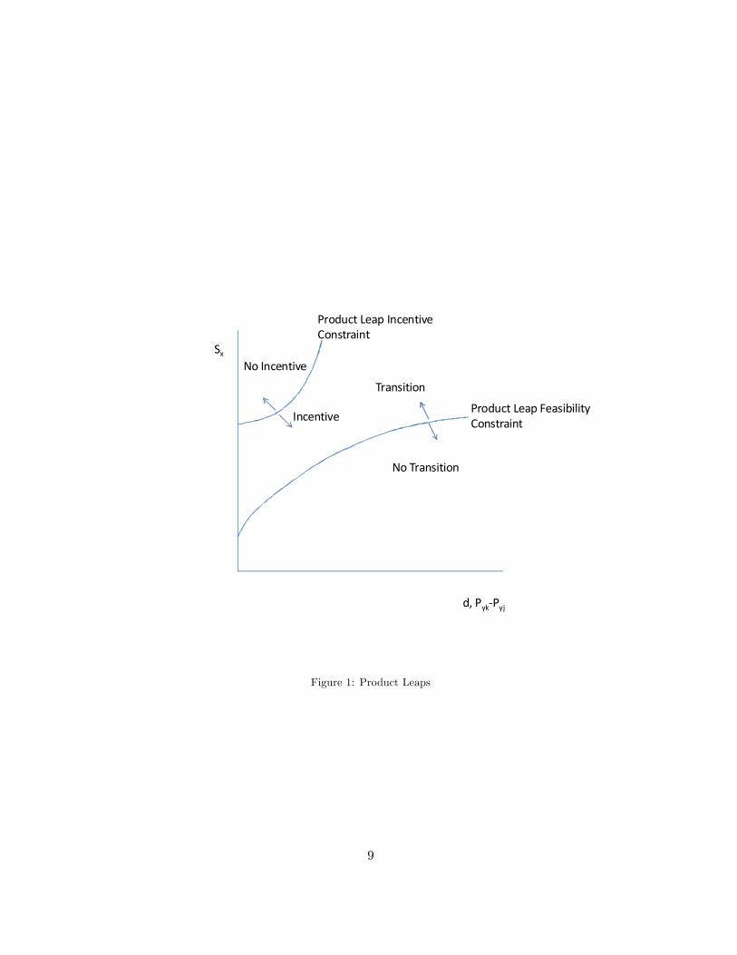
The simplest way for the analysis of the changes in the product space is to compute the

Pearson correlation coefficient for the proximities between each pair of products across time.

The correlation coefficients across time fall dramatically once the correlation is computed

1962 1965 1970 1975 1980 1985 1990 1995 20001962 11965 0.93 11970 0.90 0.97 11975 0.69 0.76 0.81 11980 0.62 0.68 0.73 0.91 11985 0.36 0.42 0.46 0.58 0.72 11990 0.29 0.34 0.38 0.50 0.62 0.94 11995 0.16 0.20 0.24 0.35 0.43 0.69 0.83 12000 0.16 0.20 0.24 0.35 0.43 0.68 0.81 0.98 1

Table 1: Pearson Correlation Coefficient for Proximities between Product Pairs

between product spaces more than ten years apart, and there is no correlation above 0.79.

In addition, it is noteworthy that there is a sharp fall in the correlation coefficient in the early

eighties. The correlation for a year on year comparison is always above 0.80 for all years,

except when 1980 is compared to 1975.

10

3.2 Network Density and the Distribution of Weighted Links

Next we look at two simple indicators which provide insight into how product space has

changed over time. The first is network density, the number of links present in the network

as a percentage of the maximum possible. The second is the distribution of the weighted

links. Examining network density and the distribution of weighted links together allows us to

understand whether the changes have been quantitative instead of qualitative. For instance,

it could be that the number of products that are likely to be exported together has increased

but the likelihoods are very small. In other words more of the proximities between products

are now different from zero, but they are just marginally positive. A different scenario would

be the case in which the number of products that are likely to be exported together remains

constant, but the likelihood (proximity) becomes much greater.

The results presented in Figures 2 and 3 show evidence for relatively signficant changes

of the product space. Regarding density (i.e., number of products exported together), we

see it clearly accelerated in between 1975 and 1980 where it increased from 0.45 to 0.88 and

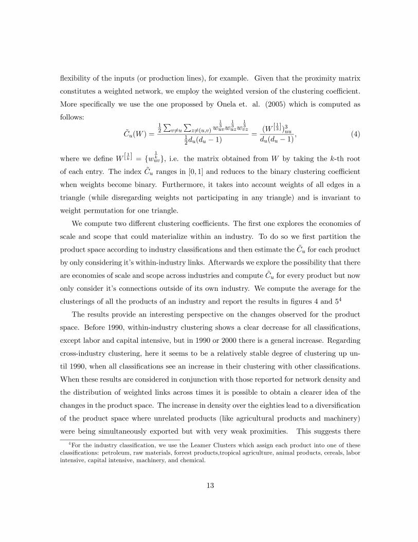
then came back down to 0.65 in the mid nineties. Regarding the distribution of the weighted

links, the changes are less visible but, nonetheless, still present. Figure 3, which presents

the kernel density distributions for the years 1975, 1985, and 2000, shows that there has

been a an amplification in the magnitude of the proximities between the products present

in the product space. Interestingly, the increase in density observed in the eighties (Figure

2) coincides with an increase in the number of high weighted links in the product space.

Evidence of this is the rightward shift of the probability mass observed for 1985 in Figure 3.

Additionally, the drop in density during the nineties actually corresponded to a drop of low

weight links in the product space.

3.3 Clustering in Product Space

The clustering coefficient of a given node is defined as the ratio of the number of triangles

with node i as one vertex to the total number of triangles that node i could have been a

part of (which is determined by its degree). Within the product space context, clustering can

shed some light on economies of scale and scope leading to the simultaneous export of certain

products. These economies could result from the similarities of the product or due to the

11

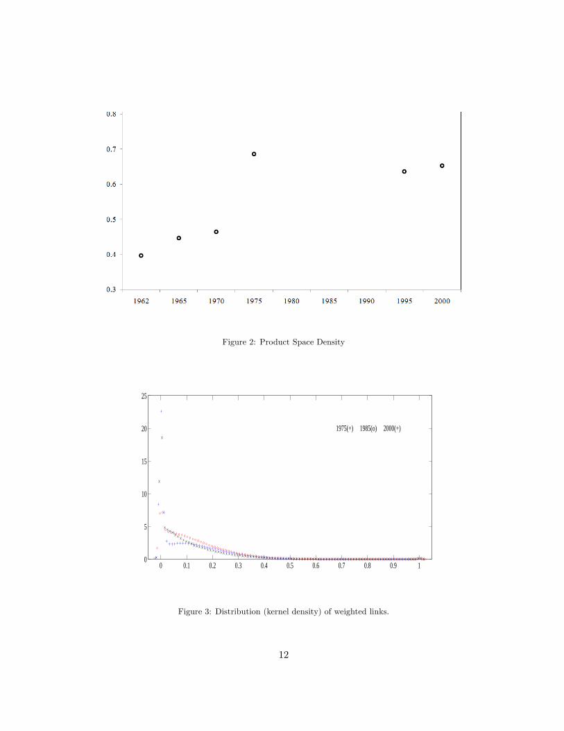
Figure 2: Product Space Density

0 0.1 0.2 0.3 0.4 0.5 0.6 0.7 0.8 0.9 10

5

10

15

20

25

1975(+) 1985(o) 2000(+)

Figure 3: Distribution (kernel density) of weighted links.

12

flexibility of the inputs (or production lines), for example. Given that the proximity matrix

constitutes a weighted network, we employ the weighted version of the clustering coefficient.

More specifically we use the one propossed by Onela et. al. (2005) which is computed as

follows:

C̃u(W ) =

12

Pv 6=u

Pz 6=(u,v)w

13uvw

13uzw

13vz

12du(du − 1)

=(W [ 13 ])3uudu(du − 1)

, (4)

where we define W [ 1k ] = {w1kuv}, i.e. the matrix obtained from W by taking the k-th root

of each entry. The index C̃u ranges in [0, 1] and reduces to the binary clustering coefficient

when weights become binary. Furthermore, it takes into account weights of all edges in a

triangle (while disregarding weights not participating in any triangle) and is invariant to

weight permutation for one triangle.

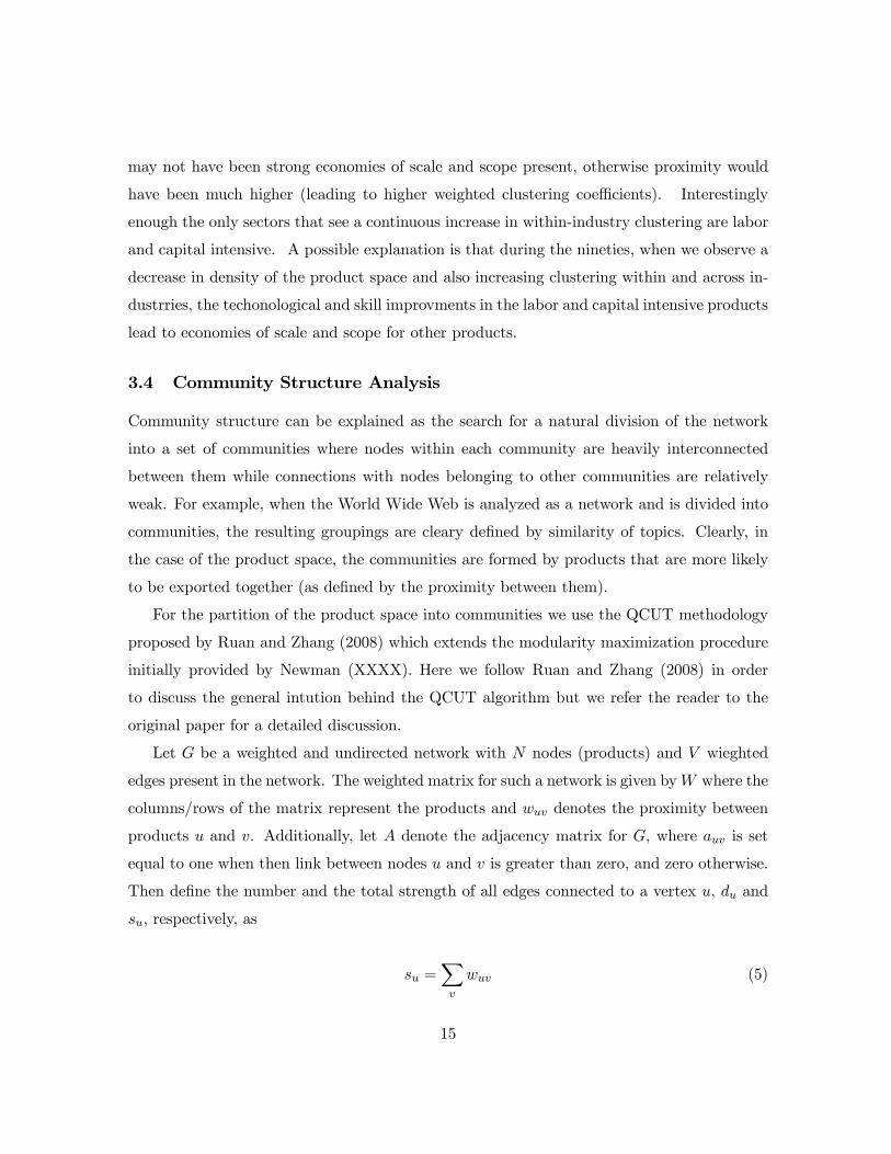
We compute two different clustering coefficients. The first one explores the economies of

scale and scope that could materialize within an industry. To do so we first partition the

product space according to industry classifications and then estimate the C̃u for each product

by only considering it’s within-industry links. Afterwards we explore the possibility that there

are economies of scale and scope across industries and compute C̃u for every product but now

only consider it’s connections outside of its own industry. We compute the average for the

clusterings of all the products of an industry and report the results in figures 4 and 54

The results provide an interesting perspective on the changes observed for the product

space. Before 1990, within-industry clustering shows a clear decrease for all classifications,

except labor and capital intensive, but in 1990 or 2000 there is a general increase. Regarding

cross-industry clustering, here it seems to be a relatively stable degree of clustering up un-

til 1990, when all classifications see an increase in their clustering with other classifications.

When these results are considered in conjunction with those reported for network density and

the distribution of weighted links across times it is possible to obtain a clearer idea of the

changes in the product space. The increase in density over the eighties lead to a diversification

of the product space where unrelated products (like agricultural products and machinery)

were being simultaneously exported but with very weak proximities. This suggests there

4For the industry classification, we use the Leamer Clusters which assign each product into one of theseclassifications: petroleum, raw materials, forrest products,tropical agriculture, animal products, cereals, laborintensive, capital intensive, machinery, and chemical.

13

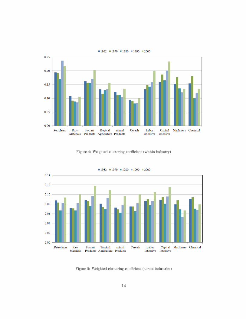
Figure 4: Weighted clustering coefficient (within industry)

Figure 5: Weighted clustering coefficient (across industries)

14

may not have been strong economies of scale and scope present, otherwise proximity would

have been much higher (leading to higher weighted clustering coefficients). Interestingly

enough the only sectors that see a continuous increase in within-industry clustering are labor

and capital intensive. A possible explanation is that during the nineties, when we observe a

decrease in density of the product space and also increasing clustering within and across in-

dustrries, the techonological and skill improvments in the labor and capital intensive products

lead to economies of scale and scope for other products.

3.4 Community Structure Analysis

Community structure can be explained as the search for a natural division of the network

into a set of communities where nodes within each community are heavily interconnected

between them while connections with nodes belonging to other communities are relatively

weak. For example, when the World Wide Web is analyzed as a network and is divided into

communities, the resulting groupings are cleary defined by similarity of topics. Clearly, in

the case of the product space, the communities are formed by products that are more likely

to be exported together (as defined by the proximity between them).

For the partition of the product space into communities we use the QCUT methodology

proposed by Ruan and Zhang (2008) which extends the modularity maximization procedure

initially provided by Newman (XXXX). Here we follow Ruan and Zhang (2008) in order

to discuss the general intution behind the QCUT algorithm but we refer the reader to the

original paper for a detailed discussion.

Let G be a weighted and undirected network with N nodes (products) and V wieghted

edges present in the network. The weighted matrix for such a network is given byW where the

columns/rows of the matrix represent the products and wuv denotes the proximity between

products u and v. Additionally, let A denote the adjacency matrix for G, where auv is set

equal to one when then link between nodes u and v is greater than zero, and zero otherwise.

Then define the number and the total strength of all edges connected to a vertex u, du and

su, respectively, as

su =Xv

wuv (5)

15

and

du =Xv

auv. (6)

Assuming that the nodes/products in G have been partitioned into k mutually exclusive

communities, c1, c2, ...,ck, then define eij as the sum of the magnitude of all edges connecting

vertices in community i and community j, represented as follows

eij =X

u∈ci,v∈cjwuv. (7)

Notice that eii would represent twice the total value of the edges with both ends within

community i. Let also ai be the total strength for the nodes included in community i,

ai =Xu∈ci

su. (8)

Then following Newman and Girvan (2004), the modularity of G for a particular partition

of the network is defined by

Q =kXi=1

heiiM−³ aiM

´2i(9)

where M represents twice the total value of all edges present in the network. The first

term in equation 9 measures the fraction of total strength of edges present inside community

i, while the second term denotes the expected value for such fraction if the weighted edges

within the network were rewired, keeping du fixed for every u. Therefore, the objective of the

community structure algorithms that use the modularity approach is to maximize the value

of Q. This is because higher values of Q denote higher intracommunity connectivity (by

number and value of the edges). 5. The problem with the maximization of the modularity is

that it has been shown that an efficient optimal algorithm is unlikely to exist.

Ruan and Zhang (2008) proposed a heuristic algorithm referred to as QCUT that provides

a good approximation for the maximization of Q. The specifics of their methodology are not

discussed here for matters of scope and space, but intuitively this algorithm is based on two

5It is clear that when the network is comprised of one community then Q = 0, also the expected valuefor randomly partitioning a network is also equal to zero. But a random network can have positive or evensubstantial modularity, especially for sparse networks

16

steps.6 First, it uses a spectral graph algorithm to recursively divide the network until

no improvements to Q, equation (9), can be achieved. Therefore, it provides an efficient

approximation to find a relatively good Q. Afterwards, a routine where nodes are moved to

different communities or communities are merged in an attempt to improve Q is applied, this

is referred to as the refinement stage. These two steps, partition and refinement, are done

recursively until neither improves Q.

The objective of using the QCUT algorithm is to provide some basis of comparison for

the product space across time. Once the proximity matrices for two different years have

been partitioned into their optimal communities, it is then possible to see how well their

communities match. Visually one can use the community partition of one year and use it to

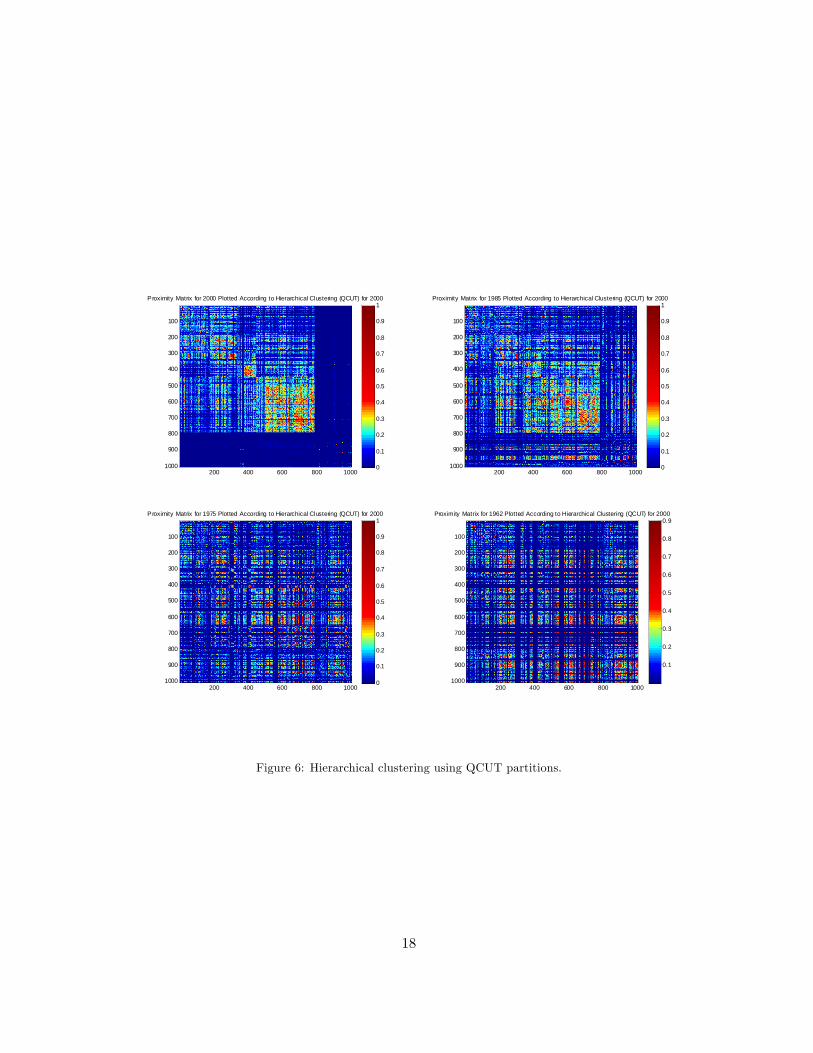
sort the product space of that year into clusters. In Figure 6, which shows the hierarchical

clustering for the proximity matrix in 2000 using the community partition for this year, it

is easy to identify the highly clustered regions in the product space. In order to show the

changes in the product space, Figure 6 also shows the results for the product spaces of 1975,

1985, and 1995 when these are partitioned according to the community structure of the

product space of 2000. We can see that the highly clustered regions of the 2000 product

space are not the same as those of 1975. Moreover, there even are some sllight differences

between the 1995 and the 2000 data.

Although the visual representation of the changes of the product space through time

seems very convincing, we also use more rigorous tools for this comparison. This is another

advantage of using the community structure for the analysis of the product space. Given a

two community partition, a benchmark and an alternative, it is possible to asses the number

of intracommunity vertex pairs that are identified in both partitions. Here we use three

different indices for this comparison, the Jaccard Index, the Fowlkes and Mallows Index,

and the Variation of Information approach. Intuitively, assume a benchmark community

structure C1 and an alternative one referred to as C2, then let S1 be the set of vertex pairs

in the same community in C1, and S2 the set of vertex pairs in the same community in C2.

6The interested reader is referred to the original article for more details

17

Proximity Matrix for 2000 Plotted According to Hierarchical Clustering (QCUT) for 2000

200 400 600 800 1000

100

200

300

400

500

600

700

800

900

1000 0

0.1

0.2

0.3

0.4

0.5

0.6

0.7

0.8

0.9

1Proximity Matrix for 1985 Plotted According to Hierarchical Clustering (QCUT) for 2000

200 400 600 800 1000

100

200

300

400

500

600

700

800

900

1000 0

0.1

0.2

0.3

0.4

0.5

0.6

0.7

0.8

0.9

1

Proximity Matrix for 1975 Plotted According to Hierarchical Clustering (QCUT) for 2000

200 400 600 800 1000

100

200

300

400

500

600

700

800

900

1000 0

0.1

0.2

0.3

0.4

0.5

0.6

0.7

0.8

0.9

1Proximity Matrix for 1962 Plotted According to Hierarchical Clustering (QCUT) for 2000

200 400 600 800 1000

100

200

300

400

500

600

700

800

900

1000

0.1

0.2

0.3

0.4

0.5

0.6

0.7

0.8

0.9

Figure 6: Hierarchical clustering using QCUT partitions.

18

Then the Jaccard Index, which lies between 0 and 1, can be computed as

J(S1, S2) =|S1TS2|

|S1SS2|

(10)

In the case of the Fowlkes and Mallows Index, what is measured is the probability of a pair

of vertices which are in the same community under C1 are also in the same community under

C2, and the index is between 0 and 1. With respect to the Variation of Information index,

this one measures the ammount of information lost or gained in changing from C1 to C2,

it is always non-negative, and zero denotes the best accuracy. The specifics of the Fowlkes

and Mallows Index and the Variation of Information Index are discussed in detail in Tan,

Steinback, and Kumar(2005), Fowlkes and Mallows (1983), and Meila (2007), respectively.

For the benchmark community this study uses the one resulting for the product space

of 2000 and then compares the community structures of all the other years against this

benchmark. The results, presented in Figure 7, support the argument of a changing product

space through time. One aspect that is gained by moving from the visual results of Figure

7 is that a clear break point is identified. There is a change in the slope of the degree of

difference, as measured by the indices discussed above, between the product space of 2000

and the previous years. This change in the slope takes place in 1980. This suggests that the

product space suffered accelerated changes during the 1980 to 2000 period but this change

was much slower before 1980. Even between 2000 and 1995 the correspondence of vertex

pairs between partitions is only between seventy to eighty percent.

3.5 Summary

The evolution in the product space network between 1962 and 2000 based on the measures

computed above can be summarized as follows:

1. The qualitative nature of the network of relatedness between products changed consid-

erably from 1962 to 2000. The network, as described by the correlation of proximity

over time is substantially different in 2000 as compared to 1965. This is also evident

from the change in hierarchical community structure in the network. The community

structure in the network of relatedness between products in 2000 is a poor description

19

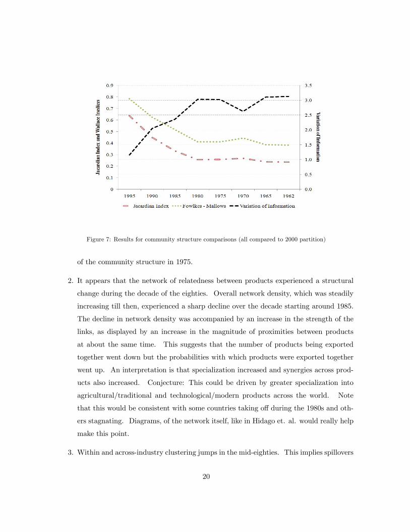
Figure 7: Results for community structure comparisons (all compared to 2000 partition)

of the community structure in 1975.

2. It appears that the network of relatedness between products experienced a structural

change during the decade of the eighties. Overall network density, which was steadily

increasing till then, experienced a sharp decline over the decade starting around 1985.

The decline in network density was accompanied by an increase in the strength of the

links, as displayed by an increase in the magnitude of proximities between products

at about the same time. This suggests that the number of products being exported

together went down but the probabilities with which products were exported together

went up. An interpretation is that specialization increased and synergies across prod-

ucts also increased. Conjecture: This could be driven by greater specialization into

agricultural/traditional and technological/modern products across the world. Note

that this would be consistent with some countries taking off during the 1980s and oth-

ers stagnating. Diagrams, of the network itself, like in Hidago et. al. would really help

make this point.

3. Within and across-industry clustering jumps in the mid-eighties. This implies spillovers

20

are likely to have gone up starting in the mid-eighties. This is actually a conjecture,

since the clustering figures at the moment show a decline in 1980 and sudden increase

in 1990. Our conjecture is that the jump might actually be in the mid-eighties.

4. The next step involves superimposing country-level patterns of product specialization

on product space to examine for the “small-world” hypothesis.

4 Broader Implications: The Architecture of Growth

We believe that a network approach along the lines described has the potential to uncover

“structural” properties of product specialization, comparative advantage and their relation-

ship to economic growth that have not been examined in the literature. If we find support

for the hypothesis that there is a unifying pattern in the way in which the products that a

country posseses comparative advantage are related (such as a small world topology), then we

will have made important progress in decoding the mystery of growth acceleration. This in

turn will lead to important implications for industrial and development policy. For example,

it could suggest ways in which a country could target or prioritize sectors of the economy

given its current pattern of product specialization so as to be well-primed for a development

trajectory.

The network-based methodology can unravel characteristics of the growth acceleration

process that are difficult to both see and understand using conventional approaches. In this

sense, the methodology itself can expand the scope of the questions that we will be able to

ask. For example, the literature on complex networks proposes many ways in which the small

world configuration (SW) may arise (short-cuts, hubs, modularity). This in turn suggests

that a number of different policies/accidents could lead to this optimal configuration. A

diversity of ways may lead to the possibility of growth acceleration. In this spirit, a logical

next step in this research agenda would be to examine the diversity of ways in which the

product specialization network of countries that experienced episodes of growth acceleration

approximates the optimal topology.

21

References

[16] Albert, A. and A. L. Barabasi, (2002), “Statistical Mechanics of Complex Networks”,

Reviews of Modern Physics 74, 47.

[16] Barabasi, A. (2002), Linked: The New Science of Networks, Perseus Publishing, Cam-

bridge, MA.

[16] Frankel, Jeffrey A. and David Romer (1999), “Does Trade Cause Growth?” American

Economic Review, vol. 89, no. 3, pp. 379-399.

[16] Goyal, S., M. J. van der Leij (2006), “Economics: An Emerging Small World,” Journal

of Political Economy, 11(2): 403-412.

[16] Grossman, G. and E. Helpman (1991), Innovation and Growth in the Global Economy,

MIT Press, Cambridge, MA.

[16] Hausmann, Ricardo, Lant Prichett, and Dani Rodrick (2005), "Growth Accelerations,"

Journal of Economic Growth, 10(4): 303-329.

[16] Hausman, R. and B. Klinger (2007), “The Structure of the Product Space and the Evolu-

tion of Comparative Advantage,” Working Paper, Kennedy School, Harvard University.

[16] Hidalgo, C.A., Klinger, B., Barabasi, A.L. and R. Hausman (2007), “"The Product

Space Conditions the Development of Nations,” Science, 27 July 2007, Vol 317: 482-487.

[16] Hirschman, A. (1958), The Strategy of Economic Development, New Haven, Conn.:

Yale University Press.

[16] Feenstra, R. C., R.E. Lipsey, Deng, H., Ma, A.C. and Hengyong Mo, (2005),“World

Trade Flows, 1962-2000,” NBER Working Paper 11040.

[16] Jackson, M. O. (2006), “The Economics of Social Networks,” in Advances in Economics

and Econometrics, Theory and Applications: Ninth World Congress of the Econometric

22

Society, edited by Richard Blundell, Whitney Newey, and Torsten Persson, Chapter 1,

Volume I, Cambridge University Press.

[16] Matsuyama, Kiminori (1992), “Agricultural Productivity, Comparative Advantage, and

Economic Growth”, Journal of Economic Theory, vol. 58, no. 2, pp. 317-334.

[16] Rodriguez, Francisco and Dani Rodrik (2001), “Trade Policy and Economic Growth: A

Sceptic’s Guide to the Cross-National Evidence”, NBER Macroeconomics Annual 2000.

Cambridge, MA: MIT Press, pp. 261-324.

[16] Newman, M. E. J. (2003), “The Structure and Function of Complex Networks”, SIAM

Review 45, 167-256.

[16] Watts, D. J. and S. H. Strogatz. (1998) “Collective Dynamics of ‘Small-World’ Net-

works”, Nature 393:440-442.

[16] Watts, D. (2003), Six Degrees: The Science of a Connected Age, W.W. Norton, New

York & London.

23