The Applicationof State Variable Feedback Control todigital.lib.kmutt.ac.th/journal/kmuttv20n2_1.pdf2 The Applicationof State Variable Feedback Control to Fermentation Process Pipat

1

2

The Application of State Variable Feedback Control to

Fermentation Process

Pipat Titapand ’ and Ake Chaisawadi 2

King Mongkut’s Institute of Technology Thonburi

Abstract

The PID control technique uses open loop transfer function analysis and feedback

compensator design. By using this technique, it is difficult to control non-linear and time varying

systems, then a closed loop pole placement technique has been introduced in modern control

process and it is widely used in the state variable feedback control.

The application of state variable feedback control to the fermentation process is pro-

posed in this paper. A microprocessor based state variable feedback controller has been designed

and constructed for controlling a baker yeast fermentation process system fed by molasses. The

controller receives state variables from a sensor and the variables are provided in matrix form.

This paper also includes state observer method for calculate the gain of the controller.

The experimental results show that this controller can control multivariable at the same

time, ensure the accuracy of set point value, and transmit data to computer for analysis by serial

port of controller. This design emphasizes on easy data entering. The results can be shown by

LCD display or printer. This method also increases quality control for the process.

Graduate Student, Department of Electrical Engineering

Associate Professor, Department of Control System and Instrumentation Engineering

1. w-ii1

4

X=AX+BU (3.1)

U=-GX (3.2)

i=[~-BG]X (3.3.a)

X(s) = [SI - A + BG]-’ X(0) (3.3.b)

det[SI- A + BG] = Sk i-&S’-’ -&Sk-* +...+&_$+& =o

x = TX2 = TAT-’

(3.6.a)

(3.6.b)

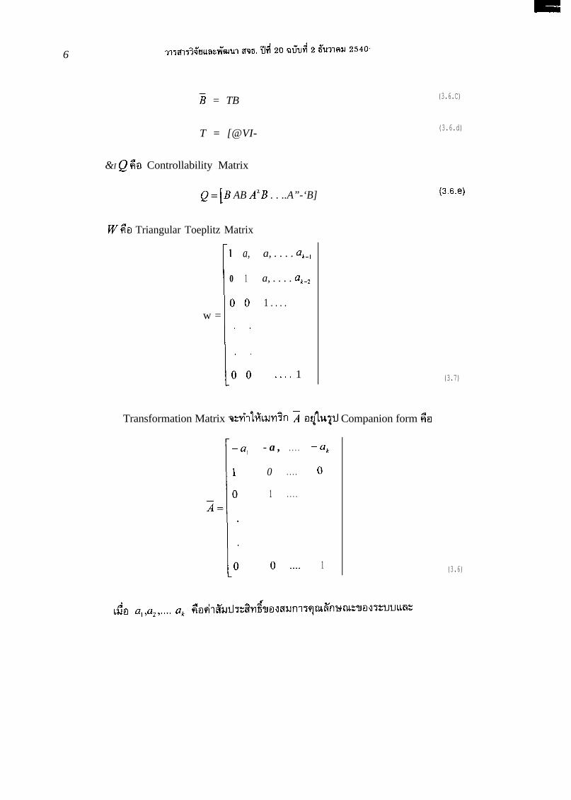
6

B = TB

T = [@VI-

&I Q zo Controllability Matrix

Q=[B AB A’B . . ..A”-‘B]

w so Triangular Toeplitz Matrix

1 1 a, a, . . . . a,_,

0 1 a, . . . . ak_*

0 0 1 . . . .w =

I. .. .

0 0 . . . . 1

Transformation Matrix ?.z'h%fiM~%l 2 a$.¶~@ Companion form zo

- a , . . . .

0 . . . .

1 . . . .

- ‘k

0

1

(3.6.C)

(3.6.d)

(3.6.e)

(3.7)

(3.6)

7

(3.9)

1 g,, s,, ..... s,0 0 0 . . . . . 0

- -B G = .

s,, &.. . .

Sk 1 = . , .. .0 0 0 . . . . .

--A-BG=

-a, -s, - a2 -S, . . . ..-ak -i,1

1 0 . . . . . 0

0 1 . . . . .

0 0

(3.10)

8

9, = a, -a,

-_u = -GX = #I(;) z-G x

(3.12.a)

(xmb)

Gt =Tt ct = T’(k) (3.12.C)

G ’ =[(QFV)‘j-’ (&) (3.12.d)

2,..... =.

-22 _

7r -

442 z. . . . . . . . . . . . +A+&_ _-t _

4. . . . . . u+ :.. [y-c,i,]B.2_ -4 _ (3.13)

(3.14)

(3.15)i = FZ+Gy+HU

e1

H

e = . . . =

e2

X, 2,. . . . . . . . . . . . .x,-i2:

9

(3.16)

.e2 = Fe, + (A,, - LC,A&C, + FLC,)X, +(A22 - LC,A,, - F)X2

+(B2 - LC,B, - H)U (3.17.a)

5 = [A,, - LC,A,, + FL+-’

H = B2 - LC,B,

F = A22 - LC,A,,

(3.17.b)

(3.17.c)

(3.17.d)

dm.m73 (3.17.a) -wwiierLh

e2 = Fe, (3.18)

xr-m~aJnl5 (2.18) w¶~hil eigen uosLuw%l F +um@J~~ua~Luw'ifl L &¶~~L~~n

L LI&U-?IHU~~~ eigen YEN Lam% F ki n"i rank WIN Observability Matrix N, LY%J k-l

do N, = (A,2)T,CT A22T A,,CT . . . . . (A22T)k - l

A,2TC,T 1 (3.19)

i = Fiz+(A,, - LC,A,,)C,-‘y+ HU (3.20.a)

_k, = Ly+Z (3.20.b)

10

i = [A-BG]X

i- = LY+Z

i = FZ+GY+HU

det[SI - A + BG] = det[SI - F] = 0

(3.21)

(3.22)

(3.23)

(3.24)

11

AIDConverter=ECPU

D/AConverter

c)start

1 input 1 ;r, \ --I 1 1TmntatlonProcess

I

\ ‘-‘----II- \

-Yes-Analysis9

No

Clock Pulse

ILimit raise

pulse

ILimit Lower

pulse

Set Point +-

Error Signal

I I

Calculate Controlledx(k+l)=Ax(k)+BU(k) Gain Matrix Variable

), U(k)= -Gx(k)Equation : X1-3.4

-+ (G)Equation: I

1 353.12 1 +

_

36 ~_................._. ......................... .................................................. ........ ..... .._......._......._. ............................................................................................................... ................................. i/

31 /

26

21

16

7

6.5

6

5.5

5

4.5

15

IS

I7

I9

21

2 23

”5 25

27

29

I5

I7

19

21

=! 23I3 253

27

29

31

33

35

37

39

41

43

45

47

I ILlB zJ6 ns”

7 .-

9 --

II .-

I3 _-

I5 .-

I7 .-

I9 .-

21 .-

; 23 .-

2.5 25-- --

27 --

29 .-

31 _-

33 ._

35 .-

37 ._

39 --

41 --

43 --

45 .-

47 .-

I IcljP3”

17

18

1 3 5 7 9 11 13 15 17 19 21 23 25 27 29 31 33 35 37 39 4 1 L - - - i~ State

Time (Hours)

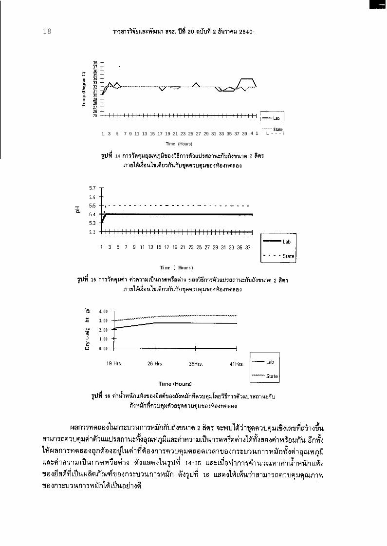
?tid 14 ni~~~qu?nms?u’YoJ~~nl~~~u~~~nlu~~~~~~ul~ 2 %I,

5.7

5.6

5.2

Time ( Hours)

Ii%I 4.00-E 3.00.g 2.003 1.00$ 0.00

REFERENCES .

1. Auslunder, D.M., Takahashi, Y., and Mizuka, M., 1980, “Direct Digital Process Control:Practical and Algorithms for Microprocessor Application.” Pvoc. IEEE., Vol. 6. No.2,pp.199-208.

2.

3.

Chiu, KC.. Corripio, A.B., and Smith, C.L.. 1973, “Digital Control Algorithms Part I:Dahlin Algorithms.” Instrument and Control System, Vol.10, pp. 57-59.

Chiu, K.C., Corripio, A.B., and Smith, C.L.. 1973. “Digital Control Algorithms Part II:Kalman Algorithms.” Instrument and Control System, Vol.ll,pp. 57-58.

4.

5.

Chiu. K.C., Corripio. A.B., and Smith, C.L., 1973. ‘*Digital Control Algorithms Part III:Tuning PI and P Controllers.” Znstrument and Control System Vo1.12. pp. 41-43.

Chu, W.B.Z., and Constantinides, A., 1988, “Modelling Optimization and ComputerControl of Cephalosporin Fermentation Process.” Biotech. Bioeng, Vol. 32. pp. 277.

6. Derusso. P.M., and Roy, R.J., 1965. State Variable for Engineers, John Wiley &Sons.New York

7. Franklin, G.F., 1980, Digital Control of Dynamic System, Addision-Wesley, New York.

8. Jacquest, R.G.. 1981. Modern Digital Control System, Maral dekker, New York.

9.

10.

11.

12.

13.

14.

Jones, K.A.. 1987. “The Digital Controller : Algorithm Adjustments and Application.”Process Control Reference Paper, Vo1.13. pp. 63-74.

Kuo, B.C., 1980. Digital Control Systems, Holt-Rinehart and Winston., New York

Liao, J.C.. 1989, “Fermentation Data Analysis and State Estimation in the Presence ofIncomplete Mass Balance.”Biotech. Bioeng., Vo1.33. pp. 613.

Mcneil, B.. and Harvay. L.M.,1990, Fermentation a Pructicle Approach, Oxford UniversityPress., New York.

Pons., M.. 1991. Bioprocess Monitoring and Control, Oxford University Press. New York.

Williams, B.J.. 1967. “The Design of Digital Controller Algorithm” Measurement and

Control. Vol. 2, No.7, pp. 85-91.