The application of probabilistic techniques for the state/pa rameter estimation of (dynamical) systems and pattern recognition problems

The application of probabilistic techniques for the state/parameterestimation of (dynamical) systems and pattern recognition problems

Klaas Gadeyne & Tine LefebvreDivision Production Engineering, Machine Design and Automation (PMA)

Department of Mechanical Engineering, Katholieke Universiteit Leuven[Klaas.Gadeyne],[Tine.Lefebvre]@mech.kuleuven.ac.be

14th July 2004

2

List of FIXME’s

Add a paragraph about the differences between state estimation and pattern recognition. Include remarks of Tinethat pattern recognition can be seen as Multiple model (see chapter about parameter estimation) . . . . . . 14

Niet duidelijk: inleiding zegt niets over secties 4-5 . . . . .. . . . . . . . . . . . . . . . . . . . . . . . . . . . . 15

Include information from Herman’s URKS course here, entre autres say something about Choice of the prior . . . 17

Is there a difference between accuracy and precision? . . . . .. . . . . . . . . . . . . . . . . . . . . . . . . . . 17

include cross reference to introductory application examples document? . . . . . . . . . . . . . . . . . . . . . . 17

I guess . . . . . . . . . . . . . . . . . . . . . . . . . . . . . . . . . . . . . . . . . . . . .. . . . . . . . . . . . 18

KG : sounds weird for continu systems . . . . . . . . . . . . . . . . . . . .. . . . . . . . . . . . . . . . . . . . 18

Is this a true constraint? . . . . . . . . . . . . . . . . . . . . . . . . . . . . .. . . . . . . . . . . . . . . . . . . 18

Do we ever use these kind of models with uncertainty “directly” on the inputs . . . . . . . . . . . . . . . . . . . 18

describe one-to-one relationship between functional representation and PDF notation somewhere . . . . . . . . . 19

Even I don’t understand anymore what I was meaning :) . . . . . . .. . . . . . . . . . . . . . . . . . . . . . . . 19

introduce General Bayesian approach first: not applied to time-dependent systems [109] . . . . . . . . . . . . . . 19

If so, add an example! . . . . . . . . . . . . . . . . . . . . . . . . . . . . . . . . .. . . . . . . . . . . . . . . . 21

toevoegen: continuous-time (differential equations) anddiscrete-time models (difference equations). . . . . . . . 23

TL: er bestaan ook ”Belief networks”, ”graphical models”, ”bayesian networks” etc. horen die hier bij ? synony-men ? . . . . . . . . . . . . . . . . . . . . . . . . . . . . . . . . . . . . . . . . . . . . . . .. . . . . . . 24

TL: u, θf enf ? . . . . . . . . . . . . . . . . . . . . . . . . . . . . . . . . . . . . . . . . . . . . . . . . . .. 25

zowel graph als eq. modeling . . . . . . . . . . . . . . . . . . . . . . . . . . .. . . . . . . . . . . . . . . . . . 29

Nog referenties toevoegen, o.a. Isard and Blake voor condensation algo . . . . . . . . . . . . . . . . . . . . . . 29

KG: Uitgebreider ingaan op het algoritme, in de veronderstelling dat je kan weet wat MC technieken zijn, zie ookappendix natuurlijk . . . . . . . . . . . . . . . . . . . . . . . . . . . . . . . . .. . . . . . . . . . . . . . 29

uitvissen hoe dit precies werkt . . . . . . . . . . . . . . . . . . . . . . . .. . . . . . . . . . . . . . . . . . . . 29

gebruikt EKF als proposal density . . . . . . . . . . . . . . . . . . . . . .. . . . . . . . . . . . . . . . . . . . 29

TL: do not understand volgende twee . . . . . . . . . . . . . . . . . . . . .. . . . . . . . . . . . . . . . . . . . 30

TL : naar hoofdstuk MC . . . . . . . . . . . . . . . . . . . . . . . . . . . . . . . . .. . . . . . . . . . . . . . 30

Needs to be extended . . . . . . . . . . . . . . . . . . . . . . . . . . . . . . . . . .. . . . . . . . . . . . . . . 31

KG lose correlation between measured features in map due to the inaccurately known pose of robot, or not . . . . 33

KG Is optimizing this pdf, without taking into account the state, the best way to do param. estimation? . . . . . . 33

KG: Look for a solution of this!! IMHO only easy to solve for linear systems and Gaussian distributions . . . . . 35

and Grid-based HMMs? . . . . . . . . . . . . . . . . . . . . . . . . . . . . . . . . .. . . . . . . . . . . . . . . 36

Work this further out . . . . . . . . . . . . . . . . . . . . . . . . . . . . . . . . .. . . . . . . . . . . . . . . . 36

KG: Relate this to Pattern Recognition . . . . . . . . . . . . . . . . . .. . . . . . . . . . . . . . . . . . . . . . 36

relatie tot model: MDP - Markov Models with reward; POMDP - Hidden Markov Models with reward . . . . . . 37

KG: Look for better formulation . . . . . . . . . . . . . . . . . . . . . . . .. . . . . . . . . . . . . . . . . . . 38

KG: Maybe add index to enumerate the constraints . . . . . . . . . .. . . . . . . . . . . . . . . . . . . . . . . 38

3

4 LIST OF FIXME’S

TL: dit hoofdtuk is nog een rommeltje . . . . . . . . . . . . . . . . . . . .. . . . . . . . . . . . . . . . . . . . 47

Proof this as an example of inversion sampling . . . . . . . . . . . .. . . . . . . . . . . . . . . . . . . . . . . . 54

Sentence is far to qualitative instead of quantitative . . . .. . . . . . . . . . . . . . . . . . . . . . . . . . . . . 54

add example . . . . . . . . . . . . . . . . . . . . . . . . . . . . . . . . . . . . . . . . .. . . . . . . . . . . . . 55

Discuss Adaptive Rejection sampling [55] . . . . . . . . . . . . . . .. . . . . . . . . . . . . . . . . . . . . . . 55

Do some further research on this . . . . . . . . . . . . . . . . . . . . . . . .. . . . . . . . . . . . . . . . . . . 60

Add a 2d example explaining this . . . . . . . . . . . . . . . . . . . . . . . .. . . . . . . . . . . . . . . . . . . 60

include remark about influence of posterior correlation to the speed of mixing . . . . . . . . . . . . . . . . . . . 60

Verify why . . . . . . . . . . . . . . . . . . . . . . . . . . . . . . . . . . . . . . . . . .. . . . . . . . . . . . . 60

Check this . . . . . . . . . . . . . . . . . . . . . . . . . . . . . . . . . . . . . . . . . .. . . . . . . . . . . . . 62

Conjugacy should be explained in chapter 2 where Bayes’ ruleis explained and the choice of the prior distributionis a bit motivated . . . . . . . . . . . . . . . . . . . . . . . . . . . . . . . . . . . .. . . . . . . . . . . . 63

add plot to illustrate this . . . . . . . . . . . . . . . . . . . . . . . . . . . .. . . . . . . . . . . . . . . . . . . . 63

Fill this further in . . . . . . . . . . . . . . . . . . . . . . . . . . . . . . . . . .. . . . . . . . . . . . . . . . . 63

To be filled in . . . . . . . . . . . . . . . . . . . . . . . . . . . . . . . . . . . . . . . .. . . . . . . . . . . . . 63

add illustration . . . . . . . . . . . . . . . . . . . . . . . . . . . . . . . . . . . .. . . . . . . . . . . . . . . . 66

KG: Add other Monte Carlo methods to this . . . . . . . . . . . . . . . . .. . . . . . . . . . . . . . . . . . . . 66

TL zie ik niet in . . . . . . . . . . . . . . . . . . . . . . . . . . . . . . . . . . . . . .. . . . . . . . . . . . . . 69

TL: TOT HIER DEZE SECTIE GELEZEN . . . . . . . . . . . . . . . . . . . . . . . .. . . . . . . . . . . . . 69

? state sequence ? . . . . . . . . . . . . . . . . . . . . . . . . . . . . . . . . . . . .. . . . . . . . . . . . . . . 73

Uitwerken! . . . . . . . . . . . . . . . . . . . . . . . . . . . . . . . . . . . . . . . . .. . . . . . . . . . . . . 75

TL: moet nog eens nadenken over de< constant inx > dinges . . . . . . . . . . . . . . . . . . . . . . . . . . . 81

Rework layout of this chapter. Is ituberhaupt possible to derive the second part? . . . . . . . . . . . .. . . . . . 83

Hier klopt iets niet met die 1/N. Uitzoeken waarom dit niet mag en vervangen moet worden door genormaliseerdegewichten . . . . . . . . . . . . . . . . . . . . . . . . . . . . . . . . . . . . . . . . . .. . . . . . . . . . 84

explain! . . . . . . . . . . . . . . . . . . . . . . . . . . . . . . . . . . . . . . . . . . .. . . . . . . . . . . . . 84

The last line of equation (D.9) is not correct! The denominator is not equal to the probability of the last measure-ment “tout court”) . . . . . . . . . . . . . . . . . . . . . . . . . . . . . . . . . . .. . . . . . . . . . . . . 84

The proof is given in Chapter 5 of the algoritmic data analysis course GM28 . . . . . . . . . . . . . . . . . . . . 85

This is a preliminary version of this text, as you should havenoticed :-) . . . . . . . . . . . . . . . . . . . . . . . 85

This and next section should still be written . . . . . . . . . . . . .. . . . . . . . . . . . . . . . . . . . . . . . 86

include algorithm . . . . . . . . . . . . . . . . . . . . . . . . . . . . . . . . . . .. . . . . . . . . . . . . . . . 86

include a number of important variants and describe them . . .. . . . . . . . . . . . . . . . . . . . . . . . . . . 86

update this! . . . . . . . . . . . . . . . . . . . . . . . . . . . . . . . . . . . . . . . .. . . . . . . . . . . . . . 86

check this . . . . . . . . . . . . . . . . . . . . . . . . . . . . . . . . . . . . . . . . . .. . . . . . . . . . . . . 86

TL: bij te voegen: niet noodzakelijk 1 iteratie per meting, liever hopen iteraties . . . . . . . . . . . . . . . . . . 87

KG So far this chapter consists of some notes I took while reading [62] and [55]. . . . . . . . . . . . . . . . . . 89

Add example to explain difference between (non)- and acyclic and directed . . . . . . . . . . . . . . . . . . . . 89

Notation: Parent - Child node: add example . . . . . . . . . . . . . . .. . . . . . . . . . . . . . . . . . . . . . 89

Add an example . . . . . . . . . . . . . . . . . . . . . . . . . . . . . . . . . . . . . . .. . . . . . . . . . . . . 89

deze sectie niet OK, ik heb de klok horen luiden maar weet nietwaar de klepel hangt... . . . . . . . . . . . . . . 97

Contents

I Introduction 9

1 Introduction 11

1.1 Application examples . . . . . . . . . . . . . . . . . . . . . . . . . . . . .. . . . . . . . . . . . . . . . . 11

1.2 Overview of this report . . . . . . . . . . . . . . . . . . . . . . . . . . . .. . . . . . . . . . . . . . . . . 15

2 Definitions and Problem description 17

2.1 Definitions . . . . . . . . . . . . . . . . . . . . . . . . . . . . . . . . . . . . . .. . . . . . . . . . . . . . 17

2.2 Problem description . . . . . . . . . . . . . . . . . . . . . . . . . . . . . .. . . . . . . . . . . . . . . . . 18

2.3 Bayesian approach . . . . . . . . . . . . . . . . . . . . . . . . . . . . . . . .. . . . . . . . . . . . . . . 19

2.4 Markov assumption and Markov Models . . . . . . . . . . . . . . . . .. . . . . . . . . . . . . . . . . . . 20

3 System modeling 23

3.1 Continuous state variables, equation modeling . . . . . . .. . . . . . . . . . . . . . . . . . . . . . . . . . 23

3.2 Continuous state variables, network modeling . . . . . . . .. . . . . . . . . . . . . . . . . . . . . . . . . 23

3.3 Discrete state variables, Finite State Machine modeling . . . . . . . . . . . . . . . . . . . . . . . . . . . . 24

3.3.1 Markov Chains/Models . . . . . . . . . . . . . . . . . . . . . . . . . . .. . . . . . . . . . . . . . 24

3.3.2 Hidden Markov Models (HMMs) . . . . . . . . . . . . . . . . . . . . . .. . . . . . . . . . . . . 24

II Algorithms 27

4 State estimation algorithms 29

4.1 Grid based and Monte Carlo Markov Chains . . . . . . . . . . . . . .. . . . . . . . . . . . . . . . . . . . 29

4.2 Hidden Markov Model filters . . . . . . . . . . . . . . . . . . . . . . . . .. . . . . . . . . . . . . . . . . 30

4.3 Kalman filters . . . . . . . . . . . . . . . . . . . . . . . . . . . . . . . . . . . .. . . . . . . . . . . . . . 30

4.4 Exact Nonlinear Filters . . . . . . . . . . . . . . . . . . . . . . . . . . .. . . . . . . . . . . . . . . . . . 31

4.5 Rao-Blackwellised filtering algorithms . . . . . . . . . . . . .. . . . . . . . . . . . . . . . . . . . . . . . 31

4.6 Concluding . . . . . . . . . . . . . . . . . . . . . . . . . . . . . . . . . . . . . .. . . . . . . . . . . . . 31

5 Parameter learning 33

5.1 Augmenting the state space . . . . . . . . . . . . . . . . . . . . . . . . .. . . . . . . . . . . . . . . . . . 33

5.2 EM algorithm . . . . . . . . . . . . . . . . . . . . . . . . . . . . . . . . . . . . .. . . . . . . . . . . . . 34

5.3 Multiple Model Filtering . . . . . . . . . . . . . . . . . . . . . . . . . .. . . . . . . . . . . . . . . . . . 36

5

6 CONTENTS

6 Decision Making 37

6.1 Problem formulation . . . . . . . . . . . . . . . . . . . . . . . . . . . . . .. . . . . . . . . . . . . . . . 37

6.2 Performance criteria for accuracy of the estimates . . . .. . . . . . . . . . . . . . . . . . . . . . . . . . . 38

6.3 Trajectory generation . . . . . . . . . . . . . . . . . . . . . . . . . . . .. . . . . . . . . . . . . . . . . . 40

6.4 Optimization algorithms . . . . . . . . . . . . . . . . . . . . . . . . . .. . . . . . . . . . . . . . . . . . 40

6.5 If the sequence of actions is restricted to a parameterized trajectory . . . . . . . . . . . . . . . . . . . . . . 40

6.6 Markov Decision Processes . . . . . . . . . . . . . . . . . . . . . . . . .. . . . . . . . . . . . . . . . . . 41

6.7 Partially Observable Markov Decision Processes . . . . . .. . . . . . . . . . . . . . . . . . . . . . . . . 44

6.8 Model-free learning algorithms . . . . . . . . . . . . . . . . . . . .. . . . . . . . . . . . . . . . . . . . . 45

7 Model selection 47

III Numerical Techniques 49

8 Monte Carlo techniques 51

8.1 Introduction . . . . . . . . . . . . . . . . . . . . . . . . . . . . . . . . . . . .. . . . . . . . . . . . . . . 51

8.2 Sampling from a discrete distribution . . . . . . . . . . . . . . .. . . . . . . . . . . . . . . . . . . . . . . 53

8.3 Inversion sampling . . . . . . . . . . . . . . . . . . . . . . . . . . . . . . .. . . . . . . . . . . . . . . . 53

8.4 Importance sampling . . . . . . . . . . . . . . . . . . . . . . . . . . . . . .. . . . . . . . . . . . . . . . 54

8.5 Rejection sampling . . . . . . . . . . . . . . . . . . . . . . . . . . . . . . .. . . . . . . . . . . . . . . . 55

8.6 Markov Chain Monte Carlo (MCMC) methods . . . . . . . . . . . . . .. . . . . . . . . . . . . . . . . . 57

8.6.1 The Metropolis-Hasting algorithm . . . . . . . . . . . . . . . .. . . . . . . . . . . . . . . . . . . 57

8.6.2 Metropolis sampling . . . . . . . . . . . . . . . . . . . . . . . . . . . .. . . . . . . . . . . . . . 62

8.6.3 The independence sampler . . . . . . . . . . . . . . . . . . . . . . . .. . . . . . . . . . . . . . . 62

8.6.4 Single component Metropolis–Hastings . . . . . . . . . . . .. . . . . . . . . . . . . . . . . . . . 62

8.6.5 Gibbs sampling . . . . . . . . . . . . . . . . . . . . . . . . . . . . . . . . .. . . . . . . . . . . . 62

8.6.6 Slice sampling . . . . . . . . . . . . . . . . . . . . . . . . . . . . . . . . .. . . . . . . . . . . . 63

8.6.7 Conclusions . . . . . . . . . . . . . . . . . . . . . . . . . . . . . . . . . . .. . . . . . . . . . . . 63

8.7 Reducing random walk behaviour and other tricks . . . . . . .. . . . . . . . . . . . . . . . . . . . . . . . 63

8.8 Overview of Monte Carlo methods . . . . . . . . . . . . . . . . . . . . .. . . . . . . . . . . . . . . . . . 66

8.9 Applications of Monte Carlo techniques in recursive markovian state and parameter estimation . . . . . . . 66

8.10 Literature . . . . . . . . . . . . . . . . . . . . . . . . . . . . . . . . . . . . .. . . . . . . . . . . . . . . 67

8.11 Software . . . . . . . . . . . . . . . . . . . . . . . . . . . . . . . . . . . . . . .. . . . . . . . . . . . . . 67

A Variable Duration HMM filters 69

A.1 Algorithm 1 : The Forward-Backward algorithm . . . . . . . . .. . . . . . . . . . . . . . . . . . . . . . . 69

A.1.1 The forward algorithm . . . . . . . . . . . . . . . . . . . . . . . . . . .. . . . . . . . . . . . . . 69

A.1.2 The backward procedure . . . . . . . . . . . . . . . . . . . . . . . . . .. . . . . . . . . . . . . . 70

A.2 The Viterbi algorithm . . . . . . . . . . . . . . . . . . . . . . . . . . . . .. . . . . . . . . . . . . . . . . 71

A.2.1 Inductive calculation of the weightsδt(i) . . . . . . . . . . . . . . . . . . . . . . . . . . . . . . . 71

A.2.2 Backtracking . . . . . . . . . . . . . . . . . . . . . . . . . . . . . . . . . .. . . . . . . . . . . . 72

A.3 Parameter learning . . . . . . . . . . . . . . . . . . . . . . . . . . . . . . .. . . . . . . . . . . . . . . . 72

A.4 Case study: Estimating first order geometrical parameters by the use of VDHMM’s . . . . . . . . . . . . . 75

CONTENTS 7

B Kalman Filter (KF) 77

B.1 Notations . . . . . . . . . . . . . . . . . . . . . . . . . . . . . . . . . . . . . . .. . . . . . . . . . . . . 77

B.2 Kalman Filter . . . . . . . . . . . . . . . . . . . . . . . . . . . . . . . . . . . .. . . . . . . . . . . . . . 77

B.3 Kalman Filter, derived from Bayes’ rule . . . . . . . . . . . . . .. . . . . . . . . . . . . . . . . . . . . . 77

B.4 Kalman Smoother . . . . . . . . . . . . . . . . . . . . . . . . . . . . . . . . . .. . . . . . . . . . . . . . 79

B.5 EM with Kalman Filters . . . . . . . . . . . . . . . . . . . . . . . . . . . . .. . . . . . . . . . . . . . . 79

C Daum’s Exact Nonlinear Filter 81

C.1 Systems for which this filter is applicable . . . . . . . . . . . .. . . . . . . . . . . . . . . . . . . . . . . 82

C.2 Update equations . . . . . . . . . . . . . . . . . . . . . . . . . . . . . . . . .. . . . . . . . . . . . . . . 82

C.2.1 Off-line . . . . . . . . . . . . . . . . . . . . . . . . . . . . . . . . . . . . . .. . . . . . . . . . . 82

C.2.2 On-line . . . . . . . . . . . . . . . . . . . . . . . . . . . . . . . . . . . . . . .. . . . . . . . . . 82

D Particle filters 83

D.1 Introduction . . . . . . . . . . . . . . . . . . . . . . . . . . . . . . . . . . . .. . . . . . . . . . . . . . . 83

D.2 Joint a posteriori density . . . . . . . . . . . . . . . . . . . . . . . . .. . . . . . . . . . . . . . . . . . . 83

D.2.1 Importance sampling . . . . . . . . . . . . . . . . . . . . . . . . . . . .. . . . . . . . . . . . . . 83

D.2.2 Sequential importance sampling (SIS) . . . . . . . . . . . . .. . . . . . . . . . . . . . . . . . . . 84

D.3 Theory vs. reality . . . . . . . . . . . . . . . . . . . . . . . . . . . . . . . .. . . . . . . . . . . . . . . . 85

D.3.1 Resampling (SIR) . . . . . . . . . . . . . . . . . . . . . . . . . . . . . . .. . . . . . . . . . . . 86

D.3.2 Choice of the proposal density . . . . . . . . . . . . . . . . . . . .. . . . . . . . . . . . . . . . . 86

D.4 Literature . . . . . . . . . . . . . . . . . . . . . . . . . . . . . . . . . . . . . .. . . . . . . . . . . . . . 86

D.5 Software . . . . . . . . . . . . . . . . . . . . . . . . . . . . . . . . . . . . . . . .. . . . . . . . . . . . . 86

E The EM algorithm, M-step, proofs 87

F Bayesian (belief) networks 89

F.1 Introduction . . . . . . . . . . . . . . . . . . . . . . . . . . . . . . . . . . . .. . . . . . . . . . . . . . . 89

F.2 Inference in Bayesian networks . . . . . . . . . . . . . . . . . . . . .. . . . . . . . . . . . . . . . . . . . 89

G Entropy and information 91

G.1 Shannon entropy . . . . . . . . . . . . . . . . . . . . . . . . . . . . . . . . . .. . . . . . . . . . . . . . 91

G.2 Joint entropy . . . . . . . . . . . . . . . . . . . . . . . . . . . . . . . . . . . .. . . . . . . . . . . . . . 92

G.3 Conditional entropy . . . . . . . . . . . . . . . . . . . . . . . . . . . . . .. . . . . . . . . . . . . . . . . 92

G.4 Relative entropy . . . . . . . . . . . . . . . . . . . . . . . . . . . . . . . . .. . . . . . . . . . . . . . . . 92

G.5 Mutual information . . . . . . . . . . . . . . . . . . . . . . . . . . . . . . .. . . . . . . . . . . . . . . . 93

G.6 Principle of maximum entropy . . . . . . . . . . . . . . . . . . . . . . .. . . . . . . . . . . . . . . . . . 93

G.7 Principle of minimum cross entropy . . . . . . . . . . . . . . . . . .. . . . . . . . . . . . . . . . . . . . 93

G.8 Maximum likelihood estimation . . . . . . . . . . . . . . . . . . . . .. . . . . . . . . . . . . . . . . . . 94

8 CONTENTS

H Fisher information matrix and Cram er-Rao lower bound 95

H.1 Non random state vector estimation . . . . . . . . . . . . . . . . . .. . . . . . . . . . . . . . . . . . . . 95

H.1.1 Fisher information matrix . . . . . . . . . . . . . . . . . . . . . . .. . . . . . . . . . . . . . . . 95

H.1.2 Cramer-Rao lower bound . . . . . . . . . . . . . . . . . . . . . . . . . . . . . . . . . . .. . . . . 95

H.2 Random state vector estimation . . . . . . . . . . . . . . . . . . . . .. . . . . . . . . . . . . . . . . . . . 96

H.2.1 Fisher information matrix . . . . . . . . . . . . . . . . . . . . . . .. . . . . . . . . . . . . . . . 96

H.2.2 Alternative expressions for the information matrix .. . . . . . . . . . . . . . . . . . . . . . . . . 96

H.2.3 Cramer-Rao lower bound . . . . . . . . . . . . . . . . . . . . . . . . . . . . . . . . . . .. . . . . 96

H.2.4 Example: Gaussian distribution . . . . . . . . . . . . . . . . . .. . . . . . . . . . . . . . . . . . 97

H.2.5 Example: Kalman Filtering . . . . . . . . . . . . . . . . . . . . . . .. . . . . . . . . . . . . . . 97

H.2.6 Example: Cramer-Rao lower bound on a part of the state vector . . . . . . . . . . . .. . . . . . . 97

H.3 Entropy and Fisher . . . . . . . . . . . . . . . . . . . . . . . . . . . . . . . .. . . . . . . . . . . . . . . 97

Part I

Introduction

9

Chapter 1

Introduction

This document wants to compare differentBayesian(also referred to asprobabilistic) filters (or estimators) with respectto their appropriateness for the state/parameter estimation of (dynamical) systems. By Bayesian or probabilistic we meansimply that we try to model uncertaintyexplicitly. e.g. when measuring the dimensions of an object with a 3D coordinatemeasuring machine, a Bayesian approach does not only provide the estimates for these dimesions, it also gives the accurracyof these estimates. The approach will be illustrated with examples from multiple domains, but most algorithms will beapplied to the (static) localization problem of objects. This report wants to verify what simplyfying assumptions the differentfilters make. The goal of this document is to provide a kind of manual that helps you to decide what filter is appropriate tosolve your estimation problem.

A lot of people only speak of “good and better” filters. This proves that they don’t understand the problem they’re dealingwith: there are no such things as good, better and best filters. Some filters are just more appropriate (faster and moreaccurate) for solving specific problems. It is not a good way of solving problems by justtestinga certain filter on a certainproblem. One should start fromanalyzinga problem, checking which model assumptions are justified and thendecidingwhich filter is most appropriate to solve the problem. One should be able to predict more or less (rather more) whether thefilter will give good results or not.

1.1 Application examples

We’ll try to clarify all the filtering algorithms we describeby application to certain examples

Example 1.1 Localization of a transport pallet with a mobilerobot platform.A mobile robot platform is equipped with a radial laser scanner (as in figure 1.1) to be able to localize objects (such as atransport pallet) in it’s environment. Figure 1.2 shows a foto and a scan of such a transport pallet. A laser scan image is

Figure 1.1: Mobile Robot Platform Lias, equiped with a laser scanner (arrow). Note that the laser scanner should be much lower than onthis foto to be able to recognize transport pallets on the ground!

constituted by a bunch of distance measurements in radial order (every0.5o). The vector containing these measurements is

11

12 CHAPTER 1. INTRODUCTION

denoted aszk. Depending on the location (positionx, y and orientationθ, see figure 1.2) of the pallet, a number of clusters(coming from the “pootjes” of the transport pallet”) will bevisible on the scan in a certain geometrical order. Because the

(a) Foto of a transport pallet (b) Scan of a transport pallet made bya radial laser scanner

$(x,y)$

robot

pallet

$theta$

(c) Definition ofx, y andθ

Figure 1.2: Laser scanning of a transport pallet

robot has to move towards the pallet, the position and orientation of the pallet with respect to the robot will change accordingto robot motion. We cannot immediately estimate the location from the raw laser scanner measurements: the location ofthe transport pallet is ahidden variableor hidden stateof our dynamic system. We can denote the location of the transportpallet with respect to the robot at timestepk as the vectorx(k). A concrete location will the be denoted asxk.

xk =

xk

yk

θk

If we know the state vectorx(k) = xk, we canpredict the measurements of the laser scanner (a vector where each compo-nent will be a distance at a certain angle of the laser scanner) at timestepk through ameasurement modelz(k) = g(x(k)).This measurement model incorporates information about thegeometry of the transport pallet, the sensor characteristicsand about its (the measurement models’) inaccuracy. Indeed, nor the sensor, nor the measurement model are perfectlyknown. Therefore, the sensor measurement prediction is not100% sure (not infinitely accurate), even if the state is known.Therefore, in a Bayesian context, the measurement prediction is characterised by alikelihood probability density function(PDF):

P(

z(k)∣

∣x(k) = xk

)

But, we are interested in the reverse problem, i.e. to calculate the pdf overx(k), once a measurementz(k) = zk is made:

P(

x(k)∣

∣zk

)

.

Fortunately the insights of a guy named Bayes lead to following equality:

P(

xk

∣

∣zk

)

=P(

zk

∣

∣xk

)

P (xk)

P (zk).

This can be written for all values ofx(k):

P(

x(k)∣

∣zk

)

=P(

zk

∣

∣x(k))

P (x(k))

P (zk).

Application ofBayes’ rule(often calledinference) allows us to calculate the location of the pallet given thismeasurementand theprior pdfP (x(k)). This a priori estimate is the knowledge (pdf) we have about the statex before the measurementz(k) = zk is made (due to initial knowledge, previous measurements, .. . ). Note thatP (zk) is constant and independentof x(k) and hence is just a “normalising factor” in the equation.

When moving with the robot towards the transport pallet, the relative location of the pallet with respect to the robot changes.When the robot motion is known, the changes inx can be calculated. In order to know the robot motion, the robot isequipped with so calledinternal sensors: encoders at the driving wheels and a gyroscope. These internal sensors are used

1.1. APPLICATION EXAMPLES 13

to calculate the translational velocityv and the angular velocityω of the robot. In this example,vk andωk are supposedto be perfectly known at each timetk (ideal encoders and gyroscope, no wheel slip, . . . ). We consider the velocities as theinputsuk to our dynamical system:

uk =

[

vk

ωk

]

We can model our system through thesystem equations(or model/proces equations)

xk = xk−1 − vk−1 cos(θk−1)∆t;

yk = yk−1 − vk−1 sin(θk−1)∆t;

θk = θk−1 − ωk−1∆t;

if the time step∆t is small enough. Note that we immediately made adiscretemodel of our system! With a vector function,we denote this as

x(k) = f(x(k − 1),uk−1).

The uncertainty overx(k − 1) will be propagated tox(k), even more, because of the inaccuracy of the system model, theuncertainty overx(k) will augment. In a Bayesian context, we calculate the pdf over x(k), given the pdf overx(k− 1) andthe inputuk−1:

P(

x(k)∣

∣P (x(k − 1)),uk−1

)

and obtain for the system equation

P (x(k)) =

∫

P(

x(k)∣

∣x(k − 1),uk−1) P (x(k − 1))

dx(k − 1)

Example 1.2 Estimation of object locations during force-controlled compliant motion.Compliant motion tasks are robot tasks in which the robot manipulates a (moving) object that at the same time is in contactwith the (typically fixed) environment. Examples are assembly of two pieces (a simple example is given in figure 1.3),deburring of a casting piece, etc. The aim ofautonomouscompliant motion is to execute these tasks when the locations(positions and orientations) of the objects in contact are not accurately known at the beginning of the task. Based on position,velocity and force measurements, the robot will estimate the locations before or during the task execution. In industrial (i.e.structured) environments this reduces the time and costs necessary to position the pieces very accurately; in less structuredenvironments (houses, nature,...) this is the only way to perform tasks which require precise relative positioning of thecontacting objects. The locations of both contacting objects (typically 12 variables: 3 positions and 3 orientations for each

Figure 1.3: Assembly of a cube (manipulated object) in a corner (environment object)


object) are collected in thestate vectorx. The location of the fixed object is described with respect toa fixed world frame,the location of the manipulated object is described with respect to a frame on the robot end effector. Therefore, the state isstatic, i.e. the real values of these locations do not change duringthe experiment.

The measurements at a certain timetk are collected in the vectorzk (these are 6 contact force and moment measurements,6 translational and rotational velocities of the manipulated object and/or 6 position and orientation measurements ofthemanipulated object). Ameasurement modeldescribes the relation between these measurements and the state vector:

gk(z(k),x(k)) = 0;

The modelg is different for the different measurement types (velocities, forces, . . . ) and for different contacts between thecontacting objects (point-plane, edge-edge, . . . )

Example 1.3 Localization of objects with force-controlledrobots (local sensors).

Figure 1.4: Localization of a cube in 3 dofs with a touch sensor

Example 1.4 Pattern recognition examples such as OCR and speechrecognition.a paragraph about thebetween state estimation

pattern recognition. Includeemarks of Tine that pattern

can be seen as Multiplehapter about parameter

estimation)

Figure 1.5: Easy OCR problem

Example 1.5 Measuring a known object with a 3D coordinate measuring machinee.g. to control the accurracy of the positioning of holes, quality controlknown geometry,parametrized,measurement points on known parts of the object, estimate the parameters accurately

Example 1.6 Reverse engineering: Info on the Metris website1

The user selects the points corresponding to the part of the object on which the surface has to fit. This surface can be someprimitive entity as a cylinder, a sphere, a plane, etc. or a free-form surface, e.g. modeled by a NURB curve or surface. In thelatter case the user also defines the surface smoothing, which determines the number of parameters in the free-form surface(let’s say the “order” of the surface model). The Reverse Engineering program estimates the parameters of the surface(e.g. the radius of the sphere, the parameters of the NURBS surface, etc).

1http://www.metris.be/

1.2. OVERVIEW OF THIS REPORT 15

But unfortunately, . . . , this estimation is deterministic (least squaresapproach). The measurement error on the measuredpoints are not taken into account... I think the measurementerror is considered to be negligeable with respect to the desiredsurface accuracy, and in order to suppose this an awfully lotof measurement points are taken and “filtered” beforehand intoa smaller bunch of “measured points”. However, when using a Bayesian approach the number of measurement points willbe lower, i.e., just enough to get the desired surface accurracy. Even more, the measurement machine and touching deviceprobably do not have the same accuracy in the different touch-directions, which is not at all taken into account with thecurrent (non-Bayesian) approach.Reverse engineering problems can be seen as aSLAM(Simultaneous Localization and Mapping) between different points.

Example 1.7 Holonic systems

Example 1.8 Modal analysis?

1.2 Overview of this reportFIXME: Niet duidelijk:

• Chapter 2 defines the state estimation problem and various symbols and terms;

• Chapter 3 handles possible ways to model your system;

• Chapter 4 gives an overview of different state estimation algorithms;

• Chapter 5 describes how inaccurately known parameters of your system and measurement models can also be esti-mated;

• Chapter 6, Planning/Active sensing:

• Chapter 8, Monte Carlo techniques:

Detailed filter algorithms are provided in appendix.


Chapter 2

Definitions and Problem description

FIXME: IncludeHerman’s URKS

autres say something2.1 Definitions

1. System: any (physical) system an engineer would want to control/describe/use/model.

2. Model: a mathematical/graphical description of a system. A modelshould be anaccurateenough image of thesystem in order to be “useful” (eg. to control the system). This implies that a physical system can be modeled bydifferent models (figure 2.1). Note that in the context of state estimation, the accuracy of certain parts of the model

Physical world

Model 1

Model n

Model 2

Figure 2.1: A model should contain only those properties of the physical system that are relevant for the application in which it will beused. Hence the relation world-model is not a one-on-one relation.

will determine the accuracy of the state estimates.For adynamical model, the output at any time instant depends on its history (i.e. the dynamical model has memory),FIXME: Is ther

accurnot just on the present input as in anstatical model. The “memory” of the dynamical model is described by adynamical state, which is to be known in order to predict the output of the model.

Example 2.1 A car:input : pushing of gaspedal (corresponds to car acceleration)output: velocity of carstate: current velocity of car.

3. State: Every model can be fully described at a certain instant in time by all of itsstates. A different model of thesame system can once result in dynamic states (dynamic model) of static states (static model).

Example 2.2 Localization of a transport pallet with a mobile robot. FIXME: includeintroductoryThe location of the transport pallet with respect to the mobile robot is dynamic, with respect to the world it is static

(provided that during the experiment this pallet is not moved).

4. Parameter: a value that, although it can be unknown and should thus be estimated, that isconstant(in time) in thephysicalmodel.

Example 2.3 When using an ultrasonic sensor with an additive Gaussian sensor characteristic but an unknown (con-stant) varianceσ2, this variance is considered as a parameter of the model. However, when a certain sensor hasa behaviour that is dependant of the temperature, we consider the temperature to be astateof the system. Sothedistinction parameter/state can depend on the chosen model. When localising a transport pallet with a mobile robot,the diameter of the wheel+tyre will in most models be a parameter, but for some applications, it will be necessary tomodel the diameter as a state: Suppose the robot odometry is to be known very accurately in a highly temperaturevarying environment).

17

18 CHAPTER 2. DEFINITIONS AND PROBLEM DESCRIPTION

5. Inputs/measurements:

6. PDF/Information/Accuracy/Precision

Remark 2.1 Difference between astatic stateand a parameter.For physical systems, the distinction is rather easy to make. Eg. When localising a transport pallet with a fixed position (inFIXME: I guess

a world frame) with unknown dimensions (length and width), the location parameters are states of the system, the lengthand the width would be parameters.For systems of which the state has no physical meaning, the distinction can be hard to make (this does not (have to) meanthat the state/parameters are hard to estimate). One could say that a static state is constant during the experiment (butcanchange), whilst a parameter isalwaysconstant (in a given model).It is not very important to make a strict distinction betweena static state and a parameter, as for the estimation problembothare treated equally.

Remark 2.2 a “physically moving” system does not necessarily imply that the estimation problem has a dynamic state!When identifying the masses and lengths of the robot links, the whole robot can be moving around, but the parameters toestimate (masses, lengths) are constant.

2.2 Problem description

System model A lot of engineering problems require the estimation of the systemstatein order to be able to control thesystem (=process). The state vector is calledstaticwhen it does not change in time ordynamicwhen it changes accordingto thesystem modelin function of the previous value of the state itself and aninput. The input, measured byproprioceptiveKG : sounds weird for

continu systems(“internal”) sensors, describes how the statechanges; it does not give an absolute measure for the actual state value. Thesystem model is subject touncertainty(often denoted asnoise), the noise characteristics (the probability density function,or some of its characteristics eg. its mean and covariance) are supposed to be known.this a true constraint?

Example 2.4 When a mobile robot wants to move around autonomously, it needs to know its location (state). This state isdynamic, since the robot location changes whenever the robot moves. The inputs to the system can be eg. the currents sent tothe different motors of the mobile robot, or the velocity of the wheels measured by encoders, . . . The system model describeswe ever use these kind of

uncertainty “directly” onthe inputs

how the robot’s location changes with these inputs. However, “unmodeled” effects such as slipping wheels, flexible tires,etc. occur. These effects should be reflected in the system model uncertainty.

Measurement model The uncertainty in the system model makes the state estimatemore and more uncertain in time. Tocope with this, the system needs someexteroceptivesensors (“external” sensors) whosemeasurementsyield informationabout the absolute value of the state.When these sensors do not directly and accurately observe thestate, i.e. when there is no one-to-one relationship betweenstates and observations, afilter or estimatoris used to calculate the state estimate. This process is calledstate estimation(“localization” in mobile robotics). The filter contains information about the system (through the system model), the sensors(through themeasurement modelthat expresses the relation between state,sensor parameters(see example below) andmeasurements. In this case, the measurement model is subject to uncertainty, eg. due to the sensor noise/uncertainty, ofwhich the characteristics (probability density function,or some of its characteristics) are supposed to be known.

Example 2.5 If a mobile robot is not equipped with an “accurate enough” (“enough” means here enough for a particulargoal we want to achieve) GPS system, the state variables (denoting the robot’s location) are not “directly” observable fromthe system. This is for example the case when it has only infrared sensors which measure the distances to the environment’sobjects. When the robot is equipped with a laser scanner and each scan point is considered to be a measurement, the currentangle of the laser scanner is asensor parameterand the measurement is a scalar (distance to the nearest object in a certaindirection). We can also consider the measurements atall angles of the laser scanner at once. In this case, our measurementis a vector and our model uses no sensor parameters.

Parameters

Remark 2.3 The above description uses the restriction that the system and measurementmodelsand theirnoise characteris-ticsare perfectly known. Chapter 5 extends the problem to systemand measurement models with uncertainty characteristicsdescribed by parameters that are inaccurately known, but constant.

2.3. BAYESIAN APPROACH 19

Symbol Name

x state vector, hidden state/valuesz measurement vector, observations, sensor data, sensor measurementu input vectors sensor parametersf system model, process model, dynamics (functionalnotation)g measurement model, observation model, sensing modelθf parameters of the system model and its uncertainty characteristicsθg parameters of the measurement model and its uncertainty characteristics

Table 2.1: Symbol names

Notations Table 2.1 list the symbols used in the rest of this text and some synonyms often found in literature.x(k),describe one-to-onebetween functionaland PDF notation

somewhere

z(k), u(k) ands(k), denote these variables at a certain discrete time instantt = k; xk, zk, uk, sk, fk andgk describespecific values for these variables. We also define:

X(k) =[

x(0) . . . x(k)]

; Z(k) =[

z(1) . . . z(k)]

;

U(k) =[

u(0) . . . u(k)]

; S(k) =[

s(1) . . . s(k)]

;

Xk =[

x0 . . . xk

]

; Zk =[

z1 . . . zk

]

;

Uk =[

u0 . . . uk

]

; Sk =[

s1 . . . sk

]

;

F k =[

f0 . . . fk

]

; Gk =[

g1 . . . gk

]

.

Remark 2.4 Note that the variablesx(k), z(k), u(k), s(k) for different time stepsk still indicate the same variables, e.g.x(k − 1) andx(k) denote in fact “the same variable”, they correspond to the same state space. The notationx(k) wherethe time is indicated at the variable itself is introduced inorder to have “readable” equations. Indeed, if we denote thetimestep as a subscript to the pdf functionP (.), formulas are very ugly because most of the used pdf functions are function of alot of variables (x, z, u, s, θf , . . . ), where most of them, though not all, are specified at certain ( and even different) timesteps. FIXME: Even

anymore

2.3 Bayesian approachFIXME: introduce

approactime-dependent

For a given system and measurement model, inputs, sensor parameters and sensor measurements,our goal is to estimatethe statex(k). Due to the uncertainty in both the system and measurement models, a Bayesian approach (i.e. modeling theuncertainty explicitly by a probability density function)is appropriate to solve this problem. A Probability DensityFunction(PDF) of the variablex(k) is denoted asP (x(k)). x(k) is often called therandom variable, although most of the time, isis not random at all.Theprobability that the random value equals a specific valuexk is (i) for a discrete state spaceP (x(k) = xk); and (ii) fora continuous state space

P(

xk ≤ x(k) ≤ xk + dxk

)

= P(

x(k) = xk

)

dxk.

Further in this text, both discrete and continuous variables are denoted asP (xk)!

Probabilistic filters (Bayesian Filters) calculate the pdfover the variablex(k) given(denoted in the formulas by “|”) theprevious measurementsZ(k) = Zk, inputsU(k − 1) = Uk−1, sensor parametersS(k) = Sk, the model parametersθf

andθg, the system and measurement modelsF k−1 andGk, and theprior pdf P (x(0))

Post (x(k)) , P(

x(k)∣

∣Zk,Uk−1,Sk,θf ,θg,F k−1,Gk, P (x(0)))

(2.1)

This conditional PDF is often calleda posteriory pdfand denoted byPost (x(k)).

CalculatingPost (x(k)) is calleddiagnosticreasoning: given the causes (the data), find the internal (not directly measured)variables (state) that can explain these. This is much harder thancausalreasoning: given the internal variables (state),predict the causes (the data). Think of a disease (state) andits symptoms (data): finding the disease, given the symptoms(diagnostic reasoning) is much harder than predicting the symptoms of a certain disease (causal reaoning).

Bayes’ rule relates the diagnostic problem (calculatingPost (x(k))) to two causal problems:

Post (x(k)) = α P(

zk

∣

∣xk,Zk−1,Uk−1,Sk,θf ,θg,F k−1,Gk, P (x(0)))

P(

xk

∣

∣Zk−1,Uk−1,Sk,θf ,θg,F k−1,Gk, P (x(0)))

(2.2)


where

α =1

P(

zk

∣


is a normalizer (i.e. independent of the state random variable). The terms in Bayes’ rule are often described as

posterior =likelihood ∗ prior

evidence

Eq. (2.2) is valid for all possible values ofx(k), which we write as:

Post (x(k)) = α P(

zk

∣

∣x(k),Zk−1,Uk−1,Sk,θf ,θg,F k−1,Gk, P (x(0)))

P(

x(k)∣


. (2.3)

The last factor of this expression is the pdf overx at timek, just before the measurement is taken, and is further on denotedasPrior (x(k)):

Prior (x(k)) , P(

x(k)∣


.

Remark 2.5 Expression 2.1 is also known as thefiltering distribution. Another formulation of the problem estimates thejoint distributionPost (X(k)):

Post (X(k)) = P(

X(k)∣

∣Zk,Uk−1,Sk,θf ,θg,F k−1,Gk, P (X(0)))

(2.4)

Remark 2.6 As previously noted, the model parametersθf andθg in formulas (2.1)–(2.4), are supposed to be known.This limits the problem to pure state estimation problem (namely estimatingx(k) or X(k)). In some cases, the modelparameters are not accurately known and need also to be estimated (“parameter learning”). This leads to a concurrent-state-estimation-and-parameter-learning problem and is discussed in Chapter 5.

2.4 Markov assumption and Markov Models

Most filtering algorithms are formulated in a recursive way,in order to assure a known fixed-time computation time. Re-cursive formulation of problem (2.3) is possible for a specific class of systems models: theMarkov Models.

The Markov assumptionstates thatx(k) depends only onx(k − 1) (and of courseuk−1, θf andfk−1) and that z(k)depends only onx(k) (and of coursesk, θg andg). This means thatPost (x(k)) incorporates all information about theprevious data—being the measurementsZk−1, inputsUk−2, sensor parametersSk−1, modelsF k−2 andGk−1 and theprior P (x(0))—in order to calculatePost (x(k)). Hence, for Markov Models, (2.1) is reduced to:

Post (x(k)) = P(

x(k)∣

∣zk,uk−1, sk,θf ,θg,fk−1, gk, Post (x(k − 1)))

(2.5)

and (2.3) to:

Post (x(k)) = α P(

zk

∣

∣x(k),uk−1, sk,θf ,θg,fk−1, gk, Post (x(k − 1)))

P(

x(k)∣

∣uk−1, sk,θf ,θg,fk−1, gk, Post (x(k − 1)))

= α P(

zk

∣

∣x(k), sk,θg, gk

)

P(

x(k)∣

∣uk−1,θf ,fk−1, Post (x(k − 1)))

Markov filters typically solve this equation in two steps:

1. theprocess update(system update, prediction update)

Prior (x(k)) = P(

x(k)|uk−1,θf ,fk−1, Post (x(k − 1)))

=

∫

P(

x(k)∣

∣uk−1,θf ,fk−1,x(k − 1))

Post (x(k − 1)) dx(k − 1) (2.6)

2. themeasurement update(correction update)

Post (x(k)) = α P(

zk

∣

∣x(k), sk,θg, gk

)

Prior (x(k)) . (2.7)

2.4. MARKOV ASSUMPTION AND MARKOV MODELS 21

Next to the Markov assumptions, Eqs. (2.6) and (2.7), do not make any assumptions, nor on the nature of the hidden variablesto be estimated (discrete, continuous), nor on the nature ofthe system and measurement models (graphs, equations, . . . ).

Remark 2.7 We talk about MarkovModelsandnot Markov Systems: a system can be modeled in different ways andit ispossible that for the same system Markovian and non-Markovian models can be written. e.g. think of the following one-dimensional system: a body is moving in one direction with a constant acceleration (apple falling from tree under gravity).We are interested in the positionx(k) of the body at all timesk. When the state is chosen to be the object’s position:x = [x], the model is not Markovian as the state at the last time step is not enough to predict the state evolution. At leastthe states fromtwodifferent time steps are necessary for this prediction. Whenthe state is chosen to be the object’s position

x and velocityv: x =[

x v]T

, the state evolution can be predicted with onlyonestate estimate.

Remark 2.8 Are there systems which cannot be modeled with Markov models? FIXME:

Remark 2.9 Note that some pdfs are conditioned over some value ofx(k), while others are conditioned overPost (x(k)).In literature both are denoted as ”x(k)” behind the conditional sign ”|”; in this text however we do not use this doublenotation in order to stress the difference between conditioning over a value ofx(k) or over the pdf ofx(k).e.g.Prior (x(k)) = P

(

x(k)|uk−1,θf ,fk−1, Post (x(k − 1)))

indicates the pdf overx(k), given the known valuesuk−1, θf , fk−1 and the pdfPost (x(k − 1)). Hence, this formula expresses how the pdf overx(k − 1) propagates to thepdf overx(k) through the process model.e.g. the likelihoodP

(

zk

∣

∣x(k), sk,θg, gk

)

indicates the probability of a measurementzk, given the known valuessk, θg,gk and the currently considered value of the statex(k). Hence, this formula expresses the sensor characteristic:what isthe pdf overz(k), given a state estimate and the measurement model. This sensor characteristic does not depend on whatvalues ofx(k) are more or less probable (does not depend on the pdf overx(k)).

Remark 2.10 Proof of Eq. (2.6). To keep the derivation somewhat more clear, uk−1, θf andfk−1 are replaced by thesingle symbolHk−1. Eq. (2.6) is

P(

x(k)∣

∣Post (x(k − 1)) ,Hk−1

)

=

∫

P (x(k)|x(k − 1),Hk−1) Post (x(k − 1)) dx(k − 1) (2.8)

We prove this as following:

P (x(k)|Post (x(k − 1)) ,Hk−1)

=

∫

P (x(k),x(k − 1)|Post (x(k − 1)) ,Hk−1) dx(k − 1)

=

∫

P (x(k)|x(k − 1), Post (x(k − 1)) ,Hk−1)

P (x(k − 1)|Post (x(k − 1)) ,Hk−1) dx(k − 1)

=

∫

P (x(k)|x(k − 1),Hk−1) Post (x(k − 1)) dx(k − 1)

The last simplifications can be made because

1. the pdf overx(k−1) given the posterior pdf overx(k−1) andHk−1, is the posterior pdf itself, i.e.P (x(k − 1)|Post (x(k − 1)) ,HPost (x(k − 1));

2. the new state is independant of the pdf over the previous state if the value of the previous state is given (ie.P (x(k)|x(k − 1), Post (x(P (x(k)|x(k − 1),Hk−1).e.g. given

• the probabilities that today it rains (0.3) or that it doesn’t rain (0.7), (Post (x(k − 1)));

• the transition probabilities that the weather is the same asthe day before (0.9) or not (0.1),

• the knowledge that it does rain today (x(k − 1)),

what are the chances that it will rain tomorrow (P (x(k)|x(k − 1), Post (x(k − 1)) ,Hk−1))?? The pdf of raintomorrow (0.9) only depends on the fact that it rains todayx(k − 1) and the transition probability, and not onPost (x(k − 1))!

Concluding Figure 2.2.


Markov Assumptions

Bayesian approach

estimate x(k)

system and measurement model

calculate Post(x(k)) with Bayes Rule

calculate Post(x(k)) recursively

Eq. (2.3)

Eqs. (2.6)–(2.7)

Figure 2.2: State estimation problem, different assumptions

Chapter 3

System modeling

FIXME: toevoe(differ

discrete-timeModelingthe system corresponds to (i) choosing a state; eg. for a map-building problem it can be the status (occupied/free)of grid points, positions of features, . . . ; (ii) choosing the measurements (choosing the sensors) and (iii) writing down thesystem and measurement models. This chapter describes how (Markovian) system and measurement models can be writtendown: a system with a continuous state space is modeled by equations (Section 3.1) or by a network (Section 3.2); a systemwith a discrete state space is modeled by a Finite State Machine (FSM) (Section 3.3).

3.1 Continuous state variables, equation modeling

The modelling by equations:

xk = fk−1 (xk−1[,uk−1,θf ],wk−1) (3.1)

zk = gk (xk[, sk,θg],vk) (3.2)

where

• bothf() andg() can be (and most often are!) non-linear functions

• [ ] denotes an optional argument

• wk−1 andvk are noises (uncertainties) for which the stochastic distribution (or at least some of its characteristics)are supposed to be known.v andw are mutually uncorrelated and uncorrelated between sampling times (This is anecessary condition for the model to be a Markovian).Examples of models with correlated uncertainties:

– correlation between process and measurement uncertainty:when a measurement changes the state, e.g. whenmeasuring the speed of electrons (or other elementary particles) by fotons, an impuls is exchanged at the col-lision and the velocity of the electron will be different after this measurement, (met dank aan Wouter voor hetvoorbeeld)

– correlation process uncertainty over time: deviations from the model (process noise) which depend on thecurrent state or on unmodeled effects as humidity,

– correlation measurement uncertainty over time: a not explicitely modeled temperature drift of the sensor.

Note that theuk−1 andsk are assumed to be exact (not stochastic variables). If e.g. the proprioceptive sensors (whichmeasureuk−1) are inaccurate, this uncertainty is modeled bywk−1.

3.2 Continuous state variables, network modeling

nn - bayes nn

23

24 CHAPTER 3. SYSTEM MODELING

3.3 Discrete state variables, Finite State Machine modelingFIXME:

networks”,”bayesian

3.3.1 Markov Chains/Models

Figure 3.1: Finite State Machine or Markov Chain: Graph model

Markov chains (sometimes calledfirst order markov chains) are models of a category of systems that are most often denotedas Finite State Machines or automata. These are systems thathave afinitenumber of states. At any time instant, the systemis in a certain state, and can go from one state to another one,depending on a random proces, a discrete PDF, an input tothe system or a combination of these. Figure 3.1 shows a graphrepresentation of a system that changes from state to statedepending on a discrete PDF only, i.e.

P (x(k) = State 3|x(k − 1) = State 2) = a23

The namefirst order markov chains, that is sometimes used in literature, stems from the fact that the probability of beingin a certain statexk at stepk depends only on the the previous time instant. This is wat we called Markov Models in theprevious section. Some authors consider Markov Models in a broader sense, and use the term “first order markov chains”to denote what we mean in this text by markov chains.

In literature, the transformation matrix (a discrete version of the system equation!) is often represented byA.

3.3.2 Hidden Markov Models (HMMs)

Model First off all, the name Hidden Markov Model (HMM) is chosen very badly. All dynamical systems being modeledhave hidden state variables, so a Hidden Markov Model shouldbe a model of a dynamical system that doesn’t makeany assumptions except the Markov assumption. However, in literature, HMMs refer to models with the following extraassumptions:

• The state space is discrete, ie. there’s a finite number of possible hidden statesx. (eg. a mobile robot walking in atopological map: at kitchen door, in bed room, . . . )

• The measurement (observation) space is discrete.

The difference between a Hidden Markov Model and a “normal” Markov Chain is the fact that the states of a normal MarkovChain are observable (and hence there is no estimation problem!). In other words, whereas for Markov Models, there’s aunique relationship between the state and the observation or measurement (no uncertainties), whilst for Hidden MarkovModels the uncertainty between a certain measurement and the state it stems from is modeled by a probability density (seefigure 3.2)

Because of the discrete state and measurement spaces, each HMM can be represented asλ = (A,B,π) where eg.Bij =P (Z(i) = zj |x = xi). The matrixA representsf(),B representsg() andπ is used to determine in which state the HMMstarts. The filter algorithms for HMMs are described in Section 4.2.

Literature

• “First paper”: [94]

• Good introduction: [42], [61]: Here measurements are defined as inherently together with thetransition betweentwo states, whereas the normal approach considers them linked to a certain state. But the two approaches are en-tirely equivalent (this can be seen by redefining the state space (see eg. section 2.9.2 on p. 35 of [61]. See alsohttp://www.univ-st-etienne.fr/eurise/pdupont/bib/hmm.html1.

1http://www.univ-st-etienne.fr/eurise/pdupont/bib/hmm.html

3.3. DISCRETE STATE VARIABLES, FINITE STATE MACHINE MODELING 25

Markov Model Hidden Markov Model

Meas. A Meas. C

Meas. A Meas. B

state 1 state 2state 2state 1

Meas. B

Figure 3.2: Difference between a Markov Model and a Hidden Markov Model

Software

• See the Speech Recognition HOWTO2

Extensions Standard HMMs are not very powerful models and appropriate for very particular cases only, so some exten-sions have been made to be able to use them for more complex andthus realistic situations:

• Variable Duration HMMsStandard HMMs consider the chance to stay in a particular state as a exponential function of time

P(

x(k) = xi

∣

∣x(k − l) = xi

)

∼ e−l

As this is for most systems very unrealistic, Variable Duration HMMs [70, 71] solve this problem by introducing an FIXME:

extra, parametric, pdfP (Dj = d) (ie. a pdf predicting how long one typically stays in statej) to model the durationin a certain state. These are very appropriate for speech recognition.

• Monte Carlo HMMs)Monte Carlo HMMs [115, 116], also referred to asGeneralizedHMMs (GHMMs), extend the standard HMMs

towardcontinuousstate and measurement spaces. Whereas eg. in a normal HMM transitions between states are mod-eled by a matrix A, a MCHMM uses a non-parametric pdf to model state transitions (likea(xk|xk−1,uk−1,fk−1)).

Due to the fact that they don’t make any assumptions about anyof the parameters involved, nor on the nature of thepdfs, in my opinion, GHMM filters can be used to describe strong non-linear problems such as the localization oftransport pallets with a laser scanner (Memory/time requirements??), if defined as a dynamical system.

2http://www.kulnet.kuleuven.ac.be/LDP/HOWTO/Speech-Recognition-HOWTO/index.html

26 CHAPTER 3. SYSTEM MODELING

Part II

Algorithms

27

Chapter 4

State estimation algorithms

Literature describes different filters that calculateBel(x(k)) orBel(X(k)) for specific system and measurement models.Some of these algorithms calculate the full Belief function, others only some of its characteristics (mean, covariance, . . . ).This chapter gives an overview of the basic recursive (i.e.,Markov) filters, without claiming to give a complete enumerationof the existing filters.

To be able to determine which filter is applicable to a certainproblem, one should verify certain things:

1. IsX a continuous or a discrete variable? (Eqs/graph)

2. Do we represent the pdfs involved as parametric distributions or do we use sampling techniques to be able to samplenon-parametric distributions?

3. Are we solving a position tracking problem or a global localisation problem (unimodal or multimodal distributions). . .

This section uses the previously defined symbols (xk, zk, . . . ). The detailed algorithms in appendix however, are describedwith the in the literature most common symbols for each specific filter.

4.1 Grid based and Monte Carlo Markov Chains

Model The only assumption Markov Chains make is the Markov assumption. Thus, they do not make assumptions on thenature of x, nor on the nature of the pdfs that are used. FIXME: zowel

Filter Markov Chains fordiscretestate variables directly solve Equations (2.6)–(2.7) for all possible values of the state.For continuousstate variables they use numerical techniques, such asMonte Carlo-methods(often abbreviated as MC, seechapter 8) in order to ”discretize” the state space1. Another applied discretization technique isthe use of a gridover theentire state space. The corresponding filters are called MC Markov Chains and Grid-based Markov Chains. The Grid-basedfilters sample the state space in auniformway, whereas the MC filters apply a different kind of sampling, most often referredto asimportance sampling(see chapter8⇒ from where the name “particle filters”). Monte Carlo (particle) filters are alsooften referred to as theCondensation algorithm(mainly in vision applications),Survival of the fittest, or bootstrapfilters.The most general and maybe most clear term appears to besequential Monte Carlo methods. FIXME: Nog

o.a.

FIXME: KG: Uitghet algoritme

dat je kan weetzijn, zie ook

Particle Filters

• The basics: The SIS filter [39, 38]

• To avoid the degeneracy of the sample weights: The SIR filter [100, 38, 52]

• Smoothing the particles posterior distribution by a MarkovChain MC Move step [38]

• Taking better proposal distributions then the system transition pdf [38]: Prior editing (niet goed),Rejection methods,Auxiliary particle filter [91] , Extended Kalman particle filter, Unscented Kalman particle filter FIXME: uitvissen

FIXME: gebruikt1Note that for continuous pdfs which can be parameterized, this discretization is not necessary, filters for these systems are described in section 4.4.

29

30 CHAPTER 4. STATE ESTIMATION ALGORITHMS

• any-time implementations

The detailed algorithms are described in appendix D.

Literature

• first general paper?

• Good tutorials: [52] (Markov Localisation), [50] (= Monte Carlo version of [52]), [6]

4.2 Hidden Markov Model filtersTL: do not understand

volgende tweeIn literature, people do not write about HMM filters: They only speak about the different algorithms for HMMs. We choseto call them in this way to stress the similarities between the different techniques.

Model Finite state machines, see section 3.3.

Filter HMM filter algorithms typically calculate all state variables instead of just the last one: they solve (Eq. (2.4)instead of Eq. (2.1)). However, they do not estimate the whole probability distribution ofBel(X(k)), they just give thesequence of statesXk =

[

x0, . . . ,xk

]

for which the joint a posteriori distributionBel(X(k)) is maximal. The filteralgorithm is often called theViterbi algorithm (based on theForward-backward algorithm). The version of both thesealgorithms for VDHMMs is fully described in appendix A. The algorithms for MCHMMs should be easy to derive fromthese algorithms. . . .

Literature and software See 3.3.2.

TODO

• Verify if MCHMM filters sample the whole distribution or do they also just provide a state sequence that maximizeseq. 2.4.

• Connection with MC Markov Chains ! Is there a difference? I think the only difference is the fact that MCHMM’ssearch a solution to the more general problem (eq. 2.4) and MCMarkov Chains is just estimating the last hidden statexk (eq. 2.1)TL : naar hoofdstuk MC

• Add HMM bookmarks?

4.3 Kalman filters

Model Kalman filters are filters for equation models with continuous state variableX and with functionsf() andg() thatare linear in the state and uncertainties; i.e. eqs. (3.1)-(3.2) are:

xk = F k−1xk−1 + f ′

k−1(uk−1,θf ) + F ′′

k−1wk−1

zk = Gkxk + g′

k(sk,θg) +G′′

kvk

F k−1, F ′′

k−1,Gk andG′′

k are matrices.

Filter KFs estimate 2 characteristics of the pdfBel(x(k)), namely the minimum-mean-squared-error (MMSE) estimateand covariance. Hence, their use is mainly restricted to unimodal distributions. A big advantage of KFs over the other filtersis that KFs are computationally less expensive. The KF algorithm is described in appendix B.

Literature

• first general paper [63]

• Good tutorial: [8]

4.4. EXACT NONLINEAR FILTERS 31

Extensions KFs are often applied to systems with non-linear system and/or measurement functions:

• Unimodal: the (Iterated) Extended KF [8] and Unscented KF [102] linearize the nonlinear system and measurementequations.

• Multimodal: Gaussian sum filters [5] (often called multi hypothesis tracking in mobile robotics): for every mode(every Gaussian) an EKF is run.

Remark 4.1 Note that the KF doesn’t assume Gaussian pdfs, but, for Gaussian pdfs the 2 characteristics estimated by theKF fully describeBel(x(k)).

4.4 Exact Nonlinear Filters

Model For some equation models with continuous state variables, pdf (2.1) can be represented by a fixed finite-dimensionalsufficient statistic (the Kalman Filter is special case for Gaussian pdfs). [33] describes the systems for which the exponentialfamily of probability distributions is a sufficient statistic, see appendix C.

Filter The filter calculates the full (exponential)Bel(x(k)), the algorithm is given in appendix C.

Literature [33]

Extension: approximations to other systems [33].

4.5 Rao-Blackwellised filtering algorithmsFIXME:

In certain cases where some variables of the set of variablesof the joint a posteriori distribution are independent of otherones, a mixed analytical/sample based algorithm can be used, combining the advantages of both worlds [82]. The FASTSlamalgorithm [81, 79, 80] is a nice example of these.

4.6 Concluding

Filter X P (X) Varia

Grid-based Markov Chain C n’importe Computationally expensiveMC Markov Chain C n’importe Subdivide (rejection, metropolis, . . . )HMM D n’importe x = max P(X), eq. (2.4)VDHMM D n’importe x = max P(X), eq. (2.4)MCHMM C n’importe ?????KF C unimodal f() andg() linearEKF, UKF C unimodal f() andg() not too unlinearGaussian sum C multimodal f() andg() not too unlinearDaum C exponential rare cases (appendix C)

32 CHAPTER 4. STATE ESTIMATION ALGORITHMS

Chapter 5

Parameter learning

All Bayesian approaches useexplicit system and measurement modelsof their environment. In some cases, the constructionof good enough models to approximate the system state in a satisfying manner is impossible. Speech is an ideal example:every person has a different way of pronouncing different letters (such as in “Bruhhe”). The system and measurementmodels and the characteristics of their uncertainties are written in function of inaccurately known parameters, collectedin the vectorsθf , respectivelyθg. In a Bayesian context, estimation of those parameters would typically be done bymaintaining a pdf over the space of all possible parameter values. The inaccurately knownparametersθf andθg haveto be estimated online, next to the estimation of the state variables. This is often calledparameter learning(mappinginmobile robotics). The initial state estimation problem of Chapters 2–4 is augmented to aconcurrent-state-estimation-and-parameter-learning problem(“simultaneous localization and mapping (SLAM)” or “concurrent mapping and localization(CML)” in mobile robotics terminology). To simplify the notation of the following equations,θf andθg are collected into

one parameter vectorθ =

[

θf

θg

]

. Remark that any estimate for this vector is valid forall time steps (parameters are constant

in time . . . ).

If the parameter vectorθ comes from a limited discrete distribution, the problem canbe solved by multiple model filtering(Section 5.3). However if the parameter vectorθ does not come from a limited discrete distribution, —IMHO— the only‘right’ way to handle the concurrent-state-estimation-and-parameter-learning problem is to augment the state vector withthe inaccurately known parameters (Section 5.1). However if a lot of parameters are inaccurately known, up till now, theresulting state estimation problem is only succesfully solved with Kalman Filters (on problems that obey the correspondingassumptions). In other cases, the computational less expensiveExpectation-Maximization algorithm(EM, Section 5.2) isoften used as an alternative. The EM algorithm subdivides the problem in two steps: one state estimation step and oneparameter learning step. The algorithm is a method for searching alocal maximum of the pdfP (zk|θ) (consider this pdfas a function ofθ). FIXME: KG lose

measured featurinaccurately known

FIXME: KGwithout taking

the best way to

Parameter learning is also sometimes calledmodel building. IMHO, this can be use to construct models in which someparameters are not accurately known, or in situations whereis it very difficult to construct an off-line, analytical model.I’ll try to clarify this with the example of the localizationof a transport pallet with a mobile robot, equipped with a laserscanner.It is very difficult (but not impossible) to create off-line afully correct measurement distribution (ie. taking sensoruncer-tainty/characteristics into account), for a statex = [x, y, θ]T :

P(

zk

∣

∣x(k) = [xkykθk]T , sk,θg, gk

)

Figure 5.1 illustrates this. Experiments should point out whether off-line construction of this likelihood function is fasterthan learning.

5.1 Augmenting the state space

In order to solve the concurrent-state-estimation-and-parameter-learning problem, the state vector can be augmented with

the model parametersx←−[

x

θ

]

. These parameters are then estimated within the state estimation problem.

Filters Augmenting the state space is possible for all state estimators, as long as the new state, system and measurementmodel still obey the estimator’s assumptions. In the specific case of a Kalman Filter, estimating state and parameterssimultaneously by augmenting the state vector is called “Joint Kalman Filtering”, [122].

33

34 CHAPTER 5. PARAMETER LEARNING

� ��

� ��

��

��

� ��

� ��

��

� � � ��

� � � ��

� � ��

� � ��

��

��

��

��

� � ��

� � ��

� � ��

� � ��

! ! !! ! !! ! !! ! !! ! !! ! !! ! !! ! !! ! !! ! !! ! !! ! !! ! !! ! !! ! !! ! !! ! !! ! !! ! !! ! !! ! !! ! !! ! !! ! !! ! !! ! !! ! !! ! !! ! !! ! !! ! !! ! ! ""##

$ $ $$ $ $$ $ $$ $ $$ $ $$ $ $$ $ $$ $ $$ $ $$ $ $$ $ $$ $ $$ $ $$ $ $$ $ $$ $ $$ $ $$ $ $$ $ $$ $ $$ $ $$ $ $$ $ $$ $ $$ $ $$ $ $$ $ $$ $ $$ $ $$ $ $$ $ $$ $ $$ $ $$ $ $

% % %% % %% % %% % %% % %% % %% % %% % %% % %% % %% % %% % %% % %% % %% % %% % %% % %% % %% % %% % %% % %% % %% % %% % %% % %% % %% % %% % %% % %% % %% % %% % %% % %% % %

Figure 5.1: Illustration of the complexity of the measurement model of a transport pallet. The figure shows two pallets in a differentposition. Imagine how to set up the pdfP

`

zk

˛

˛x(k) = [xkykθk]T , sk

´

. The pallet on the above right side doesn’t cause much trouble.However, the location of the pallet on the left side below causes more trouble. First for every possible location, one has to search theintersection of the laserbeam (with orientationsk) and the pallet. This is already quite complicated. But, most likely, there will alsobe uncertainty onsk, such that some particular laserbeams (such as thedash-dottedone in the figure) can actually reflect on either one“poot” of the pallet or the other one (further behind) all location and we would create a kind of multi-modal gaussian with 2 peaks. So

for some cases, the measurement function becomes really complex

5.2 EM algorithm

As discribed in the introduction, augmenting the state space with many parameters often leads to computational difficulties,if a KF is not a good model for the (non-linear) system. The EM algorithm is an often used technique for these cases.However, is it not a Bayesian technique for parameter estimation and (thus :-) not an ideal solution for parameter estimation!

The EM algorithm consists of two steps:

1. the E-step (or state estimation step)

the pdf over all previous statesX(k) is estimated based on the current best parameter estimateθk−1:

P(

X(k)∣

∣Zk,Uk−1,Sk,θk−1,F k−1,Gk, P (X(0))

)

This problem is a state estimation problem as described in the previous chapter.

Remark 5.1 Note that this is a Batch method with a not-constant evaluation time!! For every new map, we recalculatethe whole state sequence! This is abatchmethod and not very well suited for real-time applications

5.2. EM ALGORITHM 35

With this pdf, theexpected valueof the logarithm ofthe complete-data likelihood functionP(

X(k),Zk

∣

∣Uk−1,Sk,θ,F k−1,Gk, P (is evaluated:

Q(θ,θk−1) =

E[

log(

P(

X(k),Zk

∣

∣Uk−1,θ, . . . , P (X(0))))

| P(

Xk

∣

∣Zk,Uk−1,θk−1, . . . , P (X(0))

)] (5.1)

E[

f (Xk)∣

∣P(

Xk|Zk,Uk−1,Sk,θk−1,F k−1,Gk, P (X(0))

)]

means that the expectation of the functionf (Xk)

is sought whenXk is a random variable distributed according to the a posteriori pdfP(

X(k)∣

∣Zk,Uk−1,Sk,θk−1,F k−1,Gk, P (X

Eg. for a continuous state variable this means:

Q(θ,θk−1) =

∫

log(

P(

X(k),Zk

∣

∣Uk−1,Sk,θ,F k−1,Gk, P (X(0)))))

P(

X(k)∣


)

dX(k).

NOTE: θk−1 is not a parameter of this function, but it’s value does influence the function! The evaluation of thisintegral can be done with eg. Monte Carlo methods. If we are using a particle filter (see chapter D), expression 5.1reduces to

Q(θ,θk−1) =

N∑

i=1

log(

P(

Xi(k),Zk

∣

∣Uk−1,Sk,θ,F k−1,Gk, P (X(0))))

whereXi(k) denotes the i-th sample of the complete data-likelihood pdf(which we don’t know). Application ofBayes’ rule and the Markov assumption on the previous expression gives

Q(θ,θk−1) =

≈N∑

i=1

log(

P(

Zk

∣

∣Xi(k),Uk−1,Sk,θ,F k−1,Gk, P (X(0)))

P(

Xi(k)∣

∣Uk−1,Sk,θ,F k−1,Gk, P (X(0)))

)

=

N∑

i=1

log(

P(

Zk

∣

∣Xi(k),Sk,θg,Gk

)

P(

Xi(k)∣

∣Uk−1,θf ,F k−1, P (X(0)))

)

The left hand term of thelog product is the measurement equation, withθ considered as a parameter and specificvalues for the state and the measurement. The right hand sideof the equation is the result of adead-reckoningexercice, withθ considered as a parameter. However we don’t know this PDF as afunction ofθ :-(. FIXME: KG:

this!! IMHOlinear2. the M-step (or parameter learning step)

a new estimateθk is calculated for which thethe (incomplete-data) likelihood functionincreases:

p(

Zk

∣

∣Uk−1,Sk,θk,F k−1,Gk, P (X(0))

)

> p(

Zk

∣

∣Uk−1,Sk,θk−1,F k−1,Gk, P (X(0))

)

. (5.2)

This estimateθk is calculated as theθ which maximizesthe expected value of the logarithm of the complete-datalikelihood function:

θk = argmax Q(θ,θk−1); (5.3)

or at leastincreasesit (this version of the EM algorithm is called theGeneralized EMalgorithm (GEM)):

Q(θk,θk−1) > Q(θk−1,θk−1) (5.4)

Appendix E proves that a solution to (5.3) or (5.4) satisfies (5.2).

Remark 5.2 Note that in this section, the superscriptk in θk. refers to the estimate forθ. in thekth iteration. This estimate

is valid forall timesteps becauseθ. is static.

Remark 5.3 Sometimes the E-step calculatesp(X(k),Zk|Uk−1,Sk,θk−1,F k−1,Gk, P (X(0))) instead ofp(X(k)|Zk,Uk−1,Sk,θ

k

Both differ only in a factorp(Zk|Uk−1,Sk,θ

k−1,F k−1,Gk, P (X(0))). This factor is independent of the variableθ and hence does not affect theM-step of the algorithm.

Remark 5.4 Note that the EM algorithm calculates at each time step thefull pdf overX, but it only calculates oneθ whichmaximizes or increasesQ(θ,θk−1).

36 CHAPTER 5. PARAMETER LEARNING

Filters

1. All HMM filters allow the use of EM. The algorithm is most often known as the Baum-Welch algorithm (appendix Agives the concrete formulas for the VDHMM; for a derivation starting from the general EM algorithm, see [61]).In the case of MCHMMs , where pdf’s are non parametric, the danger for overfitting is real and regularization isand Grid-based HMMs?

absolutely necessary. Typically cross-validation techniques are used to avoid this (shrinkage and annealing).FIXME: Work this further out

2. Dual Kalman Filtering [122]. The algorithm is described in appendix B.

5.3 Multiple Model FilteringKG: Relate this to Pattern

Recognition When the parameters are discrete and there is only a limited number of possible parameters, the concurrent-state-estimation-and-parameter-learning problem can be solved by a MultipleModel Filter. A Multiple Model Filter considers a fixed numberof models, one for each possible value of the parameters. So,in each filter, the parameters are different but known (thedifferent models can also have different structure, different parameterization). For each of the models a separate filter is run.Two kinds of Multiple Model Filter exist:

1. Model detection(model selection, model switching, multiple model, multiple model hypothesis testing, . . . ) filterstry to identify the “correct” model, the other models are neglected.

2. Model fusion(interacting multiple model, . . . ) filters calculate a weighted state estimate between the models.

Filters Multiple Model Filtering is possible with all filtering algorithms, however, in practice, it is almost only applied forKalman Filters, because most other filters are computationally too complex to run several of them in parallel.

Chapter 6

Decision Making

FIXME: relatieMarkov Models- Hidden Mark

In the previous chapters, we learned how to process measurements in order to obtain estimates for states and parameters.When we have a closer look at the system’s proces and measurement functions () and (), we see that the system’s states andmeasurements are influenced by the input to the system. This input can be in the proces function (e.g. an acceleration input),or in the measurement function (e.g. a parameter of the sensor). The previous chapters assumed that these inputs were givenand known. This chapter is aboutplanning (decision making), about the choice of the inputs (control signals, actions).Indeed, a different input can lead to more accurate estimates of the states and/or parameters. So, we want to optimize theinput in some way to get “the best possible estimates” (optimal experiment design) and in the mean while perform the task“as good as possible”, i.e. to perform active sensing.

An example is mobile robot navigation in a known map. The robot is unsure about its exact position in the map and needsto determine the action that determines best where it is in the map. Some people make the distinction between activelocalizationand activesensing. The former then refers to robot motion decisions, the latter to sensing decisions (e.g. whena robot is allowed to fire only one sensor at a time).

Section 6.1 formulates the active sensing problem. The performance criteriaUj which measure the gain in accuracy ofthe estimates are explained in section 6.2. Section 6.3 describes possible ways to model the input trajectories. Section 6.4discusses some optimization procedures. Section 6.8 discusses model-free learning, i.e. when there is no model (or notyetan exact model) of the system available.

6.1 Problem formulation

We consider adynamicsystem described by the state space model

xk+1 = f(xk,uk,ηk) (6.1)

zk+1 = h(xk+1, sk+1, ξk+1) (6.2)

wherex is the system state vector,f andh nonlinear system and measurement functions,z is the measurement vector,ηandξ are respectively system and measurement noises.u stands for the input vector of the state function,s stands for asensor parameter vector as input of the measurement function (an example is the focal length of a camera). The subscriptsk andk + 1 stand for the time step. The system’s states and measurements are influenced by the inputsu ands. Further,we make no distinction and denote both inputs to the system with ak =

[

uk sk+1

]

(actions). Conventional systemsconsisting only of control and estimation components assume that these inputs are given and known. Intelligent systemsshould be able to performactive sensing.

A first thing we have to do is choose amultiobjective performance criterium, (often calledvalue functionor return function),that determines when the result of a sequence of actionsπ0 =

[

a0 . . . aN−1

]

1 (also calledpolicy) is considered to be“better” than the result of another policy:

V ∗ = minπ0

V () = minπ0

{∑

j

αjUj(...) +∑

l

βlCl(...)} (6.3)

This criterion (or cost function) is a weighted sum ofexpected costs: The optimal policyπ0 is the one that minimizes thisfunction. The cost function consists of

1The index0 denotes thatπ contains all actions starting from time0

37

38 CHAPTER 6. DECISION MAKING

1. j termsαjUj(...) characterizing the minimization ofexpected uncertaintiesUj(...) (maximization ofexpected infor-mation extraction) and

2. l termsβlCl(...) denoting otherexpected costs and utilitiesCl(...), such as time, energy, distances to obstacles, distanceto the goal.

The weighting coefficientsαj andβl are chosen by the designer and reflect his personal preferences . A reward/cost can beFIXME: KG: Look for betterformulation associated both with an actiona as with the arrival in a certain statex.

If both the goal configuration and the intermediate time evolution of the system are important with respect to the calulationof the cost function, the termsUj(...) andCl(...) are themselves a function of theUj,k()... andCl,k(...) at different timestepsk. If the probability distribution over the state at the goal configurationp(xN |x0,π0) fully determines the rewards,these components are reduced into their last terms andV is calculated by usingUj,N andCl,N only.

V is to be minimized with respect to the sequence of actions under certainconstraintsKG: Maybe add index toenumerate the constraints

c(x0, . . . ,xN ,π0) ≤ cmax. (6.4)

The thresholdscmax express for instance maximal allowed velocities and acceleration, maximal steering angle, minimumdistance to obstacles, etc.

The problem could be a finite-horizon (over a fixed, finite number of time steps) or an infinite-horizon problem (N = ∞).For infinite horizon problems: [15, 93]

• the problem can be posed as one in which we wish to maximizeexpected average reward per time step, or expectedtotal reward;

• in some cases, the problem itself is structured so that reward is bounded (e.g. goal reward, all actions: cost), once ingoal state: stay at no cost;

• sometimes, one uses a adiscount factor(”discounting”): rewards in the far future have less weightthan rewards inthe near future.

6.2 Performance criteria for accuracy of the estimates

The termsUj,k(...) represent (i) the expected uncertainty of the system about its state; or (ii ) this uncertainty compared to theaccuracy needed for the task completion. In a Bayesian framework, the characterization of the uncertainty of the estimateis based on a scalar loss function of its probability densityfunction. Since no scalar function can capture all aspects of apdf, no function suits the needs of every experiment. Commonused functions are based on a loss function of the covariancematrix of the pdf or on the entropy of the full pdf.

Active sensing is looking for the actions which minimize

• the posterior pdf:p = ... in the following formulas

• the “distance” between the prior and the posterior pdf:p1 = ... andp2 = ... in the following formulas

• the “distance” between the posterior and the goal pdf:p1 = ... andp2 = ... in the following formulas

• the posterior covariance matrix (P = P post in the following functions)

• the inverse of theFisher information matrixI [48] which describes the posterior covariance matrix of an efficientestimator (P = I−1 in the following functions). Appendix H gives more details on the Fisher info matrix and theCramer Rao.

• loss function based on the covariance matrix: The covariance matrixP of the estimated pdf of statex is a measureof the uncertainty of the estimate. Since no scalar functioncan capture all aspects of a matrix, no loss functionsuits the needs of every experiment. Minimization of a scalar loss function of the posterior covariance matrix isextensively described in the literature of optimal experiment design [47, 92] where several scalar loss functions havebeen proposed:

– D-optimal design: minimizesdet(P ) or log(det(P ))). The minimum is invariant to any transformation of thevariablesx with a nonsingular Jacobian (e.g. scaling). Unfortunately, this measure does not allow to verify taskcompletion.

6.2. PERFORMANCE CRITERIA FOR ACCURACY OF THE ESTIMATES 39

– A-optimal design: minimizes the tracetr(P ). Unlike D-optimal design, A-optimal design does not have theinvariance property. The measure does not even make sense physically if the target states have inconsistentunits. On the other hand, this measure allows to verify task completion (pessimistic).

– L-optimal design: minimizes the weighted tracetr(WP ). A proper choice of the matrixW can render theL-optimal design criterium invariant to transformations of the variablesx with a nonsingular Jacobian:Whas units and is also transformed accordingly. A special case of L-optimal design is the tolerance-weightedL-optimal design [34, 53], which proposes a natural choice of W depending on the desired standard deviations/ tolerances at task completion. The value of this scalar function has a direct relation to the task completion.

– E-optimal design: minimizes the maximum eigenvalueλmax(P ). Like A-optimal design, this is not invariantto transformations ofx, nor the measure makes sense physically if the target stateshave inconsistent units; butthe measure allows to verify task completion (pessimistic).

• loss function based on the entropy: Entropy is a measure of uncertainty represented by the probability distribution.This measure has more information about the pdf than only thecovariance matrix, which is important for multi-modal distributions, consisting of several small peaks. Entropy is defined as:H(x) = E[− log p(x)]. For a discretedistribution (p(x = x1) = p1, . . . , p(x = xn) = pn) this is:

H(x) = −n∑

i=1

pi log pi (6.5)

for continuous distributions:

H(x) = −∫ ∞

−∞

p(x) log p(x)dx (6.6)

Appendix G describes the concept of entropy in more detail. Some entropy based performance criteria are:

– theentropyof the distribution:H(x) = E[− log p(x)]. !! not invariant to transformation ofx !!??

– thechange in entropybetween two distributionsp1(x) andp2(x):

H2(x)−H1(x) = E[− log p2(x)]− E[− log p1(x)] (6.7)

If we make the change between the entropy of the prior distribution p(x|Zk) and theconditionaldistributionp(x|Zk+1); this measure corresponds to themutual information(see appendix G.5). Note that the entropy of theconditionaldistributionp(x|Zk+1) is not the equal to the entropy of theposteriordistributionp(x|Zk+1) (seeappendix G.3)!

– theKullback-Leibler distanceor relative entropyis a measure for the goodness of fit or closeness of two distri-butions:

D(p2(x)||p1(x)) = E[logp2(x)

p1(x)]; (6.8)

where the expected valueE[.] is calculated with respect top2(x). For discrete distributions:

D(p2(x)||p1(x)) =

n∑

i=1

p2,i(x) log p2,i(x)−n∑

i=1

p2,i(x) log p1,i(x) (6.9)

For continuous distributions:

D(p2(x)||p1(x)) =

∫ ∞

−∞

p2(x) log p2(x)dx−∫ ∞

−∞

p2(x) log p1(x)dx (6.10)

Note that the change in entropy and the relative entropy aredifferentmeasures. The change in entropy onlyquantifies how much theform of the pdfs changes; the relative entropy also incorporatesa measure of howmuch the pdfmoves: if p1(x) andp2(x) are the same pdf, but translated to another mean value, the change inentropy is zero, while the relative entropy is not. The question of which measure is best to use for active sensingis not an issue as the decision making is based on theexpectationsof the change in entropy or relative entropy,which areequal.

Remark: Minimizing the covariance matrix is often a more appropriate active sensing criterion than minimizing an entropyfunction of the full pdf. This is the case when we want to estimate our state unambiguously, i.e. when we want to useone value for the state estimate, and reduce the uncertaintyof this estimate maximally. The entropy will not always bea good measure because for multimodal distributions (ambiguity in the estimate) the entropy can be very small while theuncertainty on any possible state estimate is still large. With the expected value of the distribution as estimate, the covariancematrix indicates how uncertain this estimate is.


6.3 Trajectory generation

The description of the possible sequence of actionsak can be done in different ways. This has a mayor impact on theoptimization problem to solve afterwards (section 6.4).

• The evolution ofak can be restricted to trajectory, described by a reference trajectory and aparametrizeddeviation ofthis trajectory. In this way, the optimization problem is reduced to a finite-dimensional, parameterized optimizationproblem. Examples are the parameterization of the deviation as finite sine/cosine series.

• A more general way to describe the trajectory is asequenceof freely to choose actions, that are not restricted toa certain form of trajectory. The optimization of such a sequence of decisions over time and under uncertainty iscalleddynamic programming. At execution time, the state of the system is known at any time step. If there is nomeasurement uncertainty at execution time, the problem is aMarkov Decision Proces(MDP) for which the optimalpolicy can calculated before the task execution for each possible state at every possible time step in the execution (apolicy that maximizes the total futureexpectedreward).

If the measurements are noisy, the problem is aPartially Observable Markov Decision Proces(POMDP). This meansthat at execution time the state of the system is not known, only a probability distribution over the states can becalculated. For this case, we need an optimal policy for every possible probability distribution at every possible timestep. No need to say that this complicates the solution a lot.

6.4 Optimization algorithms

6.5 If the sequence of actions is restricted to a parameterized trajectory

E.g. dynamical robot identification [22, 113].

The optimization can have different forms, depending on thefunction to optimize and the constraints: linear programming,constrained nonlinear least squares methods, convex optimization, etc. The references in this section are just examples, andnot necessarily to the earliest nor the most famous works.

A. Local optimum = global optimum:

• Linear programming [90]: linear objective function and constraints, which may include both equalities and inequali-ties. Two basic methods:

– simplex method: each step is to move from one vertex of the feasible set to an adjacent one with a lower valueof the objective function.

– the interior-point methods, e.g. the primal-dual interiorpoint methods: they require all iterates to satisfy theinequality constraints in the problem strictly.

• Convex programming (e.g. semidefinite programming) [21]: convex (or linear) objective function and constraints,which may include both equalities and inequalities.

B.Nonlinear-nonconvex problems: 1. Local optimization methods [90]:

• Unconstrained optimization

– Line search methods: starts by fixing the direction (Steepest descent direction, any-descent direction, Newtondirection, Quasi-Newton direction, conjugate gradient direction), then identifies an approximate step distance(with lower function value).

– Trust region methods: first chooses a maximum distance, thenapproximate the objectve function in that region(linear or quadratic) and then seeks a direction and step length (Steepest descent direction and Cauchy point,Newton direction, Quasi-Newton direction, conjugate gradient direction).

• Constrained optimization: e.g. reduced-gradient methods, sequential linear and quadratic programming methods andmethods based on Lagrangians, penalty functions, augmented Lagrangians.

2. Global optimization methods: The Global Optimization website by Arnold Neumaier2 gives a nice overview of variousoptimization problems and solutions.

2http://solon.cma.univie.ac.at/∼neum/glopt.html

6.6. MARKOV DECISION PROCESSES 41

• Deterministic

– Branch and Bound methods: Mixed Integer Programming, Constraint Satisfaction Techniques, DC-Methods,Interval Methods, Stochastic Methods

– Homotopy

– Relaxation

• Stochastic

– Evolutionary computation: genetic algorithms (not good),evolution strategies (good), evolutionary program-ming, etc

– Adaptive Stochastic Methods: (good)

– Simulated Annealing (not good)

• Hybrids: ad-hoc or involved combinations of the above

– Clustering

– 2-phase

6.6 Markov Decision Processes

Original books and papers that describe MDPs: [10, 11, 58]Modern works on MDPs: [14, 15, 73, 93]

** What is MDP **

If the sequence of actions is not restricted to a parametrized trajectory, then the optimization problem has a differentstruc-ture: (PO)MDP. This could be a finite-horizon, i.e. over a fixed finite number of time steps (N is finite), or an infinite-horizonproblem (N =∞). For every state it is rather straightforward to know the immediate reward being associated to every action(1 step policy). The goal however is to find the policy that maximizes the reward over a long term (N steps).

The optimal policy isπ∗0, if V π

∗0 (x0) ≥ V π0(x0),∀π0, x0. For large problems (many states, many possible actions, large

N,...) it is computationally not tractable to calculate allvalue functionsV π0(x0) for all policiesπ0.

Some techniques have been developed that exploit the fact that an infinite-horizon problem will have an optimalstationarypolicy, a characteristic not shared by their finite horizon counterparts.

Although MDPs can be both continuous or discrete systems, wewill focus on the discrete (discrete actions / states) stochasticversion of the optimal control problem. Extensions to real-valued states and observations can be made. There are two basicstrategies for approximating the solution to a continuous MDP [101]:

• discrete approximations: grid, Monte Carlo [114], . . .

• smooth approximations: treat the value functionV and/or decision rulesπ as smooth, flexible functions of the statex and a finite-dimensional parameter vectorθ

Discrete MDP problems can be solved exactly, whereas the solutions to continuous MDPs can generally only be approx-imated. Approximate solution methods may also be attractive for solving discrete MDPs with a large number of possiblestates or actions.

Standard methods to solve:

Value iteration: optimal solution for finite and infinite hor izon problems ** For every statexk−1 it is rather straight-forward to know the immediate reward being associated to an action ak−1 (1 step policy):R(xk−1,ak−1). The goalhowever is to find the policyπ∗

0 that maximizes the (expected) reward over the long term (N steps). The future reward isfunction of the starting state/pdfxk−1 and the executed policyπk = (ak−1, . . . , aN−1) at timek − 1:

V πk−1(xk−1) = R(xk−1, ak−1) + γ∑

xk

{P (xk|xk−1, ak−1)Vπk(xk)} (6.11)

This is a backward recursive calculation.0 ≤ γ ≤ 1


ak−1 = arg maxa

[

R(xk−1, a) + γ

∫

xk

V (xk)p(xk|xk−1, a)dxk

]

(6.12)

bellmans equation:

Vk−1 = maxa

[

R(xk−1, a) + γ

∫

xk

V (xk)p(xk|xk−1, a)dxk

]

(6.13)

ak−1 = arg maxa

[

R(xk−1, a) + γ∑

xk

V (xk)p(xk|xk−1, a)

]

(6.14)

bellmans equation:

Vk−1 = maxa

[

R(xk−1, a) + γ∑

xk

V (xk)p(xk|xk−1, a)

]

(6.15)

** We exploit the sequential structure of the problem: the optimization problemminimizes (or maximizes)V , written as asuccession ofsequentialproblems to be solved with only 1 of the N variablesai. This way of optimizing is calleddynamicprogramming(DP)3 and is introduced by Richard Bellman [10] with hisPrinciple of Optimality, also known asBellman’sprinciple:An optimal policyπ∗

k−1 has the property that whatever the initial statexk−1 and the initial decisionak−1 are, the remainingdecisionsπ∗

k must constitute an optimal policy with regard to the statexk resulting from the first decision (xk−1, ak−1).The intuitive justification of this principle is simple: ifπ∗

k were not optimal as stated, we would be able to maximize thereward further by switching to an optimal policy for the subproblem once we reachxk. This makes a recursive calculationof the optimal policy possible: finding anoptimalpolicy for the system whenN − i time steps remain, can be optained byusing theoptimalpolicy for the next time step (i.e. whenN − i− 1 steps remain); and is expressed in theBellman equation(akafunctional equation):for discrete state space:

V π∗k−1(xk−1) = max

ak−1

E

{

R(xk−1, ak−1) + γ∑

xk

{

P (xk|xk−1, ak−1)Vπ∗

k(xk)}

}

(6.16)

for continuous state space:


ak−1

E

{

R(xk−1, ak−1) + γ

∫

xk


k(xk)dxk

}

(6.17)

MDP: E OVER PROCESRUIS.

The solution of the MDP problem with dynamic programming is calledvalue iteration[10]. The algorithm starts with thevalue functionV π∗

N (xN ) = R(xN ) and computes the value function for 1 more time step (V π∗k−1) based on (V π∗

k ) usingBellman’s equation (6.16) untillV π∗

0 (x0) is obtained. This method works for both finite and infinite MDPs. For infinitehorizon problems Bellman’s equation is iterated till convergence.

Note that the algorithm may be quite time consuming, since the minimization in the DP must be carried out∀xk,∀ak. curseof dimensionality.

policy iteration: optimal solution for infinite horizon pro blems Policy iterationis an iterative technique similar to dy-namic programming, introduced by Howard [58]. The algorithm starts with any policy (for all states), calledπ0. Followingiterations are performed:

1. evaluate the value functionV πi

(x) for the current policy with an (iterative)policy evaluationalgorithm

2. improve the policies with apolicy improvementalgorithm:∀x, find the actiona∗ that maximizes

Q(a,x) = R(x,a) + γ∑

x′

{

P (x′|a,x)V πi

(x′)}

(6.18)

if Q(a,x) > V πi

(x′), letπi+1(x) = a∗ else keepπi+1(x) = πi(x).

πi+1(x) = πi(x),∀x.

3dynamic programming: optimization in a dynamic context;“dynamic” time plays a significant role

6.6. MARKOV DECISION PROCESSES 43

modified policy algorithm: optimal solution for infinite hor izon problems The modified policy algorithm[93] is acombination of the policy iteration and value iteration methods. Like policy iteration, the algorithm contains a policyimprovement step and a policy evaluation step. However, theevaluation step is not done exactly. The key insight is that oneneed not to evaluate a policy exactly in order to improve it. The policy evaluation step is solved approximately by executinga limited number of value iterations. Like the value iteration , it is an iterative method starting with a valueV πN and iteratestill convergence.

linear programming: optimal solution for infinite horizonp roblems [93, 36, 105] value function for a discrete infinitehorizon MDP problem:

minV

∑

x

V (x) (6.19)

s.t.V (x) ≥ R(x, a) + γ∑

x′

{V (x′)p(x′|x, a)} (6.20)

a andx over all possible actions and states. Linear programs are solved with (1) the Simplex Method or (2) the InteriorPoint Method [90]. Linear programming is generally less efficient than the previously mentioned techniques because it doesnot exploit the dynamic programming structure of the problem. However, [118] showed that sometimes it is a good solution.

state based search methods (AI planning): optimal solution [19]

The solution here is to build suitable structures (e.g. a graph4, a set of clauses,...) and then search them. Theheuristicisearch can bein state space[18] or in belief space[17] These methods explicitly search the state or belief space with aheuristic that estimates the cost from this state or belief to the goal state or belief. Several planning heuristics havebeenproposed. The simplest one is a greedy search where we selectthe best node for expansion and forget about the rest.

Real time dynamic programming[9] is a combination of value iteration for dynamic programming and a greedy heuristicsearch. Real time dynamic programming is guaranteed to yield optimal solutions for a large class of finite-state MDPs.

Dynamic programming algorithms generally require explicit enumeration of the state space at each iteration, while searchtechniques enumerate only reachable states. However, at sufficient depth in the search tree, individual states can be enumer-ated multiple times, whereas they are considered only once per stage in dynamic programming.

Approximations without enumeration of the state: approx, finite and infinite hor The previously mentioned methodsare optimal algorithms to solve MDPs. Unfortunately, we canonly find exact solutions for small MDPs because thesemethods produce optimal policies in explicit form (i.e. tabular manner that enumerates the state space). For larger MDPs,we must resort to approximate solutions [19], [101].

To this point our discussion of MDPs has used an explicit or extensional representation for the set of states (and actions) inwhich states areenumerateddirectly. We identify three ways in which structural regularities can be recognized, represented,and exploited computationally to solve MDPs effectively without enumeration of the state space

• simplyfying assumptions such as observability, no processuncertainty, goal satisfaction, time-separable value func-tions, . . . can make the problem computationally easier to solve. In the AI literature, many different models arepresented which can in most cases be viewed as special cases of MDPs and POMDPs.

• in many cases it is advantageous to compact the states, actions and rewards representation (factoredrepresentation).Also the components of a problem’s solution, i.e. the policyand optimal value function, are also candidates for com-pact structured representation. Following algorithms usethese factored representations to avoid iterating explicitlyover the entire set of states and actions:

– aggregation and abstraction techniques: these techniquesallow the explicit or implicit grouping of states thatare indistinguishable with respect to certain characteristics (e.g. the value function or the optimal action choice).

– decomposition techniques: (i) techniques relying on reachability and serial decomposition: an MDP is brokeninto various pieces, each of which is solved independently;the solutions are then pieced together or used toguide the search for a global solution. The reachability analysis restricts the attention to “relevant ” regions ofstate space. and (ii) parallel decomposition in which an MDPis broken into a set of sub-MDPs that are “run inparallel”. Specifically, at each stage of the (global) decision process, the state of each subprocess is affected.

while most of these methods provide approximate solutions,some of them offer optimality guarantees in general, and mostcan provide optimal solutions under suitable assumptions.

4One way to formulate the problem as a graph search is to make eachnode of the graph correspond to a state. The inital and goal states can then beidentified, and the search can proceed either forward or backward through the graph, or in both directions simultaneously.


Limited lookahead: approximate solution for finite and infinite horizon problems. The limited lookahead is to trun-cate the time horizon and use at each stage a decision based ona lookahead of a small number of stages. The simplestpossibility is to use a one-step lookahead policy.

6.7 Partially Observable Markov Decision Processes

**

for discrete state space:


ak−1

E

{

R(xk−1, ak−1) + γ∑

xk

{


k(xk)}

}

(6.21)

MDP: E OVER PROCESRUIS; POMDP E OVER STATE, PROCESRUIS, MEETRUIS for continuous state space:


ak−1

E

{

R(xk−1, ak−1) + γ

∫

xk


k(xk)dxk

}

(6.22)

Unfortunately, in many practical cases and analytical solution is not possible, and one has to resort to numerical execution ofthe DP algorithm. This may be quite time consuming, since theminimization in the DP must be carried out∀xk,∀ak, (∀zk :POMDP ). This means that the state space must be discretized in some way (if it is not already a finite set).

curse of dimensionality

** What is POMDP **

Original books/papers on POMDP: [41], [7]Survey algorithms: Lovejoy [74]E.g. for mobile robotics: [99, 24, 65, 51, 67, 108, 66] (generally they minimize the expected entropy and look one stepahead)

This model has been analyzed by transforming it into an equivalent continuous-state MDP in which the system state is apdf (a set of probability distributions) on the unobserved states in the POMDP, and the transition probs are derived throughBayes’rule. Because of the continuity of the state space, the algorithms are complicated and limited.

Exact algorithms for general POMDPs are intractable for allbut the smallest problems so that algorithmic solutions willrely heavily onapproximation. Only solution methods that exploit the special structure in a specific problem class orapproximations by heuristics (such as aggregation and disacretisation of MDPs) may be quite efficient.

1. We can convert the POMDP in a belief-state MDP, and computethe exact V(b) for that [83]. This is the optimal approach,but is often computationally intractable. We can then consider approximating either the value functionV (...), the beliefstateb, or both.

• exact V,exact b: the value function is piecewise linear and convex. Hence, it can be represented by a limited numberof vectorsα. This is used as a basis of exact algorithms for computingV (b) (cfr MDP value iteration algorithms):enumeration algorithm [111, 78, 44], one-pass algorithm [111], linear support algorithm [27], witness algorithm [72],incremental pruning algorithm [125]; (an overview of the first three algorithms can be found in [74], and of the firstfour algorithms [25]). Current computing power can only solve finite horizon problems POMDPs with a few dozendiscretized states.

• approx V, exact b: use function approximator with ”better” properties than piece-wise linear, e.g. polynomial func-tions, Fourier expansion, wavelet expansion, output of a neural network, cubic splines, etc [57]. This is generallymore efficient, but may poorly represent the optimal solution.

• exact V, approx. b: [74] the computation of the belief space b(Bayesian inference) can be inefficient. Approximatingb can be done (i) by contracting the belief space by using particle filters on Monte Carlo or grid based basis, etc (seeprevious chapters on estimation). The optimal value function or policy for the discrete problem may then be extendedto a suboptimal value fucntion or policy for the original problem through some form of interpolation. or (ii) by finitememory approximations.

• approx V, approx b: combinations of above. E.g [114] uses a partical filter to approximate the belief state and uses anearest neighbor function approximator for V.

6.8. MODEL-FREE LEARNING ALGORITHMS 45

2.Sometimes, thestructureof the POMDP can be used to compute exact tree-structured value functions and policies (e.g.structure in the form of DBN) [20].

3. We can also solve the underlying MDP and use that as the basis of variousheuristicsTwo examples are [26]:

• compute themost likelystatex∗ = arg maxx b(x) and use this as the “observed state” in the MDP instead of thebelief b(x).

• defineQ(b, a) =∑

b(x)QMDP (x, a) : theQ-MDPapproximation

6.8 Model-free learning algorithms

In the previous section, a model of the system was available.With this we mean that, given an initial state and an action, itwas possible to calculate the next state (or the next probability distribution over the states). This makes planning of actionpossible.

In this section we look at possible algorithms in the absenceof such a model.

Reinforcement learning (RL)[112] can be performed without having such a model, the valuefunctions are then learnedat execution time. Therefore, the system needs to choose a balance between its localization (optimal policy) and the newinformation it can gather about the environment (optimal learning):

• active localization (greedy, exploiting): execute the actions that optimize the reward

• active exploration (exploring): execute actions to experience states which we might otherwise never see. We hope tochoose actions that maximize knowledge gain of the map (parameters).

Reinforcement learning can improve its model knowledge in different ways:

• use the observations to learn the system model, see [46] where a CML algorithm is used to build a map (model) usingan augmented state vector. This model then determines the optimal policy. This is called Indirect RL.

• use the observations to improve the value function and policy, no system model is learned. This is called Direct RL.


Chapter 7

Model selection

FIXME: TL:

Model selection: [124] each description was designed topursue a different goal, so each criterion might be the best forachieving its goal.n: sample size (number of measurements);k: model dimension (number of parameters inθ).

• Aikake’s Information criterion (AIC) [1, 2, 3, 4, 103, 49]. The Aikake framework definies the success of inferenceby how close the selected hypothesis is to the true hypothesis, where closeness is measured by the Kullback-Leiblerdistance (largest predictive accuracy). model with highest value oflog(L(θ))−k. The predictive accuracy of a familytells you how well the best-fitting member of that family can expect topredict new data.

• Bayesian Information criterion (BIC) [104]: we should choose the theory that has the greatest probability (i.e. prob-ability that the hypothesis is true) model with highest value of log(L(θ)) − k log(n)

2 . Selects simpler model (smallerk) that AIC. A family’s average likelihood tells you how well,on average, the different members of the family fit thedata at hand.

• Minimum description length criterion (MDL) [97, 98, 121]

• various methods of cross validation (e.g. [119, 123])

two models, hypothesesH1 andH2,

• Likelihood ratio = Bayes factor:p(Zk|H1)

p(Zk|H2)> κ (7.1)

Is Posterior odds

p(H1|Zk)

p(H2|Zk)=p(H1)

p(H2)

p(Zk|H1)

p(Zk|H2)> κ (7.2)

Posteriorodds = Priorodds×Bayesfactor (7.3)

whenp(H1) = p(H2) = 0.5. Likelihood tells which model is good for the observed data.This is not necessarily agood model for the system (a good predictive model), becauseof overfitting: fits data better than real model. e.g. themost likely second order model will be better than the model likely linear model. (The linear model is a specialcase of the second order model.) Scientist interpret the data as favoring the simpler model, but the likelihood not.When the models are equally complex, likelihood OK (=AIC for these cases). Why not Likelihood difference ?? notinvariant to scaling...

The Bayes factor is hard to evaluate, especially in high dimensions. Approximating Bayes factors: BIC.

• Kullback-Leibler information: between model and real. We do not have the real... =¿ AIC

• Aikake information criterion (AIC) [1] [Sakamoto, Y., Ishiguro, M. and Kitagawa, G. 1986 Aikake informationcriterior statistics. Dordrecht: Kluwer Academic Publishers]

AIC = log p(Zk|H)− k (7.4)

p(Zk|H) is the likelihood of the likeliest case (i.e. thek parameters of the model parameters for the maximump(Zk|H))!! k: number of parameters in the distribution. The model giving the minimum value of AIC should beselected. It does not chooses the model in which the likelihood of the data is the largest, but takes also the order of the

47

48 CHAPTER 7. MODEL SELECTION

system model into account. AIC is a natural sample estimate of expected Kulback-Leibler information (as a result ofassymptotic theory). AIC: H1 is estimates to be more predictively accurate than H2 if and only if

p(Zk|H1)

p(Zk|H2)≥ exp(k1 − k2) (7.5)

• variations on AIC (e.g. [Hurvish and Tsai 1989])

• Bayesian Information criterion BIC [104] Approximatep(Zk|Hi) =∫

θp(Zk|theta,Hi)p(theta|Hi)dθ :

log p(Zk|Hi) = log p(Zk|Hi, θ)− (k/2) log n+O(1) (7.6)

= loglikelihoodatMLE − penalty (7.7)

approx bayes factors:penalty terms: AIC:k BIC: k2 log n RIC: k log k

• posterior Bayes factors [Aitkin, M 1991 Posterior Bayes Factors, journal of the Royal Statistical Society B 1: 110-128.]

• Neyman-Pearson hypothesis tests [Cover and Thomas 1991] FREQUENTIST

• a Bayesian counterpart based on the posterior ratio test:

p(x|Zk,H1)

p(x|Zk,H2)> κ (7.8)

Occam factor - likelihood. The likelihood for a modelMi = the average likelihood for its parametersθi

p(Zk|Mi) =

∫

p(θi|Mi)p(Zk|θi,Mi)dθi (7.9)

This is approximately equal top(Zk|Mi) ≈ p(θi)δθi

∆θi= maximum likelihood× occam factor. The occam factor penalizes

models for wasted volume of parameter space.

Part III

Numerical Techniques

49

Chapter 8

Monte Carlo techniques

8.1 Introduction

Monte-Carlo methods are a group of methods in which physicalor mathematical problems are solved by using randomnumber generators. The name “Monte Carlo” was chosen by Metropolis during the Manhattan Project of World War II,because of the similarity of statistical simulation to games of chance—and the capital of Monaco was a center for gamblingand similar pursuits—. Monte Carlo methods were first used to perform simulations on the collision behaviour of particlesduring their transport within a material (to make predictions about how long it takes to collide).

Monte Carlo techniques provide us with a number of ways to solve one or both of the following problems:

• Samplingfrom a certain pdf (that isFROM , and not to be confused with sampling a certain signal or a (probabilitydensity) function as often used in signal processing). The first methods (the “real” Monte Carlo methods) are alsocalledimportance sampling, whereas the others are calleduniform sampling1.Importance sampling methods represent the posterior density by a set ofN random samples (often calledparticlesfrom where the nameparticle filters). Both methods are presented in figure 8.1. It can be proved that these represen-tation methods are dual.

• Estimating the value of

I =

∫

h(x)p(x)dx (8.1)

Remark 8.1 Note that equation 2.6 is of the type of equation eq. 8.1!

Note that the latter equation is easily solved once we are able to samplefromp(x):

I ≈i=N∑

i=1

h(xi) (8.2)

wherexi is a sample drawnfromp(x) (often denoted asxi ∼ p(x) !

PROOF Suppose we have a random variablex, distributed according to a pdfp(x): x ∼ p(x). Then any functionfn(x) isalso a random variable. Letxi be a random sample drawn fromp(x) and define

F =

i=N∑

i=1

λnfn(xi) (8.3)

1To make the confusion complete, importance sampling isalso the term used do denote a certain algorithm to perform (importance) sampling.

51

52 CHAPTER 8. MONTE CARLO TECHNIQUES

−4 −2 0 2 4

0.0

0.1

0.2

0.3

0.4

Importance sampling

x

dn

orm

(x,

mu

, sig

ma

)

++ ++ ++ +++ + + +++++ + ++ ++++ ++++++ +

−4 −2 0 2 4

0.0

0.1

0.2

0.3

0.4

Uniform sampling

x

dn

orm

(x,

mu

, sig

ma

)

++++++++++++++++++++++++++++++

Figure 8.1: Difference between uniform and importance sampling. Note that the uniform samples only fully characterize the pdf if everysamplexi is accompanied by a weightwi = p(xi).

F is also a random variable. The expectation of the random variable F is then

Ep(x)[F ] = < F > = Ep(x)

[

i=N∑

i=1

λnfn(xi)

]

=

i=N∑

i=1

λnEp(x)

[

fn(xi)]

=

i=N∑

i=1

λnEp(x) [fn(x)]

(8.4)

Now supposeλn = 1N andfn(x) = h(x) ∀n, then

Ep(x)[F ] =

i=N∑

i=1

1

NEp(x)[h(x)] = Ep(x)[h(x)] = I

This means that, ifN is large enough, our estimation will converge toI.

Starting from theChebychev inequalityor thecentral limit theorem(asymptotically forN →∞), one can obtain expressionsthat indicate how good the approximation ofI is.

Remark 8.2 Note that foruniformsampling (as in grid based methods), we can approximate the integral as

I ≈i=N∑

i=1

h(xi)p(xi) (8.5)

The following sections describe several methods for (importance) sampling from certain distributions. We start with discretedistributions in section 8.2. The other sections describe techniques for sampling from continuous distributions.

8.2. SAMPLING FROM A DISCRETE DISTRIBUTION 53

8.2 Sampling from a discrete distribution

Sampling from a discrete distribution is fairly simple: Just use a uniformrandom number generator(RNG) in the interval[0, 1].

Example 8.1 Suppose we want to sample from a discrete distributionp(x1 = 0.6,x2 = 0.2,x3 = 0.2). Generatexi withthe uniform random number generator: ifxi ≤ 0.6, the sample belongs to the first category, if0.6 < xi ≤ 0.8, xi belongsto the second, . . .

This results in the following algorithm, takingO(NlogN) time to draw the samples:

Algorithm 1 Basic resampling algorithm

Construct the Cumulative Distribution of the sample distributionP (xi: CDF (xi).SampleN samplesui (1 < i <= N) from a uniform densityU [0, 1]Lookup in Cumulative PDFfor i = 1 toN doj = 0while ui > CDF (xj) doj + +

end whileAddxj to sample list

end for

However, more efficient methods based on arithmetic coding exist [75]. [96], p. 96, uses ordered uniform samples allowingto sampleN samples inO(N)

Algorithm 2 Ordered resampling

Construct the Cumulative Distribution of the sample distributionP (xi): CDF (xi).SampleN samplesui (1 < i <= N) from a uniform densityU [0, 1]

Takenth racine ofuN : uN = u1/NN

for i = N − 1 to 1 doRescale sample:ui = u

(1.0/i)i ∗ ui+1

end forLookup in Cumulative PDF:j = 0for i = 1 toN do

while ui > CDF (xj) doj + +

end whileAddxj to sample list

end for

8.3 Inversion sampling

Suppose we can sample from one distribution (in particular,all RNGs allow us to sample from a uniform distribution). Ifwe transform a variablex into another oney = f (x), the invariance rule says that:

p(x)dx = p(y)dy (8.6)

and thus

p(y) =p(x)

dydx

Suppose we want to generate samples from a certain pdfp(x). If we take the transformation functiony = f(x) to be thecumulative distribution function (cdf) fromp(x), p(y) will be a uniform distribution on the interval[0, 1]. So, if we havean analytic form ofp(x), and we can find the inverse cdff−1 from p(x), sampling is straightforward (algorithm 3). Anexample of a (basic) RNG isrand() in the C math-library.The obtained samplesxi are exact samples fromp(x).


Algorithm 3 Inversion sampling (U [0, 1] denotes the uniform distribution on the interval[0, 1])for i = 1 toN do

Sampleui from aU [0, 1]xi = f−1(ui) wheref(x) =

∫ x

−∞p(x)dx

end for

0.0 0.2 0.4 0.6 0.8 1.0

0.0

0.2

0.4

0.6

0.8

1.0

Illustration of inversion sampling

x

pbet

a(x,

p, q

)

+

++

+

+

+

+

+

+

++

+

+

+

+

+

+

+

+

+

+

+

+

+

++

+

+

+

+

+

+

+

+

++

+

++

+

++

++

+

+

+

+

++

++++ ++ ++++++ + + ++ ++ ++ ++ ++++ +++++ ++ +++ + +++ ++ ++++ ++ ++

+

++

+

+

+

+

+

+

++

+

+

+

+

+

+

+

+

+

+

+

+

+

++

+

+

+

+

+

+

+

+

++

+

++

+

++

++

+

+

+

+

++

0.0 0.2 0.4 0.6 0.8 1.00.

00.

51.

01.

52.

02.

53.

0

x

dbet

a(x,

p, q

)+ +++ ++ ++++++ + + ++ ++ ++ ++ ++++ +++++ ++ +++ + +++ ++ ++++ ++ ++

Figure 8.2: Illustration of inversion sampling: 50 uniformly generated samples transformed through the cumulative Beta distribution.The right hand side shows that these samples are indeed samples of a Beta distribution

This approach is illustrated in figures 8.2 and 8.32

An important example of this method is theBox-Muller method used to draw samples from a normal distribution (seeeg. [64]).Whenu1, u2 are independant and uniformly distributed then,

x1 =√

−2 log u1 cos(2πu2)

x2 =√

−2 log u1 sin(2πu2)

are independent samples from a standard normal distribution. There exist also variations on this method, such as theoof this as an example ofinversion sampling approximative inversion samplingmethod. This is the same approach, but applied to a discrete approximation of the

distribution we want to sample from.

8.4 Importance sampling

In many casesp(x) is too complex to be able to computef−1, so inversion sampling isn’t possible. A possible approachisthen to approximatep(x) by a functionq(x), often called theproposal density[75] or the importance function [38, 37] (towhich the inversion technique might be applicable). This technique, as described in algorithm 4, was originally meant toprovide an approximation of eq. (8.1). “Real” samples fromp(x) can also be approximated with this technique [13]: Seealgorithm 5.Note that, the furtherp() andq() are apart, the bigger the ratioM/N should be to converge “fast enough”. Otherwise tooSentence is far to qualitative

instead of quantitativemany samplesM are necessary in order to get a decent approximation.

2All figures in this chapter were made in R [59]

8.5. REJECTION SAMPLING 55

0.0 0.2 0.4 0.6 0.8 1.0

0.0

0.2

0.4

0.6

0.8

1.0

Illustration of inversion sampling

x

pbet

a(x,

p, q

)

+

+

++

+

+

+

+

+

+

+

+

+

+

+

+

+

+

+

+

+

+

+

+

+

+

+

++

+

+

++

++

+

+

+

+

+

+

+

+

+

+

++

+

+

++

+

+

+

+

+

+

+

+

+

++

+

+

+

+

++

+

+

+

+

+

+

+

+

++

+

+

+

+

+

+

++

+

+

+

+

+

+

+

+

+

+

+

+

++

+

+

++

+

+++

+

+

+

+

+

+

+

+

+

++

+

+

++

+

+

+

+

+

++

+

+

+

+

++

+

+

+

+

+

+

+

++

+

+

+

+

+

++

+

+

+

+

+

+

+

+

+

+

+++

+

+

+

++

+

+

+

+

+

+

+

+

+

+

+

++

+

+

+

+

+

++

++

+

+

+

+

+

+

+

+

+

+

+

+

+

+++

+

+

+

++

+

+

+

++++

+

+

+

+

+

++

+

+

+

+

+

+

+

+

+

+

+++

+

++

+

+

+

+

+

+

+

+

+

+

+

+

+

+

+

+

+

++

+

+

+

+

+

+

+

+

+

++

+

+

+

+

++

+

+

+

+++

+

+

+

+

+

+

+

+

+

+

+

+

+++++

+

+

+

+

+

+

+

++

+

+

+

+

+

+

+

+

+

+

+

+

++++

+

+

+

++

+

+

+

+

+

+

+

+

+

+

+++

+

+

+

+

+

+

+

+

+

+

++

+

+

+

+

+

+

+

+

+

+

+

++

+

+

+

+

+

++

+

+

+

+

+

+

+

++

+

+

+

++

+++

+

+++

+

++

+

+

++

+

+

+

+

+

++

++

+

+

+

++

+++

+

+

+

+

++

+

+

+

+

+++

+

+

+

+

+

+

+

+

+

+

+

+

++

+

+

+

+

+

+

+

+

+

+

+++

++

+

+

+

+

+

+

+

+

+

+

+

+

+

++

+

+

+

+

+++

+

+

+

+

+

+

+

+

+

+

+

+

+

++

+

+

+

+

++

+

+

+

+

+

++

+

+

+

+

+

+

++

+

++

+

+

+

+

+

++

+

+

+

+

+

+

+

++

+

+

+

+

+

+

+

++

+

+

+

+

+

+

+

+

+

+

+

+

+

+

+

+

+

+

+

+

++

+

+

+

+

+

+

+

+

+

+

+

+

+

++

+

+

+

++

+

+

+

+

+

++

+

+

++

+

+

+

+

+

+

+

+

+

+

+

+

+

++

++

+

+

+

+

+

+

+

+

+

++

+

+

+

+

+

+

+

+

+

+

+

+

+

+

+

+

+

+

+

+

+

+

+

+

+

+

+

+

+

+++

+

+

+

+

+

+

+

+

+

+

++

+

+

+

+

+

+

+

+

+

+

+

+

+

+

+

+

+

+

+

++

+

+

+

+

+

+

++

+

+

+

+

+

+

+

+

+

+

+

+

+

++

+

+

+

+

++

+

+

+

+

+

+

+

+

+

+

+

+

+

+

+

+

+

+

++

+

+

+

+

+

+

+

+

+

+

+

++

+

+

+

++

+

+

++

++

+

+

+

++

+

+

+

+

+

+

+

+

+

+

+

++

+

+

+

+

+

+

++

+

+

+

+

+

+

+ +

+

++

+

+

+

+

+

+

+

+

+

+

+

+

+

+

+

+

+

+

+

+

+

+

++

++

+

+

+

+

+

+

+

+

+

+

+

+

+

+

+

+

+

+

+

+

+

++

+

+

+

+

+

+

+

+

+

+

+

+

+

++

++

+

+

+

+

+

++

+

+

+

+

+

++

+

+

+

+

+

+

+

+

+

+

+

+

++

+

+

+

+

+

+

+

+

+

+

++

+

+

+

+

+

++

+

+

+

+

++

+

+

++

+

++

+

+

+

+

+

++

++

+

++

+

+

+

+

++

+

+

+

+

+

+

+

+

+

+

+

+

+

++

+

+

+

++

+

+

++

+

++

+

+

+

+

+

+

+

++

+

+

+

+

+

+

+

+

+

+

+

+

+

+

+ ++++ ++ +++ +++ + ++ ++ + +++ +++ ++ ++ ++++ ++ ++ +++ ++++ ++++ ++++ ++ + + ++++ ++ +++ ++++ ++ ++ + ++++ + + ++ ++++ ++ +++ + +++ ++ ++++ ++++ ++++ ++ + ++ ++ ++++++++ ++ +++++ + ++ ++ + +++ ++ +++ ++ + ++++ ++ ++++ + ++++++ +++ ++ +++ ++ +++ +++++ ++ +++ ++++ ++ +++ ++ + ++ ++ +++++ + +++++ +++++ + ++ +++++ ++ + +++ ++ ++++ ++++ ++++ ++++ +++ ++ + ++ ++++ ++ ++ +++ +++ +++ +++ ++ +++ ++ + ++ ++ + ++ +++++++ ++ +++ ++++ ++ +++ + ++ ++ ++ ++++ +++ +++ + ++ + +++ + +++++ ++++ + +++ ++++ ++ ++ +++ ++ +++ ++ +++++ + +++ ++ + +++ +++++++ +++++ +++ +++ + ++ + + ++++ ++ +++ ++++ ++ + +++ ++ ++++++ ++ ++++ +++ +++ +++ ++ + +++ ++++++ ++++ + ++++ +++ + ++ ++ ++ ++++ +++ ++ +++ + +++ +++ ++ + +++ ++ ++ + ++ + ++ + +++ +++ + + +++ ++++ + ++ +++++ + ++++ ++++++ ++ + ++ + ++ + ++ + ++ ++ +++ +++ ++++ +++ ++ ++++ +++++ + +++++ + ++++ +++ + +++ ++ ++ +++++ + + ++ + ++++ ++ ++ ++ ++ ++ + ++++ +++ +++ + ++ + +++ + ++ +++ +++ +++ + ++ +++ ++ +++ ++ +++ +++ +++ +++ +++ + ++ ++ +++ ++ + ++ ++++++ +++ + ++ ++++ ++ + + ++ ++ ++++ +++ ++++ ++ ++ ++ ++ ++ +++ + ++ ++++ +++++ + +++++ +++ +++ ++ + ++++ +++ +++ ++ +++ + + ++ + +++ ++ ++ +++ + ++++ ++ +++ ++ + ++++ ++ +++ + + +++ ++ +++ ++ +++ ++++ + ++++ + +++ + ++ ++ + +++ ++ +++ ++ ++++ + ++ +++ +++ ++ ++ ++ + +++ ++ ++++ ++++ + +++++ ++++++ +++ ++++ ++ ++ +++++++ ++ + +++ ++ ++ ++++ ++ + ++ ++ ++ ++++ +++ +++ ++ +++ + +++ ++ + +++ ++ ++ + + +++

+

++

+

+

+

+

+

+

+

+

+

+

+

+

+

+

+

+

+

+

+

+

+

+

+

++

+

+

++

++

+

+

+

+

+

+

+

+

+

+

++

+

+

++

+

+

+

+

+

+

+

+

+

++

+

+

+

+

++

+

+

+

+

+

+

+

+

++

+

+

+

+

+

+

++

+

+

+

+

+

+

+

+

+

+

+

+

++

+

+

++

+

+++

+

+

+

+

+

+

+

+

+

++

+

+

++

+

+

+

+

+

++

+

+

+

+

++

+

+

+

+

+

+

+

++

+

+

+

+

+

++

+

+

+

+

+

+

+

+

+

+

+++

+

+

+

++

+

+

+

+

+

+

+

+

+

+

+

++

+

+

+

+

+

++

++

+

+

+

+

+

+

+

+

+

+

+

+

+

+++

+

+

+

++

+

+

+

++++

+

+

+

+

+

++

+

+

+

+

+

+

+

+

+

+

+++

+

++

+

+

+

+

+

+

+

+

+

+

+

+

+

+

+

+

+

++

+

+

+

+

+

+

+

+

+

++

+

+

+

+

++

+

+

+

+++

+

+

+

+

+

+

+

+

+

+

+

+

+++++

+

+

+

+

+

+

+

++

+

+

+

+

+

+

+

+

+

+

+

+

++++

+

+

+

++

+

+

+

+

+

+

+

+

+

+

+++

+

+

+

+

+

+

+

+

+

+

+++

+

+

+

+

+

+

+

+

+

+

++

+

+

+

+

+

++

+

+

+

+

+

+

+

++

+

+

+

++

+++

+

++++

++

+

+

++

+

+

+

+

+

++

++

+

+

+

++

+++

+

+

+

+

++

+

+

+

+

+++

+

+

+

+

+

+

+

+

+

+

+

+

++

+

+

+

+

+

+

+

+

+

+

+++

++

+

+

+

+

+

+

+

+

+

+

+

+

+

++

+

+

+

+

+++

+

+

+

+

+

+

+

+

+

+

+

+

+

++

+

+

+

+

++

+

+

+

+

+

++

+

+

+

+

+

+

++

+

++

+

+

+

+

+

++

+

+

+

+

+

+

+

++

+

+

+

+

+

+

+

++

+

+

+

+

+

+

+

+

+

+

+

+

+

+

+

+

+

+

+

+

++

+

+

+

+

+

+

+

+

+

+

+

+

+

++

+

+

+

+++

+

+

+

+

++

+

+

++

+

+

+

+

+

+

+

+

+

+

+

+

+

++

++

+

+

+

+

+

+

+

+

+

++

+

+

+

+

+

+

+

+

+

+

+

+

+

+

+

+

+

+

+

+

+

+

+

+

+

+

+

+

+

+++

+

+

+

+

+

+

+

+

+

+

++

+

+

+

+

+

+

+

+

+

+

+

+

+

+

+

+

+

+

+

++

+

+

+

+

+

+

++

+

+

+

+

+

+

+

+

+

+

+

+

+

++

+

+

+

+

++

+

+

+

+

+

+

+

+

+

+

+

+

+

+

+

+

+

+

++

+

+

+

+

+

+

+

+

+

+

+

++

+

+

+

++

+

+

++

++

+

+

+

++

+

+

+

+

+

+

+

+

+

+

+

++

+

+

+

+

+

+

++

+

+

+

+

+

+

++

+

++

+

+

+

+

+

+

+

+

+

+

+

+

+

+

+

+

+

+

+

+

+

+

++

++

+

+

+

+

+

+

+

+

+

+

+

+

+

+

+

+

+

+

+

+

+

++

+

+

+

+

+

+

+

+

+

+

+

+

+

++

++

+

+

+

+

+

++

+

+

+

+

+

++

+

+

+

+

+

+

+

+

+

+

+

+

++

+

+

+

+

+

+

+

+

+

+

++

+

+

+

+

+

++

+

+

+

+

++

+

+

++

+

++

+

+

+

+

+

++

++

+

++

+

+

+

+

++

+

+

+

+

+

+

+

+

+

+

+

+

+

++

+

+

+

++

+

+

++

+

++

+

+

+

+

+

+

+

++

+

+

+

+

+

+

+

+

+

+

+

+

+

+

Histogram of pbeta(samples, p, q)

pbeta(samples, p, q)F

requ

ency

0.0 0.2 0.4 0.6 0.8 1.0

020

4060

8010

0Figure 8.3: Illustration of inversion sampling: Histogram of transformed samples should approach uniform distribution

Algorithm 4 Integral estimation using Importance Samplingfor i = 1 toN do

Samplexi ∼ q(x) {eg. with the inversion technique}wi = p(xi)

q(xi)

end for

I ≈ 1∑i=N

i=1 wi

i=N∑

i=1

p(xi)wi

Algorithm 5 is sometimes referred to asSampling Importance Resampling(SIR). It was originally described by Rubin [100]to do inference in a Bayesian context. Rubin drew samples from the prior distribution, assigned a weight to each of themaccording to their likelihood. The samples from the posterior distribution were then obtained by resampling from the latterdiscrete set.

Remark 8.3 Note also that the tails of the proposal density should be as heavy or heavier than those of the desired pdf, toavoid degeneracy of the weight factor.

This approach is illustrated in figure 8.4.

8.5 Rejection sampling

Another way to get the sampling job done isrejection sampling(figure 8.5). In this case we use a proposal densityq(x) ofp(x) such that

c× q(x) > p(x) ∀x (8.7)

We then generate samples fromq. For each samplexi, we generate a value, uniformly drawn from the interval[0, q(xi)].If the generated value is smaller thanp(xi), the sample is accepted, else the sample is rejected. This approach is illustratedby algorithm 6 and figure 8.5. This kind of sampling is also only interesting if the number of rejections is small: Thismeans that the Acceptance Rate (as calculated in algorithm 6) should be as close to1 as possible (and thus again, if theproposal densityq approximatesp(x) fairly well). One can prove that for high dimensional problems, rejection sampling isnot appropriate at all because of eq. (8.7). FIXME: Discuss


0.0 0.2 0.4 0.6 0.8 1.0

0.0

0.5

1.0

1.5

2.0

2.5

3.0

Beta distribution and Gaussian proposal density

normalised abscis

Bet

a an

d G

auss

ian

dens

ity

++ ++ ++ ++++ + + + ++ +++ ++ ++ ++ ++ ++ + + ++ ++ +++ ++ + ++ + +++ ++++

BetaGaussianBeta SamplesNormal samples

Samples of Beta distribution obtained through SIR (with Gaussian proposal density)

realsamples

Fre

quen

cy

0.0 0.2 0.4 0.6 0.8

060

0

Samples of Beta distribution obtained through the ICDF method

rbeta(D, p, q)

Fre

quen

cy

0.0 0.2 0.4 0.6 0.8

060

0

Figure 8.4: Illustration of importance sampling. Generating samples of a Beta distributionvia a Gaussian with the same mean andstandarddeviation as the beta distribution. The histogram compares the samples generated via importance sampling with some samples

generated via inversion sampling. 50000 samples were generated fromthe Gaussian to get 5000 samples from the Beta distribution

8.6. MARKOV CHAIN MONTE CARLO (MCMC) METHODS 57

Algorithm 5 Generating samples using Importance SamplingRequire: M >> N

for i = 1 toM doSamplexi ∼ q(x) {eg. with the inversion technique}wi = p(xi)

q(xi)

end forfor i = 1 toN do

Samplexi ∼ (xj , wj) 1 < j < M {Discrete distibution!}end for

Algorithm 6 Rejection Sampling algorithmj = 1, i = 1repeat

Samplexj ∼ q(x)Sampleuj fromU [0, q(xj)]if uj < p(xj) thenxi = xj {Accepted}i+ +

end ifj + +

until i = NAcceptance Rate =Nj

8.6 Markov Chain Monte Carlo (MCMC) methods

The previous methods only work well if the proposal densityq(x) approximatesp(x) fairly good. In practice, this is oftenutopic. Markov Chain MC methods use markov chains to sample from pdfs and don’t suffer from this drawback, but theyprovide us with correlated samples and it takes a large number of transition steps to explore the whole state space. Thissection first discusses the most general principle (the Metropolis–Hasting algorithm) of MCMC sampling, and then focusseson some particular implementations:

• Metropolis sampling

• Single component Metropolis–Hastings

• Gibbs sampling

• Slice sampling

These algorithms and more variations are more thoroughly discussed in [88, 75, 55].

8.6.1 The Metropolis-Hasting algorithm

This algorithm is often referred to as theM(RT )2 algorithm (Metropolis, Rosenbluth, Rosenbluth, Teller and Teller [76]),although its most general formulation is due to Hastings [56]. Therefore, it is called the Metropolis–Hastings algorithm. Itprovides us with samples fromp(x) by using a Markov chain:

• Choose a proposal densityq(x,x(t)), (that can but notneedto be) dependant of the current samplex(t). Contraryto the previous sample methods, the proposal density doesn’t have to be similar top(x). It can be any density fromwhich we can draw samples. We assume we can evaluatep(x) for all x.Choose also an initial statex0 of the markov chain.

• At every timestept, a new statex is generated from this proposal densityq(x,x(t)). To decide if this new state willbe accepted, we compute

a =p(x)

p(xt)

q(x(t), x)

q(x,x(t)). (8.8)

If a ≥ 1, the new statex is accepted andx(t+1) = x, else the new state is accepted with probabilitya (this means:sample a random uniform variableui, if a ≥ ui, thenx(t+1) = x, elsex(t+1) = x(t)).

This approach is illustrated in figure 8.6.


−4 −2 0 2 4

0.0

0.1

0.2

0.3

0.4

Rejection Sampling

x

facto

r *

dnorm

(x, m

u, sig

ma) student t

Scaled Gaussian

Figure 8.5: Rejection sampling


0.0 0.2 0.4 0.6 0.8 1.0

0.01.0

2.0

x

desir

ed(x)

+*

0.0 0.2 0.4 0.6 0.8 1.0

0.01.0

2.0

x

desir

ed(x)

+ *

0.0 0.2 0.4 0.6 0.8 1.0

0.01.0

2.0

x

desir

ed(x)

+ o

0.0 0.2 0.4 0.6 0.8 1.0

0.01.0

2.0

x

desir

ed(x)

+*

First ProposalFirst sample

Accepted −> Second Sample = First Proposal

Proposal rejected4th sample = 3rd sample!

Figure 8.6: Demonstration of MCMC for a Beta distribution with a Gaussian proposal densityThe Beta target density is in black, the gaussian proposal (centered around the current sample) in red, blue denotes that the proposal is

accepted, green denotes the proposal is rejected


The resulting histogram of MCMC sampling with 1000 samples is shown in figure 8.7. We will prove later that, asymptoti-

0.0 0.2 0.4 0.6 0.8 1.0

0.0

1.5

Beta distribution sampled with MCMC (Gaussian proposal)

normalised abscis

Bet

a de

nsity

++++++++++++ +++++++++++ ++ ++ + + +++ ++ ++++++ ++++ +++++ ++++ + ++++ +++ +++ ++ +++++ ++++ +++++ ++ ++ ++ ++ + +++ ++++++++++ +++ ++ +++ + +++ ++ ++ ++++++ + +++ ++++ +++ + ++ +++++ + ++++ + + ++ +++++++++ + ++ + +++++++ ++++++++++ ++ + ++++ +++ ++++ ++++ + ++++ +++ + ++++++++ + ++++++ ++ + ++ ++++ ++++ ++ ++ ++ ++++ ++++ +++++++ + +++++++++ ++ ++++++ ++ + + +++ + ++ +++ ++++++++++++ ++++ +++++++ + +++ ++++++ ++++++++ + +++ + + +++ + ++++ ++++ ++ + + +++++++++++ + ++++++ + ++++++ +++ ++++ ++++ +++++ + + ++++++++++ +++++ +++++ + ++++ +++++++++ ++++ ++++++++++ +++++ ++ + ++++++++ ++ +++++ + +++ + ++++++ +++++ ++++++ + ++++++ + +++++++ +++++ + + + +++ +++ ++++++ + + +++++ ++ ++ ++++ +++ ++++++ + + ++++ +++ + +++++ + + ++++ ++++++++++ ++ +++ + ++ ++++++++ ++++++++ ++ ++++ +++++++ ++ + + ++ ++ ++++ ++++++++ +++++ +++ +++ ++ +++++++ ++ + + ++ ++++ + + ++ + +++++++++ ++++++++ +++ + +++ +++ + + +++ ++++ +++++ + ++ ++ + ++++++ + ++ ++ + ++++ +++++++ ++++ + ++++++++++ + + +++ ++ + ++ + ++ +++ ++ +++ + ++++ + ++++++ ++++ ++++ + ++ +++ +++ + +++++++ ++++ +++ + +++ +++++ ++++++ ++++ + ++++ +++++++ ++ + + ++ +++ ++++++++ +++ + ++++++++ + ++ +++++ + +++ +++++++++ +++++++++ ++ +++++ ++ +++++ ++ + ++++++++ ++++ +++++++++ ++ ++ + ++++++++++++ ++ +++++++ + +++ + +++++++ + +++++ ++++ + ++ ++

Histogram of samples

samples

Fre

quen

cy

0.0 0.2 0.4 0.6 0.8

015

0

Figure 8.7: 1000 samples drawn from a Beta distribution with MCMC (gaussian proposal). Histogram of those samples.

cally, the samples generated from this Markov Chain are samples fromp(x).Note although that the generated samples are not iid. drawn fromp(x).

Efficiency considerations

Run length and Burn-in period As mentioned, the samples generated by the algorithm are only asymptotically samplesfrom p(x). This means we have to throw away a number of samples in the beginning of the algorithm (called theBurn-inperiod. Since the generated samples are also dependant (on each other), we have to make sure that our Markov chainexplores the whole state space by running it long enough.Typically one uses an approximation of the form

E [f(x) | p(x)] ≈ 1

n−m

n∑

i=m+1

f(xi). (8.9)

m denotes the burn-in period andn (the run length) should be big enough in order to assure the required precision and thefact that the whole state space is explored.There exist severalconvergence diagnosticsfor determining bothm andn [55]. The total number of samplesn dependssome further research on

this strongly on the ratiotypical step size of Markov Chainrepresentative length of SS of the algorithm (sometimes also calledconvergence ratio, although this term

can be misleading).This typical step size of the markov chainε depends on the choice of the proposal densityq(). To explore the whole statespace efficiently (some authors speak about awell mixing Markov Chain, it should be of the same order of magnitude as thesmallest length scale ofp(x). One way to determine thisstopping time, given a required precision, is using the variance ofthe estimate in equation (8.9) (called theMonte Carlo variance, but this is very hard because of the dependance betweenthe different samples. The most obvious method is starting several chains in parallel, and compare the different estimates.One way to improve mixing is to use a reparametrisation (use with care, because these can destroy conditional independanceproperties).2d example explaining

thisFIXME: include remark about

posterior correlation tothe speed of mixing

Convergence diagnostics is still an active area of research, and the ultimate solution still has to appear!

Independence If the typical step size of the markov chain isε the representative length of the state space isL, it typicallytakes≈ 1

f

(

Lε

)2steps to generate 2 independant samples, withf is the number of rejections . Although the fact that samplesFIXME: Verify why

are correlated constitutes in most cases hardly a problem for evaluation of the quantities of interest such asE [f(x) | p(x)].A way to avoid (some) dependence is obtained by starting different chains in parallel.


Why?

Why on earth does this method generates samples fromp(x)?Let’s start with some definitions of Markov Chains.

Definition 8.1 (Markov Chain) A (continuous) Markov Chain can be specified by aninitial pdf f (0)(x) and atransitionpdf or transition kernelT (x,x). The pdf describing the state at the(t + 1)th iteration of the Markov Chain,f (t+1)(x), isgiven by

f (t+1)(x) =

∫

T (x,x)f (t)(x)dx.

Definition 8.2 (Irreducibility) A Markov Chain is calledirreducible if we can get from any statex into another stateywithin a finite amount of time.

Remark 8.4 For discrete Markov Chains, this means that irreducible Markov Chains cannot be decomposed into partswhich do not interact.

Definition 8.3 (Invariant/Stationary Distribution) A distribution functionp(x) is called thestationaryor invariant dis-tribution from a Markov Chain with Transition KernelT (x,x) if and only if

p(x) =

∫

T (x,x)p(x)dx (8.10)

Definition 8.4 (Aperiodicity – Acyclicity) An irreducible Markov Chain is called aperiodic/acyclic ifthere isn’t any dis-tribution function which allows something of the form

p(x) =

∫

· · ·∫

T (x, . . . ) . . . T (. . . ,x)p(x)d . . . dx (8.11)

where the dots denote afinitenumber of transitions!

Definition 8.5 (Time reversibility – Detailed balance) An irreducible, aperiodic Markov Chain is said to be time re-versible if

T (xa,xb)p(xb) = T (xb,xa)p(xa), (8.12)

What is more important,the detailed balance property implies the invariance of thedistribution p(x) under the MarkovChain transition kernelT (x,x):

PROOF Combine eq. (8.12) with the fact that∫

T (xa,xb)dxa = 1.

This yealds∫

T (xa,xb)p(xb)dxa =

∫

T (xb,xa)p(xa)dxa

p(xb) =

∫

T (xb,xa)p(xa)dxa,

q.e.d.

Definition 8.6 (ergodicity) ergodicity = aperiodicity + irreducibility

It can also be proven that any ergodic chain that satisfies thedetailed balance equation (8.12), will eventually converge tothe invariant distribution of that chainp(x) from anydistribution functionf0(x).

So, to prove that the Metropolis Algorithm does provide us with samples ofp(x), we have to prove that this density is theinvariant distribution for the Markov Chain with transition kernel defined by the MCMC algorithm.

Transition Kernel Define

a(x,x(t)) = min

(

1,p(x)

p(xt)

q(x(t),x)

q(x,x(t))

)

. (8.13)

The transition kernel of the MCMC is then

T (x,x(t)) = q(x,x(t))× a(x,x(t)) + I(x = xt)

[

1−∫

q(y | xt)a(y,x(t))dy

]

(8.14)


whereI() denotes the indicator function (taking the value1 if its argument is true, and0 otherwise). The chance ofarriving in a statex 6= xt is just the first term of equation (8.14). The chance of staying in xt, on the other hand,consists of 2 contributions: Orxt was generated from the proposal densityq and accepted, or another state generatedand rejected: the integral “sums” over all possible rejections!

Detailed Balance We can still wonder why the minimum is taken! To satisfy the detailed balance property

T (x,x(t))p(x(t)) = T (x(t),x)p(x)

q(x,x(t))a(x,x(t))p(x(t)) = q(x(t),x)a(x(t),x)p(x)

a(x,x(t))

a(x(t),x)=

q(x(t),x)p(x)

q(x,x(t))p(x(t))

One can verify that the definition we took in (8.13) satisfies this need. If we would not take the minimum, this wouldnot be the case!

Remark 8.5 Note that we should also prove that this chain is ergodic, butthat is the case for most proposal densities!

8.6.2 Metropolis sampling

Metropolis sampling [76] is a variant of Metropolis–Hasting sampling that supposes that the proposal density is symmetricaround the current state.

8.6.3 The independence sampler

The independence sampler is an implementation of the Metropolis–Hastings algorithm in which the proposal distribution isindependent of the current state. This approach only works well if the proposal distribution is a good approximation ofp(and heavier tailed to avoid getting stuck in the tails).

8.6.4 Single component Metropolis–Hastings

For complex multivariate densities, it can be very difficultto come up with an appropriate proposal density that explores thewhole state space fast enough. Therefore, it is often easierto divide the state space vectorx into a number of components:

x = {x.1x.2 . . .x.n}

wherex.i denotes thei-th component ofx. We can then update those components one by one. One can provethat thisdoesn’t affect the invariant distribution of the Markov Chain. The acceptance function then becomes

a(x.i,x(t).i ,x

(t).−i) = min

(

1,p(x.i,x

t.−i)

p(xt.i,x

t.−i)

q(x.i | x(t).−i,x)

q(x,x(t))

)

, (8.15)

wherext.−i = {xt+1

.1 . . .xt+1.i−1x

t.i+1x

t.n} denotes the value of the state vector of which the firsti − 1 components have

already been updated without componenti.FIXME: Check this

8.6.5 Gibbs sampling

Gibbs sampling is a special case of the previous method. It can be seen as anM(RT )2 algorithm, where the proposaldistributions are the conditional distributions of the joint densityp(x). Gibbs sampling can be seen as a Metropolis methodwhere every proposal is always accepted.Gibbs sampling is probably the most popular form of MCMC sampling because it can easily be applied toinference prob-lems. This has to do with the concept ofconditional conjugacyexplained in the next paragraphs.

8.7. REDUCING RANDOM WALK BEHAVIOUR AND OTHER TRICKS 63

Conjugacy and Conditional ConjugacyConjugacy should be

2 where Bayes’the choice of thea bit motivated

Conjugacyis an extremely interesting property when doing Bayesian inference. For a certain likelihood function, a fam-ily/class of analytical pdf’s is said to be the conjugate family of that likelihood, if the posterior belongs to the same pdf-family

Example 8.2 The family of gamma functionsX ∼ Gamma(r, α) (r is called the shape,α is called the rate, sometimes alsothe scales = 1

α is used), is the conjugate family if the likelihood is an exponential distribution.X isGamma distributed if

P (x) =αr

Γ [r]xr−1e−αx (8.16)

The mean and variance areE(X) = r/α andV ar(X) = r/α2. If the likelihoodP (Z1 . . . Zk | X) is of the formxne−x

Pki=1

Zi (ie. according to an exponential distribution, and supposing the measurements are independant given thestate), then the posterior will also be Gamma distributed (The interested reader can verify that the posterior will be distributed∼ Gamma(α+ k, r +

∑ki=1 Zi) as an exercise :-) FIXME: add

This means inference can be executed very fast and easily. Therefor, conjugate densities are often (mis)used by Bayesians,although they do not always correctly reflect the a priori belief.

For multi-parameter problems, conjugate families are veryhard to find, but many multi-parameter problems do exhibitconditional conjugacy. This means the joint posterior itself has a very complicated form (and is thus hard to sample from)but it’s conditionals have nice simple forms. FIXME:

See also the BUGS3 software. BUGS is a free, but notopensoftware package for bayesian inference that uses Gibbssampling.

8.6.6 Slice sampling

This is a Markov Chain MC method that tries to eliminate the drawbacks of the 2 previous methods:

• It is more robust in terms of choices of parameters such as step sizesε

• It also uses the conditional distributions of the joint density p(x) as proposal densities, but these can be hard toevaluate, so a simplified approach is used.

Slice sampling [87, 86, 85] can be seen as a “combination” of rejection sampling and Gibbs sampling. It is similar torejection sampling in the sense that it provides samples that are uniformly distributed in the area/volume/hypervolumedelimited by the density function. In this sense, both theseapproaches introduce anauxiliary variableu and samplefrom the joint distributionp(x,u), which is a uniform distribution. Obtaining samples fromp(x) then just consists ofmarginalizing overu!Slice sampling uses, contrary to rejection sampling, a Markov Chain to generate these uniform samples. The proposaldensities are similar to those in Gibbs sampling (but not completely).

The algorithm has several versions:Stepping out, doubling, . . . . We refer to [85] for a elaborate discussion of them.Algorithm 7 describes the stepping out version for a 1D pdf. We illustrate this with a simple 1D example in figure 8.8 onpage 64. The resulting histogram is shown in figure 8.9. Allthough there is still a parameter that has to be chosen, unlike inthe case of Metropolis sampling, this lenght scale doesn’t influence the complexity of the algorithm as badly.

8.6.7 Conclusions

Drawbacks of Markov Chain Monte Carlo methods are the fact that samples are correlated (although this is generally nota problem) and that, in some cases, it is hard to set some parameters in order to be able to explore the whole state spaceefficiently. To speed up the process of generating independant samples,Hybrid Monte Carlomethods were developed.

8.7 Reducing random walk behaviour and other tricksFIXME:

• Dynamical Monte Carlo methods

3http://www.mrc-bsu.cam.ac.uk/bugs/


0.0 0.2 0.4 0.6 0.8 1.0

0.0

1.0

2.0

x

desi

red(

x)

+ooo o x*

0.0 0.2 0.4 0.6 0.8 1.0

0.0

1.0

2.0

x

desi

red(

x)

+oo o x*

0.0 0.2 0.4 0.6 0.8 1.0

0.0

1.0

2.0

x

desi

red(

x)

+oo x*

0.0 0.2 0.4 0.6 0.8 1.0

0.0

1.0

2.0

x

desi

red(

x)

+oo o x*

w

Figure 8.8: Illustration of the slice sampling algorithm

8.7. REDUCING RANDOM WALK BEHAVIOUR AND OTHER TRICKS 65

Algorithm 7 Slice Sampling algorithm (1D stepping out version)

Choosex1 in domain ofp(xChoose interval lengthwfor i = 1 toN do

Sampleui from aU [0, p(xi)]Sampleri from aU [0, 1]L = ui − r × wR = ui + (1− r)× wrepeatL− = w

until p(L) < p(ui)repeatR+ = w

until p(R) < p(ui)Samplexi+1 ∼ U [L,R]while p(xi+1) < p(ui) do

if xi+1 < xi thenL = xi+1

elseR = xi+1

end ifSamplexi+1 ∼ U [L,R]

end whilexi+1 = xi+1

end for

0.0 0.2 0.4 0.6 0.8 1.0

0.0

1.5

x

desi

red(

x)

Slice sampling of a Beta Density

**

**

*

* **

****

***

****

*****

** ***

**

* *

**

*****

**

*** ***

**

*** *

**

***

****

**

**

**

**

*

**

*

*

* *

*

***

** ** **

*** **

*

** *

*

* *** * *

**

**

**

* ***

**

* **

* *

**

**

**

***

*

*

**

**** *

** *

** * ***

*

* **

**

***

***

**

***

**

*

**

* ** *** * **

****

**

** ** *

* **

**

****

**

**

**

*

**

*** * ***

* **

*

*

**

**

**

* *** ** *

*

****

*

*

*

*

* **

**

**

**

*

**

* *

*

*

***

* **

*

**

**

**

*

*

* *

* **

*

*

***

*

**

***

*** *

*

* ******

**

***

* **

**

*

** **

*** *

*** *

**

***

**

****

* **

*

*

*

**

**

**

**

* * *

*

** *

* *****

** *

*

*

* ***

**

** ***

* *

*****

**** ***

**

*

** ** *

* ** * * ** ** ***

**** *

**

** * **

** *

***

**

* * ** **

****

**

***

****

*

*

***

* **

** *

** ***

* **

*

*

* **

**

**

**

*

*

*

**

****

* ****

*

* *

*

*

*

** *

* ** ** *

**

*

**

**

* **

*** *

* *

*

* *

*** * **

***

*

* **

**

**

*** *

**

**

*

* * ***

****

*** *

**

* ***

****

*

***

* *

** *

**

**

**

*

*** *

***

*

**

*

**

*

****

***

**

* *

* ** *

***

* *

***

**** *

* **

* **

**

*

*

** ** **

** *

***** *

*

* * ****

**

**

** *

**

***

**

*

* ** * *

** ** ****

**

**

*

*

*

*

*** **

**

*** *** *

*

*

***** * **

***

* *** *

* ** *

**

** ** *

* **** *

*** ***

**

* ** *

*

* ** *

** ** **

***

* *

** *

** ** *

* *** *

** * * ***

*

*

* **

* * *** *

**** *

* *

**

*** *

** *** *

* *

**

** *

** *

**

*

** **

*

* **

**

**

*

*

** *

*

* *

* ** ** *

****

*

* **

*

** **

* ***

*

***

*

** *

**

** *

*

*** *

*** * *

**

** *

**

*** *

**

* ****

* * **

***

***

**

***

*

*** *

*

** *

*

*

**

*

*

**

*** **

**

** * *

*** * *

* ***

***

*

*

** *

**

**

**

* *

*

**

***

* ***

*

**

**

* *

*

** * *

** *

*

*

*

*

*

**

*

***

*

*

**

***

*

** ***

***

****

** **

** *** ** *

**

**

**

**

** ***

**

*

*

*** *

* ***

*

*

** ** *

*

** **

* ** * **

* ** *

**

**

*

* *

**

*

**

**

**

** *

* ***

*

* **

* *

*** *

* *

*** ** * *** * * *

*

*

**

**

**

***

***

**

****

* **

**

* * * *

*

**

** **

*

**

*

*

***

*

*

* ** **

**

**

** *

*

**

***

* * *

***

***

*

* ** *

*

*** **

***

**

* **

**

* ** ***

* **

** * **

*

**

**

**

*

*** *

****

** * **

* **

*

**

*

**

*

* **

***

*

*

***

*

*

**

***

****

** *

**** ****

*

** **

*

***

**

* *

*

****

* **

* **

*

**

**

**

**

**

* ***

*

* * **

*

*

**

* *** *

*

**

*

**

*

*

*

** *** *

* ** *

** **

**

**

* **

**

* *

* **

**

*

** **

*

*

***

***

***

**

***

**

**

***

** *

* **

**

**

*

**

** *

**

*

**

*

* *** *

***

** *

***

****

**

*

*

* *

***

** *

** *

*

*

*

**

***

**

*** *

* *

** *

**

*

*

***

**

****

**

***

*

*

**

**

**

*

** **

* **

*

* *

**

*

**

** ** **

* ** * *

** ** *

* *

**

* ** ***

**

**

*

*

***

**

*

* **

** **

** ***

***

* ****

**

***

** *

* ** ** **

**

**** *

**

*

**

***

** * *

**

**

* ** ***

*

**

** *

**

** **

* ** *** **

*

**

***

* **

****

**

*

** * **

**

***

* **

* *

***

*

* *

* ***

** *

**

*

* *

**

**

** ** *

* **

** *

**

** ***

* ***

**

* ** ** ***** * * *

* *

***

**

* **

** * *

** * ***

*****

*

*

***

*

*

*

*

**

**

*

*

* *

*

***

*

** **

*

**

*

* *

*

***

**

** *

* *** ***

*** *

**

**

*

****

****

*

** *

**

*****

**

**

* ** ***

**

* ** *

*

*

** *

*

* ***

* * *** **

* **

* ** ***

**

**

* **

**

*

*

* **

***

**

**

*

***

** * ****

****

*

* **

****

*

* ***

*

* **

* ****

**

**

**

* *

***

**

*

*** **

**

**** *

***

***

** *

**

*

* **

**

****

*

**

*

** **

* **

**

** **

*

*

*

**

**** ** *

**

*** **

* *

**

***

**

** * ***

*

*

** *** * **

* **

*

**

*

* *

* *

** **

**

*

*

*

*

** ****

***

****

* **

* ***

***

*

*** *

*

*

***

**** *

**

** **

**

**

*

*

**

*** *

*

* *

*

* ****

*** *

*

*** *

***

*

*

*

* **

**

**

*

*** ***

*

*

*

* *

* * ***

*** *

* ***

*

** **

***

***

*** *

*

** ***

**

* *

*

** *

** * **

**

***

* ***

***

**

** *

*

* ** ***

*

*

* ***

***

**

*

*** * *

**

*

**

* *

**

* * *** *** * *

*

*

**

*

***

** **** *

*

* **

**

* *

*

*

**

**

**

***

* **

*

**

**

*

* * **

** * **

****

* * * * ****

*

**

**

** *****

* * **

** *

* ** ** ** *

**

**

*

*

**

** *

* *

** ** *

**

* ****

**

*

**

*

*****

**

*

**

* ***

**

**

* *

**

**

**

***

**

*

**

*

*

**

** **

*

**

**

*

**

**

* *

*

**

**

*

** ** *

**

** ** * ** * **

* *****

* *** *

*

* *

* * ***

*

*** **

*

* **

*** ** ** **

**

* *

**

**

**

*

***

* *

**

*

* *** **

*

**

*

*

**

**

**

*

*** ** *

***

** **

*

*

** * *

**

* *** ***

**

*

** **

**

*** *** *

** **

*

***

**

*** *

***

**

**

**

****

******

*****

*** *** ** ** *

**

* ** **

*

*** **

* **

** * *

**

* ***

** *** *

**

*

*

*

*

**

* *** **

**

* ***

**

*

**

** ***

** *** *

*

** ***

**

**

*** *

*** **

***

***

***

**

**

***

* ****

*

***

*

* **

**

* ****

**

** ***

**

**

* **

** *

**

*

* **

* ***

*

*

*

**

*

**

*

*

*

**

**

* ***

* **

*

**

*

** *

** *

*

**

*

** *

**

** *

** *

** *

*** *

*

**** ****

**

* *

**

* * **

* *

****

*

** **

*

**

*** *

*

* **

*** ***

***

**

*

**

**

****

**

*

*

**

**

***

**

** **

**

* ***

**

**

*

* *** *

*

*****

*

**

* * *

*

**

**

** ****

*

***

*** *

** *** * *

**

**

**

***

**

*

**

*

** **

*

***

* *

* *

*

* ******

** ** ****

**

**

**

** ***

***

****

**

*

**

*

*** *

***

*

* * ** *

** * ** * *

*** *

***

*

** * *** *

**

*** *

***

**

**

***

**

**

* **

**

*

*

*****

**

** *

**

*

*

**

*

*

* ** **

* *

**

*

* ** *

** *

* ***

*

*

** **

**

***

*

****

**

**

***

**

* *****

**

**

**

*

***

* ** ***

* *** *

* *

* * ***

**

*

** * ** ****

*

* *

****

* ***

***

**

*

*

* *

*

**

**

**

** *

**

*

**

*

*

** *

*

**

*

*

* *** *

**

**

**

*** *

**

**

* *** ** **

*** *

**

* * *

* *

** * **

*

**

**

*

**

** *

* **

*

*

*

*** *

**

** *

*

**

** *

***

** **

**

* *

* *

** *

* * *

***

* ** * **

** *

* ****

*

***

* **

**

* **

****

* *****

** *

*

* ** **

* ** * *

*

*

***

** ** *

*

**

****

*

*

* ** *** *

*

*

* *

*

* **

* **

**

*

*

**

** ***** * *

*

***

**

*

**

*

*

**

**

***** *

***

* ***

* *** **

**

* * *

*

*

****

*

* * ** * **

***

**

**

*

* * *

** ***

****

*

* *

**

*

** **

*

**

** *

**

**

****

*

* **

* ** *

*

***

*

*

* ** *

*

***

** ***

*

** *

**** **

**

**

*

** ** *

**

* **

***

***

* ** *

* ** *

*

** ** *

**

** **

*

*

*

**

* ****

***

*

**

* *

* **

* * **** *

** *

* *

* *

**

**

** *

****

**

* *** *

**

***** *

*

* *

***

** *

*

* *

*

**

**

* *

* ** ***

*

***

*

***

*

* *

*

**

**

*

**

**

**

**

* ** **

*

*

**

**

***

*** * *

** *

**

***

** *

*

***

*

*

*

*

** *

**

*

* ***

** * *

****

*

*

**

**

* **

* *** **

*

* *

**

*****

** ** *

**

**

**

**

*

***

*** **

*

** **

**

***** * *

* ****

*** *

***

*

*

*

* * *

***

****

*** * *

*** *

* *

**

*

** ** **

*

***

****

****

*

* **

*

*

*

*

*

* *

*

** *

*** *

*

*

***

*

* **

**

** *

** *

* ** *

**

**

**

*

**

* ** *

*

**

*

** **

Histogram of samples

samples

Fre

quen

cy

0.0 0.2 0.4 0.6 0.8

030

0

Figure 8.9: Resulting histogram for 5000 samples of a beta density generated with slice sampling


• Hybrid Monte Carlo methods

• Overrelaxation

• Simulated annealing: Can be seen as importance sampling, where the proposal distribution q(x) is p(x)1

T . T repre-sents a temperature and the higher T, the moreflattenedthe proposal distribution becomes. This can be very usefulin cases wherep(x) is a multimodal density with well-separated nodes. Heatingthe target will flatten the modes andput more probability weight in between them.

• Stepping stones. To solve the same problem as before, especially in conjunction with Gibbs sampling or singleFIXME: add illustration

component MCMC sampling, where movement only happens parallel to the coordinate axes.

• MCMCMC : Meropolis–coupledMCMC (multiple chains in parallel, with different proposals but all differ onlygradually, swapping states between different chains), als o to eliminate problems with (too) well articulated nodes.

• Simulated temperingSort of a combination of simulated annealing and MCMCMC, butvery tricky

• Auxiliary variables: Introduce some extra variablesu and choose a convenient conditional densityq(u | x) such thatq∗(x,u) = q(u | x)p(x) is easier to sample from than the original distribution. Note that choosingq might not bethe simplest of things though.

8.8 Overview of Monte Carlo methods

Figure 8.10 gives an overview of all discussed methods.

Monte CarloMethods

Not iterative

ImportanceSampling

MetropolisMethods

RejectionSampling

Iterative (MCMC methods)

SliceSampling

GibbsSampling

M(RT)^2Sampling

Figure 8.10: Overview of different MC methods

Add other Monte Carlomethods to this

8.9 Applications of Monte Carlo techniques in recursive markovian state andparameter estimation

• SIS:Sequential Importance Sampling: See appendix D about particle filters.

8.10. LITERATURE 67

8.10 Literature

• First paper about Monte Carlo methods: [77];first paper about MCMC by Metropolis, Rosenbluth, Rosenbluth, Teller and Teller: [76], generalised by Hastings in1970 [56]

• SIR: [100]

• Good tutorials: [89] (very well explained,but not fully complete), [75, 64]. There is an excellent book about MCMCby Gilks et al. [55].

• Overview of all methods and combination with Markov techniques [88, 75]

• Other interesting papers about MCMC: [110, 54, 28, 23]

8.11 Software

• Octave Demonstrations of most Monte Carlo methods by David Mackay: MCMC.tgz4

• My own demonstrations of Monte Carlo methods, used to generate the figures in this chapter, and written in R arehere5

• Perl demonstration of metropolis method by Mackay here6

• Radford Neal has some C-software for Markov Chain Monte Carlo and other Monte Carlo-methods here7

• BUGS8

4http://wol.ra.phy.cam.ac.uk/mackay/itprnn/code/mcmc/mcmc.tgz5http://www.mech.kuleuven.ac.be/ kgadeyne/downloads/R/6http://wol.ra.phy.cam.ac.uk/mackay/itprnn/code/metrop/Welcome.html7http://www.cs.toronto.edu/ radford/fbm.software.html8http://www.mrc-bsu.cam.ac.uk/bugs/


Appendix A

Variable Duration HMM filters

In this section we describe the filters for the VDHMM.

A VDHMM with n possible states andm possible measurements is characterised byλ = (An×n, Bn×m, πn,D) whereeg.aij denotes the (discrete!) transition probability for to go from statei (denoted asSi) to statej (Sj).

A state sequence fromt = 1 to t is denoted asq1q2 . . . qt where eachqk (1 ≤ k ≤ t) corresponds to one of the possiblestatesSj (1 ≤ j ≤ n).

The vectorπ denotes the initial state probabilities so

πi = P (q1 = Si)

If there arem possible measurements (observations)vi (1 ≤ i ≤ m), a measurement sequence fromt = 1 until t is denotedasO1O2 . . . Ot where eachOk (1 ≤ k ≤ t) corresponds to one of the possible measurementsvj (1 ≤ j ≤ m). bij denotesthe probability of measuringvj , given stateSi.

The duration densitiespi(d), denoting the probability of stayingd time units inSi, are typically exponential densities sothe duration is modeled by2n + 1 parameters . The parameterD contains the maximal duration in all statei (mainly to FIXME:

simplify the calculations, see also [70, 71])

Remark that the filters for the VDHMM increase both the computation time (×D2/2) as the memory requirements (×D)with regard to the standard HMM filters.

3 Different algorithms for (VD)HMM’s

1. Given a measurement sequence (OS)O = O1O2 · · ·OT , and a modelλ, calculate the probability of seeing this OS(solved by the forward-backward algorithm in section A.1).

2. Given a measurement sequence (OS)O = O1O2 · · ·OT , and a modelλ, calculate the state sequence (SS) that mostlikeli generated this OS (solved by the Viterbi algorithm insection A.2).

3. Adapt the model parametersA, B enπ (parameter learning or training of the model, Solved by the Baum-Welschalgorithm, see section A.3)

Note that the actualinferenceproblem (finding the most probable state sequence) is solvedby the Viterbi algorithm. Notealso that the Viterbi algorithm does not construct a Belief PDF over all possible state sequences, it only gives you the MLestimator! FIXME:

A.1 Algorithm 1 : The Forward-Backward algorithm

A.1.1 The forward algorithm

Supposeαt(i) = P (O1O2 . . . Ot, Si ends att|λ) (A.1)

69

70 APPENDIX A. VARIABLE DURATION HMM FILTERS

αt(i) is the probability that the part of the measurement sequencefrom t = 1 until t is seen en that the FSM is in stateSi attime t en jumps to another state at timet+ 1.If t = 1, then

α1(i) = P (O1, Si ends att = 1|λ) (A.2)

The probability thatSi ends att = 1 equals the probability that the FSM starts inSi (πi) stays there 1 timestep (pi(1)).FurthermoreO1 should be measured. Since all these phenomena are supposed to be independent1, this results in:

α1(i) = πi pi(1) bi(O1) (A.3)

For t = 2

α2(i) = P (O1O2, Si ends att = 2|λ) (A.4)

This probability consists of 2 parts. Either the FSM startedin Si and stayed there for 2 time units, either she was in anotherstate for 1 time step, namelySj and after that one time unit inSi. That results in

α2(i) = πi pi(2)

2∏

s=1

bi(Os) +

N∑

j=1

α1(j)ajipi(1)bi(O2) (A.5)

Induction leads to the general case (as long ast ≤ D, the maximal duration time possible):

αt(i) = πi pi(t)t∏

s=1

bi(Os) +N∑

j=1

t−1∑

d=1

αt−d(j)ajipi(d)t∏

s=t+1−d

bi(Os) (A.6)

If t > D:

αt(i) =

N∑

j=1

D∑

d=1

αt−d(j)ajipi(d)

t∏

s=t+1−d

bi(Os) (A.7)

SinceαT (i) = P (O1, O2, . . . , OT , Si ends att = T |λ), (A.8)

P (O|λ) =

N∑

i=1

αT (i) (A.9)

A.1.2 The backward procedure

This is a simple variant on the forward algorithm.

βt(i) = P (Ot+1Ot+2 . . . OT |Si ends att, λ) (A.10)

The recursion starts here at time T. That why we change the index t into T − k:

βT−k(i) = P (OT−k+1OT−k+2 . . . OT |Si ends att = T − k, λ) (A.11)

Note that this definition iscomplementarywith that ofαt(j), which leads to

αt(i)βt(i)

P (O|λ)=P (O1O2 . . . Ot, Si ends att|λ)× P (Ot+1Ot+2 . . . OT |Si ends att, λ)

P (O|λ)

=P (O1O2 . . . Ot|Si ends att, λ)× P (Si ends att|λ)

P (O|λ)

× P (Ot+1Ot+2 . . . OT |Si ends att, λ)

=P (O|Si ends att, λ)× P (Si ends att|λ)

P (O|λ)

=P (Si ends att|λ) (A.12)

1Not always the case in the real world??

A.2. THE VITERBI ALGORITHM 71

Analog to the calculation of theα′s, the recursion step can be split into two parts:Fork ≤ D:

βT−k(i) =N∑

j=1

aij pj(k)T∏

s=T−k+1

bj(Os) +

N∑

j=1

t−1∑

d=1

βT−k+d(j)aijpj(d)

T−k+1+(d−1)∏

s=T−k+1

bj(Os) (A.13)

Fork > D:

βT−k(i) =

N∑

j=1

D∑

d=1

βT−k+d(j)aijpj(d)

T−k+1+(d−1)∏

s=T−k+1

bj(Os) (A.14)

A.2 The Viterbi algorithm

A.2.1 Inductive calculation of the weightsδt(i)

Supposeδt(i) = max

q1q2...qt−1

P (q1q2 . . . qt = Si ends att, O1O2 . . . Ot|λ) (A.15)

δt(i) is the maximum of all probabilities that belong to all possible paths at timet. That means it represents the mostprobable sequence of arriving inSi.Then (cfr. the definition ofαt(i))

δ1(i) = P (q1 = Si enq2 6= Si, O1|λ) (A.16)

This means the FSM started inSi and stayed there for one time step. FurthermoreO1 should have been measured. So

δ1(i) = πipi(1)bi(O1) (A.17)

At t = 2

δ2(i) = maxq1

P (q1q2 = Si andq3 6= Si, O1O2|λ) (A.18)

Either the FSM stayed 2 time units inSi and bothO1 enO2 have been measured in stateSi; or the FSM was for one timestep in another stateSj , in whichO1 was measured, jumped to stateSi at timet = 2 in whichO2 was measured:

δ2(i) = max

[

{

max1≤j≤N

{

δ2−1(j)ajipi(1)bi(O2)}

}

,

{

πipi(2)bi(O1)bi(O2)

}

]

(A.19)

In the general case∀t ≤ D, one comes to

δt(i) = max

[

{

max1≤j≤N

[

max1≤d<t

{

δt−d(j)ajipi(d)

t∏

s=t−d+1

bi(Os)}

]}

,

{

πipi(t)

t∏

s=1

bi(Os)

}

]

(A.20)

∀t > D geldt:

δt(i) = max1≤j≤N

{

max1≤d<D

{δt−d(j)ajipi(d)t∏

s=t−d+1

bi(Os)}}

(A.21)

Note that, except the presence of a second term in (A.20), theonly difference between (A.20) and (A.21) is the borders ofthe maximum, in order to avoid to referenceδ’s that do not exist. Eg. supposet = 1, d = 3. This would lead to terms likeδ1−3(i) in eq. (A.20). However,δt(i) does not exist ift < 0.


A.2.2 Backtracking

Theδt(i)’s alone are not sufficient to determine the most probable state sequence. Indeed, when allδt(i)’s are known themaximum

δT (i) = maxq1q2...qT−1

P (q1q2 . . . qT = Si, O1O2 . . . OT |λ) ∀i : 1 ≤ i ≤ N (A.22)

allows us to determine te most probable state at timet = T , q∗T , but this does not solve the problem of finding the mostprobablesequence(ie. how we arrived in that state). This can be solved by determining, together with the calculation of allδt(i), thearguments, ic. how long the FSM stayed inSi and where it came from before it was inSi, that maximiseδt(i).Therefore we defineψt(i) andτt(i).If ψt(i) = k andτt(i) = l, then

δt(i) = δt−l(k)akipi(l)t∏

s=t−l+1

bi(Os) ≥ δt−d(j)ajipi(d)t∏

s=t−d+1

bi(Os) ∀j : 1 ≤ j ≤ N

∀d : 1 ≤ d ≤ D (A.23)

Note thatD is to be replaced byt if t ≤ D.Put in a more mathematically correct way:

ψt(i) = Arg max1≤j≤N

{

max1≤d<D

{δt−d(j)ajipi(d)

t∏

s=t−d+1

bi(Os)}}

(A.24)

τt(i) = Arg max1≤d<D

{

max1≤j≤N

{δt−d(j)ajipi(d)

t∏

s=t−d+1

bi(Os)}}

(A.25)

All variables can be determined recursively.Suppose

κt = Arg max1≤i≤N

{δt(i)} (A.26)

Then the equationκT = Arg max

1≤i≤N{δT (i)} (A.27)

gives us the missing parameteri necessary to determine theτT (i) andψT (i) to start the first step of theBacktrackingpartof the algorithm. That part constructs, starting fromt = T the most probable state sequenceq∗1q

∗2 . . . q

∗T . This can be done

as follows: One knows thatq∗T = SκT

(A.28)

But according to the definition ofψt(i) andτt(i), we also know that

∀i | 0 ≤ i < τT (κT ) : q∗T−i = SκT(A.29)

and thatvoor i = τT (κT ) : q∗T−i = Sj with j = ψT (κT ) (A.30)

In this way we know both the lastτT (κT ) elements ofq∗ and the previous stateSj , so withτt(j) andψt(j) we can start therecursion.An example of such a backtracking procedure can be seen in figure A.1. After calculation of allδ’s, it appears thatκT =maxi δT (i) = 3. By starting from state3, and verifying the value ofψT (κT ) andτT (κT ) , those appear to be equal to2and3 respectively. It appears thus that the FSM stayed3 time steps in state3 en before it was in state2.

A.3 Parameter learning

We start by defining two newforward–backwardvariables

α∗t (i) = P (O1O2 . . . Ot, Si starts at t+ 1|λ) (A.31)

β∗t (i) = P (Ot+1Ot+2 . . . OT |Si starts at t+ 1, λ) (A.32)

A.3. PARAMETER LEARNING 73

1

2

3

TT−1T−2T−3T−4T−5T−7

N

1

...

.

.

.

T−6

κT = 3 ψT (κT ) = 2 τT (κT ) = 3

ψT−3(2) = N τT−3(2) = 2

Figure A.1: Backtracking with the Viterbi algorithm.

Note thatβ∗t (i) is only defined fort from 0 until T − 1 (instead of fromt = 1 until t = T ).

Since the condition onα∗t (i) is thatSi starts at t + 1 and that ofαt(i) thatSi endsat t, the following relationship is easy

to derive. With eq. (A.1) eq. (A.31) becomes

α∗t (j) =

N∑

i=1

αt(i)aij (A.33)

Analog

β∗t (i) =

D∑

d=1

βt+d(i)pi(d)t+d∏

s=t+1

bi(Os) (A.34)

Note that this formula has to be modified for allt starting formt = T −D2.

The re-estimation formulas

1. the re-estimation formula forπi.

πi =πiβ

∗0(i)

P (O|λ)(A.35)

Intuitively this formula can be explained as follows:β∗0(i) is the probability that the complete measurement sequence

is observed , given thatq1 = Si. FIXME:

β∗0(i) = P (O1O2 . . . OT |Si starts att = 1, λ) (A.36)

By multiplication of this parameter withπi and applying Bayes’ rule:

πiβ∗0(i) = P (O1O2 . . . OT |Si starts att = 1, λ)× P (Si starts att = 1|λ)

= P (O1O2 . . . OT and Si starts att = 1|λ)

= P (O,Si starts att = 1|λ) (A.37)

Applying Bayes’ rule again

P (O,Si starts att = 1|λ) = P (Si starts att = 1|O, λ)× P (O|λ) (A.38)

so that eq. (A.35) follows from eq. (A.37) en (A.38).

2De relatiet + d ≤ T moet immers steeds blijven gelden. Dat houdt bij the implementatie een extra moeilijkheid in.


2. The re-estimation formula foraij

aij =

T∑

t=1

αt(i)aijβ∗t (j)

N∑

j=1

T∑

t=1

αt(i)aijβ∗t (j)

(A.39)

Intuitively one can say that

aij =# transitions fromi to j

# transitions fromi(A.40)

We’re looking forT∑

t=1

P (Si ends att, Sj starts att+ 1|O, λ) (A.41)

Each term of this sum can be written as

P (Si ends att, Sj starts att+ 1|O, λ)

=P (Si ends att, Sj starts att+ 1, O|λ)

P (O|λ)(A.42)

Writing the numerator of this expression in full gives

P (Si ends att, Sj starts att+ 1, O|λ)

=P (Si ends att, Sj starts att+ 1, O1, O2, . . . , OT |λ)

=P (O1O2 . . . Ot, Si ends att|λ)× P (Ot+1Ot+2 . . . OT , Sj starts att+ 1|λ) (A.43)

Different consecutive measurements are assumed independant. The first factor of the product equals (see eq. (A.1))αt(i). Applying Bayes’ rule to the second factor of eq. (A.43) gives

P (Ot+1Ot+2 . . . OT |Sj starts att+ 1, λ)× P (Sj starts att+ 1|λ)

Eq. (A.32) allows us to conclude that the first factor of this expression equalsβ∗t (j). Since from eq. (A.43) we can

conclude thatSi ends at timet, the second factor of this product is nothing butaij . The sum of all these factors equalsthe numerator of eq. (A.39). The denominator of that equation is a normalisation factor.

3. The formulas forbi(k) andpi(d) can be derived in a similar way.

bi(k) =

T∑

t=1for which Ot=k

[

∑

τ<t

α∗τ (i) β∗

τ (i) −∑

τ<t

ατ (i)βτ (i)

]

M∑

k=1

T∑

t=1for which Ot=k

[

∑

τ<t

α∗τ (i) β∗

τ (i) −∑

τ<t

ατ (i)βτ (i)

] (A.44)

bi(k) =# times thatvk from i has been measured

# times that an measurement has been made for statei

pi(d) =

T∑

t=1

α∗t (i)pi(d)βt+d(i)

t+d∏

s=t+1

bi(Os)

D∑

d=1

T∑

t=1

α∗t (i)pi(d)βt+d(i)

t+d∏

s=t+1

bi(Os)

(A.45)

pi(d) =# times thatd time units ini have been passed

# times that statei was visited

Notes:

• The iteration formula forbi(k) sums over all indicest for whichOt = k, in other words, it first filters the input.

• Numerators are normalisation factors

A.4. CASE STUDY: ESTIMATING FIRST ORDER GEOMETRICAL PARAMETERS BY THE USE OF VDHMM’S75

A.4 Case study: Estimating first order geometrical parameters by the use ofVDHMM’s

This problem has been extensively studied yet (refs toevoegen) with Kalman filters.

• States: Different CF (Contact formation)

• Measurement vectors: Stems from Twist times Wrench = 0 Different CF should give rise to different clusters inhyperspace and thus allow the construction of a measurementvector.

• State transition Matrix A comes from planner

• Duration estimation comes from ?? (Planner??)

• Pi comes from planner


Appendix B

Kalman Filter (KF)

system and measurement equations:

x(k) = F k−1x(k − 1) + f ′k−1(uk−1,θf,k−1) + F

′′

k−1wk−1 (B.1)

zk = Gkx(k) + g′k(sk,θg,k) +G′′

kvk (B.2)

For nonlinear systems: use the linearized equations :)

B.1 Notations

The state estimate at time stepk, based on the measurements up to time stepi, is denoted asxk|i; its covariance matrix isP k|i. xk|k−1 is called thepredictedstate estimate andxk|k theupdatedstate estimate. The initial state estimatex0|0 andits covariance matrixP 0|0 represent the prior knowledge.wk−1 andvk are the process and measurement uncertainty andare a random vector sequences with zero mean and known covariance matricesQk−1 andRk.

B.2 Kalman Filter

Kalman Filter algorithm [8]:

xk|k−1 = F k−1xk−1|k−1 + f ′

k−1(uk−1,θf,k−1); (B.3)

P k|k−1 = F k−1P k−1|k−1FTk−1 + F

′′

k−1Qk−1F′′Tk−1; (B.4)

xk|k = xk|k−1 +Kk(zk − (Gkxk|k−1 + g′

k(sk,θg,k))); (B.5)

P k|k = P k|k−1 −KkSkKTk ; (B.6)

where

Kk = P k|k−1GTkS

−1k ; (B.7)

Sk = G′′

kRkG′′Tk +GkP k|k−1G

Tk . (B.8)

B.3 Kalman Filter, derived from Bayes’ rule

linear measurement and process equations; Gaussian uncertainty distributions on the state estimate and white additiveGaussian uncertainties on the measurement and process equation.

System update:Before a system update is calculated (time stepk − 1), the distributionPost(x(k − 1)) is gaussian with meanxk−1|k−1

and covariance matrixP k−1|k−1 (n is the dimension of the state vectorx):

Post(x(k − 1)) = |(2π)nP k−1|k−1|−1

2 e− 1

2(x(k−1)−xk−1|k−1)

TP−1

k−1|k−1(x(k−1)−xk−1|k−1). (B.9)

77

78 APPENDIX B. KALMAN FILTER (KF)

The system dynamics can be written as:

x(k) = F k−1x(k − 1) + f ′

k−1(uk−1,θf,k−1) + F′′

k−1wk−1. (B.10)

wk−1 is a zero mean gaussian process uncertainty with covariancematrixQk−1.

Out of this:

p(x(k)|uk−1,θf ,fk−1,x(k − 1)) = (B.11)

|(2π)nF′′

k−1Qk−1F′′Tk−1|−

1

2 e−1

2(x(k)−F k−1x(k−1)−f ′

k−1(uk−1,θf,k−1))

T (F′′

k−1Qk−1

F′′Tk−1

)−1(x(k)−F k−1x(k−1)−f ′

k−1(uk−1,θf,k−1)).(B.12)

The distribution ofx(k) is then:

Prior(x(k)) =

∫ ∞

−∞

p(x(k)|uk−1,θf ,fk−1,x(k − 1)) Post(x(k − 1)) dx(k − 1) (B.13)

= c1 ∗ e−1

2f(x(k))

∫ ∞

−∞

e−1

2g(x(k−1),x(k))dx(k − 1); (B.14)

wherec1 is independent ofx(k − 1) andx(k); and1:

f(x(k)) = c2 + (x(k)− xk|k−1)TP−1

k|k−1x(k)− xk|k−1); (B.15)

g (x(k − 1),x(k)) = (x(k − 1)− h(x(k)))TC−1

k−1 (x(k − 1)− h(x(k))) ; (B.16)

h(x(k)) = Ck−1

(

F Tk−1

(

F′′

k−1Qk−1F′′Tk−1

)−1(

x(k)− f ′

k−1(uk−1,θf,k−1))

+ P−1k−1|k−1xk−1|k−1

)

;

(B.17)

xk|k−1 = F k−1xk−1|k−1 + f ′

k−1(uk−1,θf,k−1); (B.18)

P k|k−1 = F k−1P k−1|k−1FTk−1 + F

′′

k−1Qk−1F′′Tk−1; (B.19)

Ck−1 =(

F Tk−1(F

′′

k−1Qk−1F′′Tk−1)

−1F k−1 + P−1k−1|k−1

)−1

. (B.20)

As∫ ∞

−∞

e−1

2g(x(k−1),x(k))dx(k − 1) = |(2π)nCk−1|

1

2 ; (B.21)

this is independent ofx(k) and hence

Prior(x(k)) = |(2π)nP k|k−1|−1

2 e− 1

2(x(k)−xk|k−1)

TP−1

k|k−1(x(k)−xk|k−1). (B.22)

This is a gaussian distribution with mean and covariance as obtained with the Kalman filter equations (B.18)-(B.19).

Measurement update:Before the measurement is processed,x has a probability distributionPrior(x(k)), (B.22).

The measurement equation iszk = g′k(sk,θg,k) + Gkx(k) + G′′

kvk. The probability of measuring the valuezk for a

certainx(k) given the the measurement covarianceG′′

kRkG′′Tk is (m is the dimension of the measurement vectorz):

p(zk|x(k), sk,θg, gk) = |(2π)mG′′

kRkG′′Tk |−

1

2 e−1

2 (g′k(sk,θg,k)+Gkx(k)−zk)

T(G

′′

kRkG′′Tk )−1(g′k(sk,θg,k)+Gkx(k)−zk).

(B.23)

Post(x(k)) is proportional to the product of (B.22) and (B.23):

Post(x(k)) ∼ e−1

2(x(k)−xk|k−1)

TP−1

k|k−1(x(k)−xk|k−1)−

1

2 (g′k(sk,θg,k)+Gkx(k)−zk)

T(G

′′

kRkG′′Tk )−1(g′k(sk,θg,k)+Gkx(k)−zk)

(B.24)

1use matrix inversion lemma for expression ofP−1

k|k−1.

P−1

k|k−1= Fk−1Pk−1|k−1F

Tk−1

+ F′′

k−1Qk−1

F′′Tk−1

= (F′′

k−1Qk−1

F′′Tk−1

)−1 − (F′′

k−1Qk−1

F′′Tk−1

)−1Fk−1(FTk−1

(F′′

k−1Qk−1

F′′Tk−1

)−1

k−1Fk−1 +P−1

k−1|k−1)−1FT

k−1(F

′′

k−1Qk−1

F′′Tk−1

)−1

B.4. KALMAN SMOOTHER 79

The part that is dependent ofx(k) can be written as:

Post(x(k)) ∼ e−1

2(x(k)−xk|k)TP

−1

k|k(x(k)−xk|k)

; (B.25)

P−1k|k = P−1

k|k−1 +GTk (G

′′

kRkG′′Tk )−1Gk; (B.26)

xk|k = P k|k

(

GTk (G

′′

kRkG′′Tk )−1 (zk − g′k(sk,θg,k)) + P−1

k|k−1xk|k−1

)

. (B.27)

This shows that the new distribution is again a Gaussian distribution. The mean and covariance are the ones obtained withtheKalman filter equations: the updateP−1

k|k is as formula (B.26); the updatexk|k equalsxk|k−1+Kk

(

zk − g′k(sk,θg,k)−Gkxk|k−1

)

withKk = P k|k−1GTk

(

G′′

kRkG′′Tk +GkP k|k−1G

Tk

)−1

.

B.4 Kalman Smoother

GivenZk, not only the pdf overx(k), but overX(k) is necessary. The algorithm to compute an estimatex(j), j < k givenZk is calledKalman Smoother.

B.5 EM with Kalman Filters

E-step

•p(

X(k)∣


)

•

log(

p(

X(k),Zk

∣

∣Uk−1,Sk,θ,F k−1,Gk, P (X(0))))

= log

(

p(x1)k∏

i=2

p(xi|xi−1)k∏

i=1

p(zi|xi)

)

• writeQ

M-step diferentiateQ with respect toθ and maximize it

80 APPENDIX B. KALMAN FILTER (KF)

Appendix C

Daum’s Exact Nonlinear Filter

FIXME: TL: moetover de< constant

Daum [33]:“Filtering problems with fixed finite-dimensional suffici ent statistics are,in some vague intuitive sense, extremely rare, but if such pr oblems can be identifiedand solved, the reward is very great .”

An exact filter that includes both the Kalman Filter [63] and the Benes filter [12]. The description here: continuous processequation and discrete measurements (“hybrid setup”). Daum’s filter is based on the exponential family of probabilitydistributions. The conditional density is said to belong toan exponential family if it is of the form:

p(x, t|Zk) = a(x, t)b(Zk, t) exp[θT (x, t)φ(Zk, t)], (C.1)

wherea(x, t) andb(Zk, t) are non-negative scalar valued functions. For smooth nowhere-vanishing conditional densities,the exponential family is the most general class that has a sufficient statistic with fixed finite dimension (Fisher-Darmois-Koopman-Pitman theorem, [31]). The practical significanceof a fixed finite-dimensional sufficient statistic is that thestorage requirements and computational complexity do not grow as more and more measurements are accumulated.

continuous system update equation (called the Ito stochastic differential equation):

dx(t) = f(x(t), t)dt+G(t)dw (C.2)

Remark C.1 Further in this text we will denotex at a specific momenttk asxk.

discrete time measurements (Remark, a filter for continuoustime measurements is also developed [32]):

zk = g(xk, tk,vk) (C.3)

• dimension state:n, dimension measurement:m

• process noisew(t), dwdt zero-mean white noise, independent ofx(to). E(dw dwT ) = Idt;

• vk independent of{w(t)} andx(to). vk statistically indep. values at discrete points in time.

Assumptions:

• p(x, t) is nowhere vanishing, is twice continuously differentiable inx and continuously differentiable int, further-more,p(x, t) approaches zero sufficiently fast as||x|| → ∞ such that it satisfies Eq. (C.15);

• p(zk|xk) is nowhere vanishing, is twice continuously differentiable inxk andzk

• for a given initial conditionp(x, tk), Eq. (C.15) has a unique bounded solution for allx andtk ≤ t ≤ tk+1.

solution to this filtering problem1:

p(x, t|Zk) ∼ p(x, t) exp[θT (x, t) ψ(Zk, t)] (C.5)

wherep(x, t) is the unconditional density.p(x, t) andθT (x, t) are independent of the measurementsZk and can becalculated off-line (partial differential eqs).ψ(Zk, t) is calculated on-line (ordinary differential eqs).

1unnormalized, i.e.R

p(x, t|Zk)dx is not necessarily unity

p(x, t|Zk) =p(x, t) exp[θT (x, t) ψ(Zk, t)]

R

p(x, t) exp[θT (x, t) ψ(Zk, t)]dx(C.4)

81

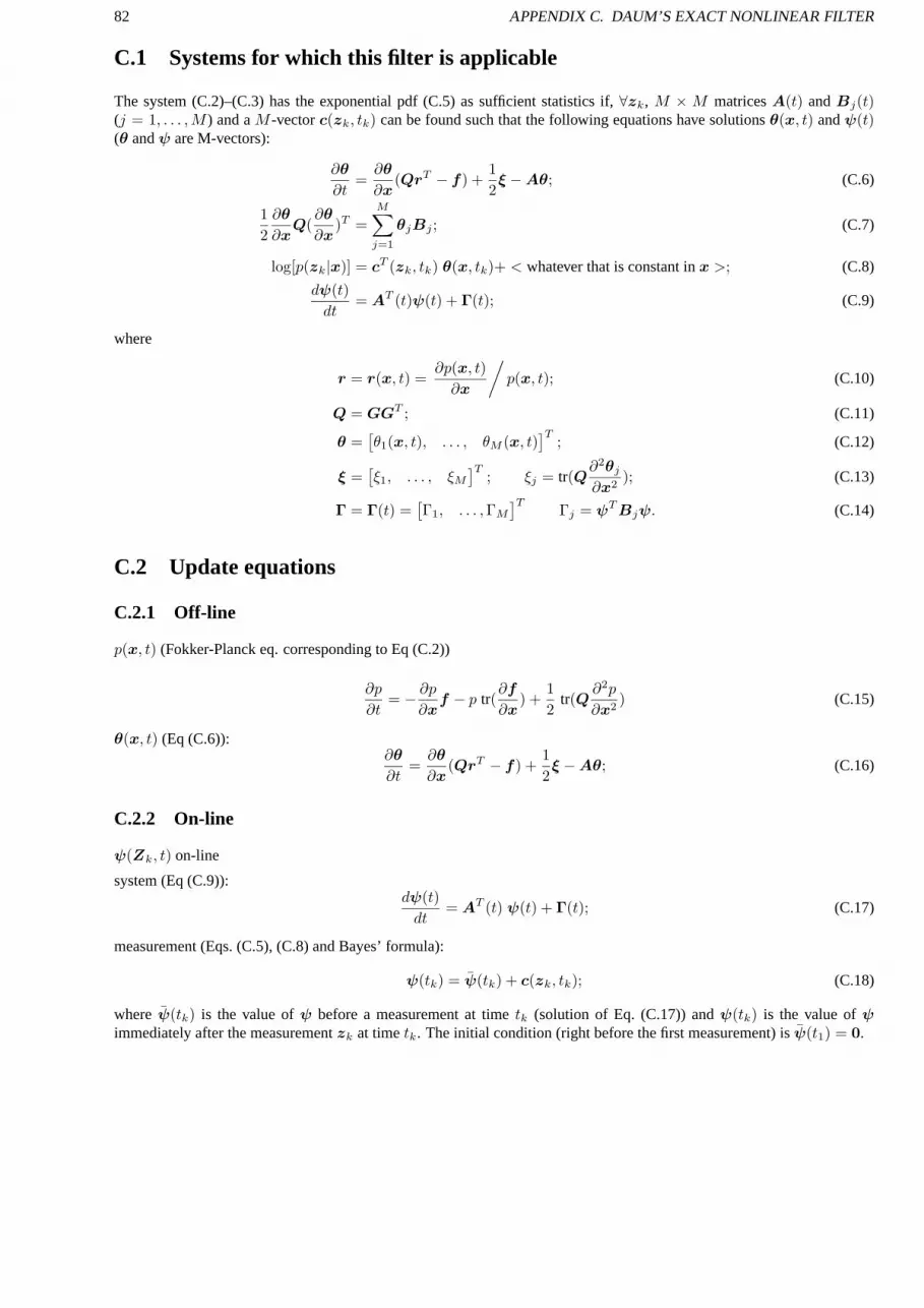
82 APPENDIX C. DAUM’S EXACT NONLINEAR FILTER

C.1 Systems for which this filter is applicable

The system (C.2)–(C.3) has the exponential pdf (C.5) as sufficient statistics if,∀zk, M × M matricesA(t) andBj(t)(j = 1, . . . ,M ) and aM -vectorc(zk, tk) can be found such that the following equations have solutionsθ(x, t) andψ(t)(θ andψ are M-vectors):

∂θ

∂t=∂θ

∂x(QrT − f) +

1

2ξ −Aθ; (C.6)

1

2

∂θ

∂xQ(

∂θ

∂x)T =

M∑

j=1

θjBj ; (C.7)

log[p(zk|x)] = cT (zk, tk) θ(x, tk)+ < whatever that is constant inx >; (C.8)

dψ(t)

dt= AT (t)ψ(t) + Γ(t); (C.9)

where

r = r(x, t) =∂p(x, t)

∂x

/

p(x, t); (C.10)

Q = GGT ; (C.11)

θ =[

θ1(x, t), . . . , θM (x, t)]T

; (C.12)

ξ =[

ξ1, . . . , ξM]T

; ξj = tr(Q∂2θj

∂x2); (C.13)

Γ = Γ(t) =[

Γ1, . . . ,ΓM

]TΓj = ψTBjψ. (C.14)

C.2 Update equations

C.2.1 Off-line

p(x, t) (Fokker-Planck eq. corresponding to Eq (C.2))

∂p

∂t= − ∂p

∂xf − p tr(

∂f

∂x) +

1

2tr(Q

∂2p

∂x2) (C.15)

θ(x, t) (Eq (C.6)):∂θ

∂t=∂θ

∂x(QrT − f) +

1

2ξ −Aθ; (C.16)

C.2.2 On-line

ψ(Zk, t) on-line

system (Eq (C.9)):dψ(t)

dt= AT (t) ψ(t) + Γ(t); (C.17)

measurement (Eqs. (C.5), (C.8) and Bayes’ formula):

ψ(tk) = ψ(tk) + c(zk, tk); (C.18)

whereψ(tk) is the value ofψ before a measurement at timetk (solution of Eq. (C.17)) andψ(tk) is the value ofψimmediately after the measurementzk at timetk. The initial condition (right before the first measurement)is ψ(t1) = 0.

Appendix D

Particle filters

D.1 IntroductionFIXME:

chapter. Is itderiveAs mentioned in section 4.1, an assumption these filters makeis the Markov assumption. The observations are also assumed

to be conditionally independent given the state.

D.2 Joint a posteriori density

In the most general formulation, we want to estimate a characteristic of our joint a posteriori distributionPost (X(k))(eg. the mean value, what means thath (X) = X):

E [h (X) | Post (X(k))] =

∫

h (X(k))Post (X(k)) dX(k) (D.1)

with Post (X(k)) as defined in (2.4) on page 20 andE [f |p] denoting the expected value of the functionf under the pdfp.In a sampling based approach, we estimate the a posteriori distribution by drawingN samples of it

Post (X(k)) ≈ 1

N

N∑

i=1

δXik(Xk) (D.2)

whereXik denotes thei-th sample drawn fromPost (X(k)) andδ denotes the Dirac function.

D.2.1 Importance sampling

The goal of all particle filters is to estimate characteristics of Post (X(k)) by using samples drawn from it. Becausewe don’t knowPost (X(k)) (and even if we would know, it would be very hard to draw samples of it because of it’scomplex shape), we’ll useimportance sampling(see chapter 8) to approximate the posterior and we’ll take into account thedifferences by multiplying samples with their associated weights. This means that we’ll approximate the expected value ofeq. (D.1) as follows:

E [h (X(k)) | Post (X(k))] =

∫

h (X(k))Post (X(k)) dX(k)

=

∫

h (X(k))Post (X(k))

Prop (X(k))Prop (X(k)) dX(k)

(D.3)

whereProp (X(k)) is theproposal distribution. It’s a pdf with the same arguments aPost (X(k))(as defined in equation2.4), but it has a different “form”.

Suppose we denote a certain sample (instantiation) ofX(k) asXi(k) and the ratio between the value of the a posterioriand proposal pdf at that sample asw

(

Xi(k))

(orwi in a shortened version)

w(

Xi(k))

= wi =Post

(

Xi(k))

Prop(

Xi(k)) (D.4)

83

84 APPENDIX D. PARTICLE FILTERS

thenw (X(k)) is a function ofX(k) and equation D.3 becomes

E [h (X(k)) | Post (X(k))] =

∫

h (X(k))w (X(k))Prop (X(k)) dX(k) (D.5)

We can thus obtain an estimate of our expected value withN samples of our proposal distribution

E [h (X(k)) | Post (X(k))] ≈ 1

N

N∑

i=1

h(

Xi(k))

w(

Xi(k))

(D.6)

Hier klopt iets niet met diewaarom dit niet mag en

vervangen moet worden doorenormaliseerde gewichten

This still doesn’t allow for a recursive solution of our problem. Indeed, at a certain timestepk, this means we should choosea proposal density and sampleN × k samples of dimensionRn of this proposal density. If however, we would be ableto formulate our problem in a recursive way, this would allowus to keep the number of samples we have to generate at acertain time instant constant (N ).

Remark D.1 Note that this approach leaves us with samples of thejoint a posteriori density! It can be proved that, providedthat enough samples are drawn, by taking the last vector of each of these samples, one obtains samples of the marginal pdf!

Remark D.2 Note that there also exist particle filters that use other Monte Carlo sampling methods than importance sam-pling. Markov chain Monte Carlo methods are often to computationally complex but rejection methods [16] are also used!

D.2.2 Sequential importance sampling (SIS)

Obtaining the joint a posteriori distribution in a recursiv e way

To avoid to heavy notation, we’ll combine some symbols as we already did before (see section 2.4, remark 2.10 on page21).

Hk−1 =[

uk−1 θf fk−1

]

(D.7)

Ik =[

sk θg gk

]

(D.8)

With these symbols, we refrase the 3 most important equations for Markov Systems (2.5, 2.6, 2.7 from section 2.4) on page20 here for thejoint a posterioridensity:

Remark D.3 Note that the prediction step does not contain an integral here . Note also that we can formulate the iterationFIXME: explain!

step here as a simpleproductof distributions, and do not really have to make the two-stepapproach.prediction-recursion!

Post (X(k)) = P(

X(k)∣

∣Post (X(k − 1)) ,Hk−1, Ik,zk

)

We can obtain the this in a recursive way, using Bayes’ rule and the Markov assumption:

P ( X(k) = Xk

∣

∣Post (X(k − 1)) ,Hk−1, Ik,zk

)

=P (zk |Xk, Post (X(k − 1)) ,Hk−1, Ik)P (Xk | Post (X(k − 1)) ,Hk−1, Ik)

P (zk | Post (X(k − 1)) ,Hk−1, Ik)

=P (zk | xk, Ik)P (Xk | Post (X(k − 1)) ,Hk−1, Ik)

P (zk | Post (X(k − 1)) ,Hk−1, Ik)

=P (zk | xk, Ik)P (Xk−1,xk | Post (X(k − 1)) ,Hk−1, Ik)

P (zk | Post (X(k − 1)) ,Hk−1, Ik)

=P (zk | xk, Ik)P (xk |Xk−1, Post (X(k − 1)) ,Hk−1, Ik)P (Xk−1 | Post (X(k − 1)) ,Hk−1, Ik)

P (zk | Post (X(k − 1)) ,Hk−1, Ik)

=P (zk | xk, Ik)P (xk | xk−1,Hk−1)Post (X(k − 1))

P (zk | Post (X(k − 1)) ,Hk−1, Ik)

= Post (X(k − 1))P(

zk

∣

∣xk, Ik

)

P (xk|xk−1,Hk−1)

P (zk)

(D.9)

And thus we obtain the following recursive formula forPost (X(k)):The last line of equationcorrect! The denominator

to the probability of themeasurement “tout court”) Post (X(k)) = Post (X(k − 1))

P(

zk

∣

∣xk, Ik

)

P (xk|xk−1,Hk−1)

P (zk)(D.10)

D.3. THEORY VS. REALITY 85

Obtaining the Proposal distribution in a recursive way

PROOF Suppose we dispose ofS samples of a pdfp(x) xi, i = 1 → S . For each of these samples, we know the pdfp(y|x = xi) and we can sample from this distribution (and thus obtainingyi). Can we combine thexi andyi to obtainsamples of the joint pdfp(x, y) = p(y|x)p(x)?

If the above can be proved , this allows us to solve the problemrecursively. Indeed, (see also eq. (2.1) on page 19) FIXME: The pr5 of the algoritmic

Prop (X(k)) = Q(

X(k) = Xk

∣


= Q(

Xk−1,xk

∣


= Q(

xk

∣

∣Xk−1,Zk, . . . , P (x(0)))

Q (Xk−1|Zk, . . . , P (x(0)))

= Q(

xk

∣

∣xk−1,zk,Hk−1, Ik))

Prop (X(k − 1))

(D.11)

We can thus recursively use this formula to start from ana priori proposal distribution

Combining those 2

Starting from the definition of the weights (D.4), and using both formulas for the recursion of the proposal density (D.11)and the a posteriori density (D.10), we obtain

w(

Xi(k))

=Post

(

Xi(k))

Prop(

Xi(k))

=Post

(

Xi(k − 1)) P (zk|xk,Ik)P (xk|xk−1,Hk−1)

P (zk)

Prop(

Xi(k − 1))

Q(

xk

∣

∣xk−1,zk,Hk−1, Ik

)

= αw(

Xi(k − 1)) P (zk | xk, Ik)P (xk | xk−1,Hk−1)

Q(

xk

∣


)

(D.12)

The unknown normalizing factorα = 1P (zk) is a serious problem, or not? Indeed, this factor is not dependent of the

estimated state vector and can thus be put before the integral in eq. (D.5).

We can avoid the unknown normalizing factorα by working with normalized weightsw(

Xi(k))

w(

Xi(k))

=w(

Xi(k))

∑Ni=1 w

(

Xi(k))

(D.13)

This results in algorithm 8.

Algorithm 8 Generic Particle filter algorithmSampleN samples from the a priori densityfor i = 1 toN do

Samplexik fromQ

(

xk

∣


)

Assign the particle a weight according to Eq. (D.12)end for

D.3 Theory vs. realityFIXME: This isof this text, as youAfter a few iteration steps, one (of few) of the weights becomes very large (or near to one), whileas the other weights

become negligible. This is called theDegeneracy phenomenon. There are 2 solutions for this:Resamplingand a goodchoice of the proposal density (You did notice we didn’t tell you anything yet about the choice of the proposal density,didn’t you? ).

This last issue (the choice of the proposal density) is not only important to avoid degeneracy, it also strongly influences thevariance of the sample weights and thus the convergence of the filter!

86 APPENDIX D. PARTICLE FILTERS

D.3.1 Resampling (SIR)

. Discuss basic resampling and thesample impoverishmentproblem.and next section shouldstill be written

Resampling can be done inO(N).FIXME: include algorithm

D.3.2 Choice of the proposal density

Discuss the ideal (minimal variance) choice: [38]. In reality almost never possible! . Some other variants areFIXME: include a number ofvariants and describe them

• The auxiliary particle filter [91]

• Regularized particle filter [84]

D.4 Literature

• The SMC homepage1 has lots of useful links to papers, videos, software . . .

• Good tutorials: [6]

• Arnaud Doucet and others have written several interesting papers [40, 38] and books [39, 37] about particle filters

• Sebastian Thrun and others have written several papers about the application of Particle filters in applications [81, 79,35].

• . . .FIXME: update this!

D.5 Software

• The Bayesian Filtering Library (BFL)2 of Klaas Gadeyne contains (amongst others) C++ support for particle filters.

• The Player Stage Project3 has an particle filter implementation in C for mobile robotFIXME: check this

• Bayes++4 also contains an implementation of a SIR filter (and several other “schemes” for Bayesian filtering)

1http://www-sigproc.eng.cam.ac.uk/smc/2http://people.mech.kuleuven.ac.be/˜kgadeyne/bfl.html3http://playerstage.sourceforge.net/4http://www.acfr.usyd.edu.au/technology/bayesianfilter/Bayes++.htm

Appendix E

The EM algorithm, M-step, proofs

FIXME:noodzakelijkThe M-step of the EM-algorithm calculates aθ = θk that increasesQ(θ,θk−1), (Eq. (5.3) or Eq. (5.4)). This estimate

will guarantee an increase in the (incomplete-data) likelihood function Eq. (5.2). Proof is given here.

For the ease of notation “Uk−1,Sk,F k−1,Gk, P (X(0))” is abbreviated asHk.

Proof: part oneIn this paragraph, we prove that,∀θk,

E[

log(

p(

X(k)∣

∣Zk,Hk,θk)) ∣

∣

∣Zk,Hk,θ

k−1]

−E[

log(

p(

X(k)∣

∣Zk,Hk,θk−1)) ∣

∣

∣Zk,Hk,θ

k−1]

≤ 0.

E[

log(

p(

X(k)∣

∣Zk,Hk,θk)) ∣

∣

∣Zk,Hk,θ

k−1]

− E[

log(

p(

X(k)∣


∣

∣Zk,Hk,θ

k−1]

=

∫

[

log(

p(

X(k)∣

∣Zk,Hk,θk))

− log(

p(

X(k)∣

∣Zk,Hk,θk−1)) ]

p(

X(k)∣

∣Zk,Hk,θk−1)

dX(k);

=

∫

[

logp(

X(k)∣

∣Zk,Hk,θk)

p(

X(k)∣

∣Zk,Hk,θk−1)

]

p(

X(k)∣

∣Zk,Hk,θk−1)

dX(k)

becauselog(x) ≤ x− 1, ∀x,

≤∫

[ p(

X(k)∣

∣Zk,Hk,θk)

p(

X(k)∣

∣Zk,Hk,θk−1) − 1

]

p(

X(k)∣

∣Zk,Hk,θk−1)

dX(k)

=

∫

p(

X(k)∣

∣Zk,Hk,θk)

dX(k)−∫

p(

X(k)∣

∣Zk,Hk,θk−1)

dX(k)

= 0.

Proof: part twoIn this paragraph we show that aθk that increasesQ(θ,θk−1), will increase the logarithm of the (incomplete-data)

likelihood function,

log(

p(

Zk

∣

∣Hk,θk))

> log(

p(

Zk

∣

∣Hk,θk−1))

; (E.1)

hence it will increase the (incomplete-data) likelihood function itself (Eq (5.2)).

We know thatp(

X(k),Zk

∣

∣Hk,θ)

= p(

X(k)∣

∣Zk,Hk,θ)

p(

Zk

∣

∣Hk,θ)

;

hence:log(

p(

Zk

∣

∣Hk,θ))

= log(

p(

X(k),Zk

∣

∣Hk,θ))

− log(

p(

X(k)∣

∣Zk,Hk,θ))

.

87

88 APPENDIX E. THE EM ALGORITHM, M-STEP, PROOFS

When averaging overX, given the in the E-step calculated pdfp(

X(k)∣

∣Zk,Hk,θk−1)

, this becomes (the term on the

left side is independant ofX(k)):

log(

p(

Zk

∣

∣Hk,θ)

)

=

E[

log(

p(

X(k),Zk

∣

∣Hk,θ))

∣

∣

∣Zk,Hk,θ

k−1]

− E[

log(

p(

X(k)∣

∣Zk,Hk,θ))

∣

∣

∣Zk,Hk,θ

k−1]

.

Hence the change in Eq. (E.1) between two updates is:

log(

p(

Zk

∣

∣Hk,θk)

)

− log(

p(

Zk

∣

∣Hk,θk−1)

)

=

E[

log(

p(

X(k),Zk

∣

∣Hk,θk)) ∣

∣

∣Zk,Hk,θ

k−1]

− E[

log(

p(

X(k),Zk

∣

∣Hk,θk−1)) ∣

∣

∣Zk,Hk,θ

k−1]

− E[

log(

p(

X(k)∣

∣Zk,Hk,θk)) ∣

∣

∣Zk,Hk,θ

k−1]

+E[

log(

p(

X(k)∣


∣

∣Zk,Hk,θ

k−1]

.

The first two terms on the right hand side equalQ(θk,θk−1) −Q(θk−1,θk−1). When Eq. (5.3) or Eq. (5.4) is satisfied,this is strict positive. Part one of the proof showed that thelast two terms on the right hand side give a positive sum, forall values ofθk. This makes that —if Eq. (5.3) or Eq. (5.4) is satisfied— the left hand side is positive, i.e.θk increasesthe logarithm of the incomplete-data likelihood function,and hence increases also the incomplete-data likelihood functionitself (Eq. (5.2)).

Appendix F

Bayesian (belief) networks

FIXME:consists of someF.1 Introduction

Definition F.1 (Belief networks) (from [62]) Belief networks are a widely applicable formalism for compactly representingthe joint probability distribution over a set of random variables.

A Bayesian network provides a model representation for the joint distribution of a set of variables in terms of conditionaland prior probabilities, in which the orientations of the arrows represent influence (usually though not always of a causalnature), such that these conditional probabilities for these particular orientations are relatively straightforward to specify.When data are observed, then typically an inference procedure is required. This involves calculating marginal probabilitiesconditional on the observed data using Bayes’ theorem, which is diagrammatically equivalent to reversing one or more ofthe Bayesian network arrows.

Features:

• Conditional independence properties can be used to simplify the general factorization formula for the joint probability.In some cases, this can be very important to provide an efficient basis for the implementation of some MCMC variantssuch asGibbs sampling[55].

• That result can be expressed by the use of a DAG

A Bayesian Network is adirected acyclic graph(DAG), whose structure defines a set ofconditional independence(oftendenoted as⊥⊥) properties. This follows from the fact that any PDF can be factorised

P (X1, . . . ,Xn) = P (X1 | X2 . . . Xn) . . . P (Xn−1 | Xn)P (Xn)

FIXME: Adddifference between

FIXME: Notation:

Recursive factorization:

P (X1, . . . ,Xn) =n∏

i=1

P (Xi|parents(Xi))

Marginalising over achildlessnode is equivalent to simply removing it and any edges to it from its parents.

Directed acyclic graphs can always have their nodes linearly ordered so that for each nodeX all of its parentsPa(X)precedes it in the ordering. This is called atopological ordering. FIXME:

Directed Markov property

A variable is conditionally independent of its non-descendents given its parents:

X ⊥⊥ nd(X) | parents(X)

wherend(X) denotes the non-descendents ofX.

Undirected graphical models, also called Markov Random Fields (MRFs)

F.2 Inference in Bayesian networks

89

90 APPENDIX F. BAYESIAN (BELIEF) NETWORKS

Appendix G

Entropy and information

The concept of entropyH arises from an equally important concept called(self)-informationI. The following sectionsdefine these concepts and the relation between them. A good book on this subject is [29].

G.1 Shannon entropy

Shannon [106, 107] defined a measure of the “amount of uncertainty” or “the amount of chaos” or “the lack of information”represented by a probability distribution: theShannon entropyor informational entropy.

Shannon looked for a measure of uncertainty of a discrete probability distribution (p(x = x1) = p1, . . ., p(x = xn) = pn)with the following properties [106, 107]:

• H should be continuous in thepi

• If all the pi are equal,pi = 1/n, thenH should be a monotonic increasing function ofn. With equally likely eventsthere is more choice, or uncertainty, when there are more possible events.

• If a choice is broken down into two successive choices, the originalH should be the weighted sum of the individualvalues ofH. e.g. three possible values,p1 = 1

2 , p2 = 13 , andp3 = 1

6 ,H( 12 ,

13 ,

16 ) = H( 1

2 ,12 ) + 1

2H( 23 ,

13 )

[106, 107] prove that the onlyH satisfying the three above assumptions is of the form:

H(x) = −Kn∑

i=1

pi log pi (G.1)

whereK is a positive constant. Shannon defined entropy as

H(x) = −n∑

i=1

pi log pi = E[− log p(x)] (G.2)

where any choice of “log” is possible; this changes only the units of the entropy result (e.g. log: [bits], ln: [nats]). He alsoextended this to the continuous case (differential entropy):

H(x) = −∫ ∞

−∞

p(x) log p(x)dx = E[− log p(x)] (G.3)

e.g. for a Gaussian distribution1 (d dimensional state):

p(x) =1

√

(2π)d|P |e−

1

2(x−µ)TP−1(x−µ) (G.4)

H(x) = log

(

√

(2πe)d|P |)

=1

2log(

(2πe)d|P |)

(G.5)

1The Gaussian distribution has an important special entropy characterization: under the assumption of a fixed covariance matrix, the function thatmaximizes the entropy is Gaussian [106, 107].

91

92 APPENDIX G. ENTROPY AND INFORMATION

where|P | is the determinant of the covariance matrix.

There is one important difference between the entropy of continuous and discrete distributions. In the discrete case, theentropy measures the randomness of the chance variable in anabsoluteway. In the continuous case, the measurement isrelative to the coordinate system: this means that if we change the coordinates, the entropy will change. The entropy inthe continuous case can be considered as a measure of randomness relative to an assumed standard, namely the coordinatesystem chosen with each small volume elementdx1 . . . dxn given equal weight. As the scale of measurements is set to anarbitrary zero corresponding to an uniform distribution over this unit volume, the entropy of a continuous distribution canbe negative. Differences between two entropies of the pdf expressed in the same coordinate system, however, do not dependon the choice of this coordinate frame.

G.2 Joint entropy

The joint entropy is defined as the entropy of the joint distribution.For discrete distributions:

H(x,y) = −∑

X

∑

Y

p(x,y) log p(x,y) (G.6)

X andY define all possible values forx andy.For continuous distributions:

H(x,y) = −∫

X

∫

Y

p(x,y) log p(x,y)dydx (G.7)

G.3 Conditional entropy

The conditional entropy isnot the entropy of the posterior conditional distributionp(y|x = xk), instead it is defined as:For discrete distributions:

H(y|x) = −∑

X

∑

Y

p(x,y) log p(y|x) = −∑

X

∑

Y

p(x,y) logp(x,y)

p(x)(G.8)


H(y|x) = −∫

X

∫

Y

p(x,y) log p(y|x)dxdy = −∫

X

∫

Y

p(x,y) logp(x,y)

p(x)dxdy (G.9)

Some (in)equalities related to the conditional entropy are:

H(x,y) = H(x) +H(y|x) = H(y) +H(x|y) (G.10)

H(y|x) 6= H(x|y) (G.11)

H(x,y|z) = H(x|z) +H(y|x,z) (G.12)

H(y|x) ≤ H(y) (G.13)

G.4 Relative entropy

The concept ofrelative entropyis also known under the nameKullback-Leibler informationor Kullback-Leibler dis-tance[69, 68], mutual entropy, informational divergence, information for discriminationor cross entropy. It representsa measure for the goodness of fit or closeness of two distributionsp1(x) andp2(x):

D(p2(x)||p1(x)) = E[logp2(x)

p1(x)]; (G.14)

For discrete distributions:

D(p2(x)||p1(x)) =n∑

i=1

p2(x) logp2(x)

p1(x)(G.15)

=

n∑

i=1

p2(x) log p2(x)−n∑

i=1

p2(x) log p1(x) (G.16)

G.5. MUTUAL INFORMATION 93


D(p2(x)||p1(x)) =

∫ ∞

−∞

p2(x) logp2(x)

p1(x)dx (G.17)

=

∫ ∞

−∞

p2(x) log p2(x)dx−∫ ∞

−∞

p2(x) log p1(x)dx (G.18)

Note: not symmetric !:

D(p2(x)||p1(x)) 6= D(p1(x)||p2(x)) (G.19)

G.5 Mutual information

Mutual informationI(x,y) is the reduction in the uncertainty ofx due to the knowledge ofy.For discrete distributions:

I(x,y) =∑

X

∑

Y

p(x,y) logp(x,y)

p(x)p(y)(G.20)

= D(p(x,y)||p(x)p(y)) (G.21)


I(x,y) =

∫ ∞

−∞

∫ ∞

−∞

p(x,y) logp(x,y)

p(x)p(y)dxdy (G.22)

= D(p(x,y)||p(x)p(y)) (G.23)

I(x,y) is always positive:I(x,y) ≥ 0.

x says as much abouty asy says aboutx:

I(x,y) = I(y,x) (G.24)

The relation between entropy and mutual information is (seefigure G.1):

I(x,y) = H(x)−H(x|y) (G.25)

= H(y)−H(y|x) (G.26)

= H(x) +H(y)−H(x,y) (G.27)

G.6 Principle of maximum entropy

Principle of maximum entropy [60]: When making inferences based on incomplete information, the pdf with maximumentropy is the least biased estimate possible on the given information; i.e. it is maximally noncommittal with regard tomissing information.

The intuition is that we should make the least possible additional assumptions aboutp.

It turns out that there is always a unique maximal entropy measure.

G.7 Principle of minimum cross entropy

Principle of minimum cross entropy [69, 68]: The Shannon entropy is maximum when the pdf of the random variableis that one which is as close to the prior distribution as possible. This is equivalent to maximizing the Shannon entropy(section G.6).

94 APPENDIX G. ENTROPY AND INFORMATION

H(x) H(y)

H(x,y)

H(x|y) H(y|x)I(x,y)

Figure G.1: Relation between entropy and mutual information

G.8 Maximum likelihood estimation

The maximum likelihood estimation is equivalent to the minimum Kullback-Leibler distance estimation:

x = minxD(p(Zk)||p(Zk|x)) (G.28)

i.e. the maximum likelihood estimation (or the maximum a posteriori probability estimation) is looking for a pointx, whichis not necessarily unique, that minimizes the Kullback-Leibler distance betweenp(Zk|x) and the empirical distributionp(Zk) (possibly modified by the prior).

Appendix H

Fisher information matrix and Cram er-Raolower bound

The inverse of the Fisher information matrix determines a lower bound on the covariance matrix of the estimate that canbe obtained with an efficient estimator, given the measurements. Note that the covariance matrix is a good measure of theuncertainty on the estimate if we are interested in a single value estimate: with the expected value of the distribution asestimate, the covariance matrix expresses the covariance of the deviations between this estimate and the real value1. Fora multimodal distribution with small peaks, the covariancematrix will be large, in contrast to the entropy measures whichwill be small. If, on the other hand, we are not interested in asingle value estimate e.g. because our estimate is intrinsicallymultimodal, the covariance matrix measure is not a good measure.

The next section describes the Fisher information matrix and Cramer-Rao lower bound for the estimation of anon randomstate vector, Section H.2 for arandomstate vector. The original derivation of the Fisher information matrix and the Cramer-Rao lower bound is made for the non random case: given a numberof measurements, we want to estimate a static state(parameter)x. The random case is an extension to Bayesian estimation: given a number of measurementsand an a prioridistribution of the statex, we want to estimate the statex. The extension is also valid fordynamic states, changing in timeaccording to a process function with process uncertainty.

For more info, see [120].

H.1 Non random state vector estimation

H.1.1 Fisher information matrix

TheFisher information matrix[48] for a non random state (parameter) vector is defined as the covariance of the gradient ofthe log-likelihood, that is:

I(x) = E[

(Ox ln p(Zk|x))(Ox ln p(Zk|x))T]

(H.1)

= −E[

OxOTx ln p(Zk|x)

]

(H.2)

WhereOx = [ ddx1

. . . ddxn

]T is the gradient operator with respect tox = [x1 . . .xn], andOxOTx is the Hessian matrix.

E[.] is the expected value with respect top(Zk|x). This measure was introduced by Fisher as a measure of the amount ofinformation aboutx, present in the measurements. The elements of the matrixI(x) are:

Iij(x) = E

[

−∂2 ln p(Zk|x)

∂xi∂xj

]

(H.3)

H.1.2 Cramer-Rao lower bound

The inverse of the Fisher Information Matrix, also called the Cramer-Rao lower boundis a lower bound on the covariancematrix2 for an unbiased estimatorT (x) of x [43, 95, 30] :

var(T ) ≥ I−1(x∗). (H.4)

1Note that this is the estimate which has the smallest covariance of the deviations to the real state.2The assumption of the normality of the estimate is not necessary.

95

96 APPENDIX H. FISHER INFORMATION MATRIX AND CRAMER-RAO LOWER BOUND

I(x∗) is the Fisher information matrix evaluated at thetruestate vectorx∗. The matrixinequality (H.4) means thatvar(T )−I−1(x∗) is positive semi definite. The bound above depends on the actual state value. Hence, it is not possible to computethe bound in any real estimation cases where the states are unknown. However, the bound can be used to analyse andevaluate estimators in simulations.

The unbiased estimatorT (x) is efficientif var(T ) = I−1(x∗). Note that it is possible that there does not exist an estimatormeeting this lower bound.

H.2 Random state vector estimation

The Fisher information matrix as defined above, is for the estimation of the non random state. In the Bayesian approachto estimation, the state vector israndom(uncertain) with an apriori probability distribution. Thedefinition of the Fisherinformation matrix is extended to this case and, as was the case for the estimation of non random states, the inverse of thisFisher information matrix is also the Cramer-Rao lower bound for the mean square error [120, 117].

H.2.1 Fisher information matrix

The Fisher information matrix for a random state vectorxk is defined as the covariance of the gradient of the total log-probability, that is:

Ik|k = E[

(Oxkln p(xk,Zk))(Oxk

ln p(xk,Zk))T]

(H.5)

= −E[

OxkOTxk

ln p(xk,Zk)]

(H.6)

i.e. the elements of the matrixIk|k are

Ik|k,ij = E[−∂2 ln p(Zk,xk)

∂xk,i∂xk,j] (H.7)

The meanE[.] is taken over the distributionp(xk,Zk).

H.2.2 Alternative expressions for the information matrix

• Ik|k can be divided intoIk|k,D andIk|k,P (provided that these exists):

Ik|k = −E[

OxkOTxk

ln p(xk,Zk)]

; (H.8)

Ik|k,D + Ik|k,P = E[

−OxkOTxk

ln p(Zk|xk)]

+ E[

−OxkOTxk

ln p(xk)]

(H.9)

Ik|k,D is the information obtained from the data,Ik|k,P represents the information in the prior distributionp(xk).

• The information matrix can also be described in function of the posterior distributionp(xk|Zk):

Ik|k = −OxkOTxk

ln p(xk,Zk); (H.10)

= E[

−OxkOTxk

ln p(xk|Zk)]

+ E[

−OxkOTxk

ln p(Zk)]

; (H.11)

= E[

−OxkOTxk

ln p(xk|Zk)]

(H.12)

• A recursive formulation is possible for Markovian models:

p(Zk,xk) = p(Zk−1,xk)p(zk|xk) (H.13)

Ik|k = Ik|k−1 − E[

OxkOTxk

ln p(zk|xk)]

(H.14)

H.2.3 Cramer-Rao lower bound

The Cramer-Rao bound for a random state vectorxk is called theVan Trees version of the Cramer-Rao bound, or theposterior Cramer-Rao bound[117]. As was the case for the estimation of non random states, the Cramer-Rao lower boundis the inverse of the Fisher information matrixIk|k.

H.3. ENTROPY AND FISHER 97

H.2.4 Example: Gaussian distribution

If p(xk|Zk) is Gaussian:

Ik|k = E[

−OxkOTxk

ln p(xk|Zk)]

(H.15)

= E

[

−OxkOTxk

(c0 −1

2(xk − µk))TP−1

k (xk − µk))

]

(H.16)

= E[

P−1k

]

(H.17)

If we obtain anefficientestimator forxk, the Fisher information will simply be given by the inverse of the error covariancematrix of the state :Ik|k = P−1

k .

H.2.5 Example: Kalman Filtering

For a linear system model, the Fisher information will be given by the Kalman Filter formulas for the covariance matrixIk|k = P−1

k .

For a nonlinear system model, the Fisher information will begiven by the Extended Kalman Filter formulas for the covari-ance matrixif all derivatives are evaluated at thetruestate value.

H.2.6 Example: Cramer-Rao lower bound on a part of the state vector

Assume that the state vectorxk is decomposed into two partsxk = [xTk,αx

Tk,β ]T , and the information matrixIk|k is

correspondingly decomposed into blocks

Ik|k =

[

Iαα Iαβ

Iβα Iββ

]

; (H.18)

then, assuming thatI−1αα exists, the covariance matrix of the estimate ofxk,β is

P k,β ≥ Iββ − IβαI−1ααIαβ . (H.19)

H.3 Entropy and FisherFIXME: dezede klok horenthere is a relation between entropy and the Fisher information matrix, namely thede Bruijn’s identity. If x is a random

variable, with finite variance and pdfp(x); andy is an independently normally distributed random variable with mean 0 andvariance 1:

∂

∂tHe(x+

√ty) =

1

2I(x+

√ty) (H.20)

If the limit exists ast→ 0:∂

∂tHe(x+

√ty)

∣

∣

∣

∣

t=0

=1

2I(x) (H.21)

Fisher represents the local behaviour of the relative entropy: it indicates the rate of change in information in a given directionof the probability manifold. For two distributionsp(z|x) andp(z|x′) [68]:

D(p(z|x)||p(z|x′)) ∼ 1

2I(x)(x− x′)2; (H.22)

I(x) =∑

X

p(z|x)( ∂∂x

ln p(z|x))2 (H.23)

98 APPENDIX H. FISHER INFORMATION MATRIX AND CRAMER-RAO LOWER BOUND

Bibliography

[1] H. Aikake. Information theory and an extension of the maximum likelihood principle. In B. Petrov and F. Csaki,editors,Proceedings of the Second International Symposium in Information Theory, pages 267–81. Akademiai Kiado,Budapest, Hungary, 1973.

[2] H. Aikake. A new look at the statistical model identification. IEEE Transactions on Automatic Control, 19:716–23,1974.

[3] H. Aikake. On the entropy maximiztion principle. In P. Krishniah, editor,Applications of Statistics, pages 27–41.North-Holland, Amsterdam, 1977.

[4] H. Aikake. Prediction and entropy. In A. Atkinson and S. Fienberg, editors,A Celebration of Statistics, pages 1–24.Springer, New York, 1985.

[5] D. Alspach and H. Sorenson. Nonlinear bayesian estimation using gaussian sum approximations.IEEE Transactionson Automatic Control, 17(4):439–448, August 1972.

[6] M. S. Arulampalam, S. Maskell, N. Gordon, and T. Clapp. A Tutorial on Particle Filters for Online Nonlinear/Non-gaussian Bayesian Tracking.IEEE Transactions on Signal Processing, 50(2):174–188, february 2002.http://www-sigproc.eng.cam.ac.uk/˜sm224/ieeepstut.ps .

[7] K. J. Astrom. Optimal control of markov decision processes with incomplete state estimation.J. Math. Anal. Appl.,10:174–205, 1965.

[8] Bar-Shalom and X. Li.Estimation and Tracking: Principles, Techniques and Software. Artech House, 1993.

[9] A. Barto, S. Bradtke, and S. Singh. Learning to act using real-time dynamic programming.Artificial Intelligence,72:81–138, 1995.

[10] R. Bellman.Dynamic Programming. Princeton University Press, Princeton, New Jersey, 1957.

[11] R. Bellman. A markov decision process.Journal of Mathematical Mechanics, 6:679–684, 1957.

[12] V. Beneˇ s. Exact finite-dimensional filters for certaindiffusions with nonlinear drift.Stochastics, 5:65–92, 1981.

[13] J. M. Bernardo and A. F. M. Smith.Bayesian Theory. Wiley series in probability and statistics. John Wiley & Sons,repr. edition, 2001.

[14] D. P. Bertsekas.Dynamic Programming and Optimal Control, Volume I. Athena Scientific, Belmont Massachusetts,1995.

[15] D. P. Bertsekas.Dynamic Programming and Optimal Control, Volume II. Athena Scientific, Belmont Massachusetts,1995.

[16] E. Bølviken, P. Acklam, N. Christophersen, and J.-M. Størdal. Monte Carlo filters for non-linear state estimation.Automatica, 37(2):177–183, 2001.http://www.math.uio.no/˜erikb/automatica.pdf .

[17] B. Bonet and H. Geffner. Planning with incomplete information as heuristic search in belief space. InProc. of the5th International Conference on AI PLanning and Scheduling,AAAI Press, pages 52–61, Colorado, 2000.

[18] B. Bonet and H. Geffner. Planning as heuristic search.Artificial Intelligence, Special issue on Heuristic Search,129(1–2):5–33, 2001.

[19] C. Boutilier, T. Dean, and S. Hanks. Decision-theoretic planning: Structural assumptions and computational leverage.Journal of Artificial Intelligence Research, 11:1–94, 1999.

99

100 BIBLIOGRAPHY

[20] C. Boutilier and D. Poole. Computing optimal policies for partially observable decision processes using compactrepresentations.AAA, 2:1168–1175, 1996.

[21] S. Boyd and L. Vandenberghe.Convex Optimization. http://www.ee.ucla.edu/∼vandenbe/publications.html. Coursereader for EE364 (Stanford) and EE236B (UCLA), and draft of abook that will be published in 2003.

[22] G. Calafiore, M. Indri, and B. Bona. Robot dynamic calibration: Optimal trajectories and experiment al parameterestimation.IEEE Trans. on AC, 13(5):730–740, 1997.

[23] G. Casella and E. I. George. Explaining the Gibbs Sampler. The American Statistician, 46(3):167–174, 1992.

[24] A. Cassandra, L. Kaelbling, and J. Kurien. Acting UnderUncertainty: Discrete Bayesian Models for Mobile-RobotNavigation,. InProceedings of IEEE/RSJ International Conference on Intelligent Robots and Systems, 1996.http://www.cs.brown.edu/people/lpk/iros96.ps .

[25] A. R. Cassandra. Optimal policies for partially observable markov decision processes. Tech-nical Report CS-94-14, Brown University, Department of Computer Science, Providence RI,http://www.cs.brown.edu/publications/techreports/reports/CS-94-14.html 1994.

[26] A. R. Cassandra.Exact and approximate algorithms for partially observableMarkov decision processes. PhD thesis,U. Brown, 1998.

[27] H.-T. Cheng. Algorithms for Partially Observable Markov Decision Processes. PhD thesis, University of BritishColumbia, British Columbia, Canada, 1988.

[28] S. Chib and E. Greenberg. Understanding the Metropolis–Hastings Algorithm.The American Statistician, 49(4):327–335, 1995.

[29] T. M. Cover and J. A. Thomas, editors.Elements of Information Theory. Wiley Series in Telecommunications.Wiley-Interscience, 1991.

[30] H. Cramer. Mathematical methods of Statistics. Princeton. Princeton University Press, New Jersey, 1946.

[31] F. Daum. The fisher-darmois-koopman-pitman theorem for random processes. InProc. of the 1986 IEEE Conferenceon Decision and Control, pages 1043–1044.

[32] F. Daum. Solution of the zakai equation by separation ofvariables.IEEE Trans. Autom. Control. AC-32(10), 1987.

[33] F. Daum. New exact nonlinear filters. In e. J. C. Spall, editor, Bayesian Analysis of Time Series and Dynamic Models,chapter 8, pages 199–226. Marcel Dekker inc., New York, 1988.

[34] J. De Geeter.Constrained system state estimation and task-directed sensing. PhD thesis, K.U.Leuven, Departmentof Mechanical engineering, div. PMA, Celestijnenlaan 300B, 3001 Leuven, Belgium, 1998.

[35] F. Dellaert, D. Fox, W. Burgard, and S. Thrun. Monte carlo localization for mobile robots. InProceedings of theIEEE International Conference on Robotics and Automation (ICRA’99), Detroit, Michigan, 1999.

[36] F. d’Epenoux. Sur un probleme de production et de stockage dans l’aleatoire. Revue Francaise Recherche Opra-tionelle, 14:3–16, 1960.

[37] A. Doucet.Monte Carlo Methods for Bayesian Estimation of Hidden Markov Models. PhD thesis, Univ. Paris-Sud,Orsay, 1997. in french.

[38] A. Doucet. On Sequential Simulation-Based Methods forBayesian Filtering. Technical Report CUED/F-INFENG/TR.310, Signal Processing Group, Dept. of Engineering, University of Cambridge, 1998.

[39] A. Doucet, N. de Freytas, and N. Gordon, editors.Sequential Monte Carlo Methods in Practice. Statistics forengineering and information science. Springer–Verlag, january 2001.

[40] A. Doucet, S. Godsill, and C. Andrieu. On sequential monte carlo sampling methods for bayesian filtering.Statisticsand Computing, 10(3):197–208, 2000.

[41] A. Drake. Observation of Markov Processes Through a Noisy Chanel. PhD thesis, Massachusetts Institute of Tech-nology, Cambridge, Massachusetts, 1962.

[42] R. Dugad and U. Desai. A tutorial on Hidden Markov Models. Technical Report SPANN-96.1, Indian institute ofTechnology, dept. of electrical engineering, Signal Processing and Artificial Neural Networks Laboratory, Bombay,Powai, Mumbai 400 076 India, may 1996.http://vision.ai.uiuc.edu/dugad/newhmmtut.ps.gz .

BIBLIOGRAPHY 101

[43] D. Dugue. Applications des proprietes de la limite au sens du calcul des probabilitesa l’etude des diverses questionsd’estimation.Ecol. Poly., 3(4):305–372, 1937.

[44] J. N. Eagle. The optimal search for a moving target when the search path is constrained.Operations research,32(5):1107–1115, 1984.

[45] G. J. Erickson and C. R. Smith, editors.Maximum-Entropy and Bayesian Methods in Science and Engineering.Vol. 1: Foundations; Vol. 2: Applications, Dordrecht, The Netherlands, 1988. Kluwer Academic Publishers.

[46] H. J. S. Feder, J. J. Leonard, and C. M. Smith. Adaptive mobile robot navigation and mapping.International Journalof Robotics Research, 18(7):650–668, July 1999.

[47] V. Fedorov.Theory of optimal experiments. Academic press, New York, 1972.

[48] R. Fisher. On the mathematical foundations of theoretical statistics.Pilosophical Transactions of the Royal Society,A,, 222:309–368, 1922.

[49] M. Forster and E. Sober. How to tell when simpler, more unified, or less ad hoc theories will provide more accuratepredictions.British Joural for the Philosophy of Science, 45:1–35, 1994.

[50] D. Fox, W. Burgard, F. Dellaert, and S. Thrun. Monte carlo localization: Efficient position estimation for mobilerobots. InProceedings of the Sixteenth National Conference on Artificial Intelligence (AAAI’99), Orlando, FL, 1999.

[51] D. Fox, W. Burgard, and S. Thrun. Active markov localization for mobile robots. volume 25, pages 195–207, 1998.

[52] D. Fox, W. Burgard, and S. Thrun. Markov localization for mobile robots in dynamic environments.Journal ofArtificial Intelligence Research, 11, 1999.

[53] J. D. Geeter, J. D. Schutter, H. Bruyninckx, H. V. Brussel, and M. Decreton. Tolerance-weighted L-optimal experi-ment design: a new approach to task-directed sensing.Advanced Robotics, 13(4):401–416, 1999.

[54] A. E. Gelfland and A. F. M. Smith. Sampling-Based Approaches to Calculating Marginal Densities.Journal of theAmerican Statistical Association, 85(410):398–409, june 1990.

[55] W. R. Gilks, S. Richardson, and D. J. Spiegelhalter, editors. Markov Chain Monte Carlo in Practice. Chapman &Hall, London, first edition, 1996.

[56] W. K. Hastings. Monte Carlo sampling methods using Markov Chains and their applications.Biometrika, 57:97–107,1970.

[57] M. Hauskrecht. Value-function approximations for partally observable markov decision processes.Journal of Artifi-cial Intelligence Research, 13:33–94, 2000.

[58] R. A. Howard.Dynamic Programming and Markov Processes. The MIT Press, Cambridge, Massachusetts, 1960.

[59] R. Ihaka and R. Gentleman. R: A language for data analysis and graphics.Journal of Computational and GraphicalStatistics, 5(3):299–314, 1996.

[60] E. T. Jaynes. How does the brain do plausible reasoning?Technical Report 421, Stanford University MicrowaveLaboratory, 1957. Reprinted in [45, Vol. 1, p. 1–24].

[61] F. Jelinek.Statistical methods for speech recognition. MIT Press, 1997.

[62] M. I. Jordan, editor. Learning in Graphical Models. Adaptive Computation and Machine Learning. MIT Press,London, England, 1999. ISBN 0262600323.

[63] R. E. Kalman. A new approach to linear filtering and prediction problems. 82:34–45, 1960.

[64] M. H. Kalos and P. A. Whitlock.Monte Carlo methods, volume I: Basics ofWiley-intersience publications. Wiley,New York, 1986.

[65] S. Koenig and R. Simmons. Solving robot navigation problems with initial pose uncertainty using real-time heuristicsearch. InProceedings of the International Conference on Artificial Intelligence Planning Systems, pages 154–153,1998.

[66] S. Kristensen. Sensor planning with bayesian decisiontheory.Robotics and Autonomous Systems, 19:273–286, 1997.

102 BIBLIOGRAPHY

[67] G. J. A. Krose and R. Bunschoten. Probabilistic localization by appearance models and active vision. InIEEEconference on Robotics and Automation, Detroit, May 1999.

[68] S. Kullback.Information theory and statistics. New York, NY, 1959.

[69] S. Kullback and R. Leibler. On information and sufficiency. Annals of mathematical Statistics, 22:79–86, 1951.

[70] S. E. Levinson. Continuously Variable Duration HiddenMarkov Models for speech analysis. InInt. Conf. onAcoustics, Speech, and Signal Processing, volume 2, pages 1241–1244. AT&T Bell Lab., april 1986.

[71] S. E. Levinson. Continuously Variable Duration HiddenMarkov Models for speech recognition.Computer, Speechand Language, 1:29–45, 1986.

[72] M. L. Littman, A. R. Cassandra, and L. P. Kaelbling. Efficient dynamic-programming updates in partially observ-able markov decision processes. Technical Report CS-95-19, Brown University, Department of Computer Science,Providence RI, 1995.

[73] M. L. Littman, T. L. Dean, and L. P. Kaelbling. On the complexity of solving markov decision problems. InProceedings of the 11th International Conference on Uncertainty in Artificial Intelligence, 1995.

[74] W. S. Lovejoy. A survey of algorithmic methods for partially observed markov decision processes.Annals ofOperations Research, 18:47–65, 1991.

[75] D. J. C. MacKay. Information theory, inference and learning algorithms. Textbook in preparation.http://wol.ra.phy.cam.ac.uk/mackay/itprnn/ , 1999.

[76] N. Metropolis, A. W. Rosenbluth, M. N. Rosenbluth, A. H.Teller, and E. Teller. Equations of state calculations byfast computing machine.Journal of Chemical Physics, 21:1087–1091, 1963.

[77] N. Metropolis and S. Ulam. The Monte Carlo Method.Journal of the American Statistical Association, 1949.

[78] G. E. Monahan. A survey of partially observable decision processes: Theory, models and algorithms.ManagementScience, 28(1):1–16, 1982.

[79] M. Montemerlo and S. Thrun. Simultaneous localizationand mapping with unknown data association. InProceedingsof the 2003 ICRA, pages 1985 – 1991, Taipei, Taiwan, September 2003. IEEE.

[80] M. Montemerlo, S. Thrun, D. Koller, and B. Wegbreit. Fastslam: A factored solution to the simultaneous localizationand mapping problem. InProceedings of the eighteenth National Conference on Artificial Intelligence, pages 593–598, 2002.

[81] M. Montemerlo, S. Thrun, D. Koller, and B. Wegbreit. Fastslam 2.0: An improved particle filtering algorithm forsimultaneous localization and mapping that provably converges. InProceedings of the eighteenth International JointConference on Artificial Intelligence, 2003.

[82] K. Murphy and S. Russell.Sequential Monte Carlo Methods in Practice, chapter RaoBlackwellised particle filteringfor dynamic Bayesian networks, pages 499–516. Statistics for engineering and information science. Springer–Verlag,january 2001.

[83] K. P. Murphy. A survey of pomdp solution techniques. Technical report,http://citeseer.nj.nec.com/murphy00survey.html, September 2000.

[84] C. Musso, N. Oudjane, and F. LeGland.Sequential Monte Carlo Methods in Practice, chapter Improving regularisedparticle filters, page ?? Statistics for engineering and information science. Springer–Verlag, january 2001.

[85] M. Neal, Radford. Markov Chain Monte Carlo Methods Based on ‘Slicing’ the Density Function. Technical Report9722, Dept. of Statistics and dept. of Computer Science, University of Toronto, Toronto, Ontario, Canada, november1997.http://www.cs.utoronto.ca/˜radford/slice.abstract.h tml .

[86] M. Neal, Radford. Slice Sampling. Technical Report 2005, Dept. of Statistics, University of Toronto, Toronto, On-tario, Canada, august 2000.http://www.cs.toronto.edu/˜radford/slc-samp.abstrac t.html .

[87] M. Neal, Radford. Slice Sampling.Annals of Statistics, 2002. To appear.

[88] R. M. Neal. Probabilistic inference using Markov ChainMonte Carlo methods. Technical Report CRG-TR-93-1,University of Toronto, Department of Computer Science, 1993.

BIBLIOGRAPHY 103

[89] NN. Introduction to monte carlo methods. CSEP. http://csep1.phy.ornl.gov/mc/mc.html.

[90] J. Nocedal and S. J. Wright.Numerical Optimization. Springer Series in Operations Research. Springer, 1999.

[91] M. Pitt and N. Shephard. Filtering via simulation: auxiliary particle filter. Journal of the American StatisticalAssociation, 1999. forthcoming.

[92] F. Pukelsheim.Optimal Design of Experiments. New York, NY, 1993.

[93] M. L. Puterman. Markov Decision Processes: Discrete Stochastic Dynamic Programming. John Wiley & Sons,Wiley series in probability and mathematical statistics, New York, 1994.

[94] L. R. Rabiner. A tutorial on Hidden Markov Models and selected applications in speech recognition.Proceedings ofthe IEEE, 77(2):257–286, 1989.

[95] C. R. Rao. Information and the accuracy attainable in the estimation of statistical parameters.Bulletin of the CalcuttaMathematical Society, 37:81–91, 1945.

[96] B. D. Ripley. Stochastic Simulation. John Wiley and Sons, 1987.

[97] J. Rissanen. Modeling by the shortest data description. Automatica, 14:465–71, 1978.

[98] J. Rissanen. Stochastic complexity (with discussion). Journal of the Royal Statistical Society, Series B, 49:223–239,1987.

[99] N. Roy, W. Burgard, D. Fox, and S. Thrun. Coastal navigation - mobile robot navigation with uncertainty in dynamicenvironments. InProceedings of the IEEE International Conference on Robotics and Automation, Detroit, MI,volume 1, pages 35–40, May 1999.

[100] D. B. Rubin. Bayesian Statistics 3, chapter Using the SIR algorithm to simulate posterior distributions, pages 395–402. Oxford University Press, 1988. Using the SIR algorithmto simulate posterior distributions.

[101] J. Rust. Numerical dynamic programming in economics.In H. Amman, D. Kendrick, and J. Rust, editors,Handbookof Computational Economics, pages 619–729. Elsevier, Amsterdam, 1996.

[102] J. U. S. Julier and H. Durrant-Whyte. A new method for thenonlinear transformation of means and covariances infilters and estimators.IEEE Transactions on Automatic Control, 45(3):477–482, March 2000.

[103] Y. Sakamoto, M. Ishiguro, and G. Kitagawa. Aikake information criterion statistics. Kluwer, Dordrecht, 1986.

[104] G. Schwarz. Estimating the dimension of a model.Annals of Statistics, 6:461–464, 1978.

[105] P. Schweitzer and A. Seidmann. Generalized polynomial approximations in markovian decision processes.Journalof Mathematical Analysis and Applications, 110:568–582, 1985.

[106] C. Shannon. A mathematical theory of communication, i. The Bell System Technical Journal, 27:379–423, July1948.

[107] C. Shannon. A mathematical theory of communication, ii. The Bell System Technical Journal, 27:623–656, October1948.

[108] R. Simmons and S. Koenig. Probabilistic robot navigation in partially observable environments. InProceedings of thefourteenth International Joint Conference on Artificial Intelligence, Montreal, Quebec, Canada, pages 1080–1087.Springer-Verlag, Berlin, Germany, 1995.

[109] D. Sivia.Data analysis: a Bayesian tutorial. 1996.

[110] A. F. M. Smith and A. E. Gelfland. Bayesian Statistics Without Tears: A Sampling–Resampling Perspective.TheAmerican Statistician, 46(2):84–88, 1992.

[111] E. J. Sondik. The Optimal Control of Partially Observable Markov Processes. PhD thesis, Stanford University,Stanford, California, 1971.

[112] R. Sutton and A. Barto.Reinforcement Learning, An introduction. The MIT Press, 1998.

[113] J. Swevers, C. Ganseman, D. B. Tukel, J. De Schutter, and H. Van Brussel. Optimal robot excitation and identification.IEEE Transactions on Robotics and Automation, 13(5):730–739, October 1997.

104 BIBLIOGRAPHY

[114] S. Thrun. Monte Carlo POMDPs. In S. A. Solla, T. K. Leen,and K. R. Muller, editors,Advances in Neural ProcessingSystems, volume 12, pages 1064–1070. MIT Press, 2000.

[115] S. Thrun and J. Langford. Monte Carlo Hidden Markov Models. Technical Report CMU-CS-98-179, CarnegieMellon University, School of computer science, Pittsburgh, PA 15213, 1998.http://www.cs.cmu.edu/afs/cs.cmu.edu/user/thrun/public_html/papers/thru%n.hmm .html .

[116] S. Thrun, J. Langford, and D. Fox. Monte Carlo Hidden Markov Models: Learning non-parametric models ofpartially observable stochastic processes. In ??, editor,Proceeding of The Sixteenth International Conference on Ma-chine Learning, page ??, 1999.http://www.cs.cmu.edu/afs/cs.cmu.edu/user/thrun/pub lic_html/papers/thru%n.mchmm.html .

[117] P. Tichavsky, C. H. Muravchik, and A. Nehorai. Posterior Cramer-Rao bounds for discrete-time nonlinear filtering.IEEE Transactions on Signal Processing, 46(5):1386–1396, May 1998.

[118] M. Trick and S. Zin. A linear programming approach to solving stochastic dynamic programs. Technical report,Carnegie-Mellon University, manuscript, 1993.

[119] P. Turney. A theory of cross-validation error.The Journal of Theoretical and Experimental Artificial Intelligence,6:361–92, 1994.

[120] H. L. Van Trees.Detection, Estimation and Modulation Theory, Vol I. Wiley and Sons, New York, 1968.

[121] C. Wallace and P. Freeman. Estimation and inference bycompact coding.Journal of the Royal Statistical Society B,49:240–65, 1987.

[122] E. Wan and A. Nelson. Dual kalman filtering methods for nonlinear prediction, estimation, and smoothing. InJ. Mozer and Petsche, editors,In Advances in Neural Information Processing Systems: Proceedings of the 1996Conference , NIPS-9, 1997.

[123] D. Xiang and G. Wahba. A generalized approximate crossvalidation for smoothing splines with non-Gaussian data.Statistica Sinica, 6:675–92, 1996.

[124] A. Zellner, H. A. Keuzenkamp, and M. McAleer.Simplicity, Inference and Modelling. Keeping it SophisticatedlySimple.Cambridge University Press, Cambridge, UK, 2001.

[125] N. Zhang and W. Liu. Planning in stochastic domains: Problem characteristics and approximation. Technical ReportHKUST-CS96031, Hong Kong University of Science and Technology, 1996.

The application of probabilistic techniques for the state/pa rameter estimation of (dynamical) systems and pattern recognition problems

Documents