The Anaerobic Digestion of Organic Solid Wastes of Variable Composition by Nigel G. H. Guilford A thesis submitted in conformity with the requirements for the degree of Doctor of Philosophy Graduate Department of Chemical Engineering and Applied Chemistry University of Toronto © Copyright by Nigel G. H. Guilford 2017

Welcome message from author
This document is posted to help you gain knowledge. Please leave a comment to let me know what you think about it! Share it to your friends and learn new things together.
Transcript

The Anaerobic Digestion of Organic Solid Wastes of Variable Composition
by
Nigel G. H. Guilford
A thesis submitted in conformity with the requirements for the degree of Doctor of Philosophy
Graduate Department of Chemical Engineering and Applied Chemistry University of Toronto
© Copyright by Nigel G. H. Guilford 2017

ii
The Anaerobic Digestion of Organic Solid Wastes of Variable Composition
Nigel G. H. Guilford
Doctor of Philosophy
Graduate Department of Chemical Engineering and Applied Chemistry University of Toronto
2017
Abstract Every year in Canada approximately 8 million tonnes of organic solid waste is placed in landfills where it
decomposes anaerobically over decades, produces large volumes of leachate requiring treatment, and
releases 20 million tonnes of greenhouse gas emissions as CO2eq. Anaerobically digesting this waste
prior to landfill would obviously be beneficial, but this is difficult to achieve because solid waste is a
complex, heterogeneous and variable mixture, making any form of processing much more expensive
than landfill. This thesis investigates the capabilities of a new approach to the anaerobic digestion of
solid waste designed to overcome these obstacles. Most of the costly separation and pretreatment
steps common in European anaerobic digesters are eliminated. The waste remains stationary, the
leachate is recirculated through it, and the resulting digestate is aerobically cured. The biogas generated
is recovered for the generation of electricity or the production of renewable natural gas.

iii
A laboratory scale system comprising six sequentially batch fed leach beds and an upflow anaerobic
sludge blanket reactor was constructed, and operated continuously for 616 days. The feedstock
consisted of a mixture of cardboard, boxboard, newsprint, and fine paper, to which varying amounts of
food waste were added (from 0% to 29% on a COD basis). The digester accommodated these and other
changes without any signs of process upset or instability. It was found that the addition of food waste
increased biogas production from the fibre mixture from 101 L.kg-1CODfibreadded to 330 L. kg-1CODfibreadded
an increase of 225%. A substrate destruction efficiency of 65% (on a COD basis) and a methane yield of
225 L.kg-1 CODadded were achieved, at a solids retention time of 42 days. This performance was similar to
that of a CSTR digesting similar wastes. A financial analysis showed that the technology can be
competitive with landfill.
iv
Acknowledgements I have looked forward to this moment for a long time. To be able to reflect on the last 5 years, and to acknowledge all of those who have been a part of this journey, and who have helped me in so many diverse, and often unexpected, ways is a great privilege. I must begin of course with Prof. Elizabeth Edwards. She accepted me as a PhD student at a time in my life when most people are looking for simpler pleasures. To this day, I don’t really know why she agreed; perhaps it was my solemn undertaking to be a “low-maintenance student”, but whatever the reason I am eternally grateful. Elizabeth is one of those rare people who knows exactly when encouragement is needed, and never fails to provide it. On top of that our working relationship has always been easy and relaxed and a lot of fun.
To Professors Allen and Saville, Grant and Brad, my sincere thanks for your patience, wisdom and good humour. I always left my Committee Meetings with my head filled with ideas, and with renewed energy to pursue my work. And of course to Professors Tim Bender and Morton Barlaz I extend my thanks for reading this thesis, and participating in my defence and, in Professor Barlaz’s case, for coming such a long way to do so; thank you both. Three other professors made a material difference to my time here; Doug Reeve by making it OK to be an “old guy” with something to learn, Vlad Papangelakis for setting me straight at the very beginning about the challenges I would face, and Sasha Yakunin for his interest and encouragement throughout. A special thanks to my old friend, Professor Howard Goodfellow, who dropped by regularly to check up on me.
There is a handful of people without whose help my research would never have begun, let alone been completed, and to them I owe a particular debt of gratitude. Firstly, Graeme Norval for making available to me the help of an electronics wizard Glenn Wilson. I don’t know how Graeme knew I needed help, but I surely did and Glenn provided it. He was thorough, organized and methodical and assisted me in so many ways to build an experimental system that actually worked. And then of course there is Paul Jowlabar. I’ve never met anyone quite like Paul; he provided tools, materials, advice, free labour, food and above all his amazing good humour and patience. Paul’s teaching must surely be one of the most durable memories that every new Chem. Eng. grad carries with them when they leave. It’s a commonplace to refer to good people as irreplaceable when they are not; but in Paul’s case it’s true.
Thanks to Torsten Meyer and Abdul-Sattar Nizami who at different times, and in different ways, provided invaluable assistance. To Line Lomheim and Susie Susilawati, my eternal thanks for all your unstinting help in the lab and your forbearance when things “went wrong”. My special thanks to Susie for her first aid skills when a hole-saw ate a bit of my thumb late one Friday afternoon, and I passed out in her office. Pauline Martíni and Joan Chen made sure that I was able to navigate the mysteries of the grad office, and complete my degree requirements; thank you both so very much. To Sofia Bonilla, who brought sunshine into the lab every day (together with a little order and discipline); you were the best of lab-mates. Greg Brown and Andy Quaile shed light into corners of my research that would otherwise have remained impenetrable; thank you both.
It is now the turn of my six collaborators; those who worked with me, side-by-side in the lab, doing experimental work. In more or less chronological order. Corinne Bertoia learned how to use shop tools when we were building Daisy and became an expert in leak-testing anaerobic digesters. Kärt Kanger

v
came twice from Estonia to work in the Edwards lab and provided help and good humour during the testing times of Daisy’s startup, and who also set a standard of neatness in her lab book that will never be surpassed. Colin Harnadek performed analyses of cardboard and paper and food waste like a machine, and became a star at UNERD; Scott Mitchell spent the summer of 2016 doing more COD analyses than any normal human would complete in a lifetime, and brought a degree of sophistication of thought which was of great help to me, and will carry him far. A special thanks to Peter HyunWoo Lee who, as a brand-new MASc. student was thrown in at the deep-end, troubleshooting Daisy. As Peter’s experience grew so did his contribution to our collective research. His computer skills went a long way to compensate for my lack of them, and for that alone I would be extremely grateful, but Peter was responsible for making a substantial contribution to the vast amount of data that we generated. And finally there was Savia Gavazza, a visiting professor from Brazil, who decided that it would be a great idea to set up and run a large-scale, complicated experiment, to help us answer some of the more subtle questions about what goes on in Daisy – and it was a good idea. Thanks to you all, it was my great good fortune to work with all of you.
Next, my friends at the Miller Group; Mike Kopansky, John Tomory, Charlie Cassin and Kyle Schumacher; John and Charlie always made sure that I had a supply of waste materials to feed to a hungry Daisy. Not only did they prepare it they delivered it, always managing to fit my needs into their already full days. Kyle Schumacher designed, built, and ran a small-scale composting experiment, also while performing his normal duties at Miller. And my friend, Mike Kopansky, who always ensured that what was needed got done, and spent many hours thinking and talking about how to make my research commercially relevant. Sincere thanks to you all.
There is one acknowledgement and expression of deep gratitude, that I must make with a great deal of sadness; I knew the late Leo McArthur, CEO and owner of the Miller Group, for more than 20 years. He was a remarkable man, great to work for, and generous to a fault. When I told him that I wanted to leave Miller to pursue my PhD, he didn’t pretend to be pleased but he did agree to provide financial support for my research. For this act of generosity alone he has my eternal gratitude. Also, to my friend Blair MacArthur, Leo’s son and successor, thank you for your many kindnesses and continued friendship and support.
To all my friends and colleagues in Edlab and BioZone; thank you for your companionship, your good humour, conversation and all the many instances of help that you afforded me. This is a long list, but I think it reflects the extraordinary ethos of the Department - collaboration and mutual support, no matter who you are what you do; it is unlike anywhere I have ever worked.
Finally, and most importantly, I come to Irene, my life’s companion and wife of 40 years. Irene literally made this all possible by giving me unstinting encouragement from the very beginning, assuring me that I "could do it” even when I thought the evidence to the contrary was overwhelming. She steadied me when things got difficult, and we celebrated when things went well. For the last six months she has made sure that I had all the time that I needed to write this thesis. Thank you with all my heart - now it’s your turn.

vi
For Irene
and in memory of my wonderful parents
Dorothy and Gareth Guilford

vii
Table of Contents Abstract ......................................................................................................................................................... ii
Acknowledgements ...................................................................................................................................... iv
List of Plates ................................................................................................................................................. xii
List of Figures .............................................................................................................................................. xiii
List of Appendices ........................................................................................................................................ xv
Chapter 1. Introduction ................................................................................................................................. 1
1.1 An Enduring Obsession ........................................................................................................................ 1
1.2 Is there a practical, affordable, solution? ............................................................................................ 2
1.3 The Rationale for Anaerobic Digestion ................................................................................................ 5
1.3.1 Organic Solid Waste ..................................................................................................................... 5
1.3.2 The Case for Anaerobic Digestion ................................................................................................. 9
1.3.3 The Rationale for a New Technology .......................................................................................... 10
Chapter 2. Objectives of the Research Programme .................................................................................... 11
2.1 Starting Principles .............................................................................................................................. 11
2.2 Specific Objectives ............................................................................................................................. 12
2.3 Hypothesis ......................................................................................................................................... 12
Chapter 3. Thesis Outline ............................................................................................................................ 14
Chapter 4. Literature Review ....................................................................................................................... 15
4.1 What Kind of Anaerobic Digester? .................................................................................................... 16
4.2 Substrates, Bulking Agent and Digestate ........................................................................................... 18
4.2.1 Food Waste ................................................................................................................................ 19
4.2.2 Lignocellulosic Waste ................................................................................................................. 23
4.2.3 Co-digestion ............................................................................................................................... 26
4.3 Feedstock Preparation ...................................................................................................................... 27
4.3.1 Size Reduction in SS-AD .............................................................................................................. 27
4.3.2 Solids Content ............................................................................................................................ 28
4.3.3 Bulking Agent.............................................................................................................................. 29
4.3.4 Feedstock Pretreatment ............................................................................................................. 30
4.4 Digester Performance........................................................................................................................ 31
4.5 Aerobic Curing ................................................................................................................................... 34
4.6 Conclusions and Knowledge Gaps ..................................................................................................... 35
Chapter 5. Digester Design and Construction ............................................................................................. 38
viii
5.1 Design Basis ....................................................................................................................................... 38
5.1.1 Leach Beds .................................................................................................................................. 39
5.1.2 Upflow Anaerobic Sludge blanket (UASB) Reactor ..................................................................... 43
5.1.3 Leachate Tanks ........................................................................................................................... 45
5.1.4 Biogas Production ....................................................................................................................... 46
5.1.5 Aerobic Curing ............................................................................................................................ 47
5.2 Design and Construction ................................................................................................................... 47
5.2.1 Guiding Principles ....................................................................................................................... 48
5.2.2 Safety .......................................................................................................................................... 48
5.2.3 General Description .................................................................................................................... 49
5.2.4 Leach Beds .................................................................................................................................. 51
5.2.5 Upflow Anaerobic Sludge Blanket Reactor ................................................................................. 55
5.2.6 Leachate Tanks ........................................................................................................................... 57
5.2.7 Pumps and Valves ....................................................................................................................... 60
5.2.8 Biogas Measurement .................................................................................................................. 62
5.2.9 System Monitoring and Control ................................................................................................. 62
5.2.10 Sampling Locations ................................................................................................................... 66
5.2.11 Support Structure and Miscellaneous Equipment .................................................................... 66
Chapter 6. Analytical Methods .................................................................................................................... 68
6.1 Total Solids, Volatile Solids and Chemical Oxygen Demand .............................................................. 68
6.2 Elemental Analysis ............................................................................................................................. 72
6.3 Volatile Fatty Acids and Sulphate ...................................................................................................... 74
6.4 Alkalinity and pH ................................................................................................................................ 74
6.5 Biogas Analysis .................................................................................................................................. 75
Chapter 7. Commissioning and Startup ....................................................................................................... 76
7.1 Commissioning .................................................................................................................................. 76
7.2 Startup of Daisy with Synthetic Feed - Tanks and UASB operating .................................................... 79
7.3 Startup of Daisy - Tanks and Leach Beds operating ........................................................................... 82
7.4 Startup of Daisy – Entire System operating ....................................................................................... 83
7.5 Commissioning and Start-up Conclusions ......................................................................................... 98
Chapter 8. Operation of Daisy - Results ..................................................................................................... 100
8.1 Introduction..................................................................................................................................... 100
8.2 Overall Performance – Robustness and Stability ............................................................................. 103
ix
8.2.1 Substrate Destruction and Biogas Production .......................................................................... 103
8.2.2 Alkalinity Ratio and pH ............................................................................................................. 105
8.2.3 Wastewater and Inorganic Salts (including sulphate) ............................................................... 106
8.2.4 Chemical Oxygen Demand in Leachate .................................................................................... 108
8.2.5 Volatile Fatty Acid Concentration ............................................................................................. 108
8.3 Operation by Period - Synergy and the Bulking Agent Effect .......................................................... 111
8.3.1 Periods 2 and 3 - Seven Week SRT ........................................................................................... 114
8.3.2 Period 4 - Reduction in Food Waste Addition – Discovery of Synergy ...................................... 116
8.3.3 Period 5 – Raising Food Waste Addition; the Bulking Agent Effect .......................................... 118
8.3.4 Period 6 - High Levels of Food Waste Addition......................................................................... 121
8.3.5 Synergy ..................................................................................................................................... 123
8.4 Influence of Reactor Design ............................................................................................................ 127
Chapter 9. Supporting Experiments .......................................................................................................... 131
9.1 BMP experiments ............................................................................................................................ 131
9.1.1 Biochemical Methane Potential Test 2 – Substrate Digestibility and Synergy .......................... 131
9.1.2 Biochemical Methane Potential Test 3 – One Litre Bottles and Coarse Substrate ................... 143
9.2 Enzyme Activity Assays .................................................................................................................... 148
9.3 Composting of Digestate ................................................................................................................. 149
9.3.1 Aerobic Static Pile Design ......................................................................................................... 150
9.3.2 Description of Experiment ........................................................................................................ 150
9.3.3 Results ...................................................................................................................................... 151
9.3.4 Aerobic Curing Conclusions ...................................................................................................... 155
Chapter 10. Discussion, Commercial Implications, Conclusions and Recommendations .......................... 156
10.1 Discussion of Research Results ...................................................................................................... 156
10.1.1 Synergy ................................................................................................................................... 156
10.1.2 Aerobic Curing ........................................................................................................................ 159
10.1.3 Comparison of Daisy’s Performance to the Literature ........................................................... 159
10.1.4 Properties of Bulking Agent .................................................................................................... 161
10.1.5 Meeting the Objectives .......................................................................................................... 162
10.1.6 Testing the Hypothesis ........................................................................................................... 162
10.2 Commercial Implications ............................................................................................................... 164
10.3 Conclusions and Recommendations .............................................................................................. 166
10.3.1 Conclusions............................................................................................................................. 166

x
10.3.2 Recommendations for Further Research ................................................................................ 167
11. References ........................................................................................................................................... 171

xi
List of Tables Table 4.1 Comparison of the Properties of ss-FW and mr-OFMSW 20 Table 4.2 Theoretical BMP values compared to experimental values 21 Table 4.3 Elemental Composition of 3 Lignocellulosic Wastes 24 Table 4.4 Physicochemical Properties of 3 Lignocellulosic Wastes 24 Table 4.5 Biodegradability and Methane Yield Data of 3 Lignocellulosic Substrates 24 Table 4.6 Physical Properties and Biodegradability of 6 Paper and Cardboard Products 25 Table 4.7 Effect of Microbial Pretreatment on Lignocellulosic Fibres 31 Table 4.8 Biochemical Methane Potential L CH4.kg-1VSadded 33 Table 5.1 Leach Bed Digestion - Performance Data 41 Table 5.2 Leachate Recirculation Rates and Methane Yields 42 Table 5.3 Leach Bed and UASB Dimensions 44 Table 6.1 Comparison of COD Analysis Methods 71 Table 6.2 Coupon Placement in Leach Beds 72 Table 6.3 Synthetic Feed - pH and Alkalinity Day 56 Table 7.1 Permeability Tests
74 78
Table 7.2 Composition of Synthetic Feed 80 Table 7.3 Composition of Digester Feedstock – Period 1 82 Table 7.4 Biogas Methane Content 91 Table 7.5 Biogas Composition vs. Feeding Cycle 91 Table 7.6 Substrate Destruction Efficiency – Period 1 93 Table 7.7 COD Mass Balance at Start-up – Period 1 93 Table 8.1 Experimental Periods 101 Table 8.2 Daisy's Operating Conditions 102 Table 8.3 COD Substrate Destruction Efficiency by Period 104 Table 8.4 Stable Methane Production and Methane Yield 105 Table 8.5 Major Malfunctions and Maintenance Events 110 Table 8.6 Comparison of COD Analysis Methods 111 Table 8.7 Summary of Biogas and Methane Production (83 weeks) 111 Table 8.8 Elemental Analysis - Average of three samples 112 Table 8.9 Carbon Nitrogen Ratio 112 Table 8.10 Mass Balance by Period 113 Table 8.11 Leach Bed Serial Number Sequence 114 Table 8.12 Composition of Digester Feedstock – Periods 2, 3 and 5 114 Table 8.13 Composition of Digester Feedstock – Periods 4a, 4b and 4c 117 Table 8.14 Physical Properties of Bulking Agents BA4 and BA5 121 Table 8.15 Calculation of Synergy at 100% FW conversion 123 Table 9.1 Total Quantities of Substrates, Inoculum and Medium for BMPs 132 Table 9.2 BMP graphs - gradients mL/d/mgCODadded biogas at 310K 138 Table 9.3 Biochemical Methane Potential Test - Substrate Calculation 138 Table 9.4 BMP graphs – gradients ml/d/mgCOD as biogas at 310K 139 Table 9.5 Total Quantities of Substrates, Inoculum and Medium for Large BMPs 145 Table 9.6 Enzyme Activity Assays 149 Table 9.7 Properties of digestate, leaf and yard waste and mixture 153 Table 9.8 Sieve analysis of digestate mix and compost - percent minus 154 Table 10.1 Comparison of Daisy's performance with published data 160 Table 10.2 Financial Model - Major Assumptions 164 Table 10.3 Capital Cost Summary 165 Table 10.4 Year 10 Financial Projections 165
xii
List of Plates Plate 1. Daisy the Digester 50 Plate 2. Leach bed and solenoid valve 53 Plate 3. UASB Reactor 55 Plate 4. Heating tape installation on UASB 56 Plate 5. Tanks 1 and 2 plus Pumps 57 Plate 6. Leach beds, solenoid valves and leach bed gas manifold 61 Plate 7. Gas meters 1 and 2 and top of UASB 62 Plate 8. Control Panel - Valve sequencer feeding leach bed 6 64 Plate 9. Controls 64 Plate 10. Gas and liquid flows and sampling points 67 Plate 11. FW dried and broken up 69 Plate 12. Installing coupons for digestibility determination 71 Plate 13. Signs of partial leach bed flooding 86 Plate 14. Bulking agent a) BA4; b) BA5; c) BA6 120 Plate 15. BMP 3; Substrate bottles in water bath (rear); 144 Plate 16 BMP 3 Entire set-up with 11 bottles 144 Plate 17. Aerobic Static Pile Composter 1 151 Plate 18. Compost Feed and Product 1 152 Plate 19 Steam rising from active compost 153 Plate 20. Partially digested corn cob 158

xiii
List of Figures Figure 1.1 Schematic of the process (from the patents) .............................................................................. 3 Figure 1.3 Composition of IC&I waste (Ottawa 2007) .................................................................................. 8 Figure 1.2 Composition of MSW (Ontario 2004) .......................................................................................... 8 Figure 4.1 Simplified diagram of anaerobic digestion of organic waste .................................................... 15 Figure 4.2 Digester performance calculations from first principles. .......................................................... 33 Figure 5.1 Schematic flow diagram ............................................................................................................ 49 Figure 5.2 leach bed cross-section ............................................................................................................. 52 Figure 5.3 UASB cross-section.................................................................................................................... 55 Figure 5.4 Schematic of GLS separator in UASB ......................................................................................... 56 Figure 5.5 Tanks 1 and 2 ............................................................................................................................ 57 Figure 5.6 Leachate flows L/h - typical operating conditions ..................................................................... 59 Figure 5.7 Foam trap .................................................................................................................................. 62 Figure 6.1 TS/VS/COD methods – Food Waste .......................................................................................... 68 Figure 6.2 TS/VS/COD methods – Fibres and Bulking Agent ...................................................................... 69 Figure 6.3 TS/VS/COD methods - Digestate ............................................................................................... 70 Figure 7.1 Anaerobic digester temperature profile; Tank 1, Tank 2, UASB and 6 LBs ................................ 77 Figure 7.2 Waste permeability tests; FB alone, FB+BA, FB+BA+FW ........................................................... 79 Figure 7.4 Concentration of COD in UASB vs. time .................................................................................... 80 Figure 7.3 Biogas production with synthetic feed showing feeding events, amount added ...................... 80 Figure 7.5 Synthetic feed BMP results. ...................................................................................................... 81 Figure 7.6 UASB Upflow velocity – finally settled at 0.15 m/h ................................................................... 85 Figure 7.7 Leach bed permeability test – BA Batch 2 in S.017 BA Batch 1 in S.012 to S.016 .................... 87 Figure 7.8 pH and Alkalinity Ratio – recovery from initial failure followed by stable operation ................ 88 Figure 7.10 Recirculating inorganic salts – showing very little variation .................................................... 88 Figure 7.9 Leachate COD Concentration – sharp fall following restart ...................................................... 88 Figure 7.11 Biogas production 2015/05/19 to 2015/05/26 (GM1 – UASB, GM2 Tanks and LBs) .............. 90 Figure 7.12 Weekly biogas production – Period 1; 10 Wks of stable operation from Wk 6 to Wk 15 ....... 90 Figure 7.13 Sample calculation of COD destruction efficiency, with and without bulking agent ............... 92 Figure 7.14 COD balance week 6 to week 15 cumulative .......................................................................... 94 Figure 7.15 Example of Daily Log June 8th 2015; data output; samples; system adjustments ................... 96 Figure 7.16 Datalogger output, June 8, 2015 ............................................................................................. 97 Figure 8.1 Substrate destruction efficiency as TS, VS and COD vs. time (calculated without BA). ........... 103 Figure 8.2 Weekly biogas production showing periods of stable biogas production ............................... 104 Figure 8.3 Alkalinity ratio and pH vs. elapsed time; stability under changing levels of FW addition ....... 106 Figure 8.4 Concentration of inorganic salts in Daisy – following changes in CODFW addition .................. 106 Figure 8.7 Concentration of sulphate in Daisy – steadily rising at higher CODFW addition ....................... 107 Figure 8.6 Total VFA Concentration in Daisy expressed as mg/l COD, showing influence of CODFW ........ 108 Figure 8.5 Concentration of COD in Daisy. ............................................................................................... 109 Figure 8.8 Stoichiometry of digestion of the 83 week average substrate ................................................ 112 Figure 8.9 Weekly biogas production – Period 2; 7 wk. SRT .................................................................... 115 Figure 8.10 Weekly biogas production – Period 3; restart after 10d shutdown; return to 6 wk. SRT ...... 116 Figure 8.11 Weekly Biogas Production – Period 4: FW to zero in 3 steps; stable biogas production. ..... 117 Figure 8.12 Weekly biogas production – Period 5; return to CODFW17.2% .............................................. 119
xiv
Figure 8.13 Weekly biogas production – Period 6; CODFW to 21.7% then 29.3% in 2 steps ..................... 122 Figure 8.14 Destruction efficiency vs. digestion time – S.082 to S.088.................................................... 122 Figure 8.15 Synergistic biogas production from FB vs. FW addition ........................................................ 123 Figure 8.17 Specific Synergistic biogas production in L.kg-1VSadded calculated at 100% FW conv. ............ 124 Figure 8.18 Effect of FW addition on fibre digestibility – coupon data .................................................... 125 Figure 8.19 Concentration of individual VFAs vs. time. ........................................................................... 126 Figure 8.20 Effect of fresh waste on LB temperatures and biogas production ........................................ 128 Figure 8.21 Biogas production from a single leach bed vs. digestion time .............................................. 129 Figure 9.1 BMP2 – Controls; substrate alone and inoculum alone .......................................................... 134 Figure 9.2 BMP2 - CB, BB, NP and FP without FW, FW alone, BA alone; neg. control subtracted ........... 134 Figure 9.3 BMP2 Individual FB plus FW at 13% of CODTotal neg. con. subtracted ..................................... 135 Figure 9.4 Comparison of digestion of each fibre, with and without FW addition .................................. 137 Figure 9.5 Calculation of synergy – normalized for COD content ............................................................ 141 Figure 9.6 Synergy by fibre at 39d and 74d; normalized to constant COD ............................................. 142 Figure 9.7 Percent increase in biogas yield, as a result of FW addition vs time ....................................... 142 Figure 9.8 Large BMP experimental set-up .............................................................................................. 144 Figure 9.9 BMP 3 Negative (leachate) and positive (glucose) controls .................................................... 146 Figure 9.10 Large scale BMP 3; first 25 days showing initial acid inhibition in Experiment 2 FW + FB .... 146 Figure 9.11 Large-scale BMP to 112 days; acid inhibition reverses itself in Exp. 2 .................................. 147 Figure 9.12 Enzyme activity assays. Activity higher at high substrate destruction .................................. 148 Figure 9.13 Aerobic Static Pile Composter; a) plan view, b) side elevation ............................................. 150 Figure 10.1 Synergistic biogas - FW at 78% conv. vs FW at 100% conv. .................................................. 158 Figure 10.2 Fibre destruction efficiency. Shows synergistic effect of FW addition .................................. 159

xv
List of Appendices Appendix A - Equipment List .................................................................................................................... 177
Appendix B - Start-up ............................................................................................................................... 183
Appendix C - Analytical Procedures and Results ...................................................................................... 193
Appendix D - Operating Results ............................................................................................................... 196
Appendix E – Biogas Data ........................................................................................................................ 210
Appendix F – Biochemical Methane Potential Tests ................................................................................ 213
Appendix G Financial Projections ............................................................................................................. 220

xvi
Glossary of Terms and Abbreviations
Analest - Analytical Lab for Environmental Science Research and Training – University of Toronto ASP – aerated static pile (composting) BA – bulking agent BB – boxboard (e.g. cereal box) BMP – biochemical methane potential CB – cardboard (corrugated) COD – chemical oxygen demand CSTR – completely stirred tank reactor CSV – comma separated variable DG – digestate EBIT – earnings before interest and taxes EDF – electronic data file (number suffix) EPS – extracellular polymeric substance FB – fibres (mix of CB, BB, NP and FP) FP – fine paper (office paper) FW – food waste GC – gas chromatograph GM – gas meter (wet tip) HDPE – high-density polyethylene hp – horsepower HRT – hydraulic retention time IC&I – industrial, commercial and institutional waste ID – inside diameter IRR - Internal rate of return LCA - Lifecycle assessment LB - leach bed LT – leachate LYW – leaf and yard waste mr-OFMSW mechanically recovered MSW – municipal solid waste
NP – newsprint NPT – National pipe thread OD – outside diameter OLR – organic loading rate P1 – pump 1 P2 – pump 2 P3 – pump 3 PLC – programmable logic controller PP – polypropylene PVC – polyvinyl chloride RPM – revolutions per minute RTD – resistance temperature detector S001 to S088 - leach beds of waste, numbered sequentially SRT – solids retention time ss-OFMSW source separated organic fraction of municipal solid waste STP – standard temperature and pressure Tank 1 – UASB feed tank Tank 2 – leach bed feed tank TCD – thermal conductivity detector TS – total solids UASB – upflow anaerobic sludge blanket VG – valve on gas system VL – valve on liquid system VP – valve on pump VS – volatile solids VU – valve on UASB Vup – upflow velocity WAS – waste activated sludge WC – water column

1
Chapter 1. Introduction
1.1 An Enduring Obsession
My interest in the anaerobic digestion of solid waste began almost 30 years ago. In 1989 I was
president of Laidlaw Waste Systems Inc., the third-largest solid waste management company in North
America. We operated more than 40 landfills, some were equipped with landfill gas recovery systems,
but most were not. We also owned a subsidiary company, Laidlaw Gas Recovery Systems Inc. (LGRS),
headquartered in San Francisco. LGRS designed, built, owned and operated, seven landfill gas recovery
plants; one sold medium BTU gas to a neighbouring industrial customer, the remaining six generated
electricity for sale to local California utilities. This business was very successful and very profitable, but
the contrast between California, with its advantageous power purchase agreements for landfill gas
projects, and other jurisdictions across North America was stark. Value could not be extracted from
waste materials without some form of regulatory coercion or, as in this case, incentive.
Nevertheless, it seemed clear to me that organic waste did not belong in landfills where it generates
leachate, which has to be managed, and biogas which, in many cases, was not being managed. I
became interested in the prospect of using anaerobic digesters to process organic waste before it ever
got into a landfill, and to recover greater quantities of less-contaminated biogas from a smaller quantity
of waste, and sell the energy. I travelled to Ghent in Belgium to meet the principals of OWS, owners of
the DRANCO technology (an acronym for dry anaerobic composting). DRANCO is a vertical plug-flow
reactor operating at thermophilic temperatures (55°C). I was given a tour of the 10 m³ pilot plant, liked
what I saw, and we undertook to negotiate a five-year North American license agreement; I also agreed
to provide debt financing for 49% of the cost of their first commercial plant, to be built in Brecht,
Belgium. License in hand, we sought business opportunities. Unfortunately, in the end, we were unable
to convince any North American customers to pay the premium necessary to anaerobically digest food
waste, and the unsubsidized energy sales were never going to be sufficient to make it financially viable.
Eventually the license lapsed, but the Brecht plant was a success, underwent an expansion and
refurbishment a number of years ago, and continues to operate to this day. This experience taught me
many things, but perhaps the most important was the vital role that regulations and incentives play in
the adoption of waste processing technologies. My enthusiasm had clouded my business judgment.
My next encounter with anaerobic digestion occurred in the late 1990s when, now working as an
independent consultant, I was asked by TD Capital to evaluate the technical and commercial prospects
of a proposed anaerobic digester for commercial waste, to be constructed as a merchant plant (that is

2
one with no long-term contracts) in Newmarket, Ontario. It was to employ the BET technology from
Germany, a CSTR-based system. My report contained three principal conclusions: the technology was
ill-chosen, the demand for the service was nonexistent, and the principals had no experience in the
waste management industry, deficiencies that would cost them dearly. TD Capital declined to finance
the project, but it did get built and the “opportunity” came around again.
In October 2002, I was commissioned by Waste Services Inc. to provide a technical and financial
evaluation of the very same anaerobic digestion plant. The lenders, CIBC, had foreclosed on their $25
million loan, spent another million dollars to “fix” the plant (we called it perfuming the pig), and were
looking for a buyer. My report recommended that, under no circumstances, should any time or money
be wasted pursuing this project; it was technically flawed beyond fixing and, even if it were fixable, had
no real prospects of being a commercial success.
It wasn’t difficult to write a condemnatory report, but the experience prompted me, and my partner
Ron Poland, to ask ourselves this: in the face of uncertain government policies and the associated
economic challenges, is there a plausible technological approach to the digestion of solid organic waste
that would be sufficiently robust, versatile, and affordable to become a commercial success? Can this
riddle be solved? We set out to try.
1.2 Is there a practical, affordable, solution?
Adding a third partner, Brian Forrestal, the three of us, based solely on our collective 90 plus years of
experience in the solid waste management industry, designed a system that we believed would meet
the objectives. We obtained patents in Canada and the United States (Forrestal et al., 2006a; b).
My M.Eng. thesis, A New Technology for the Anaerobic Digestion of Organic Waste, (Guilford, 2009) is
divided into three parts; a detailed analysis of the role and importance of government regulations and
incentives, a description of the technology, and a detailed financial analysis of a full-scale plant. The
essential elements of the technology are described in the summary below, which was abstracted from
my thesis with minor edits; a simple process diagram is also included, Figure 1.1.
“The process is essentially that of a hybrid sequencing batch reactor with a UASB secondary reactor
(Lissens et al., 2001). It was specifically designed to take advantage of the many benefits of anaerobic
digestion while eliminating the drawbacks of commercially available systems: the result is a process with
significantly lower capital and operating costs than competing technologies. Key elements of the design
are as follows;
The organic waste remains stationary and leachate is recirculated through the waste mass

3
The solids retention time is measured in the “months-to-years” range
Because the waste is stationary, the process is largely indifferent to inhomogeneity of the
feedstock and the presence of foreign objects (though these may affect the rate of digestion).
It incorporates the economies of scale and proven anaerobic degradation processes that occur in
a landfill, or bioreactor landfill,
Yet it has the continuous treatment capability and gas recovery potential of commercial
anaerobic digesters.
The only significant operational disadvantage is that such a design configuration requires much more
space than a commercial anaerobic digestion plant of equivalent capacity. For example, a 60,000 tonne
per year facility, on a greenfield site, would require about seven hectares of land for the process plant
itself and the subsequent open-air curing of the digestate. It is a system for the continuous
decomposition of organic waste to produce biogas and compost. The system has a primary reactor
consisting of multiple reactor zones, all but two filled with waste and sealed.
Figure 1.1 Schematic of the process (from the patents)
Fresh organic waste is placed on a daily basis into the active, partially-filled, zone of the primary reactor.
Prior to placement, the waste is passed through a mechanical device (an agricultural feed processor was
successfully tested) which opens the plastic bags of organic waste and blends the waste with a bulking
agent (coarse wood chips were tested) without reducing particle size. A 50:50 w/w blend yielded a bulk
density of 750kg/m3 and a porosity of 0.52. During pretreatment and placement, the waste is constantly
exposed to air. Once placed in the primary reactor zone organic waste remains undisturbed until it is
excavated following treatment. Organic waste in each zone is allowed to decompose anaerobically until
gas production is essentially complete, at which point the process is switched to aerobic decomposition
followed by excavation of raw compost. A secondary upflow anaerobic sludge blanket (UASB) reactor
anaerobically digests the organic content of leachate generated in the primary reactor to produce spent
UASB Anaerobic Digester
Reactor Zone 2
(Aerobic)
Reactor Zone 3
(Anaerobic)
Reactor Zone 5
(Anaerobic)
Reactor Zone 6
(Anaerobic)
Reactor Zone 4
(Anaerobic)
Air/O2
Gas Plant
Composting
Excavate Reactor Zone 1 and return to Filling and repeat cycle
4
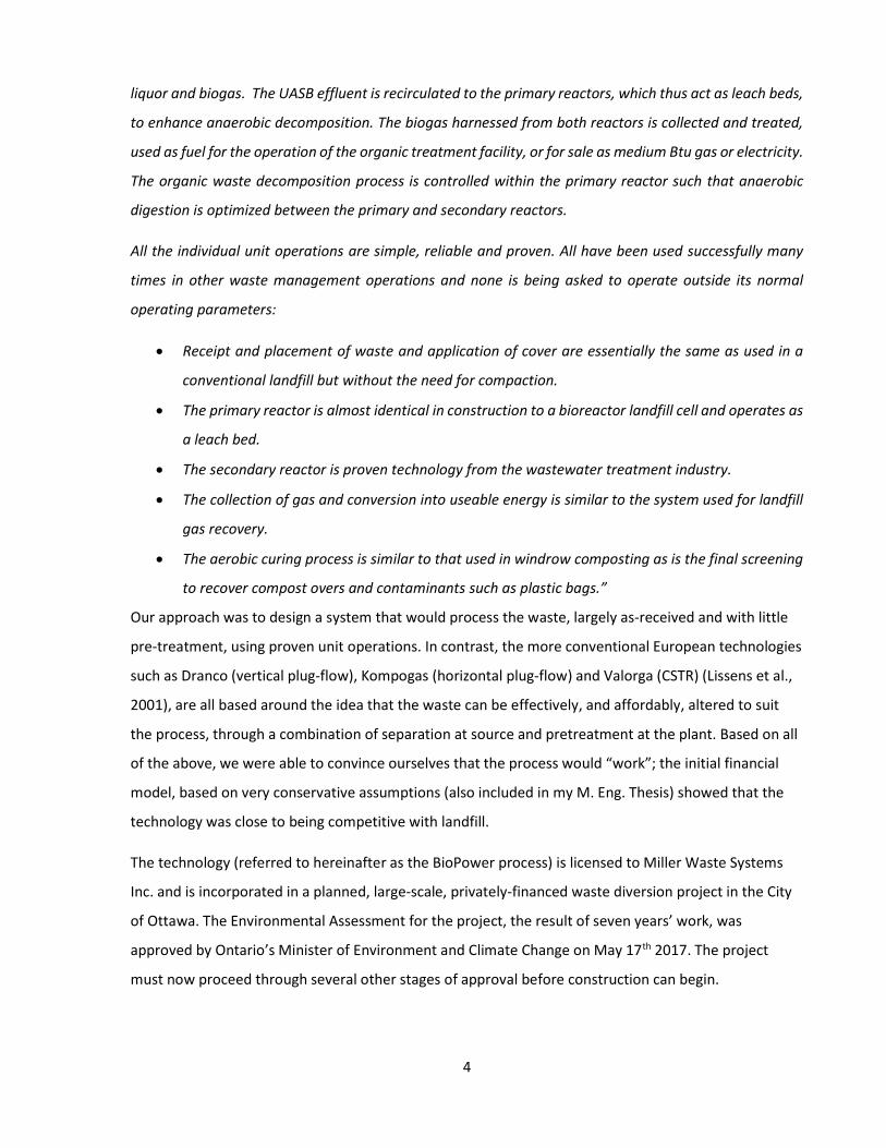
liquor and biogas. The UASB effluent is recirculated to the primary reactors, which thus act as leach beds,
to enhance anaerobic decomposition. The biogas harnessed from both reactors is collected and treated,
used as fuel for the operation of the organic treatment facility, or for sale as medium Btu gas or electricity.
The organic waste decomposition process is controlled within the primary reactor such that anaerobic
digestion is optimized between the primary and secondary reactors.
All the individual unit operations are simple, reliable and proven. All have been used successfully many
times in other waste management operations and none is being asked to operate outside its normal
operating parameters:
Receipt and placement of waste and application of cover are essentially the same as used in a
conventional landfill but without the need for compaction.
The primary reactor is almost identical in construction to a bioreactor landfill cell and operates as
a leach bed.
The secondary reactor is proven technology from the wastewater treatment industry.
The collection of gas and conversion into useable energy is similar to the system used for landfill
gas recovery.
The aerobic curing process is similar to that used in windrow composting as is the final screening
to recover compost overs and contaminants such as plastic bags.”
Our approach was to design a system that would process the waste, largely as-received and with little
pre-treatment, using proven unit operations. In contrast, the more conventional European technologies
such as Dranco (vertical plug-flow), Kompogas (horizontal plug-flow) and Valorga (CSTR) (Lissens et al.,
2001), are all based around the idea that the waste can be effectively, and affordably, altered to suit
the process, through a combination of separation at source and pretreatment at the plant. Based on all
of the above, we were able to convince ourselves that the process would “work”; the initial financial
model, based on very conservative assumptions (also included in my M. Eng. Thesis) showed that the
technology was close to being competitive with landfill.
The technology (referred to hereinafter as the BioPower process) is licensed to Miller Waste Systems
Inc. and is incorporated in a planned, large-scale, privately-financed waste diversion project in the City
of Ottawa. The Environmental Assessment for the project, the result of seven years’ work, was
approved by Ontario’s Minister of Environment and Climate Change on May 17th 2017. The project
must now proceed through several other stages of approval before construction can begin.
5
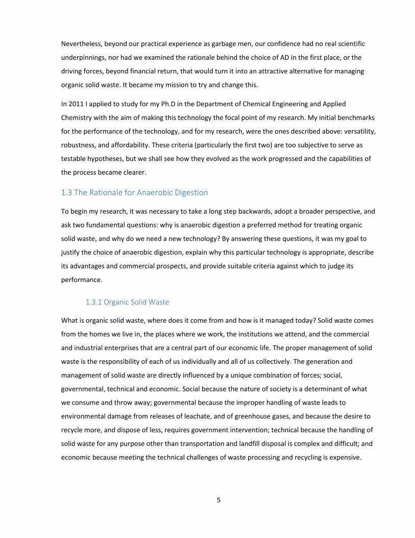
Nevertheless, beyond our practical experience as garbage men, our confidence had no real scientific
underpinnings, nor had we examined the rationale behind the choice of AD in the first place, or the
driving forces, beyond financial return, that would turn it into an attractive alternative for managing
organic solid waste. It became my mission to try and change this.
In 2011 I applied to study for my Ph.D in the Department of Chemical Engineering and Applied
Chemistry with the aim of making this technology the focal point of my research. My initial benchmarks
for the performance of the technology, and for my research, were the ones described above: versatility,
robustness, and affordability. These criteria (particularly the first two) are too subjective to serve as
testable hypotheses, but we shall see how they evolved as the work progressed and the capabilities of
the process became clearer.
1.3 The Rationale for Anaerobic Digestion
To begin my research, it was necessary to take a long step backwards, adopt a broader perspective, and
ask two fundamental questions: why is anaerobic digestion a preferred method for treating organic
solid waste, and why do we need a new technology? By answering these questions, it was my goal to
justify the choice of anaerobic digestion, explain why this particular technology is appropriate, describe
its advantages and commercial prospects, and provide suitable criteria against which to judge its
performance.
1.3.1 Organic Solid Waste
What is organic solid waste, where does it come from and how is it managed today? Solid waste comes
from the homes we live in, the places where we work, the institutions we attend, and the commercial
and industrial enterprises that are a central part of our economic life. The proper management of solid
waste is the responsibility of each of us individually and all of us collectively. The generation and
management of solid waste are directly influenced by a unique combination of forces; social,
governmental, technical and economic. Social because the nature of society is a determinant of what
we consume and throw away; governmental because the improper handling of waste leads to
environmental damage from releases of leachate, and of greenhouse gases, and because the desire to
recycle more, and dispose of less, requires government intervention; technical because the handling of
solid waste for any purpose other than transportation and landfill disposal is complex and difficult; and
economic because meeting the technical challenges of waste processing and recycling is expensive.
6
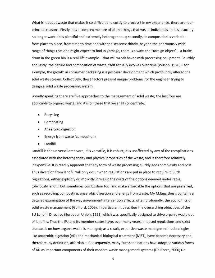
What is it about waste that makes it so difficult and costly to process? In my experience, there are four
principal reasons. Firstly, it is a complex mixture of all the things that we, as individuals and as a society,
no longer want - it is plentiful and extremely heterogeneous; secondly, its composition is variable -
from place to place, from time to time and with the seasons; thirdly, beyond the enormously wide
range of things that one might expect to find in garbage, there is always the “foreign object” – a brake
drum in the green bin is a real-life example – that will wreak havoc with processing equipment. Fourthly
and lastly, the nature and composition of waste itself actually evolves over time (Wilson, 1976) – for
example, the growth in consumer packaging is a post-war development which profoundly altered the
solid waste stream. Collectively, these factors present unique problems for the engineer trying to
design a solid waste processing system.
Broadly speaking there are five approaches to the management of solid waste; the last four are
applicable to organic waste, and it is on these that we shall concentrate:
Recycling
Composting
Anaerobic digestion
Energy from waste (combustion)
Landfill
Landfill is the universal omnivore; it is versatile, it is robust, it is unaffected by any of the complications
associated with the heterogeneity and physical properties of the waste, and is therefore relatively
inexpensive. It is readily apparent that any form of waste processing quickly adds complexity and cost.
Thus diversion from landfill will only occur when regulations are put in place to require it. Such
regulations, either explicitly or implicitly, drive up the costs of the options deemed undesirable
(obviously landfill but sometimes combustion too) and make affordable the options that are preferred,
such as recycling, composting, anaerobic digestion and energy from waste. My M.Eng. thesis contains a
detailed examination of the way government intervention affects, often profoundly, the economics of
solid waste management (Guilford, 2009). In particular, it describes the overarching objectives of the
EU Landfill Directive (European Union, 1999) which was specifically designed to drive organic waste out
of landfills. Thus the EU and its member states have, over many years, imposed regulations and strict
standards on how organic waste is managed; as a result, expensive waste management technologies,
like anaerobic digestion (AD) and mechanical biological treatment (MBT), have become necessary and
therefore, by definition, affordable. Consequently, many European nations have adopted various forms
of AD as important components of their modern waste management systems (De Baere, 2000; De

7
Baere, 2008; De Baere L., 2013). By comparison with the European Union, the regulations that have
governed organic waste diversion in North America in general, and the Province of Ontario in particular,
are less effective, which explains why advanced organic waste processing, particularly anaerobic
digestion, is very common in Europe and very rare in North America. This may finally be about to
change in Ontario with the enactment of the Waste Diversion Transition Act (Ontario, 2016), but no
regulations under the act have yet been promulgated, so the future remains uncertain.
How big is the problem? In Canada we still dispose of 25,000,000 tonnes of solid waste per year (after
recycling), all but a very small amount of it going to landfill. In Ontario about 76% of the solid waste
produced (before recycling) still goes to landfill (and most Provinces have similar records) (Canada,
2015; Government of Canada, 2010). Landfills generate leachate to be treated and biogas to be
collected (or released into the environment). Organic waste, as much as 40% of the total going to
landfill (Government of Ontario, 2004), is the principal source of this leachate and biogas, and its
diversion from disposal would meet the dual objectives of environmental protection and renewable
energy generation, defined as the production of energy from renewable resources that can replenish
themselves as rapidly as they are consumed, in this example the resource is biomass.
To define the nature and scope of the task in more precise terms, it is necessary to go beyond the big
picture just provided, and define the nature and sources of solid waste in general, and the organic solid
waste component in particular. Waste management terminology is inexact and varies significantly from
one political jurisdiction to another. In North America we define the sources of solid waste as:
MSW - municipal solid waste (originating from residences, both single family homes
and apartments)
IC&I - industrial, commercial and institutional waste
C&D construction and demolition waste
Such definitions are useful for large-scale planning purposes but not for designing waste processing
systems. Organic waste is present in the first two but not the third, which mostly consists of roof
shingles, brick, concrete and wood, with minor amounts of cardboard from the construction
component. The composition of residential solid waste, presented in Figure 1.2, comes from a study by
Mohareb (2008) and was obtained by hand-sorting garbage into separate piles and weighing each pile.
The composition of commercial and industrial waste comes from a report published by the City of
Ottawa (City of Ottawa, 2007) and is presented in Figure 1.3.
8
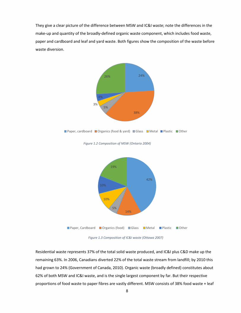
They give a clear picture of the difference between MSW and IC&I waste; note the differences in the
make-up and quantity of the broadly-defined organic waste component, which includes food waste,
paper and cardboard and leaf and yard waste. Both figures show the composition of the waste before
waste diversion.
Residential waste represents 37% of the total solid waste produced, and IC&I plus C&D make up the
remaining 63%. In 2006, Canadians diverted 22% of the total waste stream from landfill; by 2010 this
had grown to 24% (Government of Canada, 2010). Organic waste (broadly defined) constitutes about
62% of both MSW and IC&I waste, and is the single largest component by far. But their respective
proportions of food waste to paper fibres are vastly different. MSW consists of 38% food waste + leaf
24%
38%5%
3%
4%
26%
Paper, cardboard Organics (food & yard) Glass Metal Plastic Other
Figure 1.2 Composition of MSW (Ontario 2004)
42%
14%5%
10%
10%
19%
Paper, Cardboard Organics (food) Glass Metal Plastic Other
Figure 1.3 Composition of IC&I waste (Ottawa 2007)

9
and yard waste, plus 24% paper and cardboard, while IC&I waste consists of 14% food waste plus 47%
paper and cardboard. These figures serve as a guideline only, and should not be taken too literally for
planning purposes. They are subject to variability caused by methodology, which is anything but
standardized, the local balance of single-family/multifamily residences, the nature of local industry and
commerce, and the season of the year in which the samples were taken.
Some paper and cardboard can be, and is, recycled. Though more can be done, much of it is too
contaminated to be recovered economically, and therefore requires treatment as organic waste. In
many cities in Canada, food waste from single-family homes is separately collected and mostly
composted, but separate collection of food waste from multi-family homes (apartment buildings) is
very rare; it must therefore be disposed of without processing. Likewise, very little of the organic waste
from commercial and industrial sources is recovered, largely for reasons of cost; landfill is cheaper. It is
hard to estimate precisely how much organic waste, from all sources is being landfilled, but a Canada-
wide figure of 8,000,000 tonnes per year is probably conservative. This has implications for government
policy, the development of processing technologies, the economics of organic waste processing and the
generation of renewable energy.
1.3.2 The Case for Anaerobic Digestion
Fugitive releases of landfill gas, containing approximately 50% CH4, are a major source of greenhouse
gas emissions; 20 million tonnes per year as CO2eq. (Canada, 2013). Organic waste can be buried,
burned, composted or digested; how do these alternatives compare from an environmental,
particularly greenhouse gas emissions, perspective? Combinations of these options have been
compared by several authors using a lifecycle analysis approach. Bernstad and Jansen (2011) compared
incineration, composting, and anaerobic digestion of household food waste and concluded that AD has
the lowest GHG emissions. A direct comparison of landfill gas to energy with anaerobic digestion (with
electricity production) by Sanscartier et al.(2012), showed that under all circumstances AD was
environmentally preferred, but required financial subsidies. More recently, Hodge et. al. (2016)
conducted a very thorough LCA analysis of the management of food waste from industrial, commercial
and institutional sources in the United States, and concluded that, from a GHG perspective, anaerobic
digestion combined with landfill was the leading alternative in terms of global warming potential
reduction. They also noted that regulations governing the management of organic waste were
beginning to emerge in individual states and cities in the US. So the argument that the diversion of
organic waste from landfill is highly desirable is very strong. But the question still remains, how can this
be done economically within the current North American regulatory and economic framework?

10
1.3.3 The Rationale for a New Technology
The traditional chemical engineering approach to process design is driven by four objectives;
maximizing throughput, reducing hydraulic and solids retention times, reducing capital and operating
costs, and minimizing space requirements. Without costly source separation or extensive pretreatment,
this approach to anaerobic digestion will fail, and it is because of this that the proposed design is
different. It is premised on the idea of accepting slower reaction rates, longer retention times (in the
weeks to months range) and larger physical size, in exchange for simplicity of design and operation and
a larger footprint, with lower capital and operating costs than for conventional CSTR or plug flow
digesters of similar capacity.
There is also another, more subtle, aspect to the design. An anaerobic digester fulfils three purposes; it
reduces waste volume, it generates renewable energy and it produces a stabilized digestate when
combined with aerobic curing, but these purposes are not perfectly congruent. There will be
circumstances, related for example to process design or to substrate composition, in which stabilization
takes precedence over energy production or vice versa. From a waste manager’s perspective, volume
reduction and stabilization of the waste will always take priority over maximizing energy recovery.
There are two reasons for this; firstly, volume reduction and waste stabilization are the primary
objectives but, more importantly, it is also how most of the revenue is generated. The financial analysis
included in my M.Eng. thesis (Guilford, 2009) showed that only 30% of the gross revenue would be
generated from the sale of the recovered energy and 10% from the sale of compost, with 60% coming
from the tipping fee. It would take a profound increase in the value of renewable energy, or the
introduction of new regulations and incentives, to alter this circumstance because tipping fees are
market-specific, commercially competitive, and highly dependent on transportation cost. For these
reasons the engineering approach to this project is driven by the requirement to stabilize as much
organic waste as possible, and not by the desire to generate as much energy as possible, so whenever a
conflict between these two objectives arises waste stabilization prevails.
The proposed approach using a series of sequentially batch-fed leach bed reactors linked to a UASB (a
form of solid-state anaerobic digestion or SS-AD) has been successfully demonstrated at a laboratory
scale digesting grass silage (Nizami & Murphy, 2011). I have found no published research on the use of
this method to digest heterogeneous mixed solid waste of variable composition, or attempts to study
changing waste composition as a process variable. This is the starting point for the design of the
research programme.

11
Chapter 2. Objectives of the Research Programme
2.1 Starting Principles
Successful application of this approach to digesting heterogeneous and variable feedstocks can be
hypothesized by applying a specific set of propositions;
a) The range of organic wastes reliably treatable by AD, at an affordable cost, can be greatly
expanded beyond those originating from single-family homes, to include waste from multi-
family buildings and commercial/industrial/institutional sources.
b) The primary objective is to stabilize organic waste for environmental reasons, and the
secondary objective is to recover renewable energy for sale.
c) A reasonable proxy for the organic fraction of IC&I solid waste would comprise a mixture of
food waste, corrugated cardboard, boxboard, newsprint and fine paper, plus leaf and yard
waste.
d) The feedstock will receive as little pretreatment as possible.
e) By keeping the feedstock stationary and recirculating the liquids, the costs associated with
materials handling and pretreatment, and with equipment failure caused by the presence of
unwanted objects, can be dramatically reduced.
f) Compared to conventional AD (e.g. completely stirred tank and plug flow reactors) the mixing
of liquids and solids will be relatively inefficient; the reaction rate will be slower; the solids
retention time will be greater, the reactor volume larger, and more space will be required for a
plant of given throughput.
g) This trade-off will be economically advantageous.
h) Long-term process stability can be achieved by using multiple leach beds (charged with a blend
of organic waste and bulking agent, prepared with the minimum of pre-processing), with each
leach bed managed independently according to the properties of its contents and stage in the
digestion process, and all connected to a single UASB.
i) The composition of the waste can differ from one leach bed to another without causing process
instability.
j) Given the right biochemical and microbiological conditions, organic waste will digest, even if it
is heterogeneous and variable, and even if it contains foreign objects and undigestible waste
(below concentrations toxic to the process).
k) As the microbial community is converting the substrate, the community itself is evolving,
making it more, or less, resilient to sudden changes in the make-up of the substrate or the

12
presence of inhibitors; the effects of changes in the substrate under these circumstances are
not fully understood. By gaining an understanding the factors that enhance resilience and why,
it may be possible to maintain process stability when substrate changes occur.
l) Renewable energy in the form of biogas can be generated in commercial quantities.
m) The digested contents of each leach bed will require aerobic treatment (composting) as a final
step. The composted digestate may be too contaminated to be suitable for land application
which, while desirable, is less important than removing organics from landfill and generating
renewable energy.
Collectively, these propositions are different from those used as the basis of traditional AD and form
the starting point for setting out the objectives and planning the PhD research programme. The specific
objectives which follow are influenced, in part, by the Literature Review presented in Chapter 4.
2.2 Specific Objectives
1) Design, build, and commission a laboratory scale version of the BioPower process
2) Test and troubleshoot the initial operation to confirm operability and create a baseline for
subsequent experiments
3) Develop analytical methodology and a sampling plan compatible with the operation of the
digester that will enable mass and energy balance calculations and performance monitoring
and benchmarking to other systems
4) Operate the reactor under a variety of test conditions to measure efficiency in terms of biogas
yield, COD destruction and solids stabilization, as well as robustness and stability, starting with
examining the effects of changes in substrate composition
5) Use the performance data obtained to refine economic predictions for a full scale system
2.3 Hypothesis
The hypothesis that the research programme has been designed to test is as follows:
An anaerobic digester, comprising multiple sequentially-fed leach beds feeding a single UASB is capable of successfully processing mixed organic wastes, consisting of varying proportions of cellulosic wastes (paper, cardboard, boxboard) and food waste, to produce commercial quantities of biogas and a stabilized digestate.
This can be accomplished by managing the leach beds independently of one another, balancing leachate flow between recirculation to the leach beds and delivery to the UASB, allowing adequate solids retention time to achieve the maximum practical conversion of biomass to biogas, and by aerobically curing the digestate. Digestion rate and yield can be enhanced by managing the proportion of food waste to fibres; the production of waste water (except for water-of-saturation in the digestate) can be

13
minimized or even eliminated; process stability can be maintained, despite feedstock variability, by controlling two principal variables; C:N ratio and alkalinity.

14
Chapter 3. Thesis Outline
The body of the thesis is laid out as follows. The literature review is presented in Chapter 4 and
concludes with a summary and a statement of the knowledge gaps. Chapter 5 describes the process of
system design through to the completion of the construction of the lab scale digester. A description of
the analytical methods follows in Chapter 6. Commissioning and startup are covered in Chapter 7;
startup is divided into three segments and concludes with 10 weeks of stable operation, creating a
baseline for the experiments that follow. Chapter 8 is a description of digester operations through 83
weeks, divided into six operating periods each devoted to a particular aspect of the research, for
example changes in feedstock composition. To complement the data obtained from the operation of
the digester, three supporting experiments were conducted, related to substrate digestibility and
aerobic curing; these are described in Chapter 9. Results, discussion, conclusions and recommendations
are presented in Chapter 10. The appendices are in two parts; additional information in the form of
figures and tables, plus large data files in electronic form to be made available through TSpace at:
https://tspace.library.utoronto.ca/handle/1807/9945
15
Chapter 4. Literature Review
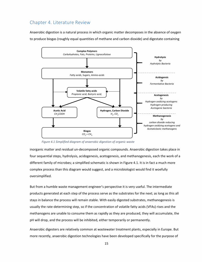
Anaerobic digestion is a natural process in which organic matter decomposes in the absence of oxygen
to produce biogas (roughly equal quantities of methane and carbon dioxide) and digestate containing
inorganic matter and residual un-decomposed organic compounds. Anaerobic digestion takes place in
four sequential steps, hydrolysis, acidogenesis, acetogenesis, and methanogenesis, each the work of a
different family of microbes; a simplified schematic is shown in Figure 4.1. It is in fact a much more
complex process than this diagram would suggest, and a microbiologist would find it woefully
oversimplified.
But from a humble waste management engineer’s perspective it is very useful. The intermediate
products generated at each step of the process serve as the substrates for the next; as long as this all
stays in balance the process will remain stable. With easily digested substrates, methanogenesis is
usually the rate-determining step, so if the concentration of volatile fatty acids (VFAs) rises and the
methanogens are unable to consume them as rapidly as they are produced, they will accumulate, the
pH will drop, and the process will be inhibited, either temporarily or permanently.
Anaerobic digesters are relatively common at wastewater treatment plants, especially in Europe. But
more recently, anaerobic digestion technologies have been developed specifically for the purpose of
Hydrolysis by
Hydrolytic Bacteria
Complex Polymers Carbohydrates, Fats, Proteins, Lignocellulose
Monomers Fatty acids, Sugars, Amino-acids
Hydrogen, Carbon Dioxide H2, CO2
Volatile fatty acids Propionic acid, Butryric acid,
Biogas CO2 + CH4
Acetic Acid CH3COOH
Acidogensis by
Fermentative Bacteria
Methanogenesis by
carbon dioxide reducing hydrogen oxidizing acetogens and
Acetaticlastic methanogens
Acetogenesis by
Hydrogen oxidizing acetogens Hydrogen-producing Acetogenic bacteria
Figure 4.1 Simplified diagram of anaerobic digestion of organic waste

16
treating organic solid waste. This occured in response to environmental regulations, particularly in
Europe, requiring the diversion of organic wastes from landfill. Regulations provide an economic driving
force for technical development in the field, a subject that I studied for my M.Eng. (Guilford, 2009).
The application of anaerobic digestion to organic solid waste brings with it greater complexities and
engineering challenges than does the treatment of wastewaters streams. The research performed on
the anaerobic digestion of solid waste is the subject of this literature review, which focuses on the solid
state anaerobic digestion (SS-AD) of food waste, cardboard, boxboard (e.g. cereal boxes), newsprint,
fine paper and wood chips.
4.1 What Kind of Anaerobic Digester?
To choose a basic design concept for an anaerobic digester intended for the treatment of solid waste,
three binary decisions have to be made;
o “wet” or “dry” (an operational distinction, generally taken to mean below 12% or above 20% total solids),
o single-stage or two-stage, and
o mesophilic (37°C) or thermophilic (55°C).
Nizami & Murphy (2010) reviewed the pros and cons of “wet” versus “dry”. The “wet” process operates
from 2-12% solids; the “dry” process operates from 20 - 50% solids. The dry process requires simpler
pretreatment and consumes less energy, but mixing of substrates and materials handling are more
complex. The wet process despite a longer operating history (from wastewater treatment) has
shortcomings; high water consumption and sensitivity to shock-loadings among them. In many respects
this choice must be made based upon the properties of the substrates.
A single-stage digester is obviously less complex and less expensive to build, but the two-stage
alternative has, at least in theory, certain advantages. In particular by operating the first stage at lower
pH, substrate hydrolysis can be enhanced; the two-stage process is also said to be more robust and less
susceptible to failure (Nizami et al., 2010). The theory behind two-stage digestion is a simple one;
hydrolysis of the solid substrate and acidogenesis take place in the first stage, then the leachate
containing VFAs and other soluble intermediate products is fed to a methanogenic reactor where they
undergo acetogenesis and methanogenesis by a consortium of archaea and bacteria, see Figure 4.1. In
practice it is not so clear-cut; biogas can be generated in the first reactor and in the leachate storage
tanks, as well as the methanogenic reactor; also the role and behaviour of the first reactor can change
with the age of waste that it contains. Nevertheless, two-stage digestion of many substrates, including

17
organic solid waste, has been shown to have important advantages over single-stage systems, for
example minimal feedstock preparation and digester stability. The literature shows that the single-
stage digester of choice is generally a CSTR, and that two-stage digesters comprise either a leach bed or
a CSTR coupled to a methanogenic reactor, commonly a UASB but sometimes an anaerobic filter (Mata-
Alvarez et al., 2000). Some work has been performed using two CSTRs in series; in one example Banks
et al. (1998) used a two-stage CSTR, digesting a mixture of lignocellulosic wastes, to demonstrate
enhanced process stability, when compared to a single CSTR, by flushing VFAs from the first reactor to
the second. Also, two CSTRs operating in series, digesting highly degradable food waste, showed
enhanced process stability (Pavan et al., 2000). Chugh et al. (1999) tested a pair of leach beds operating
in series, digesting MSW; the system was set up with fresh waste in the first leach bed and stabilized
waste in the second. The result was accelerated substrate degradation compared to a single-stage LB
under similar conditions.
In a 20 day side-by-side comparison of a single leach bed alone with a leach bed coupled to a UASB,
digesting presorted MSW, the two-stage digester gave a 30% greater methane yield and 2.5x the
volatile solids reduction (O'Keefe & Chynoweth, 2000). In a side-by-side comparison of a single-stage
CSTR to a two-stage reactor comprising 6 Leach beds and a UASB digesting grass silage, Nizami &
Murphy (2010) showed that, while the CSTR gave higher yields (451 L CH4 kg-1VSadded in 50d vs. 341 L
CH4 kg-1VSadded in 30d, the two-stage reactor could operate at higher loading rates, was more versatile,
and purported to be less expensive at commercial scale. In a very recent paper, Di Maria (2017)
obtained similar results from single-stage digestion of OFMSW; a CSTR gave yields of 320
L.CH4.kg-1VSadded, compared to a LB which gave 250 L CH4 kg-1VSadded; they also confirmed the benefits of
leachate recirculation to improve the digestion efficiency of SS-AD. Siegert & Banks (2005) showed that
the separation of the process into two stages makes it possible to minimize VFA accumulation and
prevent acidification from inhibiting hydrolysis in the leach bed first stage, while maintaining a higher
pH in the UASB second stage. Nizami and Murphy (2011a), using grass silage as substrate, maintained a
pH 5.9 in the leach beds and pH 7.4 in the UASB, creating favourable conditions for hydrolysis and
acidogenesis in stage 1 followed by acetogenesis and methanogenesis in stage 2.
A side-by-side comparison of mesophilic and thermophilic digestion of cardboard and paper, in a 150
day experiment by Qu et al. (2009), showed that higher methane yields were generated in the
mesophilic system. For the digestion of food waste, mesophilic digestion was shown to be more stable
than thermophilic (Yirong C., 2013). Mata-Alvarez et al.(2000) in their review paper, found that the
benefits of thermophilic digestion depended on the substrate, and that sometimes these were offset by
18
higher energy demands. Kim (2012) compared the hydrolysis of organic wastes under thermophilic and
mesophilic conditions in sequencing batch reactors, finding that protein hydrolysis at thermophilic
temperatures was four times faster than at mesophilic.
De Baere (2000) reported on the prevalence of various commercial reactor designs across Europe with
the following results; Europe is 38% “wet” and 62% “dry”; 93% single stage and 7% two stage; 67%
mesophilic and 33% thermophilic. The dominance of single stage digestion is presumably because,
when the feedstock has been extensively pre-treated, two-stage no longer offers sufficient advantages
to justify the cost.
Summary (Digester design concept) Both wet and dry anaerobic digestion technologies are proven, both in the laboratory and on a
commercial scale. The choice of which to use is largely dependent on the physical properties of the substrates, and the amount of pretreatment given to the waste.
A lot of laboratory research has been devoted to two-stage versus single-stage anaerobic digestion, partly because two-stage digestion appears to offer advantages for solid substrates. However, single-stage digestion is by far the more common in commercial applications, for reasons of economics and simplicity.
Far less research has been conducted on direct comparisons of mesophilic and thermophilic digestion and the results are somewhat inconclusive. Nevertheless, both work successfully at a commercial scale. Thermophilic is also a greater challenge in cold climates but does a better job of killing pathogens, a necessary step that can also be accomplished during aerobic curing to create a compost product.
4.2 Substrates, Bulking Agent and Digestate
As we have seen, organic solid waste from municipal and commercial sources consists primarily of food
waste and various lignocellulosic fibres such as cardboard, boxboard, newspaper etc., plus leaf and yard
waste. From the perspective of their behaviour in the AD process and their biodegradability, substrates
can be divided into two separate groups; firstly FW alone, secondly wood-derived fibres collectively
(FB) and unprocessed wood, the bulking agent (BA).
Food waste is one of the most extensively studied substrates for anaerobic digestion; it is produced in
large quantities and, improperly managed, it presents an environmental threat; but it is a readily-
digestible source of renewable energy. Lignocellulosic wastes are produced in even larger quantities,
with much greater renewable energy potential (per dry tonne), but they digest more slowly and,
arguably, are less of an environmental threat as a result. This section reviews the relationship between
the digestion process and the substrates and their properties under the following headings:
o Food Waste o Lignocellulosic waste

19
o Co-digestion o Feedstock preparation o Size reduction o Digester solids content o Bulking agent in anaerobic digestion o Digester performance – predictions from the literature o Aerobic curing – the final step
4.2.1 Food Waste
Food waste contains many things, fruits and vegetables, meats, dairy products, baked goods, peelings
and trimmings from fresh waste, plate scrapings, bones, shells, paper towels and much more besides.
Furthermore, composition depends on the season of the year, methods of collection, the socio-
economic circumstances of the people generating it, and subsequent preprocessing. Five descriptive
terms are common in the literature (Guilford, 2009; Zhang et al., 2008);
Source separated organic fraction of municipal solid waste (ss-OFMSW) Mechanically recovered organic fraction of municipal solid waste (mr-OFMSW) Fruit and vegetable waste (FVW) Canteen or cafeteria waste (a more restricted, less contaminated, version of ss-OFMSW) Source-separated organics (SSO)
This last term is a North American version of ss-OFMSW. These are all operating definitions of
convenience and cannot be relied upon for anything beyond general guidance. There are probably as
many definitions of food waste (or indeed any other organic waste) as there are laboratories studying
it, and this makes inter-laboratory comparison of research very difficult. Often, but not always, the
situation is made clearer by the inclusion of an analysis of the food waste.
The example shown in Table 4.1 is a very detailed comparison of the properties of ss-OFMSW and ms-
OFMSW from Zhang et al. (2012a); it illustrates how different source-separated and mechanically-
separated waste streams can be. Zhang used the data to estimate the biochemical methane potential
(BMP) of the two waste samples using three different methods, biochemical composition, the Buswell
equation, and a carbon mass balance. The biochemical composition was derived from the work of
Angelidaki & Ellegaard (2003), who calculated the theoretical methane yields of several substrates. It
appears that Zhang et al. (2012a) appropriated these data by assuming that lignocellulosic products
could be treated as carbohydrates, though this is not explained in their work.
The Buswell equation method (Banks et al., 2012; Nizami et al., 2011) is based on elemental analysis
and stoichiometry; the result is the maximum possible yield of methane, assuming 100% chemical

20
oxygen demand (COD) conversion. The carbon mass balance was based on the measured destruction of
volatile solids (VS) and biogas composition, which explains why it is closest to the measured values.
Table 4.1 Comparison of the Properties of ss-FW and mr-OFMSW
ss-MSW mr-OFMSW
General
Total solids (TS) 24 53
Volatile solids (VS) (% of TS) 91 64
Biochemical composition (g/kg) (VS basis)
Carbohydrates 453 340
Lipids 151 69
Crude proteins 235 130
Hemicellulose 38 52
Cellulose 50 252
Lignin 17 184
Nutrients and potentially toxic elements (TS basis)
TKN (g.kg-1) 34.2 13.9
Total phosphorus (g.kg-1) 5.41 2.17
Total potassium (g.kg-1) 14.3 4.26
Cd (mg.kg-1) <1.0 1.50
Cr (mg.kg-1) 29.0 263
Cu (mg.kg-1) 7.2 107
Hg (mg.kg-1) <0.010 0.179
Ni (mg.kg-1) 7.0 97.0
Pb (mg.kg-1) <10 162
Zn (mg.kg-1) 33 259
Elemental composition) (TS basis) (TS basis) (VS basis)
C (%) 47.6 33.0 53.6
H (%) 7.0 4.8 7.80
O (%) 33.3 22.2 36.1
N (%) 3.4 1.3 2.14
S (%) 0.15 0.25 0.41 Adapted from (Zhang et al., 2012a)
The two substrates were digested in CSTRs, in a side-by-side experiment, which ran for 284 days. The
BMP data are compared to the experimental digester performance data in Table 4.2. These results
illustrate three important points, the marked difference in waste properties and digester behaviour
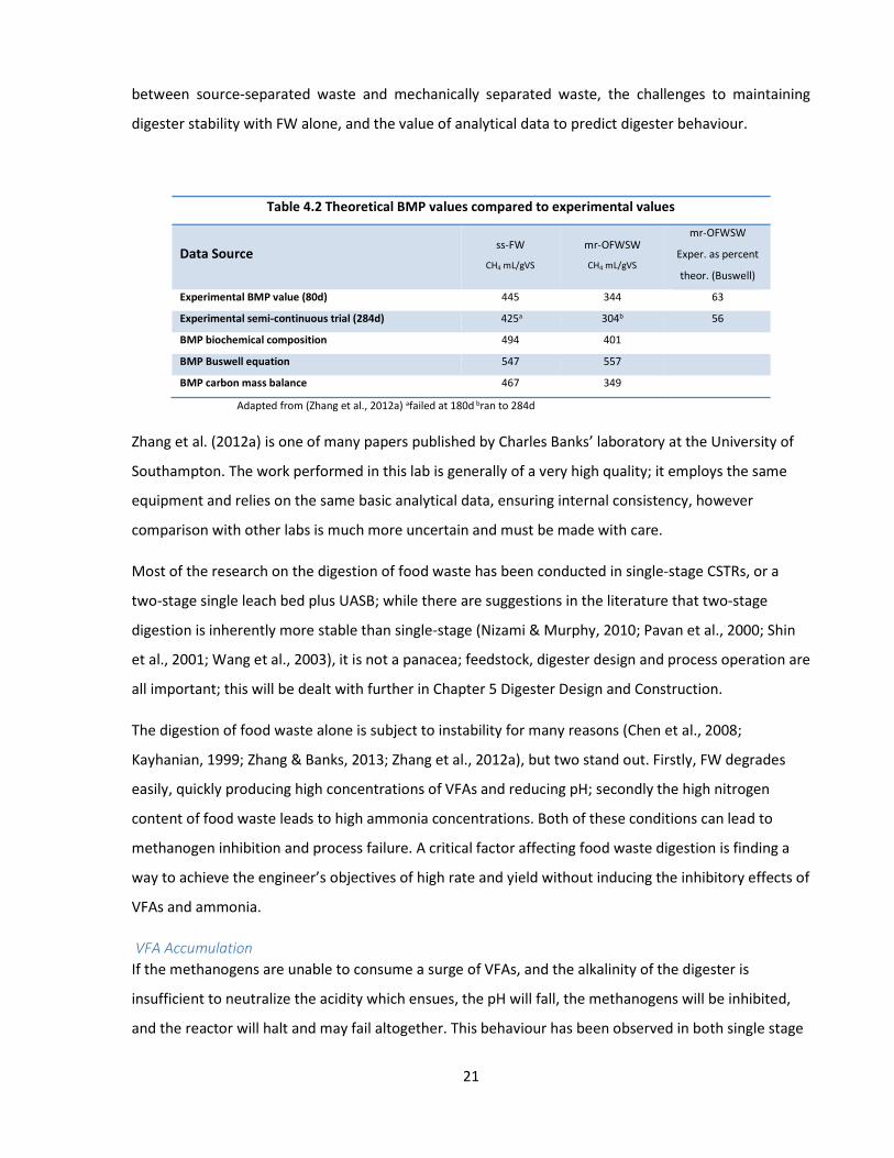
21
between source-separated waste and mechanically separated waste, the challenges to maintaining
digester stability with FW alone, and the value of analytical data to predict digester behaviour.
Table 4.2 Theoretical BMP values compared to experimental values
Data Source ss-FW
CH4 mL/gVS
mr-OFWSW
CH4 mL/gVS
mr-OFWSW
Exper. as percent
theor. (Buswell)
Experimental BMP value (80d) 445 344 63
Experimental semi-continuous trial (284d) 425a 304b 56
BMP biochemical composition 494 401
BMP Buswell equation 547 557
BMP carbon mass balance 467 349
Adapted from (Zhang et al., 2012a) afailed at 180d bran to 284d
Zhang et al. (2012a) is one of many papers published by Charles Banks’ laboratory at the University of
Southampton. The work performed in this lab is generally of a very high quality; it employs the same
equipment and relies on the same basic analytical data, ensuring internal consistency, however
comparison with other labs is much more uncertain and must be made with care.
Most of the research on the digestion of food waste has been conducted in single-stage CSTRs, or a
two-stage single leach bed plus UASB; while there are suggestions in the literature that two-stage
digestion is inherently more stable than single-stage (Nizami & Murphy, 2010; Pavan et al., 2000; Shin
et al., 2001; Wang et al., 2003), it is not a panacea; feedstock, digester design and process operation are
all important; this will be dealt with further in Chapter 5 Digester Design and Construction.
The digestion of food waste alone is subject to instability for many reasons (Chen et al., 2008;
Kayhanian, 1999; Zhang & Banks, 2013; Zhang et al., 2012a), but two stand out. Firstly, FW degrades
easily, quickly producing high concentrations of VFAs and reducing pH; secondly the high nitrogen
content of food waste leads to high ammonia concentrations. Both of these conditions can lead to
methanogen inhibition and process failure. A critical factor affecting food waste digestion is finding a
way to achieve the engineer’s objectives of high rate and yield without inducing the inhibitory effects of
VFAs and ammonia.
VFA Accumulation If the methanogens are unable to consume a surge of VFAs, and the alkalinity of the digester is
insufficient to neutralize the acidity which ensues, the pH will fall, the methanogens will be inhibited,
and the reactor will halt and may fail altogether. This behaviour has been observed in both single stage

22
CSTRs (Zhang et al., 2012a), and two-stage digesters employing leach beds and a USAB (Browne, 2013;
Browne et al., 2013); it can occur at any time in a long-running experiment, sometimes prompted by
operational changes (Climenhaga & Banks, 2008a; Climenhaga & Banks, 2008b) but sometimes for no
apparent reason (Jiang et al., 2012; Zhang & Banks, 2013; Zhang et al., 2012a). The wash-out of crucial
trace elements, particularly Se, Co and W, which are specifically required by certain enzymes for
methanogenesis, is one contributing cause. Comparing reactors with and without trace element
supplements showed that the former remain stable much longer – 520d vs. 120d. (Banks et al., 2012;
Jiang et al., 2012). In a parallel study, Zhang et al. (2012b) maintained stability by adding a mixture of
CB and BB to the food waste, instead of adding trace elements; as a result a reactor facing incipient
failure was restored to stability, though this did not happen immediately, taking about 90 days in all. It
has also been shown that lengthening the hydraulic retention time (HRT) to reduce loss of trace
elements by wash-out can prevent, or greatly postpone, reactor failure (Climenhaga & Banks, 2008a;
Nagao et al., 2012). Conversely, and somewhat paradoxically, three articles show that flushing
accumulated VFAs out of a leach bed reactor to a UASB in a two-stage digester, stabilizes digester
operation (Climenhaga & Banks, 2008b; Han & Shin, 2004; Shin et al., 2001); note that the SRT of these
experiments was between 25 and 30 days. There is another perspective; Stroot et al. (2001) conducted
an extensive study of the single-stage anaerobic digestion of a synthetic OFMSW under mesophilic
conditions, operated semi-continuously with daily wasting and feeding, using either cattle manure or
waste activated sludge as inoculum. The variables studied were organic loading rates and mixing
practices. They determined that waste activated sludge was superior to cattle manure, that minimal
mixing led to higher yields than continuous mixing – especially at higher OLRs, and that unstable,
continuously mixed, reactors could be stabilized by shifting to minimal mixing. The continuously mixed
reactors consistently showed a propionate buildup. Two possible explanations for this behaviour were
proposed, physical disruption of the syntrophic relationship between hydrolytic/acidogenic bacteria
and methanogenic archaea, or overloading the methanogens with high concentrations of hydrolysis
and fermentation products, resulting from continuous mixing.
Inhibition of methanogens at a low pH is always preceded by a sharp rise in VFA concentration.
However, if the system is well buffered, the pH remains high and the VFAs are consumed. The best
indicator of impending reactor failure is the alkalinity ratio, used in one form or another by most of the
researchers cited in this section. It is a titrimetric method and there are several versions; the most
commonly used appears to be that of Ripley which, for reasons explained in Section 6.4, I adopted for
use in this study.

23
Ammonia Accumulation Food waste has a relatively high nitrogen content, which originates from leafy vegetables and the
proteins in meats and leads to a low C:N ratio. If the amount of nitrogen present in the digester is
greater than the metabolic requirements of the microbial community for sustenance and growth, the
excess will form ammonia which is inhibitory to methanogens, particularly in the undissociated NH3
form present at higher pH; Kayhanian (1999) reported inhibition at total ammonia concentrations of
1200mg.L-1 with a free NH3 concentration of 45 mg.L-1, at pH7.2. This condition generally occurs when
the C:N ratio is <15; for safety it should be >20 (Igoni et al., 2008; Wu et al., 2010; Yadvika, 2004). For
example, in a side-by-side experiment by Zhang et al. (2012a), mr-OFMSW with a C:N ratio of 25:1
remained stable, but SS-OFMSW with a C:N ratio of 14:1 failed. There are only three practical ways of
maintaining digester stability in this situation; ensuring that the C:N ratio is always high enough by
adding a carbon source, diluting the contents of the reactor with water if ammonia levels rise to
inhibitory concentrations (Kayhanian, 1999), and operating with a long SRT (Bhattacharya & Parkin,
1989; Chen et al., 2008). As we shall see later, the C:N ratio in my experiments never fell below 45:1
and was usually much higher; as a result the reactor never experienced ammonia inhibition.
Summary (Food waste) Food waste must be analyzed thoroughly and its properties defined well; definitions of
convenience cannot be relied upon. Rapid initial digestion and surges in VFA concentration must be expected along with the potential
for inhibition; this can be managed by allowing longer HRT and SRT and by including a high rate reactor.
pH and alkalinity are indicators of incipient instability or inhibition. Ammonia inhibition is a distinct possibility when digesting FW alone; stability is best achieved by
maintaining the C:N ratio above 20 to 1 and operating with a long SRT. Food waste digestibility will be between 60% and 80% depending on its make-up, the content of
inorganics, and proportion of lignocellulosic materials (see Section 4.4 for further discussion). A digester that is operable over a wide range of HRTs and SRT’s has greater operating flexibility. Mixing and stirring should be kept to a practical minimum.
4.2.2 Lignocellulosic Waste
Data on composition and properties of typical fibres are presented in summary tables derived from
several sources. Table 4.3 shows the elemental analysis for fine paper (FP), newsprint (NP) and
cardboard (CB); these are the data from several publications, abstracted from Zhou et al. (2016) and
averaged.

24
Table 4.4 shows a typical example of the physicochemical properties of the same three fibres. All of
these materials consist of a combination of cellulose, hemicellulose and lignin, not all of which is
convertible to biogas. Lignin itself is very
resistant to digestion, but it is also bound to the
cellulose and hemicellulose, protecting them
from attack by microbes and enzymes; as a
result, cellulose and hemicellulose hydrolyze
slowly. All of these lignocellulosic fibres are derived from wood pulp, and the pulping process has a
direct influence on their
biodegradability and the methane yield
which they generate. Newsprint (NP) is
made from mechanically ground wood
without the addition of chemicals to
remove lignin. Both cardboard (CB) and
boxboard (BB) are made from
unbleached Kraft paper. The Kraft
process involves chemical treatment to partially remove lignin. Fine paper (FP) is made from bleached
Kraft paper and has virtually no lignin. The biodegradability and methane yields of these materials,
obtained from three publications, are presented in Table 4.5. Although the data are incomplete, and
the absolute values for biodegradability and methane yield vary from one source to another, all show
the same descending order of biodegradability, FP > CB > NP; this ranking may be related to the pulping
process used in their manufacture, and their resultant biochemical makeup.
Abstracted from (Buffiere et al., 2008b; Eleazer et al., 1997; Owens & Chynoweth, 1993; Yuan et al., 2012; Yuan et al., 2014) ND - not determined
Pommier (2010) created a blend of lignocellulosic fibres, consisting of a mixture of office paper,
newspaper, corrugated carton, cardboard and magazine stock, to simulate MSW. The physical
Table 4.3 Elemental Composition of 3 Lignocellulosic Wastes
Substrates C H O N C:N Ratio
Fine paper 44.76 5.29 49.81 0.10 448
Newspaper 46.70 5.23 48.03 0.17 275
Cardboard 47.31 6.15 46.00 0.33 143
Abstracted from (Zhou et al., 2014)
Table 4.4 Physicochemical Properties of 3 Lignocellulosic Wastes
Parameter Fine Paper (FP) Newsprint (NP) Cardboard (CB)
TS (%) 95.3 93.2 95.4
VS (% TS) 98.6 96.1 87.2
Ash (% TS) 1.4 3.9 12.8
Lignin (% TS) 1.4 23.4 17.8
Cellulose (% TS) 84.9 68.5 56.9
Hemicellulose (% TS) 12.3 13.1 10.7
COD g/g TS 1.07 1.21 1.10
Adapted from Yuan et al. (2012)
4.5 Biodegradability and Methane Yield Data of 3 Lignocellulosic Substrates
Eleazer Owens and
Chynoweth
Buffiere Yuan
Substrates % VS
destr.
CH4
mL/gVS
% VS
destr.
CH4
mL/gVS
% VS
destr.
CH4
mL/gVS
% VS
destr.
CH4
mL/gVS
Fine paper (FP) 54.6 288 ND 369 67.9 351.4 ND 208
Cardboard (CB) 54.4 155 ND 278 50.1 239.8 ND 96
Newsprint (NP) 31.1 74 ND 100 ND ND ND 75
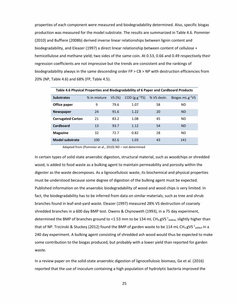
25
properties of each component were measured and biodegradability determined. Also, specific biogas
production was measured for the model substrate. The results are summarized in Table 4.6. Pommier
(2010) and Buffiere (2008b) derived inverse linear relationships between lignin content and
biodegradability, and Eleazer (1997) a direct linear relationship between content of cellulose +
hemicellulose and methane yield; two sides of the same coin. At 0.53, 0.66 and 0.49 respectively their
regression coefficients are not impressive but the trends are consistent and the rankings of
biodegradability always in the same descending order FP > CB > NP with destruction efficiencies from
20% (NP, Table 4.6) and 68% (FP, Table 4.5).
Table 4.6 Physical Properties and Biodegradability of 6 Paper and Cardboard Products
Substrates % In mixture VS (%) COD (g.g-1TS) % VS destr. Biogas mL.g-1VS
Office paper 9 79.6 1.07 58 ND
Newspaper 24 91.6 1.22 20 ND
Corrugated Carton 21 83.2 1.08 45 ND
Cardboard 13 93.7 1.12 54 ND
Magazine 32 72.7 0.82 28 ND
Model substrate 100 82.6 1.03 43 141
Adapted from (Pommier et al., 2010) ND – not determined
In certain types of solid state anaerobic digestion, structural material, such as woodchips or shredded
wood, is added to food waste as a bulking agent to maintain permeability and porosity within the
digester as the waste decomposes. As a lignocellulosic waste, its biochemical and physical properties
must be understood because some degree of digestion of the bulking agent must be expected.
Published information on the anaerobic biodegradability of wood and wood chips is very limited. In
fact, the biodegradability has to be inferred from data on similar materials, such as tree and shrub
branches found in leaf-and-yard waste. Eleazer (1997) measured 28% VS destruction of coarsely
shredded branches in a 600 day BMP test. Owens & Chynoweth (1993), in a 75 day experiment,
determined the BMP of branches ground to <1.53 mm to be 134 mL CH4.gVS-1added, slightly higher than
that of NP. Trzcinski & Stuckey (2012) found the BMP of garden waste to be 114 mL CH4.gVS-1added in a
240 day experiment. A bulking agent consisting of shredded ash wood would thus be expected to make
some contribution to the biogas produced, but probably with a lower yield than reported for garden
waste.
In a review paper on the solid-state anaerobic digestion of lignocellulosic biomass, Ge et al. (2016)
reported that the use of inoculum containing a high population of hydrolytic bacteria improved the

26
degradation of cellulosic and hemicellulosic substrates. Xu et al. (2013) identified dairy waste effluents
in particular as being the most beneficial in this respect.
Summary (Lignocellulosic wastes) Expect slow rates of digestion and low yields and, as a consequence, a long SRT. Neither VFAs nor ammonia are expected to be present in sufficient quantities to cause digester
instability. There is no published information on the properties of coated cardboard, referred to in North
America as boxboard, or its biodegradability. An educated guess would suggest that BB would behave similarly to CB but with lower yields because of the coatings.
Fibre biodegradability is ranked FP > CB > NP. Digestibility ranges from 30% to 70% depending on the fibre; the main determinant is lignin
content. Hydrolytic bacteria in the inoculum are beneficial for the hydrolysis of lignocellulosic wastes. The C:N ratio of any combination of fibres will be very high, but the addition of FW will lower
the ratio in proportion to the amount of food waste added. Substrates should be analyzed to permit calculation of BMPtheor. for both reactor design
purposes and performance measurement. 4.2.3 Co-digestion
Co-digestion is the combined digestion of two or more substrates for the purpose of improving digester
performance, defined in terms of yield, rate and stability. Depending upon the substrates chosen and
reactor conditions, co-digestion can improve all three. In a review paper, Mata-Alvarez et al. (2011)
highlight the two most active areas of co-digestion research, based on an analysis of the number of
publications in the literature; they are sewage sludge plus organic fraction of municipal solid waste
(OFMSW), followed by co-digestion in the agricultural sector – farm wastes and energy crops. Among
the citations are eighteen references to co-digestion of OFMSW and sewage sludge with other
substrates, only one of which, pulp and paper mill sludge, is a cellulosic material (Zhang et al., 2008). In
a more recent review paper, Esposito et al. (2012) cite numerous examples of substrate combinations
but, once again, only one involves co-digestion of OFMSW with cellulosic waste - in this case biosludge -
in a paper by PoggiVaraldo et al. (1997) and the reported results are of limited value to this study.
Thus the situation respecting the co-digestion of the two major components of MSW, food waste and
cellulosic fibres, is rather strange. Usually they are generated together, sometimes they are separated
prior to treatment or disposal, but more often they are collected and processed or disposed of
together. Yet research on their co-digestion is basically nonexistent. The only significant exceptions are
studies of anaerobic decomposition in simulated landfills (Eleazer et al., 1997; Ledakowicz & Kaczorek,
2004; Yazdani, 2010), but these are of limited help because the experiments were not designed to
27
assess the contributions of the individual co-substrates, or their respective influence on one another in
the digestion process. Finally, from a commercial perspective, co-digestion has achieved limited
success. De Baere (2013) reported that only 11% of installed anaerobic digestion capacity in Europe
employs some form of co-digestion, most of which is concentrated in the agri-industrial sector.
Summary (Co-digestion) Interest in the co-digestion of organic wastes has grown significantly in recent years, as
evidenced by the increase in the number of research publications. OFMSW and sewage sludge are two of the most popular substrates for co-digestion. Paper and cardboard and other wood-pulp-derived substrates have received little or no
attention in this respect. I can find no publications examining the co-digestion of FW and FB for any purpose other than
improving stability of FW digestion.
4.3 Feedstock Preparation
Given the physical properties of organic solid waste, some form of feedstock preparation is generally
required prior to anaerobic digestion. It can involve size reduction, water addition, the use of a bulking
agent, or a pretreatment step (or some combination of these) to improve the biodegradability of the
substrates. Each of these is discussed in what follows.
4.3.1 Size Reduction in SS-AD
There are three principal reasons for size-reducing feedstock in SS-AD; to improve biodegradability
(both rate and yield), to reduce channeling in leach bed reactors, and to improve uniformity for
analytical purposes. Chynoweth et al. (1993) measured the Biochemical Methane Potential (BMP) of
MSW which had been ground to various particle sizes, and found that the yield changed little, but that
the rate of digestion of the most finely ground MSW increased by about 50%. Palmowski & Muller
(2000) determined that the effect of size reduction depended on the substrate; vegetables and meat
showed no change, while lignocellulosic materials - sunflower seeds, hay and leaves - generated 15 to
20% more biogas after comminution. Zhang & Banks (2013) found that size reduction of OFMSW made
no difference to yield but increased the rate of digestion; there was however a side effect, the more
finely ground material led to acidification and reactor failure. Motte et al. (2014) used wheat straw as a
model substrate for lignocellulosic biomass, ground to three different degrees of size reduction, fine,
medium and coarse with median particle sizes of 0.11 mm and 0.67 mm and 1.45 mm respectively. The
most finely ground material showed a substantial increase in solubility, but the BMP test underwent
rapid acidification and failure. The medium and coarsely ground materials behaved similarly to one
another in the BMP test, remaining stable throughout, though the coarsely ground material gave a 14%

28
higher yield. Chugh et al. (1999) performed large-scale (200 L) leach bed experiments on unsorted,
coarsely shredded, MSW (average particle size 10 cm) and also experienced acidification, particularly
from propionate, but maintained digester stability by flushing the VFAs to a second leach bed
containing stabilized waste. Pommier et al.(2010) compared the BMPs of two different samples of a
model substrate (see Table 4.6), one with an average particle size of 20 mm2 and the other <1 mm2. The
ultimate yields were almost identical, but the finer particles digested at a slightly higher rate; it was
concluded that size reduction was not worth the money and energy expended.
Summary (Size reduction) Size reduction can improve the biodegradability of lignocellulosic substrates, affecting rate
more so than yield, but the results are different for different substrates. Excessively fine material can undergo rapid hydrolysis, produce high VFA concentrations,
leading to methanogenic inhibition and failure. The size reduction of FW is not beneficial. Since size reduction is energy-intensive and costly, it is very hard to justify. Supports the principle of minimal pretreatment (Chapter 2); size reduction should be limited to
creating uniformity, rather than enhancing biodegradability.
4.3.2 Solids Content
The performance of a solid state anaerobic digester (SS-AD) - that is one that does not employ a stirred
tank reactor - is greatly influenced by the total solids content of the feedstock and the digestate.
Pommier et al. (2007) simulated the digestion of paper and cardboard under landfill-like conditions in a
400 day BMP experiment; the TS content ranged from 60% to 33 %; the latter representing landfill field
capacity. Water content was found to have a great influence on digestion; higher levels of moisture
(>65%) increased the microbial growth rate, the bioavailability of the substrate, and the yield.
Fernandez et al. (2008) digested OFMSW in 1.7L CSTRs at 20% and 30% total solids for 100 days under
mesophilic conditions. At 30% solids the start of methanogenesis was delayed by 36 days vs 15 days
and the methane yield was 21% lower. Le Hyaric et al. (2011) took a different approach by spiking
digestate with propionate and measuring the methane produced. The digestate came from a
commercial scale mesophilic digester processing residual solid waste (after removal of recyclables and
easily digested organics such as food waste); the experiments were conducted at 18%, 20%, 25% and
35% TS. Specific methane activity decreased almost fourfold over this range. Abbassi-Guendouz et al.
(2012) evaluated the effect of moisture content on the digestion of shredded cardboard (<2 mm) in a
298 day BMP experiment under mesophilic conditions. Methane yield declined slightly when TS
declined from 10% to 25%. At 30% TS two of the replicates performed similarly to 25% TS; the other
two replicates exhibited inhibition of methane production, as was the case for all four replicates at 35%
29
TS. This behaviour was attributed to mass transfer limitations, derived from Anaerobic Digestion Model
No. 1. Motte (2013) studied the dynamic effect of TS content, low substrate/inoculum ratio and particle
size on SS-AD, identifying optimum conditions as 20% TS with coarsely ground substrate (median
particle size 1.45 mm). Xu et al. (2014a) developed a mass diffusion based model of the effect of total
solids content on SS-AD, and applied it to their own experimental results and those of Abbassi-
Guendouz et al. (2012) and Motte (2013). In all cases maximum methane production was found
between 18 and 22% TS.
Summary (Solids content) Total solids content in SS-AD matters a great deal. It would appear that at lower TS hydrolysis becomes substrate limited, but above a certain TS
content mass transfer limitations start to inhibit hydrolysis and digester performance declines. The combined results of several research programmes, all designed and executed somewhat
differently, suggest an optimum TS content of between 18% and 30%, with a preponderance around 20%.
To the extent possible, a target of 20% TS should be used for the experimental programme.
4.3.3 Bulking Agent
Loss of porosity and permeability are a threat to long-term stability in any solid-state process (aerobic
or anaerobic) designed to decompose substrates containing food waste. For aerobic composting, FW is
always blended with shredded leaf and yard waste to preserve stability and enhance the process
(Pognani et al., 2012). For SS-AD it is equally important, though very little is published on the subject.
Xu et al.(2011) compared five different materials to optimize the hydrolysis of food waste in leach beds,
and concluded that woodchips, added at about a 5.3:1 ratio (substrateTS:BATS) was the most beneficial.
Murto (2013) conducted a side-by-side comparison of the digestion of OFMSW, with and without the
addition of bulking agent (BA). The experiment was carried out in a pair of two-stage anaerobic
digesters, each comprising a leach bed reactor and an anaerobic filter. The experiment was on a large
scale; both leach beds contained 3 tonnes of waste, one had 600 kg of BA added at a 1.6:1 ratio (TS/TS);
the BA consisted of chipped leaf and yard waste (-10 cm). The difference in performance between the
two was striking; the cumulative methane production from the leach bed with bulking agent climbed
steadily until the experiment was terminated at 74 days. The other system, in effect, failed at 55 days.
Although an inorganic bulking agent would simplify substrate biodegradability measurements, it is not a
practical choice at full scale. Leaf and yard waste is a practical choice operationally but its composition
varies significantly with the seasons, unnecessarily adding another variable to a controlled experiment.

30
A predictable, readily available, organic material of low biodegradability would be ideal; for example
ground ash wood is plentiful in southern Ontario because of the emerald ash borer infestation.
Summary (Bulking agent) Stable, long-term SS-AD requires that the waste mass remain porous and permeable. This is best accomplished by the addition of bulking agent. Waste to bulking agent addition rate ranging from 5.3:1 to 1.6:1 (substrateTS:BATS). Ground ash wood is preferred based on performance, consistency and availability.
4.3.4 Feedstock Pretreatment
Because one of the starting principles is to minimize pre-treatment to contain costs (Chapter 2), this
section concentrates on simple, inexpensive forma of pretreatment, and is thus limited in scope. In a
recent review paper on SS-AD, Ge et al. (2016) identify crop residues, OFMSW, forestry waste and
energy crops as major potential sources of renewable energy through anaerobic digestion. They
describe a wide range of pretreatment options and their applicability to 25 different lignocellulosic
substrates, and discuss various operational strategies for enhancing digester performance. Of the
pretreatment methods reviewed - dilute acid, steam explosion, alkaline treatment, hot water
treatment, wet oxidation and biological treatment, the observed improvements in digestibility varied
considerably. For example, alkaline pretreatment was more effective than steam explosion or hot
water in improving methane yield from wheat straw. But the authors concluded that comparisons
between treatment methods could not be made reliably, and that more research was required. Given
the number of substrates studied, and the specificity of the treatments employed, it is impossible to
determine what effects these forms of pretreatment might have on the digestibility of organic solid
waste. For reasons of practicality and economics, only the biological option, specifically the treatment
with hydrolytic microbes, might be beneficial if it can be done inexpensively. For example, Yuan et al.
(2012) studied the microbial pretreatment of CB, FP and NP with a partially characterized consortium
(comprising Clostridium, Pseudoxanthomonas, Brevibacillus, and Bordetella) to enhance their
biodegradability. Following initial incubation of the consortium, the substrate was treated for 14 days
at 50°C. Table 4.7 summarizes the results, which show that both the rate and yield of methane
production were improved for all the substrates, and the improvements were substantial. If
pretreatment of this sort could be achieved with a naturally occurring consortium it is possible that the
improvements in biodegradability might be sufficient to justify an added process step.
Following this line of thought, it is important to note that FW and MSW already undergo a form of
pretreatment that is neither measured nor controlled. The elapsed time between waste generation in
the home or commercial building and the start of treatment, can be anywhere from 1 to 2 weeks, a
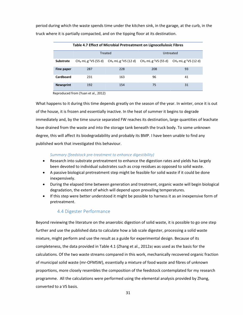
31
period during which the waste spends time under the kitchen sink, in the garage, at the curb, in the
truck where it is partially compacted, and on the tipping floor at its destination.
Table 4.7 Effect of Microbial Pretreatment on Lignocellulosic Fibres
Treated Untreated
Substrate CH4 mL.g-1VS (55 d) CH4 mL.g-1VS (12 d) CH4 mL.g-1VS (55 d) CH4 mL.g-1VS (12 d)
Fine paper 287 228 208 93
Cardboard 231 163 96 41
Newsprint 192 154 75 31
Reproduced from (Yuan et al., 2012)
What happens to it during this time depends greatly on the season of the year. In winter, once it is out
of the house, it is frozen and essentially inactive. In the heat of summer it begins to degrade
immediately and, by the time source separated FW reaches its destination, large quantities of leachate
have drained from the waste and into the storage tank beneath the truck body. To some unknown
degree, this will affect its biodegradability and probably its BMP. I have been unable to find any
published work that investigated this behaviour.
Summary (feedstock pre-treatment to enhance digestibility) Research into substrate pretreatment to enhance the digestion rates and yields has largely
been devoted to individual substrates such as crop residues as opposed to solid waste. A passive biological pretreatment step might be feasible for solid waste if it could be done
inexpensively. During the elapsed time between generation and treatment, organic waste will begin biological
degradation, the extent of which will depend upon prevailing temperatures. If this step were better understood it might be possible to harness it as an inexpensive form of
pretreatment.
4.4 Digester Performance
Beyond reviewing the literature on the anaerobic digestion of solid waste, it is possible to go one step
further and use the published data to calculate how a lab scale digester, processing a solid waste
mixture, might perform and use the result as a guide for experimental design. Because of its
completeness, the data provided in Table 4.1 (Zhang et al., 2012a) was used as the basis for the
calculations. Of the two waste streams compared in this work, mechanically recovered organic fraction
of municipal solid waste (mr-OFMSW), essentially a mixture of food waste and fibres of unknown
proportions, more closely resembles the composition of the feedstock contemplated for my research
programme. All the calculations were performed using the elemental analysis provided by Zhang,
converted to a VS basis.

32
Four calculations generated the key data to measure digester performance; the calculations are
presented in Fig. 4.2.
a) The stoichiometric formula of mr-OFMSW, from the elemental analysis, was found to be
C 29.4 H51.3 0 14.9N.
b) Stoichiometric calculations were performed using the appropriate organic half reactions, the
fraction of electrons to cell synthesis (fs) equal to 0.08 for low-yield anaerobic processes, and
C5H7O2N as the formula for new cells (Rittmann & McCarty, 2001). They showed that, at 70% VS
destruction, mr-OFMSW would produce 377 LCH4.kg-1VSadded. By comparison, Zhang’s measured
BMP was 364 LCH4.kg-1VSadded; this suggests that 70%VS destruction is a good working estimate.
c) The energy balance was calculated using a modified form of Dulong’s law; the modifications
were based upon an extensive analysis of the elemental composition and calorific value of
OFMSW (Komilis et al., 2012); this source was chosen specifically because the work
concentrated on substrates of interest. The energy content of the VS destroyed (16.00 MJ)
balanced with the energy content of the CH4 + biomass produced (15.66 MJ), to within 2%.
d) The rate calculations were based on a pseudo-parallel first-order kinetic model and rate
constants developed by Zhang (2012a):
𝑦 = 𝑦 1 − 𝑃𝑒 − (1 − 𝑃)e (4.1)
Where y = cumulative methane yield at time t, ym = ultimate methane yield, k1 and k2 are the first-
order rate constants for the proportion of readily and less-readily degradable material respectively, and
P is the proportion of readily degradable material. By using this expression it was possible to estimate
the short-term and longer-term biogas generation rate from mr-OFMSW. The rate calculations indicate
initial biogas production rates of 8L to 11 L.h-1.kg-1VSadded in the first hour, 5.8 to 8.2 L.h-1.kg-1VSadded in
the first 24h, and an ultimate yield of 343 to 349 L.kg-1VSadded after 42 days; in each case, the spread
represents the difference between P = 0.3 and P = 0.5; the higher rate corresponding to the higher
fraction of readily degradable waste. The calculated and experimental yields from published sources
are summarized in Table 4.8.

33
Table 4.8 Biochemical Methane Potential L CH4.kg-1VSadded
Calculated from equation (1)
P = proportion of readily degradable material Experimental Results
P = 0.3
mr-OFMSW
P = 0.5
mr-OFMSW
Zhang
mr-OFMSW
Zhang
ss-MSW
Bolzonella
ss-OFMSW
Abassi-Guendouz
Cardboard
Buffiere
Cardboard
343 349 344 445 400 176 240
a) Stoichiometry Based on data from Table 4.2.1 the stoichiometric equation for the digestion of mr-OFMSW is: 7.3C 29.4 H51.3 0 14.9N (656.5)+63H2O (18) = 4C5H7O2N (113)+115CH4 (16)+77CO2 (44) +3NH4
+ (18)+3HCO3- (61)
(MWT in parentheses) b) Methane Yield
i. Converting the stoichiometric equation to mass in g; 4792g C 29.4 H51.3 0 14.9N + 1134g H2O = 452g C5H7O2N + 1840g CH4 + 3388g CO2 + 54g NH4
+ + 182g HCO3-
ii. Converted to 1kg of VS basis gives: 1000 + 237 = 94.3 + 384 + 716 + 11.3 + 38.0
1237g ≃ 1244g
iii. CH4 = 16/22.412 L.g-1 → 384g/0.714 g.L-1 = 538L CH4 or, at 70% VS conversion, 377L CH4, iv. CO2 = 44/22.412 L.g-1 → 716g/1.96 g.L-1 = 365l CO2 or, at 70% VS conversion, 256L CO2. v. Methane content = 538/(538 + 365) x 100 = 59.6% CH4.
Theoretical yield = 538l CH4 and 903L biogas per kgVSadded At 70% VS conversion yield = 377L CH4 and 632L biogas per kgVSadded
c) Energy Balance Using modified Dulong formula (Komilis et al., 2012) Energy content:
i. mr-OFMSW = (341.9C+1272H-149.6O)/1000 = (341.9x53.6+1272x7.8-149.6x36.1)/1000 = 22.85MJ.kgVS-1 ii. Biomass = (341.9x53.0+1272x6.2-149.6x28.3)/1000 = 21.77MJ.kgVS-1
iii. CH4 = 37.78MJ.m-3 iv. Biogas @ 59.6% CH4 = 22.5 MJ.m-3 v. 632l biogas = 14.22MJ
vi. 94.3 x 0.7g biomass created = 1.44MJ vii. Total e) + f) = 15.66MJ
viii. 0.7kgVSdestroyed = 16.00MJ d) Methane Production Rate (from BMP)
𝑦 = 𝑦 1 − 𝑃𝑒 − (1 − 𝑃)e
ym = 364 L.kgVS-1added, P = 0.32 or 0.3, k1 = .77 and k2 = 0.05
Calculation performed at P = 0.3 and P = 0.5 and methane converted to biogas yield at 59.6% CH4 gives: i. 𝒚 = 7.8L biogas at 1 hour, 140L at 1 day and 343L at 42d (L.kgVS-1
added at P = 0.3) ii. 𝒚 = 11.2L biogas at 1 hour, 196L at 1 day and 349L at 42d (L.kgVS-1
added at P = 0.5)
Figure 4.2 Digester performance calculations from first principles. a) Stoichiometry of mr-OFMSW digestion; b) Theoretical methane yield at 70% VS conversion; c) Energy balance: COD destroyed vs. (CODout biomass + CODout CH4 ) d) Estimates of biogas production at 1h, 24h and 42d.
34
Summary (Digester performance) Based on published data and these calculations of methane yield, the experimental digester
would be expected to produce between 100 and 450 L CH4.kg-1VSadded, depending upon the mixture of substrates fed.
In a batch-fed system, the rate of biogas production will rise quickly, immediately after fresh waste is added, and then steadily decline in a manner determined by the fraction of readily-digested waste added.
The initial rate of biogas production could reach 11 L.h-1.kg-1VSadded and, making allowances for potential errors in this estimate, provision should be made to accommodate a peak biogas production rate of 15 L.h-1.kg-1VSadded.
The methane content of the biogas produced, depending on the specific mix of substrates, could reach 60%.
Approximately 65% of the VS fed to the reactor (349 L.kg-1VSadded/377 L.kg-1VSadded*70%) can be expected to be converted to biogas.
4.5 Aerobic Curing
The anaerobic digestate will not be biologically stable, may still contain pathogens, and may be
odorous; aerobic curing therefore is the necessary final step of the process (Brinton, 2006; Pognani et
al., 2012; Yazdani et al., 2012). Pognani et al. (2012) present a complete mass balance of the combined
anaerobic/anaerobic treatment plant for OFMSW, based on one year of operation of the DRANCO
technology. The digestate was mixed with wood chips and aerobically composted in a tunnel system for
one week, under forced air conditions. At the end of this phase the partly composted digestate was
placed in piles, which were turned twice per day for a further 1 to 2 weeks. The final compost product
was screened and the recovered bulking agent returned to the process; the end-product was sterile and
suitable for land application.
Yazdani (2012) describes an anaerobic/aerobic landfill-based digester, using 1.7 tonnes of yard waste as
the substrate, ultimately producing a finished compost. The process was carried out in three stages;
filling (93 days), anaerobic digestion (366 days) and aerobic curing (191 days). During the curing process
methane continued to be produced because not all the waste mass had turned aerobic, but most of the
methane was removed by the biofilter. At the end of the aerobic curing, the composted product was
recovered and tested and found suitable for land application; one of the recommendations for future
design and operation was to shorten the aerobic curing period.
Summary (Aerobic curing) Aerobic curing (composting) of digestate is required. Composting can be carried out in situ or ex situ or some combination of both. The planned use of bulking agent to aid anaerobic digestion will also assist in the aerobic
curing.

35
Recovery and reuse of bulking agent is feasible. A good quality compost requires clean feedstock. Composting is a logical complement to anaerobic digestion.
4.6 Conclusions and Knowledge Gaps
The findings of the literature review confirm that it should be possible, within limits yet-to-be-defined,
to digest mixed wastes comprising food waste plus lignocellulosic fibres in varying proportions. The
food waste portion will digest rapidly and the fibres less rapidly; surges in biogas from freshly-fed waste
(particularly food waste) are expected, and could rise as high as 11L.h-1.kg-1VSadded as the easily-digested
FW is converted; this will then subside as the more recalcitrant substrates are digested. Digestibility of
the waste will range from 30% to 80% but probably, on average, be around 65%, depending on the mix.
Management of the C:N ratio, alkalinity and pH will reduce the risk of process instability or inhibition.
Some size reduction of the substrates will be necessary to improve uniformity. Maintaining a high
moisture content within the waste mass, which must remain permeable, is critical; a total solids
content between 20% and 25% would appear to be a good place to start. A final composting step to
cure the digestate is necessary to achieve stability and sterilization and produce a usable product.
In the course of this review, several notable gaps in the literature were identified. First and foremost no
extensive studies were found that were specifically designed to test the co-digestion of food waste with
lignocellulosic fibres arising from the paper and cardboard products in the solid waste stream.
Secondly, no attempt has been made to study the stability and performance of an anaerobic digester
treating any waste streams of variable composition over an extended period of time. As a consequence,
a digester specifically intended for this purpose has not been built, and a suitable design concept has
yet to be defined. While management of the C:N ratio and digester pH and alkalinity are proven tools to
manage digester stability, their suitability in a system with variable feedstock composition is unknown.
Given the heterogeneous nature of the wastes to be studied, and the probable presence of foreign
matter, the preferred approach is solid state anaerobic digestion (SS-AD), whereby the waste remains
stationary and has leachate percolate through it. The system would take the form of a two-stage
anaerobic digester, comprising sequentially fed leach beds plus a UASB operating at mesophilic
temperatures, to be followed by an aerobic curing step. This arrangement would conform to the
concept of the BioPower process.
A combination of cardboard, boxboard, newsprint and fine paper (CB, BB, NP and FP) collectively fibre
(FB), plus food waste (FW), will serve as a suitable proxy for the organic fraction of commercial solid
waste. Bulking agent in the form of woodchips will be required to ensure continued permeability in the
36
leach beds. A portion of the FW will digest very rapidly; the balance will digest more slowly. The CB, BB,
NP and FP, and the BA will all be relatively slow to digest, depending upon their respective lignin
contents.
FW alone has a low C:N ratio and is always susceptible to process instabilities caused by high VFAs and
resultant low pH, or high ammonium, or alternate between these conditions. The presence of FB will
raise the C:N ratio and thereby stabilize the digester.
Co-digestion of two or more substrates has been shown to enhance digester performance; digestion
rates and yields can be increased and stability enhanced. FW has been widely studied as a co-substrate
but usually with waste-water sludges or crop residues. The co-digestion of FW with the fibres found in
solid waste, under conditions of varying FW addition, is essentially unexplored.
Some feedstock preparation will be necessary. Following the principles established in Section 2.1, this
will be kept to a minimum and consist primarily of pre-sorting the FW to remove undigestible
contaminants, plus some size reduction of the FB.
Digester performance, measured as the rate and yield of methane production, is expected to vary
considerably depending upon the level of FW addition. A range of 100 to 450 L CH4.kg-1VSadded is
expected. After fresh substrate has been introduced a rapid rise in biogas production, to perhaps
11 L.h-1.kg-1VSadded, is expected.
Digester stability can be achieved by monitoring and controlling the C:N ratio, pH, alkalinity ratio, VFA
concentration and ammonia concentration. The suitability of these methods is well-documented for a
digester that has only been fed with food waste of consistent composition. But their effectiveness for
monitoring and controlling the digestion of variable feedstocks is unknown.
The behaviour of the microbial community may be able to provide insight into the process, but how
that knowledge can be developed and applied in a practical sense, has yet to be determined.
Thus there remain several important knowledge gaps; questions which the literature cannot fully
answer, specifically:
1. How does the C:N ratio vary in response to the range of waste compositions contemplated by
this research and what does this imply for process performance and stability?
2. How coarse can the substrates be before channelling begins in the leach beds?
3. How does the preparation of the bulking agent affect digester performance?

37
4. What is the effect on process stability of short-term (week to week) and longer term (month to
month) changes in the proportions of FW and FB?
5. To what extent does the addition of FW enhance the digestibility of recalcitrant substrates such
as FB’s, compared to a baseline without FW?
6. What are the benefits of using sequentially-fed leach beds compared to other AD technologies;
can they be quantified?
7. Are pH and alkalinity, VFA concentration and C:N ratio adequate tools to control the AD process
in this application, and how can they be used to greatest advantage?
8. How tolerant is the UASB of the properties and variability of the leachate fed to it, and what are
the preferred operating conditions of OLR, HRT and Vup?
9. What proportion of the biogas is generated in the leach beds and how does the gas production
vary with time as the digestion process progresses?
10. How does the microbial population respond to changes in feedstock composition, does it
become more diverse and robust?
11. How effective is aerobic curing of the digestate; how long does it take, and what is the quality
of the product?
12. What are the key operating variables to be monitored and controlled, and what are their
preferred operating ranges in a digester processing mixed solid wastes?
13. In what ways and to what extent can the experimental results be used to design a pilot-scale or
full-scale digester?
These are the questions which this research programme sets out to investigate and answer, and since
part of the proposed research involves simulating the real-world variability of solid waste, devising a
reliable design and operating plan to control the process will be particularly important.

38
Chapter 5. Digester Design and Construction
In this Chapter a design concept is described with reference to the BioPower process, then refined,
major component by major component, with further reference to the literature. The final result is a
refined design concept ready for procurement and construction.
5.1 Design Basis
The relationships among biochemistry, process operating conditions, feedstock properties, and digester
performance are at the heart of the engineer’s challenge when designing, building, and operating an
anaerobic digester for solid waste. Simply put, the objectives are to achieve rapid substrate destruction
and methane formation, with the minimum amount of energy input, and without causing reactor
instability. This will be a constant theme throughout this work. The wastes that concern us in this
project are of two types, food waste and lignocellulosic fibres. The lignocellulosic fibres, namely
cardboard (CB), boxboard (BB), newsprint (NP), and fine paper (FP) - collectively called fibres (FB) are
derived from wood, the food waste comes from a green bin program. It was decided to use a bulking
agent (BA) in the form of woodchips to enhance the permeability and porosity of the substrates. For
convenience, the BA is included in this section as a substrate. The rationale and methodology for the
use of BA is covered in Section 4.3.3. The principal objective was to determine what is known about the
intrinsic properties of the chosen substrates, individually and collectively, and how they behave in the
anaerobic digestion process. One of the underlying principles of the BioPower process is the
employment of solid state anaerobic digestion (SS-AD) to avoid these complications and costs, so the
“wet” versus “dry” decision has, in effect, already been made.
Given the versatility and apparent advantages of two-stage digestion, particularly with more easily
digested waste (such as food waste), I chose two-stage digestion, using leach beds for the first stage
and a UASB for the second stage. The choice of a UASB over other methanogenic reactors, such as
anaerobic filters or CSTRs, was for reasons of practicality, simplicity and cost. The final design made it
possible to operate the digester with or without the UASB though, in practice, it remained in operation
throughout.
I also selected mesophilic temperatures, partly for practical reasons associated with heating a lab scale
reactor, but also because the literature did not provide strong arguments for choosing thermophilic. A
comparison of mesophilic and thermophilic digestion with substrates containing cellulose and
hemicellulose found that, while the reaction rate at thermophilic temperatures was greater, the
digester was prone to surges of VFAs resulting in reactor instability (Shi et al., 2013).
39
There was one additional constraint which affected the design of the experimental digester. Because
the system would be producing methane gas and trace amounts of hydrogen sulfide, it had to be
constructed in a walk-in fume hood. This imposed a practical upper limit on the volumetric capacity of
the system, and had a great influence on the ultimate layout.
Only certain aspects of reactor design are discussed in the literature. These are principally the capacity,
dimensions, and operating conditions of leach beds and of UASBs. In the initial stages of planning, I
received fortuitous assistance from Abdul-Sattar Nizami, a postdoctoral fellow in the Department of
Department of Chemical Engineering and Applied Chemistry. Nizami’s PhD research and associated
publications centred around the SS-AD of grass silage in a two-stage digester consisting of six
sequentially-fed leach beds and a UASB. In several discussions we reviewed his design, the logic behind
it, the operational difficulties he had encountered, and how he dealt with them; he provided me with
engineering drawings of his system. We also held a video conference call with James Browne who had
adapted Nizami’s digester to process source-separated food waste. Browne had run into numerous
difficulties; low yield (compared to the grass silage for which the system had been designed), a large
accumulation of ammonium ions, made worse by rising pH (ammonia being more inhibitory than
ammonium), an increasing recirculating load of inorganic salts, foaming in the UASB and an
accumulation of fines plugging the leach beds. The C:N ratio, at 14:1, was low and this certainly
contributed to the problems encountered. A review of the published papers by Browne & Murphy
(2013; 2014) describe some of these difficulties, but not in the graphic detail of our conference call.
I adopted the design of Nizami et al.(2011) as a template, to be altered and refined, as appropriate, to
suit my substrates, and the results of a further review of the literature dealing with other examples of
this kind of digester configuration.
5.1.1 Leach Beds
The purpose of the leach bed is to provide intimate contact between the solid substrates and the
leachate, which contains nutrients and the microbial community; typically the goal is to effect
hydrolysis of the substrates followed by acidogenesis in the leach bed. The design has to achieve three
things; even distribution of the leachate over the entire cross section, a long pathway for leachate
percolation, and the ability to retain as many of the fines as is practical, all of this to be accomplished
while minimizing wall effects.
The literature contains few examples of the use of multiple leach beds for the digestion of solid waste.
Chugh et al. (1999) used a combination of two leach beds operating in series, one with fresh waste, one

40
with stabilized waste, to accelerate the digestion of MSW; they achieved 75% degradation of the
rapidly biodegradable fraction within two months. In an earlier paper, O'Keefe et al. (1993) also
digesting MSW, operated three leach beds labelled “new”, “mature”, and “old”. The mature leach bed
recirculated leachate only within itself, while the new and old were interconnected and recirculated
leachate between them; 49.7% of VS was degraded in 42 days. To digest food waste, Han (2004)
operated four leach beds in parallel connected to a UASB, achieving 80.5% VS reduction in two days;
the experiment ran for 110 days. Using the same experimental system, Shin (2001) achieved 85% VS
reduction in 10 days in an experiment that ran for 150 days. In neither case did they experience any
process instability. Yet Browne et al., also digesting food waste alone in a similar system, ran into
serious instability problems; the difference would appear to be that Han and Shin diluted the leachate
in the system every 10 days to lower the ammonia concentration, while Browne did not. This further
highlights the challenges of digesting food waste by itself, as discussed in Section 4.2.1. A summary of
reactor volumes, biogas yields, and SRTs from leach bed digestion experiments performed on organic
waste and related substrates is presented in Table 5.1. The clear outlier of this group is the work of
Eleazer et al. (1997) whose aim was to study anaerobic decomposition of organic waste under
simulated landfill conditions, using well digested solid waste as the inoculum. Of the remaining studies,
Murto et al.’s (2013) substrate was the recalcitrant portion of OFMSW, containing mostly lignocellulosic
materials.
Based on all these data, I decided on an initial SRT of 42 days. Using the conceptual design of six leach
beds, each would have sufficient capacity to hold a mixture of saturated substrates weighing
approximately 6 kg (about 8.5 L), for a total of 36 kg wet weight at about 30% TS and an aggregate
working volume of about 50 L. This arrangement would require the removal and replacement of one
leach bed per week, which I thought operationally manageable. It also meant that each charge of fresh
waste would represent only 16% of the total mass within the digester, the balance providing
operational buffering, presumably enhancing digester stability. Also, with careful design of the piping
and valves, operation with fewer leach beds would be feasible, if this were necessary or desirable.
To meet the objective of evenly distributing the leachate over the cross-section of a leach bed, a
delivery system was required. The only information I could find in the literature was the description of
gravity-drained leachate cups (Nizami et al.,(2011).

41
Table 5.1 Leach Bed Digestion - Performance Data Substrate Reactor Leach bed
working capacity (L)
SRT (d)
Biogas yield L CH4.kgVS-1
added Comments Source
Maize Leach bed + UASB
4.0 28 540 (Cysneiros et al., 2012; Cysneiros et al., 2011)
Food waste Leach beds + UASB
17.0 24 340 (Browne et al., 2013)
Dry fraction OFMSW
Leach bed + UASB
5300 74 233a Mostly lignocellulo
sic
(Murto et al., 2013)
Food waste Leach beds + UASB
35.0 10 270 (Han et al., 2002)
MSW Multiple Leach beds
400b 35 270 Bekon system
(Qian et al., 2016)
Grass silage Leach beds + UASB
17.0 30 - 42
341 optimized (Nizami & Murphy, 2011)
Food waste Leach bed 2.0 180 320 Landfill simulation
(Eleazer et al., 1997) Newsprint Leach bed 2.0 430 75.4 Cardboard Leach bed 2.0 470 155 Fine paper Leach bed 2.0 680 288 MSW Leach bed +
UASB 14.0 20 85 Landfill
simulation (O'Keefe &
Chynoweth, 2000) aestimated from kgTS-1added. bm3.
When these are full, a level sensor activates a solenoid valve causing them to drain into the leach bed
through a sprinkler system. This arrangement was plagued with problems, mostly caused by the
presence of suspended particulate matter that both fouled the sensor and partially plugged the
sprinkler system. Direct injection appeared to offer greater reliability than gravity delivery; a closed
loop, to constantly circulate leachate through a manifold above the leach beds and back to the tank,
was designed. Pneumatic solenoid valves, opening automatically on a signal from a programmable logic
controller (PLC), would redirect the flow to each leach bed in turn. Thus the potential for plugging
would be greatly reduced and constant volumes of leachate always delivered. A method to ensure the
even distribution of leachate required some thought and experimentation. All methods employing any
form of nozzle or orifice with leachate under pressure, would operate differently at different flowrates
and be subject to plugging and failure. Relying on drainage through a plate with holes in it would be
subject to plugging, and also to uneven settlement of the substrate, resulting in maldistribution of the
leachate. The method chosen uses a 4mm thick non-woven geotextile (TenCate Mirafi 1600N). In a
simple bench test, 500 mL per minute of water was delivered onto a 15 cm geotextile disc; the water
was found to be reliably distributed to the perimeter before completely draining through. Once fresh
waste was loaded into a leach bed, a geotextile disc was placed on top covering about 80% of the cross-
sectional area. This technique was used throughout and worked very well.
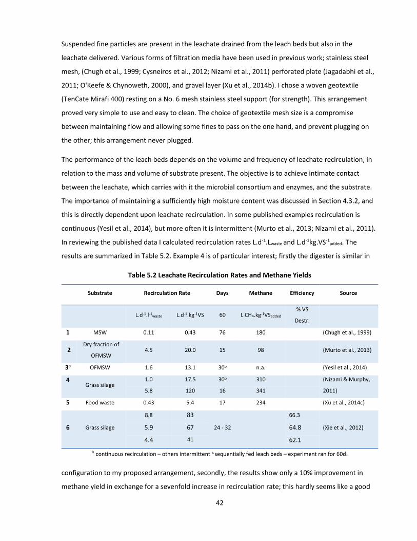
42
Suspended fine particles are present in the leachate drained from the leach beds but also in the
leachate delivered. Various forms of filtration media have been used in previous work; stainless steel
mesh, (Chugh et al., 1999; Cysneiros et al., 2012; Nizami et al., 2011) perforated plate (Jagadabhi et al.,
2011; O'Keefe & Chynoweth, 2000), and gravel layer (Xu et al., 2014b). I chose a woven geotextile
(TenCate Mirafi 400) resting on a No. 6 mesh stainless steel support (for strength). This arrangement
proved very simple to use and easy to clean. The choice of geotextile mesh size is a compromise
between maintaining flow and allowing some fines to pass on the one hand, and prevent plugging on
the other; this arrangement never plugged.
The performance of the leach beds depends on the volume and frequency of leachate recirculation, in
relation to the mass and volume of substrate present. The objective is to achieve intimate contact
between the leachate, which carries with it the microbial consortium and enzymes, and the substrate.
The importance of maintaining a sufficiently high moisture content was discussed in Section 4.3.2, and
this is directly dependent upon leachate recirculation. In some published examples recirculation is
continuous (Yesil et al., 2014), but more often it is intermittent (Murto et al., 2013; Nizami et al., 2011).
In reviewing the published data I calculated recirculation rates L.d-1.Lwaste and L.d-1kg.VS-1added. The
results are summarized in Table 5.2. Example 4 is of particular interest; firstly the digester is similar in
Table 5.2 Leachate Recirculation Rates and Methane Yields
Substrate Recirculation Rate Days Methane Efficiency Source
L.d-1.l-1waste L.d-1.kg-1VS 60 L CH4.kg-1VSadded
% VS
Destr.
1 MSW 0.11 0.43 76 180 (Chugh et al., 1999)
2 Dry fraction of
OFMSW 4.5 20.0 15 98 (Murto et al., 2013)
3a OFMSW 1.6 13.1 30b n.a. (Yesil et al., 2014)
4 Grass silage
1.0 17.5 30b 310 (Nizami & Murphy,
2011) 5.8 120 16 341
5 Food waste 0.43 5.4 17 234 (Xu et al., 2014c)
6
Grass silage
8.8 83
24 - 32
66.3
(Xie et al., 2012)
5.9 67 64.8
4.4 41 62.1
a continuous recirculation – others intermittent b sequentially fed leach beds – experiment ran for 60d.
configuration to my proposed arrangement, secondly, the results show only a 10% improvement in
methane yield in exchange for a sevenfold increase in recirculation rate; this hardly seems like a good

43
bargain; it is operationally impractical in the lab and financially burdensome on a commercial scale. In
Example 6, also a study of the effects of leachate recirculation rate on the hydrolysis of grass silage, the
recirculation rates are similar to those of Example 4, but also show that a doubling of the recirculation
rate yields only a 7% increase in VS destruction. Example 2 is from a large-scale experiment (3 tonnes of
substrate) using wood chips as a bulking agent. In general, higher recirculation rates seem to produce a
higher methane yield, and greater VS destruction. The review of solids content (Section 4.3.2) showed
that when the moisture content is too high, digester performance deteriorates. There is also the
practical question of how the actual substrate used in the proposed experiments would behave; for
example how much moisture would a leach bed of solid waste hold, and how quickly would it drain? I
decided to design the system with a lot of flexibility and provide for a recirculation rate ranging from
5 to 20 L.d-1.kgVS-1added. The frequency and duration of leachate recirculation would be determined
experimentally.
Summary (Leach bed design) the digester will have six leach beds (plus a seventh to simplify removal and replacement) each leach bed will have a working volume of about 8.5 L. the waste will be supported on a No. 6 mesh stainless steel screen mounted in the bottom. the loss of fines will be minimized by a woven geotextile filter sitting on the screen. a nonwoven geotextile will be placed on top of the waste to distribute the incoming leachate
over the cross-section of the leach bed. initial leachate recirculation rate will be between 5 and 20 L.d-1.kgVS-1
added. the frequency and duration of leachate delivery to the leach beds will be determined
experimentally. the question of whether or not to provide external heat for the leach beds, and if so how,
remained unresolved at this point.
5.1.2 Upflow Anaerobic Sludge blanket (UASB) Reactor
Mechanically, the UASB reactor is a simple piece of equipment with no moving parts (other than a feed
pump). It is capable of converting soluble COD at a high organic loading rate (OLR), and does not
require a lot of space. It does require supplementary heating and thermostatic control to maintain a
steady operating temperature of about 37°C. The logic behind the choice of OLR, HRT and Vup is
thoroughly explained in the literature (Campos & Anderson, 1992; Goncalves et al., 1994; Lettinga &
Pol, 1991); all of them are older publications from the early days of UASB development. More
specifically, a review paper on the application of UASBs for waste water treatment by Latif et al. (2011)
provides a summary of published information on the design and operation of UASBs in many different
applications. OLRs range from 0.77 to 30 gCOD.L-1.d-1, HRTs from 2.4 to 480 h and upflow velocities (Vup)
from 0.0018 to 2.0 m.h-1. These are very wide ranges, but by eliminating designs which lacked

44
supporting data, or did not work well, and by examining the specific applications, it was possible to
narrow the ranges substantially; OLRs from 3 to 14 gCOD.L-1.d-1, HRTs from 5.0 to 48 h and Vup from 0.1
to 0.6 m.h-1. These were adopted as the design operating ranges. For comparison purposes,
experiments with grass silage were conducted using an OLR of 6 gCOD.L-1.d-1, an HRT of 7.5 h, and a Vup
of 0.1 m.h-1 (Nizami et al., 2011).
Table 5.3 summarizes the most useful published information on the capacity and aspect ratios of leach
beds and UASBs, and the volumetric relationship between them. Reactor dimensions vary widely and
analyzing this information is made difficult by the complete lack of explanation in the literature on how
the chosen dimensions were arrived at. Though one thing is certain; Jagadabhi et al.’s (2011) UASB was
greatly undersized for FW digestion; it was unable to cope with the OLR, and had to be uncoupled from
the LB. For my proposed digester, comprising six leach beds of 50 L working volume in total, using a
Table 5.3 Leach Bed and UASB Dimensions
Substrates Leach beds UASB Vol. ratio Source
d(cm) h(cm) v(L) # h/d d(cm) h(cm) v(L) h/d LB/UASB
1 MSW 20 44 14 1 2.2 15 29 5 1.93 2.8 (O'Keefe & Chynoweth, 2000)
2 MSW 200 2 (Lai et al., 2001)
3 ss-FW 4.5 1 3 1.5 (Wang et al., 2003)
4 Grass silage 38 15 16 6 0.4 23 75 31 3.3 3.1 (Nizami et al., 2011; Xu et al., 2011)
5 FW 4.6 1 10 1.8
(Jagadabhi et al., 2011; Xu et al., 2011)
6 Crop
residue and FW
10 1 0.5 1.0 20.0 (Jagadabhi et al., 2011)
7 Maize 13 30 3.5 1 2.3 6.2 50 1.5 8.0 2.7
(Cysneiros et al., 2012; Cysneiros et al., 2011)
8 Grass silage 9.2 30 2.0 1 3.3 (Xie et al., 2012)
9 Landfill leachate
15.6 26 5 1.67 (Kennedy & Lentz, 2000)
10 FW (cafeteria)
19 38 8.0 4 2.0 *20 and *32
*80 and *20
41 1.9 0.8 (Shin et al., 2001)
11 FW + FB 20 26 8.5 6 1.3 25 55 27 2.2 1.9 This study
*lower and upper sections of different diameters
45
LB:UASB volumetric ratio of 0.8 (Example 10) gives a UASB volume of 63 L, and using a LB:UASB
volumetric ratio of 3.1 (example 4) gives a UASB volume of 16 L. The aspect ratio (h:d) of UASB reactors
shows a range of 1.7:1 to 8:1. Meyer (2013) used 6.8:1 with a working capacity of 5.4 litres, and Nizami
et al. (2011) used 3:1 with a working capacity of 31.4 L.; the most relevant data found in the literature
are shown in Table 5.3. It is possible that the specific dimensions are much less important than the
combination of OLR, HRT and Vup. Accordingly, the UASB was designed and built in two sections of
unequal length, so that it could be operated either as a single combined unit, or as one of two smaller
units, with approximate capacities of 20 L, 30 L or 60 L. This combination allowed operation at a
LB/UASB ratio from 0.8 to 3.1, covering the entire range in Table 5.3 (with the exception of Example 6
which was included as an example of a poor design). Furthermore, by selecting the appropriate
peristaltic pump and tubing, the HRT and Vup could be set anywhere within the preferred ranges.
To operate the digester as a closed system, the UASB effluent must be discharged to the storage
tank(s). Table 5.3, Example 11, shows the dimensions finally used.
Summary (UASB design) the UASB will be constructed in two sections of unequal length with a maximum combined
capacity of approximately 60 L. it will be operable at capacities of about 20 L, 30 L or 60 L depending on the configuration
chosen. a peristaltic pump and tubing will be chosen to achieve an HRT from 5.0 to 48 h and a Vup from
0.1 to 0.6 m.h-1. leachate inflow will be distributed with a No. 6 mesh stainless steel screen mounted the
bottom of the UASB. the UASB will be supplied with external heat and thermostatic control.
5.1.3 Leachate Tanks
Leachate storage in a heated, thermostatically controlled tank is required to;
supply leachate and heat, to the leach beds.
receive the leachate drained from the leach beds and
supply leachate to the UASB.
maintain hydraulic and thermal balance.
The required capacity for this storage is a function of the volume of substrate in the leach beds, the
recirculation rate, the leachate retention capacity of the waste, and the required flow rate to the UASB.
In particular, intermittent delivery of leachate to the leach beds draws down the contents of the
storage tank, and is only replenished when the leachate percolates through the waste and returns to
the tank; during this period the UASB must not be starved of flow. There is very little information in the

46
literature to guide the decision on tank capacity. Nizami et al (2011) operated with a 40 L tank,
representing 31% of the combined volume of a 31 L UASB and 96 L of waste in the leach beds. Murto et
al. (2013) operated with a 700 L tank representing 9% of the combined volume of a 2.6 m³ anaerobic
reactor and 5.3 m³ of waste in the leach bed. Based on the available information, I concluded that
leachate storage capacity of about 40 L would be required. The question of whether this should be
provided using one or more tanks was unresolved at this point. There is one other factor to be
considered; a UASB works very well for soluble COD, but less well for suspended COD (Lettinga & Pol,
1991). Suspended matter is certain to be present in the storage tanks, and it would be desirable to
install a weir to restrict the flow of particulate matter to the UASB, but then what steps would be
needed to prevent sludge accumulation in the tank(s)?
Summary (Leachate tanks) leachate storage of about 40 L is required. it could be a single tank or perhaps two tanks. the tank(s) must be heated and thermostatically regulated. it would be advantageous to install a weir or clarifier in the storage tank. some mechanism for preventing sludge accumulation would then be required.
5.1.4 Biogas Production
Nizami et al. (2010) only measured biogas from the UASB, not from the leach beds, apparently because
virtually all the biogas was produced in the UASB. Accordingly, the original intention was to install a
single gas meter at the outlet from the UASB and connect in the headspace from the tank(s) and the
leach beds to capture any biogas that they might contribute, and to maintain hydraulic balance.
However, a further review of the limited information available in the literature suggested that the
principal source of the biogas would depend upon digester conditions, principally pH, and might in fact
come primarily from the leach beds. Murto et al. (2004) digesting mr-OFMSW ran two experiments,
each for 74 days, each with a combined single leach bed and methane reactor; bulking agent was added
to the first, but not to the second. With bulking agent added, 75% of the biogas came from the leach
bed; without bulking agent 23% came from the leach bed and the digester produced 43% less biogas in
total. Shin et al. (2001) digesting food waste, acknowledged that biogas is produced in the leach beds,
and made an aggregate measurement of the total biogas produced. Chugh et al. (1999), digesting
MSW, operated two leach beds in series, one of fresh waste and the other of stabilized waste. Fresh
waste leachate had a starting pH of 4.2, but 10 days of leachate recirculation through stabilized waste
caused the pH to rise to 6.5. At this point the fresh waste leach bed was uncoupled from the stabilized
waste leach bed, and leachate was recirculated from and to the fresh waste leach bed. During the initial
10-day period the majority of the biogas was generated from the stabilized waste. Thereafter it was
47
generated from the fresh waste. It appeared that the source of biogas generation might vary with
experimental conditions so the decision was made to devote one gas meter to the UASB and install a
second to measure gas from the balance of the system, otherwise important information about the
behaviour of the digestion process was going to be permanently lost.
Summary (Biogas measurement) biogas can be generated in any part of the system. the source depends upon prevailing digester conditions. it probably also depends upon the substrates. two gas meters are required to avoid loss of valuable data.
5.1.5 Aerobic Curing
The practical value of aerobic curing as part of a commercial operation has been recognized (Brinton,
2006). One example of combined anaerobic and aerobic processing, at a semi-commercial scale, used
an anaerobic digestion period of 366 days, followed by an aerobic curing period of 191 days to treat
yard waste (Yazdani et al., 2012).
The original plan for the experimental programme was to cure the digestate in the seventh, separate,
leach bed with an initial SRT of one week, as suggested by Pognani et al. (2012). In practice the quantity
of waste was found to be too small and heat losses too great to do this successfully. To solve this, all
the digestate retrieved over the course of the experiment (about 300 kg) was stored at 4°C then
aerobically cured in a single experiment conducted at Miller Waste Systems, using an aerated static pile
system designed and built for the purpose (Chapter 9).
5.2 Design and Construction
This section describes in detail the design and construction of the experimental anaerobic digester,
which was given the sobriquet Daisy, after Daisy the Cow (Jones, 2013). The original Daisy is a stuffed
specimen of a breed of long-horned Gloucester cattle, and is currently resident in the Gloucester Folk
Museum. She comes from the same breed used by Edward Jenner to develop the smallpox vaccine in
1796. Daisy was stuffed in 1935, by the same firm of taxidermists used by Charles Darwin for his
specimens. Her pedigree is impeccable.
The design of every component in Daisy was an iterative process; most were sketched in several
versions, and many factors had to be taken into consideration before final decisions were made. Only
the most important steps of this process are included in what follows.

48
5.2.1 Guiding Principles
The guiding criteria for the design are as follows
safe operation under all circumstances
flexibility and versatility of operation
ease of feeding
the capacity to hold as much waste as physical constraints allow
24 hour operation, seven days per week, most of the time unattended
automated only to the extent necessary for safe continuous operation
ability to handle the surges of biogas expected after fresh waste is added
The following principal topics are covered:
leach beds: number, volume, dimensions
leachate delivery system and volumes
leachate storage: number size and configuration of storage tanks
UASB: volume, dimensions
pumps: type, number and capacity
heaters: capacity and type
control system and datalogging
biogas measurement
5.2.2 Safety
Safety considerations were always the first priority in the design, construction and operation of Daisy. A
risk analysis was conducted prior to construction, and is attached in Appendix B. The maximum
concentrations of methane and hydrogen sulfide that would be produced were estimated using
published data and conservative assumptions. The only risk identified which could not be engineered
around was a general power outage or the potential failure of the fume hood fan, which could result in
elevated concentrations of CH4 or H2S. In either circumstance several hours would elapse before
hazardous conditions were reached, based on the conservative assumption that there would be no
natural draft in the fume hood. Draft tests were performed with the fume hood fan switched off, using
dry ice; these showed that there was sufficient natural draft to maintain in-flow to the fume hood in
the event of a fan failure or power outage. For greater security an H2S monitor was installed in the lab.

49
A spill containment tray was designed, and constructed from polycarbonate plastic, to cover the entire
floor of the walk-in fume hood; its capacity was calculated at 110% of the total volumetric capacity of
the system. The tubing in the peristaltic pumps was repositioned at the three week mark, and replaced
every six weeks, throughout the operating period. Electrical equipment was located outside the fume
hood to the greatest extent possible. Electrical connections within the fume hood were all taped and
shielded from splashed liquids. Hot electrical terminals in the control panel were also shielded to
prevent accidental electrical shocks.
The datalogger was set up so that it could be monitored remotely through an Internet connection, and
this I did at least twice daily for the entire operating period. On four or five occasions, when
information from the data logger indicated process malfunction, I was able to drive to the University
and restore normal operation within an hour. A WebCam was mounted inside the fume hood pointed
directly at the floor of the spill containment tray; other than a small water leak during commissioning,
Daisy operated without any process leaks.
5.2.3 General Description
The major components of Daisy consist of seven Leach beds, one aerobic and six anaerobic, six
automatic three-way valves, one UASB, two tanks, two gas meters, and three pumps. All these
components and their interconnections are shown in Figure 5.1.
P2
Gas Meter 1
Aerobic Curing
Tank 2
LB 2 Anaerobic
Week 5
LB 5 Anaerobic
Week 2
LB 6 Anaerobic
Week 1
LB 4 Anaerobic
Week 3
Air Gas Meter 2
Waste Water
Biogas
Leachate
Leachate
UASB effluent
LB 3 Anaerobic
Week 4
U A S B
Tank 1
Treatment and Disposal Land Application
Screened Solid Digestate
Renewable energy
P1
P3
Automatic 3-way valves
Figure 5.1 Schematic flow diagram

50
The six operating leach beds contain waste that varies in age from six weeks (LB1) to one week (LB6) as
indicated by the shading. As shown, assuming a six week SRT, LB1 is ready for removal and replacement
with a fresh leach bed.
The system operates as follows. Pump three (P3) transfers leachate from Tank 2 (T2) to the leach bed
feed manifold and back to T2 in a continuous loop. The programmable logic controller (PLC, Plate 10)
actuates each three-way valve in sequence, redirecting leachate flow to each leach bed in turn, for a
pre-set time. The programme incorporates a short time delay between the closure of one valve and the
opening of the next to prevent overlap. The timing and duration of leachate delivery can be changed by
uploading different programs to the PLC. The system operates continuously. Leachate percolates
through the waste mass in each leach bed, and flows to a common LB manifold, and thence directly
into T1.
Pump one (P1) transfers leachate from T1 to the UASB at a predetermined fixed rate. In the UASB the
leachate passes through a suspended bed of granular sludge to the overflow point near the top, where
it exits as treated effluent and drains by gravity back to T2. From T2 the leachate is transferred once
again to the leach beds, and the closed loop is complete.
Biogas is produced in the UASB, in the leach beds, and in the tanks. Biogas from the UASB exits through
gas meter 1 (GM1) and from the leach beds and tanks combined through GM2; this arrangement was
used throughout except for brief periods when particular experiments, or GM calibration, required
temporary changes. The gas meters are simple wet tip devices that measure biogas in 100 ml
increments. The hydraulic
behaviour of the leach beds and
the tanks are intimately
connected. The transfer of
leachate from T2 to the leach
beds is balanced by an exchange
of headspace volume. As a
result, the biogas produced in
both must be measured
collectively. Separate
measurement of biogas
production in the leach beds is
very difficult, and requires Plate 1 Daisy the Digester – Overall view showing main components

51
temporary isolation of individual leach beds from the rest of the system; this is discussed more fully in
Chapter 8. The same conditions do not prevail in the UASB where the liquid level is constant and biogas
production is connected to the UASB headspace only.
The entire system runs automatically; temperatures in all six leach beds, T1 and T2, the UASB and GM2
are measured with three-wire resistance temperature detectors (RTDs), and recorded in the data logger
every 15 minutes. The RTD was chosen for its accuracy and durability, and for its flexibility – each is
installed through a compression fitting which allows the depth of the detector to be adjusted. Each tip
of GM1 and GM2 is recorded, and summed every five minutes, and every hour, by the datalogger.
Figure 5.1 depicts the original design. Two significant changes were made as a result of initial operating
experience. Firstly, as noted previously, it was found that aerobically curing the digestate in a leach bed
simply did not work because composting temperatures could not be achieved within the relatively
small mass of material present. Secondly, wastewater storage was not required. It was fully expected
that, with the successive addition of fresh waste and the water that it contained, wastewater would
have to be drained from the system from time to time. This did not happen; throughout the 616 days of
continuous operation Daisy remained in almost perfect hydraulic balance, requiring no net addition of
water or withdrawal of leachate. Once this balance was confirmed, the wastewater tank was removed
from the system. Daisy the Digester in her final form is shown in Plate 1. The following sections describe
each of the major components in greater detail.
5.2.4 Leach Beds
To arrive at the right specifications and configuration of the leach beds required many design iterations.
The final design is shown in Figure 5.2. The body of the leach bed, the flat top and the conical bottom
were fabricated from 1/2 inch PVC pipe (20 cm ID) and 1/2 inch PVC sheet. The top and bottom flanges
were each drilled with eight 1/4 inch bolt holes. Each flange had a machined groove to hold a Viton o-
ring. Three solvent-welded supports lugs were installed at the bottom to support the stainless steel
screen and geotextile. The leachate outlet was tapped for a ¾” NPT leachate drain pipe. The top was
drilled to accommodate three bulkhead fittings for gas venting, leachate delivery, and the resistance
temperature device (RTD). The gas venting, leachate delivery, and leachate drain pipe fittings are all
quick disconnects, equipped with a shut off valve in each half. This prevented the ingress of air during
connection and disconnection, and permits pressure testing. The RTD connection is a simple three
pronged plug. The lid bolts are fitted with wing nuts for ease of removal and replacement. Plate 2
shows an installed leach bed and its associated three-way automatic valve.
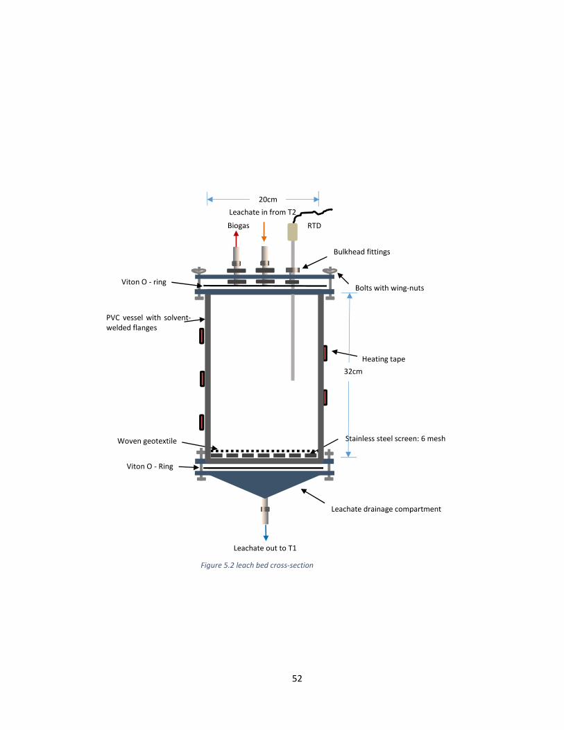
52
Heating tape
RTD
Bulkhead fittings
Leachate in from T2
Biogas out
Leachate out to T1
Bolts with wing-nuts Viton O - ring
PVC vessel with solvent-welded flanges
Woven geotextile
Viton O - Ring
Leachate drainage compartment
Stainless steel screen: 6 mesh
32cm
20cm
Figure 5.2 leach bed cross-section

53
The most important factors that contributed to the design were as
follows:
a) Dimensions and aspect ratio Nizami et al. (2010) used an aspect ratio of 0.4 - very wide and
flat as discussed previously. Although this had the advantage of
taking up less vertical space in the fume hood, it exacerbated the
problem of leachate distribution across the surface of the waste.
Since overall diameter was constrained by the available space in
the fume hood, I finally decided upon a ratio of 1.6 resulting in
dimensions of 20 cm d x 32 cm h to give a total volume of 10 L,
and a working volume of approximately 8.5 L. Diameter at the
flange was 27 cm.
b) Suspended particulate, fines and plugging This was the subject of several discussions. Nizami et al (2011)
and Browne et al. (Browne et al., 2013), treating grass silage and
food waste respectively, experienced serious plugging problems
with their two-stage digester system. After much thought, it
became apparent that:
fines would be produced in significant but unknown quantities.
they should be kept out of the UASB as far as possible they should not be
allowed to accumulate in the tanks - as far as possible.
they should not be allowed to settle in the piping system - as far as possible.
and that the best way to accomplish all this was to:
keep the leachate moving at all times
use the leach beds as a filter
incorporate a clarifier in the leachate tank (thank you Torsten Meyer)
flush the leachate lines regularly by temporarily raising pump speeds.
For the LB to function as a filter, the contents must of course remain permeable; the addition of
BA and the installation of geotextiles top and bottom helped achieve this. It was thought at the
time that eventually the LB might plug anyway, so I always installed a 6 mm ID leachate bypass
tube within the leach bed against the wall (thank you Elizabeth), protruding about 3 cm above
the upper geotextile, and held in place by the waste. Slight flooding occurred on only a handful
of occasions, and the bypass tube served its purpose.
Plate 2. Leach bed and solenoid valve

54
c) Heating Three options for providing external heat to the leach beds were considered; a heated
enclosure, a water jacket, or heating tape. The fourth alternative was to rely upon the heat
capacity of the recirculated leachate to raise LB temperature to about 35° C. After performing
some heat loss calculations, I decided on the simple option, insulate the leach beds with
Reflectix - a bubble pack product with a reflective coating, set the temperature of T2 to 39°C
(40°C at start up then subsequently lowered), and rely on frequent leachate recirculation to
maintain LB temperature. Daisy ran this way for six months with reasonable success, but I then
installed heating tape with manual temperature control on all the leach beds to raise
temperatures slightly and improve temperature stability. This was accomplished without
requiring a shutdown. Heat tape installation is described in Section 5.1.5 below.
d) Leachate delivery and distribution I sketched six different designs in an attempt to devise a plug-free system that would operate
effectively at any leachate flow rate. Ultimately, I chose the simple approach of nonwoven
geotextile as described in Chapter 4 (Section 4.5.2). This worked amazingly well; no dry spots
were ever found in the digestate. However, some of the early leach beds showed signs of
channeling and uneven settlement; though I think this was more a consequence of poor waste
placement during filling by a novice operator, rather than malfunction of the geotextile.
e) Removal and re-installation These operations have four distinct stages; filling a leach bed with fresh waste, removing a
leach bed at the conclusion of the digestion period, emptying and cleaning it, and installing the
freshly filled leach bed. To make all this as simple as possible the leach beds were designed with
the following features: lids that could be removed and replaced simply and quickly,
components that are easily removable for cleaning, o-rings to provide a seal, wing nuts that
need only be hand-tightened, bulkhead fittings that are easily replaceable in the event of
failure, and the quick disconnects mentioned previously. Lastly, when full, the leach bed could
not be so heavy and bulky that it could not be lifted in and out safely. In the event, a full leach
bed weighed about 12.5 kg, and its disconnection, physical removal, and the installation of a
replacement, took less than two minutes in total.
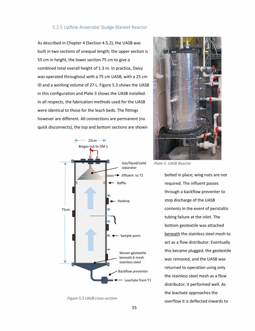
55
5.2.5 Upflow Anaerobic Sludge Blanket Reactor
As described in Chapter 4 (Section 4.5.2), the UASB was
built in two sections of unequal length; the upper section is
55 cm in height, the lower section 75 cm to give a
combined total overall height of 1.3 m. In practice, Daisy
was operated throughout with a 75 cm UASB, with a 25 cm
ID and a working volume of 27 L. Figure 5.3 shows the UASB
in this configuration and Plate 3 shows the UASB installed.
In all respects, the fabrication methods used for the UASB
were identical to those for the leach beds. The fittings
however are different. All connections are permanent (no
quick disconnects), the top and bottom sections are shown
bolted in place; wing nuts are not
required. The influent passes
through a backflow preventer to
stop discharge of the UASB
contents in the event of peristaltic
tubing failure at the inlet. The
bottom geotextile was attached
beneath the stainless steel mesh to
act as a flow distributor. Eventually
this became plugged, the geotextile
was removed, and the UASB was
returned to operation using only
the stainless steel mesh as a flow
distributor; it performed well. As
the leachate approaches the
overflow it is deflected inwards to
Plate 3. UASB Reactor
75cm
Backflow preventer
Baffle
Biogas out to GM 1
Leachate from T1
Woven geotextile beneath 6 mesh stainless-steel screen
Gas/liquid/solid separator
Effluent to T2
Heating
Sample ports
25cm
Figure 5.3 UASB cross-section

56
the gas liquid solid separator (GLS) by a baffle mounted on the wall. Inside the GLS, biogas bubbles
detach from the sludge granules and exit through the top, and thence to GM 1 (see Plate 1).
The particles descend back into the sludge bed and the liquid exits through the side of the reactor and
drains by gravity to T2; the system was constructed so that the effluent could be redirected to T1, but
Daisy was only operated this way to facilitate T2 removal for maintenance. The headspace above the
liquid in the UASB is separately vented to allow biogas
to exit through the top of the reactor and join the main
gas pipe; this prevents pressure buildup and hydraulic
disturbance in the UASB headspace above the GLS.
Five liquid/sludge sample ports were installed between
the inlet and the overflow. Heating tape was installed
along the length of the UASB. For clarity the RTD is
shown rotated 90° around the vertical axis from its
actual position. Plate 4 shows the finished heating tape
installation on the lower section of the UASB. Exactly
the same technique was used on the leach beds and on
the tanks. Each vessel was wrapped with 2 inch
aluminum tape. It covers the entire cylindrical surface
of the leach beds and UASB and all four sides of both
tanks to improve heat conduction across the surface of the vessels (the bottom of the tanks are
insulated with styrofoam). The heating tape was
also covered entirely with the aluminum tape to
hold it in place, ensure intimate contact with the
vessel wall and provide heat conduction from the
outside surface of the heating tape. Reflectix
insulation was then applied. There were fewer
constraints on the design of the UASB than on
that of the leach beds. As discussed in Section
4.5.2. by constructing the reactor in two sections,
and ensuring that the UASB feed pump had a
wide enough flow rate range, all practical
combinations of HRT and OLR and Vup could be
accomodated.
UASB effluent
Baffle
Biogas out
Figure 5.4 Schematic of GLS separator in UASB
Plate 4. Heating tape installation on UASB; sample points visible

57
The GLS separator was fabricated from a modified polypropylene funnel cemented into a female NPT
PVC fitting. The baffle located below the GLS is removable; it was constructed of two narrow sections of
25cm ID PVC pipe (2.5 cm and 1.0 cm in width respectively). Each has a section of its circumference
removed, such that it can be compressed and hold itself in place within the UASB like a piston ring. The
narrower section is installed within the wider section, to create a stepped profile (see Figure 5.4).
5.2.6 Leachate Tanks
The essential functions of leachate storage are set out in Section 4.5.3, including a total capacity of
around 40 L. In addition, one of the decisions from the lengthy deliberations about leach bed design
and function, was to include some form of clarifier ahead of the UASB, and to send the fines back to the
leach beds to filter them out (Section 5.2.4). The other constraint on the choices of tank configuration
*Can discharge to either tank
UASB FEED TANK LEACH BED FEED TANK
RTD
Clarifier To leach bed manifold
Return from leach bed manifold *UASB effluent
T1 – T2 exchange
T1 – T2 exchange
T1 – T2 balance
pipe
Sight glass (connected to gas system)
Biogas Biogas
Leachate drained from LBs
*UASB effluent
To UASB
Heating tape
RTD
Figure 5.5 Tanks 1 and 2
Plate 5. Tanks 1 and 2 plus Pumps 1, 2 and 3

58
was the matter of space; a single, low-profile, 40 L tank of appropriate dimensions was hard to find; I
also developed an operational preference for having two tanks to create some redundancy in the event
one had to be removed for service. The final choice was for two interconnected 20 L HDPE tanks, each
with a working volume of 17.5 L. Figure 5.5 shows Tanks 1 and 2 with their fittings and
interconnections. Plate 5 shows Tanks 1 and 2 plus the three pumps.
a) Design elements common to both tanks The tanks were identical when delivered. Each was modified to suit its specific purpose by cutting holes
and installing fittings as required. There were several common elements of design; both were fitted
with an RTD mounted through a bulkhead fitting in the roof of the tank. Both came equipped with a
large screw-on lid which was supposed to be gas tight. However, it proved hard to seal reliably. After
using silicone grease, then a gasket, then both (each of which worked for a while) I finally settled on
silicone sealant which was completely successful. More torque was required to remove the lid, and all
the old sealant had to be thoroughly removed, but this was an infrequent task and the inconvenience
was trivial.
Initially, a 100W immersion heater was installed through a bulkhead fitting in the lower side-wall of the
right-hand side of each tank. After about 30 days of operation, Tank 1 heater suffered a complete
failure. Suspended matter settled on the top of the heater element, lowering its efficiency and making
it work harder. Eventually silt, which had collected in the annulus between the heater element and the
bulkhead fitting, became baked in place by the overworking heater. This prevented any cooling of the
fitting, which promptly softened and began to leak. The system was shut down, the tanks removed, and
the immersion heaters replaced with heating tape. The heating tape was installed as described in
Section 5.2.5, and the tanks re-insulated. This design was much less responsive to demands for heat,
but more reliable and a lot safer. As part of the heater replacement modification, both tanks were
equipped with sight glasses to monitor liquid levels. The sight glasses are connected through lower
side-wall openings with bulkhead fittings on the right-hand side of each tank. At their open ends, the
sight glasses are connected to the gas manifold system to maintain hydraulic balance and prevent
blow-out. Biogas is vented through the top of both tanks to a joint manifold that, in turn, is connected
to the gas monitoring system.
Pump 2 (P2) transfers leachate at a low flow rate, between the two tanks, to help maintain hydraulic
balance. The initial plan was to install a level switch in T1 to turn P2 on and off as required. However, it
was feared that sludge would foul the level switch and compromise leachate flow to the UASB, so
instead a balance pipe was installed at the required leachate level of T1, permitting leachate levels to

59
equalize. Experience showed that operating with the flow from T2 to T1 at about 100 ml per minute
ensures that the clarifier never runs dry. Eventually this became standard operating practice. Once per
week however, all three pumps were run at full speed for 5 minutes to clear all the lines, flush the
piping, and reduce the buildup of solids. In the final step of this process, P2 is run at full speed in the
reverse direction, in an attempt to transfer accumulated solids from the bottom of T1 to T2 and from
there to the leach beds for filtration.
Both tanks have a roof-mounted aperture and valve for the purpose of introducing liquids. Most
commonly this was used to allow the addition of water to replace samples drawn from Daisy, and to
return the accumulated leachate that drained from fully digested leach beds after their removal from
the system.
a) Leach bed feed tank (Tank 1) As leachate drains from the six leach beds it flows into a common manifold that discharges into T1, near
the bottom right front. The conditions in T1 are fairly quiescent; under the operating conditions
adopted the T1 HRT is about 1.5 hours (depending on the T1/T2 exchange flowrate). The clarifier
consists of a section of 6 cm ID PVC pipe connected to a sump beneath T1. Clarified leachate is drawn
from the sump by P1 and delivered to the bottom of the UASB. Leachate is circulated between the two
tanks using a second transfer point located at the bottom left rear of T1. With the chosen leachate
recirculation rate through the leach beds, the flow rate of leachate draining to T1 exceeds the flowrate
to the UASB. This causes the level in T1 to rise, and the excess leachate to flow through the balance
P2
Tank 2
LB 2 LB 5 LB 6
LB 4
LB 3
UASB
Tank 1
P1
P3
7.2 l/h
6.0 l/h
30.6 l/h
1.1 l/h
LB 1
24.0 l/h
1.1 l/h 1.1 l/h 1.1 l/h 1.1 l/h 1.1 l/h
6.6 l/h
5.4 l/h 7.2 l/h
Figure 5.6 Leachate flows L/h - typical operating conditions

60
pipe to T2. The balance pipe is positioned to ensure that the leachate level in T1 is 2 cm higher than the
lip of the clarifier.
Tank 1 is also equipped with a return pipe for UASB effluent that discharges at the bottom right rear.
This was used only rarely to assist with maintenance.
b) Leach bed feed tank (Tank 2) Tank 2 serves as the reservoir from which the leach beds are fed. Pump 3 draws leachate from a
transfer point located at the bottom right front of the Tank and pumps it through a half inch pipe to the
leach bed manifold above LB1 on the left-hand side of Daisy. It flows through the manifold to the down-
comer on the right-hand side and back to T2 at the bottom right rear. The effluent from the UASB is
discharged to the bottom left rear of T2. The pickup point for leachate transfer to T1 is located left of
centre at mid-depth of the tank, and exits through a bulkhead fitting in the roof of the tank. Tank 2 also
receives overflow from T1, through the balance pipe, during periods of peak leachate drainage from the
leach beds. The combined flows of the entire system, from T2 through P3 back to T2, from T2 through
P3 and through the leach beds to T1, from T1 through P1 to the UASB to T2, from T2 through P2 to T1,
and the overflow from T1 to T2, are shown in Figure 5.6, a simplified schematic of liquid flows only.
5.2.7 Pumps and Valves
a) Pumps
Daisy is equipped with four identical peristaltic pumps, three active plus one spare. Flow requirements
were estimated (see Figure 5.6), and the pump specifications chosen such that the pumps would not be
required to run at more than about 60% of their rated maximum speed of 300 rpm. Norprene A-60-G
peristaltic tubing was chosen because of its long life. Published test data showed a mean time to failure
of 1000 hours at 600 RPM with a 3-roller pump head. In practice, and for greater safety and security,
the tubing was changed every 1000 hours but repositioned at 500 hours, and the maximum continuous
pump speed used was about 170 RPM. Three sizes of tubing were used; 1/8 ID, 3/16 inch ID, and 1/4 ID
for P1, P2 and P3 respectively. I experienced one pump head failure near the end of the experiment.
Daisy’s design also has built-in redundancy; it can operate for extended periods using P1 and P3 alone,
and for short periods with a single pump alternating between the duties of P1 and P3.
b) Valves Each leach bed was equipped with an automatic, pneumatically-actuated, three-way PVC valve (see
Figure 5.6). The leachate manifold comprises all 6 three-way valves connected in series; in the
normally-closed position the flow is straight through the valves, returning the leachate directly to T2. As

61
each valve is actuated in turn, the flow is redirected downward into the corresponding leach bed for a
predetermined time controlled by the PLC (see Section 5.2.9). Plate 6 shows 5 of the 6 valves with their
corresponding leach beds; the leach bed gas manifold is in the foreground.
There are, in total, 100 manual valves (including all shutoff valves and sampling points). They are
divided into 5 groups; quick disconnects, leachate, biogas, UASB, and pump; they are listed, coded, and
described in Appendix A. Every component is labelled to correspond to the equipment list. The quick
disconnects (VQ) are fitted only to the leach beds and are described in Section 5.2.4. The leachate
valves (VL) are primarily for the
purpose of taking samples, which can
be drawn from the outlet of each
leach bed and the outlet from both
tanks. They also have a secondary
purpose, allowing leachate flows to
be redirected with temporary tubing
for maintenance purposes, or to
permit occasional measurements of
Daisy’s behaviour, for example leach
bed permeability. The biogas valves (VG) allow gas flow from various components of the system to be
directed to one or other of the gas meters. Also, a tee-fitting with a butyl rubber septum in the side arm
was installed in the gas outlet from each leach bed, and the gas inlet to each gas meter, to permit the
withdrawal of biogas samples for GC analysis. The UASB valves (VU) permit sampling of the inflow of
leachate and the outflow of effluent and of the contents of the UASB (leachate and sludge) at different
depths within the reactor. Lastly, each pump is equipped with two valves (VP), one at the inlet and one
at the outlet, which can be closed to isolate the pumps for service or calibration.
All manual valves are made of PVC, the quick disconnects are made of PP, and all the interconnecting
piping and associated fittings are also made of PVC. The leachate drain lines are of 3/4 inch pipe, and
the leachate lines and the gas lines are of 1/2 inch pipe. All liquid lines, with the exception of the leach
bed drain lines, are insulated.
Plate 6. Leach beds, 3-way solenoid valves and leach bed gas manifold
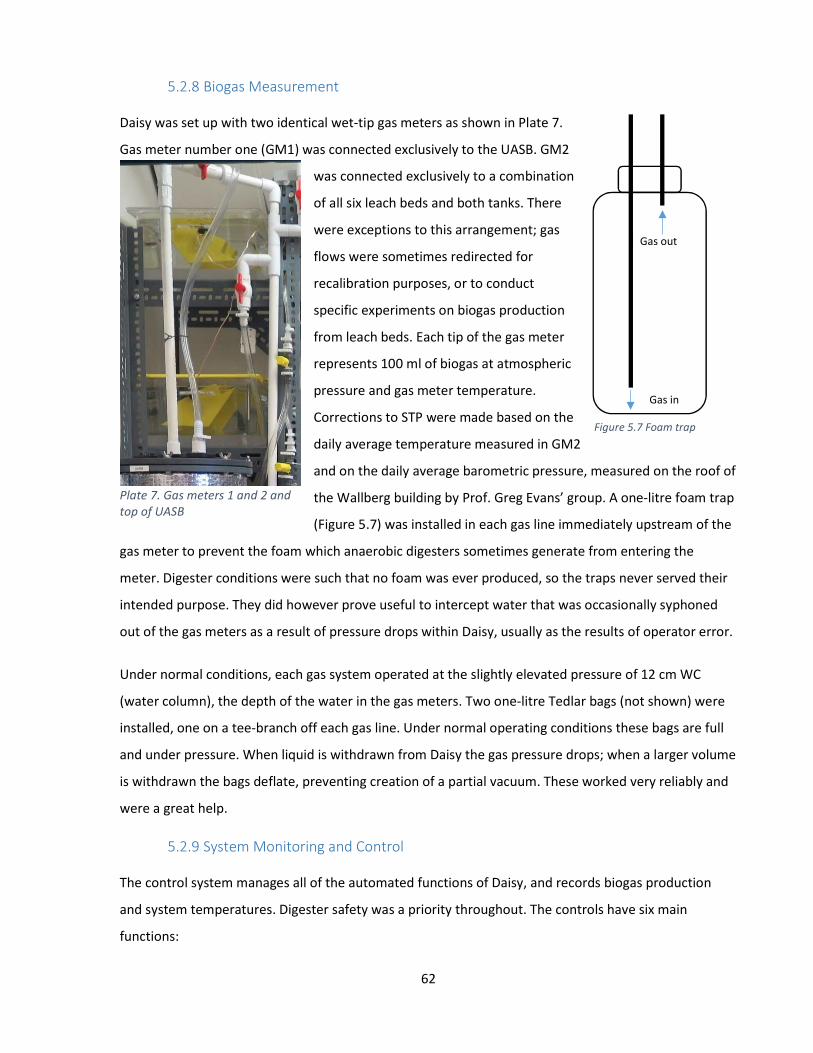
62
5.2.8 Biogas Measurement
Daisy was set up with two identical wet-tip gas meters as shown in Plate 7.
Gas meter number one (GM1) was connected exclusively to the UASB. GM2
was connected exclusively to a combination
of all six leach beds and both tanks. There
were exceptions to this arrangement; gas
flows were sometimes redirected for
recalibration purposes, or to conduct
specific experiments on biogas production
from leach beds. Each tip of the gas meter
represents 100 ml of biogas at atmospheric
pressure and gas meter temperature.
Corrections to STP were made based on the
daily average temperature measured in GM2
and on the daily average barometric pressure, measured on the roof of
the Wallberg building by Prof. Greg Evans’ group. A one-litre foam trap
(Figure 5.7) was installed in each gas line immediately upstream of the
gas meter to prevent the foam which anaerobic digesters sometimes generate from entering the
meter. Digester conditions were such that no foam was ever produced, so the traps never served their
intended purpose. They did however prove useful to intercept water that was occasionally syphoned
out of the gas meters as a result of pressure drops within Daisy, usually as the results of operator error.
Under normal conditions, each gas system operated at the slightly elevated pressure of 12 cm WC
(water column), the depth of the water in the gas meters. Two one-litre Tedlar bags (not shown) were
installed, one on a tee-branch off each gas line. Under normal operating conditions these bags are full
and under pressure. When liquid is withdrawn from Daisy the gas pressure drops; when a larger volume
is withdrawn the bags deflate, preventing creation of a partial vacuum. These worked very reliably and
were a great help.
5.2.9 System Monitoring and Control
The control system manages all of the automated functions of Daisy, and records biogas production
and system temperatures. Digester safety was a priority throughout. The controls have six main
functions:
Plate 7. Gas meters 1 and 2 and top of UASB
Gas out
Gas in
Figure 5.7 Foam trap

63
Valve sequencer – consisting of a PLC and six solenoid valves, each with a manual override
switch, the valve sequencer controls the opening and closing of the automated valves.
Signal transmitter - transmitter modules mounted in the transmitter rack to receive, process,
and distribute signals from the resistance temperature detectors (RTD) and the gas meters to
the data logger and to the temperature controllers.
Temperature controllers - three programmable temperature controllers, fed by a temperature
signal from the UASB and from each tank via the transmitter rack, activate solid-state relays to
deliver power to the heaters.
Data logger - the data logger records the tips of both gas meters and the temperatures from 10
different locations within Daisy.
E-stop - the Big Red Button permits emergency shutdown of the entire system. For added
safety, the power supply to the pumps, the leach bed heaters, and the air compressor are all
routed through the control panel, so that these components too are controlled by the E-Stop.
Internet connection – a specially assigned URL permits remote monitoring and downloading
from the data logger but, for security reasons, does not allow system control.
The following functions are manually controlled:
Pump speed and direction
Leach bed heaters
All other valves
Plate 8 shows the outside of the control panel during operation. Plate 9 shows the inside of the control
panel with all major components labelled.
a) Valve Sequencer and PLC The PLC controls the operation of the automatic valves, and the warning lights on the face of the
control panel display the system status (Plate 9). Pressing the START button activates the valve
sequencer which functions as follows:
on starting, there is a hold time (set as desired).
after the hold time expires, the first solenoid, for LB1, is energized and a dedicated timer is
started (time set as desired) .
when LB1 timer expires the LB1 solenoid is de-energized and its timer reset. There is a six
second delay (time set as desired) between the closure of LB1 solenoid and the opening of LB2
solenoid.
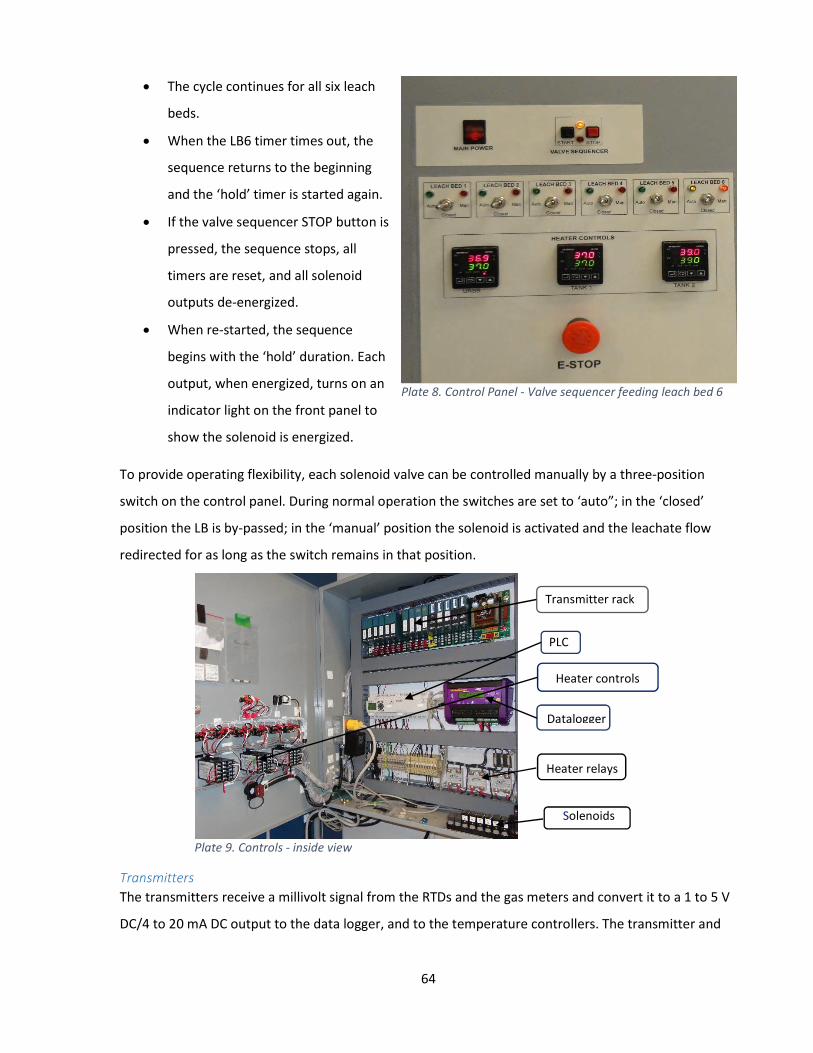
64
The cycle continues for all six leach
beds.
When the LB6 timer times out, the
sequence returns to the beginning
and the ‘hold’ timer is started again.
If the valve sequencer STOP button is
pressed, the sequence stops, all
timers are reset, and all solenoid
outputs de-energized.
When re-started, the sequence
begins with the ‘hold’ duration. Each
output, when energized, turns on an
indicator light on the front panel to
show the solenoid is energized.
To provide operating flexibility, each solenoid valve can be controlled manually by a three-position
switch on the control panel. During normal operation the switches are set to ‘auto”; in the ‘closed’
position the LB is by-passed; in the ‘manual’ position the solenoid is activated and the leachate flow
redirected for as long as the switch remains in that position.
Transmitters The transmitters receive a millivolt signal from the RTDs and the gas meters and convert it to a 1 to 5 V
DC/4 to 20 mA DC output to the data logger, and to the temperature controllers. The transmitter and
Heater relays
PLC
Heater controls
Datalogger
Plate 9. Controls - inside view
Solenoids
Transmitter rack
Plate 8. Control Panel - Valve sequencer feeding leach bed 6

65
transmitter rack are used components obtained by Glenn Wilson, free of charge, from Xerox
Corporation. The transmitters were modified with new resistors, and calibrated.
b) Temperature controllers Three automatic temperature controllers, one for each tank and one for the UASB, were installed in the
front of the control panel. Based on the RTD signals and the set-point, the controllers activate solid-
state relays which turn the power to the heaters on and off. The controllers themselves are
programmable; Initially they were set up using the ‘autotune’ feature that monitors the behaviour of
the temperatures being controlled and automatically sets the on-off cycle time and PID parameters
(proportional band, integral setting and the derivative or rate), then switches itself out of autotune.
Collectively these settings narrow the band within which the temperature fluctuates.
c) Data Logger The data logger was a dataTakr DT80 supplied by Dycor Technologies who also wrote the software for
this particular application and provided technical support free of charge. The system records
temperatures from 10 locations every 15 minutes, and gas meter tips every five minutes (plus hourly
totals) and stores all data in CSV format. Weijun Gao wrote a program to process downloaded data,
convert it to Excel format, and display the results in both tabular form, and graphically as follows;
Leach bed temperatures UASB, T1 and T2 temperatures GM2 temperature Hourly gas production – GM1, GM2 and total Cumulative gas production GM1, GM2 and total.
Downloading and conversion can be carried out for whatever periods of time one chooses, but was
always done daily. The Internet connection was used first thing every morning, to download results for
the previous 24 hours, examine them, link them to the daily log sheet and store them. Periodically, data
was also downloaded for more extended periods to view longer-term trends. The Internet connection
also provided the capability to monitor operations, which I did every morning and every night (and
often many times in between). With experience, it was possible to analyze and diagnose operating
anomalies very readily, usually from temperature patterns but also from gas measurements. On a
handful of occasions, this required a drive to the lab late at night to correct a problem. This obviated
much subsequent grief.
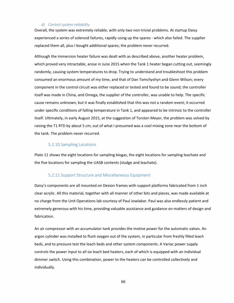
66
d) Control system reliability Overall, the system was extremely reliable, with only two non-trivial problems. At startup Daisy
experienced a series of solenoid failures, rapidly using up the spares - which also failed. The supplier
replaced them all, plus I bought additional spares; the problem never recurred.
Although the immersion heater failure was dealt with as described above, another heater problem,
which proved very intractable, arose in June 2015 when the Tank 1 heater began cutting out, seemingly
randomly, causing system temperatures to drop. Trying to understand and troubleshoot this problem
consumed an enormous amount of my time, and that of Dan Tomchyshyn and Glenn Wilson; every
component in the control circuit was either replaced or tested and found to be sound; the controller
itself was made in China, and Omega, the supplier of the controller, was unable to help. The specific
cause remains unknown, but it was finally established that this was not a random event; it occurred
under specific conditions of falling temperature in Tank 1, and appeared to be intrinsic to the controller
itself. Ultimately, in early August 2015, at the suggestion of Torsten Meyer, the problem was solved by
raising the T1 RTD by about 5 cm, out of what I presumed was a cool mixing zone near the bottom of
the tank. The problem never recurred.
5.2.10 Sampling Locations
Plate 11 shows the eight locations for sampling biogas, the eight locations for sampling leachate and
the five locations for sampling the UASB contents (sludge and leachate).
5.2.11 Support Structure and Miscellaneous Equipment
Daisy’s components are all mounted on Dexion frames with support platforms fabricated from 1 inch
clear acrylic. All this material, together with all manner of other bits and pieces, was made available at
no charge from the Unit Operations lab courtesy of Paul Jowlabar. Paul was also endlessly patient and
extremely generous with his time, providing valuable assistance and guidance on matters of design and
fabrication.
An air compressor with an accumulator tank provides the motive power for the automatic valves. An
argon cylinder was installed to flush oxygen out of the system, in particular from freshly filled leach
beds, and to pressure test the leach beds and other system components. A Variac power supply
controls the power input to all six leach bed heaters, each of which is equipped with an individual
dimmer switch. Using this combination, power to the heaters can be controlled collectively and
individually.
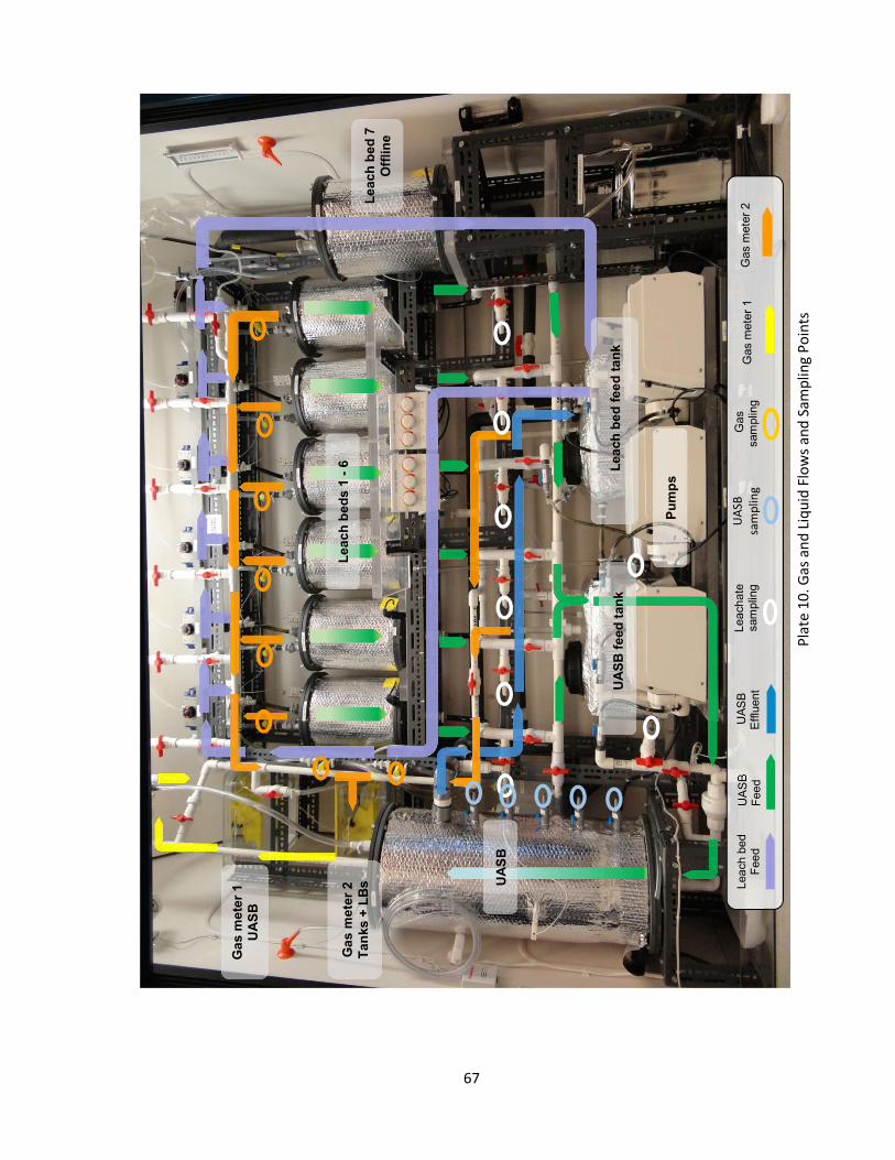
67
Pu
mp
s
UA
SB
fe
ed
ta
nk
L
ea
ch
be
d f
ee
d t
an
k
Ga
s m
ete
r 1
UA
SB
Ga
s m
ete
r 2
Ta
nk
s +
LB
s UA
SB
Le
ac
h b
ed
s 1
- 6
UA
SB
F
eed
Lea
ch b
ed
Fee
d
UA
SB
E
fflue
nt
Lea
chat
e
sam
plin
g G
as m
eter
1
Gas
met
er 2
G
as
sam
plin
g
Le
ac
h b
ed
7
Off
lin
e
Plat
e 10
. Gas
and
Liq
uid
Flow
s an
d Sa
mpl
ing
Poin
ts
UAS
B sa
mpl
ing
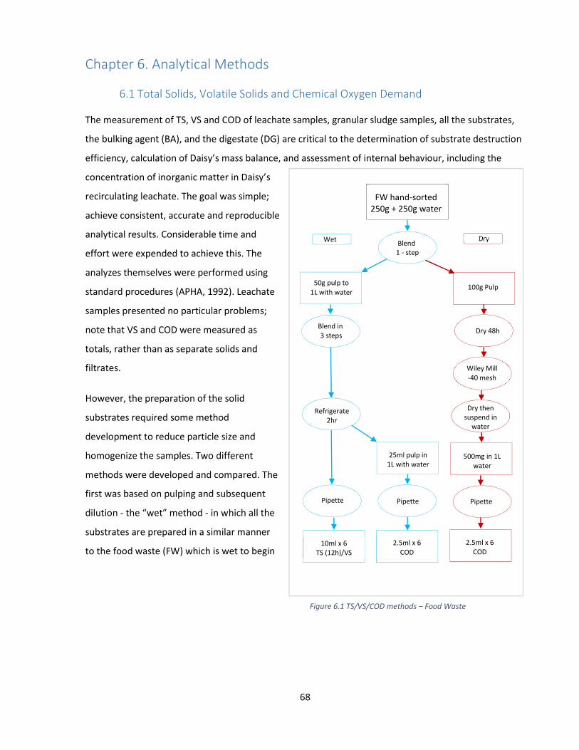
68
Chapter 6. Analytical Methods
6.1 Total Solids, Volatile Solids and Chemical Oxygen Demand
The measurement of TS, VS and COD of leachate samples, granular sludge samples, all the substrates,
the bulking agent (BA), and the digestate (DG) are critical to the determination of substrate destruction
efficiency, calculation of Daisy’s mass balance, and assessment of internal behaviour, including the
concentration of inorganic matter in Daisy’s
recirculating leachate. The goal was simple;
achieve consistent, accurate and reproducible
analytical results. Considerable time and
effort were expended to achieve this. The
analyzes themselves were performed using
standard procedures (APHA, 1992). Leachate
samples presented no particular problems;
note that VS and COD were measured as
totals, rather than as separate solids and
filtrates.
However, the preparation of the solid
substrates required some method
development to reduce particle size and
homogenize the samples. Two different
methods were developed and compared. The
first was based on pulping and subsequent
dilution - the “wet” method - in which all the
substrates are prepared in a similar manner
to the food waste (FW) which is wet to begin
Dry
Dry then suspend in
water
FW hand-sorted 250g + 250g water
DWet Blend 1 - step
50g pulp to 1L with water
Blend in 3 steps
Refrigerate 2hr
Pipette
10ml x 6 TS (12h)/VS
Pipette Pipette
2.5ml x 6 COD
2.5ml x 6 COD
100g Pulp
Dry 48h
Wiley Mill -40 mesh
25ml pulp in 1L with water
500mg in 1L water
Figure 6.1 TS/VS/COD methods – Food Waste
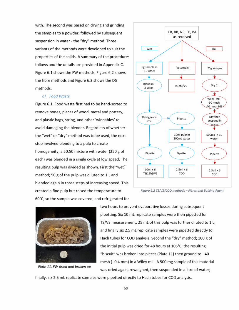
69
with. The second was based on drying and grinding
the samples to a powder, followed by subsequent
suspension in water - the “dry” method. Three
variants of the methods were developed to suit the
properties of the solids. A summary of the procedures
follows and the details are provided in Appendix C.
Figure 6.1 shows the FW methods, Figure 6.2 shows
the fibre methods and Figure 6.3 shows the DG
methods.
a) Food Waste
Figure 6.1. Food waste first had to be hand-sorted to
remove bones, pieces of wood, metal and pottery,
and plastic bags, string, and other ‘windables’ to
avoid damaging the blender. Regardless of whether
the “wet” or “dry” method was to be used, the next
step involved blending to a pulp to create
homogeneity; a 50:50 mixture with water (250 g of
each) was blended in a single cycle at low speed. The
resulting pulp was divided as shown. First the “wet”
method; 50 g of the pulp was diluted to 1 L and
blended again in three steps of increasing speed. This
created a fine pulp but raised the temperature to
60°C, so the sample was covered, and refrigerated for
two hours to prevent evaporative losses during subsequent
pipetting. Six 10 mL replicate samples were then pipetted for
TS/VS measurement; 25 mL of this pulp was further diluted to 1 L,
and finally six 2.5 mL replicate samples were pipetted directly to
Hach tubes for COD analysis. Second the “dry” method; 100 g of
the initial pulp was dried for 48 hours at 105°C; the resulting
“biscuit” was broken into pieces (Plate 11) then ground to - 40
mesh (- 0.4 mm) in a Wiley mill. A 500 mg sample of this material
was dried again, reweighed, then suspended in a litre of water;
finally, six 2.5 mL replicate samples were pipetted directly to Hach tubes for COD analysis.
Plate 11. FW dried and broken up
CB, BB, NP, FP, BA as-received
2.5ml x 6 COD
Dry then suspend in
water
500mg in 1L water
Pipette
D Wet Dry
6g sample in 1L water
Blend in 3 steps
Refrigerate 2hr
Pipette
10ml x 6 TS(12h)/VS
Pipette
2.5ml x 6 COD
25g sample
Dry 2h
Wiley Mill -60 mesh
-40 mesh NP
10ml pulp in 200mL water
4g sample
TS(2h)/VS
Pipette
Figure 6.2 TS/VS/COD methods – Fibres and Bulking Agent

70
b) Fibres Figure 6.2. No initial sorting was required
except for the removal of odd bits of plastic.
For the “wet” method, 6 g of dry sample were
blended in 1 L of water; the subsequent steps
were similar to those used for food waste. For
the dry method, triplicate samples of about 4 g
each (depending on the bulk density of the
fibre) were analyzed directly for TS and VS. A
25 g sample was dried for two hours then
ground in the Wiley mill to - 60 mesh
(-0.25 mm), except for NP to - 40 mesh (to
prevent screen plugging). These finely ground
samples were then suspended in water and
analyzed in the same way as the dried FW.
c) Digestate Figure 6.3. The samples have a high (78%)
moisture content. For the “wet” method, a 26g
sample of digestate was mixed in 1 L of water,
blended in three steps and then followed the
same steps as the fibres, with an additional
dilution step for the TS/VS samples. For the
“dry” method, the procedures are similar to
those for fibre samples, except that the initial
samples were of larger size because of their high moisture content, and their drying times
correspondingly longer.
d) Comparison of Methods Table 6.1 shows a comparison of COD measurements using both “wet” and “dry” methods; it also
includes published data and calculated values derived from elemental analyzes of three sets of milled
samples of substrates prepared using the “dry” method (see Section 6.2). The “wet” method gives
higher values than the “dry” method for all the substrates and for the DG; but for the BA the “dry”
method was slightly higher. The literature sources and the calculated values all confirm the accuracy of
the “dry” method, particularly for CB, BB and NP. The error analysis (± one STDEV) shows the “wet”
Dry D Wet
26g sample in 1L water
Blend in 3 steps
Refrigerate 2hr
Pipette
10ml x 6 TS(12h)/VS
Pipette
1.5ml x 6 COD
25g sample
10ml pulp in 200mL water
20g sample
Pipette
Digestate as-sampled
25ml pulp in 500mL water
Pipette
TS(48h)/VS Dry 48h
Pipette
1.5ml x 6 COD
Wiley Mill -40 mesh
Dry then Suspend in
water
500mg in 1L water
Figure 6.3 TS/VS/COD methods - Digestate

71
method to be less precise. The potential for errors in the “wet” method could be observed in the
numerous pipetting steps required. Despite all the energy input from the blender, larger particles were
still present and could be seen during pipetting; occasional plugging of the cut-tip pipette was
unavoidable. In all respects, the “dry” method proved simpler, and less subject to random error.
Table 6.1 Comparison of COD Analysis Methods COD g/gTS
Sample Calculated from Elemental Analysis Literature Measured 1 2 3 Avg. STDEV Dry1 Dry2 STDEV Dry Error Wet STDEV
Cardboard (CB) 1.16 1.14 1.10 1.13 0.03 1.08 1.10 0.02 1.14 0.05 1.33 0.12
Boxboard (BB) 1.12 1.08 1.09 1.10 0.02 1.12 - - 1.13 0.01 1.28 0.12
Newsprint (NP) 1.34 1.28 1.27 1.30 0.04 1.22 1.21 0.03 1.33 0.02 1.43 0.15
Fine paper (FP) 1.09 1.03 1.05 1.05 0.03 1.07 1.07 0.02 1.00 0.03 1.05 0.15
Food waste (FW) 1.53 1.38 1.48 1.46 0.07 - - 1.30 0.11 1.37 0.12
Bulking agent (BA) 1.27 1.26 1.31 1.28 0.02 - - 1.32 0.05 1.27 0.14
Digestate (DG)
1.19 0.05 1.21 0.10
The data presented here represent the analysis of a large number of samples over a period of many
months, and led to the conclusion that the dry method was preferred for the reasons outlined.
Ultimately this conclusion was confirmed by the mass balance calculations presented later. However, I
was not able to determine the cause of the systematically higher results obtained using the “wet”
method, other than to say that it is highly unlikely that pipetting errors could have created the
systematic errors observed. All of the results presented in this thesis are based upon data obtained
using the “dry” method (unless otherwise noted).
e) Digestion of individual substrates – using coupons While it was possible to measure the
TS/VS/COD content of the individual
substrates going in, it was impossible
to separate them, or form any
opinion about their digestibility on
the way out; only the overall
digestibility of the aggregate waste
mass could be determined. To
remedy this a very simple analytical
procedure, the coupon method, was
developed. Each leach bed of fresh
waste received stainless steel tea
1(Pommier et al., 2010) 2(Yuan et al., 2014)
Plate 12. Installing triplicate coupons for digestibility determination

72
balls (coupons) containing samples of individual substrates or bulking agent on a rotating schedule
summarized in Table 6.2. Two sets of three 2.5 cm tea balls, each set comprising triplicate weighed
quantities of one specific substrate, were inserted
into the first, second, fourth and fifth leach beds in
a six-week sequence. For example, in Week 2 three
coupons of BB were placed at a depth of 25 cm and
three coupons of FP at a depth of 20 cm (see Plate
12). In weeks three and six a single 5 cm coupon,
filled with BA, was placed in the middle of the leach
bed. The larger size was necessary because the low digestibility of the wood chips required larger
samples and BA consists of relatively large particles. Installing three of these in a single leach bed would
have taken up too much space and disrupted hydraulic flow patterns. The bottom half of the BA
coupons was lined with a glass fibre filter paper to retain fines and prevent false results.
In this manner the contents of each coupon were exposed to the same digestion conditions as the rest
of the feedstock, but kept separate from it, enabling individual destruction efficiencies to be measured.
Another advantage of this procedure was that the substrates were being digested in exactly the same
form as they were present in the bulk mass of waste; that is without any further size reduction.
At the end of the digestion period, the coupons were carefully removed, weighed wet, dried and TS
measured. To measure VS, it was necessary to remove the dried digested material from the coupon and
re-weigh it into an aluminum dish. Repeated trips to the furnace at 550° C would soon have destroyed
the tea balls. Attempts were made to find materials other than stainless steel tea balls for use as
coupons to minimize flow anomalies; for example durable fabrics, whose shape would conform to the
waste as it was digested. However, none could be found that would function as required, and survive
the trip through the drying oven.
6.2 Elemental Analysis
Three complete sets of samples, each comprising CB, BB, NP, FP, BA, FW, and DG, were analyzed for C,
H, and N content. The analyzes were performed by ANALEST, a commercial lab in the Department of
Chemistry.
The equipment used was a Thermo Flash 2000 CHN Analyzer, which is based on the principle of
dynamic flash combustion, and uses a single reaction tube (combustion and reduction function
combined). Grade 5.0 He is the carrier, with a flow rate of 140 mL/min.
Table 6.2 Coupon Placement in Leach Beds Week Size Coupon Depth
25 cm 20 cm 1 2.5 cm CB NP 2 2.5 cm BB FP 3 5.0 cm BA
4 2.5 cm NP CB 5 2.5 cm FP BB 6 5.0 cm BA
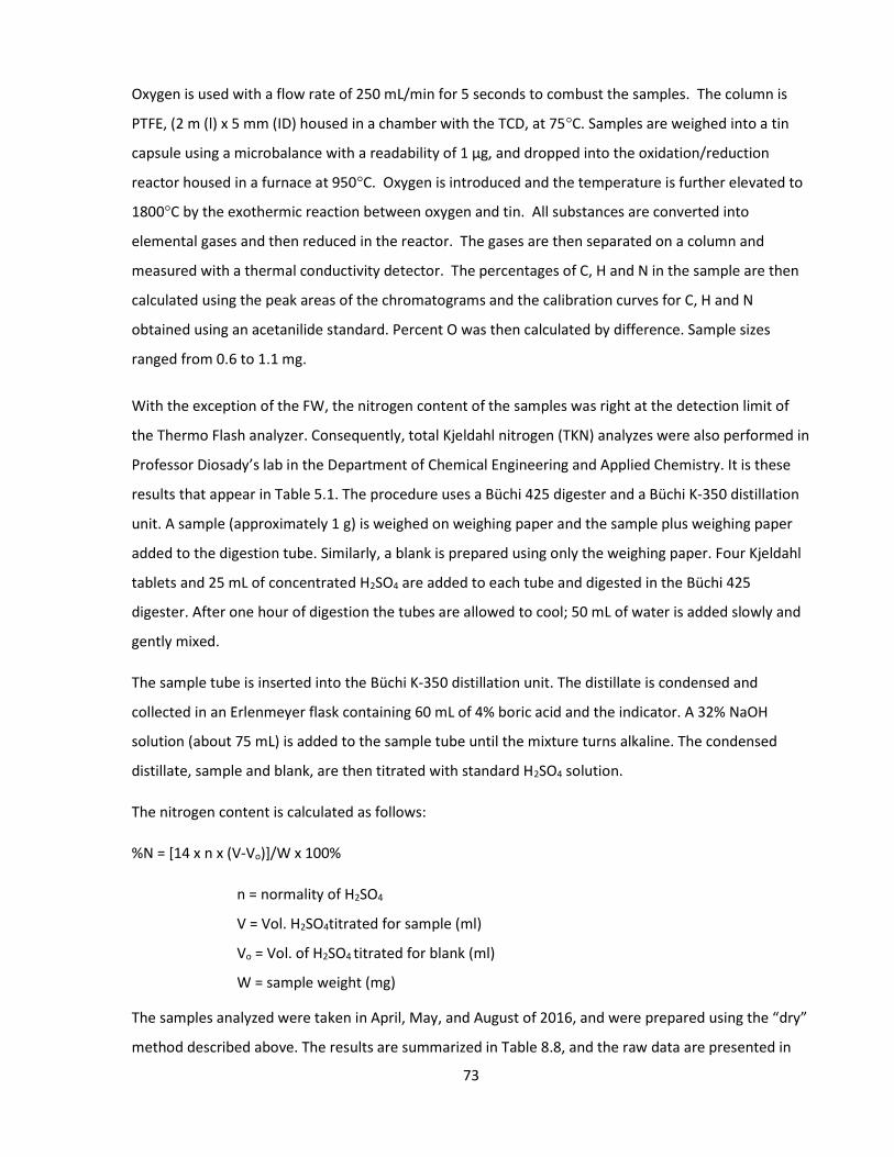
73
Oxygen is used with a flow rate of 250 mL/min for 5 seconds to combust the samples. The column is
PTFE, (2 m (l) x 5 mm (ID) housed in a chamber with the TCD, at 75°C. Samples are weighed into a tin
capsule using a microbalance with a readability of 1 µg, and dropped into the oxidation/reduction
reactor housed in a furnace at 950°C. Oxygen is introduced and the temperature is further elevated to
1800°C by the exothermic reaction between oxygen and tin. All substances are converted into
elemental gases and then reduced in the reactor. The gases are then separated on a column and
measured with a thermal conductivity detector. The percentages of C, H and N in the sample are then
calculated using the peak areas of the chromatograms and the calibration curves for C, H and N
obtained using an acetanilide standard. Percent O was then calculated by difference. Sample sizes
ranged from 0.6 to 1.1 mg.
With the exception of the FW, the nitrogen content of the samples was right at the detection limit of
the Thermo Flash analyzer. Consequently, total Kjeldahl nitrogen (TKN) analyzes were also performed in
Professor Diosady’s lab in the Department of Chemical Engineering and Applied Chemistry. It is these
results that appear in Table 5.1. The procedure uses a Büchi 425 digester and a Büchi K-350 distillation
unit. A sample (approximately 1 g) is weighed on weighing paper and the sample plus weighing paper
added to the digestion tube. Similarly, a blank is prepared using only the weighing paper. Four Kjeldahl
tablets and 25 mL of concentrated H2SO4 are added to each tube and digested in the Büchi 425
digester. After one hour of digestion the tubes are allowed to cool; 50 mL of water is added slowly and
gently mixed.
The sample tube is inserted into the Büchi K-350 distillation unit. The distillate is condensed and
collected in an Erlenmeyer flask containing 60 mL of 4% boric acid and the indicator. A 32% NaOH
solution (about 75 mL) is added to the sample tube until the mixture turns alkaline. The condensed
distillate, sample and blank, are then titrated with standard H2SO4 solution.
The nitrogen content is calculated as follows:
%N = [14 x n x (V-Vo)]/W x 100%
n = normality of H2SO4
V = Vol. H2SO4titrated for sample (ml)
Vo = Vol. of H2SO4 titrated for blank (ml)
W = sample weight (mg)
The samples analyzed were taken in April, May, and August of 2016, and were prepared using the “dry”
method described above. The results are summarized in Table 8.8, and the raw data are presented in

74
Appendix C. They are remarkable for their consistency; the greatest variability is seen in the FW, which
is intrinsic to the material itself and to be expected. Each analysis, using both methods, was carried out
in duplicate.
6.3 Volatile Fatty Acids and Sulphate
VFAs and sulphate were analyzed using a Dionex ICS-2100 ion chromatograph. The column was an RFIC
Ionpac with an AG18 guard column/AS18 analytical column. The runtime was 23 minutes per sample.
The eluent was a KOH solution at a flow rate of 1 mL/min. Using the gradient method, the eluent
concentration was increased from 2 mM to 32 mM over the first 15 minutes, and remained at 32 mM
for 3 min then reduced to 2mM for the remaining 5 min. Suppressor values were 80 mA. Standards
were prepared at 5, 10, 50, 100, 200, and 500 µM, by making serial dilutions of 10 mM solutions of
sodium acetate sodium propionate and sodium butyrate, with 18 MΩ Milli-Q water.
Leachate samples (10 mL) were taken from Daisy (contemporaneously with separate samples obtained
for analysis of TS, VS and COD, and pH and alkalinity) and immediately filtered with a 0.22 µm syringe
filter, and stored at -20° C. After initial trials, samples were diluted 5X, 10X, 20 X, and 50X as required,
to fall within the calibration range. A six point calibration was included in every run; two blanks were
run prior to and following each set of standard samples. The concentration of each VFA and of sulphate
was calculated in µM, by the software in instrument, using the calibration data from the run.
All of the VFA and sulphate analyses were performed by Masters student Peter HyunWoo Lee (thank
you Peter).
6.4 Alkalinity and pH
Leachate samples were analyzed regularly for pH and alkalinity ratio. The latter is calculated as the ratio
of intermediate alkalinity (IA) to partial alkalinity (PA). Two methods were compared during start up
with synthetic feed (see Chapter 7 Section 7.3.2). The method of Ripley et al. (1986) is based on a two-
step titration; step 1
from starting pH to
pH 5.75, and step 2
from pH 5.75 to pH
4.3. The second
method, of uncertain origin but believed to come from the USEPA, is based on a titration from starting
pH to pH 4.0, followed by boiling to evaporate VFAs, then a back-titration to pH 7.0. Each method was
Table 6.3 – Synthetic Feed - pH and Alkalinity Day 56 pH PA IA IA/PA
USEPA fresh sample 7.01 1330 360 0.32 USEPA centrif. Sample 7.32 1220 510 0.44 Ripley fresh sample 7.01 1110 510 0.46 Ripley centrif. Sample 7.32 1190 470 0.39

75
tested on raw leachate and centrifuged leachate. In both methods titration was carried out with 0.1N
H2SO4 using a pH meter. The results, comparing both methods, are shown in Table 6.3.
The Ripley method is much less involved, did not give materially different results, and so became the
method of choice for all subsequent tests (without filtration or centrifugation of the sample). According
to Ripley, the ideal range for stable operation is an alkalinity ratio < 0.5 and preferably <0.4. The
usefulness of this method was demonstrated by Zhang et al. (2013); the IA/PA started to rise ̴20d
before the pH started to fall leading to reactor failure.
6.5 Biogas Analysis
Samples of biogas were analyzed using a Hewlett Packard 5890 equipped with CTR I column and a
thermal conductivity detector (TCD). Helium was used as the carrier gas at a column pressure of 180
kPa. The injector and detector were both set at 200˚C. The oven temperature was operated
isothermally at 50˚C and the runtime was set at 11 minutes. Methane and CO2 standards were used to
prepare calibration curves. Serum bottles were filled with high-purity standard gases by bubbling on the
water; the bottles were closed with butyl stoppers; the calibration curves were created by withdrawing
five aliquots of standard gas, 200 µL, 150 µL, 100 µL, 50 µL, and 25 µL, and injecting them into the GC.
CO2 was eluted at about 0.45 min. and methane was eluted at about 8 min. The results were used to
generate a calibration curve for each gas. The GC was calibrated three times during the course of the
research programme.
Samples of biogas, 200 μL, were extracted from Daisy using a 500 μL gas-tight syringe, and injected into
the GC. The CH4 and CO2 content were determined from the slope of the calibration curves.
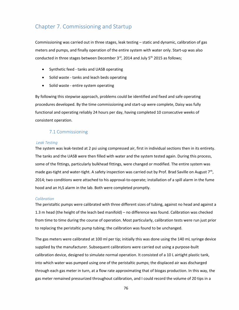
76
Chapter 7. Commissioning and Startup
Commissioning was carried out in three stages, leak testing – static and dynamic, calibration of gas
meters and pumps, and finally operation of the entire system with water only. Start-up was also
conducted in three stages between December 3rd, 2014 and July 5th 2015 as follows;
Synthetic feed - tanks and UASB operating
Solid waste - tanks and leach beds operating
Solid waste - entire system operating
By following this stepwise approach, problems could be identified and fixed and safe operating
procedures developed. By the time commissioning and start-up were complete, Daisy was fully
functional and operating reliably 24 hours per day, having completed 10 consecutive weeks of
consistent operation.
7.1 Commissioning
Leak Testing The system was leak-tested at 2 psi using compressed air, first in individual sections then in its entirety.
The tanks and the UASB were then filled with water and the system tested again. During this process,
some of the fittings, particularly bulkhead fittings, were changed or modified. The entire system was
made gas-tight and water-tight. A safety inspection was carried out by Prof. Brad Saville on August 7th,
2014; two conditions were attached to his approval-to-operate; installation of a spill alarm in the fume
hood and an H2S alarm in the lab. Both were completed promptly.
Calibration The peristaltic pumps were calibrated with three different sizes of tubing, against no head and against a
1.3 m head (the height of the leach bed manifold) – no difference was found. Calibration was checked
from time to time during the course of operation. Most particularly, calibration tests were run just prior
to replacing the peristaltic pump tubing; the calibration was found to be unchanged.
The gas meters were calibrated at 100 ml per tip; initially this was done using the 140 mL syringe device
supplied by the manufacturer. Subsequent calibrations were carried out using a purpose-built
calibration device, designed to simulate normal operation. It consisted of a 10 L airtight plastic tank,
into which water was pumped using one of the peristaltic pumps; the displaced air was discharged
through each gas meter in turn, at a flow rate approximating that of biogas production. In this way, the
gas meter remained pressurized throughout calibration, and I could record the volume of 20 tips in a
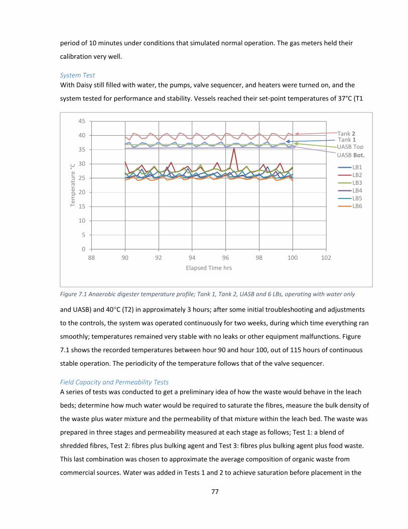
77
period of 10 minutes under conditions that simulated normal operation. The gas meters held their
calibration very well.
System Test With Daisy still filled with water, the pumps, valve sequencer, and heaters were turned on, and the
system tested for performance and stability. Vessels reached their set-point temperatures of 37°C (T1
and UASB) and 40°C (T2) in approximately 3 hours; after some initial troubleshooting and adjustments
to the controls, the system was operated continuously for two weeks, during which time everything ran
smoothly; temperatures remained very stable with no leaks or other equipment malfunctions. Figure
7.1 shows the recorded temperatures between hour 90 and hour 100, out of 115 hours of continuous
stable operation. The periodicity of the temperature follows that of the valve sequencer.
Field Capacity and Permeability Tests A series of tests was conducted to get a preliminary idea of how the waste would behave in the leach
beds; determine how much water would be required to saturate the fibres, measure the bulk density of
the waste plus water mixture and the permeability of that mixture within the leach bed. The waste was
prepared in three stages and permeability measured at each stage as follows; Test 1: a blend of
shredded fibres, Test 2: fibres plus bulking agent and Test 3: fibres plus bulking agent plus food waste.
This last combination was chosen to approximate the average composition of organic waste from
commercial sources. Water was added in Tests 1 and 2 to achieve saturation before placement in the
0
5
10
15
20
25
30
35
40
45
88 90 92 94 96 98 100 102
Tem
pera
ture
°C
Elapsed Time hrs
LB1LB2LB3LB4LB5LB6
Tank 2Tank 1UASB TopUASB Bot.
Figure 7.1 Anaerobic digester temperature profile; Tank 1, Tank 2, UASB and 6 LBs, operating with water only

78
leach beds. Test 3 was a continuation of Test 2, with food waste added. The frozen food waste released
some free water when thawed, so no further water was added to the waste in Test 3. The prepared
waste was placed in a single leach bed, lightly packed down, and the headspace above the waste
measured. Two paper towels (unbleached paper) were placed on top of the waste, followed by a disc of
non-woven geotextile, equal in diameter to the leach bed. The purpose of this combination was to
disperse the added leachate across the top of the waste before it drained into, and through, the waste.
The paper towels were not used after this first trial. The leach bed was then closed, weighed, installed,
and allowed to drain for one hour to release any surplus water; the drained water was measured, and
subtracted from the water added, to calculate the saturation capacity of the waste. Water (535 ml) was
then introduced into the leach bed by setting the three-way valve to “Manual” for one minute; the
volume collected at the bottom of the leach bed was measured at intervals. At the conclusion of the
tests, the waste was allowed to drain for 24 hours, the leach bed weighed again, the headspace
measured, and the total weight and density of saturated waste determined. The waste composition is
shown in Table 7.1 and the results of the permeability tests in Figure 7.2. No settlement of the waste
was observed.
Several observations were made and conclusions drawn. The fibres and woodchips require a lot of
water to reach saturation, and this must be added before the waste is introduced to the digester – both
to ensure proper mixing, and to avoid
excessive drawdown of the leachate in
Tank 2. Assuming that the food waste is
about 70% moisture (a good figure
from the literature), the final moisture
content of the waste mixture was 72%,
66% and 68% in Tests 1, 2 and 3
respectively. This indicated that, for a
solids retention time of 42 days, about
3.7 litres of free water per week would be generated, and require removal from the system but, in
practice, none was. The permeability tests show that fibre alone drained very rapidly, and all the added
water was drained within 60 minutes; fibre plus woodchips had a lower initial permeability but still
drained all the water within 70 minutes; the addition of food waste flattened the curve further, and at
60 minutes the waste still retained 28% of the added water. Nevertheless, twenty four hours later, all
the water had drained (not shown). This prolonged retention of water was thought to be favourable for
Table 7.1 Permeability Tests Test 1 Test 2 Test 3
Newsprint 0.10 kg 0.10 kg 0.10 kg Cardboard 0.44 kg 0.44 kg 0.44 kg Boxboard 0.35 kg 0.35 kg 0.35 kg Fine paper 0.20 kg 0.20 kg 0.20 kg Woodchips
0.50 kg 0.50 kg
Food waste
0.73 kg Water added 2.74 kg 3.17 kg 3.07 kg Total mass 3.83 kg 4.76 kg 5.29 kg
Volume 5.65 l 7.70 l 8.48 l Density 0.68 kg/l 0.62 kg/l 0.62 kg/l

79
hydrolysis, but there remained a concern about how the permeability might change as digestion
progressed, and how effective the bulking agent would be.
Summary (Commissioning) All the sub-systems and the digester as a whole were made leak-free with both air and water
under conditions of elevated pressure. The peristaltic pumps and the gas meters were successfully calibrated. The system as a whole was filled with water, brought to operating temperature, and run for
115 hours without incident. The permeability of the proposed mixture of substrates and bulking agent was tested and
found to have a beneficial effect by slowing initial leachate flow and slightly delaying drainage, both helpful for leachate substrate contact.
7.2 Startup of Daisy with Synthetic Feed - Tanks and UASB operating
The first stage of startup was carried out with a synthetic feed, using the tanks and UASB only, with the
leach beds empty but the valve sequencer operating, so the leachate flowed through the leach beds
directly to Tank 1. The inoculum in the UASB consisted of sludge from Maryland Farms (MF), an on-farm
digester in Ontario, licensed to process food waste from commercial sources but only processing farm
waste at the time the samples were taken. Daisy was operated in this mode continuously for 59 days.
Biogas composition was measured and BMP tests were run. She was then decommissioned, cleaned,
and thoroughly leak-tested. The general conclusion from this phase was that all the components of the
system performed more or less as planned and that startup with synthetic feed could begin.
0
100
200
300
400
500
600
0 20 40 60 80
Leac
hate
dra
ined
mL
Elapsed time min.
Fibre + woodchips
Fibre + woodchips + food waste
Fibre alone
Figure 7.2 Waste permeability tests; FB alone, FB+BA, FB+BA+FW
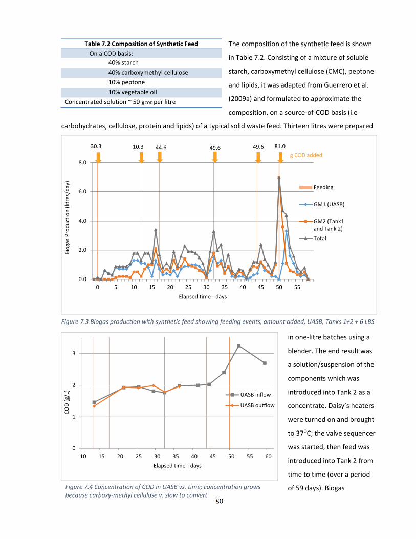
80
The composition of the synthetic feed is shown
in Table 7.2. Consisting of a mixture of soluble
starch, carboxymethyl cellulose (CMC), peptone
and lipids, it was adapted from Guerrero et al.
(2009a) and formulated to approximate the
composition, on a source-of-COD basis (i.e
carbohydrates, cellulose, protein and lipids) of a typical solid waste feed. Thirteen litres were prepared
in one-litre batches using a
blender. The end result was
a solution/suspension of the
components which was
introduced into Tank 2 as a
concentrate. Daisy’s heaters
were turned on and brought
to 37OC; the valve sequencer
was started, then feed was
introduced into Tank 2 from
time to time (over a period
of 59 days). Biogas
Table 7.2 Composition of Synthetic Feed On a COD basis:
40% starch 40% carboxymethyl cellulose 10% peptone 10% vegetable oil
Concentrated solution ~ 50 gCOD per litre
0.0
2.0
4.0
6.0
8.0
0 5 10 15 20 25 30 35 40 45 50 55
Biog
as P
rodu
ctio
n (li
tres
/day
)
Elapsed time - days
Feeding
GM1 (UASB)
GM2 (Tank1and Tank 2)
Total
g COD added44.630.3 10.3 49.6 49.6 81.0
Figure 7.3 Biogas production with synthetic feed showing feeding events, amount added, UASB, Tanks 1+2 + 6 LBS
0
1
2
3
10 15 20 25 30 35 40 45 50 55 60
COD
(g/L
)
Elapsed time - days
UASB inflow
UASB outflow
Figure 7.4 Concentration of COD in UASB vs. time; concentration grows because carboxy-methyl cellulose v. slow to convert

81
production was recorded. Samples of leachate were taken at intervals of 3 to 5 days and analyzed for
TS/VS/COD using standard methods. Towards the end of the trial period, samples of leachate were
analyzed for pH and alkalinity for the purposes of method comparison (see Table 6.3). Biogas was
sampled at each gas meter and its composition analyzed using GC-TCD. Four litres of MF sludge at 72
gCOD.L-1, was introduced to the UASB.
Biogas production for the entire 59 day period is shown in Fig. 7.3 which also shows how much feed
was added and when. The COD concentration in the leachate for the same period is presented in Fig.
7.4 and shows a rise in COD concentration to a plateau, then another rise throughout the test period.
The total biogas yield was 84.9L at 53.2% CH4 and 297K.
A BMP test (BMP 1) was performed in triplicate on six samples and two controls; each of the four
synthetic feed components, plus the whole feed, were tested with MF sludge, and the whole feed
tested with an alternative inoculum, Tembec granules, from an anaerobic digester treating pulp mill
effluents located at Temiskaming. The details of this test are provided in Appendix E.
Two principal conclusions were drawn from Daisy’s operating data; addition of fresh feed created an
immediate spike in biogas production which quickly subsided, and the amount of gas produced was less
than would be expected if most of the feed added had been consumed. It is believed that the starch
was being rapidly consumed but that the CMC was, for reasons unknown, not being digested, leading to
the steady rise in COD concentration. The results of the BMP test (Figure 7.5) confirmed this conclusion,
showing that even after 65 days only 23% of the CMC was digested but 95% of the starch and 86% of
0.0
10.0
20.0
30.0
40.0
50.0
60.0
70.0
80.0
90.0
0 10 20 30 40 50 60 70
Biog
as p
rodu
ced
mL
(at 2
97K)
Elapsed Time - days
Tembec + SF
MF sludge +SF
MF sludge +starchMF sludge +CMCMF sludge +peptoneMF sludge +lipidsTembec
MF sludge
Max.
Figure 7.5 Synthetic feed BMP results. Tembec granules + SF; MF sludge +SF, +starch, +CMC, +peptone, +lipids. Tembec granules alone, MF sludge alone.

82
the peptone had been digested (based on the theoretical maximum biogas production of 76 mL for all
samples). The MF sludge showed lag times of 10 to 20 days, depending on the substrate. The Tembec
granules showed no lag time, a much higher initial rate, and a more typical curve.
Summary (Start-up, synthetic feed) Tembec granules are a superior inoculum to Maryland Farms sludge. Ripley’s procedure is the preferred method for measuring alkalinity. GC-TCD worked well for biogas analysis. The synthetic feed was suitable for the purposes of initial start-up. Datalogging of temperatures and gas production was reliable. Daisy performed as planned, all system components functioned well and no operating
problems were experienced.
7.3 Startup of Daisy - Tanks and Leach Beds operating
To start up the leach beds, three were charged simultaneously with a mixture of FW, FB, and BA plus 90
g of Tembec granules in each leach bed as inoculum. The feedstock composition is shown in Table 7.3.
This mixture approximates the average composition of commercial organic waste in the City of Ottawa
(MacViro Consultants, 2007). The amount of water added, comprising 62.6% of the total, is typical of
“field capacity” (saturation) of solid waste within a landfill. The food waste came from the green bin
program operated by Miller Waste Systems for the Region of Durham and during the course of the
research programme Miller delivered two shipments. Both were collected early in the month of May;
the date was chosen so that it was warm enough to successfully sort, coarsely shred (shear shredder
with 4 inch knives) and repackage the bulk material, but cool enough to minimize premature
degradation. The food waste was stored at -20°C. The fibres and bulking agent were also supplied by
Miller; they came from the York Region Materials Recovery Facility operated by Miller. Lastly, the
bulking agent was ash wood ground by Miller using a commercial Roto-Chopper.
Table 7.3 – Composition of Digester Feedstock per Leach Bed– Period 1
Category Component Code Quantity g. Percent of TS Percent of VS Percent of COD Fibre Cardboard CB 440 33.0 33.5 32.5 Boxboard BB 350 28.1 27.3 27.5 Newsprint NP 110 8.3 9.2 9.6 Fine paper FP 200 15.3 14.5 13.2 Sub-total fibre FB 1,100 Food waste Green bin waste FW 675 15.3 15.4 17.2 Bulking agent Ash wood chips BA 500 Water 3,800 Total 6,075
83
All three leach beds were started simultaneously on February 17th 2015 (the UASB was idle); since
inoculum had been added to each leach bed, biogas production began quickly, but also ended very
quickly. By February 20th all biogas production had ceased. By February 24th the alkalinity ratio had risen
to 3.29 and the pH had dropped to 5.5. Sodium bicarbonate addition returned the pH to 6.90 but the
alkalinity ratio remained very high at 2.14 indicating incipient reactor failure. The system had essentially
failed because of a lack of inoculum; it is believed that Daisy was either producing fatty acids far more
quickly than she could consume them, or the food waste contained more soluble COD than the
inoculum could convert. At this point the immersion heater in Tank 2 suffered a progressive failure as a
result of fouling; the system was immediately shut down for repair. External heat tapes were installed
in place of immersion heaters; these were tested with water in the system and found to be satisfactory;
the rate of heating was significantly lower than with the immersion heaters but, since the objective is
temperature stability within a narrow range, this was of no concern. More details can be found in
Section 5.1.3. The modifications took four weeks to complete. During the shut-down the waste was left
sealed in leach beds 1, 2 and 3.
Summary (Start-up, solid waste) The alkalinity ratio responded to the process upset as intended, but under the prevailing
conditions and given the trial and error nature of the operation at this stage, there was no feasible way to prevent reactor failure.
The leach beds worked well, in that the recirculating leachate led to hydrolysis of the feed and a build-up of soluble/suspended COD in the system.
Direct heating does not work in this environment because suspended particulate matter leads to fouling of the heater elements and failure of the bulkhead fitting.
7.4 Startup of Daisy – Entire System operating
This phase of the start-up process ran from March 23, 2015 to July 5, 2015 (104 days) and was carried
out with ten specific objectives:
1. Test each component of the system under typical operating conditions for an extended
period
2. Test the system as a whole
3. Establish feeding protocols
4. Establish digestate removal and sampling protocols
5. Establish sampling and analytical procedures; location, sample size and frequency
6. Identify and correct any defects
7. Learn the interrelationships among variables

84
8. Refine operating practices
9. Gather as much data as possible, and complete a preliminary assessment of performance
10. Establish a baseline of digester performance from which to plan and conduct the balance of
the research programme.
Process operation – Period 1 The original three leach beds, designated S.001, S.002 and S.003 (all the leach beds were numbered
sequentially in this manner) were reactivated on March 23, 2015 (Day 0) after a 28 day hiatus. Details
of the contents and history of S.001 to S.087 can be found in EDF5. The leachate, which had been
stored at 4°C during the shut-down, was returned to the Tanks and brought to operating temperature.
The headspace of the entire system was flushed with 20% CO2/80% N2; argon was used subsequently
because it is heavier than air and better able to maintain anaerobic conditions in open vessels.
Operating days were deemed to begin at 12.00.00 midnight and end at 11.59.59 pm; Daisy ran
throughout on eastern daylight time. On Day 1, leach beds 1, 2 and 3, plus Tanks 1 and 2, were
operating. Because at the time of the shut-down the pH of the leachate was low, an aliquot was titrated
to pH 7 to determine buffering requirements and 90 mL of saturated NaHCO3 solution was added to
each tank. On Day 2 the UASB was charged with 12 L of Tembec granules, topped up with DI water, and
the heater turned on. P1 started delivering leachate to the UASB at 13.50h.
From this point on feedstock components (FW, FB and BA) were sampled and analyzed periodically for
TS, VS and COD; FW was analyzed weekly or bi-weekly, and FB and BA approximately monthly. For
several months only the “wet” method was used. When it was superseded by the “dry” method, DG
samples were re-analyzed for TS/VS/COD.
The three remaining leach beds were filled and installed at one-week intervals, using the same
feedstock composition (Table 7.3). The fibres were weighed dry and mixed in two 20 L pails, water was
added and mixed with the fibres. The frozen waste was thawed at 4oC over the weekend then foreign
matter (e.g. broken glass and pottery, large bones, bits of metal, plastic and “windables”) were
removed by hand. The prepared food waste was mixed with water at a 2:1 ratio by weight, processed in
the blender at low speed, then added to, and mixed with, the fibres using large stainless steel spoons.
The mixture was then ladled into the leach bed and gently levelled and packed down by hand. The
geotextile was installed on the top and the lid and its o-ring secured in place. A pointed stainless steel
‘prodder’ was used to create a pilot hole in the waste, and the RTD inserted to its fullest extent. The
leach bed was then connected to the manometer and pressure tested at about 50 cm WC using argon.
All the fittings were checked with “snoop”; if leaks were found the fittings were reseated and tightened

85
and the process repeated until the leach bed was gas tight. The headspace was then flushed with argon
for five minutes and the leach bed re-pressurized to 50cm WC and installed in Daisy; The shut off valves
in the quick disconnects made it possible to do this without loss of pressure; the gas pressure in the
GM1 and GM2 systems was then measured (12 cm WC was normal). This leach bed pressurization step
was first adopted on May 11, 2015 (S.010). Prior to that, each newly-installed leach bed had caused the
internal pressure within Daisy to drop and gas measurement to briefly cease until working pressure was
re-established.
From Jun 12 2015 onward (S:015), the pre-sorted food waste was no longer blended before being
mixed with the fibres, to determine if blending had any effect on its digestibility; none was observed,
and biogas production remained unchanged.
The PLC was programmed to open each valve for one minute and six seconds, close, pause for six
seconds, then open the next valve, and continue in this way until the cycle was complete. This
sequence was repeated every 30 minutes. P3, feeding the leach beds, was set at 167 rpm, or 510
mL/min. Thus each leach bed received 560 mL of leachate twice per hour. The speed of P1 governs Vup
in the UASB. It was tested over a
range of settings, as shown in
Figure 7.6. Further adjustments
were made later, and the final
setting of 0.15 m/hr was arrived at
in Sep 2015. Changes in Vup were
found to have little influence on
UASB performance measured as
biogas production in L.h-1.
Inevitably, some of the granular sludge did find its way out of the UASB and into the tanks and leach
beds and thus served as inoculum throughout Daisy. P2 operation was varied through the startup
process, both in speed and direction, to find the most suitable arrangement to keep the system in
balance. Thereafter, in normal operation, P2 ran at 100 mL/min, pumping from T2 to T1.
The heaters were set as follows: T1 at 37°C, T2 at 39°C and the UASB at 37°C. The elevated temperature
of T2, the leach bed feed tank, was chosen to help ensure that the leach bed temperatures were in the
desired operating range of 35-37°C since, at this point, the leach beds were not externally heated.
0.00
0.02
0.04
0.06
0.08
0.10
0.12
0.14
0.16
0 10 20 30 40 50 60 70 80
Upf
low
Vel
ocity
m/h
r
Elapsed time in Days
Figure 7.6 UASB Upflow velocity – finally settled at 0.15 m/h

86
The SRT was set at 42 days. At the end of the digestion period the spent leach bed was drained in situ
for about 30 minutes, with its valve sequencer switch in the closed position. It was then removed,
weighed, and placed on a stand to drain ex situ for 24 hours. A freshly filled leach bed was immediately
installed in its place.
Digestate sampling and analysis The day following the leach bed exchange, the spent leach bed was weighed for a second time, then
opened. The freeboard was measured to determine the degree of settling; the general appearance of
the digestate (DG), for example uneven settling, any indication of flooding, or any sign of leachate
channeling (Plate 13), was recorded on the Leach Bed Checklist (Appendix B). The leach bed was
emptied progressively; four samples of DG were taken for TS/VS analysis from four different depths (-
13cm, -20cm, -25cm and -28cm) and one sample (-25cm) for COD analysis. A 400 g sample of DG was
put in a freezer bag and stored at -20°C. The remaining DG was stored in a large bag at +4°C for
subsequent aerobic curing tests (see Chapter 9, Section 9.3). Finally, the leach bed was dismantled,
thoroughly washed, reassembled and left on the stand to dry.
The drained leachate was saved and returned to Daisy. Initially
the drained leachate was stored in the fridge and added to the
next fresh leach bed the following week. From December 1st,
2015 onwards (S.030), drained leachate was returned directly
to T1. As a general rule, larger volumes of liquid (leachate or
water) were introduced to the tanks in increments of 150 mL or
less to minimize hydraulic disturbance.
From beginning to end, the process of draining and removing a
leach bed, then filling and installing its replacement, takes
about 2 hours in total and entails about 50 individual steps;
these were incorporated into the Leach Bed Checklist (Appendix B). The physical swapping of the leach
beds takes less than two minutes.
Leach Bed Permeability The drainage properties of the leach beds were measured by discharging 500ml of leachate into each
leach bed in turn (under normal operating conditions) and measuring the rate at which it drained, using
a stopwatch and measuring cylinder. The leachate withdrawn was returned to the system. A true
permeability test would measure flow rate through the leach bed under conditions of constant head. In
Daisy, this is impractical. The function of the bulking agent, in this case woodchips, is to enhance the
Plate 13. Signs of partial leach bed flooding
Overflow tube
Digestate deposits on the walls Geotextile

87
permeability of the material in the leach beds to maintain drainage and prevent plugging. To minimize
the variability of Daisy’s feedstock ground ash wood was chosen because it is in plentiful supply. It is
also important that the bulking agent not be so coarse as to cause channeling through the beds. The
material originally supplied by Miller,
and used without further size
reduction, worked very well. A second
shipment appeared to be too coarse
and its use in one leach bed (S.017)
proved it to be so; temperatures in
this bed were always a degree or two
lower than the others, and a
permeability test of all the leach beds
was carried out in an attempt to
measure the effect. Fig. 7.7 shows the
permeability curves for all six leach
beds measured on July 6th 2015; S.017 drained very rapidly, and though the other five leach beds were
nominally the same, S.012 was quite different with a very long lag time until leachate began to to drain
(14 minutes), and only managed to drain all the leachate added by the 30 minute mark, just before the
next cycle began. This behaviour suggests incipient plugging, and the flat temperature profile for this
leach bed, with only small variations, is consistent with this hypothesis. When S.012 was removed and
opened, it was clear that it had partially flooded and the liquid had risen to within 2cm of the overflow,
further confirming these conclusions (Plate 13). The bulking agent did its job, but the leach beds must
be carefully watched to make sure that they don’t plug, and that channeling does not occur. It must be
pointed out here that a subsequent, much more exhaustive, attempt to use this same technique to
quantify another, more subtle, BA behaviour problem was completely unsuccessful (see Chapter 8,
Section 8.3.3).
Before further use (in S.018, S.019 and S.020), the second shipment of woodchips was ground up in the
blender; a third shipment BA3 proved to be suitable as-received.
Figure 7.7 Leach bed permeability test – BA Batch 2 in S.017 BA Batch 1 in S.012 to S.016

88
Leachate sampling and analysis Leachate samples were taken initially
from valve VP04 and subsequently from
VU15 (the outlets from T1 and T2
respectively). Initially this was carried out
daily, and the samples analyzed for pH
and alkalinity (Figure 7.8). The graphs
show the decline in alkalinity ratio, and
the rise in pH, after the restart on March
24th (Day 1), followed by very stable
performance. The alkalinity ratio rises
slightly with the addition of fresh waste
and then declines again within a day, in a
fashion consistent with the rise and fall in
COD concentration and biogas production.
Once digester stability had been
established, sampling frequency was
reduced to four times per week -
immediately before replacing a leach bed
(initially Monday morning, subsequently
Tuesday morning), late afternoon on the
same day, early the following morning, and
lastly on Friday morning, and analyzed for pH, alkalinity, TS, VS, and COD. This schedule was developed
to track the short-term changes in COD that
occur when fresh feedstock is added (Figure
7.9), and likewise the alkalinity ratio. The
concentration of COD in the leachate
responds directly to the addition of fresh
waste; immediately before a new leach bed is
added, the concentration is at a low point and
reaches a high point one day later; the short-
term pattern of biogas production tracks this
very closely. The TS/VS results were also used
6.306.406.506.606.706.806.907.007.107.207.30
0.00
0.50
1.00
1.50
2.00
2.50
3.00
3.50
0 50 100 150
pH
Alka
linity
Rat
io
Elapsed time - Days
Alkalinity Ratio pH
Figure 7.8 pH and Alkalinity Ratio – recovery from initial failure followed by stable operation
0
1
2
3
4
5
6
7
8
9
0 50 100
COD
Conc
entr
atio
n (g
/L)
Elapsed time - Days
VP04
VU15
high after fresh waste added
low before fresh waste added
excess COD being consumed in UASB -see peak in GM1 curve Fig.6.12
Figure 7.9 Leachate COD Concentration – sharp fall following restart; Daisy recovering from failure event
0.00
1.00
2.00
3.00
4.00
5.00
6.00
0 10 20 30 40 50 60 70
Inor
gani
c sa
lts g
/L
Elapsed time - Days
Figure 7.10 Recirculating inorganic salts – showing very little variation
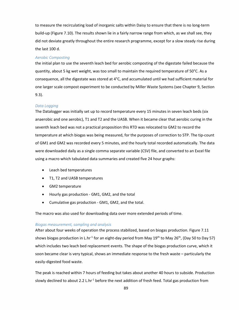
89
to measure the recirculating load of inorganic salts within Daisy to ensure that there is no long-term
build-up (Figure 7.10). The results shown lie in a fairly narrow range from which, as we shall see, they
did not deviate greatly throughout the entire research programme, except for a slow steady rise during
the last 100 d.
Aerobic Composting the initial plan to use the seventh leach bed for aerobic composting of the digestate failed because the
quantity, about 5 kg wet weight, was too small to maintain the required temperature of 50°C. As a
consequence, all the digestate was stored at 4°C, and accumulated until we had sufficient material for
one larger scale compost experiment to be conducted by Miller Waste Systems (see Chapter 9, Section
9.3).
Data Logging The Datalogger was initially set up to record temperature every 15 minutes in seven leach beds (six
anaerobic and one aerobic), T1 and T2 and the UASB. When it became clear that aerobic curing in the
seventh leach bed was not a practical proposition this RTD was relocated to GM2 to record the
temperature at which biogas was being measured, for the purposes of correction to STP. The tip-count
of GM1 and GM2 was recorded every 5 minutes, and the hourly total recorded automatically. The data
were downloaded daily as a single comma separate variable (CSV) file, and converted to an Excel file
using a macro which tabulated data summaries and created five 24 hour graphs:
Leach bed temperatures
T1, T2 and UASB temperatures
GM2 temperature
Hourly gas production - GM1, GM2, and the total
Cumulative gas production - GM1, GM2, and the total.
The macro was also used for downloading data over more extended periods of time.
Biogas measurement, sampling and analysis After about four weeks of operation the process stabilized, based on biogas production. Figure 7.11
shows biogas production in L.hr-1 for an eight-day period from May 19th to May 26th, (Day 50 to Day 57)
which includes two leach bed replacement events. The shape of the biogas production curve, which it
soon became clear is very typical, shows an immediate response to the fresh waste – particularly the
easily-digested food waste.
The peak is reached within 7 hours of feeding but takes about another 40 hours to subside. Production
slowly declined to about 2.2 L.hr-1 before the next addition of fresh feed. Total gas production from
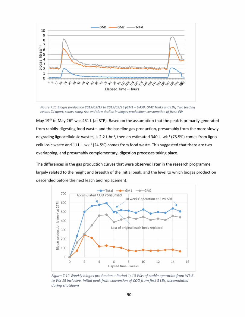
90
May 19th to May 26th was 451 L (at STP). Based on the assumption that the peak is primarily generated
from rapidly-digesting food waste, and the baseline gas production, presumably from the more slowly
degrading lignocellulosic wastes, is 2.2 L.hr-1, then an estimated 340 L..wk-1 (75.5%) comes from ligno-
cellulosic waste and 111 L .wk-1 (24.5%) comes from food waste. This suggested that there are two
overlapping, and presumably complementary, digestion processes taking place.
The differences in the gas production curves that were observed later in the research programme
largely related to the height and breadth of the initial peak, and the level to which biogas production
descended before the next leach bed replacement.
0
100
200
300
400
500
600
700
0 2 4 6 8 10 12 14 16
Biog
as p
rodu
ctio
n l/w
eek
at 2
97K
Total GM1 GM2
10 weeks' operation at 6 wk SRTAccumulated COD consumed
Last of original leach beds replaced
Figure 7.12 Weekly biogas production – Period 1; 10 Wks of stable operation from Wk 6 to Wk 15 inclusive. Initial peak from conversion of COD from first 3 LBs, accumulated during shutdown
Elapsed time - weeks
0123456789
10
Biog
as l
itres
/hr
Elapsed Time - Hours
GM1 GM2 Total
Figure 7.11 Biogas production 2015/05/19 to 2015/05/26 (GM1 – UASB, GM2 Tanks and LBs) Two feeding events 7d apart; shows sharp rise and slow decline in biogas production; consumption of fresh FW
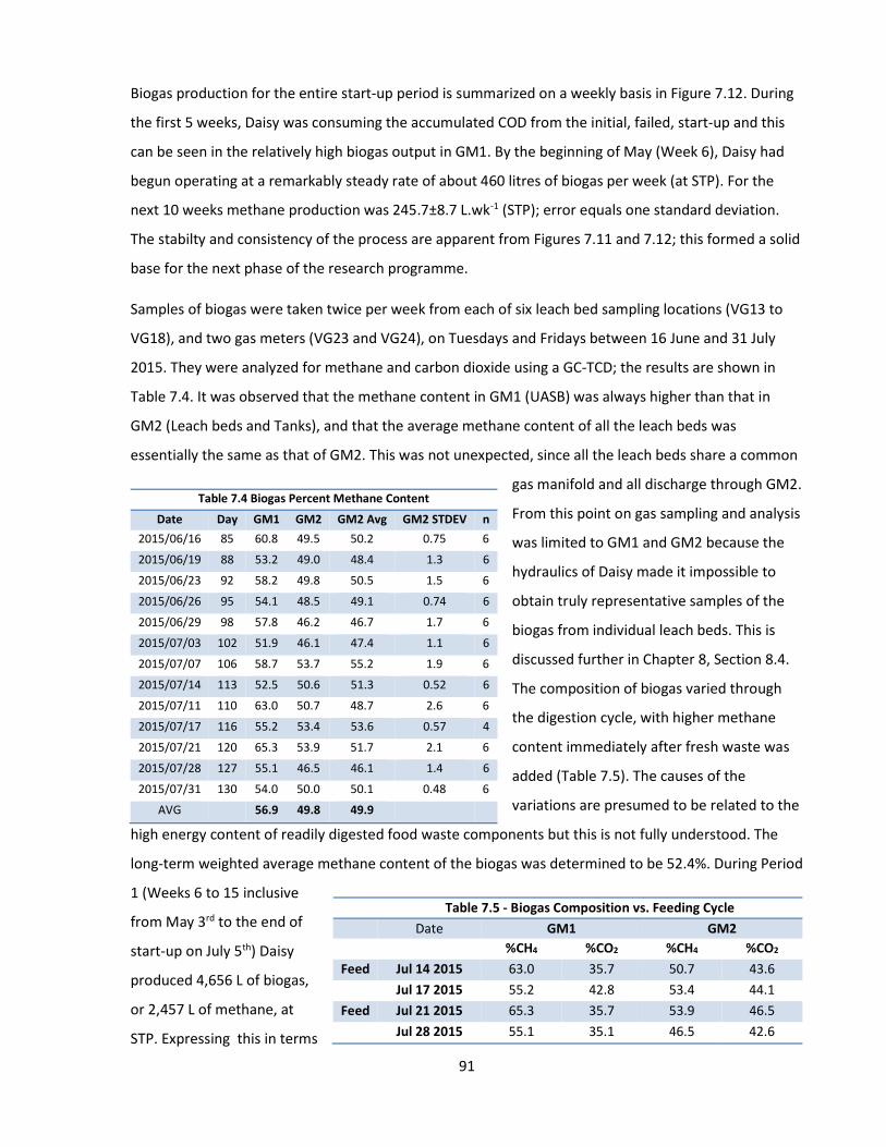
91
Biogas production for the entire start-up period is summarized on a weekly basis in Figure 7.12. During
the first 5 weeks, Daisy was consuming the accumulated COD from the initial, failed, start-up and this
can be seen in the relatively high biogas output in GM1. By the beginning of May (Week 6), Daisy had
begun operating at a remarkably steady rate of about 460 litres of biogas per week (at STP). For the
next 10 weeks methane production was 245.7±8.7 L.wk-1 (STP); error equals one standard deviation.
The stabilty and consistency of the process are apparent from Figures 7.11 and 7.12; this formed a solid
base for the next phase of the research programme.
Samples of biogas were taken twice per week from each of six leach bed sampling locations (VG13 to
VG18), and two gas meters (VG23 and VG24), on Tuesdays and Fridays between 16 June and 31 July
2015. They were analyzed for methane and carbon dioxide using a GC-TCD; the results are shown in
Table 7.4. It was observed that the methane content in GM1 (UASB) was always higher than that in
GM2 (Leach beds and Tanks), and that the average methane content of all the leach beds was
essentially the same as that of GM2. This was not unexpected, since all the leach beds share a common
gas manifold and all discharge through GM2.
From this point on gas sampling and analysis
was limited to GM1 and GM2 because the
hydraulics of Daisy made it impossible to
obtain truly representative samples of the
biogas from individual leach beds. This is
discussed further in Chapter 8, Section 8.4.
The composition of biogas varied through
the digestion cycle, with higher methane
content immediately after fresh waste was
added (Table 7.5). The causes of the
variations are presumed to be related to the
high energy content of readily digested food waste components but this is not fully understood. The
long-term weighted average methane content of the biogas was determined to be 52.4%. During Period
1 (Weeks 6 to 15 inclusive
from May 3rd to the end of
start-up on July 5th) Daisy
produced 4,656 L of biogas,
or 2,457 L of methane, at
STP. Expressing this in terms
Table 7.4 Biogas Percent Methane Content
Date Day GM1 GM2 GM2 Avg GM2 STDEV n 2015/06/16 85 60.8 49.5 50.2 0.75 6
2015/06/19 88 53.2 49.0 48.4 1.3 6
2015/06/23 92 58.2 49.8 50.5 1.5 6
2015/06/26 95 54.1 48.5 49.1 0.74 6
2015/06/29 98 57.8 46.2 46.7 1.7 6
2015/07/03 102 51.9 46.1 47.4 1.1 6
2015/07/07 106 58.7 53.7 55.2 1.9 6
2015/07/14 113 52.5 50.6 51.3 0.52 6
2015/07/11 110 63.0 50.7 48.7 2.6 6
2015/07/17 116 55.2 53.4 53.6 0.57 4
2015/07/21 120 65.3 53.9 51.7 2.1 6
2015/07/28 127 55.1 46.5 46.1 1.4 6
2015/07/31 130 54.0 50.0 50.1 0.48 6
AVG
56.9 49.8 49.9
Table 7.5 - Biogas Composition vs. Feeding Cycle Date GM1 GM2
%CH4 %CO2 %CH4 %CO2
Feed Jul 14 2015 63.0 35.7 50.7 43.6 Jul 17 2015 55.2 42.8 53.4 44.1
Feed Jul 21 2015 65.3 35.7 53.9 46.5 Jul 28 2015 55.1 35.1 46.5 42.6

92
of COD, at 350 mL of methane per 1.0 g COD destroyed, shows that Daisy converted 7,020 g of COD to
methane.
Feedstock destruction efficiency and COD mass balance It was decided from the beginning that the measurement of Daisy’s performance would be based
primarily on COD measurements. The analytical task to do this is more challenging and time-consuming
than the more usual VS measurements, but the calculation of the mass balance is more robust and
useful because it is essentially on the basis of electron equivalents and does not rely upon knowing the
oxidation state of the substrates. Nevertheless, destruction as TS and VS were measured throughout
for the purposes of comparing the results of this study with the published literature which more
commonly uses TS/VS rather than COD measurements. The substrate destruction efficiency was
determined as mass, volatile solids and COD on a weekly basis from the analysis of the digestate. It was
calculated in two ways, with and without bulking agent. The former is the more accurate and simpler to
calculate, but the latter measures substrate destruction, one of the principal objectives of the research,
and is thus important. Because a small amount of the bulking agent is digested, and contributes to
biogas production, the destruction efficiency of the bulking agent alone must be determined in order to
calculate substrate destruction efficiency separately. Data from the coupon technique (Section 6.1e)
was used to make this determination; it showed that, depending upon operating conditions, the
destruction of bulking agent ranged from 2% to 10% and averaged approximately 7%. The two
calculations, with and without bulking agent, are explained in Figure 7.13 using the digestate from
S.012 as an example. The coupons were first used in S.015, so the value for Y came from subsequent
analytical results. Table 7.6 shows the destruction efficiency results for Period 1, calculated both with
Using S.012 as the example:
Method 1 – Including BA
Destruction Efficiency = (CODFW+FB+BA – CODDG)/CODFW+FW+BA*100%
Destruction Efficiency = (2096 – 1180)/2096*100 = 43.7%
Method 2 – Excluding BA
Destruction Efficiency = (CODFW+FB – (CODDG – [CODBA (100 – y)]/100))/CODFW+FB*100%
Destruction Efficiency = (1452 – (1180 – [645(100-7.04)/100]))/1452*100% = 60.0%
Y = BA destruction efficiency = 7.04% in this example
Figure 7.13 Sample calculation of COD destruction efficiency, with and without bulking agent

93
and without bulking agent. These data formed the baseline against which to compare Daisy’s
performance under different operating conditions and feedstock composition.
To assess Daisy’s performance, and the dependability of the analytical data, a mass balance calculation
was performed for Period 1; the results are presented in Table 7.7.
Table 7.6 Substrate Destruction Efficiency – Period 1
Serial No.
Percent Destruction Efficiency
Mass VS COD
With BA Without BA With BA Without BA With BA Without BA
S.008 41.9 55.7 46.1 63.1 43.5 59.7
S.009 37.4 49.5 41.6 56.6 39.2 53.5
S.010 35.5 46.8 39.6 53.8 37.3 50.8
S.011 38.1 50.4 42.0 57.3 39.3 53.6
S.012a 40.5 53.9 46.3 63.4 43.7 60.0
S.013 42.3 56.3 47.1 64.6 44.6 61.3
S.014 36.8 48.7 42.2 57.6 39.5 53.9
S.015b 36.1 47.7 40.7 55.3 37.9 51.5
S.016b 34.9 46.0 39.7 53.9 36.8 50.0
S.017b 30.4 39.7 34.9 47.1 31.8 42.9
Average 37.4 49.5 42.0 57.3 39.4 53.7 aSee calculation in Figure 5.3.14 b the FW in these Leach beds was not blended
Table 7.7 COD Mass Balance at Start-up – Period 1
Week Serial No.
COD g Methane
(a)
Substr. in
(b) DG out
(c) Destr. (d) conv. cells
(e) Conv. CH4 (f) Vol. out L (g) as COD out g.
Mass Bal. %
wkly cum. wkly cum. wkly cum. wkly cum. wkly cum.
6 S.008 2100 1180 913 910 73.0 73.0 840 840 246 246 702 702 83.5
7 S.009 2100 1280 822 1740 65.8 139 756 1600 253 498 721 1420 95.4
8 S.010 2100 1310 783 2520 62.6 201 720 2320 248 746 708 2130 98.3
9 S.011 2100 1270 824 3340 65.9 267 758 3070 237 983 677 2810 89.3
10 S.012 2100 1180 917 4260 73.4 341 844 3920 254 1240 726 3530 86.1
11 S.013 2100 1160 936 5190 74.8 416 861 4780 232 1470 664 4200 77.2
12 S.014 2100 1270 828 6020 66.3 482 762 5540 243 1710 695 4890 91.1
13 S.015p 2100 1300 794 6820 63.5 545 731 6270 238 1950 680 5570 93.1
14 S.016p 2100 1330 772 7590 61.8 607 710 6980 261 2210 747 6320 105.1
15 S.017p 2100 1430 668 8260 53.5 661 615 7600 245 2460 700 7020 113.9
Totals 20970 12710 8260 660 7596 2460 7020 92.4
c = a - b d = c*0.08 e = c - d g = f/0.35l.gCOD-1 Mass bal. = 7020/7596*100% = 92.4 %
mass balance = g/e*100% = 92.4% p the FW in these leach beds was not blended
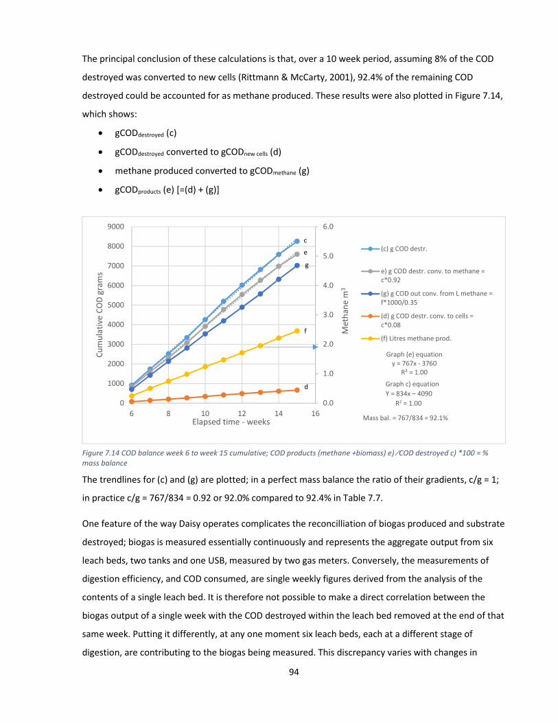
94
The principal conclusion of these calculations is that, over a 10 week period, assuming 8% of the COD
destroyed was converted to new cells (Rittmann & McCarty, 2001), 92.4% of the remaining COD
destroyed could be accounted for as methane produced. These results were also plotted in Figure 7.14,
which shows:
gCODdestroyed (c)
gCODdestroyed converted to gCODnew cells (d)
methane produced converted to gCODmethane (g)
gCODproducts (e) [=(d) + (g)]
The trendlines for (c) and (g) are plotted; in a perfect mass balance the ratio of their gradients, c/g = 1;
in practice c/g = 767/834 = 0.92 or 92.0% compared to 92.4% in Table 7.7.
One feature of the way Daisy operates complicates the reconcilliation of biogas produced and substrate
destroyed; biogas is measured essentially continuously and represents the aggregate output from six
leach beds, two tanks and one USB, measured by two gas meters. Conversely, the measurements of
digestion efficiency, and COD consumed, are single weekly figures derived from the analysis of the
contents of a single leach bed. It is therefore not possible to make a direct correlation between the
biogas output of a single week with the COD destroyed within the leach bed removed at the end of that
same week. Putting it differently, at any one moment six leach beds, each at a different stage of
digestion, are contributing to the biogas being measured. This discrepancy varies with changes in
Graph (e) equationy = 767x - 3760
R² = 1.00
0.0
1.0
2.0
3.0
4.0
5.0
6.0
0
1000
2000
3000
4000
5000
6000
7000
8000
9000
6 8 10 12 14 16
Met
hane
m3
Cum
ulat
ive
COD
gram
s
Elapsed time - weeks
(c) g COD destr.
e) g COD destr. conv. to methane =c*0.92
(g) g COD out conv. from L methane =f*1000/0.35
(d) g COD destr. conv. to cells =c*0.08
(f) Litres methane prod.
c
d
e
f
g
Mass bal. = 767/834 = 92.1%
Figure 7.14 COD balance week 6 to week 15 cumulative; COD products (methane +biomass) e) ∕COD destroyed c) *100 = % mass balance
Graph c) equation Y = 834x – 4090 R2 = 1.00

95
operating conditions, including FW addition. This only really matters when looking for short term
relationships; under steady operating conditions it is not material.
Wastewater Daisy produces no free wastewater. The only water leaving the digester is the water within the
digestate; approximately 3.8L per week, and as water vapour in the biogas amounting to about 2.5% by
volume (140 g over the 15 week start-up period). When liquid samples are withdrawn they are replaced
in like quantity with de-ionized water. Daily records of leachate withdrawal and replacement were
maintained throughout. Tests were conducted on the feedstock and the digestate to determine if the
lack of free waste water was causing an increase in the recirculating load of inorganic material in
solution or suspension (Figure 7.10). The initial concentration, when Daisy was restarted, was greater
than 5.0 g.L-1. It rapidly dropped to 3.49 g.L-1, and for the next 60 days remained between 2.99 and 3.64
g.L-1. The total inorganic content of the feedstock in each leach bed was determined to be 160 g, and
the same determination on four samples of digestate averaged 171 g, thus the inorganic components
of the feedstock/digestate, in and out, were in balance.
Other observations and operating challenges Figure 7.15 shows Daisy’s Daily Log for June 8 2015, and Figure 7.16 shows the data logger output for
the same day, converted using the macro and reached through the data file hyperlink. This particular
date was chosen because it shows the effects on performance of a leach bed of fresh waste inserted at
16.10 h. Figure 7.16 a) shows the leach bed temperatures; the fresh leach bed (LL02, S.014) can be seen
rising to meet the others, all of which can be seen to be rising slightly. Figure 6.16 b) shows the tank
temperatures rising also. The slightly spiked lines in these two graphs track the valve sequencer cycle
and represent real temperature fluctuations. Biogas production begins to rise within an hour of
installation of the fresh leach bed - Figure 6.16 c) - peaks about five hours later, then begins its slow
decline. During this phase the percentage of biogas produced in the UASB climbs sharply, reflecting the
surge in soluble COD associated with the fresh food waste. Lastly, Figure 6.16 d) shows cumulative gas
production, and linear trend lines with poor regression coefficients. On the other six days of the week
the regression coefficients are generally 0.97 or better; the hourly average biogas generation rates
from GM1 and GM2, and the total, were always recorded in the Daily Log.
Daisy is simple to run; three pumps and six automatic three-way valves are the only moving parts and
all worked flawlessly through commissioning and startup. When it became apparent that a pump
failure could be a serious setback to the research programme, a spare pump was purchased as a back-
up. Other idiosyncrasies were discovered, largely relating to hydraulic behaviour. For example, because
the system is always under slight pressure (12 cm of water – the head in the gas meters), a new leach
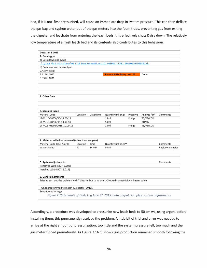
96
bed, if it is not first pressurized, will cause an immediate drop in system pressure. This can then deflate
the gas bag and syphon water out of the gas meters into the foam traps, preventing gas from exiting
the digester and leachate from entering the leach beds; this effectively shuts Daisy down. The relatively
low temperature of a fresh leach bed and its contents also contributes to this behaviour.
Accordingly, a procedure was developed to pressurize new leach beds to 50 cm wc, using argon, before
installing them; this permanently resolved the problem. A little bit of trial and error was needed to
arrive at the right amount of pressurization; too little and the system pressure fell, too much and the
gas meter tipped prematurely. As Figure 7.16 c) shows, gas production remained smooth following the
Date: Jun 8 2015 1. Datalogger a) Data download Y/N:Y ..\..\Data File 1 - Data Taker\06 2015 Excel Format\Jun 8 2015 099017_JOB1_20150609T065811.xls b) Comments on data output 2.43 l/h Total 2.11 l/h GM2 Re-seat RTD fitting on LL02 Done 0.33 l/h GM1 2. Other Data 3. Samples taken Material Code Location Date/Time Quantity (ml or g) Preserve Analyze for* Comments LT-VU15-08/06/15-14.00-15 15ml Fridge TS/VS/COD LT-VU15-08/06/15-14.00-50 50ml pH/alk LT-VL05-08/06/2015-10.00-15 15ml Fridge TS/VS/COD 4. Material added or removed (other than samples) Material Code (plus A or R) Location Time Quantity (ml or g)** Comments Water added T2 14.05h 80ml Replaces samples
5. System adjustments Comments Removed LL02 (LB07, S.008) Installed LL02 (LB07, S.014) 6. General Comments Tried to sort out the problem with T1 heater but to no avail. Checked connectivity in heater cable - OK reprogrammed to match T2 exactly - OK(?). Sent note to Omega
Figure 7.15 Example of Daily Log June 8th 2015; data output; samples; system adjustments

97
installation of the fresh leach bed; the problem had been solved by June 8, 2015.
25
35
45
0 1 2 3 4 5 6 7 8 9 10 11 12 13 14 15 16 17 18 19 20 21 22 23
Tem
pera
ture
Deg
. C
Elapsed Time Hrs
a) Leach Bed Temperatures2015-06-08
LB1 (degC) LB2 (degC) LB3 (degC)
LB4 (degC) LB5 (degC) LB6 (degC)
25
30
35
40
45
0 1 2 3 4 5 6 7 8 9 10 11 12 13 14 15 16 17 18 19 20 21 22 23
Tem
pera
ture
Deg
. C
Elapsed Time Hrs
b) Tank 1, Tank 2 and UASB Temperatures2015-06-08
Tank1 (degC) Tank2 (degC) UASB Bottom (degC)
0
2
4
6
8
1 2 3 4 5 6 7 8 9 10 11 12 13 14 15 16 17 18 19 20 21 22 23 24
Biog
as l
itres
/hr
Elapsed Time Hrs
c) Biogas Production2015-06-08
GM1 GM2 Total
y = 0.33x - 1.09R² = 0.80
y = 2.11x - 4.54R² = 0.94
y = 2.44x - 5.64R² = 0.92
-20
0
20
40
60
80
1 2 3 4 5 6 7 8 9 10 11 12 13 14 15 16 17 18 19 20 21 22 23 24
Biog
as P
rodu
ced
litre
s
Elapsed Time Hrs
d) Cumulative Biogas Production2015-06-08
GM1 GM2 Total
Figure 7.16 Datalogger output, June 8, 2015; a) LB temps; b)Tanks and UASB temps; c) biogas hourly; d) biogas cumulative GM1, GM2 and Total. Fresh leach bed installed at 14:30h. All raw data can be found in EDF1

98
EDF2 contains a complete set of Daily Logs and EDF1 contains all the raw data from the datalogger.
The hydraulic behaviour also makes it very difficult to measure biogas production from the leach beds,
either individually or collectively. To make this measurement it is necessary to separate the leach-bed
headspace from the tank headspace. When this was tried it resulted in rapid process upset in the form
of water syphoning, and had to be quickly reversed. Because the leachate is pumped to the leach beds
from Tank 2 and returns from the leach beds to Tank 1, the leachate withdrawn from T2 causes the
transfer of an equal volume of gas from the leach-bed headspace to the tank headspace to
compensate. The dynamics of this arrangement move larger volumes of biogas back and forth, in a
period of a few minutes, than the system generates during the same period, making biogas
measurement extremely difficult.
Much later in the research programme I did have limited success measuring gas production from
individual leach beds, but this could only be accomplished by cutting off leachate feed for the duration
of the test, which was generally about four hours, and isolating the leach bed entirely except for the gas
line to GM1 to prevent transfer of biogas through the waste mass. This is described more fully in
Chapter 8, Section 8.4. The control system, with the exception of the heater problem, worked perfectly,
as did the gas meters. On July 5th 2015 (day 104) after 70 days of very stable operation the startup
phase, Period 1, was determined to be complete.
7.5 Commissioning and Start-up Conclusions
The commissioning and start-up process accomplished many things and these are summarized below;
but two overarching conclusions can now be reached; firstly, this configuration of digester is capable of
reliably digesting a mixed organic waste stream for an extended period of time (15 weeks) without
process upset; Daisy worked. Secondly, the experience and data gained during the commissioning
period established a series of operational sampling and analytical procedures, and a performance
baseline against which to compare future results.
Summary Period 1, operation with solid waste in the final phase of startup, ran for 104 days. It began with 10 specific objectives; all of which were met. Biogas production at 509.5±3.5% L.wk-1 (297K) and methane production at 245.7±3.5% L.wk-1
(STP) was very stable. Methane production was unaffected when FW blending was eliminated. The following questions were answered:
o pressure loss in the system following leach bed installation was solved by pressurization o a leak testing procedure for leach beds was established

99
o a technique for measuring leach bed permeability in situ was devised o a technique for measuring substrate digestibility was developed o a recurring heater problem was finally solved.
The following problems were deferred: o small-scale aerobic curing did not work; a separate subsequent experiment with
accumulated digestate was devised. o attempts to measure biogas from the leach beds alone caused serious hydraulic
imbalance and failed; data gathered in subsequent experiments suggest that gas production occurs in all leach beds after fresh waste added.
o Daisy was found to have one operational drawback; the lack of ability to test substrate destruction efficiency versus SRT. This was eventually solved, but only in a single experiment at the very end (Week 88), when Daisy was shut down and all six leach beds, at different stages of digestion, were removed at the same time.
The following data management practices were established: o a step-by-step procedure for removing and replacing leach beds. o a complete record of the setup and contents of each leach bed. o a daily electronic log of all operating activities with a hyperlink to the daily download
from the data logger. o a continuous weekly record of biogas production. o electronic data files for all analyzes performed.
The following variables were set: o Vup o temperatures o SRT o settings for the data logger
The following knowledge was gained: o the profile of hourly gas production was established. o COD concentration correlates with the feeding cycle. o the use of the alkalinity ratio is a valuable indicator of digester stability. o the correlation between substrate destruction and biogas production was clearly
demonstrated. o a method to calculate substrate destruction efficiency, both with and without bulking
agent, was established. o Daisy produces no free wastewater o further refinement of the procedures used for feeding, digestate removal, sampling,
and analysis is possible.
Commissioning and startup went as smoothly as one could have hoped and Daisy performed as well as,
or better than, anticipated; the groundwork was laid for the main part of the research programme –
testing the hypothesis.

100
Chapter 8. Operation of Daisy - Results
8.1 Introduction
The experimental programme was planned to test the hypothesis by measuring the effects of changes
in feedstock composition and operating variables on the performance and stability of Daisy.
The initial plan was to test five variables in the following order:
a) solids retention time
b) quantity of food waste in the substrate (expressed as %CODFW)
c) leachate recirculation through the leach beds - volume and frequency
d) bulking agent addition rate
e) UASB functionality; how does it perform and is it needed
The measurement tools to be used were biogas production and composition, substrate destruction,
leachate properties – specifically pH and alkalinity, COD content and VFA concentration, and C:N ratio.
For reasons that will become clear, the programme ultimately concentrated on variables a), b), and a
variant of d).
Daisy was operated for 88 consecutive weeks, divided into six operating periods (including Period 1 –
Startup described in Chapter 7); data from Weeks 1 to 5 inclusive were omitted from long-term
calculations because of irregularities in the feeding and operating plan related to start-up. Table 8.1
summarizes the dates and durations (in weeks and days) of the six operating Periods; it also includes
the Serial numbers of the leach beds in place at the time, and a brief description of the objective for
each Period. Table 8.2 describes operating conditions prevailing in each operating Period. The principal
changes were the amount of food waste added to the fibres during Periods 4, 5 and 6, and changes in
bulking agent during Period 5.
All of the assessments of Daisy’s performance, and the major conclusions drawn, rest on three separate
sets of data:
COD measurements of substrate and digestate; these were carried out in sextuplicates rather than the usual triplicates because of the heterogeneity of the substrates.
Biogas volumes; these were converted to methane at STP using gas analysis data and temperature and pressure measurements. The average of 40 separate measurements of biogas composition was used.

101
Elemental analyzes of all substrates (duplicate tests of three separate sets of samples) were used to verify the COD methodology and results, calculate the stoichiometry of the process and predict the methane content of the biogas.
Together, these form the basis of the discussion presented in Section 8.3. The culmination of all of
these sets of data is the 83 week, COD-based, mass balance of Daisy, which shows that 100.8% of the
COD destroyed can be accounted for as methane produced plus new cell growth. The latter was
calculated as 8% of COD destroyed based on Rittmann & McCarty (2001). To the best of my ability to
determine from the literature, an AD experiment of this duration has never been accompanied by a
COD-based mass balance. Given the duration of the experiment, and the diversity of the measurements
used to obtain this result, I would argue that the mass balance lends credibility to the results and
conclusions of this thesis. The bulk of the performance data, except BMPs, synergy, permeability and
enzyme activity are summarized in EDF4.
Table 8.1 Experimental Periods
Period Dates (inclusive) Weeks Days Sub
periods LB Serial No. Description Comments
1 Mar 24 - Jul 5 2015 1 to 15 1 to 104 2 S.001 to S.017 Commissioning Data from
weeks 1 to 5 excluded
2 Jul 5 to Sep 6 2015 16 to 24 105 to 167 none S.018 to S.024 7 wk. SRT
3 Sep 7 to Oct 26 2015
25 to 31 168 to 217 none S.025 to S.031 Return to 6wk. SRT
4 Oct 27 2015 to Feb 29 2016
32 to 49 218 to 343 3 S.032 to S.048 CODFW 17% to 0% in 3 steps
Synergy observed
5 Mar 1 to Aug 22
2016 50 to 74 344 to 518 4 S.049 to S.073 Return to
CODFW 17% in 1 step.
Bulking agent effect
6 Aug 23 to Nov 28
2016 85 to 88 519 to 616 2 S.074 to S.087
CODFW to 55% in 2 steps
The results are presented and discussed from three different perspectives in three different
subsections, each one of which of tells a different part of the story.
Firstly the long view, looking at the experiment in its entirety, presents an assessment of
process robustness and stability under changing conditions, both deliberate and accidental,
using several different sets of data.
Secondly, a closer examination of performance Period by Period provides an analysis of
lengthening the SRT to 7 weeks, the synergistic effect of food waste addition on the digestion

102
of fibres, and an analysis of unexpected changes in performance apparently related to the
properties of the bulking agent.
Thirdly, an examination of short-term trends – hourly and daily – explains how Daisy responded
to short-term changes in operating conditions and defines some of the benefits of the
sequentially batch-fed design concept.
Throughout the research programme five supporting experiments were conducted to gain a deeper
understanding of Daisy’s performance and the mechanisms behind the observed behaviour; these
were:
leach bed permeability tests
leach bed biogas production tests
biochemical methane potential tests (BMPs)
enzyme assays
aerobic curing of digestate
Table 8.2 Daisy's Operating Conditions
Period CODFW %
total COD
UASB Vup m.h-1
Pump Settings rpm/ml.min-1
Temperature settings °C
Bulking Agent Batch
1 2 3 T1 T2 UASB
1 17.2 0.1/0.15 125/120 55/100 167/510 37 39 37 1 & 2
2 17.2 0.15 125/120 55/100 167/510 37 39 37 2 & 3
3 17.2 0.15 125/120 55/100 167/510 37 39 37 3
4a 12.9 0.15 125/120 55/100 167/510 37 39 37 4
4b 7.9 0.15 125/120 55/100 167/510 37 39 37 4
4c 0 0.15 125/120 55/100 167/510 37 39 37 4
5a 17.2 0.15 125/120 55/100 167/510 37 39 37 4
5b 17.2 0.15 125/120 55/100 167/510 37 39 37 5
5c 17.2 0.15 125/120 55/100 167/510 37 39 37 4
5d 17.2 0.15 125/120 55/100 167/510 37 39 37 6
6a 21.7 0.15 125/120 55/100 167/510 37 39 37 7
6b 29.3 0.15 125/120 55/100 167/510 37 39 37 8
The first two supporting experiments are incorporated in this chapter, in Section 8.3. The last three are
described in Chapter 9. The discussion of results, presented in Chapter 10, interprets the operating data
with the help of the supporting experiments. The graphs and tables are all colour-coded by period for
ease of reference.

103
8.2 Overall Performance – Robustness and Stability
Long-term performance was tracked with seven different measurements, substrate destruction (as
mass, VS and COD), biogas production, pH and alkalinity and concentrations of total inorganic salts,
sulphate, COD, and VFAs within Daisy. The data are first described, then discussed in the context of
stability and robustness.
8.2.1 Substrate Destruction and Biogas Production
In Figure 8.1, substrate destruction is expressed on the basis of TS, VS, and COD. The VS and COD
measurements correspond quite closely; TS destruction efficiency is lower because the inorganic
matter present in the waste is also present in the digestate. COD destruction efficiency is used
throughout for calculating the mass balance. The VS destruction efficiency is used primarily to make
comparisons with work published by others.
Figure 8.2 presents weekly biogas production expressed as L.wk-1 at 297K. By comparing Figures 8.1 and
8.2 it is clear that destruction efficiency and biogas production follow similar paths. The
correspondence is not exact because there are always six leach beds contributing to the biogas
measured in any one week, making it hard to achieve exact correlation between substrate destruction
and biogas production. This can be illustrated by two apparent anomalies; the sharp drop in gas
production around Week 25 (Figure 8.2) occurred during a 10-day period during which the heaters and
0
10
20
30
40
50
60
70
80
0 10 20 30 40 50 60 70 80 90
Dest
ruct
ion
Rate
[%]
Leach Bed Serial Number (over 88 weeks)
TS Destruction VS Destruction COD Destruction
P1 P2 P3 P4 P5 P6
Figure 8.1 Substrate destruction efficiency as TS, VS and COD vs. time (calculated without BA). Destruction efficiency ranges from 18 to 70% on a COD basis and rises and falls with CODFW addition

104
valve sequencer were turned off and Daisy was not fed, but there was no corresponding decline in
substrate destruction during that same period (Figure 8.1). When Daisy was turned back on, the biogas
production rate rose beyond where it had been previously, but there was no corresponding rise in
substrate destruction; the six week average biogas production through this period was 483 L.wk-1, only
5% lower than in Period 1.
Table 8.3 COD Substrate Destruction Efficiency by Period
Operating Data Mass VS COD
Period Weeks Serial Nos. With BA Without BA With BA Without BA With BA Without BA
1 6 - 15 S.008 - S.017 37.4 49.5 42.0 57.3 39.4 53.7
2 16 - 24 S.018 - S.024 37.1 49.0 42.7 58.2 39.2 53.5
3 25 - 31 S.025 - S.030 37.2 49.2 43.4 59.3 39.7 54.2
4a 32 - 37 S.030 - S.035 27.8 36.0 32.2 43.2 29.1 38.9
4b 38 - 44 S.036 - S.042 21.1 28.7 23.7 33.2 22.6 31.8
4c 44 - 49 S.043 - S.048 13.4 17.5 14.8 20.0 13.7 18.6
5a 50 - 57 S.049 - S.056 36.4 48.0 39.1 53.1 37.9 51.7
5b 58 - 63 S.057 - S.062 32.0 41.9 34.1 45.9 32.5 43.8
5c 64 - 70 S.063 - S.068 32.7 43.0 36.1 48.7 32.5 43.9
5d 71 - 74 S.069 - S.073 36.8 48.6 41.3 56.3 38.9 53.0
6a 74 - 80 S.074 - S.079 41.1 54.2 46.8 63.5 41.3 56.0
6b 81 - 88 S.080 - S.087 48.3 61.8 52.9 69.4 49.9 65.3
Totals 6 - 88 S.008 - S.087 33.7 44.3 37.7 51.0 34.9 47.2
Table 8.3 is a summary, by Period, of substrate destruction efficiency expressed as mass, VS and COD,
both with and without bulking agent. The average destruction efficiencies (corresponding to periods of
stable biogas production at each level of CODFW addition) range from 18.6% to 65% (calculated without
0
100
200
300
400
500
600
700
800
900
0 10 20 30 40 50 60 70 80 90
Biog
as P
rodu
ctio
n L/
wk.
at 2
97K
Elapsed Time - weeks
513L/wk.
797L/wk.
620L/wk.Stable Biogas Production
509L/wk 414L/wk.
287L/wk.
132L/wk.
Figure 8.2 Weekly biogas production showing periods of stable biogas production at different levels of CODFW addition.
509L/wk
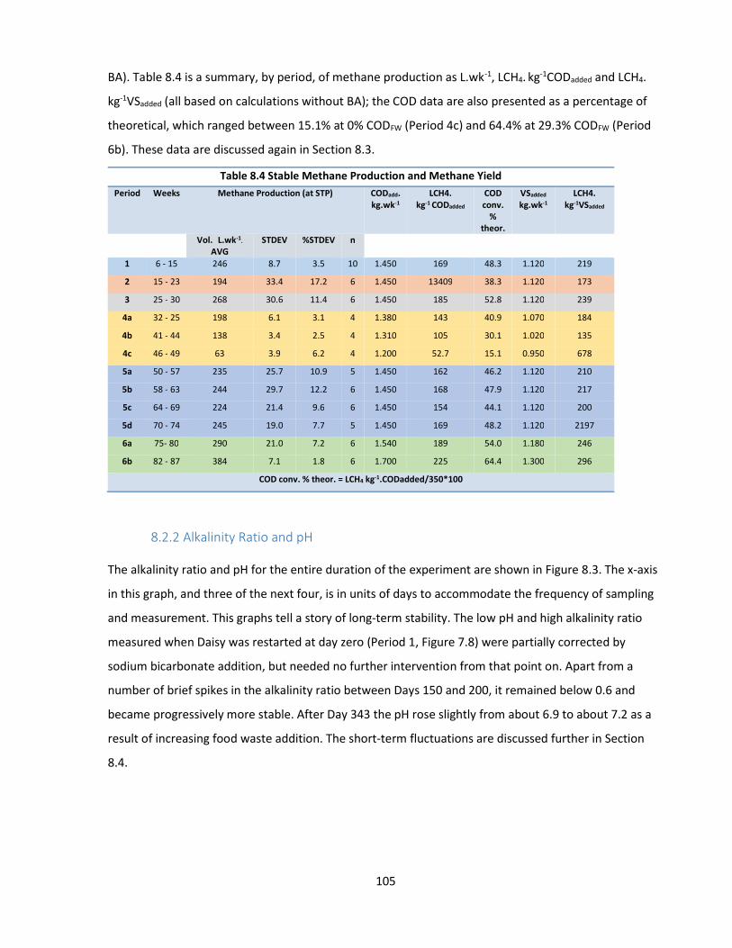
105
BA). Table 8.4 is a summary, by period, of methane production as L.wk-1, LCH4. kg-1CODadded and LCH4.
kg-1VSadded (all based on calculations without BA); the COD data are also presented as a percentage of
theoretical, which ranged between 15.1% at 0% CODFW (Period 4c) and 64.4% at 29.3% CODFW (Period
6b). These data are discussed again in Section 8.3.
8.2.2 Alkalinity Ratio and pH
The alkalinity ratio and pH for the entire duration of the experiment are shown in Figure 8.3. The x-axis
in this graph, and three of the next four, is in units of days to accommodate the frequency of sampling
and measurement. This graphs tell a story of long-term stability. The low pH and high alkalinity ratio
measured when Daisy was restarted at day zero (Period 1, Figure 7.8) were partially corrected by
sodium bicarbonate addition, but needed no further intervention from that point on. Apart from a
number of brief spikes in the alkalinity ratio between Days 150 and 200, it remained below 0.6 and
became progressively more stable. After Day 343 the pH rose slightly from about 6.9 to about 7.2 as a
result of increasing food waste addition. The short-term fluctuations are discussed further in Section
8.4.
Table 8.4 Stable Methane Production and Methane Yield Period Weeks Methane Production (at STP) CODadd.
kg.wk-1 LCH4.
kg-1 CODadded COD conv.
% theor.
VSadded kg.wk-1
LCH4. kg-1VSadded
Vol. L.wk-1.
AVG STDEV %STDEV n
1 6 - 15 246 8.7 3.5 10 1.450 169 48.3 1.120 219
2 15 - 23 194 33.4 17.2 6 1.450 13409 38.3 1.120 173
3 25 - 30 268 30.6 11.4 6 1.450 185 52.8 1.120 239
4a 32 - 25 198 6.1 3.1 4 1.380 143 40.9 1.070 184
4b 41 - 44 138 3.4 2.5 4 1.310 105 30.1 1.020 135
4c 46 - 49 63 3.9 6.2 4 1.200 52.7 15.1 0.950 678
5a 50 - 57 235 25.7 10.9 5 1.450 162 46.2 1.120 210
5b 58 - 63 244 29.7 12.2 6 1.450 168 47.9 1.120 217
5c 64 - 69 224 21.4 9.6 6 1.450 154 44.1 1.120 200
5d 70 - 74 245 19.0 7.7 5 1.450 169 48.2 1.120 2197
6a 75- 80 290 21.0 7.2 6 1.540 189 54.0 1.180 246
6b 82 - 87 384 7.1 1.8 6 1.700 225 64.4 1.300 296
COD conv. % theor. = LCH4 kg-1.CODadded/350*100

106
8.2.3 Wastewater and Inorganic Salts (including sulphate)
Throughout Period 1, leachate levels within Daisy remained stable, and there was no requirement to
drain wastewater. This behaviour continued through Periods 2 and 3, and it became clear that the
water added to the waste before feeding, water removed with the digestate as water of saturation, and
water consumed, were in near perfect balance. This raised the question of the inorganic salts
circulating within Daisy, and whether their concentration might rise to inhibitory levels. Figure 8.4 was
plotted using data from the ash measurements from the VS analyzes.
1.0
1.5
2.0
2.5
3.0
3.5
4.0
4.5
5.0
0 100 200 300 400 500 600
Conc
entr
atio
n of
inor
gani
c sa
lts g
/L
Elapsed Time - days
P1 P2 P3 P4 P5 P6
Figure 8.4 Concentration of inorganic salts in Daisy – following changes in CODFW addition
5.5
6.0
6.5
7.0
7.5
8.0
0.0
0.20.40.60.8
1.01.21.41.6
1.82.0
0 100 200 300 400 500 600
pH
Alka
linity
Rat
io (I
A/PA
)
Elapsed Time - days
Alkalinity Ratio (IA/PA) pH
P4 P5 P6P1 P2 P3
Figure 8.3 Alkalinity ratio and pH vs. elapsed time; stability under changing levels of FW addition
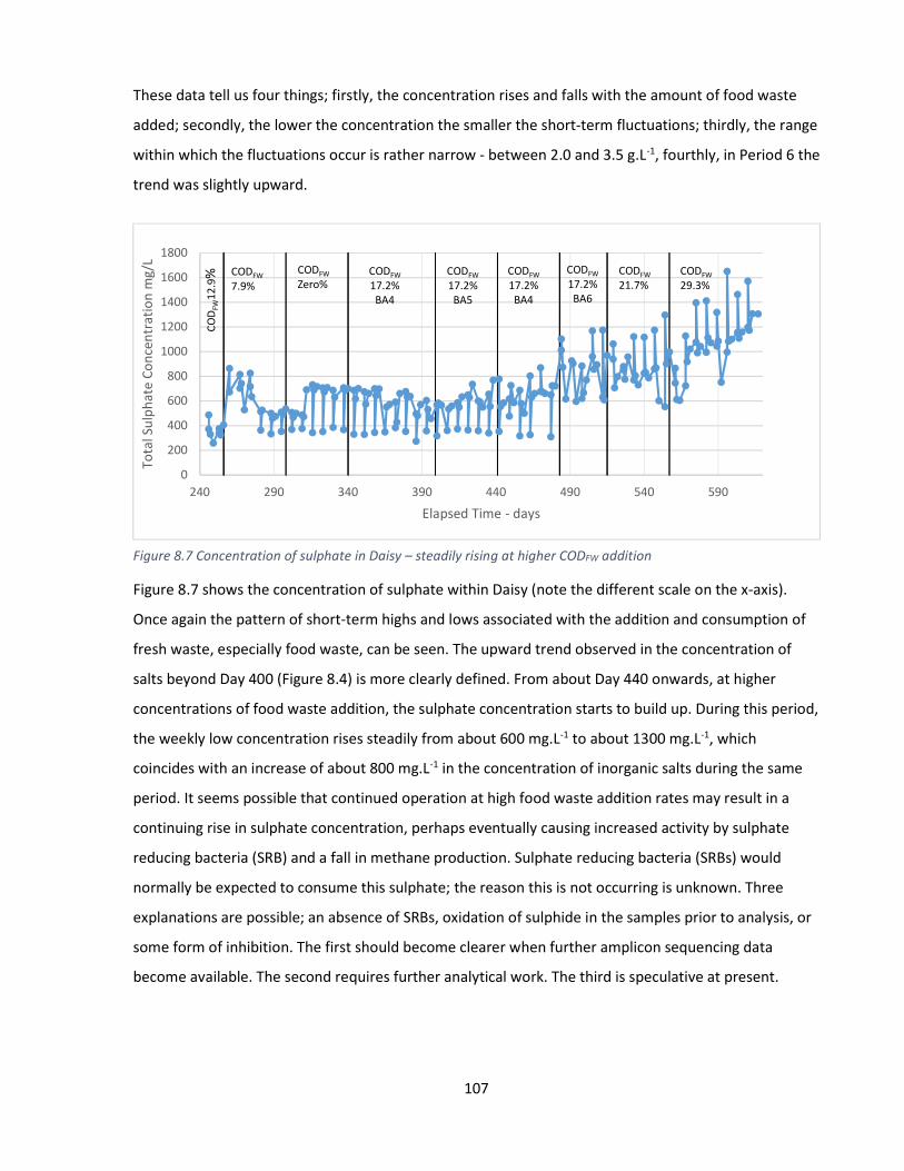
107
These data tell us four things; firstly, the concentration rises and falls with the amount of food waste
added; secondly, the lower the concentration the smaller the short-term fluctuations; thirdly, the range
within which the fluctuations occur is rather narrow - between 2.0 and 3.5 g.L-1, fourthly, in Period 6 the
trend was slightly upward.
Figure 8.7 shows the concentration of sulphate within Daisy (note the different scale on the x-axis).
Once again the pattern of short-term highs and lows associated with the addition and consumption of
fresh waste, especially food waste, can be seen. The upward trend observed in the concentration of
salts beyond Day 400 (Figure 8.4) is more clearly defined. From about Day 440 onwards, at higher
concentrations of food waste addition, the sulphate concentration starts to build up. During this period,
the weekly low concentration rises steadily from about 600 mg.L-1 to about 1300 mg.L-1, which
coincides with an increase of about 800 mg.L-1 in the concentration of inorganic salts during the same
period. It seems possible that continued operation at high food waste addition rates may result in a
continuing rise in sulphate concentration, perhaps eventually causing increased activity by sulphate
reducing bacteria (SRB) and a fall in methane production. Sulphate reducing bacteria (SRBs) would
normally be expected to consume this sulphate; the reason this is not occurring is unknown. Three
explanations are possible; an absence of SRBs, oxidation of sulphide in the samples prior to analysis, or
some form of inhibition. The first should become clearer when further amplicon sequencing data
become available. The second requires further analytical work. The third is speculative at present.
0
200
400
600
800
1000
1200
1400
1600
1800
240 290 340 390 440 490 540 590
Tota
l Sul
phat
e Co
ncen
trat
ion
mg/
L
Elapsed Time - days
CODFW 7.9%
COD
FW12
.9% CODFW
Zero%CODFW 17.2%BA5
CODFW 17.2%BA4
CODFW 17.2%BA6
CODFW 17.2%BA4
CODFW 29.3%
CODFW 21.7%
Figure 8.7 Concentration of sulphate in Daisy – steadily rising at higher CODFW addition
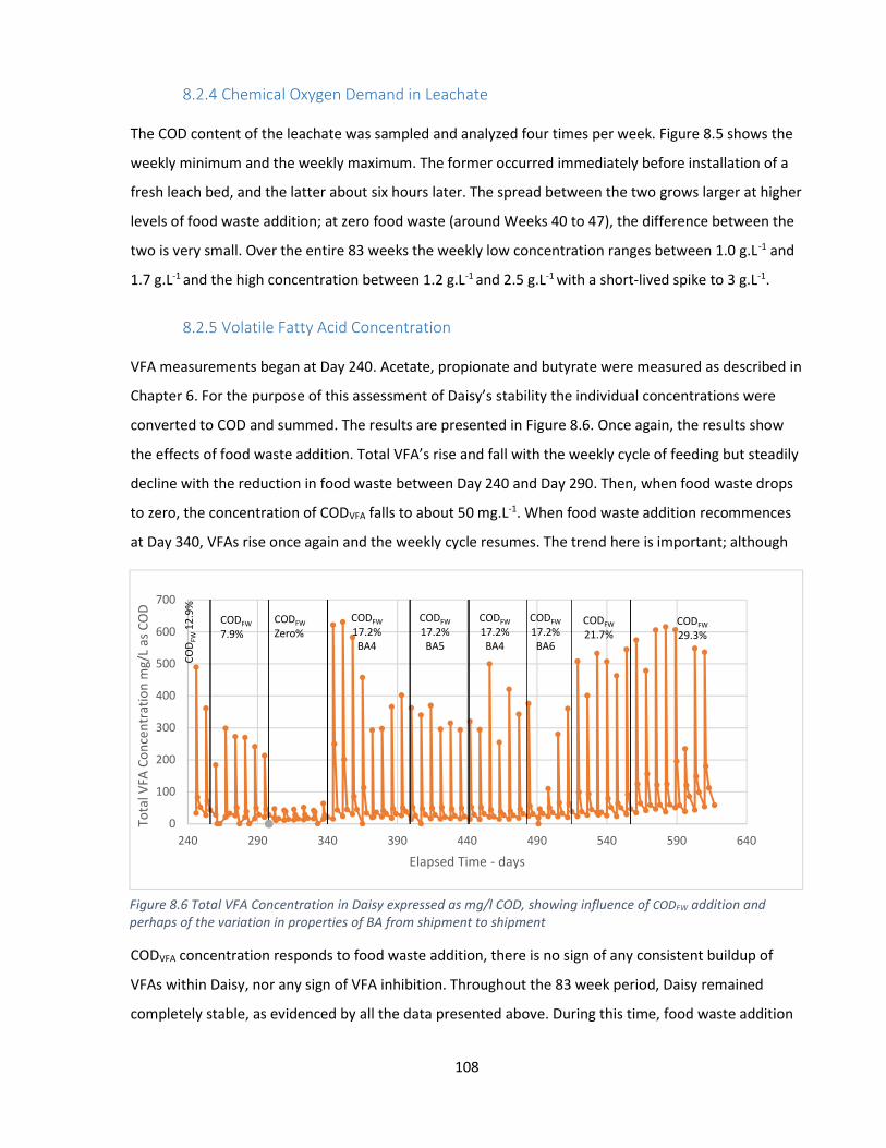
108
8.2.4 Chemical Oxygen Demand in Leachate
The COD content of the leachate was sampled and analyzed four times per week. Figure 8.5 shows the
weekly minimum and the weekly maximum. The former occurred immediately before installation of a
fresh leach bed, and the latter about six hours later. The spread between the two grows larger at higher
levels of food waste addition; at zero food waste (around Weeks 40 to 47), the difference between the
two is very small. Over the entire 83 weeks the weekly low concentration ranges between 1.0 g.L-1 and
1.7 g.L-1 and the high concentration between 1.2 g.L-1 and 2.5 g.L-1 with a short-lived spike to 3 g.L-1.
8.2.5 Volatile Fatty Acid Concentration
VFA measurements began at Day 240. Acetate, propionate and butyrate were measured as described in
Chapter 6. For the purpose of this assessment of Daisy’s stability the individual concentrations were
converted to COD and summed. The results are presented in Figure 8.6. Once again, the results show
the effects of food waste addition. Total VFA’s rise and fall with the weekly cycle of feeding but steadily
decline with the reduction in food waste between Day 240 and Day 290. Then, when food waste drops
to zero, the concentration of CODVFA falls to about 50 mg.L-1. When food waste addition recommences
at Day 340, VFAs rise once again and the weekly cycle resumes. The trend here is important; although
CODVFA concentration responds to food waste addition, there is no sign of any consistent buildup of
VFAs within Daisy, nor any sign of VFA inhibition. Throughout the 83 week period, Daisy remained
completely stable, as evidenced by all the data presented above. During this time, food waste addition
0
100
200
300
400
500
600
700
240 290 340 390 440 490 540 590 640
Tota
l VFA
Con
cent
ratio
n m
g/L
as C
OD
Elapsed Time - days
CODFW 7.9%
COD
FW 1
2.9%
CODFW Zero%
CODFW 17.2%BA5
CODFW 17.2%BA4
CODFW17.2%BA6
CODFW 17.2%BA4
CODFW 29.3%
CODFW 21.7%
Figure 8.6 Total VFA Concentration in Daisy expressed as mg/l COD, showing influence of CODFW addition and perhaps of the variation in properties of BA from shipment to shipment
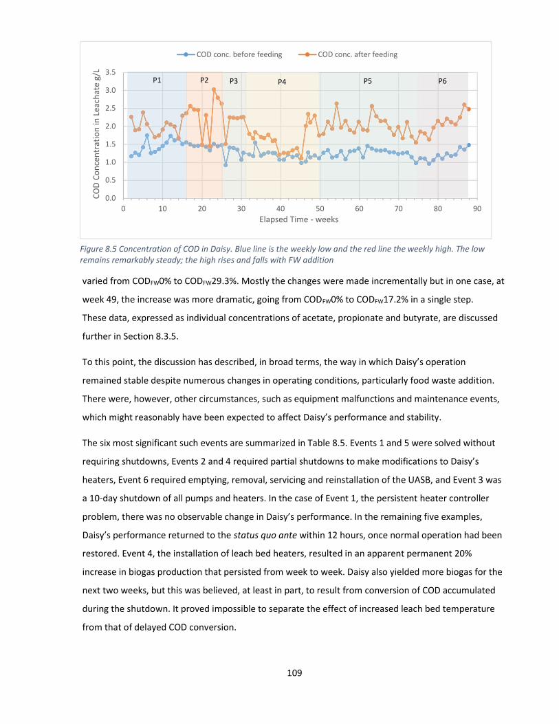
109
varied from CODFW0% to CODFW29.3%. Mostly the changes were made incrementally but in one case, at
week 49, the increase was more dramatic, going from CODFW0% to CODFW17.2% in a single step.
These data, expressed as individual concentrations of acetate, propionate and butyrate, are discussed
further in Section 8.3.5.
To this point, the discussion has described, in broad terms, the way in which Daisy’s operation
remained stable despite numerous changes in operating conditions, particularly food waste addition.
There were, however, other circumstances, such as equipment malfunctions and maintenance events,
which might reasonably have been expected to affect Daisy’s performance and stability.
The six most significant such events are summarized in Table 8.5. Events 1 and 5 were solved without
requiring shutdowns, Events 2 and 4 required partial shutdowns to make modifications to Daisy’s
heaters, Event 6 required emptying, removal, servicing and reinstallation of the UASB, and Event 3 was
a 10-day shutdown of all pumps and heaters. In the case of Event 1, the persistent heater controller
problem, there was no observable change in Daisy’s performance. In the remaining five examples,
Daisy’s performance returned to the status quo ante within 12 hours, once normal operation had been
restored. Event 4, the installation of leach bed heaters, resulted in an apparent permanent 20%
increase in biogas production that persisted from week to week. Daisy also yielded more biogas for the
next two weeks, but this was believed, at least in part, to result from conversion of COD accumulated
during the shutdown. It proved impossible to separate the effect of increased leach bed temperature
from that of delayed COD conversion.
0.0
0.5
1.0
1.5
2.0
2.5
3.0
3.5
0 10 20 30 40 50 60 70 80 90
COD
Con
cent
ratio
n in
Lea
chat
e g/
L
Elapsed Time - weeks
COD conc. before feeding COD conc. after feeding
P1 P2 P3 P4 P5 P6
Figure 8.5 Concentration of COD in Daisy. Blue line is the weekly low and the red line the weekly high. The low remains remarkably steady; the high rises and falls with FW addition

110
Throughout 83 weeks of continuous operation Daisy remained completely stable, easily
accommodating changes in feedstock and temporary process disruptions. Undoubtedly, the high C:N
ratio contributed to this, but the buffering capacity of six leach beds, each at a different stage of the
digestion process, appears to also have contributed; this will be discussed further in Section 8.4. Tank
removal and UASB removal (Events 2 and 6 respectively) were complex undertakings requiring
Table 8.5 Major Malfunctions and Maintenance Events
Dates Description Response
Impacts on stability or performance
Comments
Event Start End Potential Actual
1 2015/06/04 Week 11
2015/08/05 Week 20
TI heater repeatedly cut out; the cause was never
determined with certainty
Raised the RTD about 5cm, out of what was believed to be a cool mixing zone
lower destruction efficiency, decline in biogas production
None observed
Believed to be caused by an undisclosed failsafe circuit in the controller
2
2015/07/22 Week 18
2015/08/06 Week 20
one day event
one day
event
Tank heaters underpowered, wrong
type of heat tape
T1 heat tape replacement T2 heat tape replacement
Ingress of air, loss of biogas, impairment of microbial community
Short term loss in biogas production; made up in subsequent days
Required removal and replacement of each tank
3 2015/09/04
Week 24 2015/09/14
Week 25 Temporary shutdown of
heaters and pumps
Daisy restarted - carefully planned; within 14h all normal; gas production picked up quickly.
VFA inhibition; plugging of valves or lines; drop in destruction efficiency
observed; biogas production caught up over next two weeks
Deliberate action, partly to test the effect of shutdown and restart (partly to have a short holiday)
4 2015/09/14
Week 25 20/15/2015
Week 26 Installation of heaters on each leach bed
Removed leach beds one at a time; rest of Daisy operating
Hydraulic upset - pressure loss from removal and replacement of leach beds
None; system ran fine
Biogas production rose 20% after heaters turned on; temp rose from 35°C to 40°C
5 2016/03/09
Week 51 2016/03/10
Week 51
Hydraulic imbalance; clarifier ran dry; starved UASB; gas pumped through UASB; some granules lost to T2
Pumps to 100% for five minutes, flushed lines; palpated balance tube between T1 - T2
Loss of UASB function; hydraulic imbalance
Temporary transfer of biogas to GM1; rapid return to normal
Probably a blockage of the tank balance tube; never fully explained; no recurrence
6 2016/05/12
Week 55 2016/05/12
Week 60 UASB performance
declined;
Shut down UASB, emptied; re and re; flow distributor plugged; removed geotextile;
Permanent loss of UASB function; malfunction of balance of system
None; UASB out of service 09.00h returned to service 14.30h; back to normal 23.00h
System unperturbed by temporary absence of UASB
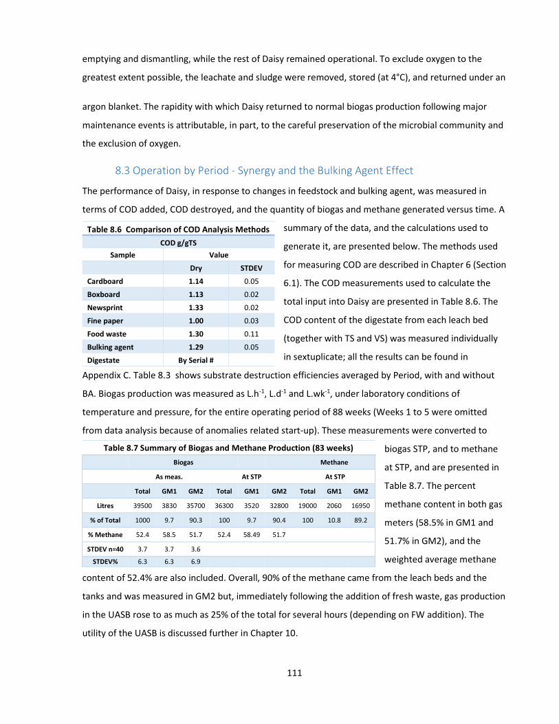
111
emptying and dismantling, while the rest of Daisy remained operational. To exclude oxygen to the
greatest extent possible, the leachate and sludge were removed, stored (at 4°C), and returned under an
argon blanket. The rapidity with which Daisy returned to normal biogas production following major
maintenance events is attributable, in part, to the careful preservation of the microbial community and
the exclusion of oxygen.
8.3 Operation by Period - Synergy and the Bulking Agent Effect
The performance of Daisy, in response to changes in feedstock and bulking agent, was measured in
terms of COD added, COD destroyed, and the quantity of biogas and methane generated versus time. A
summary of the data, and the calculations used to
generate it, are presented below. The methods used
for measuring COD are described in Chapter 6 (Section
6.1). The COD measurements used to calculate the
total input into Daisy are presented in Table 8.6. The
COD content of the digestate from each leach bed
(together with TS and VS) was measured individually
in sextuplicate; all the results can be found in
Appendix C. Table 8.3 shows substrate destruction efficiencies averaged by Period, with and without
BA. Biogas production was measured as L.h-1, L.d-1 and L.wk-1, under laboratory conditions of
temperature and pressure, for the entire operating period of 88 weeks (Weeks 1 to 5 were omitted
from data analysis because of anomalies related start-up). These measurements were converted to
biogas STP, and to methane
at STP, and are presented in
Table 8.7. The percent
methane content in both gas
meters (58.5% in GM1 and
51.7% in GM2), and the
weighted average methane
content of 52.4% are also included. Overall, 90% of the methane came from the leach beds and the
tanks and was measured in GM2 but, immediately following the addition of fresh waste, gas production
in the UASB rose to as much as 25% of the total for several hours (depending on FW addition). The
utility of the UASB is discussed further in Chapter 10.
Table 8.6 Comparison of COD Analysis Methods
COD g/gTS Sample Value
Dry STDEV
Cardboard 1.14 0.05
Boxboard 1.13 0.02
Newsprint 1.33 0.02
Fine paper 1.00 0.03
Food waste 1.30 0.11
Bulking agent 1.29 0.05
Digestate By Serial #
Table 8.7 Summary of Biogas and Methane Production (83 weeks) Biogas Methane
As meas. At STP At STP
Total GM1 GM2 Total GM1 GM2 Total GM1 GM2
Litres 39500 3830 35700 36300 3520 32800 19000 2060 16950
% of Total 1000 9.7 90.3 100 9.7 90.4 100 10.8 89.2
% Methane 52.4 58.5 51.7 52.4 58.49 51.7
STDEV n=40 3.7 3.7 3.6
STDEV% 6.3 6.3 6.9

112
The analysis of the elemental composition and ash content of all the substrates (Table 8.8) was used for
two main purposes, to calculate the C:N ratio (see Table 8.9), and to calculate the stoichiometry of the
digestion process for the average substrate, based
on the entire 83 week digestion period (Figure 8.8).
From the stoichiometric equation, the average methane content of the biogas was calculated at 52.5%
and corresponded satisfactorily with the measured value (weighted average of GM1 and GM2) of
52.4±3.7%. Table 8.10 is a complete summary of the mass balance for each operating Period.
Table 8.8 Elemental Analysis - Average of three samples
Substrate
Analest1 TKN Diosady2
TS/VS
Weight percent C H O N Ash
CB 41.3 5.96 44.1 0.17 8.55
BB 39.4 5.67 42.2 0.11 12.7
NP 46.8 6.39 45.8 0.06 0.94
FP 37.2 5.57 41.0 0.03 16.3
FW 47.7 6.92 32.4 3.04 9.97
BA 46.6 6.19 45.1 0.25 1.84 1 Department of Chemistry, 2Department of Chemical Engineering
Table 8.9 Carbon Nitrogen Ratio
CODFW% Substrate Samples Avg. STDEV
Set 1 Set 2 Set 3 n = 3
0 356 356 343 352 7.6
7.9 133 133 123 130 5.4
12.9 95.3 95.3 88.2 92.9 4.1
17.2 76.4 76.4 70.6 74.4 3.3
21.7 63.3 63.3 58.5 61.7 2.8
29.3 49.0 49.0 45.3 47.8 2.1
Substrate: from elemental analysis of FW+FB+BA, average fed to Daisy (weeks 5 – 88): C90
H155
O67
N (n=90 a=155
b=67 c=1), nitrogen source: ammonia.
d = (4n + a – 2b – 3c) = 378
fe = 1 – f
s = 1 – 0.08 = 0.92 (f
s from Rittmann and McCarty for anaerobic reactions – low biomass yield)
ra: 0.125CO
2 + H
+ + e
- = 0.125CH
4 + 0.25H
2O
rc: 0.2CO
2 + 0.05NH
4
+ + 0.05HCO
3
- + H
+ + e
- = 0.05C
5H
7O
2N + 0.45H
2O
rd: (c(n-c)/d)CO
2 + (c/d)NH
4
+ + (c/d)HCO
3
- + H
+ + e
- = (1/d)C
nH
aO
bN
c + ((2n-b+c)/d)H
2O
- rd: 0.235CO
2 + 0.00264NH
4
+ + 0.00264HCO
3
- + H
+ + e
- = 0.00264C
90H
155O
67N + 0.301H
2O
fer
a: 0.115CO
2 + 0.92H
+ + 0.92e
- = 0.115CH
4 + 0.23H
2O
fsr
c: 0.016CO
2 + 0.004NH
4
+ + 0.004HCO
3
- + 0.08H
+ + 0.08e
- = 0.004C
5H
7O
2N + 0.036H
2O
0.00264C90
H155
O67
N + 0.035H2O = 0.004C
5H
7O
2N + 0.115CH
4 + 0.104CO
2 + 0.00136NH
4
+ + 0.00136HCO
3
-
1.94C90
H155
O67
N + 25.7H2O = 2.98C
5H
7O
2N + 84.6CH
4 + 76.4CO
2 + NH
4
+ + HCO
3
-
COD content: substrate = 1.25 gCOD.gVS-1
cells = 1.42 gCOD.gVS-1
Calculated methane content: (84.6/84.6+76.4)*100 = 52.5%
Average operating methane content (weeks 5 to 88) = 52.4%
Figure 8.8 Stoichiometry of digestion of the 83 week average substrate; calculation of percent methane in biogas from first principles based on elemental analysis.

113
The mass balance calculation is a measure of the percentage of the COD destroyed that can be
accounted for by the COD in the methane generated (Equation 8.1). The numerator is the volume of
methane produced at STP converted to grams of COD at 350 mL per gram, plus the COD estimated to
have been consumed to generate new cells (collectively products). The denominator is the amount of
COD destroyed (reactants);
𝑀𝑎𝑠𝑠 𝑏𝑎𝑙𝑎𝑛𝑐𝑒 =
.
. . ( )× .
( )× 100% [8.1]
The percent mass balance between one operating period and the next varies for two reasons; firstly, at
low biogas production the calculation of substrate destruction becomes the difference between two
large numbers with its inherent uncertainty; secondly, it is difficult to match substrate destruction with
biogas production particularly during periods when digester conditions are changing. To illustrate this
second point, Table 8.11 shows a segment of the chart (Weeks 43 to 56 inclusive) of all the leach beds’
serial numbers through the duration of the research programme (the entire chart is in Appendix B). The
period between the two double red lines, Weeks 44 to 49 inclusive, is the period of the lowest biogas
production, Period 4c. Leach bed serial numbers in deep yellow, S.043 to S.048, are the leach beds to
which no food waste was added. It can readily be seen that, while those leach beds are the
Table 8.10 Mass Balance by Period Operating Data COD g
Methane Mass
balance %
Period Weeks Serial Nos. (a) Subs. in
(b) DG out
(c) Destr.
(d) Conv. Cells
(e) Conv. to CH4
Total out (g) + (d)
(f) Vol. out L.
(g) COD out g.
1 6 - 15 S.008 - S.017 20970 12710 8260 660 7600 7680 2460 7020 93.0
2 16 - 24 S.018 - S.024 14680 8920 5760 461 5300 5460 1750 5000 94.8
3 25 - 31 S.025 - S.030 14680 6240 5000 340 4600 5170 1610 4600 98.9
4a 32 - 37 S.030 - S.035 12220 8480 3740 299 3440 3770 1210 3470 100.7
4b 38 - 44 S.036 - S.042 13620 10560 3060 245 2820 3030 975 2790 98.9
4c 44 - 49 S.043 - S.048 11080 9560 1520 1228 1400 1340 428 1220 88.3
5a 50 - 57 S.049 - S.056 16770 11090 5690 4558 5230 5220 1670 4760 91.8
5b 58 - 63 S.057 - S.062 12580 8400 4180 3356 3850 4510 1460 4170 107.8
5c 64 - 70 S.063 - S.068 12580 8590 3990 319 3670 4160 1350 3840 104.3
5d 71 - 74 S.069 - S.073 10480 6520 3960 317 3640 3820 1230 3500 96.5
6a 74 - 80 S.074 - S.079 13080 7640 5440 435 5010 5410 1740 4970 99.4
6b 81 - 86 S.080 - S.087 14080 7120 6960 5578 6400 6960 2240 6400 100.0
Totals 6 - 88 S.008 - S.087 167300 108900 58390 4670 53720 58830 18960 54160 100.8
mass balance = (g+d)/c*100% c = a - b d = c*0.08 e = c - d g = f/0.35l.gCOD-1
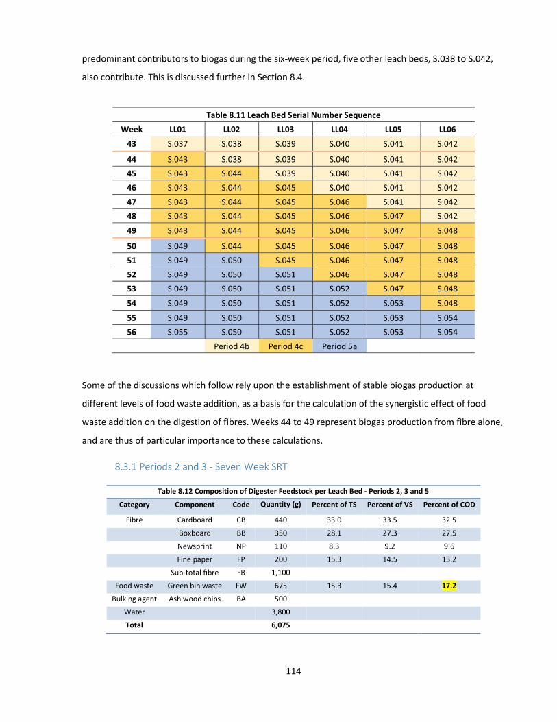
114
predominant contributors to biogas during the six-week period, five other leach beds, S.038 to S.042,
also contribute. This is discussed further in Section 8.4.
Table 8.11 Leach Bed Serial Number Sequence
Week LL01 LL02 LL03 LL04 LL05 LL06
43 S.037 S.038 S.039 S.040 S.041 S.042
44 S.043 S.038 S.039 S.040 S.041 S.042
45 S.043 S.044 S.039 S.040 S.041 S.042
46 S.043 S.044 S.045 S.040 S.041 S.042
47 S.043 S.044 S.045 S.046 S.041 S.042
48 S.043 S.044 S.045 S.046 S.047 S.042
49 S.043 S.044 S.045 S.046 S.047 S.048
50 S.049 S.044 S.045 S.046 S.047 S.048
51 S.049 S.050 S.045 S.046 S.047 S.048
52 S.049 S.050 S.051 S.046 S.047 S.048
53 S.049 S.050 S.051 S.052 S.047 S.048
54 S.049 S.050 S.051 S.052 S.053 S.048
55 S.049 S.050 S.051 S.052 S.053 S.054
56 S.055 S.050 S.051 S.052 S.053 S.054
Period 4b Period 4c Period 5a
Some of the discussions which follow rely upon the establishment of stable biogas production at
different levels of food waste addition, as a basis for the calculation of the synergistic effect of food
waste addition on the digestion of fibres. Weeks 44 to 49 represent biogas production from fibre alone,
and are thus of particular importance to these calculations.
8.3.1 Periods 2 and 3 - Seven Week SRT
Table 8.12 Composition of Digester Feedstock per Leach Bed - Periods 2, 3 and 5
Category Component Code Quantity (g)
grams
Percent of TS Percent of VS Percent of COD
Fibre Cardboard CB 440 33.0 33.5 32.5 Boxboard BB 350 28.1 27.3 27.5 Newsprint NP 110 8.3 9.2 9.6 Fine paper FP 200 15.3 14.5 13.2
Sub-total fibre FB 1,100
Food waste Green bin waste FW 675 15.3 15.4 17.2
Bulking agent Ash wood chips BA 500
Water 3,800
Total 6,075

115
The original plan was to complete two seven-week cycles in Period 2. The SRT was lengthened to seven
weeks from six by introducing a fresh leach bed each week for six weeks in a row, then skipping the
seventh. The feedstock composition during Periods 2, 3 and 5, Table 8.12, is unchanged from Period 1.
Figure 8.9 shows that biogas production in Period 2 fell to a nine-week average of 367 L.wk-1 (from 509
L.wk-1 in Period 1) a drop of 28%, but COD destruction efficiency (Table 8.3) was unchanged at 53.5%
compared to 53.7% in Period 1. Appendix D contains complete tables showing substrate destruction
efficiency, and mass balance for all 6 Periods. Essentially, the yield was the same but the digestion rate
had fallen by almost 30%; nothing could be gained from a longer SRT. The elimination of a fresh leach
bed every seven weeks made biogas production uneven, hence the dips at Week 16 and Week 23. The
experiment was terminated after 9 weeks at Week 25, and Period 3 was begun by returning Daisy to a
six week SRT; no other changes were made.
The more pronounced drop in biogas production at Week 25 was the result of a 10 - day shutdown of
pumps and heaters. This was to accommodate a short vacation but also to test robustness and stability
on restart; the restart went smoothly with a rapid return to normal operation. The purpose of Period 3
was simply to re-establish stable biogas production with a six week SRT as a starting point from which
to begin the next experiment. As Figure 8.10 shows, biogas production rose to more than 600 L.wk-1,
about 100 L.wk-1 greater than Period 1, despite the identical operating conditions.
0
100
200
300
400
500
600
15 17 19 21 23 25
Biog
as p
rodu
ctio
n L/
wk
at 2
97K
Elapsed Time - weeks
Total GM1 GM2
Period 2 - 7 week SRT
Figure 8.9 Weekly biogas production – Period 2; 7 wk. SRT; LB6 replacement postponed one week at wk. 16 and at wk. 23 to create 7wk. cycle; beginning of short shutdown at wk. 25
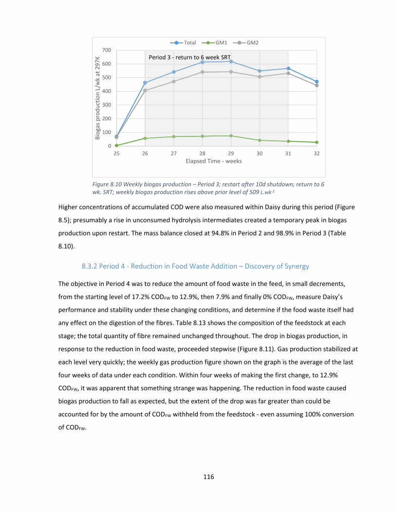
116
Higher concentrations of accumulated COD were also measured within Daisy during this period (Figure
8.5); presumably a rise in unconsumed hydrolysis intermediates created a temporary peak in biogas
production upon restart. The mass balance closed at 94.8% in Period 2 and 98.9% in Period 3 (Table
8.10).
8.3.2 Period 4 - Reduction in Food Waste Addition – Discovery of Synergy
The objective in Period 4 was to reduce the amount of food waste in the feed, in small decrements,
from the starting level of 17.2% CODFW to 12.9%, then 7.9% and finally 0% CODFW, measure Daisy’s
performance and stability under these changing conditions, and determine if the food waste itself had
any effect on the digestion of the fibres. Table 8.13 shows the composition of the feedstock at each
stage; the total quantity of fibre remained unchanged throughout. The drop in biogas production, in
response to the reduction in food waste, proceeded stepwise (Figure 8.11). Gas production stabilized at
each level very quickly; the weekly gas production figure shown on the graph is the average of the last
four weeks of data under each condition. Within four weeks of making the first change, to 12.9%
CODFW, it was apparent that something strange was happening. The reduction in food waste caused
biogas production to fall as expected, but the extent of the drop was far greater than could be
accounted for by the amount of CODFW withheld from the feedstock - even assuming 100% conversion
of CODFW.
0
100
200
300
400
500
600
700
25 26 27 28 29 30 31 32
Biog
as p
rodu
ctio
n L/
wk
at 2
97K
Elapsed Time - weeks
Total GM1 GM2
Period 3 - return to 6 week SRT
Figure 8.10 Weekly biogas production – Period 3; restart after 10d shutdown; return to 6 wk. SRT; weekly biogas production rises above prior level of 509 L.wk-1

117
For example, at the first plateau (CODFW12.9%), biogas production should have been no less than 462
L.wk-1 if the reduction in food waste alone was responsible, instead it was 414 L.wk-1. By the time food
waste addition had been reduced to zero, the discrepancy had grown to almost 200 L.wk-1 of biogas (at
297K); in other words, almost 40% of the biogas produced at CODFW17.2% where the experiment
began, could not be properly accounted for. Substrate destruction efficiency, on a COD basis, fell with
each reduction in food waste, to 38.9% then 31.8% and finally to 18.6% at CODFW0% (Table 8.3). A
leachate analysis confirmed that unconverted COD was not accumulating within Daisy, so what was
happening?
Table 8.13 Composition of Digester Feedstock per Leach Bed– Periods 4a, 4b and 4c
Category Component Code Quantity (g) Percent of TS Percent of VS Percent of COD Fibre Cardboard CB 440 Boxboard BB 350 Newsprint NP 110 Fine paper FP 200 Sub-total fibre FB 1,100 Bulking agent Ash wood chips BA 500 Food waste Green bin waste FW 480 11.4 11.4 12.9 Water 3,800 Total 4a 5,880
Food waste Green bin waste FW 280 7.0 7.0 7.9 Water 3,800 Total 4b 5,680 Food waste Green bin waste FW 0 0.0 0.0 0.0
Water 3,800 Total 4c 5,400
0
100
200
300
400
500
600
30 35 40 45 50
Biog
as p
rodu
ctio
n L/
wk
at 2
97K
Elapsed Time - weeks
Total GM1 GM2
Period 4 - FW reduction to zero in 3 steps
414L/wk.
287L/wk.
132L/wk.
Figure 8.11 Weekly Biogas Production – Period 4: FW to zero in 3 steps; stable biogas production established at each level. Biogas drop greater than explicable by reduction in FW.

118
The initial, tentative, conclusion was that an unexpectedly large synergistic effect, created by adding
food waste, was significantly enhancing the digestibility of the fibres and was related in some way to
the amount of food waste added. The implications for process design (SRT in particular) prompted a
mid-course correction. Four steps were decided upon.
a) The literature was revisited to see if this behaviour had been reported. I was unable to find
any references to a synergistic effect on the digestion of wood-derived lignocellulosic fibres
with the help of food waste.
b) A simple calculation to measure synergy was devised, based upon two assumptions; firstly,
that fibre alone produced 122 L.wk-1 of biogas at STP (132 L.wk-1 as-measured); secondly,
that the total amount of biogas produced without synergy could not exceed the sum of 122
L.wk-1 plus the food waste contribution calculated at 100% COD conversion. Thus the
synergy could be calculated as follows:
𝑉 . 𝑉 − 𝑉 − 𝑉 [8.2]
I subsequently found a reference to a synergistic effect of food waste addition on the
digestion of waste activated sludge, in which this same calculation was used to measure
synergy (Yun et al., 2015).
c) The plan for BMP 2 was modified and expanded, specifically to study synergy; the results
are presented in Chapter 9. BMP 3, digesting larger quantities of substrate under conditions
similar to Daisy’s is also presented in Chapter 9.
d) The experimental programme was revised to concentrate on quantifying the apparent
synergistic effect of food waste within Daisy. In Period 5 Daisy was returned to CODFW17.2%
in a single step, firstly to test stability under more extreme changes, and secondly to re-
establish a stable baseline of biogas production from which to explore synergy at higher
levels of food waste addition.
The mass balance closed at 100.7% in Period 4a, 98.9% in Period 4b and 88.3% in Period 4c.
8.3.3 Period 5 – Raising Food Waste Addition; the Bulking Agent Effect
The plan for Period 5 was to raise CODFW to 17.2% in one step and return Daisy to stable biogas
production, presumably at just over 500 L.wk-1 based on Period 1, and to test Daisy’s stability under this
more abrupt change in food waste addition.

119
The assumption was that this would take 8 to 10 weeks. From Week 59 to Week 56, everything went as
planned, but at Week 56 gas production took a sharp upturn and rose to just under 600 L.wk-1. By this
point, supplies of the fourth bulking agent shipment, BA4, were running low so at Week 58 Daisy was
switched to BA5 (see Figure 8.12).
Bulking agent is used for the specific purpose of maintaining the permeability and structure of the
waste mass in the leach beds for the six weeks of SRT. Of the materials fed to Daisy, BA is the only one
that varied substantially in its properties during the course of the research programme. It always took
the form of ground up ash wood and was supplied by Miller Waste Systems as part of their in-kind
contribution to the project. In all, six batches were delivered over the entire duration of the
experiment; Batches BA1, BA2, BA4 and BA6 were ground in a Roto-chopper and screened, Batch 3 was
ground in a Peterson Grinder, and BA5 was ground by an independent tree company who used a
chipper. Batches BA1, BA2, and BA4 worked well in the sense that switching from one to another
caused no noticeable changes in Daisy’s performance; Batch 3 was rejected because the particle size
was far too coarse.
BA5 had a different physical appearance; it was coarser, shorter and fatter. It was first used at the
beginning of Week 58, one week after gas production had returned to prior levels, and used for six
0
100
200
300
400
500
600
700
49 54 59 64 69 74
Biog
as p
rodu
ctio
n L/
wk
at 2
97K
Elapsed Time - weeks
Total GM1 GM2
BA4 BA5 BA4 BA6
513L/wk.
Figure 8.12 Weekly biogas production – Period 5; return to CODFW17.2%; properties of BA5 apparently lowering biogas yield and substrate destruction efficiency
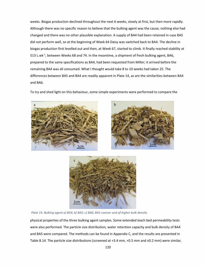
120
weeks. Biogas production declined throughout the next 6 weeks, slowly at first, but then more rapidly.
Although there was no specific reason to believe that the bulking agent was the cause, nothing else had
changed and there was no other plausible explanation. A supply of BA4 had been retained in case BA5
did not perform well, so at the beginning of Week 64 Daisy was switched back to BA4. The decline in
biogas production first levelled out and then, at Week 67, started to climb. It finally reached stability at
513 L.wk-1, between Weeks 68 and 74. In the meantime, a shipment of fresh bulking agent, BA6,
prepared to the same specifications as BA4, had been requested from Miller; it arrived before the
remaining BA4 was all consumed. What I thought would take 8 to 10 weeks had taken 25. The
differences between BA5 and BA4 are readily apparent in Plate 14, as are the similarities between BA4
and BA6.
To try and shed light on this behaviour, some simple experiments were performed to compare the
physical properties of the three bulking agent samples. Some extended leach bed permeability tests
were also performed. The particle size distribution, water retention capacity and bulk density of BA4
and BA5 were compared. The methods can be found in Appendix C, and the results are presented in
Table 8.14. The particle size distributions (screened at +3.4 mm, +0.5 mm and ±0.2 mm) were similar,
a
1cm 1cm
b
1cm
c
Plate 14. Bulking agent a) BA4; b) BA5; c) BA6; BA5 coarser and of higher bulk density

121
though BA5 had a higher proportion of coarse material, however their bulk densities were very
different, 0.12 kg.l-1 for BA4 vs. 0.22 kg.l-1 for BA5, and BA4 had a greater water retention capacity. The
morphology of the two batches was also quite different. BA4 consisted of longer, finer, pieces of wood
which may serve to enhance lateral movement of leachate in the leach beds.
The substrate destruction efficiency
reflected the trends in biogas production.
During Period 5a destruction efficiency rose
sharply to 51.7%, from 18.6%, then fell to
43.8% and 43.9% in Periods 5b and 5c
respectively. Finally, in period 5d, it rose to
53.0%, reestablishing the performance of
Periods 1, 2 and 3. An extended series of
leach bed permeability tests was conducted,
using a procedure similar to that described in Chapter 7 (Section 7.1). Leachate (565mL) was delivered
automatically by P3 at 510 mL/min. and the drainage rate of leachate measured until 520 mL had been
recovered. These tests were planned and conducted in the hope that they would make it possible to
distinguish between the behaviour of leach beds with BA4 from those with BA5 (and ultimately BA6) in
a way that might explain the drop in biogas production and digestion efficiency during this period.
Unfortunately, no clear pattern emerged, and no correlation between leach bed drainage properties
and substrate destruction or biogas production was found. A subset of the data is provided in Appendix
D, and the entire data set in EDF6. This finding was contrary to the earlier permeability tests, which had
confirmed that BA2, which was very coarse, did indeed show different drainage behaviour; perhaps, in
the case of BA5 vs. BA4, the difference was too subtle. The mass balance closed at 91.8% in Period 5a,
107.8% in Period 5b, 104.3% in Period 5c and 96.5% in Period 5d. Despite the unexpected behaviour
biogas production and substrate destruction ultimately returned to previous levels, and no process
instability was observed during this period. It still seems most probable that the changes in BA both
caused, and rectified, this anomalous behaviour. The answer may lie in the moisture retention
properties of the BA and this is discussed further in Chapter 10.
8.3.4 Period 6 - High Levels of Food Waste Addition
The final step was to increase food waste addition further, to test the effect on synergy and on Daisy’s
stability. In Period 6a, CODFW was raised to 21.7% and in Period 6b to 29.3%. Biogas production levelled
off at 620 L.wk-1 at CODFW21.7% and 797 L.wk-1 at CODFW29.3% (at 297K) as shown in Figure 8.13. Of
this amount, 244 L.wk-1 and 300 L.wk-1 respectively (at 297K) were attributable to synergistic digestion
Table 8.14 Physical Properties of Bulking Agents BA4 and BA5
Particle Size Distribution %
>3.36mm <3.36mm>0.50mm <0.50mm>0.21mm <0.21mm
BA4 44.7 37.9 12.5 3.4
BA5 52.8 31.2 11.7 2.9
Water Retention gH2O/gBA
BA4 2.95
BA5 2.33
Bulk Density kg/L
BA4 0.119
BA5 0.220
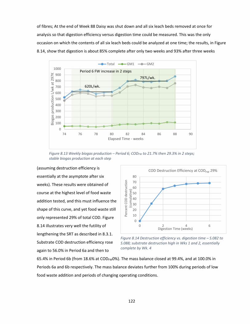
122
of fibres; At the end of Week 88 Daisy was shut down and all six leach beds removed at once for
analysis so that digestion efficiency versus digestion time could be measured. This was the only
occasion on which the contents of all six leach beds could be analyzed at one time; the results, in Figure
8.14, show that digestion is about 85% complete after only two weeks and 93% after three weeks
(assuming destruction efficiency is
essentially at the asymptote after six
weeks). These results were obtained of
course at the highest level of food waste
addition tested, and this must influence the
shape of this curve, and yet food waste still
only represented 29% of total COD. Figure
8.14 illustrates very well the futility of
lengthening the SRT as described in 8.3.1.
Substrate COD destruction efficiency rose
again to 56.0% in Period 6a and then to
65.4% in Period 6b (from 18.6% at CODFW0%). The mass balance closed at 99.4%, and at 100.0% in
Periods 6a and 6b respectively. The mass balance deviates further from 100% during periods of low
food waste addition and periods of changing operating conditions.
0
100
200
300
400
500
600
700
800
900
1000
74 76 78 80 82 84 86 88 90
Biog
as p
rodu
ctio
n L/
wk
at 2
97K
Elapsed Time - weeks
Total GM1 GM2
Period 6 FW increase in 2 steps
620L/wk.
797L/wk.
Figure 8.13 Weekly biogas production – Period 6; CODFW to 21.7% then 29.3% in 2 steps; stable biogas production at each step
01020304050607080
0 2 4 6
Perc
ent C
OD
des
truc
tion
(cum
ulat
ive)
Digestion Time (weeks)
COD Destruction Efficiency at CODFW 29%
Figure 8.14 Destruction efficiency vs. digestion time – S.082 to S.088; substrate destruction high in Wks 1 and 2, essentially complete by Wk. 4

123
8.3.5 Synergy
Using the simple calculation described earlier, synergy was quantified, converted to STP, and the results
summarized in Table 8.15. The input to Daisy is expressed in grams of COD added per week as food
waste, and as fibre. The latter remains constant throughout. Food waste COD is then expressed as a
percentage of the total. The biogas produced is presented in litres per week at STP as four numbers, the
total, the portion attributable to food waste at 100% COD conversion, the portion attributable to
fibre alone (the difference between total and food waste), and the portion attributable to synergy (the
difference between fibre total and fibre at zero food waste addition). Specific biogas is expressed as
L.kg-1 CODadded. The results are
displayed graphically in Figures
8.15, 8.16 and 8.17.The growth in
synergistic biogas with increasing
food waste addition is clearly
evident. At CODFW29.3%, the biogas
generated from fibre was 325% of
that generated from the same
amount of fibre at CODFW0%. The
foundation for these calculations is
the measurement of 122 L.wk-1 of
biogas (at STP) from fibre alone;
how reliable is this number? Is it
trustworthy? While it would have been preferable to operate at CODFW0% for a more prolonged period,
it is unlikely that gas production would have risen, but it may have gone lower with time. The value for
Table 8.15 Calculation of Synergy at 100% FW conversion
CODIN (per week) Biogas Production (L.wk-1 at STP) Specific Production L.kg-1 CODadded
FW ST
DEV FB Total FW
ST
DEV
Total meas
ST DEV
n FW FB FB
w/o syn.
Syn. FW FB Total Syn. STDEV
g g g % n = 27
0 0.0 1,200 1,200 0.0 0.0 122 7.7 4 0 122 122 0 0 101 101 0 6.4
104 8.7 1,200 1,310 7.9 0.1 264 6.4 4 69 195 122 73 53 162 202 61 4.9
178 15.0 1,200 1,380 12.9 0.1 379 11.4 4 119 261 122 139 86 217 275 115 8.2
250 21.0 1,200 1,450 17.2 0.2 468 23.1 16 167 302 122 180 115 250 322 149 15.9
333 28.1 1,200 1,540 21.7 0.4 569 21.1 6 223 346 122 224 145 288 370 186 13.7
500 42.1 1,200 1,700 29.3 0.7 731 13.7 6 334 397 122 275 196 330 429 229 8.1
0
100
200
300
400
500
600
700
800
0.0 7.9 12.9 17.2 21.7 29.3
Biog
as -
Litr
es/w
k (a
t STP
)
Percent CODFW
Synergisticbiogasfrom fibre
Foodwaste at100% CODconversion
Fibre alone
n = 4
n = 4
n = 4
n = 16
n = 6
n = 6FW at 100% conversion
Figure 8.15 Synergistic biogas production from FB vs. FW addition; 𝑉 . 𝑉 − 𝑉 − 𝑉

124
the plateau in biogas production is the
average of four measurements over four
weeks with a standard deviation of only
6.2% (Table 8.4); this supports the
conclusion that the figure for biogas
production at CODFW0% is dependable.
Figure 8.16 shows a strong linear
relationship between synergistic biogas
production and CODFW addition. Figure
8.17 presents the same results differently,
on the basis of specific biogas production
per kgCODFWadded. Despite their linearity, this relationship must eventually change and the synergistic
effect must decline as the digestible portion of the fibres becomes consumed. The results make a
strong and persuasive case for a powerful synergistic effect in the anaerobic digestion of lignocellulosic
fibres, resulting from the addition of food waste to wood-based lignocellulosic fibres. Furthermore,
they show that the relationship between
the amount of FW added and synergistic
biogas produced is almost linear. But they
also raise a number of questions; what is
the mechanism at work; is the combination
of substrates the sole cause, or does the
reactor design contribute; are all the fibres
affected in the same way, or is there a
difference among them; is it a rate effect as
well as a yield effect and at what level of
FW addition does synergy reach a plateau?
Daisy’s coupon data provide some of the
answers, and the BMP experiments and the enzyme assays described in Chapter 9 provide additional
insight. The coupon results represent substrate digestibility, at 42 days, at different levels of FW
addition. They are subject to inaccuracies; the samples are small, ranging from 1.3 to 6.5 g (depending
on the substrate density) and exposure to the same digestion conditions in Daisy cannot be
guaranteed. Nevertheless, the large number of samples, a total of 277 fibre coupons and 27 bulking
agent coupons, have made it possible to calculate decent average values. The coupon data led to three
y = 8.04x + 4.033R² = 0.99
0
50
100
150
200
250
300
0 10 20 30 40
Biog
as -
Litr
es/k
gCO
Dad
ded
(at S
TP)
Percent CODtotal as FW
FW at 100% conversion.
For all x axis values n = 27
n = 4
n = 4
n = 16
n = 6
n = 6
Figure 8.17 Specific Synergistic biogas production in L.kg-1VSadded calculated at 100% FW conv.
y = 9.68x + 4.85R² = 0.99
0
50
100
150
200
250
300
350
0.0 10.0 20.0 30.0 40.0Syne
rgist
ic B
ioga
s -Li
tres
/wk
(at S
TP)
Percent CODFW
FW at 100% conversion
n = 6
n = 6
n = 4
n = 16
n = 4
Figure 8.16 Synergistic biogas production vs FW addition; L.wk-1
calculated at 100% FW conversion.
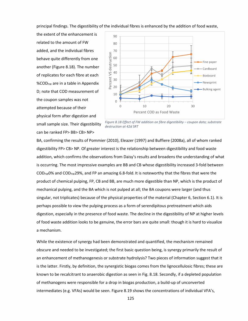
125
principal findings. The digestibility of the individual fibres is enhanced by the addition of food waste,
the extent of the enhancement is
related to the amount of FW
added, and the individual fibres
behave quite differently from one
another (Figure 8.18). The number
of replicates for each fibre at each
%CODFW are in a table in Appendix
D; note that COD measurement of
the coupon samples was not
attempted because of their
physical form after digestion and
small sample size. Their digestibility
can be ranked FP> BB> CB> NP>
BA, confirming the results of Pommier (2010), Eleazer (1997) and Buffiere (2008a), all of whom ranked
digestibility FP> CB> NP. Of greater interest is the relationship between digestibility and food waste
addition, which confirms the observations from Daisy’s results and broadens the understanding of what
is occurring. The most impressive examples are BB and CB whose digestibility increased 3-fold between
CODFW0% and CODFW29%, and FP an amazing 6.8-fold. It is noteworthy that the fibres that were the
product of chemical pulping, FP, CB and BB, are much more digestible than NP, which is the product of
mechanical pulping, and the BA which is not pulped at all; the BA coupons were larger (and thus
singular, not triplicates) because of the physical properties of the material (Chapter 6, Section 6.1). It is
perhaps possible to view the pulping process as a form of serendipitous pretreatment which aids
digestion, especially in the presence of food waste. The decline in the digestibility of NP at higher levels
of food waste addition looks to be genuine, the error bars are quite small: though it is hard to visualize
a mechanism.
While the existence of synergy had been demonstrated and quantified, the mechanism remained
obscure and needed to be investigated; the first basic question being, is synergy primarily the result of
an enhancement of methanogenesis or substrate hydrolysis? Two pieces of information suggest that it
is the latter. Firstly, by definition, the synergistic biogas comes from the lignocellulosic fibres; these are
known to be recalcitrant to anaerobic digestion as seen in Fig. 8.18. Secondly, if a depleted population
of methanogens were responsible for a drop in biogas production, a build-up of unconverted
intermediates (e.g. VFAs) would be seen. Figure 8.19 shows the concentrations of individual VFA’s,
Figure 8.18 Effect of FW addition on fibre digestibility – coupon data; substrate destruction at 42d SRT
0
10
20
30
40
50
60
70
80
90
0 10 20 30Pe
rcen
t VS
dest
ruct
ion
Percent COD as Food Waste
Fine paper
Cardboard
Boxboard
Newsprint
Bulking agent
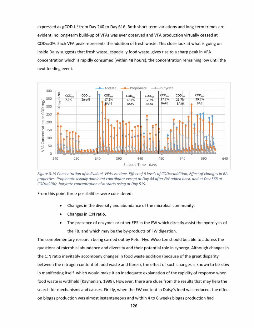
126
expressed as gCOD.L-1 from Day 240 to Day 616. Both short-term variations and long-term trends are
evident; no long-term build-up of VFAs was ever observed and VFA production virtually ceased at
CODFW0%. Each VFA peak represents the addition of fresh waste. This close look at what is going on
inside Daisy suggests that fresh waste, especially food waste, gives rise to a sharp peak in VFA
concentration which is rapidly consumed (within 48 hours), the concentration remaining low until the
next feeding event.
From this point three possibilities were considered:
Changes in the diversity and abundance of the microbial community.
Changes in C:N ratio.
The presence of enzymes or other EPS in the FW which directly assist the hydrolysis of
the FB, and which may be the by-products of FW digestion.
The complementary research being carried out by Peter HyunWoo Lee should be able to address the
questions of microbial abundance and diversity and their potential role in synergy. Although changes in
the C:N ratio inevitably accompany changes in food waste addition (because of the great disparity
between the nitrogen content of food waste and fibres), the effect of such changes is known to be slow
in manifesting itself which would make it an inadequate explanation of the rapidity of response when
food waste is withheld (Kayhanian, 1999). However, there are clues from the results that may help the
search for mechanisms and causes. Firstly, when the FW content in Daisy’s feed was reduced, the effect
on biogas production was almost instantaneous and within 4 to 6 weeks biogas production had
0
50
100
150
200
250
300
350
400
240 290 340 390 440 490 540 590 640
VFA
Conc
entr
atio
n as
CO
D m
g/L
Elapsed Time - days
Acetate Propionate Butyrate
COD
FW 1
2.9% CODFW
7.9%CODFW Zero%
CODFW 17.2%BA#5
CODFW 17.2%BA#4
CODFW17.2%BA#6
CODFW 17.2%BA#4
CODFW 29.3%BA6
CODFW 21.7% BA#6
Figure 8.19 Concentration of individual VFAs vs. time. Effect of 6 levels of CODFW addition; Effect of changes in BA properties. Propionate usually dominant contributor except at Day 44 after FW added back, and at Day 568 at CODFW29%; butyrate concentration also starts rising at Day 519.
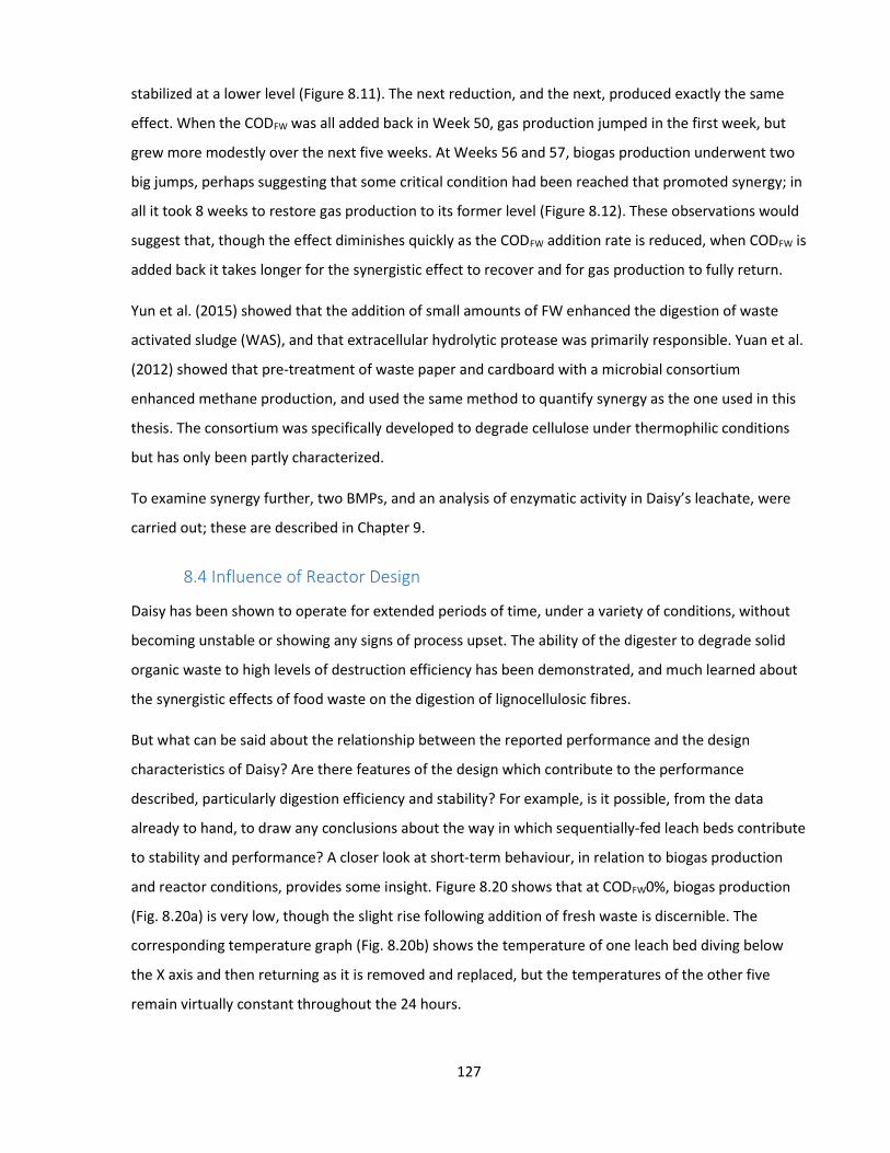
127
stabilized at a lower level (Figure 8.11). The next reduction, and the next, produced exactly the same
effect. When the CODFW was all added back in Week 50, gas production jumped in the first week, but
grew more modestly over the next five weeks. At Weeks 56 and 57, biogas production underwent two
big jumps, perhaps suggesting that some critical condition had been reached that promoted synergy; in
all it took 8 weeks to restore gas production to its former level (Figure 8.12). These observations would
suggest that, though the effect diminishes quickly as the CODFW addition rate is reduced, when CODFW is
added back it takes longer for the synergistic effect to recover and for gas production to fully return.
Yun et al. (2015) showed that the addition of small amounts of FW enhanced the digestion of waste
activated sludge (WAS), and that extracellular hydrolytic protease was primarily responsible. Yuan et al.
(2012) showed that pre-treatment of waste paper and cardboard with a microbial consortium
enhanced methane production, and used the same method to quantify synergy as the one used in this
thesis. The consortium was specifically developed to degrade cellulose under thermophilic conditions
but has only been partly characterized.
To examine synergy further, two BMPs, and an analysis of enzymatic activity in Daisy’s leachate, were
carried out; these are described in Chapter 9.
8.4 Influence of Reactor Design
Daisy has been shown to operate for extended periods of time, under a variety of conditions, without
becoming unstable or showing any signs of process upset. The ability of the digester to degrade solid
organic waste to high levels of destruction efficiency has been demonstrated, and much learned about
the synergistic effects of food waste on the digestion of lignocellulosic fibres.
But what can be said about the relationship between the reported performance and the design
characteristics of Daisy? Are there features of the design which contribute to the performance
described, particularly digestion efficiency and stability? For example, is it possible, from the data
already to hand, to draw any conclusions about the way in which sequentially-fed leach beds contribute
to stability and performance? A closer look at short-term behaviour, in relation to biogas production
and reactor conditions, provides some insight. Figure 8.20 shows that at CODFW0%, biogas production
(Fig. 8.20a) is very low, though the slight rise following addition of fresh waste is discernible. The
corresponding temperature graph (Fig. 8.20b) shows the temperature of one leach bed diving below
the X axis and then returning as it is removed and replaced, but the temperatures of the other five
remain virtually constant throughout the 24 hours.
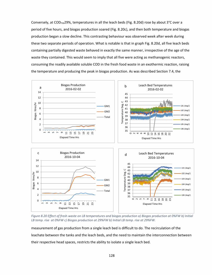
128
Conversely, at CODFW29%, temperatures in all the leach beds (Fig. 8.20d) rose by about 3°C over a
period of five hours, and biogas production soared (Fig. 8.20c), and then both temperature and biogas
production began a slow decline. This contrasting behaviour was observed week after week during
these two separate periods of operation. What is notable is that in graph Fig. 8.20d, all five leach beds
containing partially digested waste behaved in exactly the same manner, irrespective of the age of the
waste they contained. This would seem to imply that all five were acting as methanogenic reactors,
consuming the readily available soluble COD in the fresh food waste in an exothermic reaction, raising
the temperature and producing the peak in biogas production. As was described Section 7.4, the
measurement of gas production from a single leach bed is difficult to do. The recirculation of the
leachate between the tanks and the leach beds, and the need to maintain the interconnection between
their respective head spaces, restricts the ability to isolate a single leach bed.
3536373839404142434445
0 2 5 7 9 11 14 16 18 20 23
Tem
pera
ture
Deg
. C
Elapsed Time Hrs
Leach Bed Temperatures2016-10-04
LB1 (degC)
LB2 (degC)
LB3 (degC)
LB4 (degC)
LB5 (degC)
LB6 (degC)
d
0
2
4
6
8
10
12
14
1 3 5 7 9 11 13 15 17 19 21 23
Biog
as l
itres
/hr
Elapsed Time Hrs
Biogas Production2016-02-02
GM1
GM2
Total
a
0
2
4
6
8
10
12
14
1 3 5 7 9 11 13 15 17 19 21 23
Biog
as l
itres
/hr
Elapsed Time Hrs
Biogas Production2016-10-04
GM1
GM2
Total
c
3536373839404142434445
0 2 4 6 8 10 12 14 16 18 20 22
Tem
pera
ture
Deg
. C
Elapsed Time Hrs
Leach Bed Temperatures2016-02-02
LB1 (degC)
LB2 (degC)
LB3 (degC)
LB4 (degC)
LB5 (degC)
LB6 (degC)
b
Figure 8.20 Effect of fresh waste on LB temperatures and biogas production a) Biogas production at 0%FW b) Initial LB temp. rise at 0%FW c) Biogas production at 29%FW b) Initial LB temp. rise at 29%FW.

129
A method was devised that made it possible to make this measurement while still maintaining leachate
recirculation. Unfortunately, at lower rates of gas production, the measurement was very inaccurate. A
second method, in which the leach bed in question was completely isolated from the rest of Daisy
(other than its connection to GM1) for a period of four or five hours, was developed. Gas production
from a single leach bed was measured seven times over a three-week period. The results are shown in
Figure 8.21. The first measurement was made
when the waste was three days old. In the next two
measurements gas production continued to rise
and then began a decline, ending at 180 mL per
hour at Day 42. Two things are notable; firstly, the
biogas production peak, at Day 10, did not
correspond to the immediate peak shown in Figure
8.16c, suggesting that peak biogas production in
the system (first day following leach bed
replacement) does not coincide with that of an
individual fresh leach bed (Day 10 following
installation). Secondly, even a six-week old leach bed is still producing 4 or 5 L per day of biogas which
suggests that, while the substrate it contains may be spent (Figure 8.14), it may still be serving as a
reservoir for methanogens and a continuing source of biogas.
Combining all of this information, I concluded that there is a persuasive case to be made that leach
beds containing older waste serve as methanogenic reactors to consume the high concentrations of
COD, particularly VFAs, which occur immediately after fresh food waste is added and thus the design
contributes to process stability. The other related aspect of a design consisting of sequentially-fed leach
beds, is that the system is very hard to shock because not more than 16% of the contents are changed
at any one time. The other 84% therefore, by definition, serves as a buffer. This also raises the question
of the utility of the UASB and whether or not it can be eliminated. It does most of its work immediately
after Daisy is fed, during which time the UASB produces up to 25% of the biogas generated, as
measured by GM1, compared to its long-term average of 10%. Only a comparative experiment, with
and without the UASB, can answer this question definitively. Finally, Figure 8.22 consists of six graphs,
each representing a six-week period of biogas production, one for each level of food waste addition
from CODFW0% to CODFW29.3%. These graphs provide a summary of biogas production at all levels of
FW addition tested. The stability and consistency of Daisy’s operation, and response to changing food
waste addition rates, are apparent.
0
100
200
300
400
500
600
700
800
900
0 10 20 30 40 50Biog
as g
ener
atio
n ra
te m
l/h (2
97K)
Digestion Time - Days
Figure 8.21 Biogas production from a single leach bed vs. digestion time; peak at 10d does not correspond with fresh waste addition
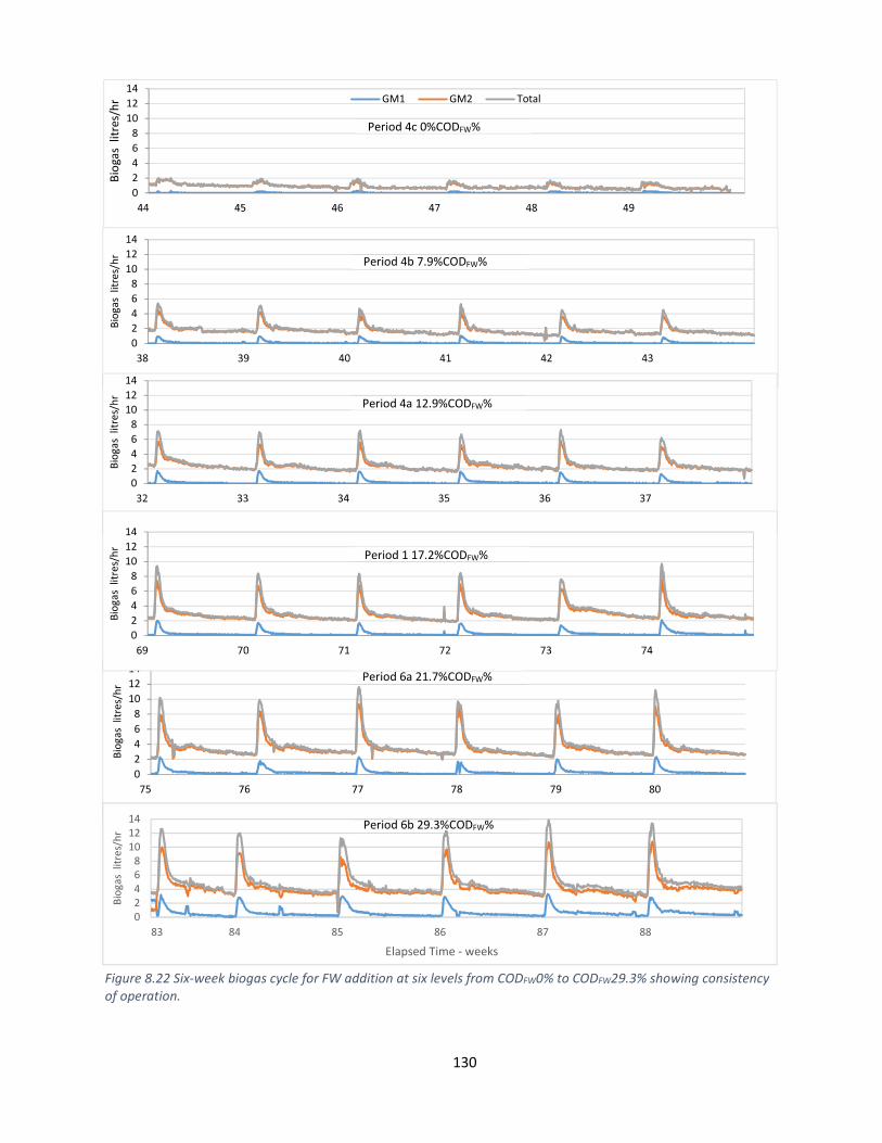
130
02468
101214
Biog
as l
itres
/hr
02468
101214
Biog
as l
itres
/hr GM1 GM2 Total
02468
101214
Biog
as l
itres
/hr
02468
101214
Biog
as l
itres
/hr
02468
101214
Biog
as l
itres
/hr
02468
101214
Biog
as l
itres
/hr
Elapsed Time - weeks
Period 6b 29.3%CODFW%
Period 6a 21.7%CODFW%
Period 1 17.2%CODFW%
Period 4a 12.9%CODFW%
Period 4b 7.9%CODFW%
Figure 8.22 Six-week biogas cycle for FW addition at six levels from CODFW0% to CODFW29.3% showing consistency of operation.
Period 4c 0%CODFW%
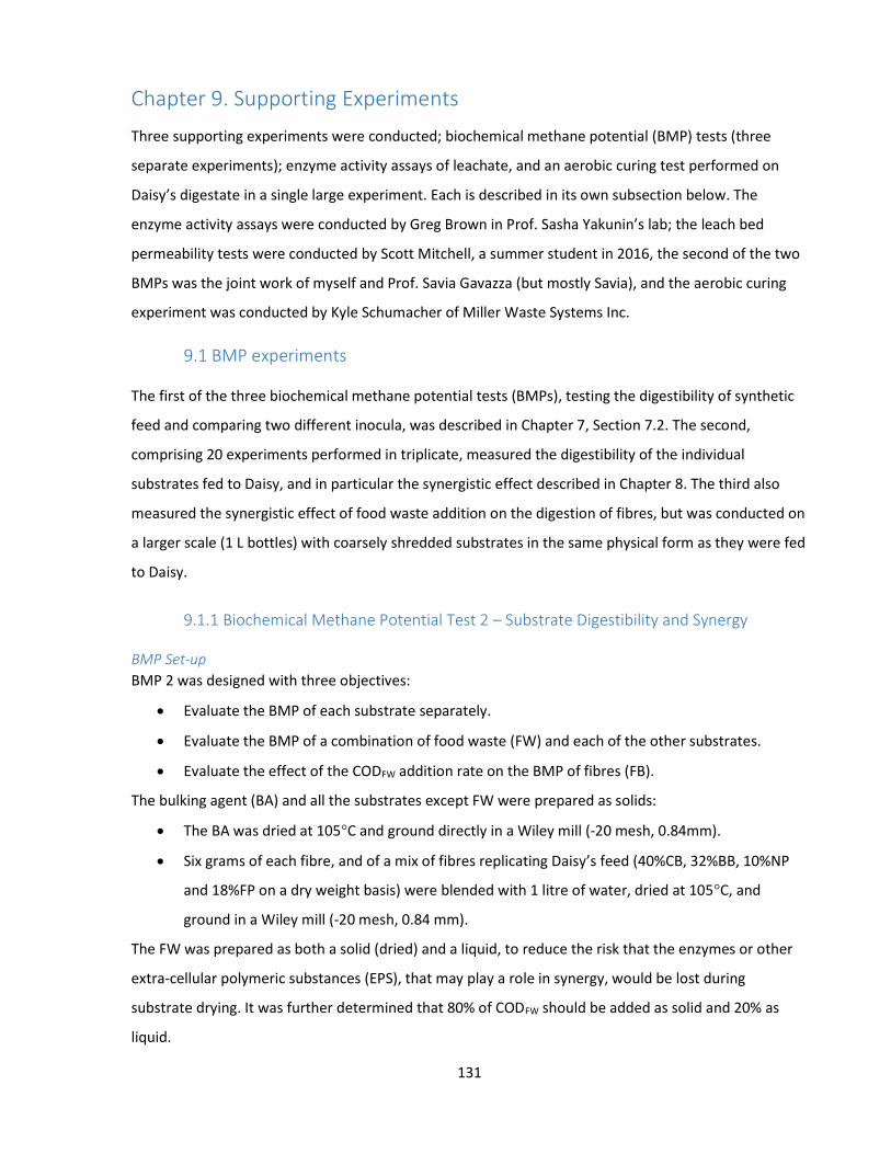
131
Chapter 9. Supporting Experiments
Three supporting experiments were conducted; biochemical methane potential (BMP) tests (three
separate experiments); enzyme activity assays of leachate, and an aerobic curing test performed on
Daisy’s digestate in a single large experiment. Each is described in its own subsection below. The
enzyme activity assays were conducted by Greg Brown in Prof. Sasha Yakunin’s lab; the leach bed
permeability tests were conducted by Scott Mitchell, a summer student in 2016, the second of the two
BMPs was the joint work of myself and Prof. Savia Gavazza (but mostly Savia), and the aerobic curing
experiment was conducted by Kyle Schumacher of Miller Waste Systems Inc.
9.1 BMP experiments
The first of the three biochemical methane potential tests (BMPs), testing the digestibility of synthetic
feed and comparing two different inocula, was described in Chapter 7, Section 7.2. The second,
comprising 20 experiments performed in triplicate, measured the digestibility of the individual
substrates fed to Daisy, and in particular the synergistic effect described in Chapter 8. The third also
measured the synergistic effect of food waste addition on the digestion of fibres, but was conducted on
a larger scale (1 L bottles) with coarsely shredded substrates in the same physical form as they were fed
to Daisy.
9.1.1 Biochemical Methane Potential Test 2 – Substrate Digestibility and Synergy
BMP Set-up BMP 2 was designed with three objectives:
Evaluate the BMP of each substrate separately.
Evaluate the BMP of a combination of food waste (FW) and each of the other substrates.
Evaluate the effect of the CODFW addition rate on the BMP of fibres (FB).
The bulking agent (BA) and all the substrates except FW were prepared as solids:
The BA was dried at 105°C and ground directly in a Wiley mill (-20 mesh, 0.84mm).
Six grams of each fibre, and of a mix of fibres replicating Daisy’s feed (40%CB, 32%BB, 10%NP
and 18%FP on a dry weight basis) were blended with 1 litre of water, dried at 105°C, and
ground in a Wiley mill (-20 mesh, 0.84 mm).
The FW was prepared as both a solid (dried) and a liquid, to reduce the risk that the enzymes or other
extra-cellular polymeric substances (EPS), that may play a role in synergy, would be lost during
substrate drying. It was further determined that 80% of CODFW should be added as solid and 20% as
liquid.

132
FWsolid (representing 80% of CODFWadded)
o 225 g of FW was blended 1:1 with water, 2x 50 g of the resulting paste was dried at
37°C for 2 days, then ground in the Wiley mill (-20 mesh, 0.84 mm).
FWliquid (representing 20% of CODFW added)
o 25 g of FW was blended 8:1 with water, centrifuged at 3,000 g for 10 min., the
supernatant recovered and stored at 4°C.
Table 9.1 Total Quantities of Substrates, Inoculum and Medium for BMPs
BMP No. FB or BA (mg)
FWsupernt (µL)
FW Dry (mg)
Inoculum (mL)
Med. (mL)
Water (mL)
1 a,b,c CB 80.6 1.34 60 18.7
2 a,b,c BB 82.1 1.34 60 18.7
3 a,b,c NP 72.3 1.34 60 18.7
4 a,b,c FP 90.6 1.34 60 18.7
5 a,b,c BA 85.3 1.34 60 18.7
6 a,b,c FW 0.0 1571 70.4 1.34 60 17.1
7 a,b,c FBFW0 81.8 1.34 60 18.7
8 a,b,c FBFW6 77.7 78 3.5 1.34 60 18.6
9 a,b,c FBFW8 75.1 129 5.8 1.34 60 18.5
10 a,b,c FBFW13 72.7 175 7.8 1.34 60 18.5
11 a,b,c FBFW17 70.1 225 10.1 1.34 60 18.4
12 a,b,c FBFW20 67.9 267 11.9 1.34 60 18.4
13 a,b,c FBFW27 62.6 369 16.5 1.34 60 18.3
14 a,b,c CBFW 71.7 173 7.7 1.34 60 18.5
15 a,b,c BBFW 72.9 176 7.9 1.34 60 18.5
16 a,b,c NPFW 65.1 157 7.0 1.34 60 18.5
17 a,b,c FPFW 79.5 192 8.6 1.34 60 18.5
18 a,b,c BAFW 75.4 97 8.1 1.34 60 18.6
19 a,b,c NCon 1.34 60 18.7
20 a,b,c FWFBnoIN 72.7 175 7.8 60 19.8
CODsubstrate:VSinoculum ratio set at 3:1
CODsubstrate = 92 to 110 mg per bottle 37 mg VS per bottle
VSinoculum = 27.7g.l-1 (at 1:1 dilution) which gives 1.34 ml IN per bottle
CODinoculum = 1.07g/gTS CODinoculum = 42mg COD per bottle
The set-up of the BMP is summarized in Table 9.1. BMPs 1 to 6 contained individual substrates: CB, BB,
NP, FP, BA FW, FB; BMPs 8 to 13 contained the FB mix, plus FW representing 6%, 8%, 13%, 17%, 20%,
and 27% of substrate COD; BMPs 14 to 18 contained individual fibres, plus FW added at 13% of
substrate COD. The TS, VS and COD content of the inoculum, each substrate and the BA were measured
using standard methods.

133
The inoculum used was granular sludge from the Tembec pulp and paper mill digester, from the
same shipment as that used to charge Daisy at start-up.
The bottles were prepared as follows:
Each bottle contained 110 mg COD as substrate based on substrate COD measurements made
using the “wet” method. When it was subsequently determined that the dry method gave more
accurate results, the input and output data were adjusted accordingly. In practical terms, this
means that the total COD per bottle varied between 93 mg.L-1 and 110 mg.L-1. All the dry
substrates were weighed into small plastic vials (one for the fibres or fibre mix, and one for the
solid portion of the FW). These were then inserted into the bottles. This step of the process was
performed aerobically.
The bottles, FWliquid , inoculum, medium and anaerobic water, together with all the equipment,
were placed in the glove bag, which was purged twice with nitrogen, and left overnight to
equilibrate. The following morning the glove bag was purged twice with purge mix (20% CO2
and 80% N2).
The FWliquid , inoculum, medium and anaerobic water were added to each bottle which was then
stoppered and capped, and placed in an incubator at 37°C.
The bottles were sampled and biogas measured for the next 74 days; samples were taken at intervals of
3 days for the first two weeks, 7 days for the next 6 weeks, and 14 days for the last 4 weeks. During the
middle of the experiment, on three consecutive sampling days one week apart, one of each triplicate
set was sampled and analyzed for methane concentration. A spreadsheet was used to calculate dilution
in the headspace and withdrawal during sampling, to determine actual methane generation rates. The
pH of several bottles was checked periodically. Further details of the setup of this BMP can be found in
Appendix E.
Results The results of the BMP tests are presented in four groups; controls, individual fibres, individual fibres
plus CODFW at 13% of CODTotal, and finally a mix of fibres replicating Daisy’s feed (40%CB, 32%BB,
10%NP and 18%FP on a dry weight basis) plus CODFW varying from 6% to 27% of CODTotal. The detailed
results, and all the associated calculations, can be found in EDF3. For the first three sets of data, error
bars representing ±1 standard deviation are included. The graphs of mixed FB plus varying CODFW are so
crowded together that error bars would be indecipherable and were thus omitted. All the graphs
contain the theoretical maximum biogas yield line, based on total COD added, converted to biogas at
310K assuming 56% CH4, the average measured content of the BMP bottles.

134
Controls The results are presented in Figure 9.1. Two controls were run; the negative control contained
inoculum only and no substrate; the substrate control contained FB, plus FW at 13% of CODtotal, and no
inoculum. The negative control, which essentially
stopped producing gas at 25d, was subtracted
from all the data in the subsequent figures.
Although the substrate control showed a slow but
steady production of gas, repeated analysis
showed that it contained virtually no methane.
There is no obvious explanation for this result.
Through an oversight, a positive control was not
performed.
Individual Substrates The results are presented in Figure 9.2. Seven
individual substrates were tested: CB, BB, NP, FP, BA, FW and FB (a mix of 40%CB, 32%BB, 10%NP and
18%FP on a dry weight basis). FW digested very rapidly with no lag time; FP followed almost the same
pattern, but with a short lag time of 3d. Both reached about 78% COD destruction efficiency after 60d.
CB and BB were almost
identical, reaching about
46% COD destruction
efficiency at 60d with a lag
time of about 4d. NP
digested very poorly, with a
lag time of 4d and ultimate
destruction of only 11%
COD. The BA behaved
differently from the other
substrates; it began with a
7d lag followed by a steady,
slow, climb to 28% COD
destruction after 74d.
0
10
20
30
40
50
60
70
80
0 20 40 60 80
Biog
as P
rodu
ced
(mL
at 3
10K)
Digestion Time (days)
Max Substr. Con. Neg. Con.
Figure 9.1 BMP2 – Controls; substrate alone and inoculum alone
0
10
20
30
40
50
60
70
80
90
0 20 40 60 80
Biog
as P
rodu
ced
(mL
at 3
10K)
Digestion Time (days)
Max.
FW
FP
FB
CB
BB
BA
NP
Neg.Con.Substr. Con.
Figure 9.2 BMP2 - CB, BB, NP and FP without FW, FW alone, BA alone; neg. control subtracted

135
Individual Substrates plus FW The results are presented in Figure 9.3.
The same individual substrates were co-
digested with CODFW added in an
amount equal to 13% of CODTotal. In all
cases the biogas yield increased; as will
be shown in subsequent graphs, some
of this increase was attributable to the
CODFW directly, but the balance was the
result of synergy. The comparison of
results for each of these fibres, digested
with and without FW added, are
presented side-by-side in Figure 9.4. Figure 9.4a shows food waste alone and illustrates the
methodology for all the graphs. Each displays a
lag time in days; the graph itself is plotted as
three straight lines (in the case of mixed fibres,
graphs j) and k) and BA, graphs l) and m), just
two straight lines). The implication of this
presentation is that digestion is proceeding
stepwise in a series of pseudo-zero order
reactions (independent of substrate
concentration). This is consistent with
enzymatic processes such as hydrolysis.
0
10
20
30
40
50
60
70
80
0 20 40 60 80
Biog
as P
rodu
ced
(mL
at 3
10K)
Digestion Time (days)
Max.
FPFW
CBFW
FBFW13
BBFW
BAFW
NPFW
Figure 9.3 BMP2 Individual FB plus FW at 13% of CODTotal neg. con. subtracted
y = 2.7284x - 10.94R² = 0.98
y = 0.35x + 21.46R² = 0.98
y = 0.0687x + 31.05R² = 0.91
0
10
20
30
40
50
60
0 20 40 60 80
Biog
as P
rodu
ced
(mL
at 3
10K)
Digestion Time (days)
Cardboard
Lag = 4d
b
y = 2.8737x - 0.73R² = 0.97
y = 0.0982x + 40.75R² = 0.93y = 0.3724x + 34.20
R² = 1.00
0
10
20
30
40
50
60
0 20 40 60 80
Biog
as P
rodu
ced
(mL
at 3
10K)
Digestion Time (days)
Food Waste + Cardboard
Lag = 0
c
y = 5.82x + 1.07R² = 0.99
y = 0.34x + 45.97R² = 0.98
y = 0.047x + 55.31R² = 0.89
0
10
20
30
40
50
60
70
0 20 40 60 80
Biog
as P
rodu
ced
(mL
at 3
10K)
Digestion Time (days)
Food Waste
Lag = 0
a

136
y = 2.4662x - 9.12R² = 0.99
y = 0.38x + 19.04R² = 0.98
y = 0.051x + 30.25R² = 0.91
0
10
20
30
40
50
60
0 20 40 60 80
Biog
as P
rodu
ced
(mL
at 3
10K)
Digestion Time (days)
Boxboard
Lag = 4d
d
y = 2.63x - 0.50R² = 0.97
y = 0.079x + 38.68R² = 0.93y = 0.46x + 29.29
R² = 1
0
10
20
30
40
50
60
0 20 40 60 80
Biog
as P
rodu
ced
(mL
at 3
10K)
Digestion Time (days)
Food Waste + Boxboard
Lag = 0
e
y = 0.62x - 2.99R² = 0.99
y = 0.15x + 2.47R² = 0.96
y = 0.044x + 6.03R² = 0.91
0
2
4
6
8
10
12
14
16
18
20
0 20 40 60 80
Biog
as P
rodu
ced
(mL
at 3
10K)
Digestion Time (days)
Newsprint
Lag = 7d
f
y = 1.15x - 0.19R² = 0.99
y = 0.21x + 8.13R² = 0.99
y = 0.084x + 11.18R² = 0.92
0
2
4
6
8
10
12
14
16
18
20
0 20 40 60 80
Biog
as P
rodu
ced
(mL
at 3
10K)
Digestion Time (days)
Food Waste + Newsprint
Lag = 0
g
y = 9.64x - 31.58R² = 1
y = 1.03x + 29.87R² = 0.98
y = 0.068x + 55.27R² = 0.95
0
10
20
30
40
50
60
70
80
0 20 40 60 80
Biog
as P
rodu
ced
(mL
at 3
10K)
Digestion Time (days)
Fine Paper
Lag = 4d
h
y = 6.93x - 5.93R² = 1.00
y = 0.60x + 42.32R² = 0.99
y = 0.13x + 53.76R² = 0.90
0
10
20
30
40
50
60
70
80
0 20 40 60 80
Biog
as P
rodu
ced
(mL
at 3
10K)
Digestion Time (days)
Food Waste + Fine Paper
Lag = 1d
i

137
Yoshida et al. (2008) studied the effects of cellulose crystallinity, hemicellulose and lignin of the
enzymatic hydrolysis of miscanthus, using commercially available enzymes. They found that hydrolysis
took place in stages, amorphous cellulose, then crystalline cellulose, then hemicellulose; they also
found that when lignin was chemically removed (cf FP), the yield of monosaccharides increased. The
hydrolysis curves look like those in Figure 9.4. The implication is that substrate hydrolysis is the rate-
determining step in Daisy.
The rates and lag-times are summarized in Table 9.2. In all cases, the addition of food waste eliminates,
or greatly reduces, the lag at the beginning of the digestion process. In all cases except fine
paper and mixed fibre, the initial digestion rate is the same or higher with food waste addition, though
in the case of mixed fibre they are very similar. The final digestion rate of fibres is always higher with
food waste addition, though BA is unchanged. Generally, the addition of food waste improves both the
digestion rate and the ultimate yield, but again fine paper is the exception. For practical reasons, the
y = 3.69x - 8.69R² = 0.96
y = 0.27x + 30.70R² = 0.91
y = 0.058x + 38.35R² = 0.87
0
10
20
30
40
50
60
0 20 40 60 80
Biog
as P
rodu
ced
(mL
at 3
10K)
Digestion Time (days)
Fibres
Lag = 4d
j
y = 3.40x - 0.63R² = 0.98
y = 0.087x + 39.15R² = 0.93
0
10
20
30
40
50
60
0 20 40 60 80
Biog
as P
rodu
ced
(mL
at 3
10K)
Digestion Time (days)
Food Waste + Fibres
Lag = 0
k
y = 0.82x + 0.52R² = 0.99
y = 0.24x + 16.70R² = 0.96
0
5
10
15
20
25
30
35
40
0 20 40 60 80
Biog
as P
rodu
ced
(mL
at 3
10K)
Digestion Time (days)
Food Waste + Bulking Agent
Lag = 0
m
y = 0.59x - 1.86R² = 0.98
y = 0.23x + 11.46R² = 0.98
0
5
10
15
20
25
30
35
40
0 20 40 60 80
Biog
as P
rodu
ced
(mL
at 3
10K)
Digestion Time (days)
Bulking Agentl
Figure 9.4 Comparison of digestion of each fibre, with and without FW addition; a) FW alone; b) and c) CB w and w/out FW; d) and e) BB w and w/out FW; f) and g) NP w and w/out FW; h) and i) FP w and w/out FW; j) and k) FB w and w/out FW; l) and m) BA. w and w/out FW. Graphs presented as a series of pseudo zero order reactions.
Lag = 7d =

138
total COD added to each bottle for the BMP tests had to remain constant and not increase as a result of
food waste addition (as it does in Daisy). Thus all the data presented above represent substrate
digestibility and synergy under conditions of constant COD, but without being able to measure the
synergistic effect separately. This was addressed by normalizing the BMP data to separate the
contributions of food waste and fibre substrates and obtain a true measure of the synergistic effect as
an increase in biogas production from each fibre; the calculations and results are presented next.
Calculating true synergy A method was developed to
compare the volume of biogas
produced from the FB plus FW
co-digested (FBFW) with the sum
of the volumes of biogas
produced from the same
quantities of the same individual
substrates digested separately
(FB+FW). By subtracting the latter from the former it was possible to determine true synergy as follows:
𝑉 = 𝑉 (0.13𝐶𝑂𝐷 + 0.87𝐶𝑂𝐷 ) − (𝑉 [0.13𝐶𝑂𝐷 ] +
𝑉 [0.87𝐶𝑂𝐷 ]) Eq 9.1
The calculations were based on the data in Figures 9.1 and 9.2 and Tables 9.1 and 9.3. The method is
described below using the combination of CB and FW as an example. The volume of biogas produced
from CB and FW as individual
substrates (Figure 9.2), was
used to calculate a biogas yield
per g of COD added for each.
a) In the co-digestion of
CB with FW (Table 9.1 BMP 14),
87% of the COD (71 mg) came
from CB and 13% (10 mg) from
FW (Table 9.3).
b) Using this information, the biogas curves for CB and FW digested individually (Table 9.1 BMPs 1
and 6 respectively), were re-plotted based on the prorated quantities of COD – 87% for CB and
13% for FW; the results are presented in Fig. 9.5a - individually in graphs 3 (CB) and 2 (FW)
Table 9.3 Biochemical Methane Potential Test 2 – Substrate Calculation
Substrate COD (g/gdry feed) COD (g) COD fraction COD (mg)
CB 1.14 0.71 0.87 80.9 BB 1.13 0.00 0.00 0.0
NP 1.33 0.00 0.00 0.0
FP 1.00 0.00 0.00 0.0 FW 1.25 0.10 0.13 12.5
BA
0 0.0 Total 1.000
0.81 1.00 93.4
Table 9.2 BMP graphs - biogas production rate in mL.d-1.mg-1CODadded at 310K Fibres alone Fibres + Food Waste
Substrate Lag - days 1 2 3 Lag - days 1 2 3
CB 4 0.030 0.004 0.0008 0 0.031 0.004 0.0011
BB 4 0.027 0.004 0.0005 0 0.028 0.005 0.0008
NP 7 0.006 0.002 0.0004 0 0.012 0.002 0.0008
FP 4 0.11 0.011 0.0008 1 0.074 0.006 0.0014
FW 0 0.053 0.004 0.0005 NA NA NA NA
FB 4 0.034 0.003 0.0007 0 0.031 NA 0.0082
BA 7 0.006 NA 0.0025 0 0.009 NA 0.0026

139
respectively. These graphs were then summed as a combined total in graph 4 (CB+FW). This
calculated prorated total was then compared to the result of co-digestion of the same
substrates, in the same proportions (Table 9.1 BMP14), shown in graph 1 of Fig. 9.5a (CBFW).
c) The difference between graph 1 and graph 4 (the yellow and the grey lines) therefore
represents synergy, the additional biogas produced from two substrates co-digested compared
to the sum of the same substrates, in the same quantities, digested separately.
d) This process was repeated for BB, NP, FP and BA, and the results presented in Figures 9.5c, 9.5d
and 9.5e respectively, using the same labelling convention. These calculations make it possible
to calculate the initial rate of biogas production from fibre, with and without FW added. This
shows the true effect of FW addition on rate and yield from fibre.
Rates and lag times for the normalized BMP data are
compared in Table 9.4. In all cases the addition of food
waste resulted in an increase in the digestion rate; the
effect is more pronounced with these normalized data
than with those presented in Table 9.2. Additionally, all
of these results confirm the ranking of digestibility of
the fibres: FP>CB>BB>NP as determined from the
coupon data presented in Chapter 8. It is important to
remember that the digestion of the substrates in the BMP bottles takes place under idealized
conditions of particle size distribution, with surplus inoculum, in a medium containing enough essential
nutrients to meet the requirements of the microbial community for the duration of the test. Figure 9.6
shows the effect of synergy on the destruction of each substrate (expressed as cumulative millilitres of
biogas) at 39 days and at 74 days. The synergistic effect of food waste, measured both in absolute
terms and as a percentage, is ranked as follows: CB>BB>FP>NP; the benefit of food waste addition to
the digestion of fine paper is principally the elimination of the initial lag time; beyond that, the
digestion rate and yield for FP are not much enhanced by the presence of the food waste, but note that
the coupon data tell a different story (Section 8.3.5, Fig. 8.18). The cardboard and boxboard always
appear ranked in that order, the difference between them is small. This is not so surprising in the BMP,
given the trip through the Wiley mill and a 60 mesh screen, but it still seems true from Daisy’s coupon
data for which the particle size is anywhere from 5 mm to 20 mm or larger. The BA did give higher yield
in the BMP than in Daisy’s coupons, probably as a result of size reduction in the Wiley mill.
Table 9.4 BMP graphs – rates Biogas ml/d/mgCOD at 310K
Substrate Lag - days Lag - days
CB 4 0.025 0 0.036
BB 4 0.024 0 0.033
NP 7 0.009 0 0.010
FP 4 0.066 1 0.074
FW 0 0.053 NA NA
BA 7 0.009 0 0.009
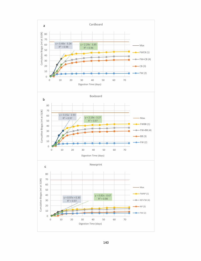
140
y = 0.97x + 0.30R² = 0.97
y = 0.82x - 0.67R² = 0.98
0
10
20
30
40
50
60
70
80
0 10 20 30 40 50 60 70
Cum
ulat
ive
Biog
as (m
l at 3
10K)
Digestion Time (days)
Newsprint
Max.
FWNP (1)
NP+FW (4)
NP (3)
FW (2)
c
y = 3.15x - 2.93R² = 0.97 y = 2.19x - 3.27
R² = 0.97
0
10
20
30
40
50
60
70
80
0 10 20 30 40 50 60 70
Cum
ualti
ve B
ioga
s (m
l at 3
10K)
Digestion Time (days)
Boxboard
Max.
FWBB (1)
FW+BB (4)
BB (3)
FW (2)
y = 3.40x - 3.26R² = 0.98
y = 2.29x - 3.85R² = 0.96
0
10
20
30
40
50
60
70
80
0 10 20 30 40 50 60 70
Cum
ulat
ive
Biog
as (m
l at 3
10K)
Digestion Time (days)
Cardboard
Max
FWCB (1)
FW+CB (4)
CB (3)
FW (2)
a
b

141
In an experiment designed to compare the digestibility of the fibre mixture at different levels of food
waste addition (Figure 9.7), it was found that the increase in digestion rate is very high at the beginning
of the experiment (>110%), then rapidly falls as digestion proceeds, finally levelling off at about 30% at
around 30 days. The extent of this effect seems to be completely independent of the amount of food
waste added, contradicting the coupon data obtained from Daisy, which showed that the greater the
amount of food waste added, the greater the digestibility of the substrates (with the exception of
newsprint and bulking agent). It seems highly likely that the optimum conditions of a BMP, namely
ample inoculum, macro and micro nutrients, and the fine particle size distribution of the substrate play
a role in this discrepancy.
y = 6.93x - 5.93R² = 1.00
y = 6.02x - 8.65R² = 0.91
0
10
20
30
40
50
60
70
80
0 10 20 30 40 50 60 70
Cum
ulat
ive
Biog
as (m
l at 3
10K)
Digestion Time (days)
Fine Paper
Max.
FPFW (1)
FP+FW (4)
FP (3)
FW (2)
y = 1.01x - 0.36R² = 1.00
y = 0.88x - 0.10R² = 0.98
0
10
20
30
40
50
60
70
80
0 10 20 30 40 50 60 70
Cum
ulat
ive
Biog
as (m
l at 3
10K)
Digestion Time (days)
Bulking Agent
Max.
FWBA (1)
FW+BA (4)
BA (3)
FW (2)
Figure 9.5 Calculation of synergy – normalized for COD content a) CB; b) BB; c) NP; d) FP; e) BA. The difference in initial gradients represents the effect of FW on the rate of biogas production from each fibre
e
d

142
BMP 2 contributed a great deal to the understanding of the digestibility of the fibres and the
synergistic effect brought about by food waste addition, but it did not answer questions about the
underlying mechanism. There seem to
be four possibilities;
Changes in the diversity and
abundance of the microbial
community
Changes in C:N ratio
Loss of nutrients present in
FW
The presence of enzymes in
the FW (or as products of
digestion of the FW) which
directly assist the hydrolysis of
the FB or
Some combination of these.
The complementary research being carried out by Peter HyunWoo Lee should be able to address the
first. The second and third are possible, but the effect on biogas production of changes in FW addition -
58.1
36.3 35.124.7
12.9
60.0
38.4 36.731.6
14.3
1.3
7.25.6
0.8
0.5
2.6
9.0 7.5
2.0
2.7
0
10
20
30
40
50
60
70
Cum
ulat
ive
Biog
as m
L. (a
t 310
K) 39 days 74 days
Figure 9.6 Synergy by fibre at 39d and 74d; normalized to constant COD; synergistic contribution in dark shading
0
20
40
60
80
100
120
140
0 20 40 60 80
Perc
ent I
ncre
ase
in B
ioga
s Pro
duct
ion
from
Fib
re
Digestion Time (days)
Synergy vs. Digestion Time - Effect of FW addition
FW 6%CODFW 8%CODFW 11%CODFW 17%CODFW 20%CODFW 27%COD
Figure 9.7 Percent increase in biogas yield, as a result of FW addition vs time, at six levels of food waste addition

143
rapid when FW is reduced, slower when FW is increased - would suggest something more complex. A
single leach bed with less food cannot alter the nutrient concentration by more than 3 or 4%; likewise
the C:N ratio. When the FW content in Daisy’s feed was reduced, the effect on biogas production was
almost instantaneous, and within 2 to 4 weeks biogas production had stabilized at a lower level (Figure
8.11). The next reduction, and the next, produced exactly the same effect. When the CODFW was all
added back in Week 50, gas production jumped in the first week, grew more modestly over the next
five weeks, then produced two big jumps in Weeks 56 and 57 (Section 8.3.3, Fig. 8.12). This perhaps
suggests that some critical condition had been reached that promoted synergy; in all it took 8 weeks to
restore gas production to its former level (Figure 8.11). These observations would suggest that the
synergy is in some way caused by the FW, and that the magnitude of the effect is related to the CODFW
addition rate, but that once CODFW is added back, it takes time for gas production to fully return. In
contrast, when Daisy was restarted at Week 26 after a 10d shutdown, gas production immediately rose
to exceed the prior weekly rate by about 100 L.wk-1 (20%). This lasted for three weeks suggesting that
Daisy was converting intermediate products that had accumulated during the shutdown.
Yun (2015) showed that the addition of small amounts of FW enhanced the digestion of waste activated
sludge, and that extracellular hydrolytic protease was primarily responsible. Yuan (2012) showed that
pre-treatment of waste paper and cardboard with a microbial consortium enhanced methane
production, and used the same method to quantify synergy as the one used in this work. The
consortium was specifically developed to degrade cellulose under thermophilic conditions, but has not
been fully characterized. This work offers some insight into possible causes, and more study will be
required, but there is evidence in the literature that enzymatic activity is the mechanism by which
biogas yields from paper and cardboard are enhanced. This is explored further in Section 9.2.
9.1.2 Biochemical Methane Potential Test 3 – One Litre Bottles and Coarse Substrate
Although BMP 2 provided great insight into the digestibility of individual substrates, and the effect of
food waste addition on biogas yield and rate, it was conducted under idealized conditions of finally-
divided substrates, excess inoculum and an anaerobic medium complete with all necessary macro and
micro nutrients, and the entire system was appropriately buffered. This approach falls short of
mimicking the behaviour in Daisy in four specific ways; substrate preparation, quantity of inoculum,
lack of leachate recirculation, inability to add food waste progressively to sealed bottles.
BMP 3 was designed to obviate three of these four differences (introducing leachate recirculation was obviously not possible);

144
Add substrates in exactly the same form as they were fed to Daisy (necessitating the use of 1 L bottles).
Add 120 g of substrate COD per bottle, 1/20 of the quantity of COD fed to one of Daisy’s leach beds.
Use leachate and sludge recovered at the conclusion of Period 6 from Tank 2 of Daisy as inoculum.
Equip three of the bottles with a gas-tight food waste feeding port. On paper, this concept was fine but it did create a
practical problem; measuring the volume of biogas
produced on this scale would be a challenge. A 160
mL serum bottle could be expected to produce 60
mL of biogas over a 10 week period. Under the
proposed plan each bottle would generate
approximately 60,000 mL of biogas over the
duration of the experiment. Professor Savia
Gavazza offered her knowledge and expertise to
solve this and other related challenges.
Experimental Setup Figure 9.8 is a schematic of Savia’s experimental
setup. As biogas is produced in Bottle a) it leaves
under slight pressure through plastic tubing and a
hypodermic needle into Bottle b) where it passes
through a solution of sodium hydroxide that scrubs
out the CO2; it also contains bromothymol blue
which turns green at pH 7.6. As gas accumulates in
b CH4
Biogas
Substrate
Water bath 37°C
NaOH in
Displacement gas meter and CO2 scrubber
NaOH soln.
Vent
Figure 9.8 Large BMP experimental set-up
c a
Plate 15. BMP 3; Substrate bottles a) in water bath (rear); gas meter bottles b) above and c) bottom foreground
Plate 16 BMP 3 Entire set-up with 11 bottles

145
Bottle b) it displaces the scrubbing medium to Bottle c). Periodically, as required, Bottle c) is removed
and weighed and the contents returned to Bottle b). This last step requires clamping the gas line and
physically removing and replacing Bottle b). Occasionally, scrubbing solution accumulates in the line
between Bottle b) and Bottle c); the clamped side arm is used to correct this condition. Plate 15 shows
a close-up of how the bottles are assembled; Plate 16 shows the complete set-up, with the water bath
in a spill containment tray, and the entire experiment housed within a fume hood. Though Savia and I
planned the experiment, built the system, and started it up together, the design concept and all the
subsequent gas measurement and analytical work were performed by Savia.
The experiment was set up as follows;
Experiments 1, 2 and 3 all contained cardboard (CB), boxboard (BB), newsprint (NP) and fine
paper (FP) in the same proportions as were fed to Daisy and in the same physical form; the
total mass added was 55 g (cf Daisy at 1,100 g). To ensure uniformity, each fibre was weighed
separately for each bottle.
Experiments 1 and 2 had food waste (FW) added at CODFW28%; Experiment 3 contained fibre
alone.
Experiment 1 was equipped with a gas-tight port to allow periodic injection of additional FW.
Two controls were run; one bottle containing glucose plus inoculum and one bottle containing
inoculum alone.
Table 9.5 Total Quantities of Substrates, Inoculum and Medium for BMP3, Large BMP (g unless otherwise stated)
Expt. No. CB BB NP FP FB FW (pulp)
FW/wk FWTotal Inoc LT (mL) Glucose
1 a,b,c FB+FW+FWadded 22.0 17.5 5.5 10.0 55.0 156.0 4.5 192.0 600
2 a,b,c FB+FW 22.0 17.5 5.5 10.0 55.0 156.0 156.0 600
3 a,b,c FB 22.0 17.5 5.5 10.0 55.0 600
4a NCON 600
4b PCON 46 554 2.0
CODsubstrate = 83.62 g/bot. (1 and 2) 62.17 g/bot. (3) VSinoculum = 15.5 g.L-1 9.3 g VS per bottle CODsubstrate:VSinoculum ratio = 9.0:1 lower than previous BMPs, lower than lit. recommends, but replicates Daisy CODglucose:VSinoculumratio= 3.0:1 0.71 gTS inoculum per bottle 45.8 mL LT+ sludge
Expt No. Description COD Content long-term averages (dry method)
1 a,b,c FB blend + FW at 28% by COD + 4.5g FWadded/wk Subs. CB BB NP FP FW Glucose
2 a,b,c FB blend + FW at 55 wt% (28% by COD) CODg/g 1.14 1.13 1.33 1.00 1.30 1.07
3 a,b,c FB blend 4a Negative control, Inoculum alone
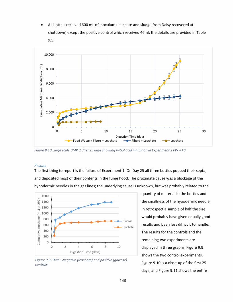
146
All bottles received 600 mL of inoculum (leachate and sludge from Daisy recovered at
shutdown) except the positive control which received 46ml; the details are provided in Table
9.5.
Results The first thing to report is the failure of Experiment 1. On Day 25 all three bottles popped their septa,
and deposited most of their contents in the fume hood. The proximate cause was a blockage of the
hypodermic needles in the gas lines; the underlying cause is unknown, but was probably related to the
quantity of material in the bottles and
the smallness of the hypodermic needle.
In retrospect a sample of half the size
would probably have given equally good
results and been less difficult to handle.
The results for the controls and the
remaining two experiments are
displayed in three graphs. Figure 9.9
shows the two control experiments.
Figure 9.10 is a close-up of the first 25
days, and Figure 9.11 shows the entire
Figure 9.10 Large scale BMP 3; first 25 days showing initial acid inhibition in Experiment 2 FW + FB
0
2,000
4,000
6,000
8,000
10,000
0 5 10 15 20 25 30
Cum
ulat
ive
Met
hane
Pro
duct
ion
(mL)
Digestion Time (days)Food Waste + Fibers + Leachate Fibers + Leachate Leachate
0
200
400
600
800
1000
1200
1400
1600
0 2 4 6 8 10
Cum
ulat
ive
met
hane
(mL)
at 2
97K
Digestion Time (days)
Glucose
Leachate
Figure 9.9 BMP 3 Negative (leachate) and positive (glucose) controls

147
experiment as cumulative methane production versus time. The positive control converted 96% of the
glucose added. The negative control generated 737 mL of methane (at 297K) by day eight. The negative
control is also shown in Figures 9.10 and 9.11; it has not been subtracted from the totals. The
differences between Experiment 2 (fibre + food waste) and Experiment 3 (fibre alone) are striking.
During the first three days, Experiment 2 produced a short-lived burst of methane then slowed to a
crawl for the next 10 days. It appears likely that the bottles became acidic as a result of the rapid
hydrolysis of food waste, and until that acid was consumed digestion was partially inhibited. This is
supported by the finding that at Day 17, shortly before it failed, Experiment 1 had dropped to pH 5.2,
an inhibitory condition presumably brought about by the FW it contained. During the same period,
methane production in Experiment 3 (fibre alone) began more slowly, caught up with Experiment 2 by
Day 10, then overtook it. The curves crossed again at day 17, at which point methane production in
Experiment 2 rose sharply for about 50 days before beginning to slow, after which the two cumulative
gas curves ran more or less parallel again. Experiment 3 produced methane at a very steady rate
throughout, finally ending at 11,378 mL of methane and 49% COD conversion, while Experiment 2
ended at 24,315 mL of methane and 81% COD conversion. Synergy was calculated as the percent
increase in methane production from fibre as a result of food waste addition, using the method
previously described. It was found to be 73% at 70 days, and 45% at 112 days. This decline in synergistic
contribution with time was also observed in the previous BMPs. Given enough time, fibre without food
0
2,000
4,000
6,000
8,000
10,000
12,000
14,000
16,000
18,000
20,000
22,000
24,000
26,000
0 5 10 15 20 25 30 35 40 45 50 55 60 65 70 75 80 85 90 95 100 105 110 115
Cum
ulat
ive
Met
hane
Pro
duct
ion
(mL)
Experimental Time (days)
49% COD conversion
737 mL of CH4 from leachate, 8167 mL CH4 from FW at 297K
81% COD conversion
Leachate
Experiment 3 FB
Experiment 2 FB + FWSynergy at 71d = 73%
Synergy at 112d = 45%
Figure 9.11 Large-scale BMP to 112 days; acid inhibition reverses itself in Exp. 2, methane production rises sharply, synergy evident
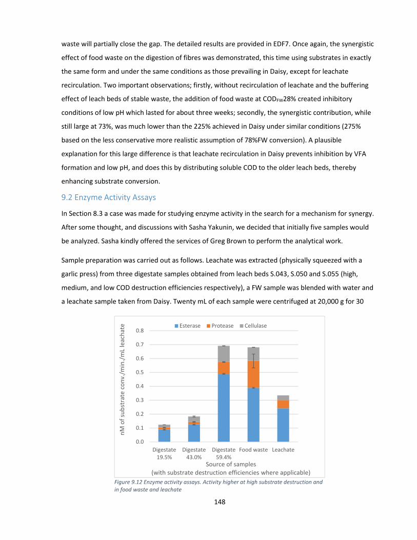
148
waste will partially close the gap. The detailed results are provided in EDF7. Once again, the synergistic
effect of food waste on the digestion of fibres was demonstrated, this time using substrates in exactly
the same form and under the same conditions as those prevailing in Daisy, except for leachate
recirculation. Two important observations; firstly, without recirculation of leachate and the buffering
effect of leach beds of stable waste, the addition of food waste at CODFW28% created inhibitory
conditions of low pH which lasted for about three weeks; secondly, the synergistic contribution, while
still large at 73%, was much lower than the 225% achieved in Daisy under similar conditions (275%
based on the less conservative more realistic assumption of 78%FW conversion). A plausible
explanation for this large difference is that leachate recirculation in Daisy prevents inhibition by VFA
formation and low pH, and does this by distributing soluble COD to the older leach beds, thereby
enhancing substrate conversion.
9.2 Enzyme Activity Assays
In Section 8.3 a case was made for studying enzyme activity in the search for a mechanism for synergy.
After some thought, and discussions with Sasha Yakunin, we decided that initially five samples would
be analyzed. Sasha kindly offered the services of Greg Brown to perform the analytical work.
Sample preparation was carried out as follows. Leachate was extracted (physically squeezed with a
garlic press) from three digestate samples obtained from leach beds S.043, S.050 and S.055 (high,
medium, and low COD destruction efficiencies respectively), a FW sample was blended with water and
a leachate sample taken from Daisy. Twenty mL of each sample were centrifuged at 20,000 g for 30
0.0
0.1
0.2
0.3
0.4
0.5
0.6
0.7
0.8
Digestate19.5%
Digestate43.0%
Digestate59.4%
Food waste Leachate
nM o
f sub
stra
te c
onv.
/min
./m
L le
acha
te
Source of samples (with substrate destruction efficiencies where applicable)
Esterase Protease Cellulase
Figure 9.12 Enzyme activity assays. Activity higher at high substrate destruction and in food waste and leachate

149
minutes; two of the samples did not pellet well, and were centrifuged again at 24,000 g; the
supernatant was recovered with a pipette. Each sample was spin-filtered at 3,600 g to concentrate the
proteins. Greg performed the following analyzes on each sample; total protein (Bradford Assay), and
enzyme activity for esterase, protease and cellulase; the procedures, including standard substrates, can
be found in Appendix C. Protein separation by denaturing gradient gel electrophoresis was also carried
out, and samples of the bands excised, and analyzed by Andy Quaile using a gas chromatograph/mass
spectrometer (GCMS) in an unsuccessful attempt to identify specific enzymes. Ideally, a metagenome
for the microbial population was required to do this successfully. The results for all the samples are
presented in Table 9.6 and Figure 9.12. The measured esterase, protease, and cellulase activity,
expressed as µM of subst. conv./min./ml extract, correlates well with COD destruction efficiency; both
the leachate and FW showed enzymatic activity too. The activity, in all cases, appears related to the
amount of food waste added, and consequently the substrate digestion efficiency. The food waste itself
also exhibits a level of enzyme activity that at least implies that FW is a source of enzymes similar to
those present in the digestate. The inference from this analysis is that synergy, at least in part, is an
enzymatic phenomenon and dependent upon the amount of food waste added.
Table 9.6 Enzyme Activity Assays
Sample Total Protein in Gel Enzyme Activity Activity
Description COD Destr. Effic.
%
OD - corrected for spin filter conc. µM of subst.
conv./min/mg of protein
nM of subst. conv./min/ml extract
Vol. µl
Conc. µg/µl
Mass µg
Ester Prot Cell X Conc
Ester. Prot. Cell. Ester. Prot. Cell.
S.043 19.5 12.5 0.16 2.00 0.089 0.015 0.020 42 8.27 0.23 1.90 7.87 0.22 0.30
S.050 43.0 12.5 0.4 5.00 0.125 0.019 0.039 36 4.00 0.10 1.24 11.1 0.28 0.57
S.055 59.4 12.5 0.15 1.88 0.489 0.086 0.116 7.4 8.58 0.25 2.03 43.5 1.3 1.7
FW (S.073)
12.5 0.62 7.75 0.389 0.194 0.098 12.7 2.83 0.24 0.71 34.6 2.9 1.5
Leach. 19/08/16 12.5 0.03 0.38 0.241 0.059 0.034 11.6 33.19 1.36 4.69 21.5 0.9 0.5
9.3 Composting of Digestate
The digestate produced by Daisy is still biologically active, but it is not stable, it is not sterilized and
must be aerobically cured (composted). The initial plan was to cure the digestate by aerating it in the
leach beds at the conclusion of the digestion period, generally 42 days. As reported previously it was
not possible to do this on such a small scale. All the digestate was saved, stored at 4°C until the end of
the experiment, then transported to Miller Waste Systems for aerobic curing in a single batch
experiment of about 300 kg. The work was conducted by Kyle Schumacher of Miller, and it is his
summary, with my edits, which follows.
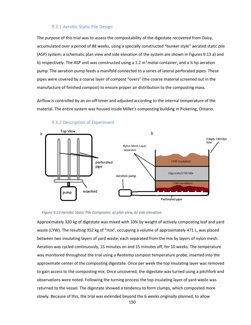
150
9.3.1 Aerobic Static Pile Design
The purpose of this trial was to assess the compostability of the digestate recovered from Daisy,
accumulated over a period of 88 weeks, using a specially constructed “bunker style” aerated static pile
(ASP) system; a schematic plan view and side elevation of the system are shown in Figures 9.13 a) and
b) respectively. The ASP unit was constructed using a 1.2 m3 metal container, and a ¼ hp aeration
pump. The aeration pump feeds a manifold connected to a series of lateral perforated pipes. These
pipes were covered by a coarse layer of compost “overs” (the coarse material screened out in the
manufacture of finished compost) to ensure proper air distribution to the composting mass.
Airflow is controlled by an on-off timer and adjusted according to the internal temperature of the
material. The entire system was housed inside Miller’s composting building in Pickering, Ontario.
9.3.2 Description of Experiment
Approximately 320 kg of digestate was mixed with 10% by weight of actively composting leaf and yard
waste (LYW). The resulting 352 kg of “mix”, occupying a volume of approximately 471 L, was placed
between two insulating layers of yard waste, each separated from the mix by layers of nylon mesh.
Aeration was cycled continuously, 15 minutes on and 15 minutes off, for 10 weeks. The temperature
was monitored throughout the trial using a Reotemp compost temperature probe, inserted into the
approximate center of the composting digestate. Once per week the top insulating layer was removed
to gain access to the composting mix. Once uncovered, the digestate was turned using a pitchfork and
observations were noted. Following the turning process the top insulating layer of yard waste was
returned to the vessel. The digestate showed a tendency to form clumps, which composted more
slowly. Because of this, the trial was extended beyond the 6 weeks originally planned, to allow
Figure 9.13 Aerobic Static Pile Composter; a) plan view, b) side elevation
a b

151
additional time and additional turning to improve the quality of the product. Samples of the leaf and
yard waste, digestate, starting mix, and resulting composted digestate were sent to A&L labs for
analysis and the results are presented below. Plate 17 shows the ASP in operation; what it lacks in
beauty it makes up for in performance.
9.3.3 Results
Upon receipt, the raw digestate had a mild “rotting/putrid” odour, which only lasted for about three
weeks. By week four the digestate had taken on a pleasant earthy odour. The digestate consisted
primarily of remnants of cardboard/paper materials from the anaerobic digestion process, and had a
moisture content of 75%. To help induce proper composting, 10% by weight of actively composting leaf
and yardwaste was added, reducing density and moisture content slightly. The most challenging
characteristic of the digestate for composting purposes was the clumping of the material. Some of
these clumps were already formed, some formed during the trial. Efforts were made to break them up
using a pitchfork during the turning process, to increase surface area for microbial activity;
nevertheless, some clumping remained. On a commercial scale these clumps would be broken up by
mechanical equipment (Scarab turners, loaders, etc.) and would not be an issue. The extension of the
compost trial to 10 weeks allowed most of the clumps to be broken up in a way that simulated a
commercial operation.The light beige/grey appearance of the mix changed quickly once the materials
Plate 17. Aerobic Static Pile Composter; housed inside compost building; note blower on the left and piping
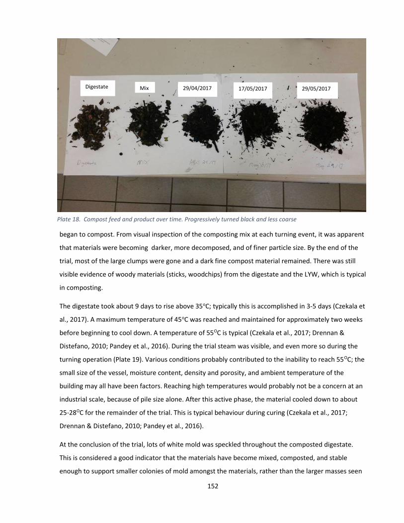
152
began to compost. From visual inspection of the composting mix at each turning event, it was apparent
that materials were becoming darker, more decomposed, and of finer particle size. By the end of the
trial, most of the large clumps were gone and a dark fine compost material remained. There was still
visible evidence of woody materials (sticks, woodchips) from the digestate and the LYW, which is typical
in composting.
The digestate took about 9 days to rise above 35oC; typically this is accomplished in 3-5 days (Czekala et
al., 2017). A maximum temperature of 45oC was reached and maintained for approximately two weeks
before beginning to cool down. A temperature of 55OC is typical (Czekala et al., 2017; Drennan &
Distefano, 2010; Pandey et al., 2016). During the trial steam was visible, and even more so during the
turning operation (Plate 19). Various conditions probably contributed to the inability to reach 55OC; the
small size of the vessel, moisture content, density and porosity, and ambient temperature of the
building may all have been factors. Reaching high temperatures would probably not be a concern at an
industrial scale, because of pile size alone. After this active phase, the material cooled down to about
25-28OC for the remainder of the trial. This is typical behaviour during curing (Czekala et al., 2017;
Drennan & Distefano, 2010; Pandey et al., 2016).
At the conclusion of the trial, lots of white mold was speckled throughout the composted digestate.
This is considered a good indicator that the materials have become mixed, composted, and stable
enough to support smaller colonies of mold amongst the materials, rather than the larger masses seen
Plate 18. Compost feed and product over time. Progressively turned black and less coarse
Digestate Mix 29/04/2017 17/05/2017 29/05/2017
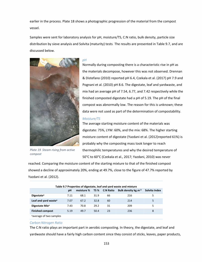
153
earlier in the process. Plate 18 shows a photographic progression of the material from the compost
vessel.
Samples were sent for laboratory analysis for pH, moisture/TS, C:N ratio, bulk density, particle size
distribution by sieve analysis and Solvita (maturity) tests. The results are presented in Table 9.7, and are
discussed below.
pH Normally during composting there is a characteristic rise in pH as
the materials decompose, however this was not observed. Drennan
& Distefano (2010) reported pH 6.4, Czekala et al. (2017) pH 7.9 and
Pognani et al. (2010) pH 8.6. The digestate, leaf and yardwaste, and
mix had an average pH of 7.54, 6.77, and 7.42 respectively while the
finished composted digestate had a pH of 5.19. The pH of the final
compost was abnormally low. The reason for this is unknown; these
data were not used as part of the determination of compostability.
Moisture/TS The average starting moisture content of the materials was
digestate: 75%, LYW: 60%, and the mix: 68%. The higher starting
moisture content of digestate (Yazdani et al. (2012)reported 61%) is
probably why the composting mass took longer to reach
thermophilic temperatures and why the desired temperature of
50°C to 60°C (Czekala et al., 2017; Yazdani, 2010) was never
reached. Comparing the moisture content of the starting mixture to that of the finished compost
showed a decline of approximately 20%, ending at 49.7%, close to the figure of 47.7% reported by
Yazdani et al. (2012).
Carbon:Nitrogen Ratio The C:N ratio plays an important part in aerobic composting. In theory, the digestate, and leaf and
yardwaste should have a fairly high carbon content since they consist of sticks, leaves, paper products,
Table 9.7 Properties of digestate, leaf and yard waste and mixture
pH moisture % TS % C:N Ratio Bulk density kg.m-3 Solvita Index
Digestatea 7.11 68.1 31.9 66 216 5
Leaf and yard wastea 7.07 67.2 32.8 60 214 5
Digestate Mixa 7.43 70.8 29.2 31 209 5
Finished compost 5.19 49.7 50.4 23 236 8 aaverage of two samples
Plate 19 Steam rising from active compost

154
and ash wood chips. However, the reported C:N ratios for the starting materials on the first set of
samples analyzed showed a large discrepancy and were obviously incorrect. Based on the more realistic
values from the second set of samples, the C:N ratio of the mix was 31:1, falling to 23:1 at the end of
the composting period; this is within the normal range as reported by Czekala et al. (2017).
Bulk density The bulk density on a dry weight basis increased from 201 kg.m-3 to 236 kg.m-3 for the finished compost;
these are typical values measured at full scale by Miller Waste Systems Inc.
Solvita (maturity) The most important method for determining compostability is the measurement of microbial activity
using the Solvita test, a commercially available test which combines measurements of the decline in
production of NH3and CO2 as composting progresses (Drennan & Distefano, 2010). The result is
compared to a Solvita index scale of 1 to 8; the higher the number the lower the CO2/NH3 emissions
and the better the product. A Solvita index of 7 or 8 is required in Ontario to demonstrate mature
finished compost.
The starting materials, including the digestate mix, all showed a Solvita index of 5. Though raw organic
waste typically has an index closer to 3, thisvalue was expected since the digestate had already been
anaerobically treated and the volatile carbon content reduced. During the trial, several samples were
collected and had their Solvita index measured to track progress. The index remained at 5 until about
Week 7 when the index fell to 6. At 10 weeks however the finished compost showed a fully mature
index of 8. Having gone from an index of 5 to 8 confirms the compostability of digestate, and confirms
its potential use as a finished compost material.
Sieve analysis Sieve analyses of the beginning mix and the finished compost were performed using screen sizes typical
for compost analysis. The two samples of digestate mix from the start of the experiment had quite
different particle size distributions, but the finished compost was certainly finer than the starting
materials. An increase from 26% to 43% of material passing the ¼” sieve was observed, giving further
confirmation of the compostability of
the digestate. The difference was easily
seen in a visual comparison of the two
materials.
Table 9.8 Sieve analysis of digestate mix and compost - percent minus
Sieve size 2" 1" 1/2" 3/8" 1/4"
Digestate Mixa 100.0 97.8 60.2 44.6 26.0
Finished compost 100.0 82.9 63.7 57.2 43.0 aaverage of two samples

155
9.3.4 Aerobic Curing Conclusions
The final compost had a desirable “earthy compost” odour. The physical evidence of composting was
very apparent; the colour changed from beige/gray to a very dark earthy colour with a considerable
proportion fine particles. There was still evidence of clumps that had not been broken up properly
during the trial. Smaller particle size was also measured by the final sieve analysis. The Solvita test, the
best indicator of compostability, resulted in an index of 8 (fully mature compost).
Unfortunately the C:N ratio and pH data could not be used with confidence to prove or disprove
compostability. However, with the remaining data, physical observations, and temperature behavior
observed, it can be concluded that the digestate is compostable.
The composting process could have been improved by increasing the active yard waste proportion to
20-25% to decrease composting time, and encourage higher temperatures. On a commercial scale,
results would also benefit from larger pile size, higher ratios of active compost to digestate, and the use
of mechanical turning to break up clumping.
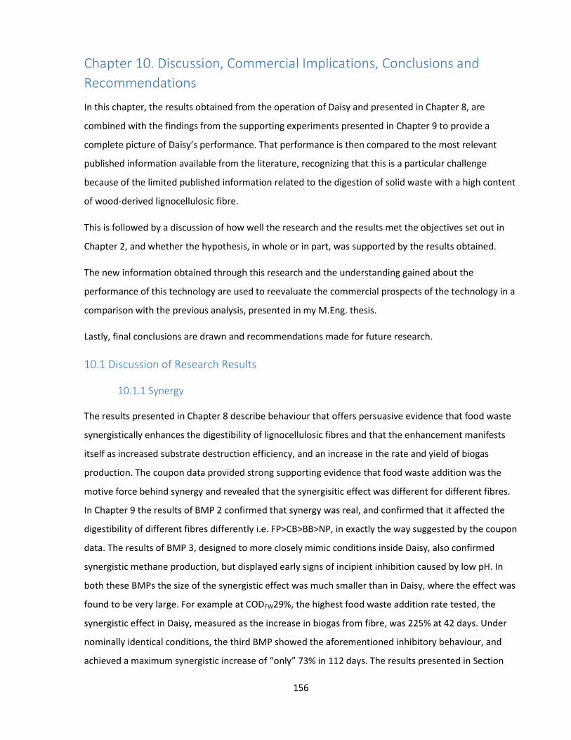
156
Chapter 10. Discussion, Commercial Implications, Conclusions and Recommendations
In this chapter, the results obtained from the operation of Daisy and presented in Chapter 8, are
combined with the findings from the supporting experiments presented in Chapter 9 to provide a
complete picture of Daisy’s performance. That performance is then compared to the most relevant
published information available from the literature, recognizing that this is a particular challenge
because of the limited published information related to the digestion of solid waste with a high content
of wood-derived lignocellulosic fibre.
This is followed by a discussion of how well the research and the results met the objectives set out in
Chapter 2, and whether the hypothesis, in whole or in part, was supported by the results obtained.
The new information obtained through this research and the understanding gained about the
performance of this technology are used to reevaluate the commercial prospects of the technology in a
comparison with the previous analysis, presented in my M.Eng. thesis.
Lastly, final conclusions are drawn and recommendations made for future research.
10.1 Discussion of Research Results
10.1.1 Synergy
The results presented in Chapter 8 describe behaviour that offers persuasive evidence that food waste
synergistically enhances the digestibility of lignocellulosic fibres and that the enhancement manifests
itself as increased substrate destruction efficiency, and an increase in the rate and yield of biogas
production. The coupon data provided strong supporting evidence that food waste addition was the
motive force behind synergy and revealed that the synergisitic effect was different for different fibres.
In Chapter 9 the results of BMP 2 confirmed that synergy was real, and confirmed that it affected the
digestibility of different fibres differently i.e. FP>CB>BB>NP, in exactly the way suggested by the coupon
data. The results of BMP 3, designed to more closely mimic conditions inside Daisy, also confirmed
synergistic methane production, but displayed early signs of incipient inhibition caused by low pH. In
both these BMPs the size of the synergistic effect was much smaller than in Daisy, where the effect was
found to be very large. For example at CODFW29%, the highest food waste addition rate tested, the
synergistic effect in Daisy, measured as the increase in biogas from fibre, was 225% at 42 days. Under
nominally identical conditions, the third BMP showed the aforementioned inhibitory behaviour, and
achieved a maximum synergistic increase of “only” 73% in 112 days. The results presented in Section

157
8.4, describing biogas production from an individual leach bed, and rising leach bed temperatures after
fresh waste was added, suggest that the buffering effect of partly digested substrates, combined with
leachate recirculation, enhanced the synergistic effect in Daisy, compared to the static conditions of the
BMP. If this is true, the sequentially-fed leach beds, central to the design of Daisy, play an important
role in synergy as well as enhancing stability, and overall performance.
A plausible mechanism for synergy was needed, together with some additional confirmatory evidence.
A mechanism involving the presence or absence of specific methanogens was discussed in Section 8.3.5
and shown to be inconsistent with VFA creation and consumption. Another possibility, that synergy is
an enzymatic process whereby hydrolytic enzymes already present in the FW or created as a product of
FW digestion, seems more plausible.
The enzyme activity assay provided evidence that enzymatic activity is at least partly responsible for
synergy. Gan et al. (2003), in a review paper on the enzymatic hydrolysis of cellulose, determined that
this is a surface phenomenon, and that only a small fraction of the cellulosic substrate is undergoing
active hydrolysis at any given moment (less than 2% for particles smaller than 100 µm). Zhang et al.
(2007) conducted experiments on the digestion of vegetable and flower wastes in a two-stage digester
comprising a single leach bed and a methanogenic reactor. Leachate was recirculated through the leach
bed but was diluted with the effluent from the methanogenic reactor. They were able to show that this
experimental arrangement accelerated the degradation of the solid wastes, and that hydrolysis was
enhanced by the dilution effect of the methanogenic reactor effluent. They also found that the
hydrolysis of these organic solid wastes was mainly attributable to cell-free enzymes, followed by
biofilm-associated enzymes; the relative contribution of each remaining a matter of debate. Pommier
et al. (2010) in an experiment digesting samples of paper and cardboard, under conditions in which
enzyme concentration was not a limiting factor, concluded that substrate size reduction did not
improve accessibility to enzyme binding sites. Judging from the pseudo-zero order graphs of biogas
production for individual fibres in BMP 2 (Section 9.1.1), hydrolysis was being governed by substrate
availability in the form of the surface phenomenon described by Gan et al. (2003). If this is correct, and
the synergistic effect is attributable to enzymes present in food waste, or created by its digestion,
hydrolysis in Daisy must still be enzyme-limited, because the synergistic effect had not levelled off even
at the highest CODFW addition (Figure 8.16). In summary there is persuasive evidence, in both literature
and in the results of this study, that synergy is the result of enzymatic activity and that this process is
enhanced by the leachate recirculation in a two-stage anaerobic digester and particularly the return of
UASB effluent to the leach beds.

158
One last word on synergy. All of the previous calculations of the magnitude of the synergistic effect
have been based on the assumption that 100% of CODFWadded is converted; but we know from BMP 2,
carried out under presumably ideal
conditions of inoculum/substrate ratio,
macro and micro nutrients, and very fine
particle size, that CODFW is only 78%
converted. If this conversion were translated
to Daisy’s results, what would this mean to
the magnitude of the synergistic effect?
Figure 10.1 reproduces Figure 8.16 (FW at
100% conversion) with FW at 78%
conversion added. The amount of synergistic
biogas produced is of course larger (by
26.6% at CODFW29.3%) and the relationship
between food waste added and synergistic biogas produced per kilogram of CODFB is linear, with a very
good regression coefficient. At some level of food waste addition this relationship must end. Perhaps
this will occur when the only
undigested portion of the fibres
remaining consists of lignin.
Plate 20 illustrates why 22% of
CODFW remains undigested. A
piece of corn cob from Daisy’s
digestate has been picked clean
of more easily digested
material, leaving a
lignocellulosic ‘skeleton’
behind, apparently resistant to
the effects of synergy. It is also possible to calculate the destruction efficiency of the fibres, on a COD
basis, from the synergy data. This is shown, calculated two ways, assuming 100%FW conversion and the
more realistic 78%FW conversion in Figure 10.2. Destruction efficiency is 63.6% at 29%CODFW vs. 16.5%
at 0%CODFW, a 285% increase (assuming 78% FW conversion).
y = 10.17xR² = 0.99
y = 8.04x + 4.03R² = 0.99
0
50
100
150
200
250
300
350
0 5 10 15 20 25 30 35
Syne
rgist
ic B
ioga
s L/k
gCO
Dfib
re a
dded
(at S
TP)
Percent CODtotal as FW
FW at 78% conv. FW at 100% conv.
n = 4
n = 4
n = 4
n = 16
n = 6
n = 6
For all x axis values n = 27
Figure 10.1 Synergistic biogas - FW at 78% conv. vs FW at 100% conv.
3 cm
Plate 20. Partially digested corn cob; unconvertible COD
159
Like the biogas yield curve, this suggests that still higher FB destruction efficiencies might be possible at
higher FW addition.
10.1.2 Aerobic Curing
The digestate from the digestion of solid waste must be composted to ensure that it is no longer
biologically active, and to turn it into a potentially usable product. This was the last unit operation
which needed to be demonstrated and was always considered to be essential to overall success; lab
scale tests on a small scale during Daisy’s operation failed, but a single experiment with all of Daisy’s
digestate was successful. The digestate is not difficult to compost and can be combined with other
wastes, such as leaf and yard waste, and co-composted without difficulty.
10.1.3 Comparison of Daisy’s Performance to the Literature Daisy’s performance is compared to the somewhat limited published information on the digestion of
similar substrates. The comparisons, shown in Table 10.1, are based on methane yield expressed as
mLCH4.g-1VSadded and destruction efficiency expressed as a % VSdestroyed. At CODFW29.3% Daisy’s yield was
296 mLCH4.g-1VSadded at a substrate destruction efficiency of 69.4% (as VS). Daisy’s results are shown at
six different levels of food waste addition and compared to those of four published studies; Pommier et
al. (2010), Yuan et al. (2012), Eleazer et al. (1997), and Zhang et al. (2012a). The first three specifically
studied wood-derived lignocellulosic fibres such as CB, BB, NP, and FP. Zhang et al.’s substrate was mr-
OFMSW but also included are their results for source separated food waste (ss- FW). For each, the type
Figure 10.2 Fibre destruction efficiency. Shows synergistic effect of FW addition
0
10
20
30
40
50
60
70
0 5 10 15 20 25 30
Perc
ent C
OD
fibre
Des
truc
tion
Percent CODtotal as Food Waste
100% FW conv. 78% FW Conv.
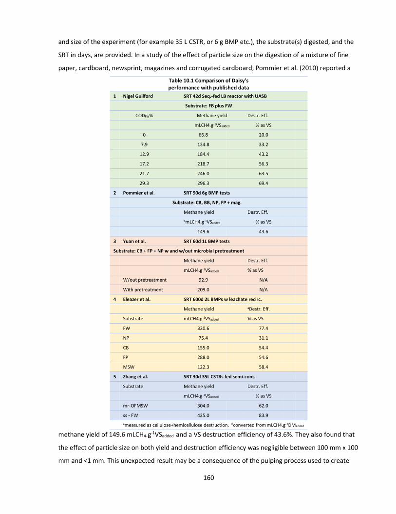
160
and size of the experiment (for example 35 L CSTR, or 6 g BMP etc.), the substrate(s) digested, and the
SRT in days, are provided. In a study of the effect of particle size on the digestion of a mixture of fine
paper, cardboard, newsprint, magazines and corrugated cardboard, Pommier et al. (2010) reported a
Table 10.1 Comparison of Daisy's performance with published data
1 Nigel Guilford SRT 42d Seq.-fed LB reactor with UASB
Substrate: FB plus FW
CODFW% Methane yield Destr. Eff. mLCH4.g-1VSadded % as VS
0 66.8 20.0
7.9 134.8 33.2
12.9 184.4 43.2
17.2 218.7 56.3
21.7 246.0 63.5
29.3 296.3 69.4
2 Pommier et al. SRT 90d 6g BMP tests
Substrate: CB, BB, NP, FP + mag.
Methane yield Destr. Eff.
bmLCH4.g-1VSadded % as VS
149.6 43.6
3 Yuan et al. SRT 60d 1L BMP tests
Substrate: CB + FP + NP w and w/out microbial pretreatment
Methane yield Destr. Eff.
mLCH4.g-1VSadded % as VS
W/out pretreatment 92.9 N/A
With pretreatment 209.0 N/A
4 Eleazer et al. SRT 600d 2L BMPs w leachate recirc.
Methane yield aDestr. Eff.
Substrate mLCH4.g-1VSadded % as VS
FW 320.6 77.4
NP 75.4 31.1
CB 155.0 54.4
FP 288.0 54.6
MSW 122.3 58.4
5 Zhang et al. SRT 30d 35L CSTRs fed semi-cont.
Substrate Methane yield Destr. Eff.
mLCH4.g-1VSadded % as VS
mr-OFMSW 304.0 62.0
ss - FW 425.0 83.9
ameasured as cellulose+hemicellulose destruction. bconverted from mLCH4.g-1DMadded
methane yield of 149.6 mLCH4.g-1VSadded and a VS destruction efficiency of 43.6%. They also found that
the effect of particle size on both yield and destruction efficiency was negligible between 100 mm x 100
mm and <1 mm. This unexpected result may be a consequence of the pulping process used to create

161
these products all of which, to varying degrees, are permeable. They also reported an inverse linear
relationship between lignin content and biodegradability – FP>CB>NP. The work of Yuan et al.(2012)
compared the digestion of mixed fibres (CB, FP and NP) with and without microbial pretreatment. The
purpose of the pretreatment was to enhance digestibility; a 125% increase in methane yield from 92.9
to 209.0 mLCH4.g-1VSadded was reported. Eleazer et al. (1997), in a simulation of anaerobic digestion in a
landfill of individual fibres (hence the 600 d SRT) obtained results similar to those of BMP 2 presented
in this thesis, except in the case of FP which appears to show a destruction efficiency which is too low
for the amount of methane produced. Daisy’s performance matched or surpassed that of all the
comparable work cited, except for Eleazer et al.’s (1997) result for food waste alone. In broad terms,
Daisy’s performance, processing coarser material, matched that of Zhang et al.’s (2012a) CSTR using
only 25% of the volumetric reactor capacity. Although Daisy’s SRT was 42 days, Figure 8.14 shows that
97.6% of ultimate substrate destruction had been achieved within 28 days.
In contrast, Zhang et al’s (2012a) results for ss-FW (source separated food waste) measured shortly
before reactor failure, show a methane yield of 425 mLCH4.g-1VSadded and destruction efficiency of
83.9% (compared to 304 mLCH4.g-1VSadded and 62% destruction efficiency for mr-OFMSW). This is partly
because FW is more digestible, but partly because it has a higher COD content per gVS than does
lignocellulosic fibres. Does this mean that Daisy could be operated with an SRT of 30 days instead of 42
days as suggested by Figure 8.14, the graph of substrate destruction versus time, and if so how could
this be accomplished? The data would suggest that SRT could be reduced but the supporting evidence
is limited (a single measurement obtained at CODFW29%). It also seems likely, based on Daisy’s
performance, that the curve shown in Figure 8.14 would look quite different at lower food waste
addition rates. Section 8.4 makes the argument that leach beds nearing the end of their digestion cycle
are still operating as methanogenic reactors and thereby contributing to process stability, thus
shortening the SRT could diminish or eliminate this benefit. Lastly, the possibility of eliminating the
UASB, also discussed in Section 8.4, must be factored in. A systematic study to address these
interconnected questions is proposed as part of the recommendations for future work in Section
10.3.2.
10.1.4 Properties of Bulking Agent
The addition of bulking agent to the waste provides structure and ensures continued drainage as the
waste digests. The physical characteristics of the bulking agent were not given much serious thought
until a decline in gas production and waste digestibility were observed during Period 5. At the time, it
appeared as though the manner in which the wood had been ground was at least partially responsible.
162
The experiments conducted to investigate this behaviour suggested that bulking agent properties were
the cause, but did not conclusively prove it; in the absence of any other explanation, I still believe it to
be true. Also, the amount of bulking agent used was based on the work of others (Murto et al., 2013)
and was not optimized for Daisy.
10.1.5 Meeting the Objectives
Five objectives were set out in Section 2.2:
1. Design, build, and commission a laboratory scale version of the Biopower process.
2. Test and troubleshoot the initial operation to confirm operability and create a baseline
for subsequent experiments.
3. Develop analytical methodology and a sampling plan compatible with the operation of
the digester that will enable mass and energy balance calculations and performance
monitoring and benchmarking to other systems.
4. Operate the reactor under a variety of test conditions to measure efficiency in terms of
biogas yield, COD destruction and solids stabilization, as well as robustness and
stability, starting with examining the effects of changes in substrate composition.
5. Use the performance data obtained to refine economic predictions for a full scale
system.
All of these objectives were met.
10.1.6 Testing the Hypothesis
The hypothesis comprises three sentences and is tested against the findings of this research
programme sentence by sentence. I have split the hypothesis accordingly and restated it below for
convenience:
1. An anaerobic digester, comprising multiple sequentially-fed leach beds feeding a single UASB is
capable of successfully processing mixed organic wastes, consisting of varying proportions of
cellulosic wastes (paper, cardboard, boxboard) and food waste, to produce commercial
quantities of biogas and a stabilized digestate.
Daisy was designed and built to conform to the concept of the patented BioPower process, with six
sequentially-fed leach beds and a single UASB. The capability of this design for processing a mixture of
cellulosic wastes and food waste was clearly demonstrated. The quantity of food waste added,
measured as a percentage of total COD, varied from 0 to 29%. At a solids retention time of 42 days
(which was maintained throughout the experiment with one minor exception), substrate digestibility
163
and biogas production varied considerably as a result of changes in food waste addition. It is doubtful
that commercial quantities of biogas could be generated under these conditions without the synergistic
effect contributed by the food waste. The upper limit of food waste addition, evidenced by the onset
of digester instability, was never reached. Given that food waste addition is shown to be so beneficial
to performance, and thus to the commercial prospects of the technology, the upper boundary of this
component of the hypothesis should be determined. Daisy’s performance matched that of a CSTR
digesting a similar substrate, and did so in a similar solids retention time. Section 10.3 compares
economic performance in 2009 with 2017. Despite a number of significant changes since 2009 (e.g.
cancellation of Ontario’s feed-in-tariff programme for electricity which was worth 14.7ȼ/kWh), the
financial returns (assisted by carbon credits at $5/GJ and robust tipping fees of $100/t) remain very
strong – a ten-year IRR of 41% and a year-10 EBIT of 54%. As was the case in 2009, an annual capacity
of 50 – 60,000 tonnes/y of organic waste is needed to achieve these results, and financial performance
is quite sensitive to capacity (Guilford, 2009).
2. This can be accomplished by managing the leach beds independently of one another, balancing
leachate flow between recirculation to the leach beds and delivery to the UASB, allowing
adequate solids retention time to achieve the maximum practical conversion of biomass to
biogas, and by aerobically curing the digestate.
The leach beds were managed independently of one another, the flow was balanced between
recirculation and delivery to the UASB and this worked successfully, but it would not be accurate to say
that this relationship was optimized. Varying flow to the leach beds requires that their temperature be
thermostatically controlled and, although leach bed heaters were installed in September 2015 with a
resultant increased biogas production, their control was manual. The necessity for a UASB was also not
demonstrated. On the one hand the UASB converts a lot of soluble COD immediately after fresh waste
(especially FW) is added, but on the other hand, when it was partially plugged and malfunctioning from
Week 55 to Week 60, there were no obvious ill-effects on overall performance. On the basis of the
single test near the end of the experimental programme (Figure 8.14) the solids retention time was
shown to be more than adequate at high levels of food waste addition. The aerobic curing step worked
well.
3. Digestion rate and yield can be enhanced by managing the proportion of food waste to fibres;
the production of waste water (except for water-of-saturation in the digestate) can be
minimized or even eliminated; process stability can be maintained, despite feedstock variability,
by controlling two principal variables; C:N ratio and alkalinity.

164
The discovery of synergy, and determination of its magnitude, demonstrated beyond all reasonable
doubt that adding food waste enhanced the digestion of fibres, and did so without upsetting Daisy’s
stability. The complete absence of wastewater (other than as water of saturation in the digestate) was
a pleasant surprise; managing effluent from anaerobic digesters is often a significant expense. All the
water of saturation in the digestate can be expected to evaporate in the aerobic curing step. Near the
end of the experiment, water addition to the feedstock was reduced in order to prevent leachate levels
rising too high in the tanks. From start to finish Daisy remained stable, the C:N ratio was always above
40 and the pH and alkalinity well within acceptable ranges, though it cannot be said that either one had
to be actively controlled in order to maintain stability. In fact, Daisy’s six leach beds meant that no more
than 16% of the waste could be changed at any one time, so it is hard to create conditions of instability
in the entire system: the design is inherently well-buffered and stable. There were signs towards the
end of the experiment that the concentration of inorganic salts within Daisy, particularly sulphate, was
starting to rise. This was attributable to increasing food waste addition and could ultimately require
that food waste addition be reduced. In summary, with some caveats, the hypothesis was found to be
well-supported.
10.2 Commercial Implications
In 2009 my M.Eng. thesis included a detailed financial analysis of the commercial prospects of the
BioPower technology. Much has changed since then; some of the changes have been favourable but
others not. In 2009 the model was based upon a generic design for a 60,000 tonne per year plant. In
2017, the model is based upon a specific project to be built in Ottawa with construction starting in
about two years, and is thus fundamentally different in certain respects. Table 10.2 summarizes the
major assumptions then and now. Plant capacity has been reduced by 10,000 tonnes per year but the
tipping fee has increased to $100 per tonne; this is the currently-prevailing market rate in the Ottawa
area. The amount of biogas recovered per tonne of
incoming waste has increased, and the SRTanaerobic has
been shortened to one year from three years and the
SRTaerobic from 18 months to nine months, all as a
direct consequence of Daisy’s results. These SRTs
differ markedly from those used in Daisy and this
requires some explanation. Compared to Daisy, a
commercial plant will be disadvantaged in three ways; firstly, the feedstock, as placed in the digester,
will be more heterogeneous and the distribution of leachate, and its penetration into the waste mass
Table 10.2 Financial Model - Major Assumptions
2009 2017
Plant capacity 60,000 50,000 tonnes/year
Tipping fee 70 100 $/tonne
Biogas recovered 150 250 m3/tonne
Power purchase 14.7 0 ¢/kWh
Natural gas sales 0 8 a$/tonne
Residue (10% incoming t) 70 60 $/tonne
Carbon credits 0 5 $/GJ

165
more uneven and slower as a result. Secondly, the digesting waste mass will partially collapse under its
own weight potentially affecting digestion efficiency. Thirdly, the regulators will insist that the waste be
stabilized and, as far as possible odour-
free, before it is exhumed. With time and experience,
shorter SRTs are probably achievable, so the design
must be conservative and yet accommodate this
possibility. The SRTs chosen come directly from the work
of Yazdani (2012) on a landfill-based anaerobic/aerobic
digester processing yard waste only and are thus very
conservative. Revenue from the sale of power has been eliminated because of the cancellation of
Ontario’s feed-in tariff (FIT) programme for renewable electricity from biogas (14.7ȼ/kWh). Carbon
credits have been added at $5/GJ.
The capital cost estimate in Table 10.3 shows an increase of about 11% but this is less of an effect of
inflation and more a reflection of changes in scope. The land purchase is a pro rata allocation of the
total cost of the lands acquired for the entire Ottawa project. The environmental approvals cost is
shown as zero because the total is not known, and its allocation to the various components of the
entire project has not been made. Costs have been reallocated between the treatment unit and site
preparation; this is largely an accounting exercise. The electrical plant has of course been eliminated.
Table 10.4 compares projected financial performance in 2009 and
2017. The underlying assumptions and a summary income
statement can be found in my M.Eng. thesis for 2009 (Guilford,
2009), and in Appendix G for 2017. The major differences are as
follows. The tipping fee revenues have increased, the net effect of
lower tonnages at a higher price per tonne. Energy sales are
much lower because of the cancellation of Ontario’s feed-in-tariff
programme which was worth 14.7ȼ/kWh . An allowance for
carbon credits has been added at $5/GJ. The compost revenue
has also been eliminated; the value of the compost is very
dependent upon the cleanliness of the incoming waste; this is less
certain for commercial waste. The EBITDA and EBIT numbers
given are for year 10, and the NPV and IRR are both calculated
over 10 years. Despite all the changes, the financial performance is still very strong. Apart from the
inevitable uncertainties associated with scale up, the financial performance depends most heavily on
Table 10.3 Capital Cost Summary
2009 2017
Land purchase $430,000 $1,670,000
Environmental Approvals $250,000 $0
Site preparation $3,243,000 $121,000
Treatment Unit $1,881,000 $7,741,000
Equipment $4,075,000 $5,386,000
Electrical plant $3,500,000 $0
Total $13,379,000 $14,915,000
Table 10.4 Year 10 Financial projections
2009 2017
Tipping fee 5,019,000 5,975,000
Energy sales 2,371,000 572,000
Carbon credits 0 1,430,000
Compost sale 752,000 0
Total Revenue 8,142,000 7,977,000
O&M costs 3,041,000 2,985,000
EBITDA 5,101,000 4,923,000
Deprec. 1,298,000 1,773,000
EBIT 3,803,000 3,220,000
NPV 6,053,000 6,534,000
IRR 43% 41%

166
tipping fees. However, if these were to drop to $50 per tonne the project would still be breakeven.
Under the terms of the environmental assessment approval granted for this project, the anaerobic
digestion facility will first be built at a demonstration scale of up to 20,000 tonnes per year.
10.3 Conclusions and Recommendations
10.3.1 Conclusions
Six principal conclusions can be drawn from the research. In order of significance, they relate to
synergy, digester performance, digester stability, reactor design, commercial prospects and greenhouse
gas emissions.
1. Synergy
The addition of food waste enhances the digestion of a mixture of lignocellulosic fibres to improve both
digestion rate and methane yield. This synergistic effect is proportional to the amount of food waste
added, expressed as percent of total COD, in a relationship that is almost linear to CODFW29%. The
biogas yield from the mixture of lignocellulosic fibres increased from 101 L.kg-1CODFBadded at CODFW0% to
330 L.kg-1CODFBadded at CODFW29% (at STP), an increase of 225%. This figure might well increase further
at higher food waste addition. The available evidence suggests that the mechanism is in part enzymatic,
but this is not proven. Substrate conversion and the recovery of renewable energy from lignocellulosic
fibre wastes can be greatly enhanced by the addition of food waste.
Synergy, as measured in Daisy, the confirmatory BMP experiments, the enzyme assays experiments and
Daisy’s operating data, will form the basis of a paper. This thesis will be the principle supporting
document.
2. Digester Performance
A solid state, two-stage anaerobic digester, comprising six sequentially fed leach beds and a UASB, is
able to achieve substrate destruction efficiencies and methane yields equivalent to those obtainable in
a CSTR at a similar solids retention time, digesting similar waste, and do so without extensive feedstock
pretreatment.
3. Digester Stability
Digester stability, measured in terms of alkalinity, COD concentration and VFA concentration, was
essentially unaffected by six changes in food waste addition, some large and some small, between
167
CODFW0% and CODFW29%, throughout an experiment that lasted 88 weeks. Periodic equipment
malfunctions and partial process shutdowns had no lasting effect on digester stability.
4. Reactor Design
Throughout the experiment, a near-perfect hydraulic balance was maintained; water added with the
fresh waste was equal to water removed with digestate, and no free wastewater was generated.
Aerobic curing of the digestate will either consume, or cause the evaporation of, the water it contains.
Frequent leachate recirculation minimized the build-up of COD and VFAs and prevented inhibition. The
UASB effectively converted the high concentrations of COD that resulted from the addition of fresh
waste, especially food waste. Spent leach beds, no longer contributing much fresh COD to the system,
continued to serve as methanogenic reactors producing biogas.
5. Commercial Prospects
A financial analysis of a 50,000 tonne per year AD plant employing this technology demonstrated that it
is an attractive commercial proposition capable of competing with landfill disposal. Under current
market conditions tipping fees remain the principle source of revenue, and carbon credits, even at
$5/GJ, are likely to contribute more than energy sales.
6. Greenhouse Gas Emissions
Based on these results, and in particular the effect of food waste on the digestion of lignocellulosic
fibres, it is possible that municipal programmes designed to divert organic wastes away from landfills
may be lengthening the contaminating lifespans of the landfills. The organic waste which still goes to
landfill after diversion (and there is a lot of it) may actually take much longer to decompose in the
relative absence of food waste. This could have significant implications for the costs of long-term care
and the efficient recovery of landfill gas. It is also possible that a greater percentage of the organic
carbon in the landfill might be sequestered than was previously the case.
10.3.2 Recommendations for Further Research
Future research should be conducted in five distinctly separate directions; additional work with Daisy,
research associated with a forthcoming commercial deployment of the technology, generating products
of higher value, exploring the applicability of the technology in different socio-economic settings and
investigating the environmental implications of organic waste diversion from landfill.
Daisy a) Solids retention time, UASB and digester stability

168
The objective would be to determine if Daisy can operate with a shorter SRT, with and without a UASB,
and maintain performance while remaining stable. A three-step approach is proposed.
Measure substrate destruction efficiency versus time over a range of food waste addition
rates without shutting Daisy down. This would require development of a modified coupon
test.
Shut down the UASB and measure performance of Daisy, particularly the conversion of high
concentrations of COD immediately after feeding, in the absence of the UASB.
Shorten the SRT in stages, either by operating with only five leach beds then four leach
beds, or by continuing to operate with six leach beds but replacing them at five week and
then four week intervals.
b) Optimize leachate recirculation.
There are several approaches. For example, it might be advantageous to maintain a higher recirculation
rate with a leach bed of fresh waste and reduce the rate to more mature leach beds, thus saving
operating costs and perhaps enhancing performance. This would require a refinement of the
techniques used to measure biogas production from a single leach bed, and the installation of
thermostatically controlled heaters on the leach beds, to allow variations in leachate flow rate without
causing unwanted temperature fluctuations. The design is simple, the cost of materials is about $2,000,
and the work could be completed in about two weeks without the need for outside help.
c) Mechanism of Synergy
There is considerable scope and need to further examine the mechanisms behind synergy, for example
the role of enzymes in the digestion fibres; what are they, where do they come from, and how do they
function? What does the separate investigation of the microbial population have to say about synergy?
In conjunction with this, an investigation of the effect of interim storage of FW (from kitchen to curb to
digester) might also prove interesting.
d) Additional analyses
In retrospect, there are several additional analyses that I wish I had done, or done more of, and which I
recommend future work include:
Substrate analysis for cellulose, hemicellulose and lignin
Ammonia in the leachate
Biogas from a single leach bed – more extensively
Refine the coupon technique to improve accuracy and perform CODout measurements
169
Determine the reliability of sulphate measurements
Commercialization A demonstration scale version of Daisy is to be built in Ottawa once all the remaining approvals are
secured. This will entail a considerable amount of design followed by applied research in the field to
measure performance under very different conditions from those in the lab, and solve the technical
problems that will undoubtedly arise from scale up. I believe that the Department of Chemical
Engineering and Applied Chemistry has a significant role to play in this work.
Generating products of higher value The economics of digesting organic solid waste are supported by the generation of renewable energy in
the form of methane, but the energy revenues are modest. There is the possibility of generating
products of greater value; isoprene is an interesting example. Isoprene is an industrial chemical used in
the production of synthetic rubber and made predominantly from petroleum. Because it has a boiling
point of 34.7°C, simplified product recovery in the gaseous phase is possible.
In 2014, Professors Sasha Yakunin, Elizabeth Edwards and Grant Allen submitted an unsolicited
proposal to the Environmental Research and Education Foundation (EREF) for a 3-year study to
investigate the possibility of generating isoprene from solid waste. The proposal, which was not
approved for funding, had three components; the introduction of cellulose-degrading enzymes into E.
coli; the engineering of the mevalonate pathway for isoprene synthesis and its introduction into the
cellulose-degrading E. coli strains, and the optimization of isoprene production from MSW by the
engineered E. coli strains in flask experiments and anaerobic bioreactors. In view of the results obtained
from Daisy this proposal should be resurrected to see if it is worth pursuing further.
Applicability in different socio-economic settings As described in detail in Chapter 1, the basic objective of this undertaking was to devise a simple robust
technology to anaerobically digest large quantities of organic waste at a price that was affordable
within the economic framework of waste management in North America. To do this it had to be
relatively simple with as few process steps as practicable. With solid waste processing, the primary
objective is always to treat the waste to reduce its volume, and its environmental impact.
The recovery of value in the form of usable materials, or in this case energy, is usually treated as a
potential offset for operating costs rather than as the principal goal. At a commercial scale in the
current North American market, a minimum capacity of 50,000 tonnes a year of organic waste
(corresponding to a population of about 400,000) would be needed to ensure a financial return. This
same plant could generate about 1.7 MW of electricity net of parasitic load, enough to supply the

170
needs of about 1,500 homes, say about 6,000 people. Thus the waste of about 65 people can supply
the electrical needs of only one.
The question thus arises, is this technology, either in its current form or modified, applicable in other
socioeconomic settings? For example, could it be deployed to generate energy for remote communities
who otherwise rely on diesel powered generators? Or could it be deployed in developing countries to
dispose of organic waste and recover some usable energy? The answer to the first question would
appear to be a resounding ‘no’, unless there were a large, and continuing, demand for the anaerobic
digestion of an industrially-generated organic waste stream. The answer to the second question could
be ‘yes’, in principle. In densely populated areas it might be possible to find a large enough quantity of
waste that doesn’t have to be transported very far. Three things would be essential; confirmation of
the availability of suitable waste in sufficient quantities (for example, food waste might be plentiful but
lignocellulosic wastes in short supply thus altering the technical requirements) financial subsidies, and
education. The possibility of miniaturization for local use on a smaller scale is also worth investigating,
but the requirement for back-up power may be its Achilles’ heel.
Environmental Impact of Food waste Diversion The long-term implications of the diversion of large quantities of food waste from landfills should be
investigated.
Does it slow down the decomposition of the (considerable) amount of organic waste still being
landfilled?
Does it lengthen the contaminating lifespan of the site?
What are the impacts on the scope and costs of long-term care?
Are larger quantities of carbon are being sequestered as a result of food waste diversion?

171
11. References Abbassi-Guendouz, A., Brockmann, D., Trably, E., Dumas, C., Delgenes, J.P., Steyer, J.P., Escudie, R.
2012. Total solids content drives high solid anaerobic digestion via mass transfer limitation. Bioresource Technology, 111, 55-61.
Angelidaki, I., Ellegaard, L. 2003. Codigestion of manure and organic wastes in centralized biogas plants - Status and future trends. Applied Biochemistry and Biotechnology, 109(1-3), 95-105.
APHA. 1992. Standard methods for the examination of water and wastewater. 18th ed, American Public Health Association. Washington DC.
Banks, C.J., Humphreys, P.N. 1998. The anaerobic treatment of a ligno-cellulosic substrate offering little natural pH buffering capacity. Water Science and Technology, 38(4-5), 29-35.
Banks, C.J., Zhang, Y., Jiang, Y., Heaven, S. 2012. Trace element requirements for stable food waste digestion at elevated ammonia concentrations. Bioresource Technology, 104, 127-135.
Bernstad, A., Jansen, J.L. 2011. A life cycle approach to the management of household food waste - A Swedish full-scale case study. Waste Management, 31(8), 1879-1896.
Bhattacharya, S.K., Parkin, G.F. 1989. THE EFFECT OF AMMONIA ON METHANE FERMENTATION PROCESSES. Journal Water Pollution Control Federation, 61(1), 55-59.
Brinton, W.F. 2006. Compatibility of Digestion and Composting. September 2006 ed. in: BioCycle, The JG Press Inc.
Browne, J. 2013. Anaerobic digestion of foodwaste - operating problems. Videoconference ed. Browne, J.D., Allen, E., Murphy, J.D. 2013. Improving hydrolysis of food waste in a leach bed reactor.
Waste Management, 33(11), 2470-2477. Browne, J.D., Murphy, J.D. 2013. Assessment of the resource associated with biomethane from food
waste. Applied Energy, 104, 170-177. Browne, J.D., Murphy, J.D. 2014. The impact of increasing organic loading in two phase digestion of
food waste. Renewable Energy, 71, 69-76. Buffiere, P., Frederic, S., Marty, B., Delgenes, J.P. 2008a. A comprehensive method for organic matter
characterization in solid wastes in view of assessing their anaerobic biodegradability. Water Science and Technology, 58(9), 1783-1788.
Buffiere, P., Mirquez, L.D., Steyer, J.P., Bernet, N., Delgenes, J.P. 2008b. Anaerobic Digestion of Solid Wastes Needs Research to Face an Increasing Industrial Success. International Journal of Chemical Reactor Engineering, 6.
Campos, C.M.M., Anderson, G.K. 1992. THE EFFECT OF THE LIQUID UPFLOW VELOCITY AND THE SUBSTRATE CONCENTRATION ON THE START-UP AND STEADY-STATE PERIODS OF LAB-SCALE UASB REACTORS. Water Science and Technology, 25(7), 41-50.
Canada. 2013. National Inventory Report 1990–2011: Greenhouse Gas Sources and Sinks in Canada, (Ed.) P.I.a.R. Division.
Canada, G.o. 2015. State of Waste Management in Canada, Queen's Printer. Ottawa. Carnicer, M., Baumann, K., Toplitz, I., Sanchez-Ferrando, F., Mattanovich, D., Ferrer, P., Albiol, J. 2009.
Macromolecular and elemental composition analysis and extracellular metabolite balances of Pichia pastoris growing at different oxygen levels. Microbial Cell Factories, 8.
Chen, Y., Cheng, J.J., Creamer, K.S. 2008. Inhibition of anaerobic digestion process: A review. Bioresource Technology, 99(10), 4044-4064.
Chugh, S., Chynoweth, D.P., Clarke, W., Pullammanappallil, P., Rudolph, V. 1999. Degradation of unsorted municipal solid waste by a leach-bed process. Bioresource Technology, 69(2), 103-115.
Chynoweth, D.P., Turick, C.E., Owens, J.M., Jerger, D.E., Peck, M.W. 1993. BIOCHEMICAL METHANE POTENTIAL OF BIOMASS AND WASTE FEEDSTOCKS. Biomass & Bioenergy, 5(1), 95-111.
City of Ottawa. 2007. IC&I and C&D Management Options Report, IC&I 3Rs Strategy Project, (Ed.) C.o. Ottawa, City of Ottawa.
172
Climenhaga, M.A., Banks, C.J. 2008a. Anaerobic digestion of catering wastes: effect of micronutrients and retention time. Water Science and Technology, 57(5), 687-692.
Climenhaga, M.A., Banks, C.J. 2008b. Uncoupling of liquid and solid retention times in anaerobic digestion of catering wastes. Water Science and Technology, 58(8), 1581-1587.
Cysneiros, D., Banks, C.J., Heaven, S., Karatzas, K.A.G. 2012. The role of phase separation and feed cycle length in leach beds coupled to methanogenic reactors for digestion of a solid substrate (Part 1): Optimisation of reactors' performance. Bioresource Technology, 103(1), 56-63.
Cysneiros, D., Banks, C.J., Heaven, S., Karatzas, K.A.G. 2011. The role of phase separation and feed cycle length in leach beds coupled to methanogenic reactors for digestion of a solid substrate (Part 2): Hydrolysis, acidification and methanogenesis in a two-phase system. Bioresource Technology, 102(16), 7393-7400.
Czekala, W., Dach, J., Dong, R., Janczak, D., Malinska, K., Jozwiakowski, K., Smurzynska, A., Cieslik, M. 2017. Composting potential of the solid fraction of digested pulp produced by a biogas plant. Biosystems Engineering, 160, 25-29.
De Baere, L. 2000. Anaerobic digestion of solid waste: state-of-the-art. Water Science and Technology, 41(3), 283-290.
De Baere, L. 2008. Partial stream digestion of residual municipal solid waste. Water Science and Technology, 57(7), 1073-1077.
De Baere L., M.B. 2013. Anaerobic digestion of the organic fraction of municipal solid waste in Europe – Status, experience and prospects. in: Waste Management, (Ed.) T.S. Thomé-Kozmiensky Karl J., pp. 517-526.
Di Maria, F., Barratta, M., Bianconi, F., Placidi, P., Passeri, D. 2017. Solid anaerobic digestion batch with liquid digestate recirculation and wet anaerobic digestion of organic waste: Comparison of system performances and identification of microbial guilds. Waste Management, 59, 172-180.
Drennan, M.F., Distefano, T.D. 2010. Characterization of the curing process from high-solids anaerobic digestion. Bioresource Technology, 101(2), 537-544.
Eleazer, W.E., Odle, W.S., Wang, Y.S., Barlaz, M.A. 1997. Biodegradability of municipal solid waste components in laboratory-scale landfills. Environmental Science & Technology, 31(3), 911-917.
Esposito, G., Frunzo, L., Giordano, A., Liotta, F., Panico, A., Pirozzi, F. 2012. Anaerobic co-digestion of organic wastes. Reviews in Environmental Science and Bio-Technology, 11(4), 325-341.
European Union. 1999. European Union Landfill Directive 1999/31/EC, April 26, 1999. European Union Publications Office. .
Fernandez, J., Perez, M., Romero, L.I. 2008. Effect of substrate concentration on dry mesophilic anaerobic digestion of organic fraction of municipal solid waste (OFMSW). Bioresource Technology, 99(14), 6075-6080.
Gan, Q., Allen, S.J., Taylor, G. 2003. Kinetic dynamics in heterogeneous enzymatic hydrolysis of cellulose: an overview, an experimental study and mathematical modelling. Process Biochemistry, 38(7), 1003-1018.
Ge, X.M., Xu, F.Q., Li, Y.B. 2016. Solid-state anaerobic digestion of lignocellulosic biomass: Recent progress and perspectives. Bioresource Technology, 205, 239-249.
Goncalves, R.F., Charlier, A.C., Sammut, F. 1994. PRIMARY FERMENTATION OF SOLUBLE AND PARTICULATE ORGANIC-MATTER FOR WASTE-WATER TREATMENT. Water Science and Technology, 30(6), 53-62.
Government of Canada. 2010. Environment Canada - Report on Waste Management, (Ed.) E. Canada. Ottawa.
Government of Ontario. 2004. Ontario's 60% Waste Diversion Goal - A Discussion Paper, (Ed.) M.o.t. Environment, Queen's Printer for Ontario. Toronto.
Guerrero, L., Montalvo, S., Coronado, E., Chamy, R., Poirrier, P., Crutchik, D., Sanchez, E., De La Rubia, M.A., Borja, R. 2009a. Performance evaluation of a two-phase anaerobic digestion process of
173
synthetic domestic wastewater at ambient temperature. Journal of Environmental Science and Health Part a-Toxic/Hazardous Substances & Environmental Engineering, 44(7), 673-681.
Guerrero, L., Montalvo, S., Coronado, E., Chamy, R., Poirrier, P., Crutchik, D., Sanchez, E., De La Rubia, M.A., Borja, R. 2009b. Performance evaluation of a two-phase anaerobic digestion process of synthetic domestic wastewater at ambient temperature. Journal of Environmental Science and Health Part a-Toxic/Hazardous Substances & Environmental Engineering, 44(7), 673-681.
Guilford, N.G.H. 2009. A New technology for the Anaerobic Digestion of Organic Waste. in: Chemical Engineering and Applied Chemistry, Vol. M.Eng., University of Toronto. Toronto, pp. 112.
Han, S.K., Shin, H.S. 2004. Performance of an innovative two-stage process converting food waste to hydrogen and methane. Journal of the Air & Waste Management Association, 54(2), 242-249.
Han, S.K., Shin, H.S., Song, Y.C., Lee, C.Y., Kim, S.H. 2002. Novel anaerobic process for the recovery of methane and compost from food waste. Water Science and Technology, 45(10), 313-319.
Hodge, K.L., Levis, J.W., DeCarolis, J.F., Barlaz, M.A. 2016. Systematic Evaluation of Industrial, Commercial, and Institutional Food Waste Management Strategies in the United States. Environmental Science & Technology, 50(16), 8444-8452.
Igoni, A.H., Ayotamuno, M.J., Eze, C.L., Ogaji, S.O.T., Probert, S.D. 2008. Designs of anaerobic digesters for producing biogas from municipal solid-waste. Applied Energy, 85(6), 430-438.
Jagadabhi, P.S., Kaparaju, P., Rintala, J. 2011. Two-stage anaerobic digestion of tomato, cucumber, common reed and grass silage in leach-bed reactors and upflow anaerobic sludge blanket reactors. Bioresource Technology, 102(7), 4726-4733.
Jiang, Y., Heaven, S., Banks, C.J. 2012. Strategies for stable anaerobic digestion of vegetable waste. Renewable Energy, 44, 206-214.
Jones, K. 2013. The 'Origin of Daisy', Vol. 2017, Gloucestershire Live. Kayhanian, M. 1999. Ammonia inhibition in high-solids biogasification: An overview and practical
solutions. Environmental Technology, 20(4), 355-365. Kennedy, E.J., Lentz, E.M. 2000. Treatment of landfill leachate using sequencing batch and continuous
flow upflow anaerobic sludge blanket (UASB) reactors. Water Research, 34(14), 3640-3656. Kim, H.W., Nam, J.Y., Kang, S.T., Kim, D.H., Jung, K.W., Shin, H.S. 2012. Hydrolytic activities of
extracellular enzymes in thermophilic and mesophilic anaerobic sequencing-batch reactors treating organic fractions of municipal solid wastes. Bioresource Technology, 110, 130-134.
Komilis, D., Evangelou, A., Giannakis, G., Lymperis, C. 2012. Revisiting the elemental composition and the calorific value of the organic fraction of municipal solid wastes. Waste Management, 32(3), 372-381.
Lai, T.E., Nopharatana, A., Pullammanappallil, P.C., Clarke, W.P. 2001. Cellulolytic activity in leachate during leach-bed anaerobic digestion of municipal solid waste. Bioresource Technology, 80(3), 205-210.
Latif, M.A., Ghufran, R., Wahid, Z.A., Ahmad, A. 2011. Integrated application of upflow anaerobic sludge blanket reactor for the treatment of wastewaters. Water Research, 45(16), 4683-4699.
Le Hyaric, R., Chardin, C., Benbelkacem, H., Bollon, J., Bayard, R., Escudie, R., Buffiere, P. 2011. Influence of substrate concentration and moisture content on the specific methanogenic activity of dry mesophilic municipal solid waste digestate spiked with propionate. Bioresource Technology, 102(2), 822-827.
Ledakowicz, S., Kaczorek, K. 2004. Laboratory simulation of anaerobic digestion of municipal solid waste. Journal of Environmental Science and Health Part a-Toxic/Hazardous Substances & Environmental Engineering, 39(4), 859-871.
Lettinga, G., Pol, L.W.H. 1991. UASB-PROCESS DESIGN FOR VARIOUS TYPES OF WASTEWATERS. Water Science and Technology, 24(8), 87-107.
Lissens, G., Vandevivere, P., De Baere, L., Biey, E.M., Verstraete, W. 2001. Solid waste digestors: process performance and practice for municipal solid waste digestion. Water Science and Technology, 44(8), 91-102.
174
MacViro Consultants, K.E., Jaques Whitford. 2007. IC&I and C&D Management Options Report, IC&I 3Rs Strategy Project.
Mata-Alvarez, J., Dosta, J., Mace, S., Astals, S. 2011. Codigestion of solid wastes: A review of its uses and perspectives including modeling. Critical Reviews in Biotechnology, 31(2), 99-111.
Mata-Alvarez, J., Mace, S., Llabres, P. 2000. Anaerobic digestion of organic solid wastes. An overview of research achievements and perspectives. Bioresource Technology, 74(1), 3-16.
Meyer, T. 2013. UASB Design Parameters. Mohareb, A.K., Warith, M.A., Diaz, R. 2008. Modelling greenhouse gas emissions for municipal solid
waste management strategies in Ottawa, Ontario, Canada. Resources Conservation and Recycling, 52(11), 1241-1251.
Motte, J.C., Escudie, R., Bernet, N., Delgenes, J.P., Steyer, J.P., Dumas, C. 2013. Dynamic effect of total solid content, low substrate/inoculum ratio and particle size on solid-state anaerobic digestion. Bioresource Technology, 144, 141-148.
Motte, J.C., Escudie, R., Hamelin, J., Steyer, J.P., Bernet, N., Delgenes, J.P., Dumas, C. 2014. Substrate milling pretreatment as a key parameter for Solid-State Anaerobic Digestion optimization. Bioresource Technology, 173, 185-192.
Murto, M., Bjornsson, L., Mattiasson, B. 2004. Impact of food industrial waste on anaerobic co-digestion of sewage sludge and pig manure. Journal of Environmental Management, 70(2), 101-107.
Murto, M., Bjornsson, L., Rosqvist, H., Bohn, I. 2013. Evaluating the biogas potential of the dry fraction from pretreatment of food waste from households. Waste Management, 33(5), 1282-1289.
Nagao, N., Tajima, N., Kawai, M., Niwa, C., Kurosawa, N., Matsuyama, T., Yusoff, F.M., Toda, T. 2012. Maximum organic loading rate for the single-stage wet anaerobic digestion of food waste. Bioresource Technology, 118, 210-218.
Nizami, A.S., Murphy, J.D. 2011. Optimizing the Operation of a Two-Phase Anaerobic Digestion System Digesting Grass Silage. Environmental Science & Technology, 45(17), 7561-7569.
Nizami, A.S., Murphy, J.D. 2010. What type of digester configurations should be employed to produce biomethane from grass silage? Renewable & Sustainable Energy Reviews, 14(6), 1558-1568.
Nizami, A.S., Singh, A., Murphy, J.D. 2011. Design, Commissioning, and Start-Up of a Sequentially Fed Leach Bed Reactor Complete with an Upflow Anaerobic Sludge Blanket Digesting Grass Silage. Energy & Fuels, 25, 823-834.
Nizami, A.S., Thamsiriroj, T., Singh, A., Murphy, J.D. 2010. Role of Leaching and Hydrolysis in a Two-Phase Grass Digestion System. Energy & Fuels, 24, 4549-4559.
O'Keefe, D.M., Chynoweth, D.P. 2000. Influence of phase separation, leachate recycle and aeration on treatment of municipal solid waste in simulated landfill cells. Bioresource Technology, 72(1), 55-66.
O'Keefe, D.M., Chynoweth, D.P., Barkdoll, A.W., Nordstedt, R.A., Owens, J.M., Sifontes, J. 1993. SEQUENTIAL BATCH ANAEROBIC COMPOSTING OF MUNICIPAL SOLID-WASTE (MSW) AND YARD WASTE. Water Science and Technology, 27(2), 77-86.
Ontario, G.o. 2016. Waste Diversion Transition Act, 2016, Queen's Printer for Ontario. Toronto. Owens, J.M., Chynoweth, D.P. 1993. BIOCHEMICAL METHANE POTENTIAL OF MUNICIPAL SOLID-WASTE
(MSW) COMPONENTS. Water Science and Technology, 27(2), 1-14. Palmowski, L.M., Muller, J.A. 2000. Influence of the size reduction of organic waste on their anaerobic
digestion. Water Science and Technology, 41(3), 155-162. Pandey, P.K., Cao, W.L., Biswas, S., Vaddella, V. 2016. A new closed loop heating system for composting
of green and food wastes. Journal of Cleaner Production, 133, 1252-1259. Pavan, P., Battistoni, P., Cecchi, F., Mata-Alvarez, J. 2000. Two-phase anaerobic digestion of source
sorted OFMSW (organic fraction of municipal solid waste): performance and kinetic study. Water Science and Technology, 41(3), 111-118.

175
PoggiVaraldo, H.M., Valdes, L., EsparzaGarcia, F., FernandezVillagomez, G. 1997. Solid substrate anaerobic co-digestion of paper mill sludge, biosolids, and municipal solid waste. Water Science and Technology, 35(2-3), 197-204.
Pognani, M., Barrena, R., Font, X., Sanchez, A. 2012. A complete mass balance of a complex combined anaerobic/aerobic municipal source-separated waste treatment plant. Waste Management, 32(5), 799-805.
Pognani, M., Barrena, R., Font, X., Scaglia, B., Adani, F., Sanchez, A. 2010. Monitoring the organic matter properties in a combined anaerobic/aerobic full-scale municipal source-separated waste treatment plant. Bioresource Technology, 101(17), 6873-6877.
Pommier, S., Chenu, D., Quintard, M., Lefebvre, X. 2007. A logistic model for the prediction of the influence of water on the solid waste methanization in landfills. Biotechnology and Bioengineering, 97(3), 473-482.
Pommier, S., Llamas, A.M., Lefebvre, X. 2010. Analysis of the outcome of shredding pretreatment on the anaerobic biodegradability of paper and cardboard materials. Bioresource Technology, 101(2), 463-468.
Qian, M.Y., Li, R.H., Li, J., Wedwitschka, H., Nelles, M., Stinner, W., Zhou, H.J. 2016. Industrial scale garage-type dry fermentation of municipal solid waste to biogas. Bioresource Technology, 217, 82-89.
Ripley, L.E., Boyle, W.C., Converse, J.C. 1986. IMPROVED ALKALIMETRIC MONITORING FOR ANAEROBIC-DIGESTION OF HIGH-STRENGTH WASTES. Journal Water Pollution Control Federation, 58(5), 406-411.
Rittmann, B.E., McCarty, P.L. 2001. Environmental Biotechnology: Principles and Applications. McGraw-Hill.
Sanscartier, D., MacLean, H.L., Saville, B. 2012. Electricity Production from Anaerobic Digestion of Household Organic Waste in Ontario: Techno-Economic and GHG Emission Analyses. Environmental Science & Technology, 46(2), 1233-1242.
Shi, J., Wang, Z.J., Stiverson, J.A., Yu, Z.T., Li, Y.B. 2013. Reactor performance and microbial community dynamics during solid-state anaerobic digestion of corn stover at mesophilic and thermophilic conditions. Bioresource Technology, 136, 574-581.
Shin, H.S., Han, S.K., Song, Y.C., Lee, C.Y. 2001. Multi-step sequential batch two-phase anaerobic composting of food waste. Environmental Technology, 22(3), 271-279.
Siegert, I., Banks, C. 2005. The effect of volatile fatty acid additions on the anaerobic digestion of cellulose and glucose in batch reactors. Process Biochemistry, 40(11), 3412-3418.
Stroot, P.G., McMahon, K.D., Mackie, R.I., Raskin, L. 2001. Anaerobic codigestion of municipal solid waste and biosolids under various mixing conditions - I. Digester performance. Water Research, 35(7), 1804-1816.
Trzcinski, A.P., Stuckey, D.C. 2012. Determination of the Hydrolysis Constant in the Biochemical Methane Potential Test of Municipal Solid Waste. Environmental Engineering Science, 29(9), 848-854.
Wang, J.Y., Xu, H.L., Zhang, H., Tay, J.H. 2003. Semi-continuous anaerobic digestion of food waste using a hybrid anaerobic solid-liquid bioreactor. Water Science and Technology, 48(4), 169-174.
Wilson, D.G. 1976. A Brief History of Solid Waste. Intern. J. Environmental Studies, 9(2), 123-129. Wu, X., Yao, W.Y., Zhu, J., Miller, C. 2010. Biogas and CH4 productivity by co-digesting swine manure
with three crop residues as an external carbon source. Bioresource Technology, 101(11), 4042-4047.
Xie, S., Lawlor, P.G., Frost, J.P., Wu, G., Zhan, X. 2012. Hydrolysis and acidification of grass silage in leaching bed reactors. Bioresource Technology, 114, 406-413.
Xu, F.Q., Shi, J., Lv, W., Yu, Z.T., Li, Y.B. 2013. Comparison of different liquid anaerobic digestion effluents as inocula and nitrogen sources for solid-state batch anaerobic digestion of corn stover. Waste Management, 33(1), 26-32.

176
Xu, F.Q., Wang, Z.W., Tang, L., Li, Y.B. 2014a. A mass diffusion-based interpretation of the effect of total solids content on solid-state anaerobic digestion of cellulosic biomass. Bioresource Technology, 167, 178-185.
Xu, Q.Y., Jin, X., Ma, Z.Y., Tao, H.C., Ko, J.H. 2014b. Methane production in simulated hybrid bioreactor landfill. Bioresource Technology, 168, 92-96.
Xu, S.Y., Karthikeyan, O.P., Selvam, A., Wong, J.W.C. 2014c. Microbial community distribution and extracellular enzyme activities in leach bed reactor treating food waste: Effect of different leachate recirculation practices. Bioresource Technology, 168, 41-48.
Xu, S.Y., Lam, H.P., Karthikeyan, O.P., Wong, J.W.C. 2011. Optimization of food waste hydrolysis in leach bed coupled with methanogenic reactor: Effect of pH and bulking agent. Bioresource Technology, 102(4), 3702-3708.
Yadvika, S., T.R. Sreekrishnan, Sangeeta Kohli, Vineet Rana. 2004. Enhancement of biogas production from solid substrates using different techniques. Bioresource Technology, 95, 1-10.
Yazdani, R. 2010. Landfill-Based Anaerobic Digester-Compost Pilot Project at Yolo County Central Landfill. California Department of Resources Recycling and Recovery.
Yazdani, R., Barlaz, M.A., Augenstein, D., Kayhanian, M., Tchobanoglous, G. 2012. Performance evaluation of an anaerobic/aerobic landfill-based digester using yard waste for energy and compost production. Waste Management, 32(5), 912-919.
Yesil, H., Tugtas, A.E., Bayrakdar, A., Calli, B. 2014. Anaerobic fermentation of organic solid wastes: volatile fatty acid production and separation. Water Science and Technology, 69(10), 2132-2138.
Yirong C., B.C.J., and Heaven S. 2013. Comparison of mesophilic and thermophilic anaerobic digestion of food waste, University of Southampton. Southampton UK.
Yoshida, M., Liu, Y., Uchida, S., Kawarada, K., Ukagami, Y., Ichinose, H., Kaneko, S., Fukuda, K. 2008. Effects of cellulose crystallinity, hemicellulose, and lignin on the enzymatic hydrolysis of Miscanthus sinensis to monosaccharides. Bioscience Biotechnology and Biochemistry, 72(3), 805-810.
Yuan, X.F., Cao, Y.Z., Li, J.J., Wen, B.T., Zhu, W.B., Wang, X.F., Cui, Z.J. 2012. Effect of pretreatment by a microbial consortium on methane production of waste paper and cardboard. Bioresource Technology, 118, 281-288.
Yuan, X.F., Wen, B.T., Ma, X.G., Zhu, W.B., Wang, X.F., Chen, S.J., Cui, Z.J. 2014. Enhancing the anaerobic digestion of lignocellulose of municipal solid waste using a microbial pretreatment method. Bioresource Technology, 154, 1-9.
Yun, Y.M., Cho, S.K., Kim, H.W., Jung, K.W., Shin, H.S., Kim, D.H. 2015. Elucidating a synergistic effect of food waste addition on the enhanced anaerobic digestion of waste activated sludge. Korean Journal of Chemical Engineering, 32(8), 1542-1546.
Zhang, B., He, P.J., Lu, F., Shao, L.M., Wang, P. 2007. Extracellular enzyme activities during regulated hydrolysis of high-solid organic wastes. Water Research, 41(19), 4468-4478.
Zhang, P.U., Zeng, G.M., Zhang, G.M., Li, Y., Zhang, B.B., Fan, M.H. 2008. Anaerobic co-digestion of biosolids and organic fraction of municipal solid waste by sequencing batch process. Fuel Processing Technology, 89(4), 485-489.
Zhang, Y., Banks, C.J. 2013. Impact of different particle size distributions on anaerobic digestion of the organic fraction of municipal solid waste. Waste Management, 33(2), 297-307.
Zhang, Y., Banks, C.J., Heaven, S. 2012a. Anaerobic digestion of two biodegradable municipal waste streams. Journal of Environmental Management, 104, 166-174.
Zhang, Y., Banks, C.J., Heaven, S. 2012b. Co-digestion of source segregated domestic food waste to improve process stability. Bioresource Technology, 114, 168-178.
Zhou, H., Meng, A.H., Long, Y.Q., Li, Q.H., Zhang, Y.G. 2014. Classification and comparison of municipal solid waste based on thermochemical characteristics. Journal of the Air & Waste Management Association, 64(5), 597-616.
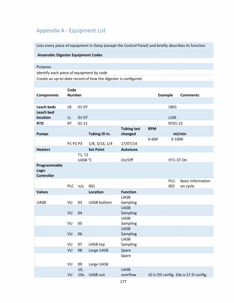
177
Appendix A - Equipment List
Lists every piece of equipment in Daisy (except the Control Panel) and briefly describes its function
Anaerobic Digester Equipment Codes
Purpose: Identify each piece of equipment by code Create an up-to-date record of how the digester is configured
Components Code Number Example Comments
Leach beds LB 01-07 LB01
Leach bed location LL 01-07 LL06 RTD RT 01-11 RT01-15
Pumps Tubing ID in. Tubing last changed
RPM ml/min
P1 P2 P3 1/8, 3/16, 1/4 17/07/14 0-600 0-1000
Heaters Set Point Autotune
T1, T2 UASB °C On/Off HT1-37-On
Programmable Logic Controller
PLC n/a 001
PLC-001
Basic information on cycle
Valves Location Function
UASB VU 03 UASB bottom UASB Sampling
VU 04 UASB Sampling
VU 05 UASB Sampling
VU 06 UASB Sampling
VU 07 UASB top UASB Sampling
VU 08 Large UASB Spare
VU 09 Large UASB
Spare
VU 10, 10a UASB out
UASB overflow 10 is 55l config. 10a is 27.5l config.

178
VU 11, 11a
UASB outlet drain
UASB sampling 11 is 55l config. 11a is 27.5l config.
VU 12 WW tank discharge
VU 13 UASB drain
VU 14 UASB isolation
VU 15 UASB fill/feed sample
Gas VG 01 LL-01 Open: GM1, Closed: GM2
VG 02 LL-01 Open: GM2, Closed: GM1
VG 03 LL-02 Open: GM1, Closed: GM2
VG 04 LL-02 Open: GM2, Closed: GM1
VG 05 LL-03 Open: GM1, Closed: GM2
VG 06 LL-04 Open: GM2, Closed: GM1
VG 07 LL-04 Open: GM1, Closed: GM2
VG 08 LL-05 Open: GM2, Closed: GM1
VG 09 LL-05 Open: GM1, Closed: GM2
VG 10 LL-06 Open: GM2, Closed: GM1
VG 11 LL-06 Open: GM1, Closed: GM2
VG 12 LL-07 Open: GM2, Closed: GM1
VG 13 LL-01 Gas sampling ports
VG 14 LL-02 Gas sampling ports
VG 15 LL-03 Gas sampling ports
VG 16 LL-04 Gas sampling ports
VG 17 LL-05 Gas sampling ports
VG 18 LL-06 Gas sampling ports
VG 19 Top UASB Open: UASB to GM2, Closed UASB to GM1
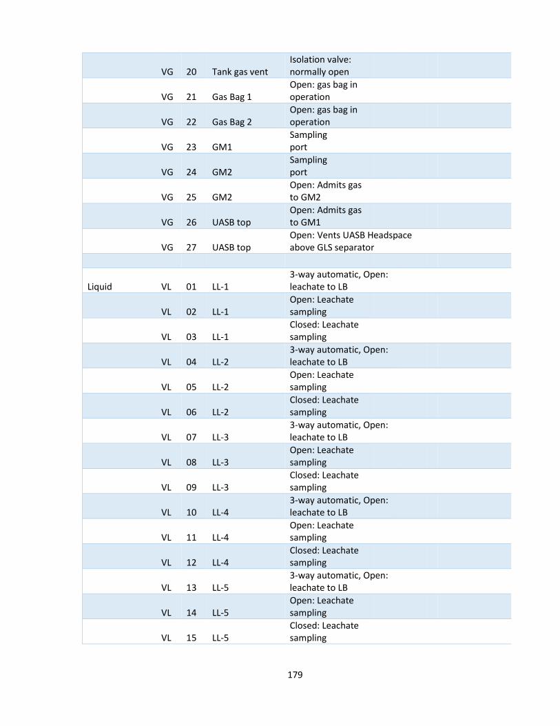
179
VG 20 Tank gas vent Isolation valve: normally open
VG 21 Gas Bag 1 Open: gas bag in operation
VG 22 Gas Bag 2 Open: gas bag in operation
VG 23 GM1 Sampling port
VG 24 GM2 Sampling port
VG 25 GM2 Open: Admits gas to GM2
VG 26 UASB top Open: Admits gas to GM1
VG 27 UASB top Open: Vents UASB Headspace above GLS separator
Liquid VL 01 LL-1 3-way automatic, Open: leachate to LB
VL 02 LL-1 Open: Leachate sampling
VL 03 LL-1 Closed: Leachate sampling
VL 04 LL-2 3-way automatic, Open: leachate to LB
VL 05 LL-2 Open: Leachate sampling
VL 06 LL-2 Closed: Leachate sampling
VL 07 LL-3 3-way automatic, Open: leachate to LB
VL 08 LL-3 Open: Leachate sampling
VL 09 LL-3 Closed: Leachate sampling
VL 10 LL-4 3-way automatic, Open: leachate to LB
VL 11 LL-4 Open: Leachate sampling
VL 12 LL-4 Closed: Leachate sampling
VL 13 LL-5 3-way automatic, Open: leachate to LB
VL 14 LL-5 Open: Leachate sampling
VL 15 LL-5 Closed: Leachate sampling

180
VL 16 LL-6 3-way automatic, Open: leachate to LB
VL 17 LL-6 Open: Leachate sampling
VL 18 LL-6 Closed: Leachate sampling
VL 19 Leachate drain manifold
Sampling, cleaning manifold
VL 20 Leach bed feed line
Sampling Leach bed feed
VL 21 Leach bed feed line
T2 Isolation valve, Closed for pressure testing
VL 22 UASB effluent line
Open: UASB effluent to T2 (with VL 23 closed)
VL 23 UASB effluent line
Open: UASB effluent to T1 (with VL 22 closed)
VL 24 T2-T1 transfer line (on T2)
Open: Allows leach bed effluent to go directly to T2 (with VP04 closed and P2 off)
VL 25 T1 Fill valve Allows liquid to be introduced to Tank 1
VL 26 T2 Fill valve Allows liquid to be introduced to Tank 2
Pump VP 01 UASB feed side of P1
Isolate pump for service
VP 02 T-1 side of P1 Isolate pump for service
VP 03 T-1 side of P2 Isolate pump for service
VP 04 T-2 side of P2 Isolate pump for service
VP 05 T-2 side of P3 Isolate pump for service
VP 06 Leach bed feed side of P3
Isolate pump for service
Quick disconnects VQ 1 LB-01 gas out
Re: and re: leach beds
VQ 2 LB-01 leachate in
Re: and re: leach beds
VQ 3 LB-01 leachate out
Re: and re: leach beds
VQ 4 LB-02 gas out Re: and re: leach beds
VQ 5 LB-02 leachate in
Re: and re: leach beds
VQ 6 LB-02 leachate out
Re: and re: leach beds
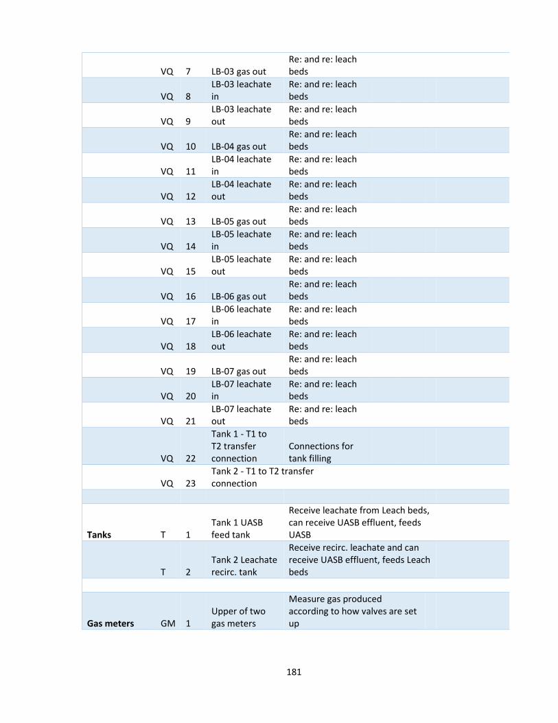
181
VQ 7 LB-03 gas out Re: and re: leach beds
VQ 8 LB-03 leachate in
Re: and re: leach beds
VQ 9 LB-03 leachate out
Re: and re: leach beds
VQ 10 LB-04 gas out Re: and re: leach beds
VQ 11 LB-04 leachate in
Re: and re: leach beds
VQ 12 LB-04 leachate out
Re: and re: leach beds
VQ 13 LB-05 gas out Re: and re: leach beds
VQ 14 LB-05 leachate in
Re: and re: leach beds
VQ 15 LB-05 leachate out
Re: and re: leach beds
VQ 16 LB-06 gas out Re: and re: leach beds
VQ 17 LB-06 leachate in
Re: and re: leach beds
VQ 18 LB-06 leachate out
Re: and re: leach beds
VQ 19 LB-07 gas out Re: and re: leach beds
VQ 20 LB-07 leachate in
Re: and re: leach beds
VQ 21 LB-07 leachate out
Re: and re: leach beds
VQ 22
Tank 1 - T1 to T2 transfer connection
Connections for tank filling
VQ 23 Tank 2 - T1 to T2 transfer connection
Tanks T 1 Tank 1 UASB feed tank
Receive leachate from Leach beds, can receive UASB effluent, feeds UASB
T 2 Tank 2 Leachate recirc. tank
Receive recirc. leachate and can receive UASB effluent, feeds Leach beds
Gas meters GM 1 Upper of two gas meters
Measure gas produced according to how valves are set up

182
GM 2 Lower of two gas meters
Measure gas produced according to how valves are set up
Foam Traps FT 1 Below GMs Capture any foam in the gas line ahead of GM1
FT 2 Below GMs Capture any foam in the gas line ahead of GM2
Gas Bags GB 1 Upper right of gas manifold
Compensate for liquid volumes withdrawn from the GM1 side of system
GB 2 Lower right of gas manifold
Compensate for liquid volumes withdrawn from the GM2 side of system
Switches Main Power SM Controls all power to digester Valve sequencer VS
Controls the valve sequencer for Leach beds
Leach bed switch LS
1 - 6
Controls the automatic valve to each LB - auto, closed, manual
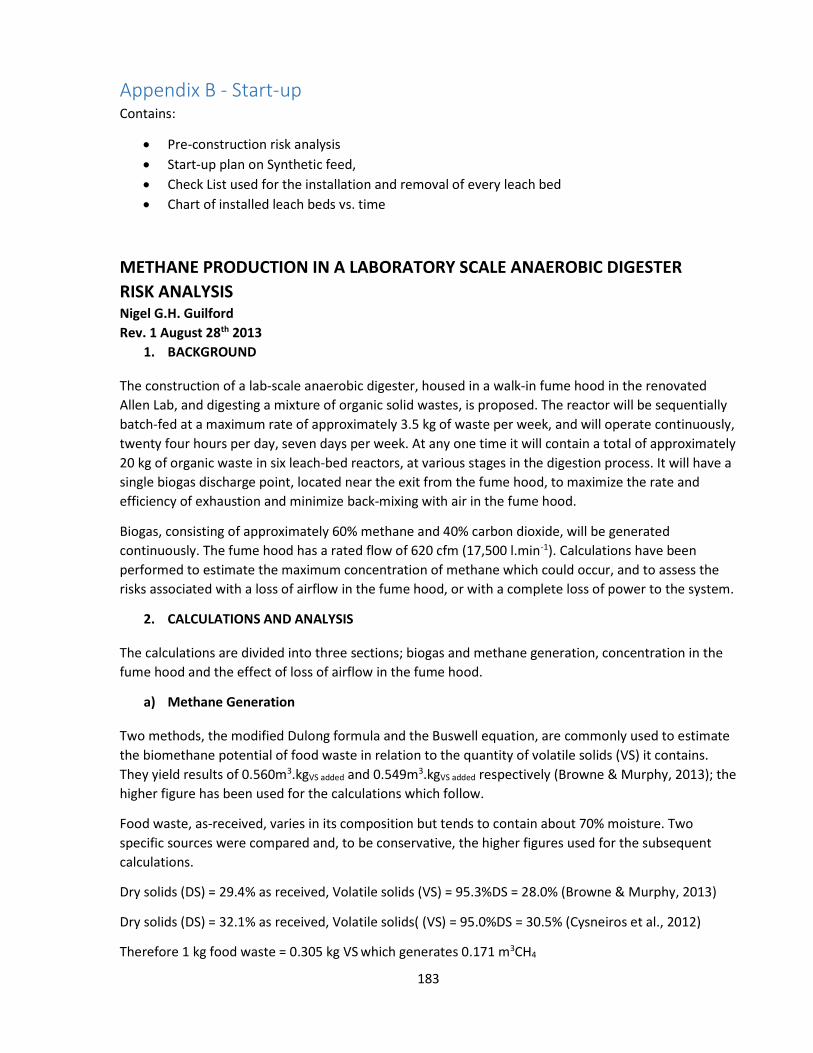
183
Appendix B - Start-up Contains:
Pre-construction risk analysis Start-up plan on Synthetic feed, Check List used for the installation and removal of every leach bed Chart of installed leach beds vs. time
METHANE PRODUCTION IN A LABORATORY SCALE ANAEROBIC DIGESTER RISK ANALYSIS Nigel G.H. Guilford Rev. 1 August 28th 2013
1. BACKGROUND
The construction of a lab-scale anaerobic digester, housed in a walk-in fume hood in the renovated Allen Lab, and digesting a mixture of organic solid wastes, is proposed. The reactor will be sequentially batch-fed at a maximum rate of approximately 3.5 kg of waste per week, and will operate continuously, twenty four hours per day, seven days per week. At any one time it will contain a total of approximately 20 kg of organic waste in six leach-bed reactors, at various stages in the digestion process. It will have a single biogas discharge point, located near the exit from the fume hood, to maximize the rate and efficiency of exhaustion and minimize back-mixing with air in the fume hood.
Biogas, consisting of approximately 60% methane and 40% carbon dioxide, will be generated continuously. The fume hood has a rated flow of 620 cfm (17,500 l.min-1). Calculations have been performed to estimate the maximum concentration of methane which could occur, and to assess the risks associated with a loss of airflow in the fume hood, or with a complete loss of power to the system.
2. CALCULATIONS AND ANALYSIS
The calculations are divided into three sections; biogas and methane generation, concentration in the fume hood and the effect of loss of airflow in the fume hood.
a) Methane Generation
Two methods, the modified Dulong formula and the Buswell equation, are commonly used to estimate the biomethane potential of food waste in relation to the quantity of volatile solids (VS) it contains. They yield results of 0.560m3.kgVS added and 0.549m3.kgVS added respectively (Browne & Murphy, 2013); the higher figure has been used for the calculations which follow.
Food waste, as-received, varies in its composition but tends to contain about 70% moisture. Two specific sources were compared and, to be conservative, the higher figures used for the subsequent calculations.
Dry solids (DS) = 29.4% as received, Volatile solids (VS) = 95.3%DS = 28.0% (Browne & Murphy, 2013)
Dry solids (DS) = 32.1% as received, Volatile solids( (VS) = 95.0%DS = 30.5% (Cysneiros et al., 2012)
Therefore 1 kg food waste = 0.305 kg VS which generates 0.171 m3CH4

184
Thus at a feed rate of 3.5 kg per week of food waste, the digester produces 0.6 m3CH4 (at 1 atm. and 250C) which is equivalent to:
Methane flow rates of:
3.6 l.hr-1 0.06 l.min-1 1.0 ml.s-1 6.5 x 10⁻⁴ g.s-1 (gram molecular volume = 24,465 ml.mole-1 and mwt. = 16)
b) Maximum Concentration in Fume Hood
The rated airflow is 620 cfm, or 17,500 l.min-1, (from the shop drawings of the new lab). Thus the 0.06 l.min-1 of methane generated is diluted with incoming air to 3.37 ppmv which, combined with a background atmospheric concentration of 1.79 ppmv (IPCC), gives:
Maximum methane concentration = 5.16 ppmv Since the lower explosive limit for methane is 5%,
Maximum methane concentration = 0.01% LEL
c) Effect of Power Failure or Fan Failure In the event of a power failure both the fume hood fan and the reactor will shut down; in these circumstances, four things must be considered:
i. Density of Methane Methane has a density of 55% of that of air that of air which, combined with the fact that the discharge point will be at the top of the fume hood near the exit, helps ensure continued venting of methane.
ii. Natural Draft Natural draft will maintain a slow airflow through the hood which, combined with the low density of methane and the elevated temperature in the system of 37OC (which, initially, will raise the temperature in the fume hood when the fan stops) will help ensure venting of methane to the outside, presumably the manner in which all hoods function during a power failure. The presence of a natural draft should be confirmed before the system becomes operational.
iii. Methane Production from the Digester Methane production will gradually begin to fall following an unplanned shutdown; but it will not cease immediately. However, the calculation below confirms that, even if methane production continued undiminished, and none was discharged under natural draft, it would take more than 60 hours for the concentration in the fume hood to reach the LEL. Volume of fume hood (from shop drawings) = 96” width x 90” height x 32” depth = 160 ft3 or 4,528 litres. Since the LEL is 5% by volume, or 226 litres, it would take 63 hrs to reach the LEL at a methane generation rate of 3.6 l.hr-1.

185
iv. Electrical Equipment
In the event of a power failure there is obviously no risk of an electrical spark. But, in the event of a fan failure without a general power failure, it would be prudent to provide for an automatic shutdown of the reactor. In both sets of circumstances the reactor controls will be designed to require a manual restart, in other words restoration of power will not restart the system without the operator present. A minimum of one hour of ventilation, following restoration of power and before system restart, should be part of the standard operating practice.
3. CONCLUSIONS
a) The risks associated with the generation and discharge of methane into a fume hood, have been shown to be negligible.
b) Tests should be performed to confirm that the system still draws air when the fume hood is not operational.
c) An interlock should be provided to shut the reactor down if the fan were to fail for any reason other than a power failure.
d) The system should be designed such that, after a shutdown, re-start is manual. e) One hour minimum of ventilation should follow restoration of power, before system restart.
UASB START-UP PLAN - November 2014
1. Objectives Start the UASB using a synthetic feedstock and anaerobic sludge as inoculum Run the system to observe methane production and the granulation of the sludge over time Substitute leachate from the leach beds for the synthetic feed once the UASB has become
stable and suitable for processing leachate
2. Operating conditions Campos and Anderson(Campos & Anderson, 1992) found that the best conditions for rapid start-up of a UASB on wastewater consisted of the following:
COD: 1000mg.l-1 rising to 2000mg.l-1 OLR: 2.0g.l-1.d-1 Vup: 0.05m.hr-1 rising to 0.1m.hr-1
UASB has a cross-sectional area of 500cm2 and is set up with an operating volume of 27.5l. Therefore, at Vup of 0.05m.hr-1 and feed concentration of 1000mgCOD.l-1,the HRT is 11h. and the OLR is 0.05 x 100 x 500 x 1 x 24/27.5 = 2.18gCOD.l-1.d-1. Raising Vup to 0.1m.hr-1 would result in an OLR of 4.36 gCOD.l-1.d-1, at the same concentration. Assuming the UASB is fed from T1 only (20L), at a flowrate of 2.5l.hr-1, and the effluent returned to T1, with a COD removal efficiency of 50%, 13.75g of COD should be added to T1 every 11 hours.

186
Assuming further that T2 is filled with make-up COD at 100x concentration (84g.l-1 of dissolved substrate), 137.5ml of concentrate must be added every 11 hours, or 300ml every 24 hours. This can be delivered from T2 by Pump 3 through LL01. Alternatively, both tanks (40l) can be filled with substrate, and concentrate added once per day to T2 and transferred to T1. This could be accomplished manually. The use of concentrate simplifies operation but requires a substrate concentration of 100gS COD.l-1 (83g.l-1 of substrate). Components other than the carbon source (minerals and trace elements) need only be topped up in proportion to the amount of effluent discharged.
3. Feedstock Feedstock will consist of the following
a) Carbon source comprising starch, carboxymethyl cellulose, protein and lipids b) Concentration of 1000mg SCOD.l-1 c) C:N ratio of around 28:1 d) Minerals, trace elements, vitamins, Resazurin
3.1 Carbon Source 4. From Guerrero, modified to include CMC carbon in place of half the starch carbon, (Guerrero et
al., 2009b) chose carbon supplied as follows: 5. Inoculum
Three steps
a) Sludge from Maryland Farms on-farm digester; a CSTR processing farm waste and food waste. Add 4-5 litres to the UASB, measure the COD.
b) Blend and squeeze some food waste, measure the TS/VS/COD, substitute for the carbon source above (subject to quantity considerations)
c) Start up the leach beds and replace the entire synthetic carbon source with leachate.
6. System Start-up
a) Drain tanks and fill with DI water b) Add 0.5 g.l-1 sucrose to system (34g) and circulate T2 – T1 – UASB – T2 c) Drain 4.5 litres from UASB d) Drain 3.0 litres from T2 e) Flush entire system with argon f) Add to T2
i. 670 ml substrate concentrate ii. 670 ml MM1
iii. 670 ml MM2 (modified) iv. 134 ml MM3 v. 134 ml MM4
vi. 67 ml MM5 vii. 670 ml MM6
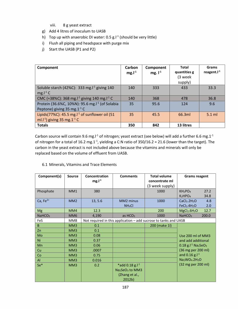
187
viii. 8 g yeast extract g) Add 4 litres of inoculum to UASB h) Top up with anaerobic DI water: 0.5 g.l-1 (should be very little) i) Flush all piping and headspace with purge mix j) Start the UASB (P1 and P2)
Component Carbon mg.l-1
Component mg. l-1
Total quantities g
(3 week supply)
Grams reagent.l-1
Soluble starch (42%C): 333 mg.l-1 giving 140 mg.l-1 C
140 333 433 33.3
CMC (≈38%C): 368 mg.l-1 giving 140 mg.l-1 C 140 368 478 36.8 Protein (36.6%C, 10%N): 95.6 mg.l-1 (of Solabia Peptone) giving 35 mg.1-1 C
35 95.6 124 9.6
Lipids(77%C): 45.5 mg.l-1 of sunflower oil (51 ml.l-1) giving 35 mg.1-1 C
35 45.5 66.3ml 5.1 ml
Totals 350 842 13 litres Carbon source will contain 9.6 mg.l-1 of nitrogen; yeast extract (see below) will add a further 6.6 mg.1-1 of nitrogen for a total of 16.2 mg.1-1, yielding a C:N ratio of 350/16.2 = 21.6 (lower than the target). The carbon in the yeast extract is not included above because the vitamins and minerals will only be replaced based on the volume of effluent from UASB.
6.1 Minerals, Vitamins and Trace Elements
Component(s) Source Concentration mg.l-1
Comments Total volume concentrate ml
(3 week supply)
Grams reagent
Phosphate MM1 380 1000 KH2PO4 27.2 K2HPO4 34.8
Ca, Fe2+ MM2 13, 5.6 MM2 minus NH4Cl
1000 CaCl2.2H2O 4.8 FeCl2.4H2O 2.0
Mg MM4 12.3 200 MgCl2.6H2O 12.7 NaHCO3 MM6 4,190 as HCO3
1000 NaHCO3 200.0 FeS MM8 Not required in this application – add sucrose to tanks and UASB B MM3 0.1 200 (make 1l)
Use 200 ml of MM3 and add additional 0.18 g.l-1 Na2SeO3 (36 mg per 200 ml) and 0.16 g.l-1 Na2WO4.2H2O (32 mg per 200 ml)
Zn MM3 0.1 Mo MM3 0.08 Ni MM3 0.37 Mn MM3 0.06 Cu MM3 .0007 Co MM3 0.75 Al MM3 0.016 Se* MM3 0.2 *add 0.18 g.l-1
Na2SeO3 to MM3 (Zhang et al.,
2012b)

188
W* MM3 0.2 add 0.16 g.l-1 Na2WO4 to MM3
(Zhang et al., 2012b)
Vitamins Yeast extract
100 mg.l-1 Contributes 6.6 mg.l-1 of nitrogen
(Carnicer et al., 2009)
8 grams 8.0
Resazurin MM5 1.0 100 100 ml
Leach Bed Removal, Filling and Installation Checklist Date: LB Removal LL LB S: LB Installation LL LB S:
Removal - Day 1
Step Task Complete 1 Write up sched. of LB contents FB FW BA LY water/LT
2 Sample VU15 1x15ml (TS/VS/COD), 1x50ml (pH/alk.), 1x10 ml (VFAs)
3 Record LT levels in T1 and T2. Top up T2 if necessary - record vol. added
4 Close LB Switch: Control panel
5 Close VL Drain 30 min
6 Allow LT to accum.and take 1x15ml sample 7 Remove LB and weigh: 8 Place on stand with vents inserted;

189
Installation - Day 1 Step Task Complete
9 Move FW from freezer to walk-in fridge (at least 24hr in advance)
10 Dry BA in oven (2 days in advance) or measure TS and correct weight BA
11 Bring FW to room temp 12 Weigh out FB and BA into two buckets (50:50) 13 Add water, half to each bucket, and mix 14 Prep FW (remove foreign matter) 15 Weigh out FW plus equal weight water and mix 16 Retain some water to rinse food waste into bucket 17 Prep. coupons (if any) 18 Gross wt. of coupons = g 19 Add FW to FB; mix thoroughly 20 Tare LB: 21 Install geotextile and overflow 22 Load waste, tamp down by hand to an even density 23 Load coupons (if any) and record depth of placement 24 Place upper geotextile - line up hole with RTD location 25 Measure freeboard 26 Place O-ring and close LB; use prodder to create path for RTD 27 Insert RTD and tighten fitting 28 Tighten bottom flange lightly (if necessary) 29 Weigh LB: 30 Leak test fittings using argon and Snoop 31 Flush headspace with argon 32 Pressurize to @50cm water (use manometer to measure) 33 Install LB, open VL , Switch LB to Auto, 34 Record ΔP GM1 = cm GM2 = cm 35 Adjust setting for LB heater; record in daily log 36 Record time of completion 37

190
Removal - Day 2 Step Task Complete 38 Collect leachate overnight 39 Measure and record LT vol., return to T1 40 Re-weigh LB: 41 Weigh Al dishes for coupons 42 Gross wt. coupons out = g 43 Remove RTD from fitting carefully - clean with dil. HCl 44 Open LB S: 45 Measure freeboard and record any observations 46 Remove overflow, insert prodder with sample-height marks 47 Take samples (50ml) for microbio at 4cm intervals 48 Remove DG and retain samples at -13cm, -20cm, -25 cm and -28cm 49 Remove coupons (if any) for further analysis 50 Retain 300 - 500g DG in Ziploc bag put in freezer 51 Remove geotextiles, overflow, SS mesh 52 Retain remainder of DG for aerobic curing (store in cold room) 53 Wash everything thoroughly (soak geotextiles in detegent) and dry 54 Place cleaned LB on stand with vents inserted top and bottom

191
Leach Beds Installed versus Time Week Start End LL01 LL02 LL03 LL04 LL05 LL06
6 4/28/2015 5/4/2015 S.007 S.008 S.009 S.004 S.005 S.006
7 5/5/2015 5/11/2015 S.007 S.008 S.009 S.010 S.005 S.006
8 5/12/2015 5/18/2015 S.007 S.008 S.009 S.010 S.005 S.006
9 5/19/2015 5/25/2015 S.007 S.008 S.009 S.010 S.011 S.012
10 5/26/2015 6/1/2015 S.013 S.008 S.009 S.010 S.011 S.012
11 6/2/2015 6/8/2015 S.013 S.014 S.009 S.010 S.011 S.012
12 6/9/2015 6/15/2015 S.013 S.014 S.015 S.010 S.011 S.012
13 6/16/2015 6/22/2015 S.013 S.014 S.015 S.016 S.011 S.012
14 6/23/2015 6/29/2015 S.013 S.014 S.015 S.016 S.017 S.012
15 6/30/2015 7/6/2015 S.013 S.014 S.015 S.016 S.017 S.012
16 7/7/2015 7/13/2015 S.013 S.014 S.015 S.016 S.017 S.018
17 7/14/2015 7/20/2015 S.019 S.014 S.015 S.016 S.017 S.018
18 7/21/2015 7/27/2015 S.019 S.020 S.015 S.016 S.017 S.018
19 7/28/2015 8/3/2015 S.019 S.020 S.021 S.016 S.017 S.018
20 8/4/2015 8/10/2015 S.019 S.020 S.021 S.022 S.017 S.018
21 8/11/2015 8/17/2015 S.019 S.020 S.021 S.022 S.023 S.018
22 8/18/2015 8/24/2015 S.019 S.020 S.021 S.022 S.023 S.018
23 8/25/2015 8/31/2015 S.019 S.020 S.021 S.022 S.023 S.024
24 9/1/2015 9/7/2015 S.019 S.020 S.021 S.022 S.023 S.024
25 9/8/2015 9/14/2015 S.019 S.020 S.021 S.022 S.023 S.024
26 9/15/2015 9/21/2015 S.025 S.020 S.021 S.022 S.023 S.024
27 9/22/2015 9/28/2015 S.025 S.026 S.021 S.022 S.023 S.024
28 9/29/2015 10/5/2015 S.025 S.026 S.027 S.022 S.023 S.024
29 10/6/2015 10/12/2015 S.025 S.026 S.027 S.028 S.023 S.024
30 10/13/2015 10/19/2015 S.025 S.026 S.027 S.028 S.029 S.024
31 10/20/2015 10/26/2015 S.025 S.026 S.027 S.028 S.029 S.030
32 10/27/2015 11/2/2015 S.031 S.026 S.027 S.028 S.029 S.030
33 11/3/2015 11/9/2015 S.031 S.032 S.027 S.028 S.029 S.030
34 11/10/2015 11/16/2015 S.031 S.032 S.033 S.028 S.029 S.030
35 11/17/2015 11/23/2015 S.031 S.032 S.033 S.034 S.029 S.030
36 11/24/2015 11/30/2015 S.031 S.032 S.033 S.034 S.035 S.030
37 12/1/2015 12/7/2015 S.031 S.032 S.033 S.034 S.035 S.036
38 12/8/2015 12/14/2015 S.037 S.032 S.033 S.034 S.035 S.036
39 12/15/2015 12/21/2015 S.037 S.038 S.033 S.034 S.035 S.036
40 12/22/2015 12/28/2015 S.037 S.038 S.039 S.034 S.035 S.036
41 12/29/2015 1/4/2016 S.037 S.038 S.039 S.040 S.035 S.036
42 1/5/2016 1/11/2016 S.037 S.038 S.039 S.040 S.041 S.036
43 1/12/2016 1/18/2016 S.037 S.038 S.039 S.040 S.041 S.042
44 1/19/2016 1/25/2016 S.043 S.038 S.039 S.040 S.041 S.042
45 1/26/2016 2/1/2016 S.043 S.044 S.039 S.040 S.041 S.042
46 2/2/2016 2/8/2016 S.043 S.044 S.045 S.040 S.041 S.042
47 2/9/2016 2/15/2016 S.043 S.044 S.045 S.046 S.041 S.042

192
48 2/16/2016 2/22/2016 S.043 S.044 S.045 S.046 S.047 S.042
49 2/23/2016 2/29/2016 S.043 S.044 S.045 S.046 S.047 S.048
50 2016/03/01 2016/03/07 S.049 S.044 S.045 S.046 S.047 S.048
51 2016/03/08 2016/03/14 S.049 S.050 S.045 S.046 S.047 S.048
52 2016/03/15 2016/03/21 S.049 S.050 S.051 S.046 S.047 S.048
53 2016/03/22 2016/03/28 S.049 S.050 S.051 S.052 S.047 S.048
54 2016/03/29 2016/04/04 S.049 S.050 S.051 S.052 S.053 S.048
55 2016/04/05 2016/04/11 S.049 S.050 S.051 S.052 S.053 S.054
56 2016/04/12 2016/04/18 S.055 S.050 S.051 S.052 S.053 S.054
57 2016/04/19 2016/04/25 S.055 S.056 S.051 S.052 S.053 S.054
58 2016/04/26 2016/05/02 S.055 S.056 S.057 S.052 S.053 S.054
59 2016/05/03 2016/05/09 S.055 S.056 S.057 S.058 S.053 S.054
60 2016/05/10 2016/05/16 S.055 S.056 S.057 S.058 S.059 S.054
61 2016/05/17 2016/05/23 S.055 S.056 S.057 S.058 S.059 S.060
62 2016/05/24 2016/05/30 S.061 S.056 S.057 S.058 S.059 S.060
63 2016/05/31 2016/06/06 S.061 S.062 S.057 S.058 S.059 S.060
64 2016/06/07 2016/06/13 S.061 S.062 S.063 S.058 S.059 S.060
65 2016/06/14 2016/06/20 S.061 S.062 S.063 S.064 S.059 S.060
66 2016/06/21 2016/06/27 S.061 S.062 S.063 S.064 S.065 S.060
67 2016/06/28 2016/07/04 S.061 S.062 S.063 S.064 S.065 S.066
68 2016/07/05 2016/07/11 S.067 S.062 S.063 S.064 S.065 S.066
69 2016/07/12 2016/07/18 S.067 S.068 S.063 S.064 S.065 S.066
70 2016/07/19 2016/07/25 S.067 S.068 S.069 S.064 S.065 S.066
71 2016/07/26 2016/08/01 S.067 S.068 S.069 S.070 S.065 S.066
72 2016/08/02 2016/08/08 S.067 S.068 S.069 S.070 S.071 S.066
73 2016/08/09 2016/08/15 S.067 S.068 S.069 S.070 S.071 S.072
74 2016/08/16 2016/08/22 S.073 S.068 S.069 S.070 S.071 S.072
75 2016/08/23 2016/08/29 S.073 S.074 S.069 S.070 S.071 S.072
76 2016/08/30 2016/09/05 S.073 S.074 S.075 S.070 S.071 S.072
77 2016/09/06 2016/09/12 S.073 S.074 S.075 S.076 S.071 S.072
78 2016/09/13 2016/09/19 S.073 S.074 S.075 S.076 S.077 S.072
79 2016/09/20 2016/09/26 S.073 S.074 S.075 S.076 S.077 S.078
80 2016/09/27 2016/10/03 S.079 S.074 S.075 S.076 S.077 S.078
81 2016/10/04 2016/10/10 S.079 S.080 S.075 S.076 S.077 S.078
82 2016/10/11 2016/10/17 S.079 S.080 S.081 S.076 S.077 S.078
83 2016/10/18 2016/10/24 S.079 S.080 S.081 S.082 S.077 S.078
84 2016/10/25 2016/10/31 S.079 S.080 S.081 S.082 S.083 S.078
85 2016/11/01 2016/11/07 S.079 S.080 S.081 S.082 S.083 S.084
86 2016/11/08 2016/11/14 S.085 S.080 S.081 S.082 S.083 S.084
87 2016/11/15 2016/11/21 S.085 S.086 S.081 S.082 S.083 S.084
88 2016/11/22 2016/11/28 S.085 S.086 S.087 S.082 S.083 S.084
17.2%CODFW 12.9%CODFW 7.9%CODFW Zero%CODFW 21.7%CODFW 29.3%CODFW 17.2%CODFW 7wk. SRT
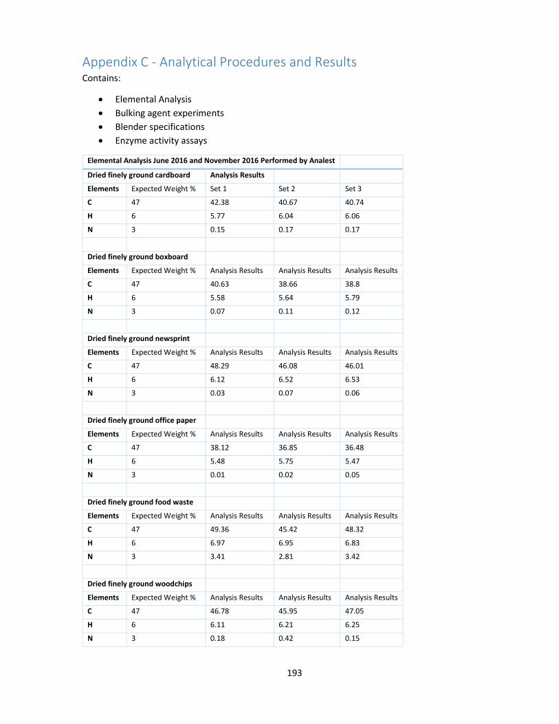
193
Appendix C - Analytical Procedures and Results Contains:
Elemental Analysis Bulking agent experiments Blender specifications Enzyme activity assays
Elemental Analysis June 2016 and November 2016 Performed by Analest
Dried finely ground cardboard Analysis Results
Elements Expected Weight % Set 1 Set 2 Set 3
C 47 42.38 40.67 40.74
H 6 5.77 6.04 6.06
N 3 0.15 0.17 0.17
Dried finely ground boxboard
Elements Expected Weight % Analysis Results Analysis Results Analysis Results
C 47 40.63 38.66 38.8
H 6 5.58 5.64 5.79
N 3 0.07 0.11 0.12
Dried finely ground newsprint
Elements Expected Weight % Analysis Results Analysis Results Analysis Results
C 47 48.29 46.08 46.01
H 6 6.12 6.52 6.53
N 3 0.03 0.07 0.06
Dried finely ground office paper
Elements Expected Weight % Analysis Results Analysis Results Analysis Results
C 47 38.12 36.85 36.48
H 6 5.48 5.75 5.47
N 3 0.01 0.02 0.05
Dried finely ground food waste
Elements Expected Weight % Analysis Results Analysis Results Analysis Results
C 47 49.36 45.42 48.32
H 6 6.97 6.95 6.83
N 3 3.41 2.81 3.42
Dried finely ground woodchips
Elements Expected Weight % Analysis Results Analysis Results Analysis Results
C 47 46.78 45.95 47.05
H 6 6.11 6.21 6.25
N 3 0.18 0.42 0.15

194
Aug/22/2016 Samples TKN Sample 1 CB Cardboard 0.167±0.005% Sample 2 BB Boxboard 0.111±0.002% Sample 3 NP Newsprint 0.062±0.001% Sample 4 FP Fine paper 0.043±0.005% Sample 5 FW Food waste 3.31±0.01% Sample 6 BA Woodchips 0.148±0.002% All are duplicate measurements.
May/05/2016 Samples TKN Sample 1 CB Cardboard 0.165±0.006% Sample 2 BB Boxboard 0.111±0.001% Sample 3 NP Newsprint 0.057±0.003% Sample 4 FP Fine paper 0.022±0.001% Sample 5 FW Food waste 2.66±0.01% Sample 6 BA Woodchips 0.379±0.001% All are duplicate measurements.
Bulking Agent Properties Experiments
Three simple experiments were conducted to compare the physical properties of two different shipments of bulking agent BA4 and BA5; particle size distribution, bulk density and water absorption capacity.
1. Particle Size Distribution
Duplicate dried samples of each bulking agent were screened at 3.36 mm 0.5 mm and 0.21 mm giving four fractions.
2. Bulk density
One litre beakers were filled loosely with duplicate dried samples of each bulking agent and weighed to determine specific gravity.
3. Water Absorption Capacity
Duplicate 50 g samples of dried bulking agent were weighed into 1 L beakers. 400 mL of DI water was added to each, the beaker covered, and left at room temperature for three days. The contents of each beaker in turn were discharged onto a pre-wet and 0.21 mm sieve with tared pan, and left to drain for one hour. The pan and its contents were weighed and the amount of water retained by the bulking agent calculated.

195
Blender Specifications
The blender used was a Blendtec Wildside with a 3hp motor; the blade is blunt, relying on impact and
shear. It has eight preset speeds and each cycle is 50 seconds long. The initial homogenizing was carried
out in a single cycle at sSeed 1 (the lowest).
Protocols for Enzyme Activity Assay
SDS Page
Enzyme samples were mixed 1:1 with 2x sample loading buffer (100mM Tris pH6.8, 10% SDS, 20% glycerol, 25% B-mercaptoethanol, 0.05% bromphenol blue) and heated to 95C for 10min. 20ul samples were loaded onto a 10% SDS polyacrylamide gel and run for 1h at 165V in 25mM Tris-HCl, 200mM glycine, 0.1% SDS running buffer. The gel was rinsed 3x with water and stained with Coomassie blue stain (40mg Brilliant Blue R, 3ml 6N HCl and water to 500ml) by covering gel in about 10-20ml satin, microwaving for 1min and shaking for 15min. Destain with water.
Bradford
Dilute Biorad Bradford concentrate 1:5 with water. Pipet 200ul into duplicate wells of a 96 well plate; 1 for each enzyme sample and 7 for the standard curve. For the standard curve add 0, 1, 1.5, 2, 2.5, 3, and 3.5ul of 1ug/ul BSA standard from Sigma. Added 10-20ul of enzyme samples. Mix by pipetting and read plate at 595nm. Prepared standard curve in Excel spreadsheet and used to determine protein concentration of samples.
Esterase
In duplicate, 50ul enzyme samples (including a blank) pipeted into wells of 96 well plate. Add 150ul reaction mix containing: 50mM HEPES pH7.5, 1.5mM 1-naphthyl acetate. Incubate at 37C for 1h. Read plate at 310nm. Subtract blank.
Proteinase
In duplicate, 50ul enzyme samples (including a blank) pipeted into wells of 96 well plate. Add 150ul reaction mix containing: 50mM HEPES, pH7.5, 5mM MgCl, 0.5mM MnCl, 0.5mM ZnCl, 0.5mM CaCl and 0.8mM each BAPNA, Leu-pNA, Pro-pNA, Suc-AAA-pNA and Suc-Phe-pNA. Incubate at 37C for 1h. Read plate at 410nm. Subtract blank.
Cellulase
In duplicate, 50ul enzyme samples (including a blank) pipeted into wells of 96 well plate. Add 150ul reaction mix containing: 50mM HEPES, pH7.5 and 2mM each pNP-B-D cellobioside, pNP-a-D maltoside and pNP-B-D maltoside. Incubate at 37C for 1h. Read plate at 410nm. Subtract blank. The cellobioside is a general substrate for exo-cellulases (exo-gluconases). The maltosides are also for exo-gluconases but are more specific (they also detect amylases – starch degrading glycoside hydrolases).

196
Appendix D - Operating Results Contains:
Digestate Properties COD mass balance for each leach bed one Table for each Period Substrate destruction efficiency by leach bed one Table for each Period (except Period
1 which is in the main body of the thesis Coupon STDEV table of n values BMP2 Substrate destruction efficiency calculations Leach bed permeability tests
Moisture TS VS/TS DG COD
LB Serial # Period % [g dry/g DG] [g VS/g DG] [g COD/g DG] 1
1
78.8% 0.21 0.89 1.21 2 78.8% 0.21 0.86 1.18 3 78.5% 0.22 0.87 1.19 4 79.2% 0.21 0.81 1.10 5 79.5% 0.21 0.82 1.12 6 78.9% 0.21 0.83 1.13 7 79.6% 0.20 0.83 1.13 8 78.2% 0.22 0.85 1.16 9 78.6% 0.21 0.86 1.16
10 78.1% 0.22 0.86 1.16 11 78.5% 0.22 0.86 1.17 12 78.9% 0.21 0.83 1.13 13 79.1% 0.21 0.84 1.15 14 78.4% 0.22 0.84 1.14 15 78.0% 0.22 0.85 1.16 16 77.6% 0.22 0.85 1.16 17
2
76.9% 0.23 0.86 1.17 18 77.6% 0.22 0.86 1.17 19 78.0% 0.22 0.86 1.18 20 77.3% 0.23 0.85 1.14 21 77.4% 0.23 0.81 1.12 22 77.0% 0.23 0.83 1.13 23 77.3% 0.23 0.82 1.17 24 77.2% 0.23 0.82 1.17 25
3
76.2% 0.24 0.81 1.16 26 77.4% 0.23 0.82 1.16 27 76.5% 0.23 0.83 1.16 28 77.1% 0.23 0.83 1.13 29 77.4% 0.23 0.84 1.13 30 76.5% 0.24 0.84 1.14 31
4a
76.6% 0.23 0.87 1.17 32 76.4% 0.24 0.86 1.22 33 76.7% 0.23 0.86 1.17 34 76.1% 0.24 0.86 1.13 35 75.7% 0.24 0.87 1.17 36 75.6% 0.24 0.86 1.16 37
4b
75.7% 0.24 0.87 1.13 38 75.2% 0.25 0.87 1.18 39 73.6% 0.26 0.90 1.17 40 74.4% 0.26 0.89 1.18 41 75.0% 0.25 0.89 1.16 42 73.5% 0.27 0.91 1.17
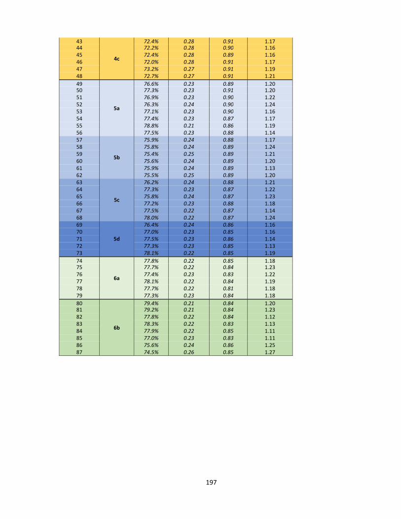
197
43
4c
72.4% 0.28 0.91 1.17 44 72.2% 0.28 0.90 1.16 45 72.4% 0.28 0.89 1.16 46 72.0% 0.28 0.91 1.17 47 73.2% 0.27 0.91 1.19 48 72.7% 0.27 0.91 1.21 49
5a
76.6% 0.23 0.89 1.20 50 77.3% 0.23 0.91 1.20 51 76.9% 0.23 0.90 1.22 52 76.3% 0.24 0.90 1.24 53 77.1% 0.23 0.90 1.16 54 77.4% 0.23 0.87 1.17 55 78.8% 0.21 0.86 1.19 56 77.5% 0.23 0.88 1.14 57
5b
75.9% 0.24 0.88 1.17 58 75.8% 0.24 0.89 1.24 59 75.4% 0.25 0.89 1.21 60 75.6% 0.24 0.89 1.20 61 75.9% 0.24 0.89 1.13 62 75.5% 0.25 0.89 1.20 63
5c
76.2% 0.24 0.88 1.21 64 77.3% 0.23 0.87 1.22 65 75.8% 0.24 0.87 1.23 66 77.2% 0.23 0.88 1.18 67 77.5% 0.22 0.87 1.14 68 78.0% 0.22 0.87 1.24 69
5d
76.4% 0.24 0.86 1.16 70 77.0% 0.23 0.85 1.16 71 77.5% 0.23 0.86 1.14 72 77.3% 0.23 0.85 1.13 73 78.1% 0.22 0.85 1.19 74
6a
77.8% 0.22 0.85 1.18 75 77.7% 0.22 0.84 1.23 76 77.4% 0.23 0.83 1.22 77 78.1% 0.22 0.84 1.19 78 77.7% 0.22 0.81 1.18 79 77.3% 0.23 0.84 1.18 80
6b
79.4% 0.21 0.84 1.20 81 79.2% 0.21 0.84 1.23 82 77.8% 0.22 0.84 1.12 83 78.3% 0.22 0.83 1.13 84 77.9% 0.22 0.85 1.11 85 77.0% 0.23 0.83 1.11 86 75.6% 0.24 0.86 1.25 87 74.5% 0.26 0.85 1.27
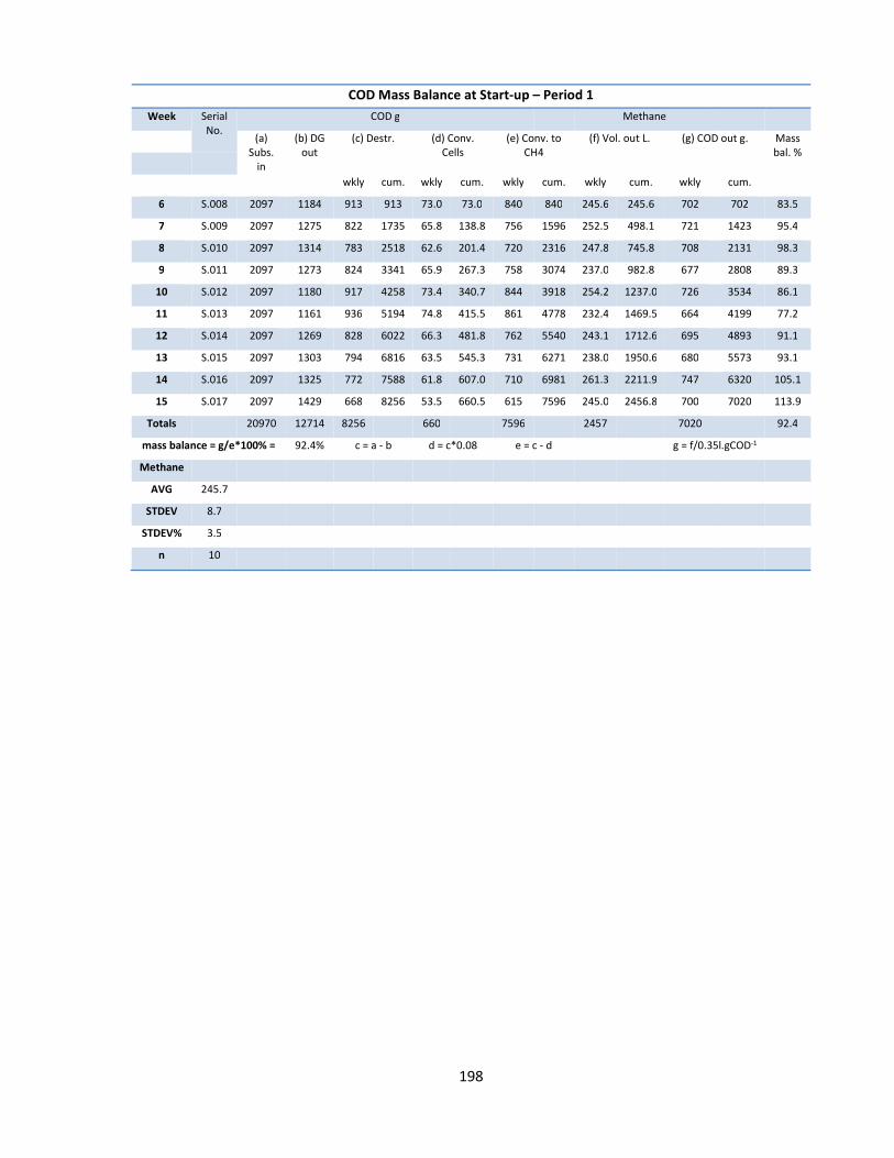
198
COD Mass Balance at Start-up – Period 1 Week Serial
No. COD g
Methane
(a)
Subs. in
(b) DG out
(c) Destr. (d) Conv. Cells
(e) Conv. to CH4
(f) Vol. out L. (g) COD out g. Mass bal. %
wkly cum. wkly cum. wkly cum. wkly cum. wkly cum.
6 S.008 2097 1184 913 913 73.0 73.0 840 840 245.6 245.6 702 702 83.5
7 S.009 2097 1275 822 1735 65.8 138.8 756 1596 252.5 498.1 721 1423 95.4
8 S.010 2097 1314 783 2518 62.6 201.4 720 2316 247.8 745.8 708 2131 98.3
9 S.011 2097 1273 824 3341 65.9 267.3 758 3074 237.0 982.8 677 2808 89.3
10 S.012 2097 1180 917 4258 73.4 340.7 844 3918 254.2 1237.0 726 3534 86.1
11 S.013 2097 1161 936 5194 74.8 415.5 861 4778 232.4 1469.5 664 4199 77.2
12 S.014 2097 1269 828 6022 66.3 481.8 762 5540 243.1 1712.6 695 4893 91.1
13 S.015 2097 1303 794 6816 63.5 545.3 731 6271 238.0 1950.6 680 5573 93.1
14 S.016 2097 1325 772 7588 61.8 607.0 710 6981 261.3 2211.9 747 6320 105.1
15 S.017 2097 1429 668 8256 53.5 660.5 615 7596 245.0 2456.8 700 7020 113.9
Totals
20970 12714 8256
660
7596
2457
7020
92.4
mass balance = g/e*100% = 92.4% c = a - b d = c*0.08 e = c - d
g = f/0.35l.gCOD-1
Methane
AVG 245.7
STDEV 8.7
STDEV% 3.5
n 10
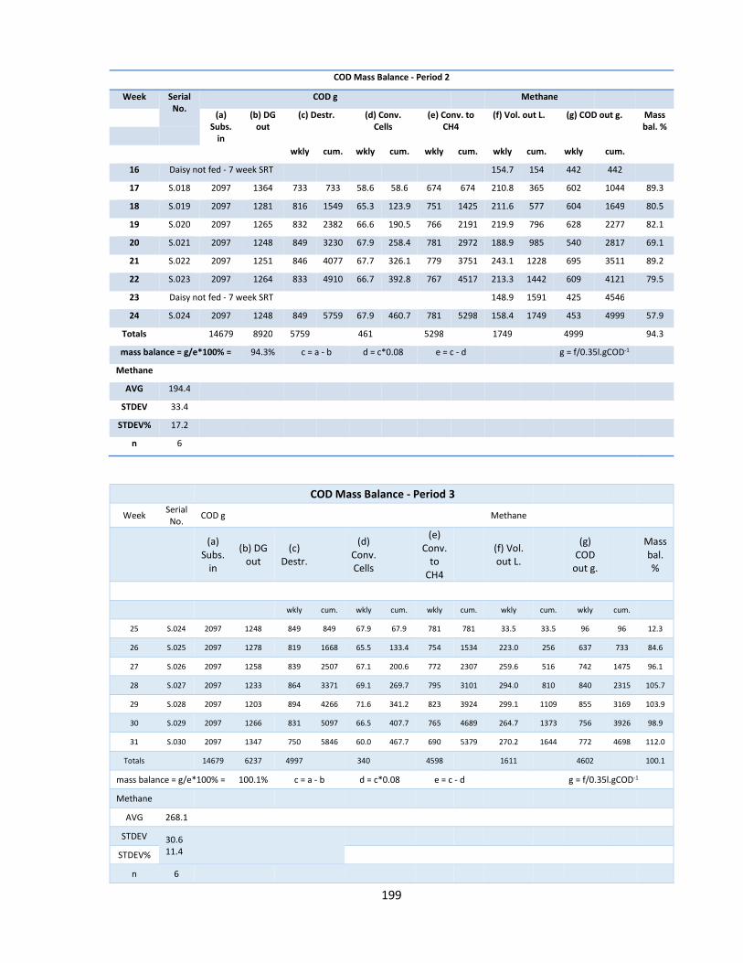
199
COD Mass Balance - Period 2
Week Serial No.
COD g
Methane
(a)
Subs. in
(b) DG out
(c) Destr. (d) Conv. Cells
(e) Conv. to CH4
(f) Vol. out L. (g) COD out g. Mass bal. %
wkly cum. wkly cum. wkly cum. wkly cum. wkly cum.
16 Daisy not fed - 7 week SRT
154.7 154 442 442
17 S.018 2097 1364 733 733 58.6 58.6 674 674 210.8 365 602 1044 89.3
18 S.019 2097 1281 816 1549 65.3 123.9 751 1425 211.6 577 604 1649 80.5
19 S.020 2097 1265 832 2382 66.6 190.5 766 2191 219.9 796 628 2277 82.1
20 S.021 2097 1248 849 3230 67.9 258.4 781 2972 188.9 985 540 2817 69.1
21 S.022 2097 1251 846 4077 67.7 326.1 779 3751 243.1 1228 695 3511 89.2
22 S.023 2097 1264 833 4910 66.7 392.8 767 4517 213.3 1442 609 4121 79.5
23 Daisy not fed - 7 week SRT
148.9 1591 425 4546
24 S.024 2097 1248 849 5759 67.9 460.7 781 5298 158.4 1749 453 4999 57.9
Totals
14679 8920 5759
461
5298
1749
4999
94.3
mass balance = g/e*100% = 94.3% c = a - b d = c*0.08 e = c - d
g = f/0.35l.gCOD-1
Methane
AVG 194.4
STDEV 33.4
STDEV% 17.2
n 6
COD Mass Balance - Period 3
Week Serial No.
COD g Methane
(a)
Subs. in
(b) DG out
(c) Destr.
(d)
Conv. Cells
(e)
Conv. to
CH4
(f) Vol. out L.
(g)
COD out g.
Mass bal. %
wkly cum. wkly cum. wkly cum. wkly cum. wkly cum.
25 S.024 2097 1248 849 849 67.9 67.9 781 781 33.5 33.5 96 96 12.3
26 S.025 2097 1278 819 1668 65.5 133.4 754 1534 223.0 256 637 733 84.6
27 S.026 2097 1258 839 2507 67.1 200.6 772 2307 259.6 516 742 1475 96.1
28 S.027 2097 1233 864 3371 69.1 269.7 795 3101 294.0 810 840 2315 105.7
29 S.028 2097 1203 894 4266 71.6 341.2 823 3924 299.1 1109 855 3169 103.9
30 S.029 2097 1266 831 5097 66.5 407.7 765 4689 264.7 1373 756 3926 98.9
31 S.030 2097 1347 750 5846 60.0 467.7 690 5379 270.2 1644 772 4698 112.0
Totals 14679 6237 4997 340 4598 1611 4602 100.1
mass balance = g/e*100% = 100.1% c = a - b d = c*0.08 e = c - d g = f/0.35l.gCOD-1
Methane
AVG 268.1
STDEV 30.6 11.4
STDEV%
n 6

200
COD Mass Balance - Period 4
Week Serial No. COD g Methane
(a)
Subs. in
(b) DG out
(c) Destr.
(d) Conv. Cells
(e)
Conv. to CH4
(f) Vol. out L.
(g) COD out g. Mass bal. %
wkly cum. wkly cum. wkly cum. wkly cum. wkly cum.
32 S.030 2097 1347 749 749 59.9 59.9 689 689 225.9 225.9 645 645 93.6
33 S.031 2024 1425 600 1349 48.0 107.9 552 1241 198.4 424.3 567 1212 102.8
34 S.032 2024 1497 527 1876 42.2 150.1 485 1726 196.9 621.2 563 1775 116.0
35 S.033 2024 1397 627 2503 50.2 200.3 577 2303 206.3 827.5 590 2364 102.2
36 S.034 2024 1343 682 3185 54.6 254.8 627 2930 193.6 1021.2 553 2918 88.2
37 S.035 2024 1468 556 3742 44.5 299.3 512 3442 193.2 1214.3 552 3470 107.8
Totals 12219 8477 3741 299.3 3442 1214.3 3469 100.8
38 S.036 2024 1485 539 539 43.1 43.1 496 496 169.5 169.5 484 484 97.6
39 S.037 1950 1404 547 1086 43.7 86.9 503 999 161.0 330.6 460 944 91.4
40 S.038 1950 1482 469 1555 37.5 124.4 431 1430 142.0 472.5 406 1350 94.1
41 S.039 1950 1576 375 1929 30.0 154.3 345 1775 135.0 607.5 386 1736 112.0
42 S.040 1950 1533 418 2347 33.4 187.8 384 2159 138.4 745.9 395 2131 102.9
43 S.041 1950 1489 461 2808 36.9 224.7 425 2584 134.7 880.6 385 2516 90.7
44 S.042 1847 1593 254 3063 20.3 245.0 234 2818 94.1 974.7 269 2785 115.0
Totals 13623 10560 3062 245.0 2817 974.7 2784 98.8
44 S.043 1847 1593 254 254 20.3 20.3 234 234 94.1 94.1 269 269 115.0
45 S.044 1847 1585 262 516 20.9 41.3 241 474 80.3 174.4 229 498 95.3
46 S.045 1847 1583 264 779 21.1 62.3 243 717 67.1 241.5 192 690 79.1
47 S.046 1847 1608 238 1018 19.1 81.4 219 936 66.4 307.8 190 880 86.5
48 S.047 1847 1566 281 1299 22.5 103.9 259 1195 60.3 368.1 172 1052 66.6
49 S.048 1847 1623 223 1522 17.9 121.8 205 1400 59.6 427.8 170 1222 82.9
Totals 11081 9558 1522 121.8 1400 427.8 1222 87.3
mass balance = g/e*100% = 100.8% c = a - b d = c*0.08 e = c - d g = f/0.35l.gCOD-1
Methane a b c
AVG 197.5 137.5 63.4
STDEV 6.1 3.4 3.9
SD% 3.1 2.5 6.2
n 4 4 4

201
COD Mass Balance - Period 5a, b and c
Week Serial No.
COD g Methane
(a) Subs. in
(b) DG out
(c) Destr.
(d)
Conv. Cells
(e)
Conv. to CH4
(f) Vol. out L.
(g)
COD out g.
Mass bal. %
wkly cum. wkly cum. wkly cum. wkly cum. wkly cum.
50 S.049 2097 1470 627 627 50.1 50.1 577 577 135.4 135 387 387 67.1
51 S.050 2097 1450 647 1274 51.7 101.9 595 1172 169.5 304 484 871 81.4
52 S.051 2097 1447 649 1923 52.0 153.8 597 1769 187.3 492 535 1406 89.6
53 S.052 2097 1516 581 2504 46.5 200.3 534 2303 205.9 698 588 1995 110.1
54 S.053 2097 1343 753 3257 60.3 260.6 693 2997 220.4 918 630 2624 90.9
55 S.054 2097 1322 775 4032 62.0 322.6 713 3709 229.7 1148 656 3281 92.1
56 S.055 2097 1264 833 4865 66.6 389.2 766 4475 239.9 1388 685 3966 89.5
57 S.056 2097 1276 821 5685 65.7 454.8 755 5230 278.9 1667 797 4763 105.5
Totals 16773 11087 5685 454.8 5230 1667 4762 91.1
58 S.057 2097 1328.9 768 768 61.4 61.4 706 706 276.0 269 789 789 111.6
59 S.058 2097 1408 689 1457 55.1 116.5 634 1340 269.1 530 769 1558 121.4
60 S.059 2097 1454 643 2099 51.4 168.0 591 1931 261.2 764 746 2304 126.2
61 S.060 2097 1422 675 2775 54.0 222.0 621 2553 234.4 980 670 2974 107.8
62 S.061 2097 1355 741 3516 59.3 281.3 682 3235 215.4 1184 615 3589 90.2
63 S.062 2097 1430 666 4182 53.3 334.6 613 3848 204.8 1390 585 4174 95.4
Totals 12580 8397 4182 334.6 3847 1460 4174 108.5
64 S.063 2097 1486 611 611 48.9 48.9 562 562 205.2 203 586 586 104.3
65 S.064 2097 1447 650 1261 52.0 100.9 598 1160 213.9 426 611 1197 102.2
66 S.065 2097 1551 545 1806 43.6 144.5 502 1662 203.1 669 580 1778 115.7
67 S.066 2097 1457 639 2446 51.2 195.6 588 2250 223.5 925 638 2416 108.5
68 S.067 2097 1276 821 3266 65.7 261.3 755 3005 242.8 1163 694 3110 91.9
69 S.068 2097 1374 723 3989 57.8 319.1 665 3670 256.4 1387 732 3842 110.2
Totals 12580 8591 3988 319.1 3669 1344 3842 104.7
70 S.069 2097 1397 699 699 56.0 56.0 644 643 237.5 237 679 679 105.5
71 S.070 2097 1338 758 1458 60.7 116.6 698 1341 224.0 461 640 1319 91.8
72 S.071 2097 1304 792 2250 63.4 180.0 729 2069 237.3 698 678 1997 93.0
73 S.072 2097 1214 882 3132 70.6 250.6 812 2881 273.5 972 781 2778 96.2
74 S.073 2097 1269 827 3959 66.1 316.7 761 3642 253.7 1225 725 3503 95.3
Totals 10483 6524 3959 316.7 3642 1226 3502 96.2
mass balance = g/e*100% = 96.2 c = a - b d = c*0.08 e = c - d g = f/0.35l.gCOD-1
Methane a b c d
AVG 235.0 243.5 224.1 245.2
STDEV 25.7 29.7 21.4 19.0
STDEV% 10.9 12.2 9.6 7.7
n 5 6 6 5

202
COD Mass Balance - Period 6a and b
Week Serial No.
COD g Methane
(a)
Subs. in
(b) DG out
(c) Destr.
(d)
Conv. Cells
(e)
Conv. to
CH4
(f) Vol. out L.
(g) COD out g.
Mass bal. %
wkly cum. wkly cum. wkly cum. wkly cum. wkly cum.
75 S.074 2180 1223 957 957 76.5 76.5 880 880 253.7 253 725 725 82.4
t S.075 2180 1299 881 1837 70.5 147.0 810 1690 298.9 552 854 1579 105.4
77 S.076 2180 1353 827 2664 66.2 213.2 761 2451 312.4 865 893 2471 117.3
78 S.077 2180 1282 898 3563 71.9 285.0 826 3278 304.6 1169 870 3342 105.3
79 S.078 2180 1244 936 4499 74.9 359.9 861 4139 280.5 1450 801 4143 93.0
80 S.079 2180 1236 944 5443 75.5 435.4 868 5007 290.4 1740 830 4973 95.6
Totals 13080 7636 59864 435.4 5007 1740 4972 99.3
81 S.080 2347 1175 1171 1171 93.7 93.7 1078 1078 328.7 328 939 939 87.2
82 S.081 2347 1221 1126 2297 90.1 183.8 1036 2113 381.1 709 1089 2028 105.2
83 S.082 2347 1150.9 1196 3493 95.6 279.4 1100 3213 394.2 1104 1126 3155 102.4
84 S.083 2347 1160 1187 4679 94.9 374.3 1092 4305 376.9 1481 1077 4231 98.6
85 S.084 2347 1178 1168 5848 93.5 467.8 1075 5380 376.4 1857 1076 5307 100.1
86 S.085 2347 1234 1112 6960 89.0 556.8 1023 6403 384.1 2241 1097 6404 107.2
Totals 14079 7119 6960 556.8 6403 2241 6404 100.0
87 S.086 2347 1330 1017 7977 81.3 638.1 935 7339 389.5 2631 1113 7517 118.9
88 S.087 2347 1781 566 8543 45.3 683.4 521 7859 419.3 3050 1198 8715 230.1
mass balance = g/e*100% = 97.5% c = a - b d = c*0.08 e = c - d g = f/0.35l.gCOD-1
Methane a b
AVG 290.1 373.6
STDEV 21.0 22.9
STDEV% 7.2 6.1
n 6 6
Grand Total 171613 111083.0 60530.0 4842.4 55687.6 19009.8 54313.6 97.5

203
Substrate Destruction Efficiency – Period 2 – 7wk SRT
Serial No. Percent Destruction Efficiency
Mass VS COD With BA Without BA With BA Without BA With BA Without BA
S.018 33.5 44.0 37.9 51.3 34.9 47.3
S.019 38.0 50.3 41.7 56.8 38.9 53.1
S.020 36.8 48.6 41.5 56.5 39.7 54.2
S.021 36.5 48.3 43.9 60.0 40.5 55.3
S.022 37.0 48.9 43.3 59.1 40.3 55.1
S.023 38.5 51.0 45.1 61.7 39.7 54.3
S.024 39.2 52.1 45.4 62.1 40.5 55.3
Average 37.1 49.0 42.7 58.2 39.2 53.5
Substrate Destruction Efficiency – Period 3 - CODFW 17.2%
Serial No.
Percent Destruction Efficiency
Mass VS COD
With BA Without BA With BA Without BA With BA Without BA
S.025 37.2 49.3 44.7 61.1 39.0 53.3
S.026 38.2 50.7 44.5 60.9 40.0 54.7
S.027 39.4 52.4 45.5 62.2 41.2 56.4
S.028 39.4 52.3 45.4 62.1 42.6 58.5
S.029 36.2 47.8 41.6 56.7 39.6 54.1
S.030 32.7 42.9 38.7 52.6 35.7 48.5
Average 37.2 49.2 43.4 59.3 39.7 54.2
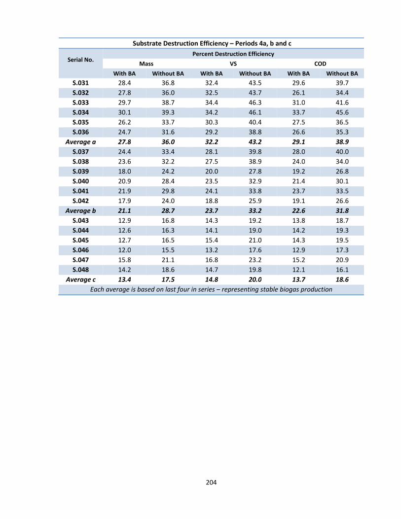
204
Substrate Destruction Efficiency – Periods 4a, b and c
Serial No.
Percent Destruction Efficiency Mass VS COD
With BA Without BA With BA Without BA With BA Without BA S.031 28.4 36.8 32.4 43.5 29.6 39.7 S.032 27.8 36.0 32.5 43.7 26.1 34.4 S.033 29.7 38.7 34.4 46.3 31.0 41.6 S.034 30.1 39.3 34.2 46.1 33.7 45.6 S.035 26.2 33.7 30.3 40.4 27.5 36.5 S.036 24.7 31.6 29.2 38.8 26.6 35.3
Average a 27.8 36.0 32.2 43.2 29.1 38.9 S.037 24.4 33.4 28.1 39.8 28.0 40.0 S.038 23.6 32.2 27.5 38.9 24.0 34.0 S.039 18.0 24.2 20.0 27.8 19.2 26.8 S.040 20.9 28.4 23.5 32.9 21.4 30.1 S.041 21.9 29.8 24.1 33.8 23.7 33.5 S.042 17.9 24.0 18.8 25.9 19.1 26.6
Average b 21.1 28.7 23.7 33.2 22.6 31.8 S.043 12.9 16.8 14.3 19.2 13.8 18.7 S.044 12.6 16.3 14.1 19.0 14.2 19.3 S.045 12.7 16.5 15.4 21.0 14.3 19.5 S.046 12.0 15.5 13.2 17.6 12.9 17.3 S.047 15.8 21.1 16.8 23.2 15.2 20.9 S.048 14.2 18.6 14.7 19.8 12.1 16.1
Average c 13.4 17.5 14.8 20.0 13.7 18.6 Each average is based on last four in series – representing stable biogas production

205
Substrate Destruction Efficiency – Periods 5a, b, c, and d - BA changes
Serial No.
Percent Destruction Efficiency Mass VS COD
With BA Without BA With BA Without BA With BA Without BA S.049 30.2 39.5 32.4 43.5 29.9 40.0 S.050 31.2 40.8 32.0 42.9 30.9 41.4 S.051 32.4 42.5 33.8 45.4 31.0 41.6 S.052 30.4 39.6 31.9 42.8 27.7 36.9 S.053 34.0 44.8 35.5 47.9 35.9 48.8 S.054 35.6 47.0 38.9 52.8 37.0 50.2 S.055 39.5 52.4 43.2 58.9 39.7 54.2 S.056 36.2 47.9 39.0 53.0 39.1 53.4
Average a 36.4 48.0 39.1 53.1 37.9 51.7 S.057 35.3 46.6 37.7 51.1 36.6 49.8 S.058 35.3 46.6 37.6 50.9 32.8 44.3 S.059 31.6 41.3 33.5 45.1 30.7 41.2 S.060 32.5 42.7 34.9 47.0 32.2 43.4 S.061 31.7 41.5 33.9 45.6 35.4 47.9 S.062 32.1 42.1 34.3 46.1 31.8 42.8
Average b 32.0 41.9 34.1 45.9 32.5 43.8 S.063 30.1 39.2 33.0 44.3 29.1 39.0 S.064 32.4 42.5 35.9 48.4 31.0 41.6 S.065 28.2 36.6 31.6 42.4 26.0 34.4 S.066 29.7 38.7 32.8 44.1 30.5 40.9 S.067 36.2 47.9 39.4 53.6 39.1 53.4 S.068 36.9 48.8 40.3 54.8 34.5 46.6
Average c 32.7 43.0 36.1 48.7 32.5 43.9 S.069 31.4 41.1 35.6 48.1 33.4 45.1 S.070 34.3 45.1 39.5 53.6 36.2 49.1 S.071 34.8 45.9 38.9 52.9 37.8 51.4 S.072 38.8 51.4 43.0 58.7 42.1 57.7 S.073 39.2 52.0 43.9 60.0 39.4 53.8
Average d 36.8 48.6 41.3 56.3 38.9 53.0 Each average is based on last four in series – representing stable biogas production

206
Substrate Destruction Efficiency – Period 6a and b -
Serial No.
Percent Destruction Efficiency Mass VS COD
With BA Without BA With BA Without BA With BA Without BA S.074 43.0 56.9 46.9 63.7 43.9 59.6 S.075 42.0 55.4 46.9 63.6 40.4 54.7 S.076 39.1 51.4 45.1 61.1 37.9 51.2 S.077 40.8 53.8 45.7 61.9 41.2 55.8 S.078 42.1 55.6 49.0 66.7 43.0 58.3 S.079 42.4 56.1 47.4 64.4 43.3 58.8
Average a 41.1 54.2 46.8 63.5 41.3 56.0 S.080 49.7 63.7 54.0 71.0 49.9 65.4 S.081 49.0 62.8 53.4 70.1 48.0 62.7 S.082 47.2 60.4 51.7 67.8 51.0 66.8 S.083 47.3 60.5 52.3 68.6 50.6 66.3 S.084 45.5 58.0 49.6 64.9 49.8 65.2 S.085 42.9 54.6 48.2 63.0 47.4 61.9 S.086 45.4 57.9 48.9 63.9 43.3 56.3 S.087 28.0 34.5 33.1 42.1 24.1 29.8
Average b 48.3 61.8 52.9 69.4 49.9 65.3 Average a based on last four in series Average b based on first four in series – see text
Coupon Destruction Data – No. Data Points
Substrate Destruction Efficiency - number of data points
NP 6 6 5 33 6 3
FP 6 6 6 29 6 3
CB 5 6 6 33 6 3
BB 6 5 6 30 6 3
BA 2 2 2 10 2 1
%CODFW 0 7.9 12.9 17.2 21.7 29.3

207
BMP - 2 Substrate Destruction Efficiency
Experiment %CH4 mL. biogas
mL. CH4
COD Destr. mg
COD added mg
COD Destr.% Stdev
CB 56 35.9 20.1 50.6 91.9 55.0 1.5
BB 56 33.9 19.0 47.8 92.5 51.6 0.7
NP 48 9.4 4.5 11.3 96.5 11.7 1.3
FP 45 60.1 27.1 68.1 90.9 74.9 3.6
BA 51 28.0 14.3 36.0 110.0 32.7 2.2
FW 49 58.7 28.8 72.4 110.0 65.8 0.7
FBFW0 45 42.6 19.2 48.2 92.5 52.1 1.3
FBFW6 47 42.5 20.0 50.2 93.3 53.8 0.8
FBFW8 52 44.4 23.1 58.0 93.9 61.8 1.7
FBFW13 46 45.0 20.7 52.1 94.4 55.2 0.8
FBFW17 49 46.6 22.8 57.4 95.0 60.5 2.3
FBFW20 48 44.3 21.2 53.5 95.4 56.0 0.9
FBFW27 48 45.0 21.6 54.3 96.6 56.3 2.4
CBFW 49 47.4 23.2 58.4 93.9 62.2 1.8
BBFW 49 44.2 21.6 54.5 94.5 57.6 1.7
NPFW 32 17.0 5.4 13.7 97.8 14.0 2.7
FPFW 45 62.6 28.2 70.8 93.2 76.0 2.1
BAFW 56 33.6 18.8 47.3 110.0 43.0 2.8

208
Leach Bed Permeability Tests Period 5 – Bulking Agent Assessment
0
100
200
300
400
500
600
0 200 400 600 800 1000 1200 1400 1600 1800 2000
Volu
me
Drai
ned
(ml)
Time (seconds)
LL01 S.061 BA5
LL02 S.062 BA5
LL03 S.063 BA4
LL04 S.058 BA5
LL05 S.059 BA5
LL06 S.060 BA5
2016/06/08 Week 64
0
100
200
300
400
500
600
0 200 400 600 800 1000 1200 1400 1600 1800 2000
Volu
me
Drai
ned
(ml)
Time (seconds)
LL01 S.067 BA4
LL02 S.068 BA4
LL03 S.063 BA4
LL04 S.064 BA4
LL05 S.065 BA4
LL06 S.066 BA4
2016/07/13 Week 69
All LBs contain BA4. Avg substr destr. eff. of these

209
0
100
200
300
400
500
600
0 200 400 600 800 1000 1200 1400 1600 1800 2000
Volu
me
Dra
ined
(ml)
Time (seconds)
LL01 S.073 BA6
LL02 S.074 BA6
LL03 S.075 BA6
LL04 S.070 BA6
LL05 S.071 BA6
LL06 S.072 BA6
2016/08/31 Week 76
0
100
200
300
400
500
600
0 200 400 600 800 1000 1200 1400 1600 1800 2000
Volu
me
Drai
ned
(ml)
Time (seconds)
LL01 S.073 BA6
LL02 S.074 BA6
LL03 S.069 BA6
LL04 S.070 BA6
LL05 S.071 BA6
LL06 S.072 BA6

210
Appendix E – Biogas Data Biogas Production – 88 Week Summary
Biogas Methane Grand Totals As measured At STP At STP Total GM1 GM2 Total GM1 GM2 Total GM1 GM2
Litres 41749 4584 37165 38378 4216 34171 20121 2466 17656
% of Total 100 11 89 100 11 89 100 12.3 87.7
% Methane 52.4 58.5 51.7 52.4 58.5 51.7
Weekly Biogas Production
Biogas Volume - Litres
Biogas Volume - Litres
Methane
As
measured
GM2 temp
. Atm.
Pressure Corrected to STP
Week Total GM1 GM2 °C kPa Total GM1 GM2 Total
1 234.8 72.2 162.6 23.4 1004.9 215.2 66.2 149.0 115.9
2 500.6 245.6 255.0 23.4 999.2 461.5 226.4 235.1 253.7
3 564.2 213.5 350.7 23.4 1003.9 517.6 195.9 321.8 280.7
4 578.0 118.8 459.2 23.4 1005.8 529.3 108.8 420.5 280.8
5 596.7 127.3 469.4 23.4 992.6 553.7 118.1 435.5 294.3
6 500.5 114.8 385.7 23.4 1003.5 459.4 105.4 354.0 245.6
7 519.8 104.5 415.3 23.4 1004.6 476.6 95.8 380.7 252.5
8 513.6 74.5 439.1 23.4 1005.4 470.5 68.3 402.3 247.8
9 491.0 67.0 424.0 23.4 1004.1 450.4 61.5 388.9 237.0
10 526.4 81.0 445.4 23.4 1005.5 482.2 74.2 408.0 254.2
11 481.9 71.3 410.6 23.4 1005.1 441.6 65.3 376.3 232.4
12 498.9 73.3 425.6 23.4 996.1 461.3 67.8 393.6 243.1
13 489.5 80.5 409.0 23.4 999.8 450.9 74.2 376.8 238.0
14 537.7 83.2 454.5 23.4 999.5 495.5 76.7 418.8 261.3
15 505.4 65.0 440.4 23.4 998.9 466.0 59.9 406.1 245.0
16 318.3 23.4 294.7 23.4 1002.0 292.6 21.5 270.9 154.7
17 434.5 48.0 386.5 23.4 996.1 401.8 44.4 357.4 210.8
18 435.6 52.7 382.9 23.4 996.8 402.5 48.7 353.8 211.6
19 452.2 67.6 384.6 23.4 997.4 417.6 62.4 355.2 219.9
20 389.3 57.4 331.9 23.4 999.7 358.7 52.9 305.8 188.9
21 463.9 66.0 397.9 23.4 1001.0 426.9 60.7 366.1 243.1
22 441.4 53.4 388.0 23.4 1000.5 406.3 49.2 357.2 213.3
23 313.0 3.9 309.1 23.4 1002.3 287.6 3.6 284.0 148.9
24 328.6 37.5 291.1 23.4 1002.9 301.8 34.4 267.3 158.4
25 69.9 4.1 65.8 23.4 998.1 64.5 3.8 60.7 33.5
26 463.6 57.2 406.4 23.4 1004.9 424.9 52.4 372.5 223.0
27 542.2 69.9 472.3 23.4 1010.9 494.0 63.7 430.3 259.6

211
28 613.8 72.4 541.4 23.4 1009.6 560.0 66.0 493.9 294.0
29 618.7 75.7 543.0 23.4 999.6 570.1 69.7 500.3 299.1
30 549.5 42.3 507.2 23.4 1000.7 505.8 38.9 466.8 264.7
31 567.4 35.5 531.9 23.4 1007.8 518.5 32.4 486.1 270.2
32 471.0 27.6 443.4 23.4 999.4 434.1 25.4 408.6 225.9
33 415.7 28.2 387.5 23.4 1006.2 380.5 25.8 354.7 198.4
34 409.8 27.7 382.1 23.4 999.7 377.6 25.5 352.0 196.9
35 431.0 32.7 398.3 23.4 1003.6 395.6 30.0 365.6 206.3
36 408.8 26.3 382.5 23.4 1013.2 371.6 23.9 347.7 193.6
37 405.6 22.3 383.3 23.4 1008.0 370.6 20.4 350.2 193.2
38 352.8 19.2 333.6 23.4 997.2 325.9 17.7 308.1 169.5
39 335.4 17.7 317.7 23.4 998.8 309.3 16.3 293.0 161.0
40 296.6 17.8 278.8 23.4 1003.8 272.1 16.3 255.8 142.0
41 282.1 17.3 264.8 23.4 1002.7 259.1 15.9 243.2 135.0
42 290.2 16.0 274.2 23.4 1003.1 266.5 14.7 251.8 138.4
43 279.2 13.7 265.5 23.4 992.8 259.0 12.7 246.3 134.7
44 198.8 2.2 196.6 23.4 1006.8 181.9 2.0 179.9 94.1
45 167.3 4.1 163.2 23.4 993.9 155.0 3.8 151.2 80.3
46 140.5 4.7 135.8 23.4 1001.5 129.2 4.3 124.9 67.1
47 138.9 4.7 134.2 23.4 1002.4 127.6 4.3 123.3 66.4
48 126.3 5.5 120.8 23.4 1002.5 116.0 5.1 111.0 60.3
49 123.7 6.8 116.9 23.4 994.1 114.6 6.3 108.3 59.6
50 279.5 45.9 233.6 23.4 1004.4 256.3 42.1 214.2 135.4
51 347.3 73.1 274.2 23.4 1002.3 319.1 67.2 252.0 169.5
52 387.1 42.8 344.3 23.4 999.0 356.9 39.5 317.4 187.3
53 427.5 37.5 390.0 23.4 999.6 393.9 34.6 359.4 205.9
54 457.9 26.5 431.4 23.4 995.5 423.7 24.5 399.2 220.4
55 479.7 18.3 461.4 23.4 998.3 442.6 16.9 425.7 229.7
56 508.4 18.6 489.8 23.4 1013.6 462.0 16.9 445.1 239.9
57 586.5 19.3 567.1 23.4 1004.4 537.8 17.7 520.0 278.9
58 578.6 16.0 562.6 23.4 1002.3 531.7 14.7 517.0 276.0
59 561.0 17.3 543.7 23.4 995.9 518.8 16.0 502.8 269.1
60 546.9 20.4 526.5 23.4 1000.1 503.6 18.8 484.9 261.2
61 490.9 29.7 461.2 23.4 1004.8 450.0 27.2 422.8 234.4
62 449.1 34.4 414.7 23.4 1001.0 413.2 31.7 381.6 215.4
63 425.1 33.9 391.2 23.4 997.3 392.6 31.3 361.3 204.8
64 425.1 32.6 392.5 23.4 997.0 392.7 30.1 362.6 205.2
65 444.8 39.3 405.5 23.4 1001.6 409.0 36.1 372.9 213.9
66 421.8 36.4 385.4 23.4 1000.3 388.4 33.5 354.9 203.1
67 465.9 30.4 435.5 23.4 1000.7 428.8 28.0 400.8 223.5
68 503.5 36.2 467.3 23.4 996.7 465.3 33.5 431.8 242.8
69 532.6 43.5 489.1 23.4 999.5 490.8 40.1 450.7 256.4
70 495.4 38.2 457.2 23.4 1001.6 455.6 35.1 420.5 237.5

212
71 466.4 35.7 430.7 23.4 1001.0 429.1 32.8 396.3 224.0
72 494.1 40.0 454.1 23.4 1001.0 454.7 36.8 417.9 237.3
73 569.7 41.1 528.6 23.4 1000.6 524.4 37.8 486.6 273.5
74 526.2 51.4 474.8 23.4 999.4 484.9 47.4 437.6 253.7
75 624.5 53.2 571.3 23.4 1005.5 572.1 48.7 523.3 298.9
76 653.0 54.4 598.6 23.4 1006.2 597.8 49.8 548.0 312.4
77 634.7 44.8 589.9 23.4 1000.7 584.2 41.2 543.0 304.6
78 586.7 40.9 545.8 23.4 1004.2 538.1 37.5 500.6 280.5
79 607.3 48.6 558.7 23.4 1005.5 556.3 44.5 511.8 290.4
80 616.3 60.8 555.5 23.4 1004.3 565.2 55.8 509.5 296.1
81 686.7 78.0 608.7 23.4 1009.0 626.9 71.2 555.7 328.7
82 794.1 86.5 707.6 23.4 1005.1 727.7 79.3 648.5 381.1
83 815.7 82.4 733.5 23.4 998.4 752.5 76.0 676.7 394.2
84 786.2 93.5 692.7 23.4 1007.3 718.9 85.5 633.4 376.9
85 783.6 101.5 682.1 23.4 1008.3 715.8 92.7 623.1 376.4
86 798.0 95.1 702.9 23.4 1004.4 731.8 87.2 644.6 384.1
87 802.6 118.4 684.2 23.4 999.7 739.5 109.1 630.4 389.5
88 874.1 113.6 760.5 23.4 1008.4 798.3 103.8 694.6 419.3
Totals 41749 4584 37165 38363 4212 34150 20130

213
Appendix F – Biochemical Methane Potential Tests Contains:
BMP – 1 Synthetic feed procedures BMP – 2 Food waste fibres and bulking agent , Synergy
BMP- 1 testing of synthetic feed and its components Kärt and Nigel
February – March 2015 SOLUTIONS TO BE PREPARED
1. Prepare anaerobic medium according to the protocol „Procedure for preparing basic mineral medium“ with handwritten modifications specified on paper. Store inside the glovebox for a few days until the solution is clear. Pink colour is a sign of oxygen – should not be present! If solution turns pinkish, shake up the FeS and allow to oxidize, if necessary, add FeS.
2. Prepare anaerobic inocculum diluted in medium, incubate a few days at 37°C. A diluted inocculum is easier to pipette. After incubation take a sample for TS+VS measurement and store at 4°C.
3. Prepare (anaerobic) feedstock solutions, measure COD, TS, VS and store frozen or at 4°C. 4. Prepare sterile anaerobic water. First autoclave, then sparge the water with nitrogen, store
inside the glovebox.
THINGS TO BE AUTOCLAVED
1. Autoclave BMP bottles (160 mL), label them and leave open inside the glovebox for a few days. 2. Autoclave rubber stoppers for the bottles, store inside the glovebox. 3. Autoclave a beaker for medium, a graduated cylinder and a small funnel for medium and a beaker
for water, store inside the glovebox.
PREPARATION OF THE GLOVEBAG
In the fumehood of WB303 attach a glovebag to
Gasline on the left Pump on the right (pump is located WB344 next to 105°C oven).
Use a tube and anaerobic tape to attach the end of the tubes to the bag. Use connectors in between! N2 and N2+CO2 are necessary to flush the glovebag.
Put the following things to the glovebag:
Labelled BMP bottles closed with rubber stoppers in a tray (24+extra) A beaker for medium (~500 mL) Graduated cylinder for medium (100 mL) A small funnel for medium A beaker for water (~250 mL) 5 mL pipette 10 mL pipette 5 mL cut tips for inocculum (2+extras)
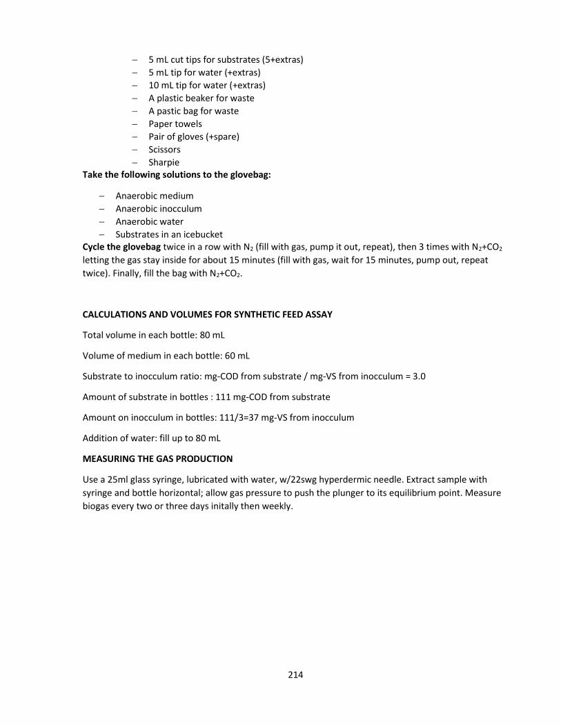
214
5 mL cut tips for substrates (5+extras) 5 mL tip for water (+extras) 10 mL tip for water (+extras) A plastic beaker for waste A pastic bag for waste Paper towels Pair of gloves (+spare) Scissors Sharpie
Take the following solutions to the glovebag:
Anaerobic medium Anaerobic inocculum Anaerobic water Substrates in an icebucket
Cycle the glovebag twice in a row with N2 (fill with gas, pump it out, repeat), then 3 times with N2+CO2 letting the gas stay inside for about 15 minutes (fill with gas, wait for 15 minutes, pump out, repeat twice). Finally, fill the bag with N2+CO2.
CALCULATIONS AND VOLUMES FOR SYNTHETIC FEED ASSAY
Total volume in each bottle: 80 mL
Volume of medium in each bottle: 60 mL
Substrate to inocculum ratio: mg-COD from substrate / mg-VS from inocculum = 3.0
Amount of substrate in bottles : 111 mg-COD from substrate
Amount on inocculum in bottles: 111/3=37 mg-VS from inocculum
Addition of water: fill up to 80 mL
MEASURING THE GAS PRODUCTION
Use a 25ml glass syringe, lubricated with water, w/22swg hyperdermic needle. Extract sample with syringe and bottle horizontal; allow gas pressure to push the plunger to its equilibrium point. Measure biogas every two or three days initally then weekly.

215
# Bottle Medium (mL) Inocculum (mL) Water (mL) Substrate (mL)
1 Tembec negative 60 1.5 18.5 0
2 Tembec negative 60 1.5 18.5 0
3 Tembec negative 60 1.5 18.5 0
4 Tembec + SF 60 1.5 15.47 3.03
5 Tembec + SF 60 1.5 15.47 3.03
6 Tembec + SF 60 1.5 15.47 3.03
7 MF sludge negative 60 2.8 17.2 0
8 MF sludge negative 60 2.8 17.2 0
9 MF sludge negative 60 2.8 17.2 0
10 MF sludge +SF 60 2.8 14.17 3.03
11 MF sludge +SF 60 2.8 14.17 3.03
12 MF sludge +SF 60 2.8 14.17 3.03
13 MF sludge + starch 60 2.8 14.15 3.05
14 MF sludge + starch 60 2.8 14.15 3.05
15 MF sludge + starch 60 2.8 14.15 3.05
16 MF sludge + CMC 60 2.8 13.84 3.36
17 MF sludge + CMC 60 2.8 13.84 3.36
18 MF sludge + CMC 60 2.8 13.84 3.36
19 MF sludge + peptone 60 2.8 14.18 3.02
20 MF sludge + peptone 60 2.8 14.18 3.02
21 MF sludge + peptone 60 2.8 14.18 3.02
22 MF sludge + lipids 60 2.8 14.3 2.9
23 MF sludge + lipids 60 2.8 14.3 2.9
24 MF sludge + lipids 60 2.8 14.3 2.9
Total 1440 59.4 365.4 55.2 Fill the bottles according to the table, close them with rubber stoppers and crimp with metal rings. Store at 37°C, no shaking (WB344).

216
BMP - 2 testing of Food Waste, Fibres and Bulking Agent March - April 2016
5. SOLUTIONS TO BE PREPARED
a. Prepare anaerobic medium according to the protocol - Procedure for preparing basic mineral medium - with handwritten modifications specified on paper. Store inside the glovebox for a few days until the solution is clear. Pink colour is a sign of oxygen – should not be present! If solution turns pinkish, shake up the FeS and allow to oxidize, if necessary, add FeS.
b. Prepare anaerobic inocculum diluted in medium (1:1), incubate a few days at 37°C. A diluted inocculum is easier to pipette. After incubation take a sample for TS+VS measurement and store at 4°C.
c. Prepare (anaerobic) feedstock solution, consisting of centrifuge supernatant of a food waste suspension (3000g for 10 min.) measure COD, TS, VS and store frozen or at 4°C.
d. Prepare sterile anaerobic water. First autoclave, then sparge the water with nitrogen, store inside the glovebox.
6. SUBSTRATES TO BE PREPARED
a. Fibre Samples
Prepare fibre samples (cardboard, boxboard, fine paper and newsprint – individually, and as a blend of all four) as follows: weigh 6.00g (dry weight) of individual substrates (or 11g of mix of four substrates), place in Bendtec blender; add 800ml of DI water; blend 7x, 50 seconds each, (1@ speed 1, 3@ speed 5 and 3@ speed 7); transfer to 1 litre beaker using 200ml of DI water; put on a stir plate and pipette 6x10ml (while stirring) to weighed Al dishes for TS/VS measurements (105oC, 545oC). Pipette 10ml of fibre suspension (while stirring) and dilute to 200ml in a volumetric flask, and perform standard COD measurement. Transfer ~250ml of suspension to each of two deep Al dishes; evaporate to dryness at 105oC (allow 2 days); remove dry sample; cut into narrow strips with scissors; grind strips in a Wiley mill through a 20 mesh screen; preserve sample in a Falcon tube in the fridge.
b. Bulking Agent Sample Prepare BA sample as follows; dry 12g of BA at 105oC overnight; grind in a Wiley mill through a 20 mesh screen; measure TS/VS/COD as for fibre above (suspending 6g of ground BA in water, blending only once at speed 1); preserve balance of sample in a Falcon tube in the fridge.
c. Food Waste Sample - Solid Prepare food waste sample as follows: weigh 250g of sorted FW (remove big bones, pieces of metal, plastic, etc.); place in Blendtec blender; add 250ml of water; blend 4x (1@ speed 1 and 3@ speed 3); transfer ~5g of pulp to each of 3 Al weighing dishes for TS/VS measurements (37oC, 545oC); transfer ~50g of pulp to each of two deep Al dishes; evaporate to dryness at 37oC (allow 3 days); remove dry sample; cut into narrow strips with scissors; grind strips in a Wiley mill through a 20 mesh screen;
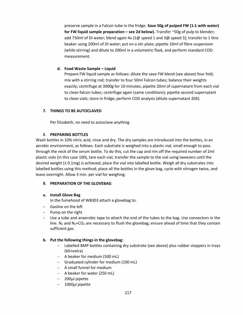
217
preserve sample in a Falcon tube in the fridge. Save 50g of pulped FW (1:1 with water) for FW liquid sample preparation – see 2d below). Transfer ~50g of pulp to blender; add 750ml of DI water; blend again 4x (1@ speed 1 and 3@ speed 3); transfer to 1 litre beaker using 200ml of DI water; put on a stir plate; pipette 10ml of fibre suspension (while stirring) and dilute to 200ml in a volumetric flask, and perform standard COD measurement.
d. Food Waste Sample – Liquid Prepare FW liquid sample as follows: dilute the save FW blend (see above) four fold; mix with a stirring rod; transfer to four 50ml Falcon tubes; balance their weights exactly; centrifuge at 3000g for 10 minutes; pipette 20ml of supernatant from each vial to clean falcon tubes; centrifuge again (same conditions); pipette second supernatant to clean vials; store in fridge; perform COD analysis (dilute supernatant 20X).
7. THINGS TO BE AUTOCLAVED Per Elizabeth, no need to autoclave anything.
8. PREPARING BOTTLES Wash bottles in 10% nitric acid, rinse and dry. The dry samples are introduced into the bottles, in an aerobic environment, as follows. Each substrate is weighed into a plastic vial, small enough to pass through the neck of the serum bottle. To do this, cut the cap and rim off the required number of 2ml plastic vials (in this case 100), tare each vial, transfer the sample to the vial using tweezers until the desired weight (± 0.1mg) is achieved, place the vial into labelled bottle. Weigh all dry substrates into labelled bottles using this method; place all the bottles in the glove bag, cycle with nitrogen twice, and leave overnight. Allow 3 min. per vial for weighing.
9. PREPARATION OF THE GLOVEBAG
a. Install Glove Bag In the fumehood of WB303 attach a glovebag to:
Gasline on the left Pump on the right Use a tube and anaerobic tape to attach the end of the tubes to the bag. Use connectors in the
line. N2 and N2+CO2 are necessary to flush the glovebag; ensure ahead of time that they contain sufficient gas.
b. Put the following things in the glovebag: Labelled BMP bottles containing dry substrate (see above) plus rubber stoppers in trays
(60+extra) A beaker for medium (500 mL) Graduated cylinder for medium (100 mL) A small funnel for medium A beaker for water (250 mL) 200µl pipette 1000µl pipette
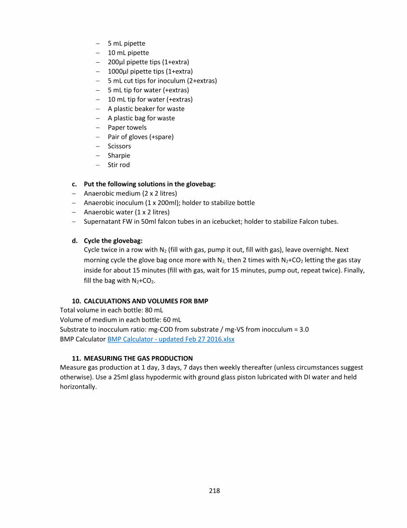
218
5 mL pipette 10 mL pipette 200µl pipette tips (1+extra) 1000µl pipette tips (1+extra) 5 mL cut tips for inoculum (2+extras) 5 mL tip for water (+extras) 10 mL tip for water (+extras) A plastic beaker for waste A plastic bag for waste Paper towels Pair of gloves (+spare) Scissors Sharpie Stir rod
c. Put the following solutions in the glovebag: Anaerobic medium (2 x 2 litres) Anaerobic inoculum (1 x 200ml); holder to stabilize bottle Anaerobic water (1 x 2 litres) Supernatant FW in 50ml falcon tubes in an icebucket; holder to stabilize Falcon tubes.
d. Cycle the glovebag:
Cycle twice in a row with N2 (fill with gas, pump it out, fill with gas), leave overnight. Next morning cycle the glove bag once more with N2, then 2 times with N2+CO2 letting the gas stay inside for about 15 minutes (fill with gas, wait for 15 minutes, pump out, repeat twice). Finally, fill the bag with N2+CO2.
10. CALCULATIONS AND VOLUMES FOR BMP Total volume in each bottle: 80 mL Volume of medium in each bottle: 60 mL Substrate to inocculum ratio: mg-COD from substrate / mg-VS from inocculum = 3.0 BMP Calculator BMP Calculator - updated Feb 27 2016.xlsx
11. MEASURING THE GAS PRODUCTION Measure gas production at 1 day, 3 days, 7 days then weekly thereafter (unless circumstances suggest otherwise). Use a 25ml glass hypodermic with ground glass piston lubricated with DI water and held horizontally.
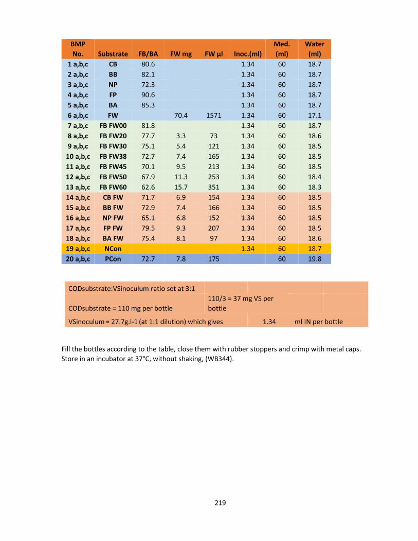
219
BMP No. Substrate FB/BA FW mg FW µl Inoc.(ml)
Med. (ml)
Water (ml)
1 a,b,c CB 80.6 1.34 60 18.7 2 a,b,c BB 82.1 1.34 60 18.7 3 a,b,c NP 72.3 1.34 60 18.7 4 a,b,c FP 90.6 1.34 60 18.7 5 a,b,c BA 85.3 1.34 60 18.7 6 a,b,c FW 70.4 1571 1.34 60 17.1 7 a,b,c FB FW00 81.8 1.34 60 18.7 8 a,b,c FB FW20 77.7 3.3 73 1.34 60 18.6 9 a,b,c FB FW30 75.1 5.4 121 1.34 60 18.5
10 a,b,c FB FW38 72.7 7.4 165 1.34 60 18.5 11 a,b,c FB FW45 70.1 9.5 213 1.34 60 18.5 12 a,b,c FB FW50 67.9 11.3 253 1.34 60 18.4 13 a,b,c FB FW60 62.6 15.7 351 1.34 60 18.3 14 a,b,c CB FW 71.7 6.9 154 1.34 60 18.5 15 a,b,c BB FW 72.9 7.4 166 1.34 60 18.5 16 a,b,c NP FW 65.1 6.8 152 1.34 60 18.5 17 a,b,c FP FW 79.5 9.3 207 1.34 60 18.5 18 a,b,c BA FW 75.4 8.1 97 1.34 60 18.6 19 a,b,c NCon 1.34 60 18.7 20 a,b,c PCon 72.7 7.8 175 60 19.8
CODsubstrate:VSinoculum ratio set at 3:1
CODsubstrate = 110 mg per bottle 110/3 = 37 mg VS per bottle
VSinoculum = 27.7g.l-1 (at 1:1 dilution) which gives 1.34 ml IN per bottle
Fill the bottles according to the table, close them with rubber stoppers and crimp with metal caps. Store in an incubator at 37°C, without shaking, (WB344).

220
Appendix G Financial Projections Contains:
Assumptions 10 year Income statement
Commercial Plant Financial Projections
MODEL ASSUMPTIONS AND OUTPUT
Acquisition Operation
Purchase Price $1,666,667
Organics tipping fee 100.00 $/tonne
Permitting Compost sale revenue - $/tonne
Cover Soil Ratio 0.20 tonne/tonne
Permitting cost $ Cover Soil Cost 5.00 $/tonne
Time to obtain permit
1 years Bulking Agent Ratio 0.25 tonne/tonne
Permitting costs spread uniformly over permitting period Bulking Agent Cost 5.00 $/tonne
Time to construct following permitting
1 years Reject material volume 10% of input
Reject material disposal fee 60.00 $/tonne
Financial Analysis
Drainage/Cover material cost 50,000 $/year
Property taxes 10,000 $/year
Discount Rate 12% Liquor Disposal Cost 0.02 $/litre
Fixed assets depreciated over operating life of site. Condensate Disposal Cost 0.02 $/litre
Tax Rate 35% Diesel Fuel Cost 1.00 $/litre
Host Fee
2.00 $/tonne Equipment O&M Cost = 1.00 x

221
Escalators
Primary reactor residence time 1 years
tipping fee 2% / year Curing time 0.75 years
labour 2% / year Volume Reduction 80% of input
fuel & consumables 2% / year Energy recovered 5.7 MJ/kg
equipment, tires & parts 2% / year Fuel Sales Net Revenue 2.00 $/GJ
other 2% / year Carbon Credit Revenue 5.00 $/GJ
Site Development Decommissioning
Site development spread over 4 years Operating Life 37
Site Decommisioned in year 40
MODEL OUTPUT
NET PRESENT VALUE
$15,086,000
INTERNAL RATE OF RETURN
41%
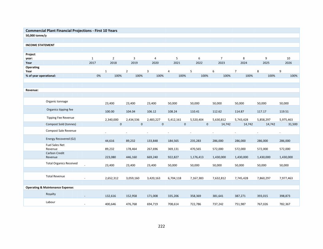
222
Commercial Plant Financial Projections - First 10 Years
50,000 tonne/y
INCOME STATEMENT Project year:
1
2
3
4
5
6
7
8
9
10
Year 2017 2018 2019 2020 2021 2022 2023 2024 2025 2026 Operating Year
1
2
3
4
5
6
7
8
9
% of year operational: 0% 100% 100% 100% 100% 100% 100% 100% 100% 100%
Revenue:
Organic tonnage 23,400
23,400
23,400
50,000
50,000
50,000
50,000
50,000
50,000
Organics tipping fee 100.00
104.04
106.12
108.24
110.41
112.62
114.87
117.17
119.51
Tipping Fee Revenue 2,340,000
2,434,536
2,483,227
5,412,161
5,520,404
5,630,812
5,743,428
5,858,297
5,975,463
Compost Sold (tonnes) 0 0 0 0 0 14,742 14,742 14,742 31,500
Compost Sale Revenue -
-
-
-
-
-
-
-
-
Energy Recovered (GJ) 44,616
89,232
133,848
184,565
235,283
286,000
286,000
286,000
286,000
Fuel Sales Net Revenue
89,232
178,464
267,696
369,131
470,565
572,000
572,000
572,000
572,000
Carbon Credit Revenue
223,080
446,160
669,240
922,827
1,176,413
1,430,000
1,430,000
1,430,000
1,430,000
Total Organics Received -
23,400
23,400
23,400
50,000
50,000
50,000
50,000
50,000
50,000
Total Revenue -
2,652,312
3,059,160
3,420,163
6,704,118
7,167,383
7,632,812
7,745,428
7,860,297
7,977,463
Operating & Maintenance Expense:
Royalty -
132,616
152,958
171,008
335,206
358,369
381,641
387,271
393,015
398,873
Labour -
400,646
476,768
694,719
708,614
722,786
737,242
751,987
767,026
782,367

223
Fuel / Oil / Filters/Tires/Parts
-
-
-
-
-
-
-
-
-
-
Leased Equipment
-
25,500
26,010
26,530
27,061
27,602
28,154
28,717
29,291
29,877
Cover Soil 23,868
24,345
24,832
54,122
55,204
56,308
57,434
58,583
59,755
Bulking Agent
29,835
-
-
-
-
-
-
-
-
Road Building Materials
-
9,180
9,364
9,551
9,742
9,937
10,135
10,338
10,545
10,756
Drainage/Cover Materials
-
51,000
52,020
53,060
54,122
55,204
56,308
57,434
58,583
59,755
Reject material disposal
-
-
-
-
155,013
158,113
161,275
351,498
358,528
Liquor Disposal 90,698
185,025
283,088
494,412
615,900
742,051
873,001
890,461
908,270
Condensate Disposal
4,774
9,738
14,899
26,022
32,416
39,055
45,947
46,866
47,804
Insurance -
26,523
30,592
34,202
67,041
71,674
76,328
77,454
78,603
79,775
Environmental Management
-
22,236
22,681
23,134
23,597
24,069
24,550
25,041
25,542
26,053
Office Expense -
42,840
43,697
44,571
45,462
46,371
47,299
48,245
49,210
50,194
Utilities -
35,027
35,727
36,442
37,171
37,914
38,672
39,446
40,235
41,039
Property Tax
-
10,200
10,404
10,612
10,824
11,041
11,262
11,487
11,717
11,951
Host Fee -
47,736
48,691
49,665
108,243
110,408
112,616
114,869
117,166
119,509
Total O & M Expense
-
952,678
1,128,019
1,476,313
2,001,637
2,333,908
2,519,735
2,689,947
2,928,341
2,984,505
Site Decommissioning
-
-
-
-
-
-
-
-
-
-
EBITDA -
1,699,634
1,931,141
1,943,849
4,702,481
4,833,474
5,113,077
5,055,481
4,931,956
4,992,958
% of Revenue
64.08% 63.13% 56.83% 70.14% 67.44% 66.99% 65.27% 62.75% 62.59%
Revenue ($/tonne) 113.35
130.73
146.16
134.08
143.35
152.66
154.91
157.21
159.55
Operating Cost ($/tonne) -
40.71
48.21
63.09
40.03
46.68
50.39
53.80
58.57
59.69

224
Depreciation
256,179
342,193
520,969
631,558
760,579
915,404
1,128,177
1,386,219
1,773,281
Debt Service
Interest
Amortization
Total Debt Service
DSCR
EBIT 1,443,455
1,588,948
1,422,880
4,070,923
4,072,896
4,197,673
3,927,304
3,545,737
3,219,676
Interest -
EBT 1,443,455
Tax 505,209
Net Income 938,246
Related Documents