The Algebraic Reconstruction Technique of Lambert-Beer's attenuation approximation for parallel rays transmission projection

2011 International Conference on Electrical Engineering and Informatics 17-19 July 2011, Bandung, Indonesia

The Algebraic Reconstruction Technique of Lambert-Beer’s Attenuation Approximation for

Parallel Rays Transmission Projection M. Amin #1, D. Sudiana*2, D. Gunawan#3

# Department of Electrical Engineering, Faculty of Engineering, Universitas Indonesia, Kampus Baru UI Depok, West Java, Indonesia

[email protected] [email protected]

*Computer Engineering Study Program, Department of Electrical Engineering Faculty of Engineering, Universitas Indonesia, Kampus UI Depok, West Java, Indonesia

[email protected]

Abstract— The Algebraic Reconstruction Technique (ART) of Lambert-Beer’s attenuation approximation for parallel rays transmission projection is a variant of the ART model that aims to solve image reconstruction problems in nuclear based computed tomography for non-destructive testing where γ or x radiation is used as a ray source . In this model, the path length of the ray that hits a pixel at any projection view and the size of detector grid are explicitly included in computation. Then, the model is used to investigate the influence of the ray path length and the width of detector grid in producing image quality. The image quality is represented as space and pixel resolution, respectively. In this paper, we demonstrate that the model is able to show the contribution of the ray path length and detector grid in producing image quality. By considering ray path length and detector grid, the model produces smaller Root Mean Square error compared to conventional ART. Keywords— nuclear computed tomography, image quality, ray path length, detector grid, ART, Lambert Beer’s attenuation law.

I. INTRODUCTION

Nuclear based computed tomography is imaging technique that uses nuclear radiation such as γ or x-ray as a ray source. Not only in medical treatments, nuclear based computed tomography is also applied for non-destructive testing. In nuclear based tomography, an image of cross sectional object under investigation is obtained by placing the object between parallel detector grids and γ or x-ray source system. The system is moved around the object to get parallel projection data from several views. The data are then reconstructed using a tomography algorithm to produce tomography image.

The idea of tomography has been launched since 1950s. Since then, a number of algorithms have been proposed for doing reconstruction. Each of which has some gains and shortcomings. Algebraic reconstruction technique (ART) is one of them.

ART is time and memory consuming when involving a large number of projections, however, ART has ability to reconstruct an object with limited projection views [1]-[2].

With this ability, ART is mainly proposed in reconstructing a larger object.

ART is a recursive calculation method to estimate the attenuation coefficients of an interior object from some projection views. The interior object is assumed as a set of unknown cross sections. To estimate the value of cross sections, a number of parallel projection data at different views must be previously provided. The data are gained by passing a penetrative ray in a certain quantity such as γ or x-ray through a side of an object. Then, the unabsorbed quantity of the penetrative ray that comes out from another side of the object is measured and compared to the initial quantity. This method is called transmission method. The recursive calculation will be end if it satisfies a stopping criterion.

ART that has many variants generally used to solve a linear set of equation [1]-[6], [13] as represented in Eq. 1. μ ∑ μ , 1,2, … , (1)

where p represents one dimensional vector. The vector contains N elements, which each element has a known value. N is the multiplication between the number of projections and the number of rays or detector parallel grids. The detector that has as many as possible grids is assumed to be equal or larger than the object dimension. A ray or a detector grid represents the pixel width. pi is the value of p at row i. µ is one dimensional scalar containing as much as I square of pixel rows. Each row has one pixel of unknown value. I square represents the dimension of image. µj is the value of µ at row j. W is a weight matrix and wij is the coefficient of the weight matrix. It scores 1 if any ray passes through a pixel and 0 otherwise. Eq. 1 shows that projection value at row i (pi) is obtained from the sum of multiplication between weight coefficient (wij) at row i and column j and pixel value (µj) at row j of image matrix that has been transformed to one dimensional scalar matrix.

H4 - 2

978-1-4577-0752-0/11/$26.00 ©2011 IEEE

In many papers on tomography, ART is proposed to reconstruct image of quality from limited projection views. A number of ART corrections were proposed to decrease errors in order to improve image quality [6]-[12].

Image quality can be measured from its resolution, namely the ability of image to recognize the smallest data as a pixel and to represent the object under investigation as a number of pixels. For this case, the image quality consists of two resolutions: image pixel resolution and image space resolution, respectively. Accordingly, the higher the value to represent pixel image the higher the pixel resolution is and the smaller the size of pixel thickness the higher the space resolution is. Therefore, for the same object, the pixel resolution of gray level of 65536 is higher than that of 256, the space resolution image of size 1024 1024 is better than that of 512 512.

Surely, image resolution in nuclear based computed tomography for non-destructive testing is influenced by the width of detector grid, detector sensitivity of γ or x-rays, and assumptions of the ART models in processing the pixel values. The width of detector grid represents the size of the pixel, while the detector sensitivity is the ability of detector to transform any incoming γ or x-ray to digital data. The length of ray path that passes through a pixel, and the ability of ART to reconstruct the data as a pixel of image, contributes to the pixel resolution.

Unfortunately, papers in nuclear based computed tomography using ART have not demonstrated explicitly the contribution of a ray path length and the width of detector grid in producing image. Accordingly, in this paper we investigated the contribution of the length of ray path and the width of detector grid explicitly in producing pixel image using ART of Lambert-Beer’s attenuation approximation by simulation.

The next section starts discussing the characteristic of γ or x-ray transmission with regard to Lambert-Beer’s attenuation law.

II. LAMBERT-BEER’S ATTENUATION LAW

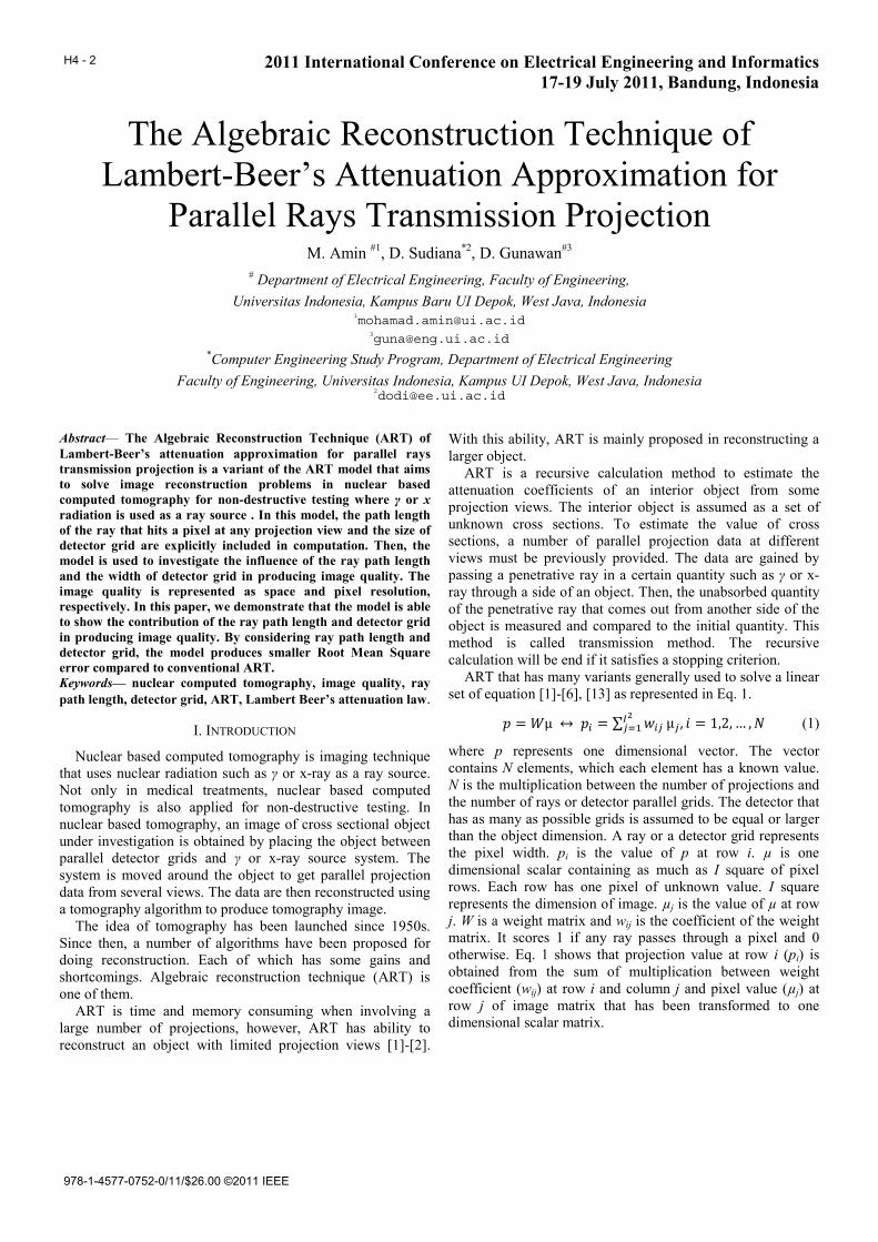
If γ or x-ray as a vector of certain energy and intensity passes through an object of homogenous composition, then its intensity will be attenuated by the object following the Lambert-Beer’s attenuation law. Let I0 is the initial intensity before passing the object, µ is the object attenuation coefficient and dx is the ray path in x direction in the object as shown in Fig. 1, then the intensity of the ray I after passing the object satisfies the Lambert-Beer attenuation law [2][5] as expressed in Eq. 2.

Fig. 1. The γ or x-ray intensity before (I0) and after (I ) passing an object of thickness dx and attenuation coefficient µ according to Lambert-Beer’s law

2

A negative sign in Eq. 2 shows that initial intensity I0 of a ray will drop to intensity I exponentially when the ray penetrates an object.

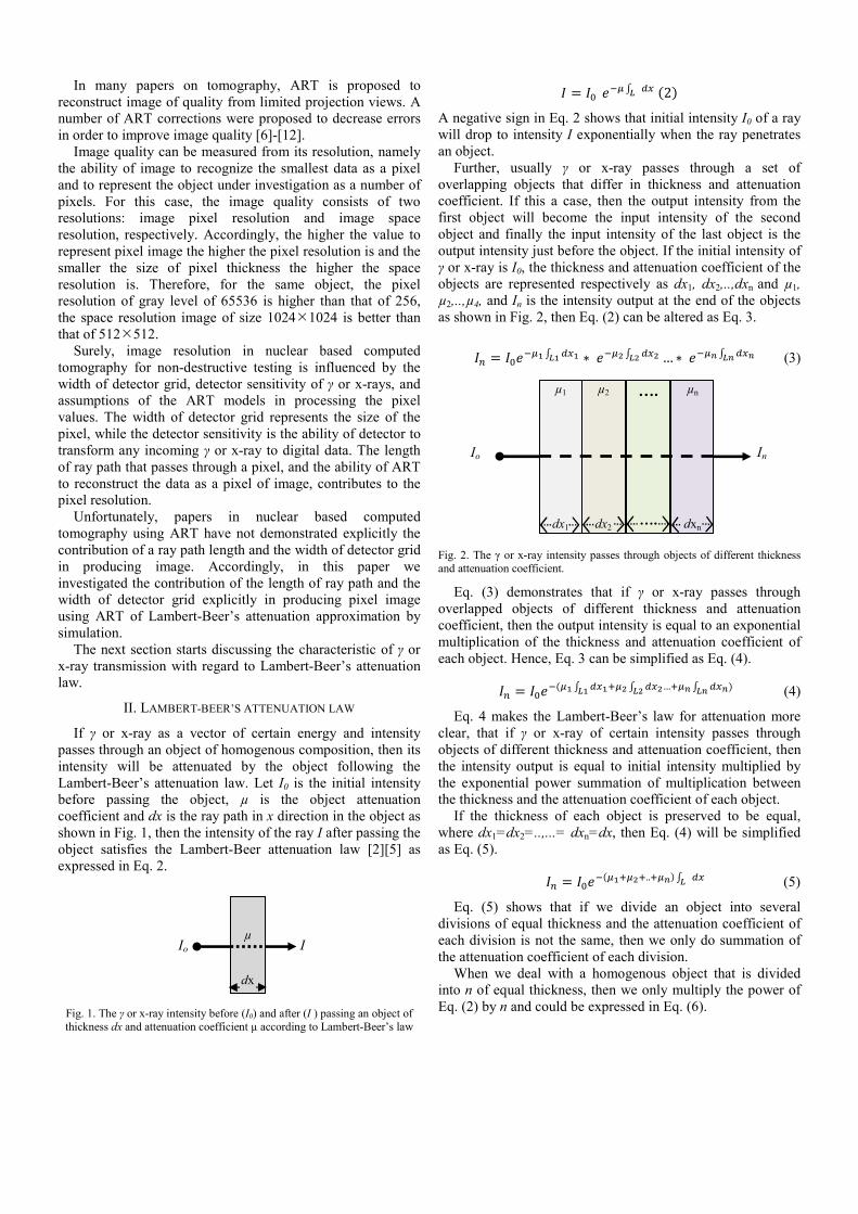
Further, usually γ or x-ray passes through a set of overlapping objects that differ in thickness and attenuation coefficient. If this a case, then the output intensity from the first object will become the input intensity of the second object and finally the input intensity of the last object is the output intensity just before the object. If the initial intensity of γ or x-ray is I0, the thickness and attenuation coefficient of the objects are represented respectively as dx1, dx2,..,dxn and µ1, µ2,..,µ4, and In is the intensity output at the end of the objects as shown in Fig. 2, then Eq. (2) can be altered as Eq. 3.

… (3)

Fig. 2. The γ or x-ray intensity passes through objects of different thickness and attenuation coefficient.

Eq. (3) demonstrates that if γ or x-ray passes through overlapped objects of different thickness and attenuation coefficient, then the output intensity is equal to an exponential multiplication of the thickness and attenuation coefficient of each object. Hence, Eq. 3 can be simplified as Eq. (4). … (4)

Eq. 4 makes the Lambert-Beer’s law for attenuation more clear, that if γ or x-ray of certain intensity passes through objects of different thickness and attenuation coefficient, then the intensity output is equal to initial intensity multiplied by the exponential power summation of multiplication between the thickness and the attenuation coefficient of each object.

If the thickness of each object is preserved to be equal, where dx1=dx2=..,...= dxn=dx, then Eq. (4) will be simplified as Eq. (5). .. (5)

Eq. (5) shows that if we divide an object into several divisions of equal thickness and the attenuation coefficient of each division is not the same, then we only do summation of the attenuation coefficient of each division.

When we deal with a homogenous object that is divided into n of equal thickness, then we only multiply the power of Eq. (2) by n and could be expressed in Eq. (6).

Io I I

µ

dx

Io In

µ1

dx1

µ2

dx2

µn

dxn

….

….

(6)

Because the multiplication between n and the thickness of each division (dx) is equal to the width of the homogenous object, then Eq. (6) means that the output intensity of a γ or x-ray after passing through a homogenous object will decrease by following the multiplication between the intensity of the ray before penetrating the object and the exponential multiplication between the attenuation coefficient and the thickness of the object.

III. LINEAR FORM OF LAMBERT BEER’S ATTENUATION

In order to get a simple computation relationship between intensity and attenuation coefficient at a given distance, then Lambert-Beer’s attenuation must be changed to a linear form. In general, with refer to Eq. (2) and by assuming the length of ray path that penetrating a an object is x, then the Lambert-Beer’s attenuation can be changed into a linear form as shown in Eq. (7).

(7) Eq. (7) reveals that the natural logarithm of comparison

between output and input intensity is proportionally depends on the attenuation coefficient multiplied the distance of ray path in a homogenous object. As a result, the linear Lambert-Beer’s attenuation in Eq. (4)-(6) are represented respectively in the following Eqs. (8)-(10). (8)

(9)

(10)

Eq. (8) shows that the comparison of output to input intensity is equal to the summation of multiplication between the thickness and the attenuation coefficient of each material that compose an object. In case the thickness of each material is arranged to equal, then Eq. (8) could be expressed as Eq. (9). Further, if the object is a homogeneous composition then it follows Eq. (10), where x is the length and the direction of γ or x-ray which is parallel to the x-axis.

IV. DETECTOR GRID AND Γ OR X-RAY PATH CONTRIBUTION

In a digital image, a pixel is represented by a point or small circle where the pixel perimeter (length) is assumed to be 1. In the nuclear based tomography for non-destructive testing, however, a pixel is basically retrieved either from the ability of a detector to make a step movement, or from the size of detector grid if it is an array detector. The size of detector grid is commonly used to represent the size of pixel. Therefore, a pixel is modeled as a square of grid.

The size of detector grid determines the number of pixels that represent an image. This can be explained by referring to Fig. 3. The figure shows that there are 9 detectors of equal grids used to receive parallel rays that passing through an object. Therefore, there are 81 of pixels representing the

image. If the grid of the array detector is changed to a smaller one, then the number of pixels will increase. Consequently, smaller size of grid resulted in increasing number of pixels. Similarly, the greater the number of pixels we use, the better the image quality will be.

The mathematical relationship to determine the number of pixels can be obtained from the number of segments, which are obtained if the size of detector grid and the object length are previously known. Let g is the width of detector grid, o is the length of the object, then the number of segments s are given by Eq. (11). / (11)

Eq. (11) demonstrates that the number of segments that can

be used to display an object image, are equal to the length of the object divided by the size of detector grid.

Fig. 3. The number of segments that can be detected by detector is equal to the number of detector grid.

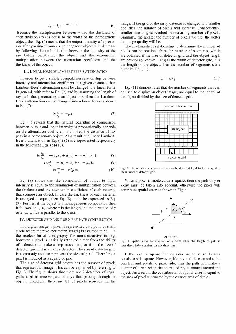
When a pixel is modeled as a square, then the path of γ or

x-ray must be taken into account, otherwise the pixel will contribute spatial error as shown in Fig. 4.

Fig. 4. Spatial error contribution of a pixel when the length of path is considered to be constant for any direction.

If the pixel is square then its sides are equal, so its area equals to side square. However, if a ray path is assumed to be constant and equals to pixel side, then the path will make a quarter of circle when the source of ray is rotated around the object. As a result, the contribution of spatial error is equal to the area of pixel subtracted by the quarter area of circle.

Δl =x =y=1

θ y Δl

x

γ ray pencil bar source

a detector grid

an object

Let Δl is the length of ray path, y is the length of pixel in vertical direction, x is the length of pixel in horizontal direction. Then, if Δl=x=y=1, the spatial error contribution of the ray path (ersp) is given by Eq. (12). ∆ 1 1 16⁄ (12)

The spatial error contribution of pixel can be removed whenever the path length of ray from any direction is inserted into calculation as illustrated in Fig. 5. In this case the pixel area is a function of ray path that rotated smoothly from horizontal to vertical direction by summing its vertical projection length and its horizontal projection length. The vertical and horizontal projection lengths are absolute. Finally, the length of γ or x-ray Δl that passes through a square section in the object under investigation is a function of direction and represented as formulated in Eq. (13). ∆ | . | | . | (13)

Usually y=x=g because it represents the size of detector grid (g). Therefore, Eq. (13) can be simplified as Eq. (14). ∆ | | | | (14)

Fig. 5. Removing pixel spatial error by considering the contribution of ray path direction

It seems clear that the detector grid and γ or x-ray path has

a main contribution in the determination of image quality.

V. ART OF LAMBERT-BEER’S ATTENUATION

ART of Lambert-Beer’s attenuation adopts the algebraic reconstruction technique proposed firstly by Kaczmarz in order to be practically used to solve Eq. (1) in nuclear based computed tomography for non-destructive testing. Kaczmarz ART is also called additive ART and has been further developed to improve its performance, such as Brook ART, Mayinger ART, Gordon ART, Gilbert ART, Anderson [1]-[5], [7]. Generally, ART of Lambert-Beer’s attenuation is as shown in Eq. (15). ∑∑ (15) where, is the updated attenuation coefficient, is the current attenuation coefficient. i represents a pixel position in an object image which is ordered sequentially from 1 at the top left to I square at the bottom right of the image dimension. is a relaxation parameter, is weight matrix used to separate between the attenuation coefficient and the

length of ray path at row i column j. also represents the contribution of detector grid width in the image. is the total attenuation coefficient projection at row i, is the current attenuation coefficient used to make correction between and the calculated total attenuation coefficient. , 0 ,

is the detector grid width, while is the projection angle at row i.

VI. SIMULATION SETUP

To show the contribution of a ray path length and the width of detector grid at a pixel and a space resolution by simulation then we did two main steps as follows:

A. Preparation Steps

a. Eqs. (1) and (15) were compiled into MATLAB source code. The source code of Eq. (1) was used to generate data as if the data were from projections ( ). The source code of Eq. (15) was used to make reconstruction from projection data generated by Eq. (1). With regard to Eq. (15), we made a bit modification of simultaneous ART of Anderson [2] in order that the ART is able to be used as ART of Lambert-Beer’s attenuation.

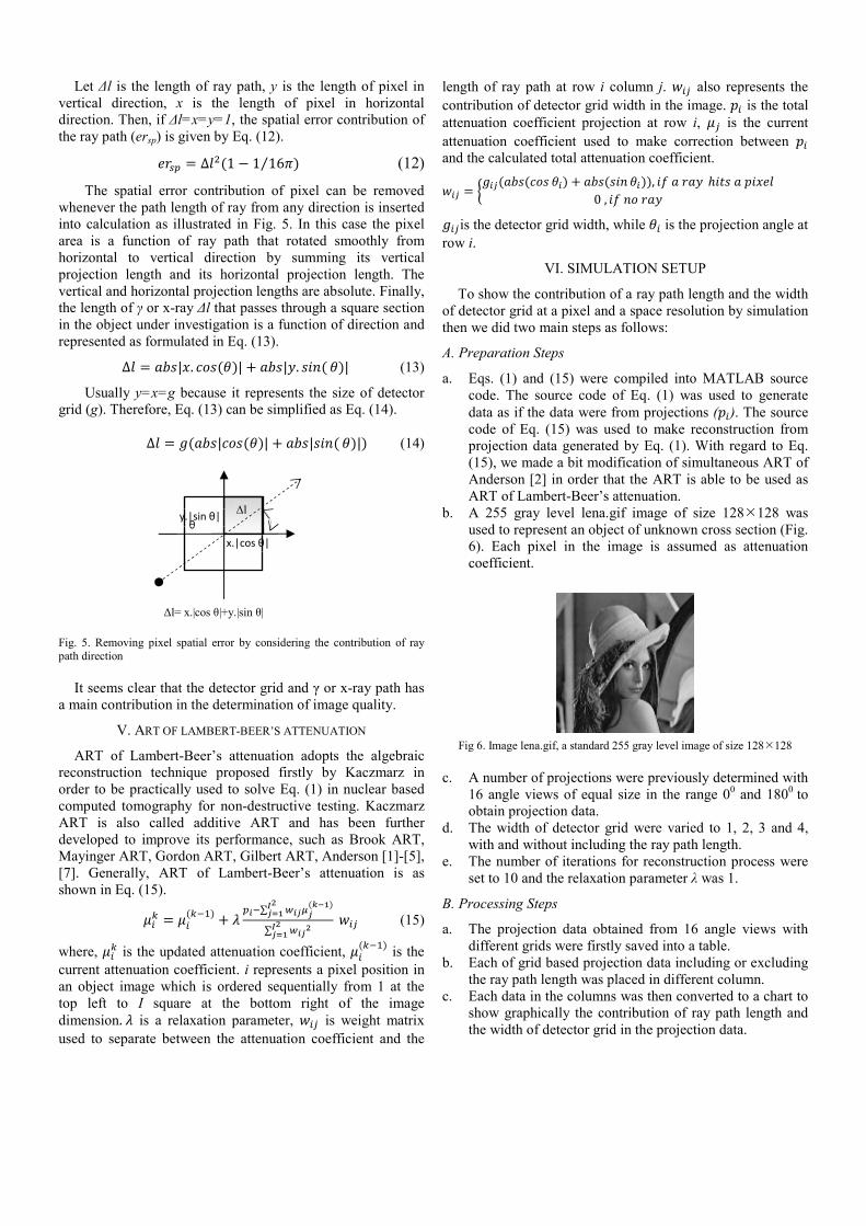
b. A 255 gray level lena.gif image of size 128 128 was used to represent an object of unknown cross section (Fig. 6). Each pixel in the image is assumed as attenuation coefficient.

Fig 6. Image lena.gif, a standard 255 gray level image of size 128 128 c. A number of projections were previously determined with

16 angle views of equal size in the range 00 and 1800 to obtain projection data.

d. The width of detector grid were varied to 1, 2, 3 and 4, with and without including the ray path length.

e. The number of iterations for reconstruction process were set to 10 and the relaxation parameter λ was 1.

B. Processing Steps

a. The projection data obtained from 16 angle views with different grids were firstly saved into a table.

b. Each of grid based projection data including or excluding the ray path length was placed in different column.

c. Each data in the columns was then converted to a chart to show graphically the contribution of ray path length and the width of detector grid in the projection data.

Δl= x.|cos θ|+y.|sin θ|

Δl θ

x.|cos θ|

y.|sin θ|

d. The projection data were then processed using the Matlab source code of Eq. (15) to obtain a reconstruction image of each grid by including or excluding the ray path length.

e. The reconstruction images were used to compare the pixel resolution and space resolution between the grids including or excluding the ray path length visually.

f. The reconstruction image of grid one was used to compare the RMS error contribution between image that included the influence of ray path length and that did not.

VII. RESULTS AND DISCUSSION

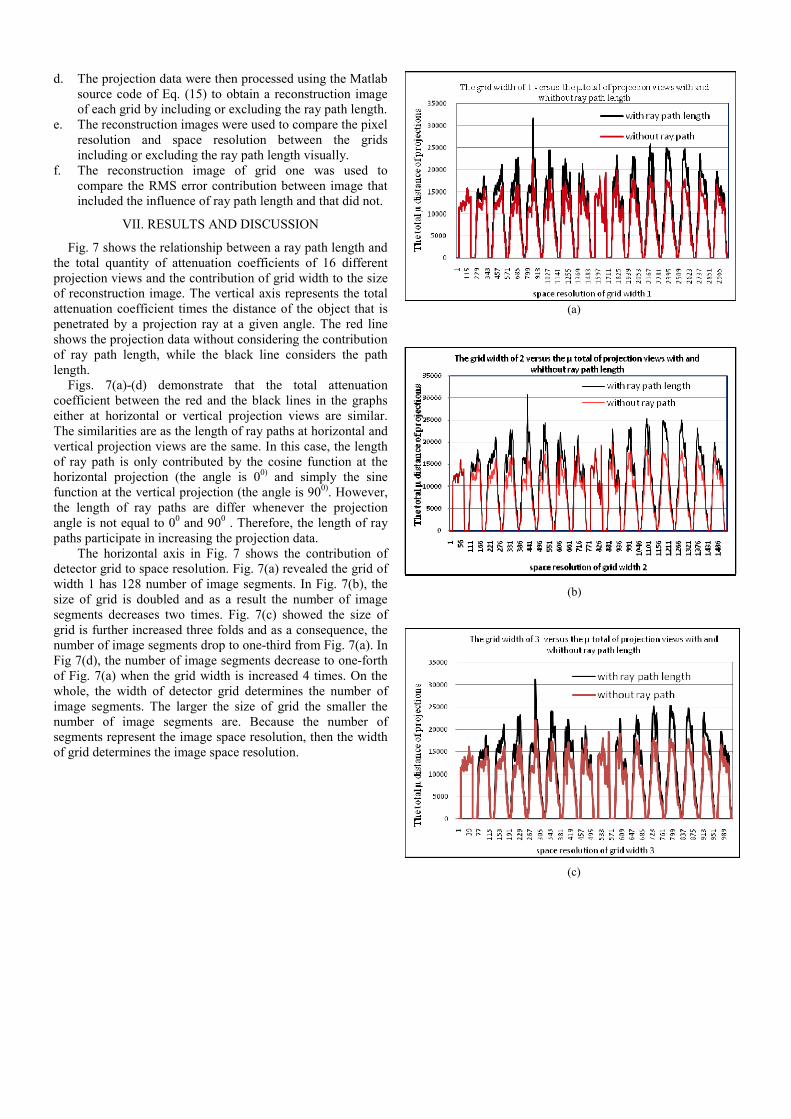
Fig. 7 shows the relationship between a ray path length and the total quantity of attenuation coefficients of 16 different projection views and the contribution of grid width to the size of reconstruction image. The vertical axis represents the total attenuation coefficient times the distance of the object that is penetrated by a projection ray at a given angle. The red line shows the projection data without considering the contribution of ray path length, while the black line considers the path length.

Figs. 7(a)-(d) demonstrate that the total attenuation coefficient between the red and the black lines in the graphs either at horizontal or vertical projection views are similar. The similarities are as the length of ray paths at horizontal and vertical projection views are the same. In this case, the length of ray path is only contributed by the cosine function at the horizontal projection (the angle is 00) and simply the sine function at the vertical projection (the angle is 900). However, the length of ray paths are differ whenever the projection angle is not equal to 00 and 900 . Therefore, the length of ray paths participate in increasing the projection data.

The horizontal axis in Fig. 7 shows the contribution of detector grid to space resolution. Fig. 7(a) revealed the grid of width 1 has 128 number of image segments. In Fig. 7(b), the size of grid is doubled and as a result the number of image segments decreases two times. Fig. 7(c) showed the size of grid is further increased three folds and as a consequence, the number of image segments drop to one-third from Fig. 7(a). In Fig 7(d), the number of image segments decrease to one-forth of Fig. 7(a) when the grid width is increased 4 times. On the whole, the width of detector grid determines the number of image segments. The larger the size of grid the smaller the number of image segments are. Because the number of segments represent the image space resolution, then the width of grid determines the image space resolution.

(c)

(b)

(a)

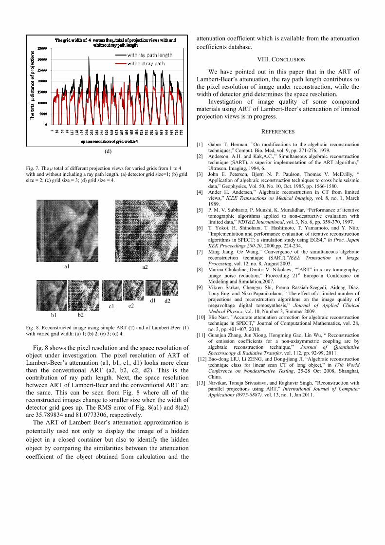
Fig. 7. The μ total of different projection views for varied grids from 1 to 4 with and without including a ray path length. (a) detector grid size=1; (b) grid size = 2; (c) grid size = 3; (d) grid size = 4.

Fig. 8. Reconstructed image using simple ART (2) and of Lambert-Beer (1) with varied grid width: (a) 1; (b) 2; (c) 3; (d) 4.

Fig. 8 shows the pixel resolution and the space resolution of

object under investigation. The pixel resolution of ART of Lambert-Beer’s attenuation (a1, b1, c1, d1) looks more clear than the conventional ART (a2, b2, c2, d2). This is the contribution of ray path length. Next, the space resolution between ART of Lambert-Beer and the conventional ART are the same. This can be seen from Fig. 8 where all of the reconstructed images change to smaller size when the width of detector grid goes up. The RMS error of Fig. 8(a1) and 8(a2) are 35.789834 and 81.0773306, respectively.

The ART of Lambert Beer’s attenuation approximation is potentially used not only to display the image of a hidden object in a closed container but also to identify the hidden object by comparing the similarities between the attenuation coefficient of the object obtained from calculation and the

attenuation coefficient which is available from the attenuation coefficients database.

VIII. CONCLUSION

We have pointed out in this paper that in the ART of Lambert-Beer’s attenuation, the ray path length contributes to the pixel resolution of image under reconstruction, while the width of detector grid determines the space resolution.

Investigation of image quality of some compound materials using ART of Lambert-Beer’s attenuation of limited projection views is in progress.

REFERENCES

[1] Gabor T. Herman, ”On modifications to the algebraic reconstruction techniques,” Comput. Bio. Med, vol. 9, pp. 271-276, 1979.

[2] Anderson, A.H. and Kak,A.C.,” Simultaneous algebraic reconstruction technique (SART), a superior implementation of the ART algorithm,” Ultrason. Imaging, 1984, 6.

[3] John E. Peterson, Bjorn N. P. Paulson, Thomas V. McEvilly, “ Application of algebraic reconstruction techniques to cross hole seismic data,” Geophysics, Vol. 50, No. 10, Oct. 1985, pp. 1566-1580.

[4] Ander H. Andersen,” Algebraic reconstruction in CT from limited views,” IEEE Transactions on Medical Imaging, vol. 8, no. 1, March 1989.

[5] P. M. V. Subbarao, P. Munshi, K. Muralidhar, “Performance of iterative tomographic algorithms applied to non-destructive evaluation with limited data,” NDT&E International, vol. 3, No. 6, pp. 359-370, 1997.

[6] T. Yokoi, H. Shinohara, T. Hashimoto, T. Yamamoto, and Y. Niio, ”Implementation and performance evaluation of iterative reconstruction algorithms in SPECT: a simulation study using EGS4,” in Proc. Japan KEK Proceedings 200-20, 2000,pp. 224-234.

[7] Ming Jiang, Ge Wang,” Convergence of the simultaneous algebraic reconstruction technique (SART),”IEEE Transaction on Image Processing, vol. 12, no. 8, August 2003.

[8] Marina Chukalina, Dmitri V. Nikolaev, “”ART” in x-ray tomography: image noise reduction,” Proceeding 21st European Conference on Modeling and Simulation,2007.

[9] Vikren Sarkar, Chengyu Shi, Prema Rassiah-Szegedi, Aidnag Diaz, Tony Eng, and Niko Papanikolaou, ” The effect of a limited number of projections and reconstruction algorithms on the image quality of megavoltage digital tomosynthesis,” Journal of Applied Clinical Medical Physics, vol. 10, Number 3, Summer 2009.

[10] Elie Nasr, ”Accurate attenuation correction for algebraic reconstruction technique in SPECT,” Journal of Computational Mathematics, vol. 28, no. 3, pp. 401-407, 2010.

[11] Guanjun Zhang, Jun Xiong, Hongming Gao, Lin Wu, “ Reconstruction of emission coefficients for a non-axisymmetric coupling arc by algebraic reconstruction technique,” Journal of Quantitative Spectroscopy & Radiative Transfer, vol. 112, pp. 92-99, 2011.

[12] Bao-dong LIU, Li ZENG, and Dong-jiang JI, “Algebraic reconstruction technique class for linear scan CT of long object,” in 17th World Conference on Nondestructive Testing, 25-28 Oct 2008, Shanghai, China.

[13] Nirvikar, Tanuja Srivastava, and Raghuvir Singh, ”Reconstruction with parallel projections using ART,” International Journal of Computer Applications (0975-8887), vol. 13, no. 1, Jan 2011.

(d)

a1 a2

b1

d1 d2

b2 c2 c1