Western Kentucky University TopSCHOLAR® Honors College Capstone Experience/esis Projects Honors College at WKU Spring 5-2012 e Ages and Metallicities of Type Ia Supernova Host Galaxies from the Nearby Galaxies Supernova Search Program Suzanna Sadler Western Kentucky University, [email protected] Follow this and additional works at: hp://digitalcommons.wku.edu/stu_hon_theses Part of the Stars, Interstellar Medium and the Galaxy Commons , and the e Sun and the Solar System Commons is esis is brought to you for free and open access by TopSCHOLAR®. It has been accepted for inclusion in Honors College Capstone Experience/ esis Projects by an authorized administrator of TopSCHOLAR®. For more information, please contact [email protected]. Recommended Citation Sadler, Suzanna, "e Ages and Metallicities of Type Ia Supernova Host Galaxies from the Nearby Galaxies Supernova Search Program" (2012). Honors College Capstone Experience/esis Projects. Paper 356. hp://digitalcommons.wku.edu/stu_hon_theses/356

Welcome message from author
This document is posted to help you gain knowledge. Please leave a comment to let me know what you think about it! Share it to your friends and learn new things together.
Transcript

Western Kentucky UniversityTopSCHOLAR®Honors College Capstone Experience/ThesisProjects Honors College at WKU
Spring 5-2012
The Ages and Metallicities of Type Ia SupernovaHost Galaxies from the Nearby GalaxiesSupernova Search ProgramSuzanna SadlerWestern Kentucky University, [email protected]
Follow this and additional works at: http://digitalcommons.wku.edu/stu_hon_theses
Part of the Stars, Interstellar Medium and the Galaxy Commons, and the The Sun and the SolarSystem Commons
This Thesis is brought to you for free and open access by TopSCHOLAR®. It has been accepted for inclusion in Honors College Capstone Experience/Thesis Projects by an authorized administrator of TopSCHOLAR®. For more information, please contact [email protected].
Recommended CitationSadler, Suzanna, "The Ages and Metallicities of Type Ia Supernova Host Galaxies from the Nearby Galaxies Supernova SearchProgram" (2012). Honors College Capstone Experience/Thesis Projects. Paper 356.http://digitalcommons.wku.edu/stu_hon_theses/356

THE AGES AND METALLICITIES OF TYPE IA SUPERNOVA HOST GALAXIES
FROM THE NEARBY GALAXIES SUPERNOVA SEARCH PROGRAM
A Capstone Experience/Thesis Project
Presented in Partial Fulfillment of the Requirements for
the Degree Bachelor of Science with
Honors College Graduate Distinction at Western Kentucky University
By
Suzanna M. Sadler
* * * * *
Western Kentucky University2012
CE/T Committee: Approved by
Dr. Louis-Gregory Strolger
Dr. Michael CariniAdvisor
Dr. Walter Collett Department of Physics & Astronomy

Copyright bySuzanna Marie Sadler
2012

ABSTRACT
We seek to better understand the physical constraints under which White Dwarf stars
ultimately become Type Ia supernovae (SNe Ia), an important test of the robustness of these
tools in precisely measuring Dark Energy, as the definite progenitor system still remains
elusive. The host galaxy environments of Type Ia supernovae provide our best opportunity
for constraining the mechanism(s) of SN Ia production, i.e., the stars involved and the in-
cubation times (tied to stellar ages), and the sensitivity of SNe Ia to changes in the local
metallicity. We have measured the ages and metallicities of approximately 60 galaxies from
a sample of Type Ia supernova hosts collected by the Nearby Galaxies Supernova Search
project. In this manuscript, I present the completed analysis on 16 of these host galax-
ies, comparing their optical spectral data to synthesized galaxy models (from single stellar
populations) to determine the dominant stellar ages and metallicities. Evidence shows a
stronger dependence on the age of the host than the host’s metallicity, apparently conflict-
ing with some predictions. These results are puzzling, but preliminary. A full analysis on
all host data, and perhaps with more complex models, will provide a validity test of the
mostly indirect trends established in other low-z surveys (e.g. Sloan Digital Sky Survey),
and may ultimately steer future investigations for more precise SN Ia cosmology.
Keywords: Astrophysics, Dark Energy, Supernovae, Galaxies, Stellar Populations
ii

Kurt,It’s only the beginning, love.
Dad,What is it like seeing the stars from up there?
Mom,There is nowhere I can go where your prayer has not already been.
Katherine,Thank you for teaching me to never look down on a sister except to pick her up.
Victoria,If life was a cookie, you would definitely be the chocolate chips.
iii

ACKNOWLEDGEMENTS
This work would not have been possible without the exceptional support from count-
less people. I must thank my advisor, Dr. Louis Strolger for all of the time, effort, patience,
dedication, and forgiveness that it took to get me to this point. I also wish to thank the De-
partment of Physics & Astronomy as a whole for their effort in giving students exceptional
support, mentorship, and opportunities. I would also like to acknowledge the numerous
people who contributed to my project in various, though indispensable ways: Schuyler
Wolff, Andrew Gott, and April Pease, along with all of the by-capture proofreaders. There
were countless contributions to this work in other ways that I’ll never know. Thank you all.
Additional acknowledgments to Western Kentucky University’s Ogden College and
Honors College for financial support throughout my career. Funding for my project also
came from a scholarship through the Kentucky Space Grant Consortium.
iv

VITA
May 20, 1991 . . . . . . . . . . . . . . . . . . . . . . . . . . . . . Born - Murray, Kentucky2009 . . . . . . . . . . . . . . . . . . . . . . . . . . . . . . . . . . Carol M. Gatton Academy
of Mathematics and Science,Bowling Green, Kentucky
2009 . . . . . . . . . . . . . . . . . . . . . . . . . . . . . . . . . Trigg County High School,Cadiz, Kentucky
2010 . . . . . . . . . . . . . . . . . . . . . . . . . . . . . . . Pi Mu Epsilon (ΠME) inductee2010 . . . . . . . . . . . . . . . . . . . . . . . . . . . . Department of Physics and Astronomy
Rookie of the Year Award2010 - 2011 . . . . . . . . . . . . . . . . . . . . . . . . . Kentucky Space Grant Consortium
Undergraduate Scholar2011 . . . . . . . . . . . . . . . . . . . . . . . . . . . Randall Harper Award for Outstanding
Research in Physics and Astronomy2011 . . . . . . . . . . . . . . . . . . . . . . . . . . . . . . . Sigma Pi Sigma (ΣΠΣ) inductee2011 - 2012 . . . . . . . . . . . . . . . . . . . . . . . President, Society of Physics Students,
WKU chapter2012 . . . . . . . . . . . . . . . . . . . . . . . . . . . . . Dr. George V. and Sadie Skiles Page
Award for Excellence in Scholarship,Physics and Astronomy
PUBLICATIONS
1. Sadler, S. M., Strolger, L., & Wolff, S. 2011, Bulletin of the American Astronomical Society,43, #337.14
2. Sadler, S. M., Strolger, L., Wolff, S., & Gott, A. 2011, National Conference on UndergraduateResearch, Ithaca College, Ithaca, NY
3. Strolger, L.-G., van Dyk, S., Wolff, S., Campbell, L., Sadler, S. M., & Pease, A. 2011, NOAOProposal ID #2011A-0416, 416
4. Wolff, S., Strolger, L.-G., & Sadler, S. M. 2011, National Conference on Undergraduate Re-search, Ithaca College, Ithaca, NY
5. Sadler, S. M., Strolger, L., Wolff, & S. 2010, Southeastern Section of the American PhysicalSociety, Louisiana State University, Baton Rouge, LA
FIELDS OF STUDY
Major Field: PhysicsMinor Field: Astronomy, Mathematics
v

TABLE OF CONTENTS
ABSTRACT . . . . . . . . . . . . . . . . . . . . . . . . . . . . . . . . . . . . . . . . . ii
ACKNOWLEDGEMENTS . . . . . . . . . . . . . . . . . . . . . . . . . . . . . . . . iv
LIST OF FIGURES . . . . . . . . . . . . . . . . . . . . . . . . . . . . . . . . . . . . vii
LIST OF TABLES . . . . . . . . . . . . . . . . . . . . . . . . . . . . . . . . . . . . . ix
CHAPTER
I. Background and Introduction . . . . . . . . . . . . . . . . . . . . . . . . . . . 1
1.1 Supernovae: An Introduction . . . . . . . . . . . . . . . . . . . . . . . . 21.2 Why Study Supernovae? . . . . . . . . . . . . . . . . . . . . . . . . . . . 41.3 Delay-Time Distribution of Type Ia Supernovae: An Issue of Metallicity or
Age? . . . . . . . . . . . . . . . . . . . . . . . . . . . . . . . . . . . . . 61.4 The Delay Time Distributions . . . . . . . . . . . . . . . . . . . . . . . . 9
II. Data: Groundwork to Present . . . . . . . . . . . . . . . . . . . . . . . . . . . 12
2.1 Groundwork: The Nearby Galaxies Supernova Search Project . . . . . . . 122.2 Host Galaxy Spectra: Kitt Peak & Palomar . . . . . . . . . . . . . . . . . 14
III. Tests of Environmental Effects . . . . . . . . . . . . . . . . . . . . . . . . . . . 17
3.1 Determination of Metallicity and Ages in the Sample . . . . . . . . . . . 173.1.1 The MILES Templates . . . . . . . . . . . . . . . . . . . . . . 193.1.2 The Inadequacies of EZ Ages . . . . . . . . . . . . . . . . . . 193.1.3 The CC-Test . . . . . . . . . . . . . . . . . . . . . . . . . . . 21
IV. Conclusions . . . . . . . . . . . . . . . . . . . . . . . . . . . . . . . . . . . . . 26
4.1 Results & Discussion . . . . . . . . . . . . . . . . . . . . . . . . . . . . 264.1.1 Table of Ages and Metallicities . . . . . . . . . . . . . . . . . 284.1.2 Future Work . . . . . . . . . . . . . . . . . . . . . . . . . . . 28
BIBLIOGRAPHY . . . . . . . . . . . . . . . . . . . . . . . . . . . . . . . . . . . . . 32
vi

LIST OF FIGURES
Figure
1.1 From Filippenko 1997, examples of spectral differences between types of super-novae. . . . . . . . . . . . . . . . . . . . . . . . . . . . . . . . . . . . . . . . . 3
1.2 H-R diagram of stars in the Solar neighborhood, from the Hipparcos catalog (greypoints, Perryman et al. 1997). Red lines indicate isochrones, or lines of stars ofthe same stellar age (annotated on diagram). Stars spend nearly 90% of theirlifetimes on the Main Sequence, in the large group of stars that extend from upperleft to lower right of the diagram. From there they begin a quick death processthat pauses in the Red Giant phase (grouping in the upper right), and for manyculminates as supernovae. The age describes the isochrone, and the mass is theturnoff point of the particular isochrone. . . . . . . . . . . . . . . . . . . . . . . 7
2.1 Sky coverage for the Nearby Galaxies Supernova Search. Each box indicates asingle pointing of the 0.9m + Mosaic (∼ 1 square degree) and are color coded byepoch, or visit. Gray is the template, blue is the second epoch, red is the thirdepoch, and purple is the fourth epoch. . . . . . . . . . . . . . . . . . . . . . . . 13
3.1 Spectrum of host galaxy of SN 1999av. This spectrum shows strong absorptionfeatures – Lick Indices – which passively tell about the chemical enrichment andages of stars in the galaxy. . . . . . . . . . . . . . . . . . . . . . . . . . . . . . 18
3.2 Plot of errors calculated between input parameters and parameters measured byEZ Ages. Colors are based on error percentages of the greatest error (either ageor metallicitiy, indicated in each box). Green boxes indicate errors below 20%,yellow boxes indicate errors between 20% and 50%. Red boxes are 100% errors,or failures. These are combinations that EZ Ages could not output a measure ofage or metallicity. . . . . . . . . . . . . . . . . . . . . . . . . . . . . . . . . . . 20
3.3 Illustration of the Minimum-χ2 fit method between data and a MILES templatespectrum. This plot shows a model that poorly fits the data, shown by its largerresiduals in χ space. . . . . . . . . . . . . . . . . . . . . . . . . . . . . . . . . . 22
vii

3.4 Illustration of the Minimum-χ2 fit method between data and a MILES templatespectrum. This plot shows a model that is a better fit to the data. The residuals inthis comparison are much smaller than Figure 3.3. . . . . . . . . . . . . . . . . . 23
3.5 Illustration of the Minimum-χ2 fit method between data and a MILES templatespectrum. This plot shows a model that returned to be the minimum-χ2 for thedata for SN 1999ep. The residuals in χ space are the smallest out of every possiblecombination. . . . . . . . . . . . . . . . . . . . . . . . . . . . . . . . . . . . . 24
3.6 Contour plot, showing contour regions. The age and metallicity ranges were de-termined by analyzing the darkest region. The white region shows the untestedregion due to lack of MILES spectra. . . . . . . . . . . . . . . . . . . . . . . . . 25
4.1 Final plot with an estimation of Meng’s prediction region overlaid. Upper leftof the plot would include young, star-forming galaxies. Upper right of the plotwould include old, star-forming galaxies. Bottom left of the plot would be unusualgalaxies – young, but lacking in the metal content that one would expect with theincreased metal abundances in the universe (Note that this region was generallyuntestable due to the lack of MILES spectra). Bottom right of the plot wouldcontain old, dying red galaxies that did not undergo many phases of star-formation. 27
viii

LIST OF TABLES
Table
2.1 NGSS Supernovae and revisit-discovered supernovae used in Age/Metallicity com-parison. . . . . . . . . . . . . . . . . . . . . . . . . . . . . . . . . . . . . . . . 16
4.1 Numerical findings from Age/Metallicity comparison. . . . . . . . . . . . . . . . 28
ix

CHAPTER I
Background and Introduction
Dark energy is a pervasive, repulsive force that makes up about 75% of the energy in
the universe. The idea of Dark Energy has roots in the work of Albert Einstein and Edwin
Hubble and proof of its existence has culminated in a Nobel Prize in Physics. The discovery
of Dark Energy leaves in its wake a puzzle, a problem, and a scandal.
The Dark Energy Puzzle: Dark Energy exists! What is the nature of this energy that
seems to dominate the universe?
The Probing Problem: Type Ia supernovae are the best tools to measure the nature of
Dark Energy, but we don’t know why these tools work (i.e. the physics behind their
mechanisms).
The Progression Scandal: Type Ia supernovae may be a diverse set of events, with a
diverse set of progenitor mechanisms, which would cast doubt on our ability to use
them uniformly to measure the nature of Dark Energy. And, so, we are back to square
one.
We must better understand Type Ia supernovae to be confident in our measurements of
the nature of Dark Energy. This requires probing the environments of these events to better
1

constrain the physical mechanisms behind their production.
1.1 Supernovae: An Introduction
Supernovae (SNe) are the catastrophic deaths of certain stars as they explode and ex-
pel mass and energy into space. On average, these events occur once every 100 to 500
years in typical galaxies like our Milky Way (Wolff 2010) and last on the order of a few
months to a year. All supernova events can be placed in one of two physical categories –
thermonuclear or kinematic – based on their differences in basic mechanisms. However,
they are categorized based on characteristics in their optical spectra (See Figure 1.1). In
summary, Type I SNe are distinguished from Type II SNe by their absence of Hydrogen
lines. Within the category of Type I supernovae are three subcategories – Ia (with promi-
nent silicon features), Ib (with prominent helium features), and Ic (with neither helium nor
silicon features).
Types Ib, Ic and Type II events all have similar kinematic origins. These “core-collapse”
events are the result of massive stars that have used up the fuel within their cores, leaving
only iron, which has the highest binding energy per nucleon of any element. At that point,
there is insufficient radiation pressure to support the gravitational pressure, and the star col-
lapses. The collapse is abruptly halted by newly formed neutron degenerate Fe-core, and a
shockwave forms as rebounding material propagates back through the in-falling material.
Neutrinos are produced in the prompt nuclear burning event that explosively expels matter
into space. The core-collapse event mechanism is supported by detailed numerical model-
ing, and recent deep archival imaging from Hubble Space Telescope have routinely shown
the massive (> 8 M) stellar progenitors of these events prior to explosion. (Van Dyk, S.
2

Figure 1.1: From Filippenko 1997, examples of spectral differences between types of supernovae.
D., Li, W., & Filippenko, A. V. 2003)
By contrast, Type Ia supernovae (SNe Ia) are not as well understood as the core-collapse
events, partly because their progenitors have never been observed prior to explosion. It is
generally accepted that SNe Ia are thermonuclear events stemming from C+O White Dwarf
(WD) stars, the remnant of intermediate mass (∼ 3−8 M) stars that have completed the
normal life cycle and have ceased nuclear fusion. In this scenario White Dwarfs are capable
of further highly exothermic fusion reactions if their temperatures rise high enough to burn
carbon and oxygen to Fe-peak elements. This is believed to be achieved through a process
of mass accretion from a neighboring star, and culminates once the WD’s mass exceeds the
1.4 M Chandresekhar Mass Limit. Based on Jean’s mass and Fragmentation arguments,
3

it is generally held that the companion star is roughly the same in zero-age main sequence
mass as the primary, just a little delayed in evolution. Therefore, the companion is thought
to be a Red Giant.
As the progenitor star mass limit is fixed, they all have a fixed maximum intrinsic bright-
ness of MB ∼= -19.5±0.2, corresponding to total energy outputs of around 1×1044 Watts.
(In one second, this event would power the entire world for roughly 1023 years!). The con-
sistency of luminosity makes these events excellent standard candles and excellent probes
of vast cosmic distances via the inverse square law, as shown in Equation 1.1.
(1.1) dL =
√L
4πF
where L is the intrinsic luminosity and F is the absorption-free peak flux observed for the
event. In cosmological terms, this is:
(1.2) dL =(1+ z)
H0
∫ z1
0
1√(1+ z)2(1+ΩMz)− z(2+ z)ΩΛ
dz
where the dL is sensitive to the density of matter (ΩM) and the density of dark energy (ΩΛ)
in a Euclidean (flat) universe where z is the redshift and H0 is the Hubble Constant. As
other astrophysical information tells the density of ordinary and dark matter in the universe,
standard candle distances of SNe Ia provide excellent probes of Dark Energy.
1.2 Why Study Supernovae?
Type Ia supernovae have proven to be excellent standardizable candles, accurate to
within 7% for measuring the expansion history of the universe (Phillips 1993) and us-
ing Equation 1.2, astronomers have uncovered a large Dark Energy component (Riess et
4

al. 1998). However, there is great uncertainty on the details of the physical mechanism by
which White Dwarfs turn into SNe Ia, much of which hinges on the type of mass-donor
stars involved (or more specifically, their ages), and the rate of mass accretion (governed by
the chemical composition of the White Dwarf [Pinto & Eastman 2000; Timmes et al. 2003;
Meng et al. 2011]). The Delay-Time Distribution, or incubation time from stellar birth
to supernova event, was thought to be a way to help resolve the uncertainty in possible
progenitor systems. However, Maoz et al. (2011), Sullivan et al. (2006), and Strolger et
al. (2010) found largely inconsistent results. Further discussion on Delay-Time can be
found in Section 1.3.
The crux of the “scandal” is the uncertainty in Type Ia Supernovae as a Dark Energy
measuring tool. Investigators have found that there are numerous ways to make a SN
Ia from a WD, and perhaps nature utilizes them all, but the amazing uniformity of these
events is perplexing. The “canonical” model (White Dwarf + Red Giant) has an implied
dependence on metallicity. Models suggest (Timmes et al. 2008) metal rich progenitors
will be less luminous SNe Ia, perhaps in a way which invalidates the SN Ia standardization.
What is worse, due to stellar evolution, metal abundances decrease substantially with look-
back time, making SNe Ia now inherently different from SNe Ia in the distant past. It will
necessarily make it tough to measure the strength or evolution in Dark Energy.
Other models (Strolger et al. 2010; Meng et al. 2011) suggest a much less massive,
longer-lived companion, like a Sub-Giant or Main Sequence star. These models infer a
progenitor that is less susceptible to local metallicity variations as this is “locked in” at
very early epochs of the universe. Here, SNe Ia at z ∼ 0.1 are no different from SNe Ia
at z ∼ 1.0, and thus their standard candle distances can be used to probe Dark Energy
accurately and robustly. It is, therefore, extremely important to determine which is the
5

actual mechanism (or companion) White Dwarfs use to make SNe Ia.
Environments, specifically the ages of stars and the metallicity of stars and gas, provide
some constraint on the properties of White Dwarf systems, and can be inferred from galaxy-
global properties such as morphological type, luminosity, and color (Hamuy et al. 2000;
Gallagher et al. 2008; Howell et al. 2009), but thus far the results have been inconclusive.
However, these properties can be more accurately measured in a more direct, albeit time-
consuming, method of spectroscopic measurement and matching to galaxy models, through
indices of ions or molecules, or full spectrum cross-correlation. I have conducted a census
of environments for a sample of low-redshift host galaxies taken from the NGSS, matching
to Vazdekis MILES SSP models via cross-correlation and least-square fits, to constrain the
ages and metallicities of hosts in our sample.
1.3 Delay-Time Distribution of Type Ia Supernovae: An Issue of Metallicity or Age?
It is generally agreed that the progenitor star of SNe Ia is a carbon-oxygen White Dwarf.
However, there is no clear observation that indicates how the extra mass gets close enough
to the White Dwarf for it to incorporate into the star and ignite carbon burning. The question
now lies with the progenitor system; is it singly degenerate or doubly degenerate? That is,
does the White Dwarf accrete mass from a binary companion (Main Sequence or Red Giant
star), or do two White Dwarf stars merge?
One way to test the progenitor systems of these events is to investigate the Delay-Time
Distribution (DTD). The “delay-time” is the time elapsed between a given star’s birth and
its supernova event, and the DTD tells us about the range of progenitor system though
well-established relationships basic basic stellar quantities. Figure 1.2 is the Hertzsprung-
6

Russell (HR) Diagram, a plot depicting the relationships between luminosity, surface tem-
perature, and mass of stars. There are a few fundamental relationships that we can deter-
mine from this diagram.
Figure 1.2: H-R diagram of stars in the Solar neighborhood, from the Hipparcos catalog (greypoints, Perryman et al. 1997). Red lines indicate isochrones, or lines of stars of thesame stellar age (annotated on diagram). Stars spend nearly 90% of their lifetimes onthe Main Sequence, in the large group of stars that extend from upper left to lower rightof the diagram. From there they begin a quick death process that pauses in the Red Giantphase (grouping in the upper right), and for many culminates as supernovae. The agedescribes the isochrone, and the mass is the turnoff point of the particular isochrone.
First, stars occupying the “Main Sequence,” the group of stars extending from the upper
left to lower right of the HR Diagram (Figure 1.2), are all in hydrostatic equilibrium and
are constantly nuclear burning hydrogen into helium in their cores. More massive Main
7

Sequence stars burn through their fuel more rapidly, but they also have more fuel to burn.
Through hydrostatic equilibrium equations, one can derive the relationship between stellar
mass and luminosity for stars on the main sequence, which is:
(1.3) L ∝ M3.5
This equation shows that even a slight change in stellar mass can dramatically affect
the luminosity. Massive stars have greater gravitational compression in their cores due
to the sheer weight of the overlying layers; it follows that low-mass stars have a lower
gravitational compression in their cores. The massive stars, therefore, need greater thermal
and radiation pressure pushing outward to balance the greater gravitational compression
to put the star into hydrostatic equilibrium. The greater thermal pressure is provided by
the higher temperatures in the massive star’s core. Simply put, more massive stars need
higher core temperatures to be stable. Equation 3.1 can be written in terms of the mass and
luminosity of our Sun as follows:
(1.4)L
L=
(M
M
)3.5
where L and M denote the luminosity and mass of our Sun, respectively.
This relation also gives an estimate of the lifetimes of stars of different masses. The
luminosity directly tells how quickly a given star consumes its mass. In a given time (t) it
will then consume a certain amount of its hydrogen fuel (M).
(1.5) L× t = M
8

As this rate of consumption is proportional to the amount of fuel (Equations 1.3 and
1.4), we can estimate the time it would take to consume all of its fuel by substituting into
Equation 1.5
(1.6) M3.5t ∝ M
and simplification yields the relationship between time and mass:
(1.7) t ∝ M−2.5
Equation 1.7 tells us that as the mass of the progenitor star increases, the time it takes
to go through the H-burning phase of its life, the Main Sequence lifetime, decreases nearly
quadratically. Granted, stars do not consume all of their H mass in the H-burning phase,
but they surprisingly eat about the same proportion of their total mass (∼10%) making the
proportionality valid for all Main Sequence stars. More over, the main sequence lifetime of
a star accounts for the vast majority of the total stellar lifetime (∼ 80% - 90% of the total
time from birth to death). Therefore, it is a remarkably suitable to approximation of the
longevity of stars, as illustrated in Figure 1.2.
1.4 The Delay Time Distributions
In single-degenerate SN Ia progenitor systems, the Main Sequence lifetime of the com-
panion stars largely dictate the Delay Time of the events. Simply, the White Dwarf must
wait until its companion has evolved to a point where it can donate material to the White
Dwarf. This criterion is generally met when the companion leaves the Main Sequence H-
burning stage. At this point, the star expands as it moves toward the Red Giant phase, and
9

its surface gravity is greatly reduced, allowing for mass transfer. By contrast, in double-
degenerate systems, the Delay Time is governed by the angular momentum of the WD+WD
pair, the initial separation, and the time necessary to gravitationally radiate away the angu-
lar momentum to “spin up” to collision.
In principle, each system (WD+MS, WD+RG, WD+WD) would have an inherent dis-
tribution of Delay Times, based either on the allowable zero-age Main Sequence mass
ranges of MS or RG companions, or the angular momentum and separation distributions
of WD+WD pairs. A plausible means for determining the Delay Time Distribution (and,
thus, the progenitor system) would be to compare the rate of SNe Ia events in a sample of
galaxies to the rate of star formation in those galaxies.
Work on DTD has yielded mixed results. In the low-redshift regime, Maoz et al. (2011)
showed a short delay time. In the medium range redshift regime, Sullivan et al. (2006)
showed mixed delay times, but dominantly short delays. Strolger et al. (2010) showed that,
in the high-redshift regime, the events preferred a longer delay time. Strolger suggested
that one possible explanation of his results was a minimum metallicity – the universe had
to achieve a certain metal content before the supernova events were possible. Physically,
this means that potential White Dwarf progenitor stars need a level of metallicity to support
an ultraviolet wind that allows steady mass accretion. This wind prevents rapid accretion
that would trigger hydrogen and helium flashes on the surface, causing a nova, and also
prevents accretion-triggered core-collapse supernova (Strolger et al. 2010; Kobayashi &
Nomoto 2009).
Meng et al. (2011) decided to test this possible explanation for the mixed delay times
seen in all redshift regimes. Their attempts at modeling the DTD mark the first attempts to
merge all redshift observations into one explanation. Meng showed that as the metallicity
10

of the progenitor star increased, the mass of the companion star needed to increase. As
determined previously in this section, as the mass of a star increases, the lifetime of the star
decreases. Thus, it is proposed that metal rich progenitor stars (as mostly seen in the low-z
universe) should produce SNe from young populations and the metal poor progenitors in
the high-z universe should be highly delayed.
This provides a testable hypothesis, as the low-z universe, although dominated by metal-
rich systems, includes a substantial population of metal poor systems as well. The test
would be to see if metal rich systems are more prone to producing SNe Ia (by virtue of
having both prompt and delated SNe Ia) than currently metal poor systems which should
only have delayed events. This could be very different from an “age effect” where young
systems that are not necessarily metal rich (e.g. galaxy mergers) may produce more events
than old systems that aren’t necessarily metal poor (e.g. early red ellipticals).
I attempt to show which characteristic (age or metallicity) is most representative of SN
Ia hosts, either demonstrating the Meng et al. (2011) interpretation of metallicity dependent
progenitors or validating one of the DTD interpretations of SN Ia production mechanisms.
11
CHAPTER II
Data: Groundwork to Present
2.1 Groundwork: The Nearby Galaxies Supernova Search Project
The Nearby Galaxies Supernova Search (NGSS) was designed to detect and study low-
redshift supernovae of all types. This survey collected data from 1999 to 2001 using the
0.9-meter telescope and 8k × 8k Mosaic North camera at Kitt Peak National Observatory
(KPNO) just outside of Tucson, Arizona. The campaign consisted of four epochs as shown
in Figure 2.1, surveying nearly 500 square degrees along the celestial equator and out of
the galactic plane. At its time of completion, the Nearby Galaxies Supernova Search was
the largest campaign for low-z supernovae.
In real time, NGSS discovered 42 supernovae, 30 of which were Type Ia. Beginning
in 2005, the data was revisited by Gatton and WKU students using different temporal ca-
dences between template and search-epoch images. This additional searching turned up
an additional 29 potential Type Ia supernovae, bringing our total sample to 59 supernovae
(Wolff 2011; Strolger 2003). Figure 2.1 shows the field coverage for NGSS. The square in
the figure is roughly the size of the constellation Orion, approximately 50 square degrees,
for comparison to the survey. The dotted lines are the outline of the galactic plane; one can
12

easily see that the plane was appropriately avoided in the survey.
60°S
30°S
0°
30°N
60°N
60°S
30°S
0°
30°N
60°N
0 60 120 300 240
Orion
Figure 2.1: Sky coverage for the Nearby Galaxies Supernova Search. Each box indicates a singlepointing of the 0.9m + Mosaic (∼ 1 square degree) and are color coded by epoch, orvisit. Gray is the template, blue is the second epoch, red is the third epoch, and purpleis the fourth epoch.
13

2.2 Host Galaxy Spectra: Kitt Peak & Palomar
The sample of supernovae (and their hosts) collected from the NGSS project provides
an excellent sample for investigating host galaxy environments, as nearly all are bright
enough to adequately illuminate an optical spectrograph on a 4m class telescope within
reasonable integration times.
Along with Schuyler Wolff, Dr. Louis-Gregory Strolger and I applied for and received
four continuous semesters of observing time at the Mayall 4-meter telescope (with the
Ritchey-Chretien Spectrograph) at Kitt Peak National Observatory, and the Hale 5.1-meter
telescope (with the Double Spectrograph) at the Caltech/Palomar Observatory. Over this
campaign, averaging 6 nights per semester, we obtained optical spectra of nearly all 59 of
our SNe Ia and SN Ia candidates.
The setup for each observing run was nearly identical, and optimized to get excellent
signal-to-noise (S/N > 40) at all wavelengths for the full spectral range (3500A - 7500A).
At the Mayall telescope, we used the BL 181 grating (316 l/mm), alternating in first and
second order, with the GG 455 and CuSO4 blocking filters to optimize the red (5000A -
7500A) and blue (3000A - 5500A) spectral responses, respectively. At the Hale telescope,
we could use two spectrograph setups simultaneously, and used the 316 l/mm and 300 l/mm
gratings with no blocking filters.
Both observatories provided high S/N spectra (S/N ≥ 40 per A) with a spectral reso-
lution of R∼1600 (blue) and R∼4000 (red), or < 6 A FWHM (blue) and < 4 A FWHM
(red). This is generally higher quality that the spectra obtained from the Sloan Digital Sky
Survey.
I reduced each spectrum using standard IRAF two-dimensional long slit data reduction
14

techniques. All spectra were obtained near zero parallactic angle to minimize the differen-
tial atmospheric refraction. Images were flat-field corrected using quartz lamps illuminated
at the position of the target objects. Wavelength dispersion solutions were determined from
arc lamps, also imaged at the position of the target objects to minimize flexure in the spec-
trograph. Several spectrophotometric standards from the KPNO iidscal catalog were used
to flux-calibrate our sample, with modest corrections for atmospheric extinction (airmass).
Lastly, the observed spectra were de-redshifted by comparing prominent Ca H & K and/or
HII features to the rest frame.
15

SNA
.K.A
Type
Hos
tGal
axy
R.A
.(20
00)
Dec
.(20
00)
R(m
ag)
1999
aqW
illia
mIa
Abe
ll08
38[D
80]0
1909
:38:
10.8
-05:
08:5
618
.819
99ar
Abh
orsi
onIa
MC
AC
SSJ0
9201
6.00
+003
39.6
09:2
0:16
.00
+00:
33:3
9.6
19.7
1999
auL
ucio
IaW
OO
TS
J085
858.
01-0
7220
9.9
08:5
8:58
.01
-07:
22:0
9.9
19.2
1999
avPe
truc
hio
IaG
NX
087
10:5
5:49
.7-0
9:20
:23
18.6
1999
eoK
hadi
jihIa
Ano
n.02
:40:
13.2
0+0
4:54
:55.
419
.619
99ep
Lua
Ia2M
ASX
iJ04
4105
2-03
0034
04:4
1:04
.76
-03:
00:3
9.6
19.5
1999
erJo
shua
IIM
CG
-01-
08-0
0802
:47:
06.8
8-0
2:57
:43.
919
.820
00bn
Gab
riel
itoIa
Ano
n.09
:35:
41.1
5+0
4:32
:13.
318
.820
00em
Ani
mal
II-P
Ano
n.00
:35:
29.8
2-0
2:39
:27.
418
.320
00eq
Wal
dorf
IaA
non.
21:0
3:57
.97
-09:
41:3
1.8
20.5
2000
ffSw
edis
hC
hef
Ia?
Ano
n.00
:45:
24.7
2-0
3:16
:47.
219
.520
00fg
Jani
ce..
.A
non.
01:2
4:31
.36
-10:
23:4
6.2
18.8
...
Bar
kley
...
Ano
n.04
:02:
28.9
8-1
0:07
:04.
518
.0..
.G
eorg
e..
.L
ED
A07
3961
01:2
6:21
.66
-01:
16:2
7.4
18.6
...
Lau
rel
...
Ano
n.08
:14:
29.1
301
:01:
51.2
318
.5..
.X
enia
...
Ano
n.09
:19:
56.5
2-0
2:12
:04.
3419
.7
Tabl
e2.
1:N
GSS
Supe
rnov
aean
dre
visi
t-di
scov
ered
supe
rnov
aeus
edin
Age
/Met
allic
ityco
mpa
riso
n.
16

CHAPTER III
Tests of Environmental Effects
3.1 Determination of Metallicity and Ages in the Sample
One important factor in supernova production could be the dominant stellar population
age of the host environment. Studies of the effects age has on supernova production have
yet to yield consensus on dependencies. These approaches have been limited by simplify-
ing assumptions on the ages of star formation histories of the parent sample (Mannucci et
al. 2005). Another factor in supernova production is metallicity, or the ratio of elements in
the star to hydrogen. Surprisingly, there have been no direct studies on the effects that the
metallicity of the host environment has on SNe Ia production. However, it has been shown
that the metallicity of the host environment is a good indicator of the progenitor system
(Bravo & Badenes 2011). What needs to be determined is whether or not SNe Ia share a
characteristic trend in metallicity or age, or both. Are these standard candles, somehow,
“metal sensitive” or “age sensitive”?
I began my investigation with a routine called EZ Ages (Graves & Shiavon 2008) which
measures intensities of specific absorption features relative to a continuum in the galactic
spectra, typically called Lick Indices (see Figure 3.2), and utilizes those values in an algo-
17

Figure 3.1: Spectrum of host galaxy of SN 1999av. This spectrum shows strong absorption features– Lick Indices – which passively tell about the chemical enrichment and ages of stars inthe galaxy.
rithm that estimates the dominant age and metallicity of the galaxy. By measuring a key set
of atomic and molecular lines, Lick indices allow a determination of the fraction of stars
of different spectral types, and therefore, different lifetimes, as well as stars of different
metallicities. The Lick indices allow us to simultaneously determine the dominant stellar
age and metallicity in any galaxy. Before I could proceed with my analysis of the data, I
ran some initial consistency checks to ensure that this program was performing properly
over all parameter space, proving the legitimacy of its use.
18

3.1.1 The MILES Templates
MILES, or a Medium Resolution INT (Issac Newton Telescope) Library of Empiri-
cal Spectra is a stellar library developed for modeling stellar populations (Vazdekis et al.
2010). The library itself consists of ∼1000 stars that were observed over a range of age
and metallicity parameters, developed for stellar population synthesis modeling.
Stars are generally not formed in isolation, but rather in clusters of hundreds or even
thousands. Such clusters form all their stars at approximately the same time and from
the same gas cloud, meaning that all of the stars can be assumed to have the same age
and metallicity. This is known as a “single stellar population” (SSP). The MILES library
includes SSP stellar populations synthesis models for 304 combinations of age and metal-
licity. These models only include stars – no interstellar gas. This simplicity allowed us to
have fewer parameters and made the templates easy to implement and interpret.
3.1.2 The Inadequacies of EZ Ages
The test I devised for EZ Ages was quite simple. I input a spectrum with a known
age and a known metallicity and compared this to the age and metallicity of the EZ Ages
estimated output. The sample spectra used were obtained from Vazdekis’ online SSP model
library. With EZ Ages, I chose a sample of 35 of the available combinations of age and
metallicity (7 metallicities [all that were available], and 5 ages over a span of approximately
9 billion years) to determine if it was the right fit for our purposes.
In the end, I was not satisfied with the performance of EZ Ages. The program was
best at interpolation, but not satisfactory in its ability to extrapolate outside of its internal
points. This issue, coupled with the program methodology being poorly documented, led
19

Figure 3.2: Plot of errors calculated between input parameters and parameters measured byEZ Ages. Colors are based on error percentages of the greatest error (either age ormetallicitiy, indicated in each box). Green boxes indicate errors below 20%, yellowboxes indicate errors between 20% and 50%. Red boxes are 100% errors, or failures.These are combinations that EZ Ages could not output a measure of age or metallicity.
us to reject the EZ Ages method.
Instead of a “black box” package, we opted to develop a code that would imitate
EZ Ages, but perform a more logical and systematic test. The code takes the square of
the difference between our input host galaxy spectra and every Vazdekis SSP model. After
iterating through all 304 models, the code reports the model that had the least square value,
the dubbed “best fit.” This has the advantage of making use of the full observed spectrum,
rather than specific spectral indices.
20

3.1.3 The CC-Test
To compute the “best fit” of our data, we chose a cross-correlation method, with the
effective test statistic chosen to be the Minimum-χ2 value, dubbed the CC Test. The
Minimum-χ2 is calculated through Equation 3.6:
(3.1) χ2 =
n
∑i=1
(Oi −Ei)2
Ei
where χ2 is the test statistic, Oi is the observed galactic spectrum, Ei is the MILES
template, each evaluated over the “n” wavelengths of our observed spectra. The statistic
is the summed squares of the residuals. The statistic for each combination of age and
metallicity is compared, and the smallest statistic is the most likely age and metallicity
combination for the data spectrum out of the entire synthetic set. Examples of comparisons
can be seen in Figures 3.3 - 3.5. The ∆log( f ), the bottom region of each of the figures, is
the measure of the statistic, and it should be obvious that the best fitting synthetic model
has the smallest residual.
The information from Figures 3.3 - 3.5 make up individual data points on a greater
contour plot, Figure 3.7. This figure is the Minimum-χ2 contour plot for all tested MILES
spectra. The region of maximum likelihood, the 1-σ region, is estimated by the size of the
darkest contour around the Minimum-χ2 point. A contour plot was made for each of the
spectra. These contour plots are the basis for the results I attained.
21
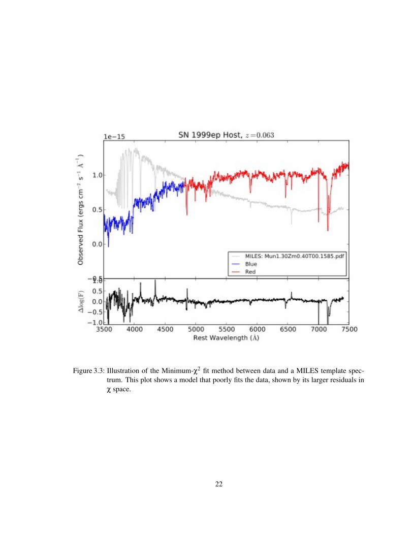
Figure 3.3: Illustration of the Minimum-χ2 fit method between data and a MILES template spec-trum. This plot shows a model that poorly fits the data, shown by its larger residuals inχ space.
22

Figure 3.4: Illustration of the Minimum-χ2 fit method between data and a MILES template spec-trum. This plot shows a model that is a better fit to the data. The residuals in thiscomparison are much smaller than Figure 3.3.
23

Figure 3.5: Illustration of the Minimum-χ2 fit method between data and a MILES template spec-trum. This plot shows a model that returned to be the minimum-χ2 for the data for SN1999ep. The residuals in χ space are the smallest out of every possible combination.
24

Figure 3.6: Contour plot, showing contour regions. The age and metallicity ranges were determinedby analyzing the darkest region. The white region shows the untested region due to lackof MILES spectra.
25

CHAPTER IV
Conclusions
4.1 Results & Discussion
The best fits and 1-σ regions for our 16 spectra are shown in Figure 4.1. These are only
conservative error estimates – in most cases the 1-σ regions were much smaller and less
symmetric. Also shown is the region in which Meng et al. would predict the most SNe
Ia would originate. From my comparison of data to synthetic spectra, I could not confirm
Meng’s prediction. I found that the events measured had the full range of available metal-
licities. This result, however, does not rule out the possibility of a metallicity dependence;
rather it implies a stronger dependence on age. Nearly 90% of our data points fell at an
age greater than 9 Gyr. These results are seemingly more supportive of an older progenitor
system, as indicated in Strolger et al. 2010.
The statistical certainty of my results appears to be at the 75% level. These results
are limited by the sample size and, possibly, by the method. We could potentially learn
more by increasing our sample size to contain more of the total sample or by changing
our library type (i.e. using PEGASE.2 models instead of MILES, to be discussed in Section
4.1.2). However, we have a sample size large enough to believe that the interpretation is
26

statistically robust.
Figure 4.1: Final plot with an estimation of Meng’s prediction region overlaid. Upper left of the plotwould include young, star-forming galaxies. Upper right of the plot would include old,star-forming galaxies. Bottom left of the plot would be unusual galaxies – young, butlacking in the metal content that one would expect with the increased metal abundancesin the universe (Note that this region was generally untestable due to the lack of MILESspectra). Bottom right of the plot would contain old, dying red galaxies that did notundergo many phases of star-formation.
27

4.1.1 Table of Ages and Metallicities
Host Age (Gyr) High Age Low Age Metallicity High Metallicity Low Metallicity(Gyr) (Gyr) [M/H] [M/H] [M/H]
99aq 0.7079 1.00 0.60 0.22 0.24 -0.2599ar 14.1254 14.5 12.5 -2.32 -2.32 -2.4099au 17.7828 18.0 14.0 0.00 0.20 -0.1599av 10.0000 18.0 6.50 -1.31 -1.25 -1.6099eo 10.0000 18.0 10.0 -2.32 -2.10 -2.4099ep 11.2202 12.0 9.00 -0.71 -0.60 -0.7599er 11.2202 15.0 8.00 -0.71 -0.65 -0.7500bn 11.2202 13.5 8.00 -1.31 -1.25 -1.7100em 10.0000 17.0 10.0 -2.32 -2.25 -2.4000eq 17.7828 13.0 14.0 0.00 0.25 -0.2000ff 10.0000 18.0 10.0 -2.32 -2.24 -2.4000fg 17.7828 13.0 15.0 0.00 0.10 -0.10
Barkley 11.2202 18.0 10.0 -1.71 -1.60 -2.00George 0.1122 0.30 0.10 -1.71 -1.00 -1.75Laurel 10.0000 10.3 10.0 -2.32 -2.25 -2.25Xenia 10.0000 10.5 10.0 -2.32 -2.25 -2.25
Table 4.1: Numerical findings from Age/Metallicity comparison.
4.1.2 Future Work
I have analyzed 16 host spectra out of a sample of approximately 60 available spectra.
The obvious next step is to attain ages and metallicities of the remaining test sample. I
anticipate that the remaining sample will either help to fill out the final plot or confirm the
stronger age dependence of these events.
In addition, it would be interesting to explore the possible use of potentially better
galactic models. The SSP models are more suited for modeling globular clusters than spi-
ral galaxies. In spiral galaxies, there is constant star formation and there are prominent
gas clouds, though useful in this current regard, are highly unphysical in that they do not
include gas content nor do they account for multiple age populations. It is incredibly im-
28

portant to account for gases present in the galaxy because the light from the stars in the
galaxy interacts with the gas, adding absorption and emission lines to the galactic spectra.
Additionally, the gas content provides an initial rate of star formation. Young, star-forming
galaxies would have more abundant gas clouds than old galaxies. Because of the presence
of gas absorption and emission lines, star-forming galaxies are more likely to match with
the wrong SSP model. These galaxies have many more features than we are testing for, both
in the emission and absorption, so the simplistic cross-correlation test is less robust than
the ideal test. One set of models that would be worth looking into would be the PEGASE.2
models.
Another place for improvement lies in the errors, specifically, the systematic error. One
question that we have yet to fully flesh out is this: How does the signal to noise ratio
affect the robustness of the cross-correlation test? It is inevitable that we attain error in any
measurement. The issue is not necessarily the signal-to-noise ratio, though it is always a
place for improvement. We do not fully know how the noise in the true data affected the
template fittings. Additionally, spectral combining could be a source of error. We took
multiple observations of the same galaxy, and combined the spectra to increase the signal-
to-noise ratio. However, when we only have three observations, and many extraneous
sources (bad pixels, cosmic rays, etc.) could taint our data, we opted to bias low by rejecting
the highest pixel, avoiding fake signal. This may have created false features in the spectra.
More investigation into the process of spectral combining is required to minimize these
errors.
The NGSS was a precursor to the Sloan Digital Sky Surveys. The surveys were de-
signed to look at galaxies, but had a piggy-back supernova detection operation. All of the
SDSS targets are low-z, within a comparable redshift to NGSS collection region. SDSS-II
29

detected 517 supernovae and 247 were spectroscopically identified as Type Ia (Dilday et
al. 2010). An excellent step up for my project would be to analyze these supernovae from
SDSS-II using the more robust PEGASE.2 models, should they prove to be effective. This
would bring our statistical error to 6%, near the 2-σ certainty region.
The effects of age and metallicity on SNe Ia production are important aspects to take
into consideration when determining the progenitor system of the events. However, these
are not the only particulars that play a part in that determination. A complimentary project
has explored ways to determine SN rates. These investigations will be included along with
the results discussed in this thesis in a forthcoming publication.
Scientists continue to search and observe and calculate. Time and again, we are met
with conflict, contradiction, and confusion instead of the comfort and clarity for which
we yearn. Is there hope for us as we seek to understand the nature of Dark Energy, this
mysterious force so intricately and cleverly integrated into the very fabric of the universe?
Time can only tell and it is traveling as fast as it can. As E. P. Hubble wrote of the initial
quest to measure cosmic expansion,
“Thus the explorations of space end on a note of uncertainty. And necessarily
so. We are, by definition, in the very center of the observable region. We know
our immediate neighborhood rather intimately. With increasing distance, our
knowledge fades, and fades rapidly. Eventually, we reach the dim boundary
– the utmost limits of our telescopes. There, we measure shadows, and we
search among ghostly errors of measurement for landmarks that are scarcely
more substantial. The search will continue. Not until the empirical resources
are exhausted, need we pass on to the dreamy realms of speculation.”
The Realm of the Nebulae
30

Chapter VIII (p. 202)Dover Publications, Inc. New York, New York, USA. 1958
31

BIBLIOGRAPHY
Bravo, E., & Badenes, C. 2011, Monthly Notices of the Royal Astronomical Society, 414, 1592
Filippenko A. V. 1997, Annual Review of Astronomy and Astrophysics, 35, 309
Gallagher et al. 2008, The Astrophysical Journal, 685, 749
Graves, G. & Shiavon. 2008, The Astrophysical Journal Supplement, 177, 446
Hamuy et al. 2000, The Astronomical Journal, 120, 1479
Howell et al. 2009, The Astrophysical Journal, 691, 661
Kobayashi C., Nomoto K., 2009, The Astrophysical Journal, 707, 1466
Maoz, D., Mannucci, F., Li, W., Filipenko, A. V., Della Valle, M., & Panagia, N. 2011, MonthlyNotices of the Royal Astronomical Society, 412, 1508
Meng, Xiang Cun; Li, Zhong Mu; Yang, Wu Ming 2011, Publications of the Astronomical Societyof the Pacific, 63, 31
Phillips M. M. 1993, The Astrophysical Journal, 431, 105
Pinto & Eastman 2000, The Astrophysical Journal, 530, 744
Perryman, M. A. C., et al. 1997, Astronomy and Astrophysics, 323, 49
Riess, A. . et al. 1998, The Astronomical Journal, 116, 1009
Strolger, L. -G., Dahlen, T., & Reiss, A. G. 2010, The Astrophysical Journal, 713, 32
Sullivan, M., et al. 2006, The Astrophysical Journal, 648, 868
Timmes et al. 2003, The Astrophysical Journal, 590, 83
Van Dyk, S. D., Li, W., & Filippenko, A. V. 2003, Publications of the Astronomical Society of thePacific. 115, 1259
Vazdekis et al. 2010, Monthly Notices of the Royal Astronomical Society, 404, 1639
Wolff, S. G. 2010, WKU Honors Thesis
32
Related Documents


![Supernova [PPT]](https://static.cupdf.com/doc/110x72/589d8c611a28ab6d4a8bb097/supernova-ppt.jpg)