The age of surface-exposed ice along the northern margin ...

The age of surface-exposed ice along the northern margin of the Greenland Ice SheetJoseph A. MacGregor 1, M.A. Fahnestock 2, W.T. Colgan 3, N.K. Larsen 4, K.K. Kjeldsen 3 and J.M. Welker 5,6

1 Cryospheric Sciences Lab (615), NASA GSFC; 2 Geophysical Inst., Univ. Alaska Fairbanks; 3 Geological Survey of Denmark and Greenland; 4 Globe Inst., Univ. Copenhagen 5 Dept. Biological Sciences, Univ. Alaska Anchorage; 6 Dept. of Ecology & Genetics, Univ. Oulu

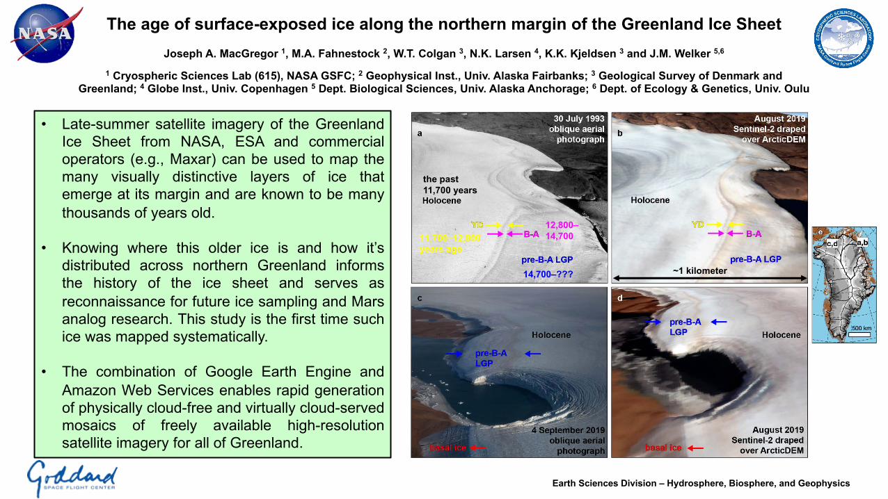
• Late-summer satellite imagery of the GreenlandIce Sheet from NASA, ESA and commercialoperators (e.g., Maxar) can be used to map themany visually distinctive layers of ice thatemerge at its margin and are known to be manythousands of years old.

• Knowing where this older ice is and how it’sdistributed across northern Greenland informsthe history of the ice sheet and serves asreconnaissance for future ice sampling and Marsanalog research. This study is the first time suchice was mapped systematically.

• The combination of Google Earth Engine andAmazon Web Services enables rapid generationof physically cloud-free and virtually cloud-servedmosaics of freely available high-resolutionsatellite imagery for all of Greenland.

Earth Sciences Division – Hydrosphere, Biosphere, and Geophysics

the past 11,700 years

11,700–12,800 years ago

12,800–14,700

14,700–??? ~1 kilometer

Name: Joseph A. MacGregor, Cryospheric Sciences Lab (Code 615), NASA GSFCE-mail: [email protected]: 301-614-5876

References:MacGregor, J.A., M.A. Fahnestock, W.T. Colgan, N.K. Larsen, K.K. Kjeldsen and J.M. Welker, The age of surface-exposed ice along the northern

margin of the Greenland Ice Sheet, Journal of Glaciology, 66(258), 667–684 doi:10.1017/jog.2020.62.Reeh, N., H. Oerter, and H. H. Thomsen (2002), Comparison between Greenland ice-margin and ice-core oxygen-18 records, Annals of

Glaciology, 35, 136–144, doi:10.3189/172756402781817365.

Data Sources: NASA MEaSUREs Greenland surface velocity, ESA Sentinel-2A/B, DigitalGlobe WorldView-2/3, NSF ArcticDEM and Greenland Ice Mapping Project (GIMP)

Technical Description of Figures:Figure 1: (A) Oblique aerial photograph of the northeastern margin of the Greenland Ice Sheet (same as Fig. 2 of Reeh et al., 2002), with Reeh et al. (2002)’s original age interpretation superimposed. Credit: H. Oerter. (B) August 2019 Sentinel-2 mosaic draped over 10-m ArcticDEM, with perspective and camera position oriented to approximately reproduce panel A, and Sentinel-2 colors contrast-stretched. No vertical exaggeration. (C) Oblique aerial photograph of northwestern margin of the Greenland Ice Sheet, with age interpretation superimposed. Note that the Younger Dryas (YD) and Bølling-Allerød (B-A) layers are only faintly visible there and were not traced; LGP: Last Glacial Period. Credit: J. Sonntag. (D) Same as panel B, but for site shown in panel C. (E) Map of Greenland showing site locations, where grayscale is surface speed (darker is faster).

Scientific significance, societal relevance, and relationships to future missions: This study sets the baseline for future studies of surface-exposed ice in Greenland and elsewhere – both remotely and in situ. We established a simple method for high-resolution, large-scale mosaic generation of value to mapping surface-exposed ice, we directly mapped layers of interest along thousands of kilometers of ice margin, and we directly compared this mapping against existing and new in situ measurements. This study’s results have broad implications for our understanding of the history of the Greenland Ice Sheet, where the most paleoclimatically interesting ice is exposed, the basal thermal state of northern Greenland, and where we might test future mission concepts for investigations of the polar layered deposits on Mars. We note that we primarily used Sentinel-2 for this study instead of Landsat-8 primarily due to the former’s finer resolution at visible wavelengths (10 vs. 15 m).


The Aerosol Characterization from Polarimeter and Lidar (ACEPOL) airborne field campaign Kirk Knobelspiesse1, Henrique M. J. Barbosa2,11, Christine Bradley3, Carol Bruegge3, Brian Cairns4, Gao Chen5, Jacek Chowdhary4,6, Anthony Cook5, Antonio Di Noia7,

Bastiaan van Diedenhoven4,6, David J. Diner3, Richard Ferrare5, Guangliang Fu8, Meng Gao1,9, Michael Garay3, Johnathan Hair5, David Harper5, Gerard van Harten3, Otto Hasekamp8, Mark Helmlinger3, Chris Hostetler5, Olga Kalashnikova3, Andrew Kupchock1,9, Karla Longo De Freitas1,15, Hal Maring10, J. Vanderlei Martins11, Brent McBride11,

Matthew McGill1, Ken Norlin12, Anin Puthukkudy11, Brian Rheingans3, Jeroen Rietjens8, Felix C. Seidel3,10, Arlindo da Silva1, Martijn Smit8, Snorre Stamnes5, Qian Tan13, Sebastian Val3, Andrzej Wasilewski4, Feng Xu14, Xiaoguang Xu11, John Yorks1

1NASA GSFC, 2U. of São Paulo, 3Jet Propulsion Laboratory, 4NASA GISS, 5NASA LARC, 6Columbia U., 7U. of Leicester, 8SRON Netherlands Institute for Space Research, 9SSAI, 10NASA Headquarters, 11U. of Maryland, Baltimore County, 12NASA AFRC, 13NASA ARC, 14U. of Oklahoma, 15USRA, (GSFC/GISS personnel in bold yellow)


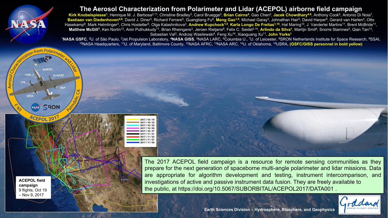
The 2017 ACEPOL field campaign is a resource for remote sensing communities as theyprepare for the next generation of spaceborne multi-angle polarimeter and lidar missions. Dataare appropriate for algorithm development and testing, instrument intercomparison, andinvestigations of active and passive instrument data fusion. They are freely available tothe public, at https://doi.org/10.5067/SUBORBITAL/ACEPOL2017/DATA001 .

ACEPOL field campaign9 flights, Oct 19 – Nov 9, 2017

Name: Kirk Knobelspeisse, Ocean Ecology Laboratory, 616, NASA GSFCE-mail: [email protected]: (301) 614-6242

References:Knobelspiesse, K., Barbosa, H. M. J., Bradley, C., Bruegge, C., Cairns, B., Chen, G., Chowdhary, J., Cook, A., Di Noia, A., van Diedenhoven, B., Diner, D. J., Ferrare, R., Fu, G., Gao, M., Garay, M., Hair, J., Harper, D., van Harten, G., Hasekamp, O., Helmlinger, M., Hostetler, C., Kalashnikova, O., Kupchock, A., Longo De Freitas, K., Maring, H., Martins, J. V., McBride, B., McGill, M., Norlin, K., Puthukkudy, A., Rheingans, B., Rietjens, J., Seidel, F. C., da Silva, A., Smit, M., Stamnes, S., Tan, Q., Val, S., Wasilewski, A., Xu, F., Xu, X., and Yorks, J.: The Aerosol Characterization from Polarimeter and Lidar (ACEPOL) airborne field campaign, Earth System Science Data., https://doi.org/10.5194/essd-2020-76, in press, 2020.

Data Sources:

Technical Description of Figures:Background: Photograph from the ER-2 of smoke from prescribed burns in Kaibab National Forest in Arizona on November 9th, 2017. Credit: NASA/Stu Broce. Top left: The ACEPOL field campaign emblem, which also shows the positions of instruments onboard the ER-2 aircraft. Bottom left: Flight tracks. Nine were conducted from October 19th to November 9th, 2017 over California, Nevada, Arizona, New Mexico and the coastal Pacific Ocean from the Armstrong Flight Research Center in Palmdale, California. Image mapped using Google Earth, © 2018 Google.

Scientific significance, societal relevance, and relationships to future missions: ACEPOL flew four multi-angle polarimeters and two lidars in a variety of conditions, collecting a dataset ideal for instrument and algorithm development, relevant to missions such as PACE and A-CCP.


Archive URL, DOIPrimary: ASDC https://asdc.larc.nasa.gov/project/ACEPOL, 10.5067/SUBORBITAL/ACEPOL2017/DATA001AirMSPI

instrument

https://eosweb.larc.nasa.gov/project/airmspi/airmspi_table, 10.5067/AIRCRAFT/AIRMSPI/ACEPOL/RADIANCE/ELLIPSOID_V006

10.5067/AIRCRAFT/AIRMSPI/ACEPOL/RADIANCE/TERRAIN_V006GroundMSPI

instrument

https://eosweb.larc.nasa.gov/project/airmspi/airmspi_table, 10.5067/GROUND/GROUNDMSPI/ACEPOL/RADIANCE_v009

Phytoplankton are a diverse set of organisms with varying effects on the marine food web. However, standard NASA satelliteproducts do not estimate the abundance of different species. We develop an algorithm using ship-based observations to predictthe abundance of three key phytoplankton types: Prochlorococcus, Synechococcus, and autotrophic picoeukaryotes. We applythis algorithm to satellite data and show, for the first time, an estimate of their abundances throughout the Atlantic Ocean.


New satellite algorithm estimates abundances of the smallest phytoplankton speciesPriscila K. Lange,1,2,3 P. Jeremy Werdell,1 Zachary K. Erickson,1,4 Susanne E. Craig,1,2 Ivona Cetinić,1,2 and others

1Ocean Ecology Laboratory, NASA GSFC; 2USRA; 3Blue Marble Space Institute of Science; 4NASA Postdoctoral Program

Name: Ivona Cetinić, Ocean Ecology Laboratory (Code 616.0), NASA GSFC/USRAE-mail: [email protected]: 301-286-1514

References:Priscila K. Lange, P. Jeremy Werdell, Zachary K. Erickson, Giorgio Dall’Olmo, Robert J. W. Brewin, Mikhail V. Zubkov, Glen A. Tarran, Heather A. Bouman,Wayne H. Slade, Susanne E. Craig, Nicole J. Poulton, Astrid Bracher, Michael W. Lomas, Ivona Cetinić, 2020. Radiometric approach for the detection of picophytoplankton assemblages across oceanic fronts, Optics Express, doi: 10.1364/OE.398127.

Full affiliation list: Ocean Ecology Laboratory, NASA GSFC (PKL, PJW, ZKE, SEC, IC); Universities Space Research Association (SEC, IC); Blue Marble Space Institute of Science (PKL); NASA Postdoctoral Program (ZKE); National Centre for Earth Observation, Plymouth Marine Laboratory, United Kingdom (GD, GAT); College of Life and Environmental Sciences, University of Exeter, United Kingdom (RJWB); Scottish Association for Marine Science, Scotland (MVZ); Department of Earth Sciences, University of Oxford, United Kingdom (HAB); Sequoia Scientific, USA (WS); Bigelow Laboratory for Ocean Sciences, USA (NJP, MWL); Climate Sciences, Alfred Wegener Institute Helmholtz Centre for Polar and Marine Research, Germany (AB); Institute of Environmental Physics, Department of Physics and Electrical Engineering, University of Bremen, Germany (AB)

Data Sources: Ship-based observations from the Atlantic Meridional Transect Program (AMT; United Kingdom) and distributed by the British Oceanographic Data Centre (BODC). Aqua MODIS satellite data processed and distributed by the NASA Ocean Biology Processing Group (OBPG). We are thankful to all the scientists that contributed to collection of this dataset, the captains and crews of all the research vessels that supported these and our other sea-going adventures, and to Erdem Karaköylü for valuable advice on the use of statistical methods.

Technical Description of Figure: Ship-based observations from AMT were used to develop an algorithm using principal component analysis (PCA) to relate remote sensing reflectances at seven different wavelengths, as well as radiometrically-derived sea surface temperature (SST), to surface abundances of three phytoplankton groups: (a) Prochlorococcus, (b) Synechococcus, and (c) autotrophic picoeukaryotes. This model was validated using AMT data withheld from the algorithm development, and then applied to Aqua MODIS data to estimate abundances of these three phytoplankton groups throughout the Atlantic Ocean. Data from October 2014 are shown to match when the AMT datasets were collected. Pixels with no valid Aqua MODIS measurements during this month are white.

Scientific significance, societal relevance, and relationships to future missions: Different phytoplankton groups have varying contributions to primary production, carbon sequestration and export, and fishery stocks. In addition, Synechococcus, a unicellular cyanobacteria, typically exists in narrow filaments, or fronts, that separate different boundaries in oceanic ecosystems; thus, satellite observations of Synechococcus may help map where these boundaries are and how they shift over time. This research therefore directly addresses the Decadal Survey Scientific Priority E-1: “What are the structure, function, and biodiversity of Earth’s ecosystems, and how and why are they changing in time and space?” (ESAS 2017). This research finds an improved model performance using hyperspectral reflectance data, which will be measured as part of the upcoming NASA PACE (Plankton, Aerosol, Clouds, ocean Ecosystem) satellite mission.


Global GRACE/GRACE-FO data assimilation for groundwater and drought monitoringBailing Li, Matthew Rodell, Sujay Kumar, Hiroko Beaudoing, Augusto Getirana, Natthachet Tangdamrongsub, Frederick Policelli and David Mocko

Code 617/Hydrological Sciences Laboratory

The Gravity Recovery and Climate Experiment (GRACE) and GRACE Follow On (GRACE-FO) satellite missions areunique in their ability to observe changes in all forms of water stored on and beneath the land surface. By combiningthese observations with other data within a numerical model (i.e., data assimilation) we can spatially and temporallydownscale the observations and produce results in near real time, making maps that are useful for groundwater anddrought monitoring (shown above). Evaluation using situ observations proves that GRACE and GRACE-FO dataassimilation significantly improve the results over modeling alone.


Nearly 4,000 in situ wells in five continents

Regional scale

RMSE down by 36%

Correlation up by 16%

Point scale

RMSE down by 10%

Correlationup by 22%

Evaluation results(RMSE: root mean square error)

Name: Bailing Li, Hydrological Sciences Laboratory, NASA GSFC E-mail: [email protected]: 301-286-6020

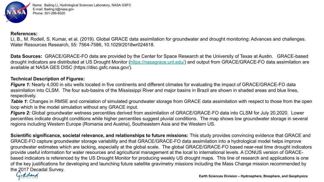
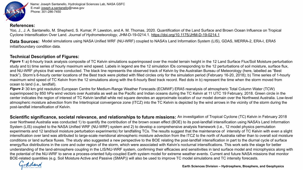
References:Li, B., M. Rodell, S. Kumar, et al. (2019). Global GRACE data assimilation for groundwater and drought monitoring: Advances and challenges. Water Resources Research, 55: 7564-7586, 10.1029/2018wr024618.

Data Sources: GRACE/GRACE-FO data are provided by the Center for Space Research at the University of Texas at Austin. GRACE-based drought indicators are distributed at US Drought Monitor (https://nasagrace.unl.edu/) and output from GRACE/GRACE-FO data assimilation are available at NASA GES DISC (https://disc.gsfc.nasa.gov/).

Technical Description of Figures:Figure 1: Nearly 4,000 in situ wells located in five continents and different climates for evaluating the impact of GRACE/GRACE-FO data assimilation into CLSM. The four sub-basins of the Mississippi River and major basins in Brazil are shown in shaded areas and blue lines, respectively. Table 1: Changes in RMSE and correlation of simulated groundwater storage from GRACE data assimilation with respect to those from the open loop which is the model simulation without any GRACE input. Figure 2: Global groundwater wetness percentiles derived from assimilation of GRACE/GRACE-FO data into CLSM for July 20,2020. Lower percentiles indicate drought conditions while higher percentiles suggest pluvial conditions. The map shows low groundwater storage in several regions including Western Europe (Romania and Austria), Southeastern Asia and the Western US.

Scientific significance, societal relevance, and relationships to future missions: This study provides convincing evidence that GRACE and GRACE-FO capture groundwater storage variability and that GRACE/GRACE-FO data assimilation into a hydrological model helps improve groundwater estimates which are lacking, especially at the global scale. The global GRACE/GRACE-FO based near-real time drought indicators provide useful information for water resources and agricultural management at the local to international levels. A CONUS version of GRACE-based indicators is referenced by the US Drought Monitor for producing weekly US drought maps. This line of research and applications is one of the key justifications for developing and launching future satellite gravimetry missions including the Mass Change mission recommended by the 2017 Decadal Survey.


https://nasagrace.unl.edu/

Quantification of the Land Surface and ‘Brown Ocean’ Influence on Tropical Cyclone Intensification Over Land

Jinwoong Yoo1,2, Joseph A. Santanello, Jr.2, Marshall Shepherd3, Sujay Kumar2, Patricia Lawston1,2, and Andrew M. Thomas31ESSIC-UMCP, 2Hydrological Sciences Lab, NASA-GSFC, 3University of Georgia

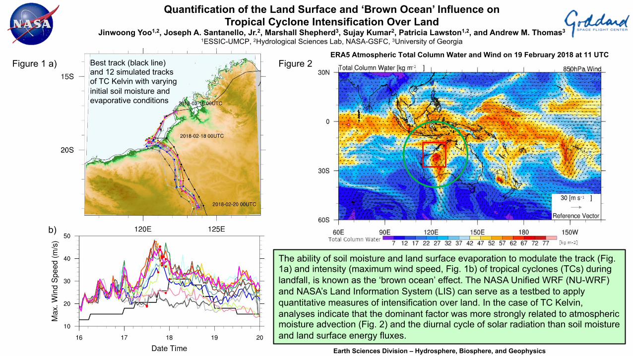
The ability of soil moisture and land surface evaporation to modulate the track (Fig. 1a) and intensity (maximum wind speed, Fig. 1b) of tropical cyclones (TCs) during landfall, is known as the ‘brown ocean’ effect. The NASA Unified WRF (NU-WRF) and NASA’s Land Information System (LIS) can serve as a testbed to apply quantitative measures of intensification over land. In the case of TC Kelvin, analyses indicate that the dominant factor was more strongly related to atmospheric moisture advection (Fig. 2) and the diurnal cycle of solar radiation than soil moisture and land surface energy fluxes.


Figure 1 a) Best track (black line) and 12 simulated tracks of TC Kelvin with varying initial soil moisture and evaporative conditions

Figure 2

b)

ERA5 Atmospheric Total Column Water and Wind on 19 February 2018 at 11 UTC

Name: Joseph Santanello, Hydrological Sciences Lab, NASA GSFCE-mail: [email protected]: 301-286-7450

References:Yoo, J., J. A. Santanello, M. Shepherd, S. Kumar, P. Lawston, and A. M. Thomas, 2020. Quantification of the Land Surface and Brown Ocean Influence on Tropical Cyclone Intensification Over Land. Journal of Hydrometeorology, JHM-D-19-0214.1. https://doi.org/10.1175/JHM-D-19-0214.1

Data Sources: Model simulations using NASA Unified WRF (NU-WRF) coupled to NASA’s Land Information System (LIS), GDAS, MERRA-2, ERA-I, ERA5 initial/boundary condition data.

Technical Description of Figures:Figure 1: a) 6-hourly track analysis composite of TC Kelvin simulations superimposed over the model terrain height in the 12 Land Surface Flux/Soil Moisture perturbation study and b) time series of hourly maximum wind speed. Labels in legend are the 12 simulation IDs corresponding to the 12 perturbations of soil moisture, surface flux, and NU-WRF physics that were conducted. The black line represents the observed track of Kelvin by the Australian Bureau of Meteorology (here, labelled as “Best track”). Storm’s 6-hourly center locations of the Best track were plotted with filled circles only for the simulation period (February 16-20, 2018); b) Time series of 1-hourly maximum wind speed of TC Kelvin from the 12 simulations along with the 6-hourly Best track record. Red dots in b) represent the time when the storm moved from ocean to land (i.e., landfall). Figure 2: 30 km grid resolution European Centre for Medium-Range Weather Forecasts (ECMWF) ERA5 reanalysis of atmospheric Total Column Water (TCW) superimposed by 850 hPa wind vectors over Australia as well as the Pacific and Indian oceans during the TC Kelvin at 11 UTC 19 February, 2018. Green circle in the center indicates the region of interest of TC Kelvin landfall while red square denotes an approximate location of our model domain over the Northwest Australia. Low-level atmospheric moisture advection from the Intertropical convergence zone (ITCZ) into the TC Kelvin is depicted by the wind arrows in the vicinity of the storm during the post-landfall intensification of Kelvin.

Scientific significance, societal relevance, and relationships to future missions: An investigation of Tropical Cyclone (TC) Kelvin in February 2018 over Northwest Australia was conducted 1) to quantify the contribution of the brown ocean effect (BOE) to its post-landfall intensification using NASA’s Land Information System (LIS) coupled to the NASA Unified WRF (NU-WRF) system and 2) to develop a comprehensive analysis framework (i.e., 12 model physics permutation experiments and 12 land/soil moisture perturbation experiments) for landfalling TCs. The results suggest that the maintenance of intensity of TC Kelvin with even a slight intensification over land was attributed to large-scale meridional atmospheric moisture advection from the ITCZ to the north of Australia rather than to overall soil moisture conditions or land surface fluxes. The study also suggested a new perspective to the BOE relating the post-landfall intensification in part to the diurnal cycle of surface energy/flux distributions in the core and outer region of the storm, which were associated with Kelvin’s nocturnal intensifications. This work sets the stage for better understanding of the land-atmosphere coupling in the LIS/NU-WRF system, confirming their efficacies and sensitivities in land surface model and microphysics along with the potential of the NU-WRF to serve a process-oriented fully-coupled Earth system model for extreme weather events. Current and future NASA missions that monitor BOE-related quantities (e.g. Soil Moisture Active and Passive (SMAP)) will also be used to improve TC model simulations and TC intensity forecasts.


mailto:[email protected]

https://doi.org/10.1175/JHM-D-19-0214.1

Accurate simulations of surface reflectance from a dynamic forest modelShiklomanov, A.N.1, Dietze, M.C.2, Fer, I.3, Viskari, T.3, Serbin, S4

1NASA Goddard Space Flight Center, 2Boston University, 3Finnish Meteorological Institute, 4Brookhaven National Laboratory

We modified a computer model of forest growth and competition to also predict surface reflectancespectra as observed by airborne and satellite remote sensing. This model was able to accurately simulateairborne measurements of surface reflectance across a variety of sites in the US Upper Midwest. Thisgives us a way to train and test models against remote sensing data without relying on derived remotesensing data products.


Model

Airborne observation

Name: Alexey N. Shiklomanov, 6180, NASA GSFCE-mail: [email protected]: 240-784-9862

References:• Shiklomanov, AN. ”Improving ecological forecasts using model and data constraints”. PhD Dissertation, Dept. of Earth & Environment,

Boston University. https://hdl.handle.net/2144/32714• Viskari, T.; Shiklomanov, AN.; Dietze, MC; and Serbin, SP. “The Influence of Canopy Radiation Parameter Uncertainty on Model Projections

of Terrestrial Carbon and Energy Cycling.” PLOS ONE 14, no. 7 (July 2019): e0216512. DOI:10.1371/journal.pone.0216512.• Shiklomanov, AN; Dietze, MC; Fer, I; Viskari, T.; Serbin, SP. “Cutting out the middleman: Calibrating and validating a dynamic vegetation

model using remotely sensed surface reflectance”. Geoscientific Model Development. In prep.

Data Sources: NASA Airborne Visible / InfraRed Imaging Spectrometer – Classic (AVIRIS-Classic) surface reflectance. Forest survey data from NASA Forest Functional Types (FFT) field campaign. Ecosystem Demography Model v2 (ED2).

Technical Description of Figures:(Left) Map of sites used for model calibration, with example sites highlighted in red. (Center) 3D visualization of Ecosystem Demography (ED) model state at the time of surface reflectance simulation. Colors and geometries represent different plant functional types coexisting in the same space, and heights and canopy sizes are proportional to corresponding variables in the model. (Right) Comparison of surface reflectance simulated using ED (green) and observed by the AVIRIS-Classic. Surface reflectance is simulated by coupling the canopy radiative transfer model internal to ED (used to determine canopy light availability and to drive biophysical processes) with the PROSPECT 5 leaf spectral model.

Scientific significance, societal relevance, and relationships to future missions: Vegetation models are often calibrated and validated against derived remote sensing data products (e.g., leaf area index, LAI, derived from the Moderate Resolution Imaging Spectroradiometer, MODIS). However, these products are generally based on models of their own, which can introduce considerable uncertainties into the validation. This approach not only reduces uncertainties associated with derived products, but also provides a way for ED and similar models to leverage spectral data at any spectral resolution, including hyperspectral observations from the NASA Goddard’s LiDAR, Hyperspectral, and Thermal Imager (G-LiHT) and the forthcoming Surface Biology and Geology (SBG) designated observable.


First GRACE Gravitational Measurements of Tsunamis

Ghobadi-Far, K.1, S.C. Han1, S. Allgeyer2, P. Tregoning2, J.Sauber3,S. Behzadpour4, T. Mayer-Gürr4, N. Sneeuw5, and E. Okal6

1University of Newcastle, Australia, 2Australian National University, Australia, 3NASA GSFC, MD, USA, 4Graz University of Technology, Austria, 5University of Stuttgart, Germany, 6Northwestern University, IL, USA

Large tsunamis in the open ocean cause sea level change of a few decimeters over wavelengths of hundreds of kilometers. Tsunamisgenerated by the 2004 M9.2 Sumatra, 2010 M8.8 Maule, and 2011 M9.0 Tohoku caused the trajectory of Gravity Recovery and ClimateExperiment (GRACE) satellites at ~500 km above the Earth’s surface to be significantly perturbed. These GRACE tsunami observationsare being used to improve tsunami model simulation and prediction and for studying the mechanisms of large tsunamis.


Line-of-sight gravity difference (LGD)

Name: Jeanne Sauber, 61A, NASA GSFCE-mail: [email protected]: 301-614-6465

References:

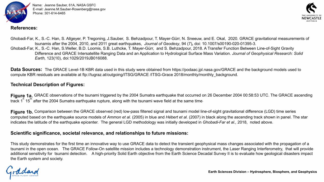
Ghobadi-Far, K., S.-C. Han, S. Allgeyer, P. Tregoning, J.Sauber, S. Behzadpour, T. Mayer-Gürr, N. Sneeuw, and E. Okal, 2020. GRACE gravitational measurements of tsunamis after the 2004, 2010, and 2011 great earthquakes, Journal of Geodesy, 94 (7), doi: 10.1007/s00190-020-01395-3.

Ghobadi-Far, K., S.-C. Han, S.Weller, B.D. Loomis, S.B. Luthcke, T. Mayer-Gürr, and S. Behzadpour, 2018. A Transfer Function Between Line-of-Sight Gravity Difference and GRACE Intersatellite Ranging Data and an Application to Hydrological Surface Mass Variation. Journal of Geophysical Research: Solid Earth, 123(10), doi:1029/2019JB016088.

Data Sources: The GRACE Level-1B KBR data used in this study were obtained from https://podaac.jpl.nasa.gov/GRACE and the background models used to compute KBR residuals are available at ftp://tugraz.at/outgoing/ITSG/GRACE /ITSG-Grace 2018/monthly/monthly_background.

Technical Description of Figures:

Figure 1a. GRACE observations of the tsunami triggered by the 2004 Sumatra earthquake that occurred on 26 December 2004 00:58:53 UTC. The GRACE ascending track 1h 15m after the 2004 Sumatra earthquake rupture, along with the tsunami wave field at the same time.

Figure 1b. Comparison between the GRACE observed (red) low-pass filtered signal and tsunami model line-of-sight gravitational difference (LGD) time series computed based on the earthquake source models of Ammon et al. (2005) in blue and Hébert et al. (2007) in black along the ascending track shown in panel. The star indicates the latitude of the earthquake epicenter. The general LGD methodology was initially developed in Ghobadi-Far et al., 2018, noted above.

Scientific significance, societal relevance, and relationships to future missions:

This study demonstrates for the first time an innovative way to use GRACE data to detect the transient geophysical mass changes associated with the propagation of a tsunami in the open ocean. The GRACE Follow-On satellite mission includes a technology demonstration instrument, the Laser Ranging Interferometry, that will provide additional sensitivity for tsunami detection. A high-priority Solid Earth objective from the Earth Science Decadal Survey II is to evaluate how geological disasters impact the Earth system and society.


Lake and Reservoir Volume Variations in South America from Radar Altimetry, ICESat Laser Altimetry, and GRACE Time-variable Gravity

Claudia C. Carabajal 1 and J.-P. Boy 2

1 Hexagon US Federal, Geodesy and Geophysics Lab, NASA Goddard Space Flight Center, Greenbelt, MD, USA.2 EOST/IPGS (UMR 7516 CNRS – Université de Strasbourg), Strasbourg, France.

Lake and reservoir water levels, extent and storage can be remotely monitored by radar and laser altimetry (e.g. ICESat), imagery (e.g.MODIS), and time-variable gravity (e.g. GRACE) over several decades. High-resolution GRACE mascons enable monitoring small lakeand reservoir water storage variations. These valuable measurements of the hydrological cycle continue with various Radar Altimetrymissions, ICESat-2 (launched in September 2018), GEDI (launched December 2018), Imaging Spectrometers, gravity missions likeGRACE Follow-On (launched in May 2018), and future missions like SWOT (launch planned for September 2021).


Fig. 1: Lake Chiquita (Argentina) water extent. Fig. 2: Lake Chiquita water height and volume.

ICESat - Ice, Cloud and land Elevation Satellite

MODIS - Moderate Resolution Imaging Spectroradiometer

GRACE - Gravity Recovery And Climate Experiment

GEDI – Global Ecosystem Dynamics Investigation

SWOT – Surface Water and Ocean Topography

Name: Claudia C. Carabajal, Geodesy and Geophysics Lab, Hexagon US Federal @ NASA GSFCE-mail: [email protected]: 301.614.6111

References:Carabajal, C. C. and J.-P. Boy, 2020. Lake and Reservoir Volume Variations in South America from Radar Altimetry, ICESat Laser Altimetry, and GRACE time-variable gravity, Advances in

Space Research, doi: 10.1016/j.asr.2020.04.022

Data Sources: MODIS MOD13Q1 NDVI v006, https://lpdaac.usgs.gov/products/mod13q1v006/.PO.DAAC, https://podaac.jpl.nasa.gov/dataset/PRESWOT_HYDRO_L3_LAKE_RESEVOIR_AREA_V2.

ICESat (Ice Cloud and Land Elevation Satellite) GLA14 (Edited) Laser Altimetry Datasets, https://nsidc.org/data/GLAH14/versions/34.

GREALM: https://ipad.fas.usda.gov/cropexplorer/global_reservoir/.DAHITI: https://dahiti.dgfi.tum.de/en/.HYDROWEB: http://hydroweb.theia-land.fr/?lang=en&.

GRACE (Gravity Recovery and Climate Experiment) Global Mascons v02.4, https://earth.gsfc.nasa.gov/geo/data/grace-mascons.

In Situ Water Level Data (Sistema Nacional de Información Hídrica), https://snih.hidricosargentina.gob.ar/.

Technical Description of Figures:Figure 1: Top: Time series of surface area variations (km2) for lake Chiquita (Argentina). In black, our estimates using MODIS NDVI products are shown, along with Crétaux et al. (2011) results, in green. High (2003/10/16) and low (2009/03/22) surface extents are shown with a red dot, corresponding to L2A and L2E ICESat laser periods observations. Bottom: Map of MODIS NDVI for the two extremes of surface extent shown above with the red dots. ICESat tracks for L2A and L2E are shown, with elevations sampled shown be the color bar at the bottom.

Figure 2: Top: ICESat water elevation (m) for lake Chiquita, compared to radar altimetry (Hydroweb) results from Crétaux et al. (2011). Bottom: Comparison of volume variations from GRACE mascons (red), from MODIS and altimetry (our results, shown in black using our hypsometry with ICESat water levels, and in blue using our hypsometry with water levels from Hydroweb), and Crétaux et al. (2011) volume estimates (green).

Scientific significance, societal relevance, and relationships to future missions: Lake water storage is an important component of the water cycle, a key parameter in understanding and modelling the climate variably, and a critical resource for society. The study compares and validates different estimates of water storage variations from various space observations (radar and laser altimetry, imagery, and time-variable gravity), and in situ measurements, focusing on South America. High resolution mascon solutions developed at NASA/GSFC are able to fully recover lake mass variations for water bodies of small spatial extent. Current laser altimetry data products from NASA missions, like ICESat-2 and GEDI (Global Ecosystem Dynamics Investigation), provide valuable data to combine with GRACE Follow-On water storage estimates using similar approaches, facilitating synergetic use of these observations, and the validation of future mission products like those that will be provided by the SWOT mission.


The age of surface-exposed ice along the northern margin ...

Documents