The (2,2,0) Drazin Inverse Problem P. Patr´ ıcio a* and R.E. Hartwig b a Departamento de Matem´ atica e Aplica¸ c˜ oes, Universidade do Minho, 4710-057 Braga, Portugal. E-mail: [email protected] b Mathematics Department, N.C.S.U., Raleigh, NC 27695-8205, U.S.A. E-mail: [email protected] Abstract We consider the additive Drazin problem and we study the existence of the Drazin inverse of a two by two matrix with zero (2,2) entry. Keywords: Drazin inverse, block matrices AMS classification: 15A09, 16E50 1 Introduction Unless otherwise stated, all elements are in a ring R with unity 1. The Drazin inverse (D-inverse, for short) of a, denoted by a d , is the unique solution to the equations a k+1 x = a k , xax = x, ax = xa, for some k ≥ 0, if any. The minimal such k is called the index, denoted in(a), of a. If the Drazin inverse exists, we shall call the element D-invertible, or strongly-pi-regular. When in(a) ≤ 1, we say a has a group inverse, denoted by a # . We say a ∈ R is regular if a ∈ aRa. We shall need the concept of regularity, which guarantees solutions to aa - a = a and aa + a = a, a + = a + aa + . a - is called an inner inverse of a, and a + is called a reflexive inverse of a. Two elements x and y are said to be left(right) orthogonal (LO/RO), if xy = 0 (resp. yx = 0), and orthogonal, denoted by x ⊥ y, if xy = yx = 0. Semi-orthogonality means either LO or RO. If a is D-invertible, then a =(a 2 a d )+ a(1 - aa d )= c a + n a is referred as the core-nilpotent decomposition of a. Note that c a ⊥ n a , n a is nilpotent, and a d = c # a . R. Cline showed in [7] how to relate (ab) d with (ba) d , namely (ab) d = a[(ba) d ] 2 b. This equality is known as Cline’s formula. In this paper, we shall examine the representation of the Drazin inverses of the block matrix M = a c b 0 , in which the (2,2) entry is zero. We aim for results in terms of “words” in a, b * Corresponding author 1

Welcome message from author
This document is posted to help you gain knowledge. Please leave a comment to let me know what you think about it! Share it to your friends and learn new things together.
Transcript

The (2,2,0) Drazin Inverse Problem
P. Patrıcioa∗and R.E. Hartwigb
aDepartamento de Matematica e Aplicacoes, Universidade do Minho, 4710-057 Braga, Portugal.
E-mail: [email protected] Department, N.C.S.U., Raleigh, NC 27695-8205, U.S.A. E-mail: [email protected]
Abstract
We consider the additive Drazin problem and we study the existence of the Drazin
inverse of a two by two matrix with zero (2,2) entry.
Keywords: Drazin inverse, block matrices
AMS classification: 15A09, 16E50
1 Introduction
Unless otherwise stated, all elements are in a ring R with unity 1.
The Drazin inverse (D-inverse, for short) of a, denoted by ad, is the unique solution to the
equations ak+1x = ak, xax = x, ax = xa, for some k ≥ 0, if any. The minimal such k is
called the index, denoted in(a), of a. If the Drazin inverse exists, we shall call the element
D-invertible, or strongly-pi-regular. When in(a) ≤ 1, we say a has a group inverse, denoted by
a#.
We say a ∈ R is regular if a ∈ aRa. We shall need the concept of regularity, which
guarantees solutions to aa−a = a and aa+a = a, a+ = a+aa+. a− is called an inner inverse of
a, and a+ is called a reflexive inverse of a.
Two elements x and y are said to be left(right) orthogonal (LO/RO), if xy = 0 (resp.
yx = 0), and orthogonal, denoted by x ⊥ y, if xy = yx = 0. Semi-orthogonality means either
LO or RO.
If a is D-invertible, then a = (a2ad) + a(1− aad) = ca + na is referred as the core-nilpotent
decomposition of a. Note that ca ⊥ na, na is nilpotent, and ad = c#a .
R. Cline showed in [7] how to relate (ab)d with (ba)d, namely (ab)d = a[(ba)d]2b. This
equality is known as Cline’s formula.
In this paper, we shall examine the representation of the Drazin inverses of the block matrix
M =
[a c
b 0
], in which the (2,2) entry is zero. We aim for results in terms of “words” in a, b
∗Corresponding author
1
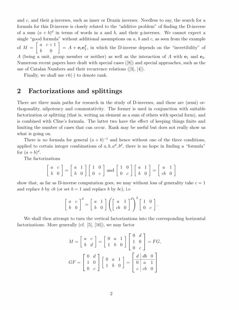
and c, and their g-inverses, such as inner or Drazin inverses. Needless to say, the search for a
formula for this D-inverse is closely related to the “additive problem” of finding the D-inverse
of a sum (a + b)d in terms of words in a and b, and their g-inverses. We cannot expect a
single “good formula” without additional assumptions on a, b and c, as seen from the example
of M =
[a c+ 1
b 0
]= A + e1e
T2 , in which the D-inverse depends on the “invertibility” of
A (being a unit, group member or neither) as well as the interaction of A with e1 and e2.
Numerous recent papers have dealt with special cases ([8]) and special approaches, such as the
use of Catalan Numbers and their recurrence relations ([3], [4]).
Finally, we shall use rk(·) to denote rank.
2 Factorizations and splittings
There are three main paths for research in the study of D-inverses, and these are (semi) or-
thogonality, nilpotency and commutativity. The former is used in conjunction with suitable
factorization or splitting (that is, writing an element as a sum of others with special form), and
is combined with Cline’s formula. The latter two have the effect of keeping things finite and
limiting the number of cases that can occur. Rank may be useful but does not really show us
what is going on.
There is no formula for general (a + b)−1 and hence without one of the three conditions,
applied to certain integer combinations of a, b, ad, bd, there is no hope in finding a “formula”
for (a+ b)d.
The factorizations[a c
b 0
]=
[a 1
b 0
] [1 0
0 c
]and
[1 0
0 c
] [a 1
b 0
]=
[a 1
cb 0
]show that, as far as D-inverse computation goes, we may without loss of generality take c = 1
and replace b by cb (or set b = 1 and replace b by bc), i.e
[a c
b 0
]d=
[a 1
b 0
]([a 1
cb 0
]d)2 [1 0
0 c
].
We shall then attempt to turn the vertical factorizations into the corresponding horizontal
factorizations. More generally (cf. [5], [16]), we may factor
M =
[a c
b d
]=
[0 a 1
1 b 0
] 0 d
1 0
0 c
= FG,
GF =
0 d
1 0
0 c
[ 0 a 1
1 b 0
]=
d db 0
0 a 1
c cb 0
2
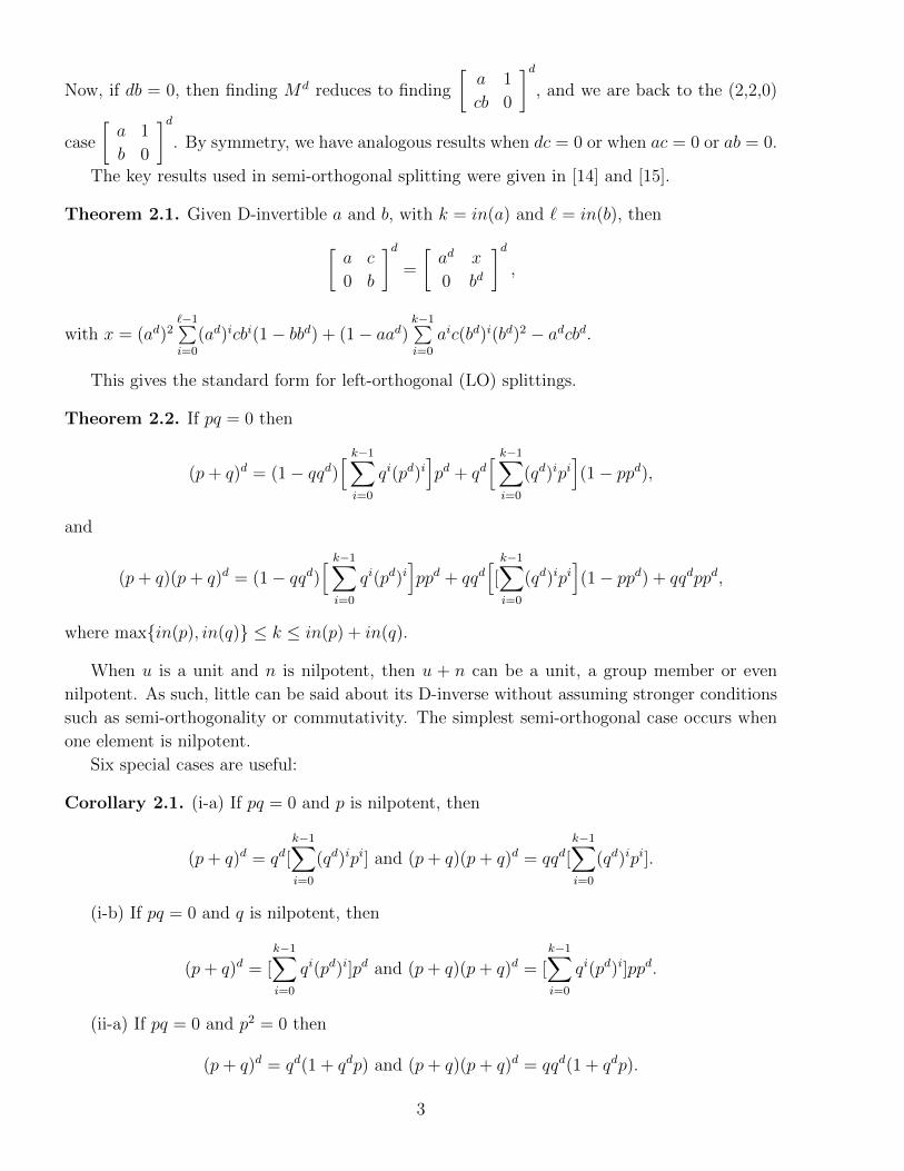
Now, if db = 0, then finding Md reduces to finding
[a 1
cb 0
]d, and we are back to the (2,2,0)
case
[a 1
b 0
]d. By symmetry, we have analogous results when dc = 0 or when ac = 0 or ab = 0.
The key results used in semi-orthogonal splitting were given in [14] and [15].
Theorem 2.1. Given D-invertible a and b, with k = in(a) and ` = in(b), then[a c
0 b
]d=
[ad x
0 bd
]d,
with x = (ad)2`−1∑i=0
(ad)icbi(1− bbd) + (1− aad)k−1∑i=0
aic(bd)i(bd)2 − adcbd.
This gives the standard form for left-orthogonal (LO) splittings.
Theorem 2.2. If pq = 0 then
(p+ q)d = (1− qqd)[ k−1∑i=0
qi(pd)i]pd + qd
[ k−1∑i=0
(qd)ipi](1− ppd),
and
(p+ q)(p+ q)d = (1− qqd)[ k−1∑i=0
qi(pd)i]ppd + qqd
[[k−1∑i=0
(qd)ipi](1− ppd) + qqdppd,
where max{in(p), in(q)} ≤ k ≤ in(p) + in(q).
When u is a unit and n is nilpotent, then u + n can be a unit, a group member or even
nilpotent. As such, little can be said about its D-inverse without assuming stronger conditions
such as semi-orthogonality or commutativity. The simplest semi-orthogonal case occurs when
one element is nilpotent.
Six special cases are useful:
Corollary 2.1. (i-a) If pq = 0 and p is nilpotent, then
(p+ q)d = qd[k−1∑i=0
(qd)ipi] and (p+ q)(p+ q)d = qqd[k−1∑i=0
(qd)ipi].
(i-b) If pq = 0 and q is nilpotent, then
(p+ q)d = [k−1∑i=0
qi(pd)i]pd and (p+ q)(p+ q)d = [k−1∑i=0
qi(pd)i]ppd.
(ii-a) If pq = 0 and p2 = 0 then
(p+ q)d = qd(1 + qdp) and (p+ q)(p+ q)d = qqd(1 + qdp).
3
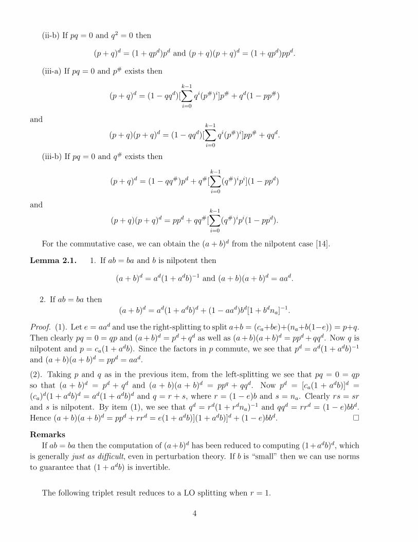
(ii-b) If pq = 0 and q2 = 0 then
(p+ q)d = (1 + qpd)pd and (p+ q)(p+ q)d = (1 + qpd)ppd.
(iii-a) If pq = 0 and p# exists then
(p+ q)d = (1− qqd)[k−1∑i=0
qi(p#)i]p# + qd(1− pp#)
and
(p+ q)(p+ q)d = (1− qqd)[k−1∑i=0
qi(p#)i]pp# + qqd.
(iii-b) If pq = 0 and q# exists then
(p+ q)d = (1− qq#)pd + q#[k−1∑i=0
(q#)ipi](1− ppd)
and
(p+ q)(p+ q)d = ppd + qq#[k−1∑i=0
(q#)ipi(1− ppd).
For the commutative case, we can obtain the (a+ b)d from the nilpotent case [14].
Lemma 2.1. 1. If ab = ba and b is nilpotent then
(a+ b)d = ad(1 + adb)−1 and (a+ b)(a+ b)d = aad.
2. If ab = ba then
(a+ b)d = ad(1 + adb)d + (1− aad)bd[1 + bdna]−1.
Proof. (1). Let e = aad and use the right-splitting to split a+b = (ca+be)+(na+b(1−e)) = p+q.
Then clearly pq = 0 = qp and (a+ b)d = pd + qd as well as (a+ b)(a+ b)d = ppd + qqd. Now q is
nilpotent and p = ca(1 + adb). Since the factors in p commute, we see that pd = ad(1 + adb)−1
and (a+ b)(a+ b)d = ppd = aad.
(2). Taking p and q as in the previous item, from the left-splitting we see that pq = 0 = qp
so that (a + b)d = pd + qd and (a + b)(a + b)d = ppq + qqd. Now pd = [ca(1 + adb)]d =
(ca)d(1 + adb)d = ad(1 + adb)d and q = r + s, where r = (1 − e)b and s = na. Clearly rs = sr
and s is nilpotent. By item (1), we see that qd = rd(1 + rdna)−1 and qqd = rrd = (1 − e)bbd.
Hence (a+ b)(a+ b)d = ppd + rrd = e(1 + adb)](1 + adb)]d + (1− e)bbd.
Remarks
If ab = ba then the computation of (a+b)d has been reduced to computing (1+adb)d, which
is generally just as difficult, even in perturbation theory. If b is “small” then we can use norms
to guarantee that (1 + adb) is invertible.
The following triplet result reduces to a LO splitting when r = 1.
4
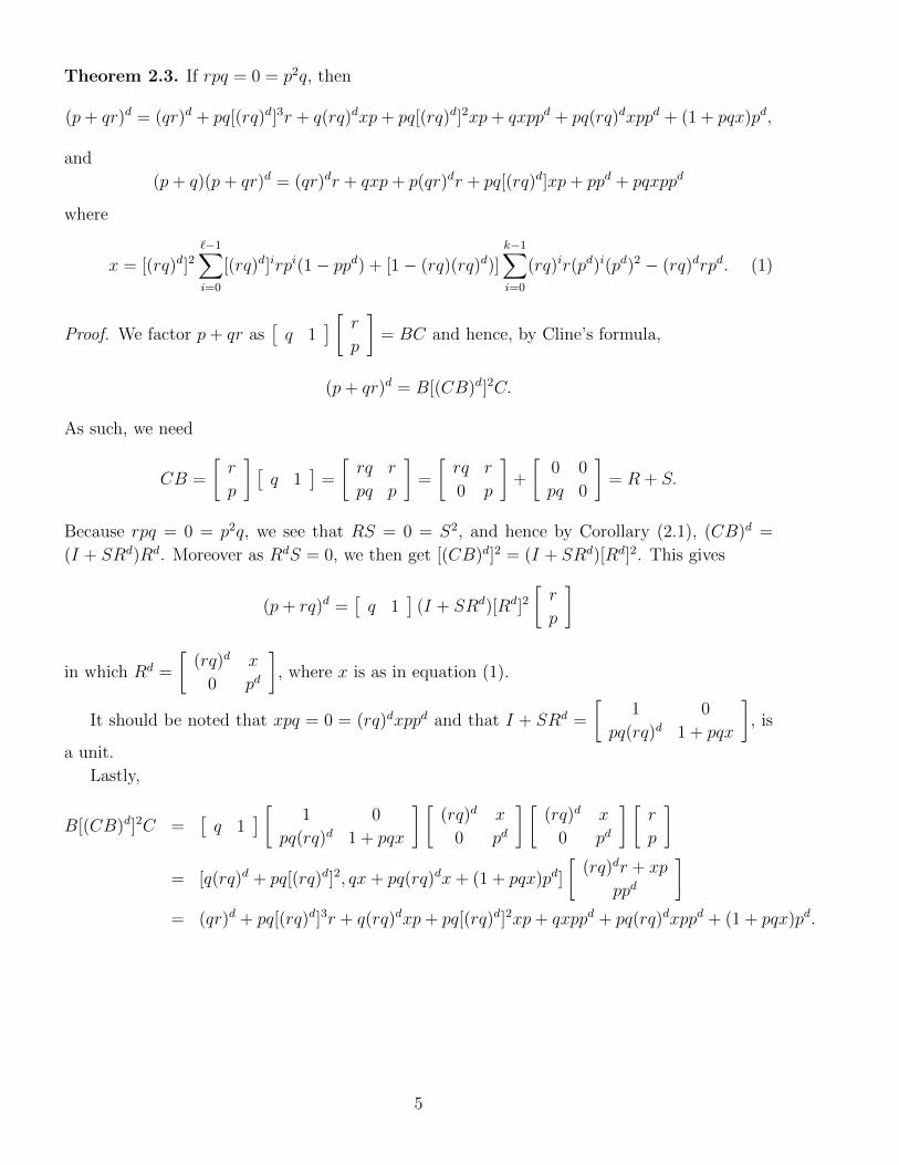
Theorem 2.3. If rpq = 0 = p2q, then
(p+ qr)d = (qr)d + pq[(rq)d]3r + q(rq)dxp+ pq[(rq)d]2xp+ qxppd + pq(rq)dxppd + (1 + pqx)pd,
and
(p+ q)(p+ qr)d = (qr)dr + qxp+ p(qr)dr + pq[(rq)d]xp+ ppd + pqxppd
where
x = [(rq)d]2`−1∑i=0
[(rq)d]irpi(1− ppd) + [1− (rq)(rq)d)]k−1∑i=0
(rq)ir(pd)i(pd)2 − (rq)drpd. (1)
Proof. We factor p+ qr as[q 1
] [ rp
]= BC and hence, by Cline’s formula,
(p+ qr)d = B[(CB)d]2C.
As such, we need
CB =
[r
p
] [q 1
]=
[rq r
pq p
]=
[rq r
0 p
]+
[0 0
pq 0
]= R + S.
Because rpq = 0 = p2q, we see that RS = 0 = S2, and hence by Corollary (2.1), (CB)d =
(I + SRd)Rd. Moreover as RdS = 0, we then get [(CB)d]2 = (I + SRd)[Rd]2. This gives
(p+ rq)d =[q 1
](I + SRd)[Rd]2
[r
p
]
in which Rd =
[(rq)d x
0 pd
], where x is as in equation (1).
It should be noted that xpq = 0 = (rq)dxppd and that I + SRd =
[1 0
pq(rq)d 1 + pqx
], is
a unit.
Lastly,
B[(CB)d]2C =[q 1
] [ 1 0
pq(rq)d 1 + pqx
] [(rq)d x
0 pd
] [(rq)d x
0 pd
] [r
p
]= [q(rq)d + pq[(rq)d]2, qx+ pq(rq)dx+ (1 + pqx)pd]
[(rq)dr + xp
ppd
]= (qr)d + pq[(rq)d]3r + q(rq)dxp+ pq[(rq)d]2xp+ qxppd + pq(rq)dxppd + (1 + pqx)pd.
5
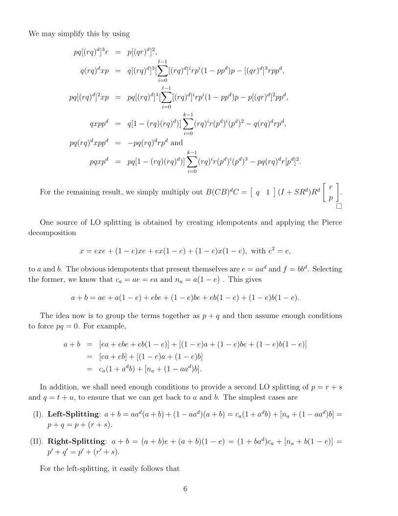
We may simplify this by using
pq[(rq)d]3r = p[(qr)d]2,
q(rq)dxp = q[(rq)d]3[`−1∑i=0
[(rq)d]irpi(1− ppd)p− [(qr)d]3rppd,
pq[(rq)d]2xp = pq[(rq)d]4[`−1∑i=0
[(rq)d]irpi(1− ppd)p− p[(qr)d]2ppd,
qxppd = q[1− (rq)(rq)d)]k−1∑i=0
(rq)ir(pd)i(pd)2 − q(rq)drpd,
pq(rq)dxppd = −pq(rq)drpd and
pqxpd = pq[1− (rq)(rq)d)]k−1∑i=0
(rq)ir(pd)i(pd)3 − pq(rq)dr[pd]2.
For the remaining result, we simply multiply out B(CB)dC =[q 1
](I + SRd)Rd
[r
p
].
One source of LO splitting is obtained by creating idempotents and applying the Pierce
decomposition
x = exe+ (1− e)xe+ ex(1− e) + (1− e)x(1− e), with e2 = e,
to a and b. The obvious idempotents that present themselves are e = aad and f = bbd. Selecting
the former, we know that ca = ae = ea and na = a(1− e) . This gives
a+ b = ae+ a(1− e) + ebe+ (1− e)be+ eb(1− e) + (1− e)b(1− e).
The idea now is to group the terms together as p + q and then assume enough conditions
to force pq = 0. For example,
a+ b = [ea+ ebe+ eb(1− e)] + [(1− e)a+ (1− e)be+ (1− e)b(1− e)]= [ea+ eb] + [(1− e)a+ (1− e)b]= ca(1 + adb) + [na + (1− aad)b].
In addition, we shall need enough conditions to provide a second LO splitting of p = r + s
and q = t+ u, to ensure that we can get back to a and b. The simplest cases are
(I). Left-Splitting: a+ b = aad(a+ b) + (1− aad)(a+ b) = ca(1 + adb) + [na + (1− aad)b] =
p+ q = p+ (r + s).
(II). Right-Splitting: a + b = (a + b)e + (a + b)(1 − e) = (1 + bad)ca + [na + b(1 − e)] =
p′ + q′ = p′ + (r′ + s).
For the left-splitting, it easily follows that
6

1. pq = qp if and only if pq = 0 = qp.
2. pq = 0 if and only if eb(1− e)(a+ b) = 0, in which case eb(1− e)be = 0.
3. qp = 0 if and only if (1− e)be(a+ b) = 0, in which case (1− e)beb(1− e) = 0.
Likewise, for the right-splitting we have
1. p′q′ = q′p′ if and only if p′q′ = 0 = q′p′.
2. q′p′ = 0 if and only if (a+ b)(1− e)be = 0, in which case eb(1− e)be = 0.
3. p′q′ = 0 if and only if (a+ b)eb(1− e) = 0, in which case (1− e)beb(1− e = 0.
Needless to say we may switch a and b to give a second formula.
Three especially simple cases occur when be = 0 or eb = 0. We begin with
Proposition 2.1. Let e = aad and f = bbd. If be = 0 then
(a+ b)d = (1− aad)pd + adk−1∑i=0
(ad)ipi(1− ppd) (2)
where p = a(1− e) + b .
Proof. We use the right-splitting,
a+ b = (a+ b)(1− e) + (a+ b)e = [a(1− e) + b] + ca = p+ q,
were pq = 0 and q# = ad. As such we have a LO splitting and, by Theorem (2.2),
(a+ b)d = (1− aad)pd + adk−1∑i=0
(ad)ipi(1− ppd).
It is clear that adp = adb, but (ad)2p2 cannot be simplified. We now must impose sufficient
conditions on a and b so that we can split p as well.
We require the following preliminary fact:
Lemma 2.2. 1. If be = 0 then (1−e)ab = (1−e)ba if and only if na commutes with (1−e)b.
2. If eb = 0 then ab(1− e) = ba(1− e) if and only if na commutes with b(1− e).
Proof. (1). (1− e)bna = (1− e)b(1− e)a = (1− e)ba and na(1− e)b = nab = (1− e)ab.(2). By symmetry b(1−e)na = bna = ba(1−e) and nab(1−e) = a(1−e)b(1−e) = ab(1−e).
We are now ready for
Proposition 2.2. Let e = aad and f = bbd.
7
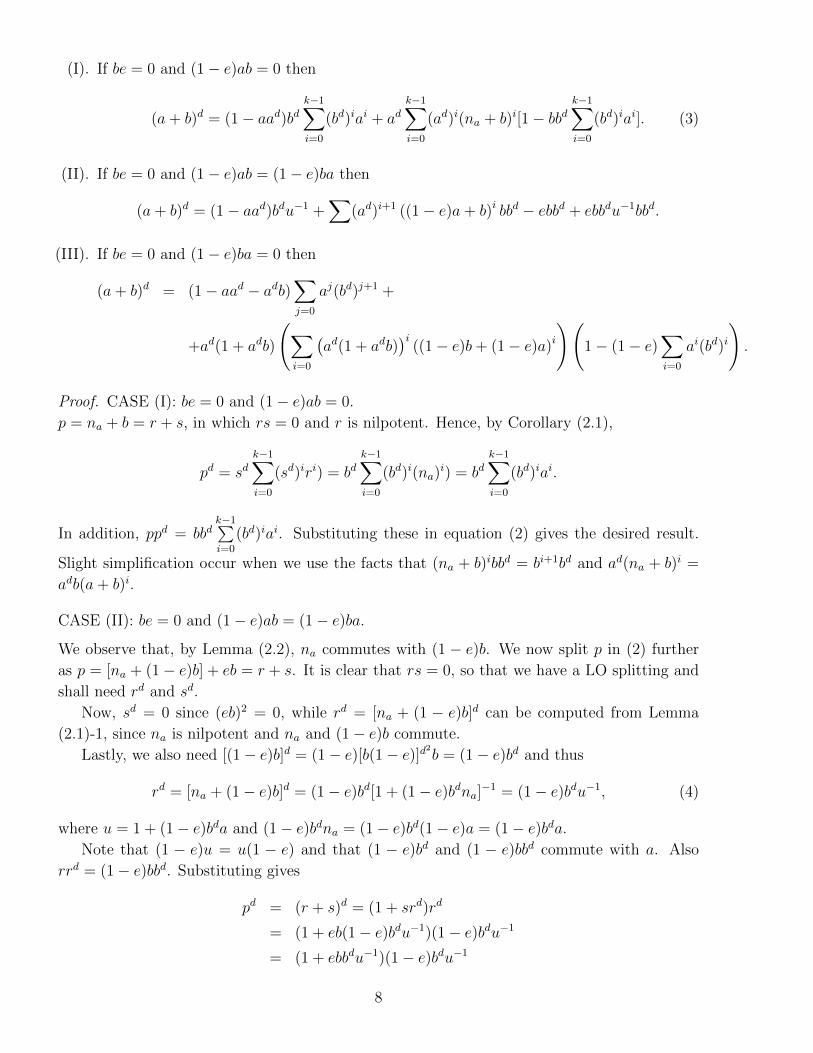
(I). If be = 0 and (1− e)ab = 0 then
(a+ b)d = (1− aad)bdk−1∑i=0
(bd)iai + adk−1∑i=0
(ad)i(na + b)i[1− bbdk−1∑i=0
(bd)iai]. (3)
(II). If be = 0 and (1− e)ab = (1− e)ba then
(a+ b)d = (1− aad)bdu−1 +∑
(ad)i+1 ((1− e)a+ b)i bbd − ebbd + ebbdu−1bbd.
(III). If be = 0 and (1− e)ba = 0 then
(a+ b)d = (1− aad − adb)∑j=0
aj(bd)j+1 +
+ad(1 + adb)
(∑i=0
(ad(1 + adb)
)i((1− e)b+ (1− e)a)i
)(1− (1− e)
∑i=0
ai(bd)i
).
Proof. CASE (I): be = 0 and (1− e)ab = 0.
p = na + b = r + s, in which rs = 0 and r is nilpotent. Hence, by Corollary (2.1),
pd = sdk−1∑i=0
(sd)iri) = bdk−1∑i=0
(bd)i(na)i) = bd
k−1∑i=0
(bd)iai.
In addition, ppd = bbdk−1∑i=0
(bd)iai. Substituting these in equation (2) gives the desired result.
Slight simplification occur when we use the facts that (na + b)ibbd = bi+1bd and ad(na + b)i =
adb(a+ b)i.
CASE (II): be = 0 and (1− e)ab = (1− e)ba.
We observe that, by Lemma (2.2), na commutes with (1 − e)b. We now split p in (2) further
as p = [na + (1− e)b] + eb = r + s. It is clear that rs = 0, so that we have a LO splitting and
shall need rd and sd.
Now, sd = 0 since (eb)2 = 0, while rd = [na + (1 − e)b]d can be computed from Lemma
(2.1)-1, since na is nilpotent and na and (1− e)b commute.
Lastly, we also need [(1− e)b]d = (1− e)[b(1− e)]d2b = (1− e)bd and thus
rd = [na + (1− e)b]d = (1− e)bd[1 + (1− e)bdna]−1 = (1− e)bdu−1, (4)
where u = 1 + (1− e)bda and (1− e)bdna = (1− e)bd(1− e)a = (1− e)bda.
Note that (1 − e)u = u(1 − e) and that (1 − e)bd and (1 − e)bbd commute with a. Also
rrd = (1− e)bbd. Substituting gives
pd = (r + s)d = (1 + srd)rd
= (1 + eb(1− e)bdu−1)(1− e)bdu−1
= (1 + ebbdu−1)(1− e)bdu−1
8

and
ppd = (1 + srd)rrd
= (1 + eb(1− e)bdu−1)(1− e)bbd
= (1 + ebbdu−1)(1− e)bbd
= bbd − ebbd + ebbdu−1bbd = bbd + eX.
We then arrive at
(a+ b)d = (1− aad)[1 + ebbdu−1](1− e)bdu−1 + ad[k−1∑i=0
(ad)i(na + b)i(1− bbd)]. (5)
Case (III): be = 0 and (1− e)ba = 0.
We now use a different splitting
a+ b = (1− e)(a+ b) + e(a+ b) = p+ q,
where pq = 0. Now p = r+ s where r = (1− e)b and s = a(1− e). Thus rs = 0, s is nilpotent,
rd = [(1− e)b]d = (1− e)bd and rrd = (1− e)bbd. Hence by Corollary (2.1), we see that
pd = (r + s)d =k−1∑i=0
si(rd)ird =k−1∑i=0
(na)i[(1− e)b)]d)i+1 = (1− e)Wbd
where W =k−1∑i=0
ai(bd)i and
ppd =k−1∑i=0
si(rd)irrd = (1− e)k−1∑i=0
ai(bd)i+1(1− e)b = (1− e)W.
Next we observe that q = eb + ae = t + u, where tu = 0 = t2. Again by Corollary (2.1) we
get qd = ud(1 + udt) = ad(1 + adb) and qqd = uud(1 + udt) = aad(1 + adb)
Lastly, we substitute the expressions for pd, ppd, qd and qqd in Theorem (2.2) and obtain
(a+ b)d = (1− qqd)
(∑i=0
qi(pd)i
)pd + qd
(∑i=0
(qd)ipi
)(1− ppd)
= (1− aad − adb)∑i=0
[e(a+ b)]i[(1− e)Wbd]i+1 +
+ad(1 + adb)∑i=0
[ad(1 + adb)]i[(1− e)(a+ b)]i[1− (1− e)W ].
Since (e(a+ b))i = eai−1(b+ a), for all i ≥ 1, and also (1− aad − adb)e = 0, we see that
(1− aad − adb)
(∑i=1
[e(a+ b)]i((1− e)Wbd
)i+1
)= 0
9
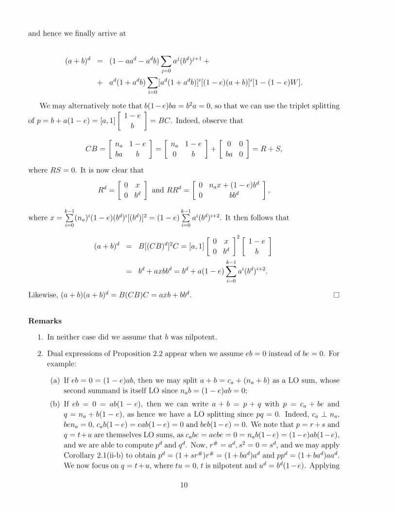
and hence we finally arrive at
(a+ b)d = (1− aad − adb)∑j=0
aj(bd)j+1 +
+ ad(1 + adb)∑i=0
[ad(1 + adb)]i[(1− e)(a+ b)]i[1− (1− e)W ].
We may alternatively note that b(1−e)ba = b2a = 0, so that we can use the triplet splitting
of p = b+ a(1− e) = [a, 1]
[1− eb
]= BC. Indeed, observe that
CB =
[na 1− eba b
]=
[na 1− e0 b
]+
[0 0
ba 0
]= R + S,
where RS = 0. It is now clear that
Rd =
[0 x
0 bd
]and RRd =
[0 nax+ (1− e)bd0 bbd
],
where x =k−1∑i=0
(na)i(1− e)(bd)i[(bd)]2 = (1− e)
k−1∑i=0
ai(bd)i+2. It then follows that
(a+ b)d = B[(CB)d]2C = [a, 1]
[0 x
0 bd
]2 [1− eb
]= bd + axbbd = bd + a(1− e)
k−1∑i=0
ai(bd)i+2.
Likewise, (a+ b)(a+ b)d = B(CB)C = axb+ bbd.
Remarks
1. In neither case did we assume that b was nilpotent.
2. Dual expressions of Proposition 2.2 appear when we assume eb = 0 instead of be = 0. For
example:
(a) If eb = 0 = (1 − e)ab, then we may split a + b = ca + (na + b) as a LO sum, whose
second summand is itself LO since nab = (1− e)ab = 0;
(b) If eb = 0 = ab(1 − e), then we can write a + b = p + q with p = ca + be and
q = na + b(1 − e), as hence we have a LO splitting since pq = 0. Indeed, ca ⊥ na,
bena = 0, cab(1− e) = eab(1− e) = 0 and beb(1− e) = 0. We note that p = r+s and
q = t+u are themselves LO sums, as cabe = aebe = 0 = nab(1−e) = (1−e)ab(1−e),and we are able to compute pd and qd. Now, r# = ad, s2 = 0 = sd, and we may apply
Corollary 2.1(ii-b) to obtain pd = (1 + sr#)r# = (1 + bad)ad and ppd = (1 + bad)aad.
We now focus on q = t+u, where tu = 0, t is nilpotent and ud = bd(1−e). Applying
10

Corollary 2.1(i-a), and since (bd(1−e))i = (bd)i(1−e), we obtain qd = ud[∑
(ud)iti] =
bd(1− e)∑
(bd)i[(1− e)a]i and qqd = bbd(1− e)∑
(bd)i[(1− e)a]i. Theorem 2.2 allows
us, now, to compute the D-inverse of p+ q = a+ b.
(c) If eb = 0 and (1 − e)ab = (1 − e)ba then na and b(1 − e) commute. Taking p = caand q = na + b, then a + b = p + q, with pq = 0 and p# exists. We split q
further as q = be + (na + b(1 − e)) = r + s, with rs = 0, sd = bd(1 − e)w−1,
ssd = bbd(1 − e), r2 = 0 = rd, where w = 1 + bd(1 − e)a. Therefore, p# = ad,
qd = sd(1+sdr) = bd(1−e)w−1(1+bd(1−e)w−1be), qqd = ssd(1+sdr) = bbd(1−e)w−1,which gives
(a+ b)d = (1− bbd(1− e)w−1)[∑
(na + b)i(ad)i]ad + bd(1− e)w−1(1− e).
3 Inclusions
Consider the matrix M =
[a 1
b 0
], where ad and bd exist, and set f = bbd and nb = b(1− bbd).
We shall show below that in the following list each of the special cases implies the next.
Moreover we shall show that finding the D-inverse for the “most general” case (7) uses the
computation of the D-inverse for the “simplest” case (1). As such we can say that all cases are
really “equivalent”.
1. a = 1, b = n is nilpotent
2. a = 1
3. ab = ba and a is a unit
4. adb = bad and baad = b
5. ab = ba
6. af = fa and anb = nba
7. af = faf and anb = nba
It is also clear that the last conditions automatically hold if b is invertible, when M is
invertible, or when b is nilpotent and ab = ba. We shall compute Md for the latter case, which
in turn however, makes use of the first case. The chain of implications is supported by the
following result.
Lemma 3.1. (i) If ab = bc then adb = bcd (but not conversely).
(ii) If adb = bcd, then aadb = bccd (but not conversely).
(iii) If A is a square matrix over a field then Ad is a polynomial in A.
11
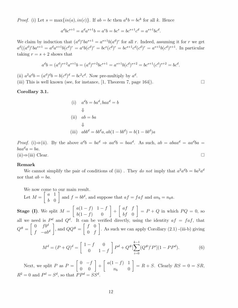
Proof. (i) Let s = max{in(a), in(c)}. If ab = bc then akb = bck for all k. Hence
adbcs+1 = adas+1b = asb = bcs = bcs+1cd = as+1bcd.
We claim by induction that (ad)rbas+1 = as+1b(ad)r for all r. Indeed, assuming it for r we get
ad((ad)rbas+1 = adas+1b(cd)r = asb(cd)r = bcs(cd)r = bcs+1cd(cd)r = as+1b(cd)s+1. In particular
taking r = s+ 2 shows that
adb = (ad)s+2as+1b = (ad)s+2bcs+1 = as+1b(cd)s+2 = bcs+1(cd)s+2 = bcd.
(ii) a2adb = (ad)db = b(cd)d = bc2cd. Now pre-multiply by ad.
(iii) This is well known (see, for instance, [1, Theorem 7, page 164]).
Corollary 3.1.
(i) adb = bad, baad = b
⇓(ii) ab = ba
⇓(iii) abbd = bbda, ab(1− bbd) = b(1− bbd)a
Proof. (i)⇒(ii). By the above adb = bad ⇒ aadb = baad. As such, ab = abaad = aadba =
baada = ba.
(ii)⇒(iii) Clear.
Remark
We cannot simplify the pair of conditions of (iii) . They do not imply that a2adb = ba2ad
nor that ab = ba.
We now come to our main result.
Let M =
[a 1
b 0
]and f = bbd, and suppose that af = faf and anb = nba.
Stage (I). We split M =
[a(1− f) 1− fb(1− f) 0
]+
[af f
bf 0
]= P + Q in which PQ = 0, so
all we need is P d and Qd. It can be verified directly, using the identity af = faf , that
Q# =
[0 fbd
f −abd
], and QQ# =
[f 0
0 f
]. As such we can apply Corollary (2.1) -(iii-b) giving
Md = (P +Q)d =
[1− f 0
0 1− f
]P d +Q#[
k−1∑i=0
(Q#)iP i](1− PP d). (6)
Next, we split P as P =
[0 −f0 0
]+
[a(1− f) 1
nb 0
]= R + S. Clearly RS = 0 = SR,
R2 = 0 and P d = Sd, so that PP d = SSd.
12
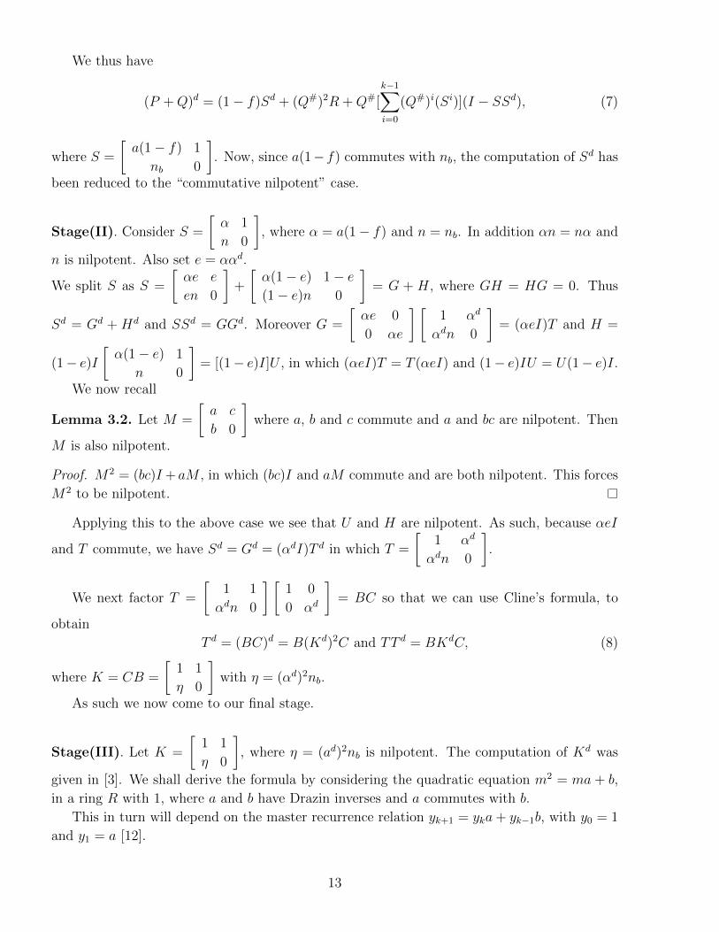
We thus have
(P +Q)d = (1− f)Sd + (Q#)2R +Q#[k−1∑i=0
(Q#)i(Si)](I − SSd), (7)
where S =
[a(1− f) 1
nb 0
]. Now, since a(1− f) commutes with nb, the computation of Sd has
been reduced to the “commutative nilpotent” case.
Stage(II). Consider S =
[α 1
n 0
], where α = a(1− f) and n = nb. In addition αn = nα and
n is nilpotent. Also set e = ααd.
We split S as S =
[αe e
en 0
]+
[α(1− e) 1− e(1− e)n 0
]= G + H, where GH = HG = 0. Thus
Sd = Gd + Hd and SSd = GGd. Moreover G =
[αe 0
0 αe
] [1 αd
αdn 0
]= (αeI)T and H =
(1− e)I[α(1− e) 1
n 0
]= [(1− e)I]U , in which (αeI)T = T (αeI) and (1− e)IU = U(1− e)I.
We now recall
Lemma 3.2. Let M =
[a c
b 0
]where a, b and c commute and a and bc are nilpotent. Then
M is also nilpotent.
Proof. M2 = (bc)I + aM , in which (bc)I and aM commute and are both nilpotent. This forces
M2 to be nilpotent.
Applying this to the above case we see that U and H are nilpotent. As such, because αeI
and T commute, we have Sd = Gd = (αdI)T d in which T =
[1 αd
αdn 0
].
We next factor T =
[1 1
αdn 0
] [1 0
0 αd
]= BC so that we can use Cline’s formula, to
obtain
T d = (BC)d = B(Kd)2C and TT d = BKdC, (8)
where K = CB =
[1 1
η 0
]with η = (αd)2nb.
As such we now come to our final stage.
Stage(III). Let K =
[1 1
η 0
], where η = (ad)2nb is nilpotent. The computation of Kd was
given in [3]. We shall derive the formula by considering the quadratic equation m2 = ma + b,
in a ring R with 1, where a and b have Drazin inverses and a commutes with b.
This in turn will depend on the master recurrence relation yk+1 = yka+ yk−1b, with y0 = 1
and y1 = a [12].
13
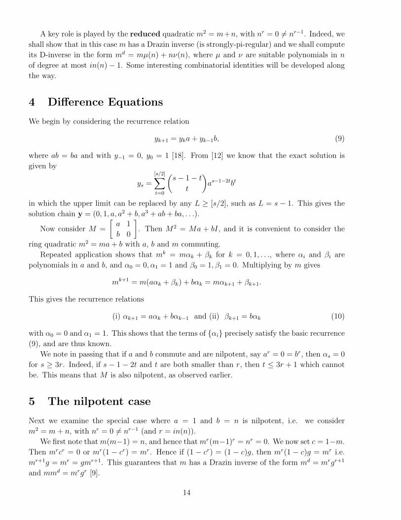
A key role is played by the reduced quadratic m2 = m+n, with nr = 0 6= nr−1. Indeed, we
shall show that in this case m has a Drazin inverse (is strongly-pi-regular) and we shall compute
its D-inverse in the form md = mµ(n) + nν(n), where µ and ν are suitable polynomials in n
of degree at most in(n)− 1. Some interesting combinatorial identities will be developed along
the way.
4 Difference Equations
We begin by considering the recurrence relation
yk+1 = yka+ yk−1b, (9)
where ab = ba and with y−1 = 0, y0 = 1 [18]. From [12] we know that the exact solution is
given by
ys =
[s/2]∑t=0
(s− 1− t
t
)as−1−2tbt
in which the upper limit can be replaced by any L ≥ [s/2], such as L = s − 1. This gives the
solution chain y = (0, 1, a, a2 + b, a3 + ab+ ba, . . .).
Now consider M =
[a 1
b 0
]. Then M2 = Ma + bI, and it is convenient to consider the
ring quadratic m2 = ma+ b with a, b and m commuting.
Repeated application shows that mk = mαk + βk for k = 0, 1, . . ., where αi and βi are
polynomials in a and b, and α0 = 0, α1 = 1 and β0 = 1, β1 = 0. Multiplying by m gives
mk+1 = m(aαk + βk) + bαk = mαk+1 + βk+1.
This gives the recurrence relations
(i) αk+1 = aαk + bαk−1 and (ii) βk+1 = bαk (10)
with α0 = 0 and α1 = 1. This shows that the terms of {αi} precisely satisfy the basic recurrence
(9), and are thus known.
We note in passing that if a and b commute and are nilpotent, say ar = 0 = br, then αs = 0
for s ≥ 3r. Indeed, if s − 1 − 2t and t are both smaller than r, then t ≤ 3r + 1 which cannot
be. This means that M is also nilpotent, as observed earlier.
5 The nilpotent case
Next we examine the special case where a = 1 and b = n is nilpotent, i.e. we consider
m2 = m+ n, with nr = 0 6= nr−1 (and r = in(n)).
We first note that m(m−1) = n, and hence that mr(m−1)r = nr = 0. We now set c = 1−m.
Then mrcr = 0 or mr(1 − cr) = mr. Hence if (1 − cr) = (1 − c)g, then mr(1 − c)g = mr i.e.
mr+1g = mr = gmr+1. This guarantees that m has a Drazin inverse of the form md = mrgr+1
and mmd = mrgr [9].
14
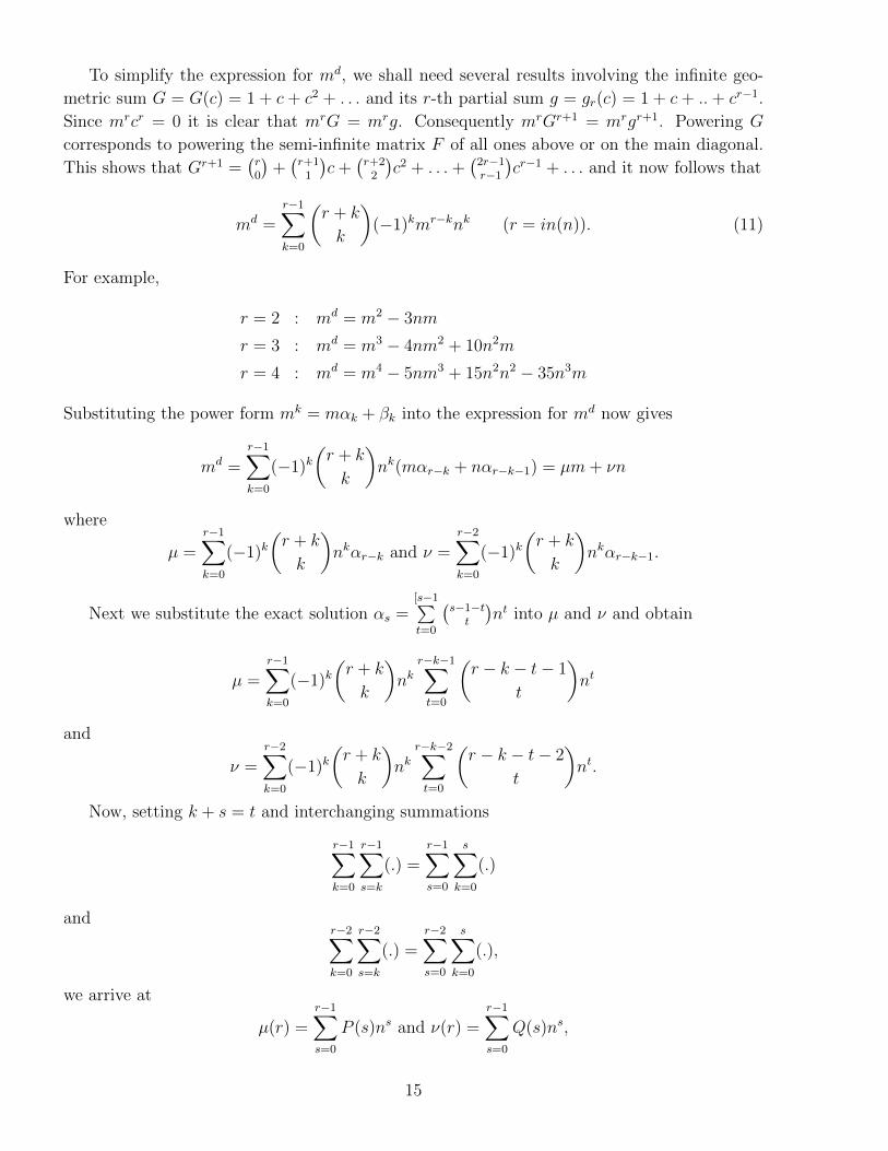
To simplify the expression for md, we shall need several results involving the infinite geo-
metric sum G = G(c) = 1 + c + c2 + . . . and its r-th partial sum g = gr(c) = 1 + c + .. + cr−1.
Since mrcr = 0 it is clear that mrG = mrg. Consequently mrGr+1 = mrgr+1. Powering G
corresponds to powering the semi-infinite matrix F of all ones above or on the main diagonal.
This shows that Gr+1 =(r0
)+(r+11
)c+
(r+22
)c2 + . . .+
(2r−1r−1
)cr−1 + . . . and it now follows that
md =r−1∑k=0
(r + k
k
)(−1)kmr−knk (r = in(n)). (11)
For example,
r = 2 : md = m2 − 3nm
r = 3 : md = m3 − 4nm2 + 10n2m
r = 4 : md = m4 − 5nm3 + 15n2n2 − 35n3m
Substituting the power form mk = mαk + βk into the expression for md now gives
md =r−1∑k=0
(−1)k(r + k
k
)nk(mαr−k + nαr−k−1) = µm+ νn
where
µ =r−1∑k=0
(−1)k(r + k
k
)nkαr−k and ν =
r−2∑k=0
(−1)k(r + k
k
)nkαr−k−1.
Next we substitute the exact solution αs =[s−1∑t=0
(s−1−tt
)nt into µ and ν and obtain
µ =r−1∑k=0
(−1)k(r + k
k
)nk
r−k−1∑t=0
(r − k − t− 1
t
)nt
and
ν =r−2∑k=0
(−1)k(r + k
k
)nk
r−k−2∑t=0
(r − k − t− 2
t
)nt.
Now, setting k + s = t and interchanging summations
r−1∑k=0
r−1∑s=k
(.) =r−1∑s=0
s∑k=0
(.)
andr−2∑k=0
r−2∑s=k
(.) =r−2∑s=0
s∑k=0
(.),
we arrive at
µ(r) =r−1∑s=0
P (s)ns and ν(r) =r−1∑s=0
Q(s)ns,
15
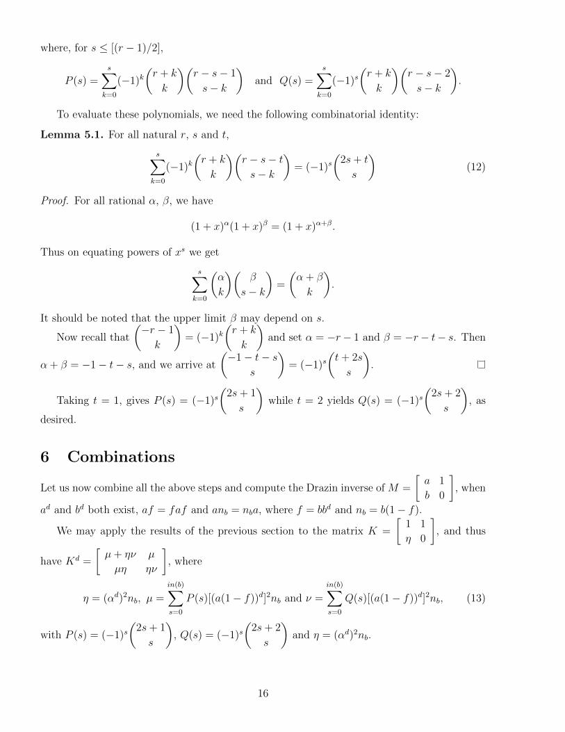
where, for s ≤ [(r − 1)/2],
P (s) =s∑
k=0
(−1)k(r + k
k
)(r − s− 1
s− k
)and Q(s) =
s∑k=0
(−1)s(r + k
k
)(r − s− 2
s− k
).
To evaluate these polynomials, we need the following combinatorial identity:
Lemma 5.1. For all natural r, s and t,
s∑k=0
(−1)k(r + k
k
)(r − s− ts− k
)= (−1)s
(2s+ t
s
)(12)
Proof. For all rational α, β, we have
(1 + x)α(1 + x)β = (1 + x)α+β.
Thus on equating powers of xs we get
s∑k=0
(α
k
)(β
s− k
)=
(α + β
k
).
It should be noted that the upper limit β may depend on s.
Now recall that
(−r − 1
k
)= (−1)k
(r + k
k
)and set α = −r− 1 and β = −r− t− s. Then
α + β = −1− t− s, and we arrive at
(−1− t− s
s
)= (−1)s
(t+ 2s
s
).
Taking t = 1, gives P (s) = (−1)s(
2s+ 1
s
)while t = 2 yields Q(s) = (−1)s
(2s+ 2
s
), as
desired.
6 Combinations
Let us now combine all the above steps and compute the Drazin inverse of M =
[a 1
b 0
], when
ad and bd both exist, af = faf and anb = nba, where f = bbd and nb = b(1− f).
We may apply the results of the previous section to the matrix K =
[1 1
η 0
], and thus
have Kd =
[µ+ ην µ
µη ην
], where
η = (αd)2nb, µ =
in(b)∑s=0
P (s)[(a(1− f))d]2nb and ν =
in(b)∑s=0
Q(s)[(a(1− f))d]2nb, (13)
with P (s) = (−1)s(
2s+ 1
s
), Q(s) = (−1)s
(2s+ 2
s
)and η = (αd)2nb.
16
From equation (8), TT d =
[1 1
αdnb 0
]Kd
[1 0
0 αd
]and T d =
[1 1
αdnb 0
] (Kd)2 [ 1 0
0 αd
],
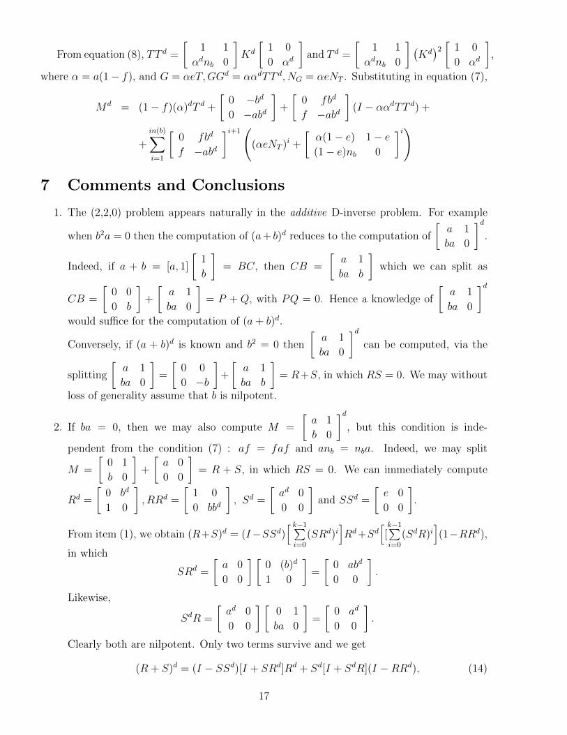
where α = a(1− f), and G = αeT,GGd = ααdTT d, NG = αeNT . Substituting in equation (7),
Md = (1− f)(α)dT d +
[0 −bd0 −abd
]+
[0 fbd
f −abd
](I − ααdTT d) +
+
in(b)∑i=1
[0 fbd
f −abd
]i+1(
(αeNT )i +
[α(1− e) 1− e(1− e)nb 0
]i)
7 Comments and Conclusions
1. The (2,2,0) problem appears naturally in the additive D-inverse problem. For example
when b2a = 0 then the computation of (a+ b)d reduces to the computation of
[a 1
ba 0
]d.
Indeed, if a + b = [a, 1]
[1
b
]= BC, then CB =
[a 1
ba b
]which we can split as
CB =
[0 0
0 b
]+
[a 1
ba 0
]= P + Q, with PQ = 0. Hence a knowledge of
[a 1
ba 0
]dwould suffice for the computation of (a+ b)d.
Conversely, if (a + b)d is known and b2 = 0 then
[a 1
ba 0
]dcan be computed, via the
splitting
[a 1
ba 0
]=
[0 0
0 −b
]+
[a 1
ba b
]= R+S, in which RS = 0. We may without
loss of generality assume that b is nilpotent.
2. If ba = 0, then we may also compute M =
[a 1
b 0
]d, but this condition is inde-
pendent from the condition (7) : af = faf and anb = nba. Indeed, we may split
M =
[0 1
b 0
]+
[a 0
0 0
]= R + S, in which RS = 0. We can immediately compute
Rd =
[0 bd
1 0
], RRd =
[1 0
0 bbd
], Sd =
[ad 0
0 0
]and SSd =
[e 0
0 0
].
From item (1), we obtain (R+S)d = (I−SSd)[ k−1∑i=0
(SRd)i]Rd+Sd
[[k−1∑i=0
(SdR)i](1−RRd),
in which
SRd =
[a 0
0 0
] [0 (b)d
1 0
]=
[0 abd
0 0
].
Likewise,
SdR =
[ad 0
0 0
] [0 1
ba 0
]=
[0 ad
0 0
].
Clearly both are nilpotent. Only two terms survive and we get
(R + S)d = (I − SSd)[I + SRd]Rd + Sd[I + SdR](I −RRd), (14)
17
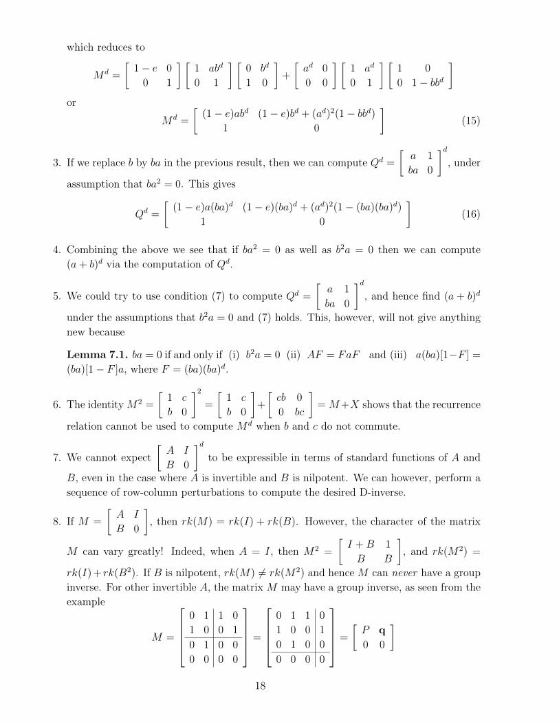
which reduces to
Md =
[1− e 0
0 1
] [1 abd
0 1
] [0 bd
1 0
]+
[ad 0
0 0
] [1 ad
0 1
] [1 0
0 1− bbd
]or
Md =
[(1− e)abd (1− e)bd + (ad)2(1− bbd)
1 0
](15)
3. If we replace b by ba in the previous result, then we can compute Qd =
[a 1
ba 0
]d, under
assumption that ba2 = 0. This gives
Qd =
[(1− e)a(ba)d (1− e)(ba)d + (ad)2(1− (ba)(ba)d)
1 0
](16)
4. Combining the above we see that if ba2 = 0 as well as b2a = 0 then we can compute
(a+ b)d via the computation of Qd.
5. We could try to use condition (7) to compute Qd =
[a 1
ba 0
]d, and hence find (a + b)d
under the assumptions that b2a = 0 and (7) holds. This, however, will not give anything
new because
Lemma 7.1. ba = 0 if and only if (i) b2a = 0 (ii) AF = FaF and (iii) a(ba)[1−F ] =
(ba)[1− F ]a, where F = (ba)(ba)d.
6. The identity M2 =
[1 c
b 0
]2=
[1 c
b 0
]+
[cb 0
0 bc
]= M+X shows that the recurrence
relation cannot be used to compute Md when b and c do not commute.
7. We cannot expect
[A I
B 0
]dto be expressible in terms of standard functions of A and
B, even in the case where A is invertible and B is nilpotent. We can however, perform a
sequence of row-column perturbations to compute the desired D-inverse.
8. If M =
[A I
B 0
], then rk(M) = rk(I) + rk(B). However, the character of the matrix
M can vary greatly! Indeed, when A = I, then M2 =
[I +B 1
B B
], and rk(M2) =
rk(I) + rk(B2). If B is nilpotent, rk(M) 6= rk(M2) and hence M can never have a group
inverse. For other invertible A, the matrix M may have a group inverse, as seen from the
example
M =
0 1 1 0
1 0 0 1
0 1 0 0
0 0 0 0
=
0 1 1 0
1 0 0 1
0 1 0 0
0 0 0 0
=
[P q
0 0
]
18
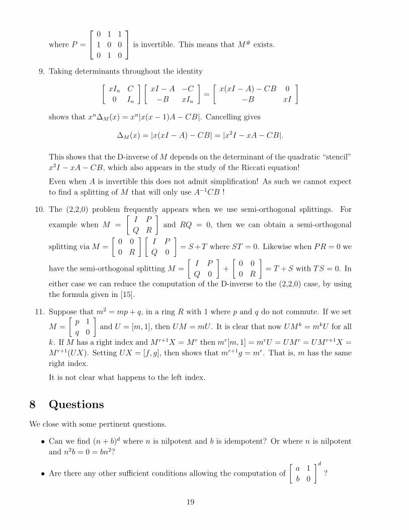
where P =
0 1 1
1 0 0
0 1 0
is invertible. This means that M# exists.
9. Taking determinants throughout the identity[xIn C
0 In
] [xI − A −C−B xIn
]=
[x(xI − A)− CB 0
−B xI
]shows that xn∆M(x) = xn|x(x− 1)A− CB|. Cancelling gives
∆M(x) = |x(xI − A)− CB| = |x2I − xA− CB|.
This shows that the D-inverse of M depends on the determinant of the quadratic “stencil”
x2I − xA− CB, which also appears in the study of the Riccati equation!
Even when A is invertible this does not admit simplification! As such we cannot expect
to find a splitting of M that will only use A−1CB !
10. The (2,2,0) problem frequently appears when we use semi-orthogonal splittings. For
example when M =
[I P
Q R
]and RQ = 0, then we can obtain a semi-orthogonal
splitting via M =
[0 0
0 R
] [I P
Q 0
]= S+T where ST = 0. Likewise when PR = 0 we
have the semi-orthogonal splitting M =
[I P
Q 0
]+
[0 0
0 R
]= T +S with TS = 0. In
either case we can reduce the computation of the D-inverse to the (2,2,0) case, by using
the formula given in [15].
11. Suppose that m2 = mp+ q, in a ring R with 1 where p and q do not commute. If we set
M =
[p 1
q 0
]and U = [m, 1], then UM = mU . It is clear that now UMk = mkU for all
k. If M has a right index and M r+1X = M r then mr[m, 1] = mrU = UM r = UM r+1X =
M r+1(UX). Setting UX = [f, g], then shows that mr+1g = mr. That is, m has the same
right index.
It is not clear what happens to the left index.
8 Questions
We close with some pertinent questions.
• Can we find (n + b)d where n is nilpotent and b is idempotent? Or where n is nilpotent
and n2b = 0 = bn2?
• Are there any other sufficient conditions allowing the computation of
[a 1
b 0
]d?
19
Acknowledgment
This research was financed by FEDER Funds through “Programa Operacional Factores de
Competitividade – COMPETE” and by Portuguese Funds through FCT - “Fundacao para a
Ciencia e a Tecnologia”, within the project PEst-C/MAT/UI0013/2011.
References
[1] Ben Israel, A.; Greville, T. N. E.; Generalized Inverses, Theory and Applications, 2nd
Edition, Springer, New York 2003.
[2] C. Bu, J. Zhao and J. Zheng, Group inverse for a class of 2× 2 block matrices over skew
fields, Applied Math. Comp. 204, (2008) 45–49.
[3] N. Castro-Gonzalez and E. Dopazo, Representations of the Drazin inverse for a class of
block matrices, Linear Algebra Appl. 400 (2005), 253–269.
[4] N. Castro-Gonzalez, E. Dopazo and J. Robles, Formulas for the Drazin Inverse of special
block matrices, Appl. Math. Comput. 174 (2006), no. 1, 252–270.
[5] N. Castro-Gonzalez, E. Dopazo and M. F. Martınez-Serrano, On the Drazin inverse of the
sum of two operators and its application to operator matrices, J. Math. Anal. Appl. 350
(2009), no. 1, 207–215.
[6] N. Castro-Gonzalez and R. E. Hartwig, Companion Matrices and Linear Recurrences,
submitted.
[7] R.E. Cline, An application of representation of a matrix, MRC Technical Report, 592, 1965.
[8] C. Deng and Y. Wei, A note on the Drazin inverse of an anti-triangular matrix, Linear
Algebra Appl. 431 (2009), no. 10, 1910–1922.
[9] M. P. Drazin, Pseudo-inverses in associative rings and semigroups, Amer. Math. Monthly
65 (1958), 506–514.
[10] R. E. Hartwig, More on the Souriau-Frame algorithm and the Drazin inverse, SIAM J.
Appl. Math. 31 (1976), no. 1, 42–46.
[11] R. E. Hartwig, Theory and applications of matrix perturbations, with respect to Hankel
matrices and power formulæ, Internat. J. Systems Sci. 10 (1979), no. 4, 437–460.
[12] R. E. Hartwig, Note on a linear difference equation, Amer. Math. Monthly 113 (2006),
no. 3, 250–256.
[13] R. E. Hartwig, Block Generalized Inverses, Arch. Rat. Mech. Anal. 61 (1976), 197–251.
[14] R. E. Hartwig and J. Shoaf, Group inverses and Drazin inverses of bidiagonal and triangular
Toeplitz matrices, J. Austral. Math. Soc. Ser. A 24 (1977), no. 1, 10–34.
20
[15] R. E. Hartwig, Y.Wei and G. Wang, Some additive results on Drazin inverse, Linear
Algebra Appl. 322 (2001), no. 1-3, 207–217.
[16] X. Li and Y. Wei, A note on the representations for the Drazin inverse of 2 × 2 block
matrices, Linear Algebra Appl. 423 (2007), no. 2-3, 332–338.
[17] P. Patrıcio and R. E. Hartwig, Some additive results on Drazin inverses, Appl. Math.
Comput. 215 (2009), no. 2, 530–538.
[18] H. Siebeck, Die recurrenten Reihen vom Standpunkte der Zahlentheorie aus betrachtet,
Journal fur die reine und angewandte Mathematik, (1846), 71–77.
21
Related Documents