Th eE ffect of Stabilization in Finite Element Methods fo rt he Optimal Boundary Control of the Oseen Equations

The Effect of Stabilization in Finite Element Methodsfor the Optimal Boundary Control of the Oseen Equations ∗

Feby AbrahamDepartment of Mechanical Engineering and Materials Science

Rice University - MS 321, 6100 Main StreetHouston, TX 77005, USA

[email protected]

Marek Behr†

Lehrstuhl fur Numerische MechanikTechnische Universitat Munchen, Boltzmannstr. 15

D-85747 Garching, [email protected]

Matthias HeinkenschlossDepartment of Computational and Applied Mathematics

Rice University - MS 134, 6100 Main StreetHouston, TX 77005, [email protected]

Revised: May 7, 2004

Abstract

We study the effect of the Galerkin/Least-Squares (GLS) stabilization on the finite element discretiza-tion of optimal control problems governed by the linear Oseen equations. Control is applied in the formof suction or blowing on part of the boundary. Two ways of including the GLS stabilization into thediscretization of the optimal control problem are discussed. In one case the optimal control problem isfirst discretized and the resulting finite dimensional problem is then solved. In the other case, the op-timality conditions are first formulated on the differential equation level and are then discretized. Bothapproaches lead to different discrete adjoint equations and, depending on the choice of the stabilizationparameters and grid size, may significantly affect the computed control. The effect of the order in whichthe discretization is applied and the choice of the stabilization parameters are illustrated using two testproblems. The cause of the differences in the computed controls are explored numerically. Diagnosticsare introduced that may guide the selection of sensible stabilization parameters.

Keywords: Optimal boundary control, stabilized finite element methods, Oseen equations, solutionaccuracy.

1. Introduction

Stabilized finite element methods (FEMs) are frequently and successfully used to discretize advection-dominated partial differential equations (PDEs) [1], or to circumvent the compatibility conditions restricting

∗The authors gratefully acknowledge computing resources made available by the National Partnership for Advanced Com-putational Infrastructure (NPACI). Additional computing resources were provided by the NSF MRI award EIA-0116289. Thiswork was supported by the National Science Foundation under award ACI-0121360, CTS-ITR-0312764, and by Texas ATP grant003604-0011-2001.

†Corresponding author.

1

the choice of interpolation function spaces [2]. One question that arises in the application of these methodsis the choice of the stabilization parameter. For many PDE model problems this issue has been studied ana-lytically and numerically [3, 4]. However, the impact on the choice of the stabilization parameter when thestabilized FEM is used in the context of optimal control is not well studied. It is not true that a scheme whichgives good approximations to the PDE solution for a fixed simulation is also guaranteed to provide goodapproximations in the context of optimal control problems. Solutions of optimal control problems are char-acterized by the original governing PDE as well as another PDE—the so-called adjoint equation. Dependingon the approach chosen, a discretization of the original governing PDE may imply a discretization schemefor the adjoint equation with poor approximation properties. The present paper investigates this issue for aclass of boundary control problems discretized using the Galerkin/Least-Squares (GLS) approach [5].

The purpose of this paper is to numerically investigate the influence of stabilization parameters on thesolution of optimal control problems related to the optimal boundary control of the Navier-Stokes equations.We will demonstrate that the way the stabilization is introduced into the formulation of the optimal controlproblem, and the choice of stabilization parameters, can have a significant impact on the computed control.Furthermore, we point out some diagnostic tools that may help to assess the quality of the computed controland guide the choice of stabilization parameters.

We consider a class of linear quadratic optimal control problems governed by the Oseen equations, andwe study the effect of the GLS-stabilized finite element method on the computed control. The linear Oseenequations were chosen as the governing state equation instead of the nonlinear Navier-Stokes equations,because the resulting optimal control problem has a unique solution and the first-order optimality conditionsare necessary and sufficient. Optimal control problems governed by the nonlinear Navier-Stokes equationsmay have local solutions and their solution requires iterative methods. Since it is difficult to separate thepossible effects of local solutions and iterative solvers on the computed optimal control from the effectsof the stabilization on the computed optimal control, we have chosen the Oseen equations. However, thelinear quadratic optimal control problems studied in this paper are closely related to the subproblems thatarise in the solution of boundary control problems governed by the Navier-Stokes equations using Newtonor sequential quadratic programming methods (see, e.g., [6, 7]). Consequently, the results reported in thispaper are also relevant for the optimal control of Navier-Stokes flow.

A related paper [8] studies the effect of the Streamline-Upwind/Petrov-Galerkin stabilized finite elementmethod on the numerical solution of linear quadratic distributed optimal control problems governed by anadvection-diffusion equation. That paper contains both analytical results that describe the convergence ofthe computed control (state/adjoint) to the exact control (state/adjoint) as the grid is refined, as well asnumerical convergence studies for the simpler optimal control problem. The analytical results in [8] areaccurate asymptotically, but do not describe the numerical behavior well for first-order finite elements onrelatively coarse, but for practical purposes acceptable grids. Therefore, the present paper focuses on anumerical study. We expect that most of the analytical results in [8] can be extended to the problems andthe GLS stabilization method considered in this paper. However, such a theoretical treatment is beyond thescope of this paper.

We consider a viscous incompressible fluid occupying a bounded region Ω ⊂ Rnsd , where nsd is the

number of space dimensions. The symbols u and p represent the velocity and pressure. The boundary ∂Ωof Ω is decomposed into three disjoint segments Γh, Γd and Γg . Suction and blowing control is applied onΓg. We are interested in the solution of the following problem:minimize

J(u, g) = J1(u) +β2

2

∫Γg

|g|2dx (1)

subject to

2

(a ·∇)u− ∇ · σ(u, p) = f in Ω, (2a)

∇ · u = 0 in Ω, (2b)

σ(u, p) · n = h on Γh, (2c)

u = d on Γd, (2d)

u = g on Γg. (2e)

The above equations represent the momentum and continuity equations subject to Neumann- and Dirichlet-type boundary conditions. In (2), the functions f , h and d are given, and the control g has to be determinedas the solution of the optimization problem. The regularization parameter β2 > 0 is given. The stress tensorσ is given by

σ(u, p) = −pI + 2µε(u), ε(u) =12

(∇u + ∇uT

), (3)

where µ is dynamic viscosity and I denotes the identity tensor. We consider two objective functions J(u, g)with

J1(u) =12

∫Ω∗

|∇× u|2 dx, (4)

and

J1(u) = 2µ

∫Ω∗

ε(u) : ε(u)dx, (5)

where Ω∗ ⊂ Ω. These objective functions—vorticity magnitude and dissipation due to viscous stress—represent design goals encountered in biomedical engineering. For example, artificial flow devices suchas blood pumps induce non-physiological levels of shear stress, leading to blood damage [9] or thrombusformation (clotting) [10].

We give a precise statement of the optimal control problem in Section 2.1, as well as establish exis-tence of a unique solution and formulate the first-order necessary and sufficient optimality conditions. InSection 2.2 we recall the GLS-stabilized finite element method for the discretization of the state equation.The need for stabilization in (2) is twofold. Firstly, GLS removes the under-diffusivity of Galerkin methodswhich leads to oscillatory solutions in advection-dominated flows. Secondly, GLS circumvents the Babuska-Brezzi (inf-sup) condition, and allows the use of equal-order finite elements for velocities and pressure.

For the numerical solution of linear quadratic optimal control problems, there are at least two ap-proaches. In the first approach, called discretize-then-optimize, the objective function and governing PDEsare discretized. In our case, the Oseen equation is discretized using the GLS-stabilized finite element for-mulation. This leads to a large-scale finite-dimensional quadratic programming problem, or equivalently,to a large-scale linear system that is solved using suitable numerical linear algebra tools. In the secondapproach, called optimize-then-discretize, the first-order necessary and sufficient optimality conditions areformed and then discretized. The first-order optimality conditions consist of the Oseen equations, the so-called adjoint PDEs—which have a structure similar to the Oseen equations—and an algebraic equation thatlinks controls and adjoint variables. These PDEs are then individually discretized, in our case using theGLS formulation applied to the Oseen and the adjoint PDEs. This also results in a large-scale linear system.These two approaches will be described in Sections 2.3 and 2.4, respectively. The linear systems arisingin either approach are not the same, due to the way the stabilization terms affect the adjoint PDEs. Thesedifferences and the choice of the GLS stabilization parameter will be explored numerically in Section 4.We will see that an inappropriate choice of the stabilization parameter leads to significant differences in thecomputed controls. Moreover, the computed control can be very sensitive to a scalar weighting parameterin the stabilization term. In our results, the solutions computed by the optimize-then-discretize approach are

3

more sensitive to the choice of the stabilization parameter and the scalar weighting term. If the stabilizationis computed using an element length based on the direction of the advective field a, the optimal controlscomputed by either approach are in good agreement on fine grids.

2. A Model Problem

2.1. Formulation of the Optimal Control Problem

In the following, we use the spaces L2(Ω) and H1(Ω), which are defined in the usual way [11], and

V = v ∈ H1(Ω) | v = 0 on Γd.

We set H1(Ω) = [H1(Ω)]nsd, V = V nsd , L2(Γh) = [L2(Γh)]nsd , and L2(Γg) = [L2(Γg)]nsd .The Dirichlet boundary conditions (2d,2e) can be implemented through interpolation [12], weakly

through a Lagrange multiplier technique [13], or via a penalty approach [7, 14]. We use interpolation toimplement the Dirichlet boundary conditions (2d) with fixed data, and replace (2e) by the penalized Neu-mann boundary condition

σ(u, p) · n +1δu =

1δg on Γg, (6)

where δ > 0 is a given penalty parameter. This choice enables us to look for controls g in L2(Γg), insteadof H1/2(Γg).

The weak form of the partial differential equation (2a-2d,6) is given as follows: Find u ∈ H1(Ω) withu = d on Γd and p ∈ L2(Ω), such that∫

Ω(a · ∇)u · v dx +

∫Ω

ε(v) : σ(u, p) dx −∫

Ωq∇ · u dx +

1δ

∫Γg

v · (u− g) dx

=∫

Γh

v · h dx +∫

Ωf · v dx (7)

for all v ∈ V and all q ∈ L2(Ω). It is also possible to implement (2d) via a penalized Neumann approach.See Remark 2.3 below. Equation (7) motivates the definition of the bilinear forms:

a(u, v) = 2µ

∫Ω

ε(v) : ε(u) dx ∀ v, u ∈ H1(Ω), (8a)

c(u, v) =∫

Ω(a · ∇)u · v dx ∀ v, u ∈ H1(Ω), (8b)

b(u, q) =∫

Ωq∇ · u dx ∀ u ∈ H1(Ω), ∀ q ∈ L2(Ω), (8c)

〈h, v〉Γh=

∫Γh

h · v dx ∀ h ∈ L2(Γh), ∀ v ∈ V, (8d)

〈g, v〉Γg =∫

Γg

g · v dx ∀ g ∈ L2(Γh), ∀ v ∈ V, (8e)

and of the linear functional:

〈f , v〉Ω =∫

Ω

f · v dx ∀ v ∈ V. (8f)

4

For a given δ > 0, we consider the optimal control problem:

minimize J1(u) +β2

2

∫Γg

|g|2dx, (9a)

subject to a(u, v) + c(u, v)− b(v, p)− b(u, q)

+ δ−1〈u, v〉Γg − δ−1〈g, v〉Γg (9b)

= 〈h, v〉Γh+ 〈f , v〉Ω ∀ v ∈ V, ∀ q ∈ L2(Ω).

Lemma 2.1 Let δ > 0 be given and assume that there exists ud ∈ H1(Ω) with ud = d on Γd. Ifa ∈ H1(Γh) satisfies ∇ · a = 0 and a · n ≥ 0 on Γ \ Γd, then for any h ∈ L2(Γh), g ∈ L2(Γg) andf ∈ L2(Ω) the equation (9b) has a unique solution (u, p) ∈ H1(Ω) × L2(Ω). Moreover, there exists aconstant C > 0 (dependent on δ, but independent of h, g, f and ud) such that

‖u‖H1(Ω) + ‖p‖L2(Ω) ≤ C(‖h‖L2(Γh) + ‖g‖L2(Γh) + ‖f‖L2(Ω) + ‖ud‖H1(Ω)

).

Proof: The bilinear form b satisfies the inf-sup condition

infq∈L2(Ω)

supv∈V

b(v, q)/(‖q‖L2(Ω)‖v‖V) ≥ σ > 0

[15, p. 81]. Integration by parts yields

c(v, v) = −12

∫Ω

∇ · a |v|2dx +12

∫∂Ω

a · n |v|2dx ∀ v ∈ H1(Ω). (10)

With the assumptions on a, this implies

c(v, v) ≥ 0 ∀ v ∈ V.

Hence, there exists γ > 0 such that

a(v, v)+ c(v, v)+ δ−1〈v, v〉Γg ≥ γ‖v‖2H1(Ω) ∀ v ∈ V. (11)

Continuity of the linear and bilinear forms (8) follows using the arguments in [14]. The assertion now fol-lows from the theory of saddle point problems [16, Sec. II.1], [15, Sec. 4].

Theorem 2.2 Let the assumptions of Lemma 2.1 be satisfied. If J1 is weakly lower semicontinuous on V,then (9) admits a solution (uδ, pδ, gδ) ∈ H1(Ω) × L2(Ω) × L2(Γg). If J1 is convex, e.g., if J1 is given by(4) or (5), the solution is unique.

Proof: The result follows from standard arguments, see, e.g., the proof of Theorem 3.5 in [14].

Remark 2.3 It is possible to also implement the Dirichlet boundary condition (2d) via a penalized Neumanncondition

σ(u, p) · n− 12(a · n) u +

1δu =

1δd on Γd. (12)

5

The weak form of the partial differential equation (2a-2c,6,12) is given as follows: Find u ∈ H1(Ω) andp ∈ L2(Ω), such that∫

Ω(a · ∇)u · v dx +

∫Ω

ε(v) : σ(u, p) dx−∫

Ωq∇ · u dx− 1

2

∫Γd

(a · n)|u|2 dx

+1δ

∫Γg

v · (u− g) dx +1δ

∫Γd

v · (u− d) dx

=∫

Γh

v · h dx +∫

Ωf · v dx (13)

for all v ∈ H1(Ω) and all q ∈ L2(Ω).Lemma 2.1 with V replaced by H1(Ω) still holds, since (10) and the inclusion of the term −1

2 (a · n) uin (12) imply

a(v, v)+ c(v, v)+ δ−1〈v, v〉Γg ≥ γ‖v‖2H1(Ω) ∀ v ∈ H1(Ω). (14)

The convergence behavior of the solutions (uδ, pδ, gδ) of the optimal control problem (9) with penalizedNeumann boundary control to the solution of (1,2) as δ → 0 is discussed in [14] in the context of Navier-Stokes equations. For the purpose of this study, we view (9) with a small but fixed δ > 0 as our optimalcontrol problem.

The Lagrangian associated with the optimal control problem (9) is given by

L(u, p, g, λ, θ) = J1(u) +β2

2

∫Γg

|g|2dx

+ a(u, λ) + c(u, λ) − b(λ, p)− b(u, θ)

+ δ−1〈u, λ〉Γg − δ−1〈g, λ〉Γg − 〈h, λ〉Γh− 〈f , λ〉Ω. (15)

Lemma 2.1 ensures that (9) satisfies a constraint qualification. Hence, the necessary and sufficient optimal-ity conditions for (9) are obtained by setting the Frechet derivatives of the Lagrangian with respect to theadjoint variables (λ, θ), with respect to the state variables (u, p) and with respect to the controls g equal tozero. The necessary and sufficient optimality conditions consist of the state equation

a(u, v) + c(u, v)− b(v, p)− b(u, q) + δ−1〈u, v〉Γg − δ−1〈g, v〉Γg

= 〈h, v〉Γh+ 〈f , v〉Ω ∀ v ∈ V, ∀ q ∈ L2(Ω), (16a)

the adjoint equation

a(v, λ) + c(v, λ) − b(λ, q)− b(v, θ) + δ−1〈v, λ〉Γg

= −〈〈DuJ1(u), v〉〉 ∀ v ∈ V, ∀ q ∈ L2(Ω), (16b)

and the gradient equation

β2〈g, z〉Γg =1δ〈λ, z〉Γg ∀z ∈ L2(Γg). (16c)

In the adjoint equation (16b), DuJ1(u) denotes the Frechet derivative of J1 with respect to u and 〈〈·, ·〉〉is the duality pairing between

(H1(Ω)

)∗—the dual of H1(Ω)—and H1(Ω), i.e., 〈〈DuJ1(u), v〉〉 is the

application of the Frechet derivative of J1 to the function v. In the case of our objective functions (4) and(5) these are simply given as:

〈〈DuJ1(u), v〉〉 =∫

Ω∗(∇× u) · (∇× v)dx, (17)

6

and

〈〈DuJ1(u), v〉〉 = 4µ

∫Ω∗

ε(u) : ε(v)dx, (18)

respectively.The adjoint equation (16b) may formally be interpreted as the weak form of the adjoint partial differential

equation:

− (a · ∇)λ − (∇ · a) λ − ∇ · σ(λ, θ) = −DuJ1(u) in Ω, (19a)

∇ · λ = 0 in Ω, (19b)

σ(λ, θ) · n + (a · n)λ = 0 on Γh, (19c)

λ = 0 on Γd, (19d)

σ(λ, θ) · n + (a · n)λ +1δλ = 0 on Γg, (19e)

and the equation (16c) simply states that

g =1

δβ2λ on Γg.

2.2. Discretization of the state equations

For the discretization of the state equation we apply the GLS-stabilized finite element method using piece-wise-linear polynomials for both the velocity and the pressure. We divide our domain Ω into nel sub-domains Ωe, e = 1, 2, . . . , nel. We assume that our triangulation is such that the controlled boundaryΓg can be written as the union of edges or faces of elements Ωe, e = 1, 2, . . . , nel. We use piecewise-linear polynomials to approximate both the velocities and pressures. Hence, the discretized velocities arein H1h(Ω) = [H1h(Ω)]nsd, where H1h(Ω) =

φh ∈ C0(Ω) | φh|Ωe ∈ P 1, e = 1, 2, . . . , nel

and the dis-

cretized pressures are in L2h(Ω) =φh ∈ C0(Ω) | φh|Ωe ∈ P 1, e = 1, 2, . . . , nel

. Furthermore, we de-

fine V h = φh ∈ H1h(Ω) | φh = 0 on Γd, Vh = [V h]nsd, L2h(Γg) =φh|Γg | φh ∈ H1h(Ω)

and

L2h(Γg) = [L2h(Γg)]nsd. We let Ihd denote the piecewise linear interpolant of the Dirichlet boundary datad.

The GLS-stabilized finite element formulation for the state equation (2a-2c,6) is given as follows: Finduh ∈ H1h(Ω) with uh = Ihd on Γd and ph ∈ L2h(Ω) such that∫

Ωvh · (a · ∇)uh dx +

∫Ω

ε(vh) : σ(uh, ph) dx

+nel∑e=1

∫Ωe

τe

[(a · ∇vh) − ∇ · σ(vh, qh)

]·[(a · ∇uh) − ∇ · σ(uh, ph)

]dx

+∫

Ωqh∇ · uh dx +

1δ

∫Γg

vh · (uh − gh) dx

=∫

Γh

vh · h dx +∫

Ωf · vh dx +

nel∑e=1

∫Ωe

τe

[(a ·∇vh) − ∇ · σ(vh, qh)

]· f dx (20)

for all vh ∈ Vh and all qh ∈ L2h(Ω). Our choice [3] for the stabilization parameter τe is

τe = α

[(2|a|he

)2

+(

4µ

h2e

)2]− 1

2

, (21)

7

where α is a factor typically taken to be 1.0 and the element length he is computed using one of two choicesdiag and adv. Let h∗

e be the longest edge in an element. The diag element length is given by he = h∗e . The

adv element length, introduced in [17], is defined as

he =

h∗

e if |ahe | = 0,

(∑

a |se ·∇Na|)−1 otherwise,(22)

where ahe is the interpolated advection velocity at the center of element e, se = ah

e /|ahe |, and Na represents

the basis functions. Both these element length definitions are commonly used in the computation of τe.Notice that the adv element length is identical to the diag element length in regions where there is stagnationin the advection field. In many flow scenarios with extended and frequent regions of stagnation, the diagelement length is used to avoid abrupt switching of the element length type from streamline interpolation tolongest edge of the element, as is the case in the adv element length definition.

2.3. Discretization of the optimization problem

A frequently used approach for the numerical solution of an optimal control problem is to discretize theoptimal control problem first and then solve the resulting finite-dimensional nonlinear (in our case quadratic)programming problem using a suitable optimization algorithm. We refer to this approach as the discretize-then-optimize (do) approach. Using the GLS-stabilized finite element method described in Section 2.2 forthe discretization of the state equation, our discretization of the optimal control problem (9) is given by

minimize J1(uh) +β2

2

∫Γg

|gh|2dx,

subject to (20),

with uh ∈ H1h(Ω), ph ∈ L2h(Ω), gh ∈ L2h(Γg), uh = Ihdon Γd.

(23)

The Lagrangian for the discretized problem (23) is given by

Lh(uh, ph, gh, λh, θh) = J1(uh) +β2

2

∫Γg

|gh|2dx

+∫

Ωλh · (a · ∇)uh dx +

∫Ω

ε(λh) : σ(uh, ph) dx

+nel∑e=1

∫Ωe

τe

[(a · ∇)λh − ∇ · σ(λh, θh)

]·[(a · ∇)uh − ∇ · σ(uh, ph)

]dx

+∫

Ωθh∇ · uh dx +

1δ

∫Γg

λh · (uh − gh) dx

−∫

Γh

λh · h dx−∫

Ωf · λh dx −

nel∑e=1

∫Ωe

τe

[(a · ∇)λh − ∇ · σ(λh, θh)

]· f dx. (24)

The necessary and sufficient optimality conditions for (23) are obtained by setting the derivatives of theLagrangian with respect to the discrete adjoint variables (λh, θh), the discretized state variables (uh, ph) andthe discretized controls gh to zero. Setting the derivative of Lh with respect to the discrete adjoint variables(λh, θh) to zero gives the discretized state equations (20). Setting the derivative of Lh with respect to the

8

discretized state variables (uh, ph) to zero gives the discrete adjoint equation∫Ω

λh · (a ·∇)vh dx +∫

Ω

ε(λh) : σ(vh, qh) dx

+nel∑e=1

∫Ωe

τe

[(a ·∇)λh − ∇ · σ(λh, θh)

]·[(a ·∇)vh − ∇ · σ(vh, qh)

]dx

+∫

Ωθh∇ · vh dx +

1δ

∫Γg

λh · vh dx

= −〈〈DuJ1(uh), vh〉〉 ∀ vh ∈ Vh, ∀ q ∈ L2h(Ω), (25)

where 〈〈DuJ1(uh), vh〉〉 is defined as in (17) or (18), respectively. Finally, setting the derivative of Lh withrespect to the discretized control variables gh to zero gives the discrete gradient equation

β2

∫Γg

gh · zh dx =1δ

∫Γg

λh · zh dx ∀ zh ∈ L2h(Γg). (26)

The necessary and sufficient conditions (25), (26) and (20) lead to a system of linear equations Hdo 0 AT

0 GT −BT

A −B 0

udo

gdo

λdo

=

00f

. (27)

Here udo and λdo are the vectors containing the values of (uh, ph) and (λh, θh) at the grid points, respec-tively.

2.4. Discretization of the optimality conditions

The optimality conditions (16) are necessary and sufficient. Therefore, we can tackle the optimality con-ditions directly to compute an approximate solution of our optimal control problem. This is called theoptimize-then-discretize (od) approach. This approach requires us to discretize the state and the adjointPDE (19). In principle, these discretizations do not have to be the same. However, we will use the samemesh and the GLS-stabilized finite element method for the discretization of both. We use the same notationas in section 2.2.

Our discretization of the state equation is given in (20). The GLS-stabilized finite element methodapplied to the adjoint equation (19), yields∫

Ωλh · (a ·∇)vh dx +

∫Ω

ε(vh) : σ(λh, θh) dx

+nel∑e=1

∫Ωe

τe

[−(a · ∇)vh − (∇ · a)vh − ∇ · σ(vh, qh)

]·[−(a · ∇)λh − (∇ · a)λh − ∇ · σ(λh, θh)

]dx

+∫

Ωqh∇ · λh dx +

1δ

∫Γg

λh · vh dx

= −〈〈DuJ1(uh), vh〉〉s ∀ vh ∈ Vh, ∀ q ∈ L2h(Ω), (28)

9

where 〈〈DuJ1(uh), vh〉〉s is given as follows. For the objective function (4),

〈〈DuJ1(uh), vh〉〉s =∫

Ω∗

(∇× uh

)·(∇ × vh

)dx

+nel∑e=1

∫Ωe∩Ω∗

τe

(∇× uh

)·(∇×

[− (a · ∇) vh − (∇ · a) vh − ∇ · σ(vh, qh)

])dx, (29)

and for the objective function (5),

〈〈DuJ1(uh), vh〉〉s = 4µ

∫Ω∗

ε(uh) : ε(vh) dx

+ 4µ

nel∑e=1

∫Ωe∩Ω∗

τe ε(uh) : ε(−(a · ∇)vh − (∇ · a)vh − ∇ · σ(vh, qh)

)dx. (30)

The discretization of (16c) is again given by (26). The necessary and sufficient conditions (20), (28) and(26) lead to a system of linear equations Hod 0 A

0 GT −BT

A −B 0

uod

god

λod

=

00f

. (31)

Here uod and λod are the vectors containing the values of (uh, ph) and (λh, θh) at the grid points, respec-tively.

Note that because of the stabilization terms in (29) and in (30), the submatrix Hdo in (27) is differentfrom the submatrix Hod in (31). Moreover, because the advective terms in adjoint equation (19) are differentfrom those in the Oseen equation (2), the discrete adjoint equations (25) are different from the discretizedadjoint equations (28). Hence the submatrix AT in (27) is also different from the submatrix A in (31).

3. Implementation

3.1. Stabilization Terms

Our choice of piecewise-linear functions makes our discrete approximation a low-order method, i.e. theorder of the function space is lower than the order of the highest derivative in (2), the stabilized finite elementequivalent of which is (20). Therefore, the terms ∇ ·σ(vh, qh) and ∇ ·σ(uh, ph) in (20) are given by ∇qh

and ∇ph, respectively. Dropping the term ∇ · 2µε(uh) guarantees us only a weak consistency [18], sincethis term itself vanishes with refinement, as τe approaches zero based on the relation in (21). Normally,a variational reconstruction of this term is done to achieve a “stronger consistency” for such lower-orderchoice of function space [18]. However we have not done so here, to avoid the potential nonlinearity thusintroduced. A similar inconsistency is introduced into (25) and (28). The implemented version of (25) isgiven by ∫

Ω

λh · (a ·∇)vh dx +∫

Ω

ε(λh) : σ(vh, qh) dx

+nel∑e=1

∫Ωe

τe

[(a ·∇)vh + ∇qh

]·[(a ·∇)λh + ∇θh

]dx

+∫

Ωθh∇ · vh dx +

1δ

∫Γg

λh · vh dx

= −〈〈DuJ1(uh), vh〉〉 ∀ vh ∈ Vh, ∀ q ∈ L2h(Ω), (32)

10

and the implemented version of (28) is given by∫Ω

λh · (a ·∇)vh dx +∫

Ωε(vh) : σ(λh, θh) dx

+nel∑e=1

∫Ωe

τe

[−(a · ∇)vh − (∇ · a)vh + ∇qh

]·[−(a · ∇)λh − (∇ · a)λh + ∇θh

]dx

+∫

Ωqh∇ · λh dx +

1δ

∫Γg

λh · vh dx

= −〈〈DuJ1(uh), vh〉〉s ∀ vh ∈ Vh, ∀ q ∈ L2h(Ω), (33)

where

〈〈DuJ1(uh), vh〉〉s =∫

Ω∗

(∇ × uh

)·(∇ × vh

)dx

+nel∑e=1

∫Ωe∩Ω∗

τe

(∇× uh

)·(∇ ×

[− (a · ∇)vh − (∇ · a)vh

])dx, (34)

and

〈〈DuJ1(uh), vh〉〉s = 4µ

∫Ω∗

ε(uh) : ε(vh) dx

+ 4µ

nel∑e=1

∫Ωe∩Ω∗

τe ε(uh) : ε(− (a · ∇) vh − (∇ · a) vh

)dx, (35)

for the objective functions (4) and (5), respectively.

3.2. Differences

The use of the GLS-stabilized finite element method in the discretization of the optimal control problem cre-ates differences between the discretize-then-optimize approach and the optimize-then-discretize approach.Specifically, there are differences between the discrete adjoint equation (32) and the discretized adjoint equa-tion (33). To explore how these differences impact the computed solution, we also implement variations of(33).

1. The left-hand side and right-hand side in (33) contain ∇·a terms, while the divergence of the advectivefield does not enter into the discrete adjoint equation (32). Therefore, we also compute the optimalcontrols using (20), (26) and (33), where the ∇ · a terms in (33) are dropped. The optimal controlscomputed this way will be labeled as od1.

2. If we compare (32) and (33) with ∇ · a terms in (33) replaced by zero, we see that the right-handsides of the discretized adjoint equations (33) contain −(a · ∇)vh terms that are not present in thediscrete adjoint equations (32). Therefore, we also compute the optimal controls using (20), (26) and(33) where all ∇ · a terms in (33) as well as the −(a · ∇)vh term in the right-hand side of (33) aredropped. The optimal controls computed this way will be labeled as od2.

3. After the modifications of the discretized adjoint equations (33) described above in 2. have beenperformed, the only remaining difference between (32) and (33) is the sign of (a·∇)vh and (a·∇)λh.

11

3.3. Sensitivity Analysis

We are interested in the sensitivity of the computed solution with respect to the stabilization factor α. Equa-tions (25), (26) and (20) reveal that the submatrix A and the right hand side component f in (27) dependon α. Hence we write A(α) and f(α) instead of A and f , respectively. Moreover, we denote the solutionof (27) by udo(α), gdo(α), λdo(α). Examination of (25), (26) and (20) reveals that the submatrices A(α)and Hdo(α) in (27) are of the form A(α) = A1 + A2α and Hdo(α) = H1, where we use the subscript 1for all those terms that do not depend on stabilization, and the subscript 2 for those terms that are depen-dent on stabilization. Hence, if we use ′ to denote differentiation with respect to α, then A′(α) = A2 andH

′(α) = H2. By the implicit function theorem, the derivatives of the solution of (27) satisfy Hdo 0 A(α)T

0 GT −BT

A(α) −B 0

u′do(α)

g′do(α)

λ′do(α)

= −

0 0 (A′(α))T

0 0 0A′(α) 0 0

udo(α)gdo(α)λdo(α)

+

00

f ′(α)

,

where udo(α), gdo(α) and λdo(α) solve (27).The sensitivity of the solution uod(α), god(α) and λod(α) of (31) can be computed analogously. Note

that in this case Hod also depends on α and is of the form Hod(α) = H1 + H2α, with H′od(α) = H2.

4. Numerical Results

In this section we study the effect of the GLS stabilization on the computed control for two test casesderived from commonly-used model problems. In both cases, the advective field a is computed by solvingthe Navier-Stokes equations

ρ (a · ∇)a− ∇ · σ(a, p) = 0 on Ω,

∇ · a = 0 on Ω, (36)

with appropriate boundary conditions. The Navier-Stokes equations (36) are discretized using the GLS-stabilized finite element method and the resulting nonlinear system is solved using Newton’s method with aresidual tolerance of 10−16. Note that while the “exact” advective field a is divergence-free, this is not truefor the computed advective field, which is used as the coefficient in our computations.

We solve (9) with parameters δ = 10−5 and β2 = 10−5. As stated before, we use the notation do torefer to the control computed using the discretize-then-optimize approach (26), (20) and (32), and od to referto the control computed by the optimize-then-discretize approach (26), (20) and (33), respectively.

4.1. Test Case 1

The first problem is modeled after the backward-facing step problem [7, pp. 1767,1769]. A schematic ofthe geometry is given in Figure 1. The height of the inflow boundary is 0.5 and that of the outflow boundaryis 1. The length of the narrower section of the channel is 1 and that of the wider section is 7, with thetotal horizontal length being 8. The advective velocity field a is computed by solving the Navier-Stokesequations (36) with the following boundary conditions. The inflow velocity is assumed parabolic with aprofile a(0, y) = (8(y − 0.5)(1 − y), 0)T . At the outflow boundary Γo we impose traction-free boundaryconditions for a in the x-direction. No-slip conditions are imposed at all other boundaries. We define the

12

Reynolds number Re = ρUmaxH/µ, where Umax is the maximum inlet velocity and H is the channelheight. The Reynolds number for computing a is Re = 200.

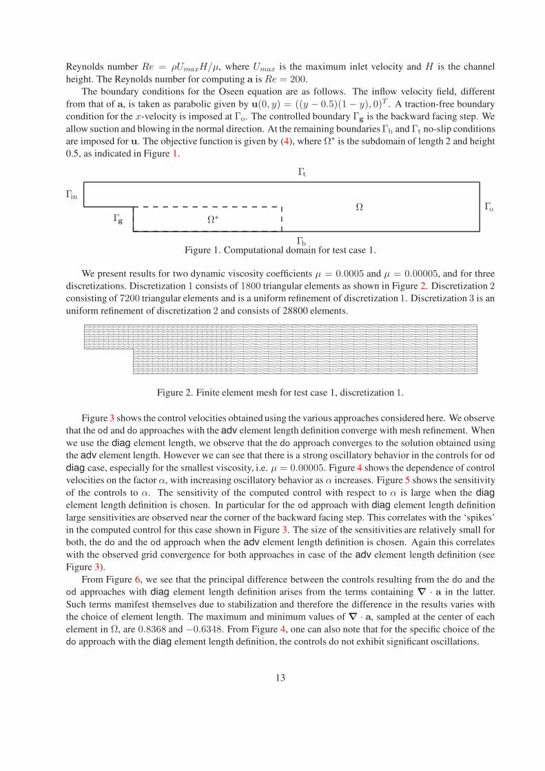
The boundary conditions for the Oseen equation are as follows. The inflow velocity field, differentfrom that of a, is taken as parabolic given by u(0, y) = ((y − 0.5)(1 − y), 0)T . A traction-free boundarycondition for the x-velocity is imposed at Γo. The controlled boundary Γg is the backward facing step. Weallow suction and blowing in the normal direction. At the remaining boundaries Γb and Γt no-slip conditionsare imposed for u. The objective function is given by (4), where Ω∗ is the subdomain of length 2 and height0.5, as indicated in Figure 1.

Γin

Γg

Γb

Γo

Γt

ΩΩ∗

Figure 1. Computational domain for test case 1.

We present results for two dynamic viscosity coefficients µ = 0.0005 and µ = 0.00005, and for threediscretizations. Discretization 1 consists of 1800 triangular elements as shown in Figure 2. Discretization 2consisting of 7200 triangular elements and is a uniform refinement of discretization 1. Discretization 3 is anuniform refinement of discretization 2 and consists of 28800 elements.

Figure 2. Finite element mesh for test case 1, discretization 1.

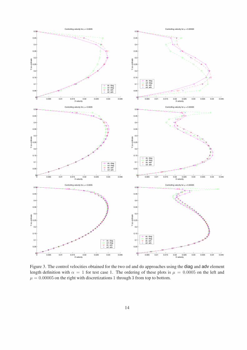
Figure 3 shows the control velocities obtained using the various approaches considered here. We observethat the od and do approaches with the adv element length definition converge with mesh refinement. Whenwe use the diag element length, we observe that the do approach converges to the solution obtained usingthe adv element length. However we can see that there is a strong oscillatory behavior in the controls for oddiag case, especially for the smallest viscosity, i.e. µ = 0.00005. Figure 4 shows the dependence of controlvelocities on the factor α, with increasing oscillatory behavior as α increases. Figure 5 shows the sensitivityof the controls to α. The sensitivity of the computed control with respect to α is large when the diagelement length definition is chosen. In particular for the od approach with diag element length definitionlarge sensitivities are observed near the corner of the backward facing step. This correlates with the ‘spikes’in the computed control for this case shown in Figure 3. The size of the sensitivities are relatively small forboth, the do and the od approach when the adv element length definition is chosen. Again this correlateswith the observed grid convergence for both approaches in case of the adv element length definition (seeFigure 3).

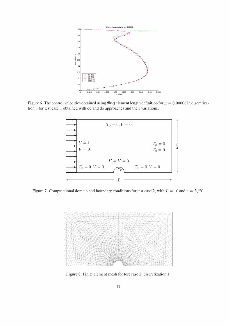
From Figure 6, we see that the principal difference between the controls resulting from the do and theod approaches with diag element length definition arises from the terms containing ∇ · a in the latter.Such terms manifest themselves due to stabilization and therefore the difference in the results varies withthe choice of element length. The maximum and minimum values of ∇ · a, sampled at the center of eachelement in Ω, are 0.8368 and −0.6348. From Figure 4, one can also note that for the specific choice of thedo approach with the diag element length definition, the controls do not exhibit significant oscillations.

13

0 0.005 0.01 0.015 0.02 0.025 0.03 0.0350

0.05

0.1

0.15

0.2

0.25

0.3

0.35

0.4

0.45

0.5

X velocity

Y c

o−or

dina

teControlling velocity for µ = 0.0005

do diagod diagdo adv od adv

0 0.005 0.01 0.015 0.02 0.025 0.03 0.035 0.04 0.0450

0.05

0.1

0.15

0.2

0.25

0.3

0.35

0.4

0.45

0.5

X velocity

Y c

o−or

dina

te

Controlling velocity for µ = 0.00005

do diagod diagdo adv od adv

0 0.005 0.01 0.015 0.02 0.025 0.03 0.0350

0.05

0.1

0.15

0.2

0.25

0.3

0.35

0.4

0.45

0.5

X velocity

Y c

o−or

dina

te

Controlling velocity for µ = 0.0005

do diagod diagdo adv od adv

0 0.005 0.01 0.015 0.02 0.025 0.03 0.035 0.04 0.0450

0.05

0.1

0.15

0.2

0.25

0.3

0.35

0.4

0.45

0.5

X velocity

Y c

o−or

dina

te

Controlling velocity for µ = 0.00005

do diagod diagdo adv od adv

0 0.005 0.01 0.015 0.02 0.025 0.03 0.0350

0.05

0.1

0.15

0.2

0.25

0.3

0.35

0.4

0.45

0.5

X velocity

Y c

o−or

dina

te

Controlling velocity for µ = 0.0005

do diagod diagdo adv od adv

0 0.005 0.01 0.015 0.02 0.025 0.03 0.035 0.04 0.0450

0.05

0.1

0.15

0.2

0.25

0.3

0.35

0.4

0.45

0.5

X velocity

Y c

o−or

dina

te

Controlling velocity for µ = 0.00005

do diagod diagdo adv od adv

Figure 3. The control velocities obtained for the two od and do approaches using the diag and adv elementlength definition with α = 1 for test case 1. The ordering of these plots is µ = 0.0005 on the left andµ = 0.00005 on the right with discretizations 1 through 3 from top to bottom.

14

−0.1 −0.08 −0.06 −0.04 −0.02 0 0.02 0.04 0.06 0.08 0.10

0.05

0.1

0.15

0.2

0.25

0.3

0.35

0.4

0.45

0.5

X velocity

Y c

o−or

dina

teControlling velocity for µ = 0.00005

od diag (α = 0.5)od diag (α = 1.0)od diag (α = 2.0)od adv (α = 1.0)

0 0.005 0.01 0.015 0.02 0.025 0.03 0.035 0.040

0.05

0.1

0.15

0.2

0.25

0.3

0.35

0.4

0.45

0.5

X velocity

Y c

o−or

dina

te

Controlling velocity for µ = 0.00005

do diag (α = 0.5)do diag (α = 1.0)do diag (α = 2.0)do adv (α = 1.0)

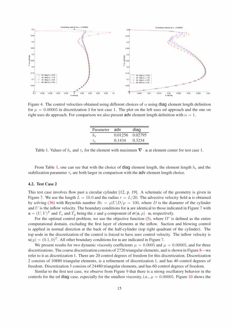
Figure 4. The control velocities obtained using different choices of α using diag element length definitionfor µ = 0.00005 in discretization 3 for test case 1. The plot on the left uses od approach and the one onright uses do approach. For comparison we also present adv element length definition with α = 1.

Parameter adv diaghe 0.01256 0.02795τe 0.1434 0.3234

Table 1. Values of he and τe for the element with maximum ∇ · a at element center for test case 1.

From Table 1, one can see that with the choice of diag element length, the element length he and thestabilization parameter τe are both larger in comparison with the adv element length choice.

4.2. Test Case 2

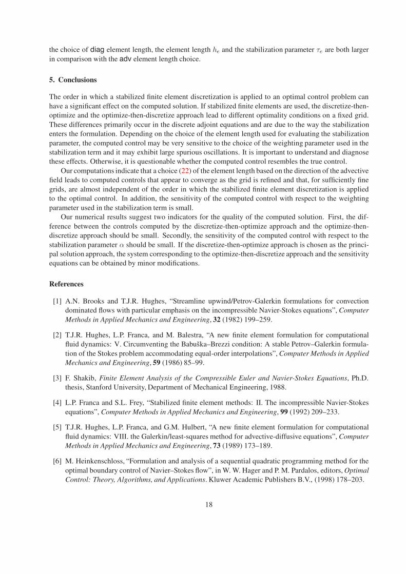
This test case involves flow past a circular cylinder [12, p. 19]. A schematic of the geometry is given inFigure 7. We use the length L = 10.0 and the radius r = L/20. The advective velocity field a is obtainedby solving (36) with Reynolds number Re = ρ|U |D/µ = 100, where D is the diameter of the cylinderand U is the inflow velocity. The boundary conditions for a are identical to those indicated in Figure 7 witha = (U, V )T and Tx and Ty being the x and y component of σ(a, p) · n, respectively.

For the optimal control problem, we use the objective function (5), where Ω∗ is defined as the entirecomputational domain, excluding the first layer of elements at the inflow. Suction and blowing controlis applied in normal direction at the back of the half-cylinder (top right quadrant of the cylinder). Thetop node in the discretization of the control is forced to have zero control velocity. The inflow velocity isu(y) = (0.1, 0)T . All other boundary conditions for u are indicated in Figure 7.

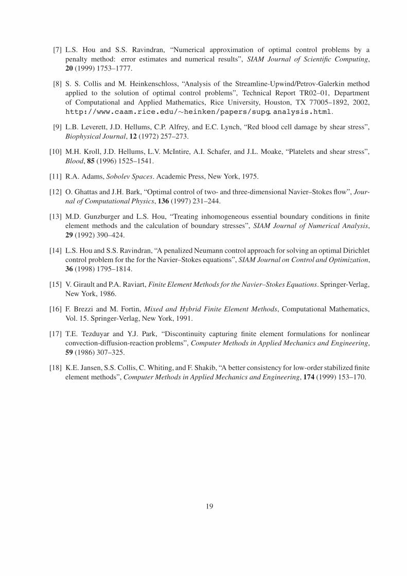
We present results for two dynamic viscosity coefficients µ = 0.0005 and µ = 0.00005, and for threediscretizations. The coarse discretization consists of 2720 triangular elements, and is shown in Figure 8—werefer to it as discretization 1. There are 20 control degrees of freedom for this discretization. Discretization2 consists of 10880 triangular elements, is a refinement of discretization 1, and has 40 control degrees offreedom. Discretization 3 consists of 24480 triangular elements, and has 60 control degrees of freedom.

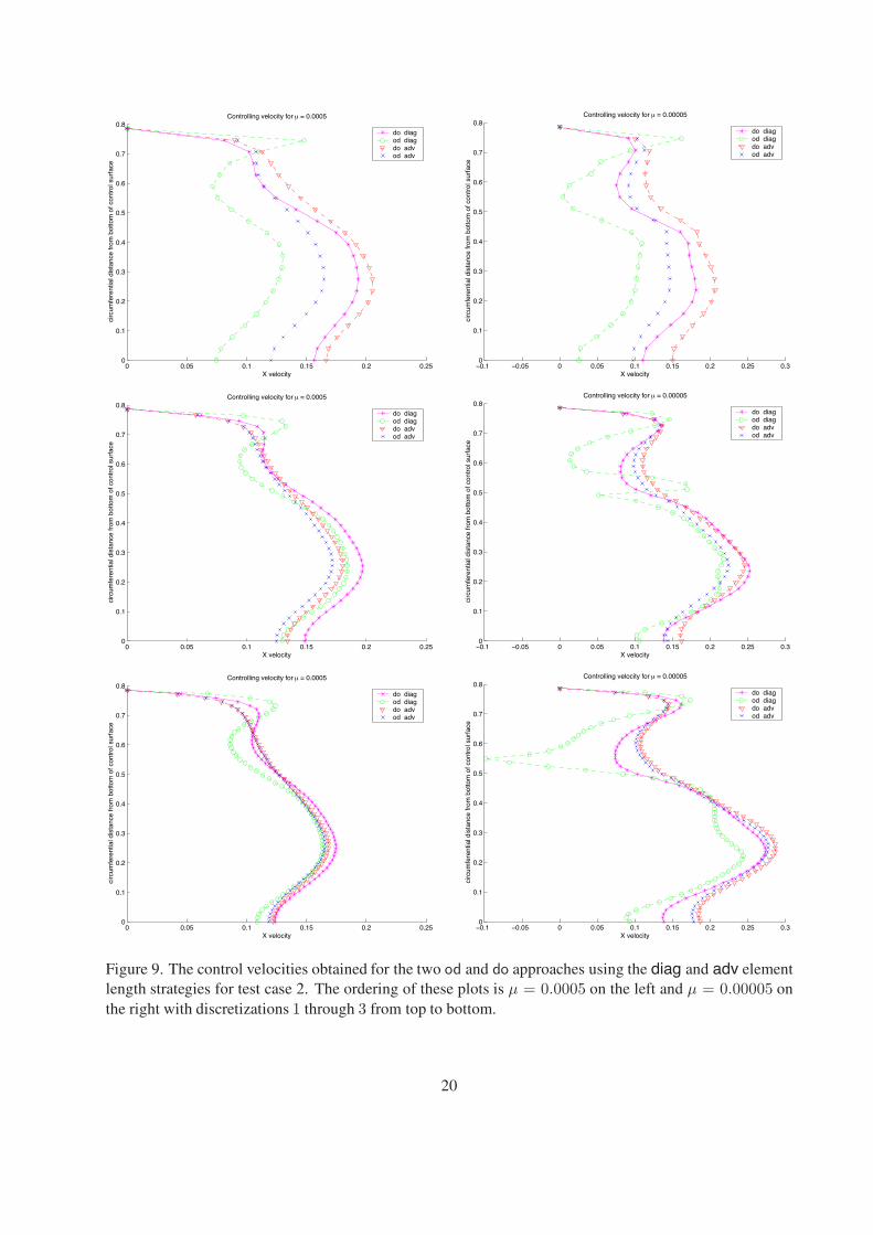
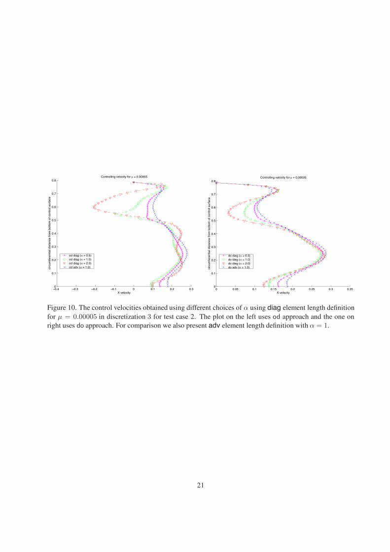
Similar to the first test case, we observe from Figure 9 that there is a strong oscillatory behavior in thecontrols for the od diag case, especially for the smallest viscosity, i.e., µ = 0.00005. Figure 10 shows the

15

0 0.1 0.2 0.3 0.4 0.5 0.6 0.70

0.05

0.1

0.15

0.2

0.25

0.3

0.35

0.4

0.45

0.5

Weighted sensitivity

Y c

o−or

dina

te Sensitivity plot for µ = 0.00005, α = 0.5

do diag od diag do adv od adv

0 0.2 0.4 0.6 0.8 1 1.2 1.40

0.05

0.1

0.15

0.2

0.25

0.3

0.35

0.4

0.45

0.5

Weighted sensitivity

Y c

o−or

dina

te

Sensitivity plot for µ = 0.00005, α = 1.0

do diag od diag do adv od adv

0 1 2 3 4 5 60

0.05

0.1

0.15

0.2

0.25

0.3

0.35

0.4

0.45

0.5

Weighted sensitivity

Y c

o−or

dina

te

Sensitivity plot for µ = 0.00005, α = 2.0

do diag od diag do adv od adv

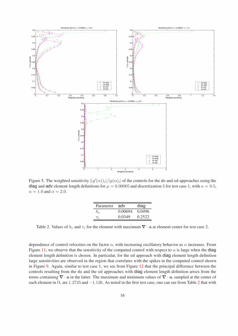
Figure 5. The weighted sensitivity |(g′(α))i|/|g(α)i| of the controls for the do and od approaches using thediag and adv element length definitions for µ = 0.00005 and discretization 3 for test case 1, with α = 0.5,α = 1.0 and α = 2.0.

Parameter adv diaghe 0.00694 0.0496τe 0.0349 0.2522

Table 2. Values of he and τe for the element with maximum ∇ · a at element center for test case 2.

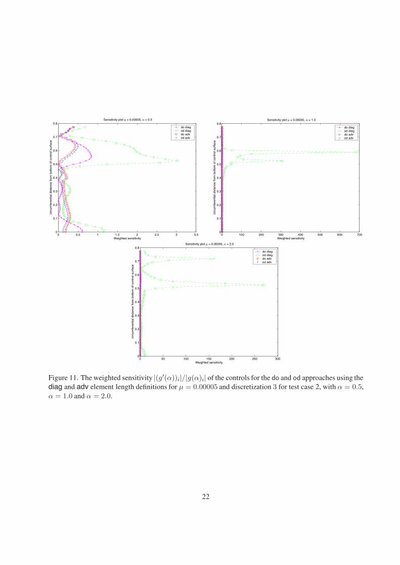
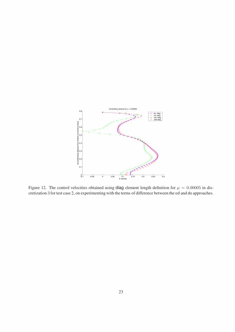
dependence of control velocities on the factor α, with increasing oscillatory behavior as α increases. FromFigure 11, we observe that the sensitivity of the computed control with respect to α is large when the diagelement length definition is chosen. In particular, for the od approach with diag element length definitionlarge sensitivities are observed in the region that correlates with the spikes in the computed control shownin Figure 9. Again, similar to test case 1, we see from Figure 12 that the principal difference between thecontrols resulting from the do and the od approaches with diag element length definition arises from theterms containing ∇ · a in the latter. The maximum and minimum values of ∇ · a, sampled at the center ofeach element in Ω, are 1.2745 and −1.126. As noted in the first test case, one can see from Table 2 that with

16

0 0.005 0.01 0.015 0.02 0.025 0.03 0.035 0.04 0.0450

0.05

0.1

0.15

0.2

0.25

0.3

0.35

0.4

0.45

0.5

X velocity

Y c

o−or

dina

te

Controlling velocity for µ = 0.00005

do diagod diagod1 diagod2 diag

Figure 6. The control velocities obtained using diag element length definition for µ = 0.00005 in discretiza-tion 3 for test case 1 obtained with od and do approaches and their variations.

L

L2

U = 1V = 0

Tx = 0, V = 0 Tx = 0, V = 0U = V = 0

Tx = 0, V = 0

Tx = 0Ty = 0

r

Figure 7. Computational domain and boundary conditions for test case 2, with L = 10 and r = L/20.

Figure 8. Finite element mesh for test case 2, discretization 1.

17

the choice of diag element length, the element length he and the stabilization parameter τe are both largerin comparison with the adv element length choice.

5. Conclusions

The order in which a stabilized finite element discretization is applied to an optimal control problem canhave a significant effect on the computed solution. If stabilized finite elements are used, the discretize-then-optimize and the optimize-then-discretize approach lead to different optimality conditions on a fixed grid.These differences primarily occur in the discrete adjoint equations and are due to the way the stabilizationenters the formulation. Depending on the choice of the element length used for evaluating the stabilizationparameter, the computed control may be very sensitive to the choice of the weighting parameter used in thestabilization term and it may exhibit large spurious oscillations. It is important to understand and diagnosethese effects. Otherwise, it is questionable whether the computed control resembles the true control.

Our computations indicate that a choice (22) of the element length based on the direction of the advectivefield leads to computed controls that appear to converge as the grid is refined and that, for sufficiently finegrids, are almost independent of the order in which the stabilized finite element discretization is appliedto the optimal control. In addition, the sensitivity of the computed control with respect to the weightingparameter used in the stabilization term is small.

Our numerical results suggest two indicators for the quality of the computed solution. First, the dif-ference between the controls computed by the discretize-then-optimize approach and the optimize-then-discretize approach should be small. Secondly, the sensitivity of the computed control with respect to thestabilization parameter α should be small. If the discretize-then-optimize approach is chosen as the princi-pal solution approach, the system corresponding to the optimize-then-discretize approach and the sensitivityequations can be obtained by minor modifications.

References

[1] A.N. Brooks and T.J.R. Hughes, “Streamline upwind/Petrov-Galerkin formulations for convectiondominated flows with particular emphasis on the incompressible Navier-Stokes equations”, ComputerMethods in Applied Mechanics and Engineering, 32 (1982) 199–259.

[2] T.J.R. Hughes, L.P. Franca, and M. Balestra, “A new finite element formulation for computationalfluid dynamics: V. Circumventing the Babuska–Brezzi condition: A stable Petrov–Galerkin formula-tion of the Stokes problem accommodating equal-order interpolations”, Computer Methods in AppliedMechanics and Engineering, 59 (1986) 85–99.

[3] F. Shakib, Finite Element Analysis of the Compressible Euler and Navier-Stokes Equations, Ph.D.thesis, Stanford University, Department of Mechanical Engineering, 1988.

[4] L.P. Franca and S.L. Frey, “Stabilized finite element methods: II. The incompressible Navier-Stokesequations”, Computer Methods in Applied Mechanics and Engineering, 99 (1992) 209–233.

[5] T.J.R. Hughes, L.P. Franca, and G.M. Hulbert, “A new finite element formulation for computationalfluid dynamics: VIII. the Galerkin/least-squares method for advective-diffusive equations”, ComputerMethods in Applied Mechanics and Engineering, 73 (1989) 173–189.

[6] M. Heinkenschloss, “Formulation and analysis of a sequential quadratic programming method for theoptimal boundary control of Navier–Stokes flow”, in W. W. Hager and P. M. Pardalos, editors, OptimalControl: Theory, Algorithms, and Applications. Kluwer Academic Publishers B.V., (1998) 178–203.

18

[7] L.S. Hou and S.S. Ravindran, “Numerical approximation of optimal control problems by apenalty method: error estimates and numerical results”, SIAM Journal of Scientific Computing,20 (1999) 1753–1777.

[8] S. S. Collis and M. Heinkenschloss, “Analysis of the Streamline-Upwind/Petrov-Galerkin methodapplied to the solution of optimal control problems”, Technical Report TR02–01, Departmentof Computational and Applied Mathematics, Rice University, Houston, TX 77005–1892, 2002,http://www.caam.rice.edu/∼heinken/papers/supg analysis.html.

[9] L.B. Leverett, J.D. Hellums, C.P. Alfrey, and E.C. Lynch, “Red blood cell damage by shear stress”,Biophysical Journal, 12 (1972) 257–273.

[10] M.H. Kroll, J.D. Hellums, L.V. McIntire, A.I. Schafer, and J.L. Moake, “Platelets and shear stress”,Blood, 85 (1996) 1525–1541.

[11] R.A. Adams, Sobolev Spaces. Academic Press, New York, 1975.

[12] O. Ghattas and J.H. Bark, “Optimal control of two- and three-dimensional Navier–Stokes flow”, Jour-nal of Computational Physics, 136 (1997) 231–244.

[13] M.D. Gunzburger and L.S. Hou, “Treating inhomogeneous essential boundary conditions in finiteelement methods and the calculation of boundary stresses”, SIAM Journal of Numerical Analysis,29 (1992) 390–424.

[14] L.S. Hou and S.S. Ravindran, “A penalized Neumann control approach for solving an optimal Dirichletcontrol problem for the for the Navier–Stokes equations”, SIAM Journal on Control and Optimization,36 (1998) 1795–1814.

[15] V. Girault and P.A. Raviart, Finite Element Methods for the Navier–Stokes Equations. Springer-Verlag,New York, 1986.

[16] F. Brezzi and M. Fortin, Mixed and Hybrid Finite Element Methods, Computational Mathematics,Vol. 15. Springer-Verlag, New York, 1991.

[17] T.E. Tezduyar and Y.J. Park, “Discontinuity capturing finite element formulations for nonlinearconvection-diffusion-reaction problems”, Computer Methods in Applied Mechanics and Engineering,59 (1986) 307–325.

[18] K.E. Jansen, S.S. Collis, C. Whiting, and F. Shakib, “A better consistency for low-order stabilized finiteelement methods”, Computer Methods in Applied Mechanics and Engineering, 174 (1999) 153–170.

19

0 0.05 0.1 0.15 0.2 0.250

0.1

0.2

0.3

0.4

0.5

0.6

0.7

0.8

X velocity

circ

umfe

rent

ial d

ista

nce

from

bot

tom

of c

ontr

ol s

urfa

ceControlling velocity for µ = 0.0005

do diagod diagdo adv od adv

−0.1 −0.05 0 0.05 0.1 0.15 0.2 0.25 0.30

0.1

0.2

0.3

0.4

0.5

0.6

0.7

0.8

X velocity

circ

umfe

rent

ial d

ista

nce

from

bot

tom

of c

ontr

ol s

urfa

ce

Controlling velocity for µ = 0.00005

do diagod diagdo adv od adv

0 0.05 0.1 0.15 0.2 0.250

0.1

0.2

0.3

0.4

0.5

0.6

0.7

0.8

X velocity

circ

umfe

rent

ial d

ista

nce

from

bot

tom

of c

ontr

ol s

urfa

ce

Controlling velocity for µ = 0.0005

do diagod diagdo adv od adv

−0.1 −0.05 0 0.05 0.1 0.15 0.2 0.25 0.30

0.1

0.2

0.3

0.4

0.5

0.6

0.7

0.8

X velocity

circ

umfe

rent

ial d

ista

nce

from

bot

tom

of c

ontr

ol s

urfa

ce

Controlling velocity for µ = 0.00005

do diagod diagdo adv od adv

0 0.05 0.1 0.15 0.2 0.250

0.1

0.2

0.3

0.4

0.5

0.6

0.7

0.8

X velocity

circ

umfe

rent

ial d

ista

nce

from

bot

tom

of c

ontr

ol s

urfa

ce

Controlling velocity for µ = 0.0005

do diagod diagdo adv od adv

−0.1 −0.05 0 0.05 0.1 0.15 0.2 0.25 0.30

0.1

0.2

0.3

0.4

0.5

0.6

0.7

0.8

X velocity

circ

umfe

rent

ial d

ista

nce

from

bot

tom

of c

ontr

ol s

urfa

ce

Controlling velocity for µ = 0.00005

do diagod diagdo adv od adv

Figure 9. The control velocities obtained for the two od and do approaches using the diag and adv elementlength strategies for test case 2. The ordering of these plots is µ = 0.0005 on the left and µ = 0.00005 onthe right with discretizations 1 through 3 from top to bottom.

20

−0.4 −0.3 −0.2 −0.1 0 0.1 0.2 0.30

0.1

0.2

0.3

0.4

0.5

0.6

0.7

0.8

X velocity

circ

umfe

rent

ial d

ista

nce

from

bot

tom

of c

ontr

ol s

urfa

ce

Controlling velocity for µ = 0.00005

od diag (α = 0.5)od diag (α = 1.0)od diag (α = 2.0)od adv (α = 1.0)

0 0.05 0.1 0.15 0.2 0.25 0.3 0.350

0.1

0.2

0.3

0.4

0.5

0.6

0.7

0.8

X velocity

circ

umfe

rent

ial d

ista

nce

from

bot

tom

of c

ontr

ol s

urfa

ce

Controlling velocity for µ = 0.00005

do diag (α = 0.5)do diag (α = 1.0)do diag (α = 2.0)do adv (α = 1.0)

Figure 10. The control velocities obtained using different choices of α using diag element length definitionfor µ = 0.00005 in discretization 3 for test case 2. The plot on the left uses od approach and the one onright uses do approach. For comparison we also present adv element length definition with α = 1.

21

0 0.5 1 1.5 2 2.5 3 3.50

0.1

0.2

0.3

0.4

0.5

0.6

0.7

0.8

Weighted sensitivity

circ

umfe

rent

ial d

ista

nce

from

bot

tom

of c

ontr

ol s

urfa

ce

Sensitivity plot µ = 0.00005, α = 0.5

do diag od diag do adv od adv

0 100 200 300 400 500 600 7000

0.1

0.2

0.3

0.4

0.5

0.6

0.7

0.8

Weighted sensitivity

circ

umfe

rent

ial d

ista

nce

from

bot

tom

of c

ontr

ol s

urfa

ce

Sensitivity plot µ = 0.00005, α = 1.0

do diag od diag do adv od adv

0 50 100 150 200 250 3000

0.1

0.2

0.3

0.4

0.5

0.6

0.7

0.8

Weighted sensitivity

circ

umfe

rent

ial d

ista

nce

from

bot

tom

of c

ontr

ol s

urfa

ce

Sensitivity plot µ = 0.00005, α = 2.0

do diag od diag do adv od adv

Figure 11. The weighted sensitivity |(g′(α))i|/|g(α)i| of the controls for the do and od approaches using thediag and adv element length definitions for µ = 0.00005 and discretization 3 for test case 2, with α = 0.5,α = 1.0 and α = 2.0.

22

−0.1 −0.05 0 0.05 0.1 0.15 0.2 0.25 0.30

0.1

0.2

0.3

0.4

0.5

0.6

0.7

0.8

X velocity

circ

umfe

rent

ial d

ista

nce

from

bot

tom

of c

ontr

ol s

urfa

ce

Controlling velocity for µ = 0.00005

do diagod diagod1 diagod2 diag

Figure 12. The control velocities obtained using diag element length definition for µ = 0.00005 in dis-cretization 3 for test case 2, on experimenting with the terms of difference between the od and do approaches.

23