arXiv:math/0407298v1 [math.AC] 16 Jul 2004 TETRAHEDRAL CURVES J. MIGLIORE * , U. NAGEL + Abstract. A tetrahedral curve is a space curve whose defining ideal is an intersection of powers of monomial prime ideals of height two. It is supported on a tetrahedral configuration of lines. Schwartau described when certain such curves are ACM, namely he restricted to curves supported on a certain four of the six lines. We consider the general situation. We first show that starting with an arbitrary tetrahedral curve, there is a particular reduction that produces a smaller tetrahedral curve and preserves the even liaison class. We call the curves that are minimal with respect to this reduction S-minimal curves. Given a tetrahedral curve, we describe a simple algorithm (involving only integers) that computes the S-minimal curve of the corresponding even liaison class; in the process it determines if the original curve is arithmetically Cohen-Macaulay or not. We also describe the minimal free resolution of an S-minimal curve, using the theory of cellular resolutions. This resolution is always linear. This result allows us to classify the arith- metically Buchsbaum, non-ACM tetrahedral curves. More importantly, it allows us to conclude that an S-minimal curve is minimal in its even liaison class; that is, the whole even liaison class can be built up from the S-minimal curve. Finally, we show that there is a large set of S-minimal curves such that each curve corresponds to a smooth point of a component of the Hilbert scheme and that this component has the expected dimension. Contents 1. Introduction 2 2. Background 3 3. Reduction and S-minimality 5 4. The Minimal Free Resolution of an S-minimal Curve 9 5. Minimality in the Even Liaison Class, and Applications 14 6. Unobstructedness of some curves 19 7. Remarks and problems 25 Appendix: The algorithm to find S -minimal curves 27 References 30 * Part of the work for this paper was done while this author was sponsored by the National Security Agency under Grant Number MDA904-03-1-0071. + This author gratefully acknowledges partial support by a Special Faculty Research Fellowship from the University of Kentucky. 1

Welcome message from author
This document is posted to help you gain knowledge. Please leave a comment to let me know what you think about it! Share it to your friends and learn new things together.
Transcript

arX
iv:m
ath/
0407
298v
1 [
mat
h.A
C]
16
Jul 2
004
TETRAHEDRAL CURVES
J. MIGLIORE∗, U. NAGEL+
Abstract. A tetrahedral curve is a space curve whose defining ideal is an intersectionof powers of monomial prime ideals of height two. It is supported on a tetrahedralconfiguration of lines. Schwartau described when certain such curves are ACM, namelyhe restricted to curves supported on a certain four of the six lines. We consider thegeneral situation.
We first show that starting with an arbitrary tetrahedral curve, there is a particularreduction that produces a smaller tetrahedral curve and preserves the even liaison class.We call the curves that are minimal with respect to this reduction S-minimal curves.Given a tetrahedral curve, we describe a simple algorithm (involving only integers) thatcomputes the S-minimal curve of the corresponding even liaison class; in the processit determines if the original curve is arithmetically Cohen-Macaulay or not. We alsodescribe the minimal free resolution of an S-minimal curve, using the theory of cellularresolutions. This resolution is always linear. This result allows us to classify the arith-metically Buchsbaum, non-ACM tetrahedral curves. More importantly, it allows us toconclude that an S-minimal curve is minimal in its even liaison class; that is, the wholeeven liaison class can be built up from the S-minimal curve. Finally, we show that thereis a large set of S-minimal curves such that each curve corresponds to a smooth point ofa component of the Hilbert scheme and that this component has the expected dimension.
Contents
1. Introduction 22. Background 33. Reduction and S-minimality 54. The Minimal Free Resolution of an S-minimal Curve 95. Minimality in the Even Liaison Class, and Applications 146. Unobstructedness of some curves 197. Remarks and problems 25Appendix: The algorithm to find S-minimal curves 27References 30
∗ Part of the work for this paper was done while this author was sponsored by the National SecurityAgency under Grant Number MDA904-03-1-0071.+ This author gratefully acknowledges partial support by a Special Faculty Research Fellowship from theUniversity of Kentucky.
1

2 J. MIGLIORE, U. NAGEL
1. Introduction
In his Ph.D. thesis [20], which was never published, Phil Schwartau considered certainmonomial ideals and the question of whether or not they were Cohen-Macaulay. Specifi-cally, he considered ideals of the form
(X0, X1)a ∩ (X1, X2)
b ∩ (X2, X3)c ∩ (X3, X0)
d
in the ring k[X0, X1, X2, X3] where k is an algebraically closed field. These are unmixedideals defining curves in P
3. They are supported on a complete intersection (taking(a, b, c, d) = (1, 1, 1, 1) gives the complete intersection of X0X2 and X1X3). Schwartaugave a complete classification of the 4-tuples of integers (a, b, c, d) that define arithmeti-cally Cohen-Macaulay curves (see Theorem 2.4 and Theorem 5.3).
This paper arose from our desire to make the natural extension of this result to includethe lines defined by (X0, X2) and (X1, X3). To simplify the notation we have changed thevariables, so we are considering the ring R = k[a, b, c, d] and ideals of the form
I = (a, b)a1 ∩ (a, c)a2 ∩ (a, d)a3 ∩ (b, c)a4 ∩ (b, d)a5 ∩ (c, d)a6.
Note that I is an unmixed monomial ideal. Since these six lines can be viewed as formingthe edges of a tetrahedron, we call such a curve a tetrahedral curve. It is useful to considerthe empty set as the trivial curve defined by (0, 0, 0, 0, 0, 0).
More than simply considering the question of when such a curve is arithmetically Cohen-Macaulay, we are interested in getting some idea of the even liaison class of such a curve.For background on liaison, see the book [12]; for the most part we will assume the necessarydefinitions and basic results on liaison.
Many papers in the literature give classification results of the following kind: theyconsider a particular kind of curve, and ask when two such curves are linked, or askfor a description of the even liaison class of such a curve (cf. for instance [5], [13], [14],[18]). The work in this paper can be viewed, in part, as a new contribution to this kindof question. However, the main interest comes from the naturalness of these monomialideals themselves, from the surprising effectiveness of our reduction procedure, from thesimplicity of the minimal free resolution obtained, and from the interplay of strikinglydifferent techniques and tools used to obtain these results.
The key idea that got this work started was a realization that there is a simple reductionpossible for tetrahedral curves (Proposition 3.1). Using the machinery of basic doublelinks, this reduction accomplishes two amazing things: the new curve is in the same evenliaison class as the original curve, and the new curve is again a tetrahedral curve, butsmaller!
Using this reduction, one of two things happens: either the process of reduction contin-ues until the curve vanishes, i.e. we get the trivial curve, or the process stops at a curvethat cannot be further reduced in this way. The curves that ultimately reduce to the triv-ial curve are clearly arithmetically Cohen-Macaulay, thanks to liaison theory. Curves thatcannot be further reduced in this way are very important, and we call them S-minimal
curves. We give a numerical criterion for S-minimality (Corollary 3.5 and Lemma 3.8).This leads to a simple algorithm (easily done by hand) for computing an S-minimal curvestarting with any tetrahedral curve. A MAPLE implementation of it is documented inthe appendix.

TETRAHEDRAL CURVES 3
The first main result of this paper is Theorem 4.2, where the minimal free resolution ofan S-minimal tetrahedral curve is computed. We show, in particular, that this resolutionis linear. This proof starts by finding the minimal generators of the ideal, and then ittranslates these generators into a cell complex and uses the theory of cellular resolutionsas developed in [2] to find the rest of the resolution.
An immediate consequence of this result is that an S-minimal curve is arithmeticallyCohen-Macaulay if and only if it is trivial. This allows one to easily determine, forany 6-tuple of integers (a1, a2, a3, a4, a5, a6), whether it corresponds to an arithmeticallyCohen-Macaulay curve or not. Another easy consequence is that a tetrahedral curveis arithmetically Buchsbaum if and only if its Hartshorne-Rao module has diameter 1.(It was already known by Schwartau that certain arithmetically Buchsbaum tetrahedralcurves existed.)
A much deeper consequence of Theorem 4.2 is the second main result of the paper(Theorem 5.1), which says that a tetrahedral curve C is S-minimal if and only if it isminimal in its even liaison class.
We give two applications of this result. The first, Theorem 5.3, is a new proof ofSchwartau’s theorem classifying the arithmetically Cohen-Macaulay curves supported onthe complete intersection by giving the precise set of 4-tuples. The second application,Corollary 5.4, is a classification of the 6-tuples that define minimal tetrahedral curvesthat are arithmetically Buchsbaum. Both of these applications primarily use the earlierresults described above, but need the minimality in the even liaison class to complete theproof.
Our third main line of investigation concerns the question of unobstructedness and thesearch for nice components of the Hilbert scheme. (A component is said to be “nice” ifit has the expected dimension 4 · degC.) A great deal of work has been done concerningnice components of the Hilbert scheme – we refer the reader to [7] and to [9], bothfor important results along these lines, and also for numerous references to other work.Using the method of Dolcetti in [7], we first prove that any curve in P
3 with linearresolution and Hartshorne-Rao module of diameter ≤ 2 is unobstructed, and its Hilbertscheme has the expected dimension 4 · degC (Proposition 6.1). We then characterize the6-tuples corresponding to minimal tetrahedral curves with Hartshorne-Rao modules ofdiameter ≤ 2 (Corollary 5.4 and Lemma 6.2), which then are unobstructed. Turning toa different kind of minimal tetrahedral curve, we show that a tetrahedral curve definedby (a1, 0, 0, 0, 0, a6) is also unobstructed. Since we have shown the unobstructedness of alarge class of minimal tetrahedral curves, and have shown experimentally on the computerthat others are also unobstructed, we end with the question of whether in fact all minimaltetrahedral curves are unobstructed.
We end the paper with a number of questions that arise naturally from our work.
2. Background
Let R = k[a, b, c, d], where k is a field. We abbreviate by ACM the term “arithmeti-cally Cohen-Macaulay.” Recall that a projective subscheme V is ACM if and only if thedeficiency modules all vanish:
H i(Pn, IV (t)) = 0 for all t ∈ Z and all 1 ≤ i ≤ dimV .
4 J. MIGLIORE, U. NAGEL
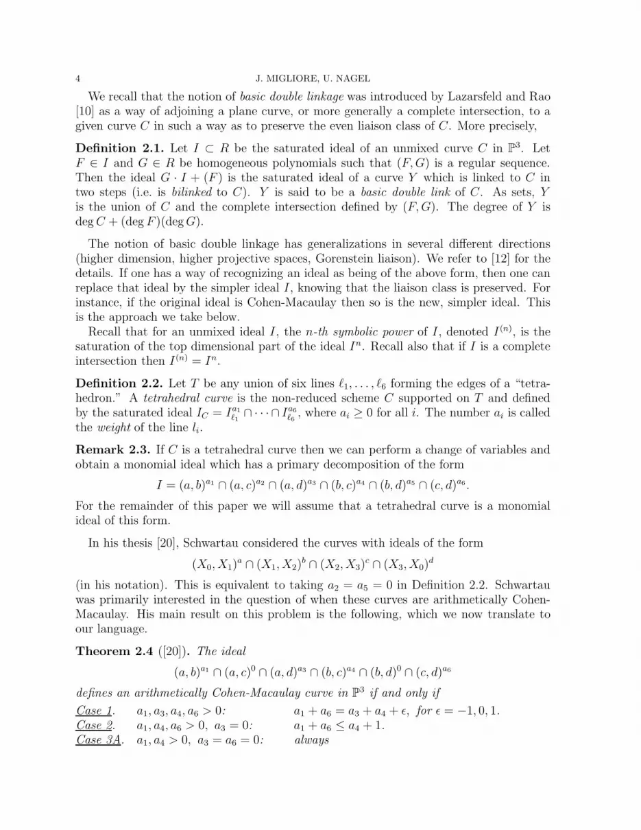
We recall that the notion of basic double linkage was introduced by Lazarsfeld and Rao[10] as a way of adjoining a plane curve, or more generally a complete intersection, to agiven curve C in such a way as to preserve the even liaison class of C. More precisely,
Definition 2.1. Let I ⊂ R be the saturated ideal of an unmixed curve C in P3. Let
F ∈ I and G ∈ R be homogeneous polynomials such that (F,G) is a regular sequence.Then the ideal G · I + (F ) is the saturated ideal of a curve Y which is linked to C intwo steps (i.e. is bilinked to C). Y is said to be a basic double link of C. As sets, Yis the union of C and the complete intersection defined by (F,G). The degree of Y isdegC + (deg F )(degG).
The notion of basic double linkage has generalizations in several different directions(higher dimension, higher projective spaces, Gorenstein liaison). We refer to [12] for thedetails. If one has a way of recognizing an ideal as being of the above form, then one canreplace that ideal by the simpler ideal I, knowing that the liaison class is preserved. Forinstance, if the original ideal is Cohen-Macaulay then so is the new, simpler ideal. Thisis the approach we take below.
Recall that for an unmixed ideal I, the n-th symbolic power of I, denoted I(n), is thesaturation of the top dimensional part of the ideal In. Recall also that if I is a completeintersection then I(n) = In.
Definition 2.2. Let T be any union of six lines ℓ1, . . . , ℓ6 forming the edges of a “tetra-hedron.” A tetrahedral curve is the non-reduced scheme C supported on T and definedby the saturated ideal IC = Ia1ℓ1 ∩ · · · ∩ Ia6ℓ6 , where ai ≥ 0 for all i. The number ai is calledthe weight of the line li.
Remark 2.3. If C is a tetrahedral curve then we can perform a change of variables andobtain a monomial ideal which has a primary decomposition of the form
I = (a, b)a1 ∩ (a, c)a2 ∩ (a, d)a3 ∩ (b, c)a4 ∩ (b, d)a5 ∩ (c, d)a6.
For the remainder of this paper we will assume that a tetrahedral curve is a monomialideal of this form.
In his thesis [20], Schwartau considered the curves with ideals of the form
(X0, X1)a ∩ (X1, X2)
b ∩ (X2, X3)c ∩ (X3, X0)
d
(in his notation). This is equivalent to taking a2 = a5 = 0 in Definition 2.2. Schwartauwas primarily interested in the question of when these curves are arithmetically Cohen-Macaulay. His main result on this problem is the following, which we now translate toour language.
Theorem 2.4 ([20]). The ideal
(a, b)a1 ∩ (a, c)0 ∩ (a, d)a3 ∩ (b, c)a4 ∩ (b, d)0 ∩ (c, d)a6
defines an arithmetically Cohen-Macaulay curve in P3 if and only if
Case 1. a1, a3, a4, a6 > 0: a1 + a6 = a3 + a4 + ǫ, for ǫ = −1, 0, 1.Case 2. a1, a4, a6 > 0, a3 = 0: a1 + a6 ≤ a4 + 1.Case 3A. a1, a4 > 0, a3 = a6 = 0: always

TETRAHEDRAL CURVES 5
Case 3B. a1, a6 > 0, a3 = a4 = 0: never
Case 4. a1 > 0, a3 = a4 = a6 = 0: always
Remark 2.5. Clearly Schwartau intended some kind of reduction of cases, since forinstance the case a2 > 0, a1 = a3 = a4 = 0 is not included in his theorem. We havegiven an “invariant” version in Theorem 5.3 below, which we think reflects Schwartau’sintention. We also give a new proof.
3. Reduction and S-minimality
The key to our approach to this problem is the following reduction method.
Proposition 3.1. Let I = (a, b)a1 ∩ (a, c)a2 ∩ (a, d)a3 ∩ (b, c)a4 ∩ (b, d)a5 ∩ (c, d)a6 where
not all exponents ai are zero. Consider the following systems of inequalities:
(A) : a1 + a2 ≥ a4,a1 + a3 ≥ a5,a2 + a3 ≥ a6
(B) : a1 + a4 ≥ a2,a1 + a5 ≥ a3,a4 + a5 ≥ a6
(C) : a2 + a4 ≥ a1,a2 + a6 ≥ a3,a4 + a6 ≥ a5
(D) : a3 + a5 ≥ a1,a3 + a6 ≥ a2,a5 + a6 ≥ a4.
For 1 ≤ i ≤ 6 let a′i = max{0, ai − 1}. Then we have
(i) (A) ⇔ I is a basic double link of
(a, b)a′
1 ∩ (a, c)a′
2 ∩ (a, d)a′
3 ∩ (b, c)a4 ∩ (b, d)a5 ∩ (c, d)a6
using F = ba1ca2da3 and G = a.(ii) (B) ⇔ I is a basic double link of
(a, b)a′
1 ∩ (a, c)a2 ∩ (a, d)a3 ∩ (b, c)a′
4 ∩ (b, d)a′
5 ∩ (c, d)a6.
using F = aa1ca4da5 and G = b.(iii) (C) ⇔ I is a basic double link of
(a, b)a1 ∩ (a, c)a′
2 ∩ (a, d)a3 ∩ (b, c)a′
4 ∩ (b, d)a5 ∩ (c, d)a′
6.
using F = aa2ba4da6 and G = c.(iv) (D) ⇔ I is a basic double link of
(a, b)a1 ∩ (a, c)a2 ∩ (a, d)a′
3 ∩ (b, c)a4 ∩ (b, d)a′
5 ∩ (c, d)a′
6.
using F = aa3ba5ca6 and G = d.
Proof. We will prove (i); of course the others are proved similarly. First note that
a · (a, b)n−1 + (bn) = (a, b)n
for n ≥ 1. Now consider the monomial F = ba1ca2da3 . Notice that
(3.1) F ∈ (a, b)a1 ∩ (a, c)a2 ∩ (a, d)a3 ⊂ (a, b)a′
1 ∩ (a, c)a′
2 ∩ (a, d)a′
3
even when one or more of the ai = 0. The three inequalities are equivalent to
(3.2) F ∈ (b, c)a4 ∩ (b, d)a5 ∩ (c, d)a6.

6 J. MIGLIORE, U. NAGEL
Hence
F ∈ (a, b)a′
1 ∩ (a, c)a′
2 ∩ (a, d)a′
3 ∩ (b, c)a4 ∩ (b, d)a5 ∩ (c, d)a6 .
Notice that (a, F ) is a regular sequence. Hence we can construct a basic double link ofthe form
J = a ·[
(a, b)a′
1 ∩ (a, c)a′
2 ∩ (a, d)a′
3 ∩ (b, c)a4 ∩ (b, d)a5 ∩ (c, d)a6]
+ (ba1ca2da3).
We have to show that
J = I = (a, b)a1 ∩ (a, c)a2 ∩ (a, d)a3 ∩ (b, c)a4 ∩ (b, d)a5 ∩ (c, d)a6 .
The ideal J is a saturated, unmixed ideal, by the theory of basic double linkage (cf. [12]),so it is enough to show that J ⊂ I and that they define schemes of the same degree.
For the first one, the fact that
a ·[(a, b)a
′
1 ∩ (a, c)a′
2 ∩ (a, d)a′
3 ∩ (b, c)a4 ∩ (b, d)a5 ∩ (c, d)a6]
⊆ (a, b)a1 ∩ (a, c)a2 ∩ (a, d)a3 ∩ (b, c)a4 ∩ (b, d)a5 ∩ (c, d)a6
is clear, while the fact that ba1ca2da3 ∈ I comes from (3.1) and (3.2) above.For the degree computation, recall that
(n
2
)+ n =
(n+1
2
). Then, again using the theory
of basic double linkage, the degree of J is
deg J =
(a1
2
)
+
(a2
2
)
+
(a3
2
)
+
(a4 + 1
2
)
+
(a5 + 1
2
)
+
(a6 + 1
2
)
+ (a1 + a2 + a3)
=
(a1 + 1
2
)
+
(a2 + 1
2
)
+
(a3 + 1
2
)
+
(a4 + 1
2
)
+
(a5 + 1
2
)
+
(a6 + 1
2
)
= deg I
as desired.The converse is immediate: the fact that I is a basic double link as stated implies the
inequalities of (A) by again using(3.1) and (3.2). �
Notation 3.2. For the rest of this paper we will abbreviate the monomial ideal
(a, b)a1 ∩ (a, c)a2 ∩ (a, d)a3 ∩ (b, c)a4 ∩ (b, d)a5 ∩ (c, d)a6
(or the corresponding curve) by the 6-tuple (a1, a2, a3, a4, a5, a6).
Remark 3.3. Basic double linkage is a special case of Schwartau’s “liaison addition.”(See [20] for the original and [8] for a generalization.) Without entering into details, weremark that many interesting tetrahedral curves arise as liaison additions. For instance,let I be the ideal of the six lines, i.e. the tetrahedral curve (1, 1, 1, 1, 1, 1). Let F be thepolynomial abcd giving the four faces of the “tetrahedron” defined by I. Note that F isdouble along each of the six lines. Let G be a generally chosen cubic in I. Then (F,G)self-links I (as can be see geometrically, using Bezout’s theorem) and one can check thatin fact the d-th symbolic power of I, I(d), can be expressed as
I(d) = Gd−1 · I + F · I(d−2).
Hence we see directly the curves (d, d, d, d, d, d) are ACM. Note however, that the d-thpower Id is not saturated, and has embedded points.

TETRAHEDRAL CURVES 7
Schwartau also obtains many Buchsbaum curves using liaison addition. We will returnto Buchsbaum curves below.
Definition 3.4. We say that a tetrahedral curve is S-minimal if there is no reduction ofthe type described in Proposition 3.1.
Corollary 3.5. Consider a tetrahedral curve C = (a1, a2, a3, a4, a5, a6) where not all aiare 0. Assume without loss of generality that a6 = max{a1, . . . , a6}. Then C is S-minimal
if and only ifa1 > max{a3 + a5, a2 + a4} and
a6 > max{a4 + a5, a2 + a3}
Proof. It is immediate to check that if the stated conditions are satisfied then each of (A),(B), (C) and (D) in Proposition 3.1 has at least one inequality that is not satisfied, henceC cannot be reduced via Proposition 3.1.
Conversely, suppose that C is S-minimal. The second and third inequalities of (C) and(D) in Proposition 3.1are forced to be true by the assumption that a6 = max{a1, . . . , a6},so S-minimal implies that a1 > max{a3 + a5, a2 + a4}. In particular, a1 > a2, a1 > a3,a1 > a4 and a1 > a5, so the first two inequalities of (A) and of (B) must be true. Henceagain the assumption that C is S-minimal forces a6 > max{a4 + a5, a2 + a3}. �
Example 3.6. Even with the assumption that a6 = max{a1, . . . , a6}, the first inequal-ity of Corollary 3.5 alone does not imply S-minimality, as shown by the example C =(4, 2, 2, 1, 1, 4), which can be reduced using (A) to the curve C ′ = (3, 1, 1, 1, 1, 4). Thisnew curve C ′ is S-minimal. It can be checked that C ′ (and hence C) is not arithmeticallyCohen-Macaulay (see Corollary 4.3 as well).
Our next goal is to provide an algorithm that produces an S-minimal curve to a giventetrahedral curve C. To this end we will extend the definition of weights. We will use thetetrahedron T = T (C) whose edges are part of the (potentially) supporting lines of thecurve C.
Definition 3.7. The weight of a facet of T = T (C) is the sum of the weights of the edgesforming its boundary. Similarly, the weight of a pair of skew lines being a subset of thesix given lines is the sum of the weights of the lines.
Using these concepts we can make Corollary 3.5 more precise. Note that each of thereductions (A) - (D) in Proposition 3.1 reduces the weights of the edges of a facet ofthe tetrahedron. Thus, we will say that we reduce a facet if we apply the correspondingreduction.
The next result says in particular that a tetrahedral curve is not minimal if and only ifwe can reduce a facet of maximal weight.
Lemma 3.8. Let C be a tetrahedral curve C = (a1, a2, a3, a4, a5, a6) where we assume
without loss of generality that a6 = max{a1, . . . , a6} > 0. Let w be the maximal weight of
a facet of the tetrahedron T = T (C). Then the following conditions are equivalent:
(a) C is not S-minimal.
(b) a1 + a6 ≤ w.
(c) One can reduce any of the facets of T having maximal weight w.

8 J. MIGLIORE, U. NAGEL
Proof. We begin by showing the equivalence of (a) and (b). According to Corollary 3.5we know that C is not S-minimal if and only if
a1 ≤ max{a3 + a5, a2 + a4} ora6 ≤ max{a4 + a5, a2 + a3}.
But this is equivalent to the condition
a1 + a6 ≤ max{a1 + a4 + a5, a1 + a2 + a3, a3 + a5 + a6, a2 + a4 + a6} = w
as claimed.Since (c) trivially implies (a), it remains to show that (c) is a consequence of (b). To
this end we distinguish four cases.Case 1: Let w = a3 + a5 + a6. Then (b) provides a3 + a5 ≥ a1 showing that we can
apply reduction (D).Case 2: Let w = a2 + a4 + a6. Then we conclude as above that we can use reduction
(C).Case 3: Let w = a1 + a2 + a3. Then (b) implies a2 + a3 ≥ a6. Moreover, we have by
assumption w ≥ a2 + a4 + a6. It implies
a1 + a3 ≥ a4 + a6 ≥ a6 ≥ a5.
Similarly w ≥ a3 +a5 +a6 provides a1 +a2 ≥ a4. Thus, we have shown that we can applyreduction (A).
Case 4: Let w = a1 + a4 + a5. Then we see as in Case 3 that we can use reduction(B). �
The last result leads to an algorithm for producing S-minimal curves that works withweights only.
Algorithm 3.9 (for computing S-minimal curves).Input: (a1, . . . , a6) ∈ Z
6 where all ai ≥ 0, the weight vector of a tetrahedral curve C.Output: (a1, . . . , a6), the weight vector of an S-minimal curve obtained by reducing C.
1. compute i such that ai = max{a1, . . . , a6}
2. if ai = 0 then return (0, . . . , 0)
3. determine a facet F of maximal weight w
4. if ai + a7−i > w then return (a1, . . . , a6).
5. apply the reduction corresponding to the facet F and go to Step 1
Remark 3.10. (i) Strictly speaking the scheme above is not an algorithm since it leaveschoices in Steps 1 and 3 in case there is more than one line or facet of maximal weight.But this can be fixed easily, e.g., by using the lexicographic order. See the appendix.

TETRAHEDRAL CURVES 9
(ii) Correctness of Algorithm 3.9 follows by Lemma 3.8. Note that the lines with indexi and 7 − i do not intersect.
4. The Minimal Free Resolution of an S-minimal Curve
Notice that the 6-tuple (0, . . . , 0) corresponds to the ring R. It turns out that it isuseful to consider R formally as a curve as we did in Definition 2.2. We give it a name.
Definition 4.1. The trivial tetrahedral curve is defined by (0, . . . , 0).
The following is one of the two main results of this paper.
Theorem 4.2. Every non-trivial S-minimal tetrahedral curve has a linear minimal free
resolution.
More precisely, if the curve C is defined by (a1, a2, a3, a4, a5, a6) and a6 = max{ai} > 0then its minimal free resolution has the form
0 → Rβ3(−a1 − a6 − 2) → Rβ2(−a1 − a6 − 1) → Rβ1(−a1 − a6) → IC → 0
where
β1 = (a1 + 1)(a6 + 1) −5∑
i=2
ai(ai + 1)
2
β2 = 2a1a6 + a1 + a6 −5∑
i=2
ai(ai + 1)
β3 = a1a6 −5∑
i=2
ai(ai + 1)
2.
Proof. Let C be an S-minimal tetrahedral curve, and assume that C is the curve definedby the tuple (a1, a2, a3, a4, a5, a6). Without loss of generality assume that a6 is the largestentry. Note that (a, b)a1 and (c, d)a6 are disjoint ACM curves, so their intersection is givenby their product (cf. [21], Corollaire, p. 143 or [15], Theorem 1.2). In particular, the curve(a1, 0, 0, 0, 0, a6) is given by the entries of the following (a1 + 1) × (a6 + 1) matrix:
(4.1)
aa1ca6 aa1ca6−1d . . . aa1cda6−1 aa1da6
aa1−1bca6 aa1−1bca6−1d . . . aa1−1bcda6−1 aa1−1bda6...
......
...aba1−1ca6 aba1−1ca6−1d . . . aba1−1cda6−1 aba1−1da6
ba1ca6 ba1ca6−1d . . . ba1cda6−1 ba1da6
By Corollary 3.5, we have the inequalities
(4.2)
a1 > a3 + a5
a1 > a2 + a4
a6 > a4 + a5
a6 > a2 + a3
In particular, a1 > 0.

10 J. MIGLIORE, U. NAGEL
Now we want to describe the ideal (a1, a2, a3, a4, a5, a6). Note that as ideals,
(a1, a2, a3, a4, a5, a6) ⊂ (a1, 0, 0, 0, 0, a6).
Consider the monomials obtained by deleting the following from the matrix (4.1): a2
diagonals from the “Southeast corner,” a3 diagonals from the “Southwest corner,” a4
diagonals from the “Northeast corner,” and a5 diagonals from the “Northwest corner.”We obtain the following shape:
(4.3)
a1
��
�
❅❅
❅
❅❅
❅
��
�
a3
a3
a5
a5
a4
a2
a2
a4
︸ ︷︷ ︸
a6
Note that the ai in the diagram measure the length, and not the number of vertices. Notealso that the minimality, and in particular the inequalities (4.2), guarantee that these“cuts” do not overlap. In particular, any monomial that is removed falls unambiguouslyinto exactly one of the removed regions.
Now let us define I(a1, a2, a3, a4, a5, a6) to be the ideal generated by the remainingmonomials, after removing the corners as described above. We first make the followingclaim:
Claim: I(a1, a2, a3, a4, a5, a6) = (a1, a2, a3, a4, a5, a6), that is that I(a1, a2, a3, a4, a5, a6) is
precisely the ideal of the corresponding tetrahedral curve.
It is clear that the monomial generators that we have removed from (a1, 0, 0, 0, 0, a6)are precisely those generators that are not in (a1, a2, a3, a4, a5, a6). This proves ⊆.
We now prove the reverse inclusion. Since (a1, a2, a3, a4, a5, a6) is a monomial ideal and(a1, a2, a3, a4, a5, a6) ⊂ (a1, 0, 0, 0, 0, a6), we see that the two ideals in the statement of theclaim agree in degrees ≤ a1 + a6. The danger is that (a1, a2, a3, a4, a5, a6) could have amonomial minimal generator of larger degree. We now show that this does not occur.
Suppose that M were such a generator, of degree > a1+a6. M cannot be a multiple of aminimal generator of I(a1, a2, a3, a4, a5, a6), by the first inclusion. But on the other hand,M is contained in (a1, 0, 0, 0, 0, a6). Therefore M is a multiple of one of the monomialsthat we have removed, say N .
We will consider the case where N is in the removed “Northwest corner;” the other casesare identical. We have removed a5 diagonals from this corner, where a5 is the exponentof the component (b, d). Clearly if we multiply N by either a or c, we do not produce amonomial that is in (a1, a2, a3, a4, a5, a6). (The problem is in the component (b, d).)

TETRAHEDRAL CURVES 11
More generally, suppose that N lies on the k-th diagonal from the “Northwest corner”(k ≤ a5). Then N has the form aℓ1bℓ2cℓ3dℓ4 where
(4.4)ℓ1 + ℓ2 = a1,ℓ3 + ℓ4 = a6,ℓ2 + ℓ4 = k − 1 (< a5)
Suppose that we multiply N by a monomial ak1bk2ck3dk4 . The result is, of course,ak1+ℓ1bk2+ℓ2ck3+ℓ3dk4+ℓ4 . This will be in (a1, a2, a3, a4, a5, a6) if and only if
(4.5)
k1 + ℓ1 + k2 + ℓ2 ≥ a1
k1 + ℓ1 + k3 + ℓ3 ≥ a2
k1 + ℓ1 + k4 + ℓ4 ≥ a3
k2 + ℓ2 + k3 + ℓ3 ≥ a4
k2 + ℓ2 + k4 + ℓ4 ≥ a5
k3 + ℓ3 + k4 + ℓ4 ≥ a6.
We make the subclaim that (4.5) holds if and only if k2 + k4 ≥ a5 − (k − 1). If (4.5)holds then from (4.5) and (4.4) respectively we have
k2 + k4 ≥ a5 − ℓ2 − ℓ4 = a5 − (k − 1)
as desired. Conversely, assume that k2 + k4 ≥ a5 − (k− 1). The first and last inequalitiesof (4.5) are immediate from (4.4), without needing our hypothesis. Similarly, none of theother inequalities apart from the fifth one need our hypothesis. Consider for instance thesecond inequality. We have
k1 + ℓ1 + k3 + ℓ3 = k1 + k3 + a1 + a6 − (k − 1) (from (4.4))> k1 + k3 + a2 + a4 + a4 + a5 − (k − 1) (from (4.2))> k1 + k3 + a2 + 2a4 (since k ≤ a5)≥ a2.
We have only to show the fifth inequality, and this is immediate using (4.4) and ourhypothesis. This completes the proof of our subclaim.
We return to our monomial M = ak1+ℓ1bk2+ℓ2ck3+ℓ3dk4+ℓ4. By our subclaim, M ∈(a1, a2, a3, a4, a5, a6) if and only if k2 + k4 ≥ a5 − (k− 1). In order for M to have a chanceto be a minimal generator of (a1, a2, a3, a4, a5, a6), we have to choose k1, k2, k3, k4 as smallas possible. This means that we may assume that M has the form
aℓ1bℓ2+k2cℓ3dℓ4+k4
where k2 +k4 = a5−(k−1). We have to show that this is in fact a multiple of an element,N , of I(a1, a2, a3, a4, a5, a6). We assert that the following is the desired element:
N ′ = aℓ1−k2bℓ2+k2cℓ3−k4dℓ4+k4.
To see this, consider the matrix (4.1). Recall that the monomial N = aℓ1bℓ2cℓ3dℓ4 liesin the removed Northwest corner (see diagram (4.3)), on the k-th diagonal. Each stepSouth represents a decrease of ℓ1 by 1 and an increase of ℓ2 by 1, while each step Eastrepresents a decrease of ℓ3 by 1 and an increase of ℓ4 by 1. The monomial N ′ (acceptingtemporarily that the exponents are non-negative) represents a move from N of k2 stepsSouth and k4 steps East. Each such step moves one to the next diagonal. But k2 + k4 =

12 J. MIGLIORE, U. NAGEL
a5 − (k − 1), so the result of the k2 + k4 steps shows that N ′ lies on the border of (4.3),on the diagonal in the Northwest corner. Hence N ′ ∈ I(a1, a2, a3, a4, a5, a6) and so alsoM ∈ I(a1, a2, a3, a4, a5, a6). This completes the proof of the claim. In particular, we haveshown that (a1, a2, a3, a4, a5, a6) is generated in degree a1 +a6, and the value of β1 is clearfrom the construction (see the diagram (4.3)).
Having found the minimal generators of our S-minimal curve we can use the theoryof cellular resolutions as developed in [2]. Hence, we will first define an appropriateregular cell complex X. Together with a choice of an incidence function, the cell complexdetermines a complex FX of free R-modules. Finally, we will show that it is acyclic andresolves the ideal of our curve.
As above we begin by describing the cell complex X0 for the curve (a1, 0, 0, 0, 0, a6). Itsgeometric realization will be a rectangle in the (i, j)-plane. To this end we will identifythe integer point (i, j) with the monomial ajba1−jca6−idi. The vertices of X0 are all theinteger points (i, j) satisfying 0 ≤ i ≤ a6 and 0 ≤ j ≤ a1. The edges of X0 are therelative interiors of all “horizontal” line segments with endpoints (i− 1, j) and (i, j) andall “vertical” line segments with endpoints (i, j− 1) and (i, j) where all the endpoints arevertices of X0. The 2-dimensional faces of X0 are the relative interiors of all squares withvertices (i − 1, j − 1), (i, j − 1), (i, j), (i − 1, j), all being vertices of X0. Together withthe empty set, X0 is clearly a finite regular cell complex (cf., e.g., [6], Section 6.2 for thedefinition). The empty set has dimension −1.
The cell complex X := X(a1, a2, a3, a4, a5, a6) of the curve (a1, a2, a3, a4, a5, a6) is a sub-complex of X0 obtained by deleting corners of X0. More precisely, the vertices of X arethe points (i, j) satisfying
(4.6)a3 ≤ i+ j ≤ a1 + a6 − a4
a5 − a1 ≤ i− j ≤ a1 − a2
The edges and 2-dimensional faces of X are by definition the corresponding faces of X0
whose edges all belong to X.
(4.7)
a1
��
���
❅❅
❅
❅❅
��
���
a3
a3
a5
a5 a4
a2
a2
a4
︸ ︷︷ ︸
a6
In the above diagram, the full rectangle indicates the cell complex X0, while the boldface segments are the boundary of the cell complex X. Again it is clear that X is a finiteregular cell complex. For a face F of X we set mF the least common multiple of the
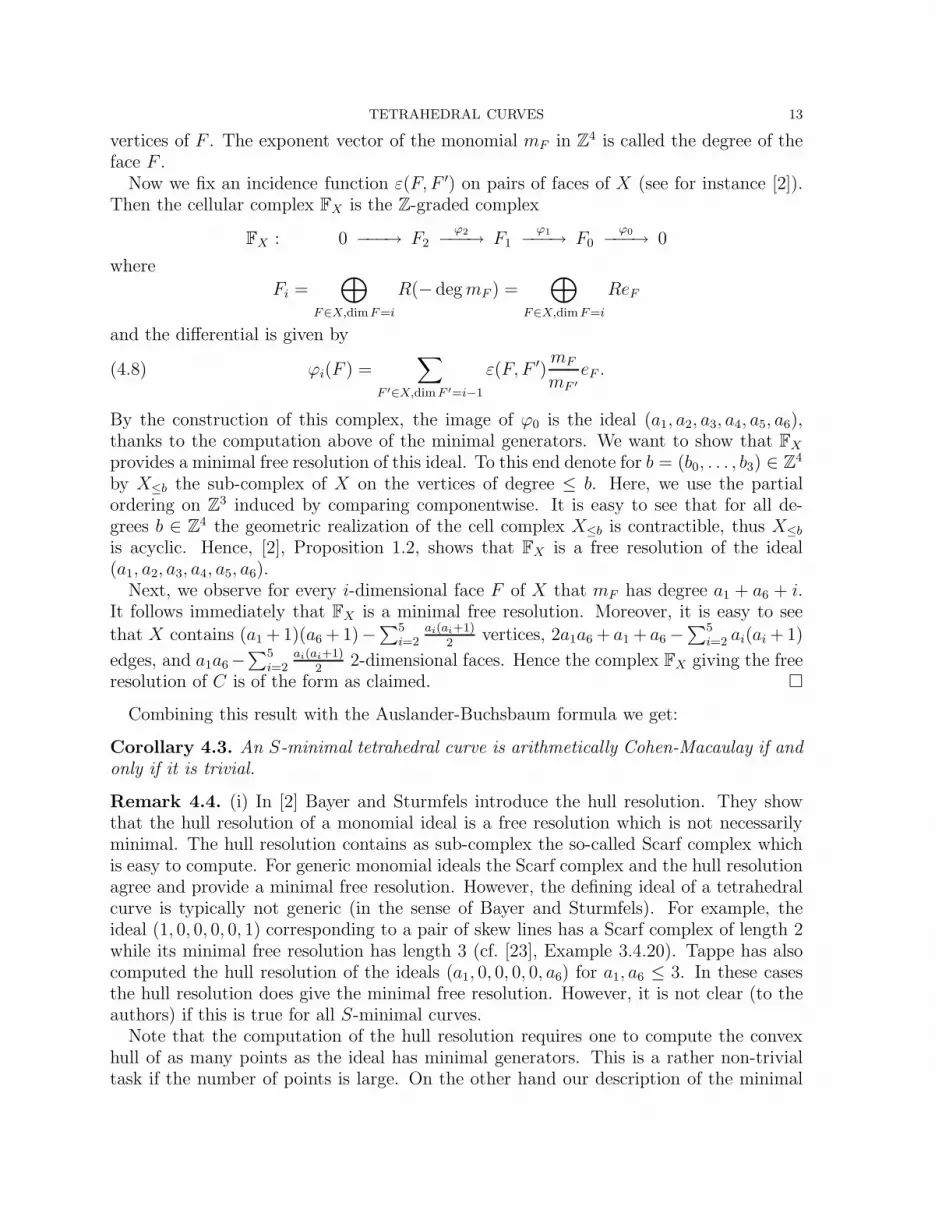
TETRAHEDRAL CURVES 13
vertices of F . The exponent vector of the monomial mF in Z4 is called the degree of the
face F .Now we fix an incidence function ε(F, F ′) on pairs of faces of X (see for instance [2]).
Then the cellular complex FX is the Z-graded complex
FX : 0 −−−→ F2ϕ2
−−−→ F1ϕ1
−−−→ F0ϕ0
−−−→ 0
where
Fi =⊕
F∈X,dimF=i
R(− degmF ) =⊕
F∈X,dimF=i
ReF
and the differential is given by
(4.8) ϕi(F ) =∑
F ′∈X,dimF ′=i−1
ε(F, F ′)mF
mF ′
eF .
By the construction of this complex, the image of ϕ0 is the ideal (a1, a2, a3, a4, a5, a6),thanks to the computation above of the minimal generators. We want to show that FX
provides a minimal free resolution of this ideal. To this end denote for b = (b0, . . . , b3) ∈ Z4
by X≤b the sub-complex of X on the vertices of degree ≤ b. Here, we use the partialordering on Z
3 induced by comparing componentwise. It is easy to see that for all de-grees b ∈ Z
4 the geometric realization of the cell complex X≤b is contractible, thus X≤b
is acyclic. Hence, [2], Proposition 1.2, shows that FX is a free resolution of the ideal(a1, a2, a3, a4, a5, a6).
Next, we observe for every i-dimensional face F of X that mF has degree a1 + a6 + i.It follows immediately that FX is a minimal free resolution. Moreover, it is easy to see
that X contains (a1 + 1)(a6 + 1)−∑5
i=2ai(ai+1)
2vertices, 2a1a6 + a1 + a6 −
∑5i=2 ai(ai + 1)
edges, and a1a6−∑5
i=2ai(ai+1)
22-dimensional faces. Hence the complex FX giving the free
resolution of C is of the form as claimed. �
Combining this result with the Auslander-Buchsbaum formula we get:
Corollary 4.3. An S-minimal tetrahedral curve is arithmetically Cohen-Macaulay if and
only if it is trivial.
Remark 4.4. (i) In [2] Bayer and Sturmfels introduce the hull resolution. They showthat the hull resolution of a monomial ideal is a free resolution which is not necessarilyminimal. The hull resolution contains as sub-complex the so-called Scarf complex whichis easy to compute. For generic monomial ideals the Scarf complex and the hull resolutionagree and provide a minimal free resolution. However, the defining ideal of a tetrahedralcurve is typically not generic (in the sense of Bayer and Sturmfels). For example, theideal (1, 0, 0, 0, 0, 1) corresponding to a pair of skew lines has a Scarf complex of length 2while its minimal free resolution has length 3 (cf. [23], Example 3.4.20). Tappe has alsocomputed the hull resolution of the ideals (a1, 0, 0, 0, 0, a6) for a1, a6 ≤ 3. In these casesthe hull resolution does give the minimal free resolution. However, it is not clear (to theauthors) if this is true for all S-minimal curves.
Note that the computation of the hull resolution requires one to compute the convexhull of as many points as the ideal has minimal generators. This is a rather non-trivialtask if the number of points is large. On the other hand our description of the minimal

14 J. MIGLIORE, U. NAGEL
free resolution of S-minimal curves uses a very simple cell complex which gives a moredirect approach.
(ii) After we had found the cell complex that determines the minimal free resolution ofan S-minimal curve we realized that Schwartau [20] uses a similar description in order tocompute the minimal free resolution of any tetrahedral curve with a2 = a5 = 0. However,much of the theory that we have used here was not available during the writing of [20],and we found that proof to be less “clean” even in the restricted setting.
As another consequence of Theorem 4.2 we get some information about the Hartshorne-Rao module of any tetrahedral curve. Recall that the Hartshorne-Rao module of a curveC is the graded module
M(C) := ⊕j∈ZH1(IC(j)).
Corollary 4.5. The K-dual of the Hartshorne-Rao module of a tetrahedral curve is gen-
erated in one degree.
Proof. Since the Hartshorne-Rao module is up to degree shift invariant in an even liaisonclass, it suffices to show the claim for a non-trivial S-minimal curve C. By local dualitywe have the following graded isomorphism
M(C)∨ ∼= Ext3(R/IC , R)(−4).
The latter module can be computed from the minimal free resolution of IC . Since it islinear the claim follows. �
Remark 4.6. (i) The conclusion of the last result is in general not true for theHartshorne-Rao module itself. Indeed, the Hartshorne-Rao module of the curve(5, 2, 2, 1, 1, 5) has minimal generators in two different degrees, namely 4 and 5.
(ii) The curve in (i) also shows that in general we cannot link a tetrahedral curve in anodd number of steps to a tetrahedral curve.
From a cohomological point of view the simplest curves that are not arithmeticallyCohen-Macaulay are the arithmetically Buchsbaum curves. The tetrahedral curves amongthem have special properties.
Corollary 4.7. A tetrahedral curve is arithmetically Buchsbaum if and only if its
Hartshorne-Rao module satisfies
M(C) ∼= Km(t) for some integers m, t where m ≥ 0.
Proof. This follows immediately by Corollary 4.5. �
Remark 4.8. The fact that such arithmetically Buchsbaum curves exist was knownalready to Schwartau, who constructed them with liaison addition. The fact that theyare the only arithmetically Buchsbaum curves among the tetrahedral curves is new.
5. Minimality in the Even Liaison Class, and Applications
Now we want to show that for tetrahedral curves the concept of S-minimality andminimality in its even liaison class agree. This is the second main result of this paper.
Theorem 5.1. Let C be a tetrahedral curve which is not arithmetically Cohen-Macaulay.
Then C is S-minimal if and only if it is minimal in its even liaison class.
TETRAHEDRAL CURVES 15
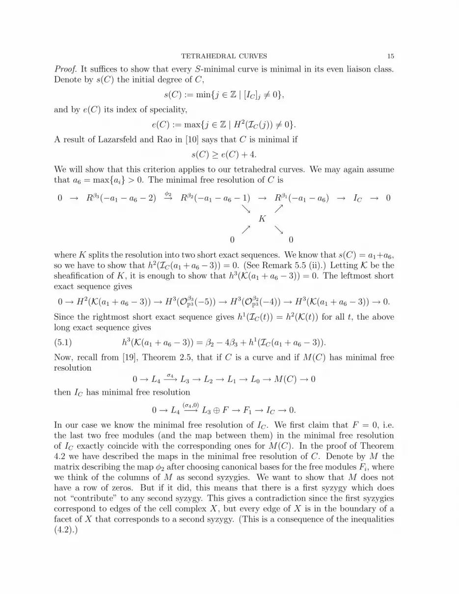
Proof. It suffices to show that every S-minimal curve is minimal in its even liaison class.Denote by s(C) the initial degree of C,
s(C) := min{j ∈ Z | [IC ]j 6= 0},
and by e(C) its index of speciality,
e(C) := max{j ∈ Z | H2(IC(j)) 6= 0}.
A result of Lazarsfeld and Rao in [10] says that C is minimal if
s(C) ≥ e(C) + 4.
We will show that this criterion applies to our tetrahedral curves. We may again assumethat a6 = max{ai} > 0. The minimal free resolution of C is
0 → Rβ3(−a1 − a6 − 2)φ2→ Rβ2(−a1 − a6 − 1) → Rβ1(−a1 − a6) → IC → 0
ց րK
ր ց0 0
whereK splits the resolution into two short exact sequences. We know that s(C) = a1+a6,so we have to show that h2(IC(a1 + a6 − 3)) = 0. (See Remark 5.5 (ii).) Letting K be thesheafification of K, it is enough to show that h3(K(a1 + a6 − 3)) = 0. The leftmost shortexact sequence gives
0 → H2(K(a1 + a6 − 3)) → H3(Oβ3
P3(−5)) → H3(Oβ2
P3(−4)) → H3(K(a1 + a6 − 3)) → 0.
Since the rightmost short exact sequence gives h1(IC(t)) = h2(K(t)) for all t, the abovelong exact sequence gives
(5.1) h3(K(a1 + a6 − 3)) = β2 − 4β3 + h1(IC(a1 + a6 − 3)).
Now, recall from [19], Theorem 2.5, that if C is a curve and if M(C) has minimal freeresolution
0 → L4σ4−→ L3 → L2 → L1 → L0 →M(C) → 0
then IC has minimal free resolution
0 → L4(σ4,0)−→ L3 ⊕ F → F1 → IC → 0.
In our case we know the minimal free resolution of IC . We first claim that F = 0, i.e.the last two free modules (and the map between them) in the minimal free resolutionof IC exactly coincide with the corresponding ones for M(C). In the proof of Theorem4.2 we have described the maps in the minimal free resolution of C. Denote by M thematrix describing the map φ2 after choosing canonical bases for the free modules Fi, wherewe think of the columns of M as second syzygies. We want to show that M does nothave a row of zeros. But if it did, this means that there is a first syzygy which doesnot “contribute” to any second syzygy. This gives a contradiction since the first syzygiescorrespond to edges of the cell complex X, but every edge of X is in the boundary of afacet of X that corresponds to a second syzygy. (This is a consequence of the inequalities(4.2).)

16 J. MIGLIORE, U. NAGEL
Thus we know the end of the minimal free resolution for M(C) has the form
0 → Rβ3(−a1 − a6 − 2)φ2
−→ Rβ2(−a1 − a6 − 1) → . . . ,
and as a result the minimal free resolution for the dual module (over the field K) M(C)∨
has the form
· · · → F → Rβ2(a1 + a6 − 3)φ∨
2−→ Rβ3(a1 + a6 − 2) →M(C)∨ → 0.
It is a basic property of minimal free resolutions that F has no summand of the formR(a1 +a6−3). Hence dimM(C)∨−a1−a6+3 = 4β3−β2, so (5.1) gives h3(K(a1 +a6−3)) = 0as desired. �
Corollary 5.2. Assume that a6 = max{a1, . . . , a6}. Then the degree of an S-minimal
curve of type (a1, . . . , a6) is∑6
i=1
(ai+1
2
), and the arithmetic genus is
[6∑
i=1
(ai + 1
2
)]
(a1 + a6 − 1) + 1 −
(a1 + a6 + 2
3
)
.
Proof. The degree statement is obvious. As for the arithmetic genus, let us denote it byg. It follows easily from the calculations in the proof of Theorem 5.1 that
h0(IC(a1 + a6 − 1)) = h1(IC(a1 + a6 − 1)) = h2(IC(a1 + a2 − 1)) = 0.
From the cohomology of the exact sequence
0 → IC → OP3 → OC → 0
(twisted by a1 + a6 − 1) it follows that
h0(OC(a1 + a6 − 1)) =
(a1 + a6 + 2
3
)
.
We also have h1(OC(t)) = h2(IC(t)) for all t. But the Riemann-Roch theorem gives that
h0(OC(a1 + a6 − 1)) = (degC)(a1 + a6 − 1) − g + 1 + h1(OC(a1 + a6 − 1)).
Combining the above calculations gives the result. �
The following theorem can be viewed as a clarification of Schwartau’s theorem (seeTheorem 2.4 and Remark 2.5) and its proof is new and uses the methods of our paper.The main tool is Lemma 3.8, but we have put it after Theorem 5.1 because we use thefact that an S-minimal curve is not ACM, and this follows from the fact that a curve thatis minimal in its even liaison class is not ACM.
Theorem 5.3 (invariant Schwartau). The ideal
(a, b)a1 ∩ (a, c)0 ∩ (a, d)a3 ∩ (b, c)a4 ∩ (b, d)0 ∩ (c, d)a6
defines an arithmetically Cohen-Macaulay curve in P3 if and only if
Case 1. a1, a3, a4, a6 > 0: a1 + a6 = a3 + a4 + ǫ, where ǫ ∈ {−1, 0, 1}.
Case 2. Exactly one of a1, a3, a4, a6 is zero, say ai: a7−i + 1 ≥ the sum of the weights of
the lines meeting the line li.

TETRAHEDRAL CURVES 17
Case 3. At least two of a1, a3, a4, a6 are zero: the curve is connected.
Proof. For convenience we will call a curve of the form given in Theorem 5.3 a Schwartau
curve. If C is a Schwartau curve then its components can be represented by a square:
a1
a3 a4
a6
If three of the integers ai are zero then the ideal is a power of a complete intersection, andis automatically ACM and connected. Suppose that two of the integers ai are zero. If Cis ACM then it is a general fact that it must be connected. Conversely, suppose that C isconnected. This means that the two non-zero values of ai represent adjacent sides of thesquare. Hence the ideal involves only three variables. The fourth variable is thus a nonzero-divisor, and reducing modulo this variable gives the saturated ideal of a zeroschemein P
2. Hence in this case the Schwartau curve is ACM. This proves Case 3.Now suppose that one of the integers is zero, say ai. (Note that Schwartau took a3 = 0.)
As long as C is not S-minimal, we can reduce any maximal facet, by Lemma 3.8. Butwith ai = 0, there remain only two facets, whose weights are the sums of two consecutivesides of the square. (For example, if a3 = 0 then the weights of the facets are a4 + a6 anda1 + a4.)
If C is ACM then no reduction will ever be S-minimal. We repeatedly reduce the facetof maximal weight until we obtain another zero for the weight of an edge, and the factthat C is ACM means that after obtaining this zero, the remaining two edges must beconnected (by Case 3 above). This means that the “middle” of the three non-zero edges,a7−i, must not be the first to reach 0 unless there is a tie. But this middle edge is involvedin every reduction! Note that since we are always reducing the facet of maximal weight,we eventually reach the point where the weights of the non-middle edges differ by at most1. It follows that a7−i + 1 ≥ the sum of the weights of the two “non-middle” edges, asclaimed.
Conversely, suppose that a7−i + 1 ≥ the sum of the weights of the two “non-middle”edges. Then clearly a7−i is the edge of maximal weight. The condition (b) of Lemma 3.8is trivial to check, so C is not minimal and we can reduce the facet of maximal weight.In doing so, both sides of the inequality in Case 2 are reduced by 1, so the inequality stillholds for the new curve. Again, reducing the facet of maximal weight each time eventuallyleads to a balance in the two non-middle edges, and the given inequality guarantees thatthe curve resulting when a second 0 is obtained, will be connected, hence ACM. So C isACM.
We now consider the case where none of the ai are 0. Again without loss of gener-ality assume that a6 = max{a1, a3, a4, a6}. One can check that then w = max{a3 + a6,a4 +a6}. It follows that when we reduce a facet of maximal weight (if it is possible), we si-multaneously reduce max{a1, a6} and max{a3, a4} by 1. In particular, we simultaneouslyreduce (a1 + a6) by 1 and (a3 + a4) by 1.
18 J. MIGLIORE, U. NAGEL
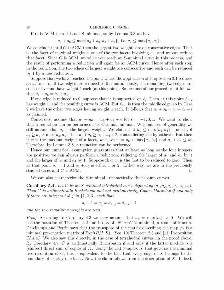
If C is ACM then it is not S-minimal, so by Lemma 3.8 we have
a1 + a6 ≤ max{a3 + a6, a4 + a6}, i.e. a1 ≤ max{a3, a4}.
We conclude that if C is ACM then the largest two weights are on consecutive edges. Thatis, the facet of maximal weight is one of the two facets involving a6, and we can reducethat facet. Since C is ACM, we will never reach an S-minimal curve in this process, andthe result of performing a reduction will again be an ACM curve. Hence after each stepin the reduction, the two edges of largest weight are consecutive and each can be reducedby 1 by a new reduction.
Suppose that we have reached the point where the application of Proposition 3.1 reducesan ai to zero. If two edges are reduced to 0 simultaneously, the remaining two edges areconsecutive and have weight 1 each (at this point). So because of our procedure, it followsthat a1 + a6 = a3 + a4.
If one edge is reduced to 0, suppose that it is supported on ℓi. Then at this point ℓ7−ihas weight 1, and the resulting curve is ACM. But ℓ7−i is then the middle edge, so by Case2 we have the other two edges having weight 1 each. It follows that a1 + a6 = a3 + a4 + ǫas claimed.
Conversely, assume that a1 + a6 = a3 + a4 + ǫ for ǫ = −1, 0, 1. We want to showthat a reduction can be performed, i.e. C is not minimal. Without loss of generality westill assume that a6 is the largest weight. We claim that a1 ≤ max{a3, a4}. Indeed, ifa6 ≥ a1 > max{a3, a4} then a1 + a6 ≥ a3 + a4 +2, contradicting the hypothesis. But thenif w is the maximal weight of a facet, we have w = a6 + max{a3, a4} and a1 + a6 ≤ w.Therefore, by Lemma 3.8, a reduction can be performed.
Hence our numerical assumption guarantees that at least as long as the four integersare positive, we can always perform a reduction, reducing the larger of a1 and a6 by 1and the larger of a3 and a4 by 1. Suppose that a3 is the first to be reduced to zero. Thenat that point a4 = 1 and a1 + a6 is either 1 or 2. Either way, we are in the previouslystudied cases and C is ACM. �
We can also characterize the S-minimal arithmetically Buchsbaum curves.
Corollary 5.4. Let C be an S-minimal tetrahedral curve defined by (a1, a2, a3, a4, a5, a6).Then C is arithmetically Buchsbaum and not arithmetically Cohen-Macaulay if and only
if there are integers i 6= j in {1, 2, 3} such that
ai + 1 = aj = a7−j = a7−i + 1
and the two remaining weights are zero.
Proof. According to Corollary 4.3 we may assume that a6 = max{ai} > 0. We willuse the notation of Theorem 4.2 and its proof. Since C is minimal, a result of Martin-Deschamps and Perrin says that the transpose of the matrix describing the map ϕ2 is aminimal presentation matrix of Ext3(R/I,R). (See [19] Theorem 2.5 and [11] PropositionIV.4.4.) We also saw this directly, in the case of tetrahedral curves, in the proof above.By Corollary 4.7, C is arithmetically Buchsbaum if and only if the latter module is a(shifted) direct sum of copies of K. Using the cell complex X that governs the minimalfree resolution of C, this is equivalent to the fact that every edge of X belongs to theboundary of exactly one facet. Now the claim follows from the description of X. Indeed,
TETRAHEDRAL CURVES 19
after removing diagonals from the corners of (4.1) and translating to the notation of thecell complex X, we must be left with a diagonal of facets and no additional edges, andthis can only happen if we only remove diagonals from two opposite corners of (4.1) inthe prescribed way. �
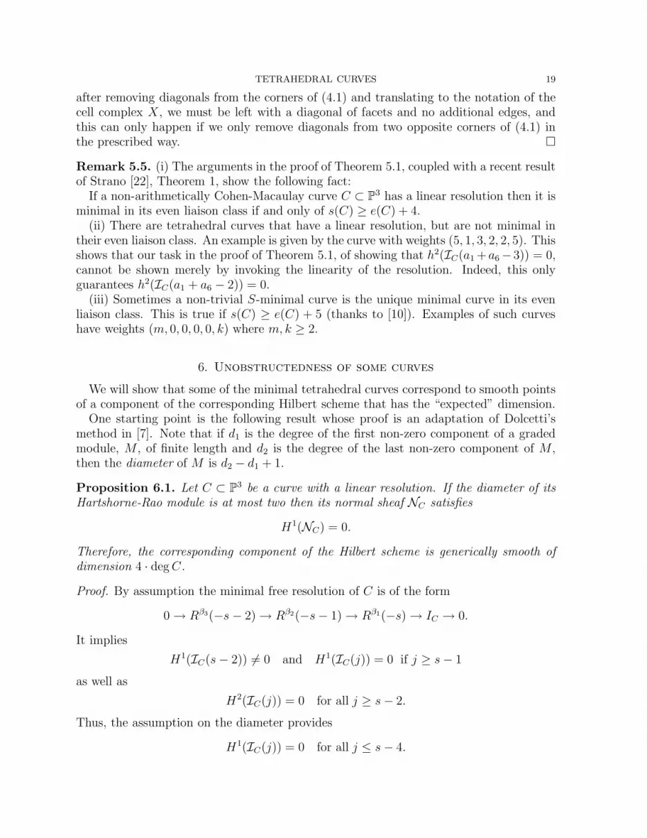
Remark 5.5. (i) The arguments in the proof of Theorem 5.1, coupled with a recent resultof Strano [22], Theorem 1, show the following fact:
If a non-arithmetically Cohen-Macaulay curve C ⊂ P3 has a linear resolution then it is
minimal in its even liaison class if and only of s(C) ≥ e(C) + 4.(ii) There are tetrahedral curves that have a linear resolution, but are not minimal in
their even liaison class. An example is given by the curve with weights (5, 1, 3, 2, 2, 5). Thisshows that our task in the proof of Theorem 5.1, of showing that h2(IC(a1 +a6 −3)) = 0,cannot be shown merely by invoking the linearity of the resolution. Indeed, this onlyguarantees h2(IC(a1 + a6 − 2)) = 0.
(iii) Sometimes a non-trivial S-minimal curve is the unique minimal curve in its evenliaison class. This is true if s(C) ≥ e(C) + 5 (thanks to [10]). Examples of such curveshave weights (m, 0, 0, 0, 0, k) where m, k ≥ 2.
6. Unobstructedness of some curves
We will show that some of the minimal tetrahedral curves correspond to smooth pointsof a component of the corresponding Hilbert scheme that has the “expected” dimension.
One starting point is the following result whose proof is an adaptation of Dolcetti’smethod in [7]. Note that if d1 is the degree of the first non-zero component of a gradedmodule, M , of finite length and d2 is the degree of the last non-zero component of M ,then the diameter of M is d2 − d1 + 1.
Proposition 6.1. Let C ⊂ P3 be a curve with a linear resolution. If the diameter of its
Hartshorne-Rao module is at most two then its normal sheaf NC satisfies
H1(NC) = 0.
Therefore, the corresponding component of the Hilbert scheme is generically smooth of
dimension 4 · degC.
Proof. By assumption the minimal free resolution of C is of the form
0 → Rβ3(−s− 2) → Rβ2(−s− 1) → Rβ1(−s) → IC → 0.
It implies
H1(IC(s− 2)) 6= 0 and H1(IC(j)) = 0 if j ≥ s− 1
as well as
H2(IC(j)) = 0 for all j ≥ s− 2.
Thus, the assumption on the diameter provides
H1(IC(j)) = 0 for all j ≤ s− 4.
20 J. MIGLIORE, U. NAGEL
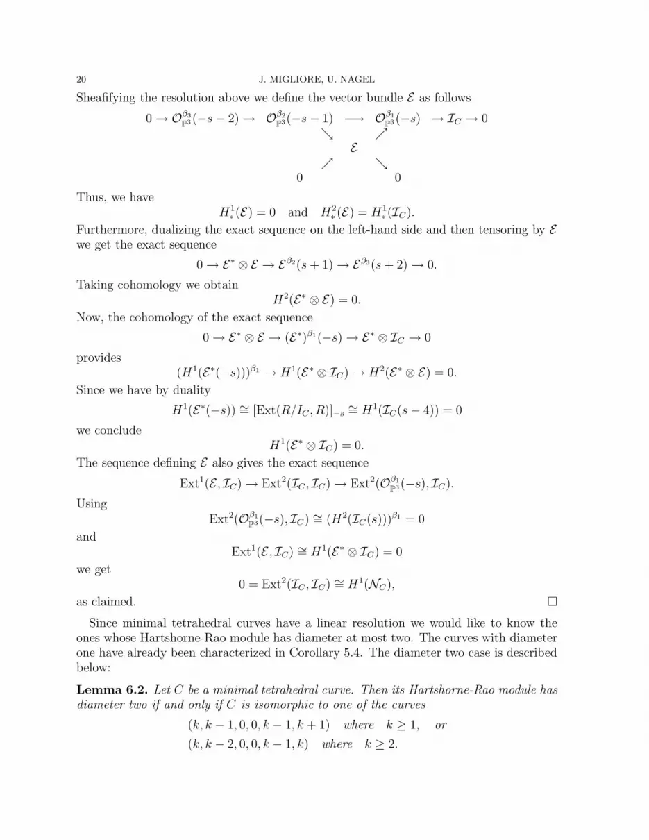
Sheafifying the resolution above we define the vector bundle E as follows
0 → Oβ3
P3(−s− 2) → Oβ2
P3(−s− 1) −→ Oβ1
P3(−s) → IC → 0ց ր
Eր ց
0 0
Thus, we haveH1
∗ (E) = 0 and H2∗ (E) = H1
∗ (IC).
Furthermore, dualizing the exact sequence on the left-hand side and then tensoring by Ewe get the exact sequence
0 → E∗ ⊗ E → Eβ2(s+ 1) → Eβ3(s+ 2) → 0.
Taking cohomology we obtainH2(E∗ ⊗ E) = 0.
Now, the cohomology of the exact sequence
0 → E∗ ⊗ E → (E∗)β1(−s) → E∗ ⊗ IC → 0
provides(H1(E∗(−s)))β1 → H1(E∗ ⊗ IC) → H2(E∗ ⊗ E) = 0.
Since we have by duality
H1(E∗(−s)) ∼= [Ext(R/IC , R)]−s ∼= H1(IC(s− 4)) = 0
we concludeH1(E∗ ⊗ IC) = 0.
The sequence defining E also gives the exact sequence
Ext1(E , IC) → Ext2(IC , IC) → Ext2(Oβ1
P3(−s), IC).
UsingExt2(Oβ1
P3(−s), IC) ∼= (H2(IC(s)))β1 = 0
andExt1(E , IC) ∼= H1(E∗ ⊗ IC) = 0
we get0 = Ext2(IC , IC) ∼= H1(NC),
as claimed. �
Since minimal tetrahedral curves have a linear resolution we would like to know theones whose Hartshorne-Rao module has diameter at most two. The curves with diameterone have already been characterized in Corollary 5.4. The diameter two case is describedbelow:
Lemma 6.2. Let C be a minimal tetrahedral curve. Then its Hartshorne-Rao module has
diameter two if and only if C is isomorphic to one of the curves
(k, k − 1, 0, 0, k − 1, k + 1) where k ≥ 1, or
(k, k − 2, 0, 0, k − 1, k) where k ≥ 2.

TETRAHEDRAL CURVES 21
Proof. Let C be the minimal curve defined by the tuple (a1, a2, a3, a4, a5, a6). Withoutloss of generality assume that a6 is the largest entry. We will use the description of theminimal free resolution of C given in Theorem 4.2. Denote by ψ the dual of the last mapin this resolution, i.e. ψ = ϕ∗
2. Thus, we have the minimal presentation
−−−→ Rβ3(a1 + a6 + 1)ψ
−−−→ Rβ2(a1 + a6 + 2) −−−→ Ext3(R/IC , R) −−−→ 0
Since Ext3(R/IC , R) is the K-dual of the Hartshorne-Rao module MC of C, the diameterof the latter is at most two if and only if
(6.1) [Ext3(R/IC , R)]−a1−a6 = 0.
Denote by X := X(a1, a2, a3, a4, a5, a6) the cell complex of the curve C. Recall fromthe proof of Theorem 4.2 that the facets of X correspond to minimal generators ofExt3(R/IC , R) and that imψ has a system of minimal generators consisting of bino-mials and monomials (cf. formula (4.8)). These generators correspond to the edges of X.Below, we will always refer to this system of generators. Moreover, we will use Diagram(4.7).
We begin with deriving necessary conditions for Condition (6.1) being true. In orderto rule out curves we show two claims.
Claim 1: If X contains “3 facets in a row” then the diameter of MC is greater thantwo.
Here the assumption means that X contains a subcomplex that is isomorphic toX(3, 0, 0, 0, 0, 1) (a “vertical row”) or X(1, 0, 0, 0, 0, 3) (a “horizontal row”).
Now, assume that X contains 3 facets in a horizontal row. Denote by e1, e2, e3 thesefacets from left to right. Then, the only minimal generators of imψ involving ce1, ce2, de2,or de3 are (up to sign)
−ce1 + de2 and − ce2 + de3.
It follows easily that all the monomials c2e1, cde2, d2e3 do not belong to imψ. Thus,
condition (6.1) is not satisfied.If X contains 3 facets in a vertical row we argue similarly and Claim 1 is shown.Claim 2: If X contains a “square of 4 facets” then the diameter of MC is greater than
two.More precisely, the assumption means that X contains a subcomplex that is isomor-
phic to X(2, 0, 0, 0, 0, 2). Enumerate its facets counterclockwise by e1, . . . , e4 beginningwith e1 in the “Southwest” corner. Then, the only minimal generators of imψ involvingbe1, ce1, be2, de2, ae3, de3, ae4, or ce4 are (up to sign)
− ce1 + de2, −be2 + ae3
− ce4 + de3, −be1 + ae4.
Hence, all the monomials bce1, bde2, ade3, ace4 are not in imψ. Thus, condition (6.1) isnot satisfied and Claim 2 is established.
As the next step we look for the minimal tetrahedral curves whose cell complex containsneither 3 facets in a row nor a square of 4 facets. Let C be such a curve. Looking at the

22 J. MIGLIORE, U. NAGEL
boundaries of its cell complex X we get in conjunction with Corollary 3.5
1 ≤ a6 − a4 − a5 ≤ 2
1 ≤ a6 − a2 − a3 ≤ 2
1 ≤ a1 − a3 − a5 ≤ 2
1 ≤ a1 − a2 − a4 ≤ 2.
Now, we look at a horizontal or vertical boundary of X a bit more carefully. If there aretrue “cuts” on both ends then the row ofX next to it has length at least 3, a contradiction.Thus, we may assume without loss of generality that
a3 = 0.
Next, we distinguish two cases.Case 1: Assume a2 = 0. Then we get a6 ≤ 2 and it is easy to see that C can be any
curve satisfying these conditions except the curve defined by (2, 0, 0, 0, 0, 2).Case 2: Assume a2 > 0. Using the argument above for the Eastern boundary of X we
conclude
a4 = 0.
We are left with two possibilities for the value of a5.Case 2.1: Assume a5 = a6 − 1. Since a5 < a1 ≤ a6 we obtain a1 = a6. We conclude
that either a2 = a6 − 1, i.e. C is an arithmetically Buchsbaum curve of type
(k, k − 1, 0, 0, k − 1, k),
or a2 = a6 − 2, i.e. C is of type
(k, k − 2, 0, 0, k − 1, k).
Case 2.2: Assume a5 = a6 − 2. Since the length of the row next to the Northernboundary of X is at most 3 we get a2 = a1 − 1. It follows that either a1 = a6, i.e. C isisomorphic to the second kind of curve in Case 2.1, or a1 = a6 − 1, i.e. C is of type
(k, k − 1, 0, 0, k − 1, k + 1).
Summing up. we have shown that there are at most three types of minimal tetrahedralcurves satisfying Condition (6.1). Since we already know all the curves with diameter one(by Corollary 4.7), it remains to show that the diameter of the curves specified in thestatement is at most two.
Let C be the curve defined by
(k, k − 1, 0, 0, k − 1, k + 1).
Enumerate the facets of the cell complex X of C by e1, . . . , e2k such that e1 is the facet inthe Southeast corner and the facets ei and ei+1 are neighbours. This enumeration existsand is uniquely determined due to the shape of X. We will show that
(6.2) (a, b, c, d)2 · ei ∈ imψ for all i = 1, . . . , 2k.
First, we consider e1. Since (a, b, d) · e1 ∈ imψ it suffices to show c2e1 ∈ imψ. But thisfollows easily using
c · (−ce1 + de2) ∈ imψ

TETRAHEDRAL CURVES 23
andce2 ∈ imψ.
Next, we consider e2. Since also ae2 ∈ imψ it remains to show (b, d)2 · e2 ∈ imψ. Usingthe minimal generators −ce1 + de2, be1, de1 we see that
(bd, d2)e2 ∈ imψ.
We also haveb2e2 ∈ imψ
because −be2 + ae3, be3 ∈ imψ.Continuing similarly in this fashion we can show the relations (6.2) that imply Condition
(6.1). This completes the argument. �
Corollary 6.3. Let C be a curve that is isomorphic to one of the curves
(k, k − 1, 0, 0, k − 1, k) where k ≥ 1,
(k, k − 1, 0, 0, k − 1, k + 1) where k ≥ 1, or
(k, k − 2, 0, 0, k − 1, k) where k ≥ 2.
Then C is unobstructed and the corresponding component of the Hilbert scheme is gener-
ically smooth and has dimension 4 · degC.
Proof. This follows by combining Proposition 6.1, Lemma 6.2, and Theorem 4.2. �
Remark 6.4. It was proved in [4] that if C is a curve in P3 (not necessarily tetrahedral)
with natural cohomology and if the diameter ofM(C) is two, then C is unobstructed and itsHilbert scheme has the expected dimension. “Natural cohomology” means that for any t,no two of h0(IC(t)), h1(IC(t)) and h2(IC(t)) are non-zero. Note that minimal tetrahedralcurves whose Hartshorne-Rao modules have diameter two have natural cohomology.
Note also that our Proposition 6.1, while similar, is independent of that result. Forexample, a non-minimal tetrahedral curve with linear resolution (e.g. (6, 5, 1, 0, 4, 6)) doesnot have natural cohomology, but is unobstructed by Proposition 6.1. On the other hand,a minimal arithmetically Buchsbaum curve C with M(C) of diameter two does not havea linear resolution (since the dual module would then be generated in more than onedegree), but it does have natural cohomology (cf. [3], for instance Corollary 2.5 with t = 2and h = 0) and so is unobstructed.
We also remark that Miro-Roig has given sufficient conditions on the numerical char-acter of an irreducible arithmetically Buchsbaum curve C of maximal rank with M(C) ofdiameter one or two, for C to be unobstructed (cf. [17]).
The condition on the diameter of the minimal tetrahedral curves in Proposition 6.1 issufficient for unobstructedness, but not necessary. This is shown by the curves(a1, 0, 0, 0, 0, a6) because their diameter is a1 + a6 − 1, but all these curves are unob-structed. This follows from the following result.
Proposition 6.5. The global sections of the normal sheaf of the curve C defined by
(a1, 0, 0, 0, 0, a6) are given by
H0∗ (NC) ∼= (R/(a, b))a1(a1+1)(1) ⊕ (R/(c, d))a6(a6+1)(1).
24 J. MIGLIORE, U. NAGEL
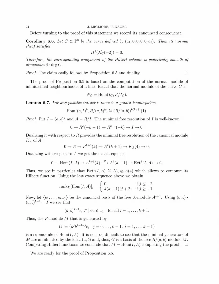
Before turning to the proof of this statement we record its announced consequence.
Corollary 6.6. Let C ⊂ P3 be the curve defined by (a1, 0, 0, 0, 0, a6). Then its normal
sheaf satisfies
H1(NC(−2)) = 0.
Therefore, the corresponding component of the Hilbert scheme is generically smooth of
dimension 4 · degC.
Proof. The claim easily follows by Proposition 6.5 and duality. �
The proof of Proposition 6.5 is based on the computation of the normal module ofinfinitesimal neighbourhoods of a line. Recall that the normal module of the curve C is
NC = Hom(IC , R/IC).
Lemma 6.7. For any positive integer k there is a graded isomorphism
Hom((a, b)k, R/(a, b)k) ∼= (R/(a, b))k(k+1)(1).
Proof. Put I = (a, b)k and A = R/I. The minimal free resolution of I is well-known
0 → Rk(−k − 1) → Rk+1(−k) → I → 0.
Dualizing it with respect to R provides the minimal free resolution of the canonical moduleKA of A
0 → R→ Rk+1(k) → Rk(k + 1) → KA(4) → 0.
Dualizing with respect to A we get the exact sequence
0 → Hom(I, A) → Ak+1(k)ψ
−→ Ak(k + 1) → Ext1(I, A) → 0.
Thus, we see in particular that Ext1(I, A) ∼= KA ⊗ A(4) which allows to compute itsHilbert function. Using the last exact sequence above we obtain
rankK [Hom(I, A)]j =
{0 if j ≤ −2k(k + 1)(j + 2) if j ≥ −1
Now, let {e1, . . . , ek+1} be the canonical basis of the free A-module Ak+1. Using (a, b) ·(a, b)k−1 = I we see that
(a, b)k−1ei ⊂ [kerψ]−1 for all i = 1, . . . , k + 1.
Thus, the R-module M that is generated by
G := {ajbk−1−jei | j = 0, . . . , k − 1, i = 1, . . . , k + 1}
is a submodule of Hom(I, A). It is not too difficult to see that the minimal generators ofM are annihilated by the ideal (a, b) and, thus, G is a basis of the free R/(a, b)-module M .Comparing Hilbert functions we conclude that M = Hom(I, A) completing the proof. �
We are ready for the proof of Proposition 6.5.

TETRAHEDRAL CURVES 25
Proof of Proposition 6.5. Let C1, C2 be the curves defined by (a, b)a1 and (c, d)a6 , respec-tively. Using the exact sequence
0 → IC → IC1⊕ IC2
→ IC1+ IC2
→ 0
we get
H0∗ (OC) ∼= H0
∗ (OC1) ⊕H0
∗ (OC2).
Since H0∗ (NC) ∼= Hom(IC , H
0∗ (OC)) it is not too difficult to see that the claim follows by
Lemma 6.7. �
7. Remarks and problems
In this section we collect some observations that do not quite fit into earlier sectionsof this paper, as well as some natural questions that arise from this work. The list ofquestions is rather long, highlighting the richness of this line of inquiry. The authors planto continue investigating these questions.
Remark 7.1. It is natural to ask, among all tetrahedral curves, “how many” are minimalin their even liaison class. That is, can we describe the density of minimal tetrahedralcurves among all tetrahedral curves? The first answer is “almost none,” since of courseevery such even liaison class has infinitely many tetrahedral curves, but essentially oneminimal one (but see question 1. below). But paradoxically, we can take a different pointof view that shows that there are more than one might think.
We want to investigate how many minimal tetrahedral curves are in a finite set oftetrahedral curves. To this end it seems reasonable to fix the maximum entry of the 6-tuple. After a change of coordinates we may assume that this entry is the last one. Thenwe get:
Lemma 7.2. The number of minimal tetrahedral curves (a1, . . . , a6) such that a6 =max{a1, . . . , a6} is
N(a6) :=
a6∑
a1=0
a1−1∑
a2=0
a1−1∑
a5=0
min{a1 − a5, a6 − a2} · min{a1 − a2, a6 − a5}.
Proof. This is a consequence of Corollary 3.5. If (a1, . . . , a6) is minimal then we have0 ≤ a1 ≤ a6 and 0 ≤ a2, a5 < a1. Moreover, having chosen a1, a2, a5, the only conditionfor a3 and a4 is 0 ≤ a3 < min{a1 − a5, a6 − a2} and 0 ≤ a4 < min{a1 − a2, a6 − a5},respectively. The claim follows. �
The number of tetrahedral curves with fixed a6 = max{a1, . . . , a6} is (a6 + 1)5. Thelemma shows that the number of minimal curves among them is also of order a5
6. To seethis it suffices to find a lower estimate of the number N(a6). Since both minima in the

26 J. MIGLIORE, U. NAGEL
formula in Lemma 7.2 are at least a1 − min{a2, a5} we get
N(a6) ≥a6∑
a1=0
a1−1∑
a2=0
a1−1∑
a5=0
[a1 − min{a2, a5}]2
=a6∑
a1=0
a1−1∑
a2=0
[a2−1∑
a5=0
(a1 − a5)2 +
a1−1∑
a5=a2
(a1 − a2)2
]
=
a6∑
a1=0
a1−1∑
a2=0
[a1∑
k=a1−a2+1
k2 + (a1 − a2)3
]
Now it is easy to see that this lower estimate of N(a6) is a polynomial in a6 of order 5.In other words, we get the somewhat surprising result: The probability to find a minimalcurve among the set of tetrahedral curves (a1, . . . , a6) such that a6 = max{a1, . . . , a6} ispositive, even as a6 → ∞.
Remark 7.3. The results in this paper can be extended as follows. Let (F1, F2, F3, F4)be a regular sequence. Define curves by IC1
= (F1, F2), IC2= (F1, F3), . . . , IC6
= (F3, F4),and let IC = IC1
∩ · · · ∩ IC6. Taking (F1, F2, F3, F4) = (a, b, c, d) gives the context of this
paper. As before, we denote by (a1, a2, a3, a4, a5, a6) the ideal IC . Note that no two of thecurves Ci can have a common component.
Many of our results extend to this situation. The key observation is that we still have
Fi · (Fi, Fj)n−1 + (F n
j ) = (Fi, Fj)n,
as we noted at the beginning of the proof of Proposition 3.1. Then Proposition 3.1 andCorollary 3.5 (and indeed virtually all of section 3) are still true, as stated, in this moregeneral context. Turning to Section 4, Theorem 4.2 is clearly not true as stated. If the Fiall have the same degree, it is fairly easy to modify the statement, and in fact the linearityof the resolution is preserved. If the Fi have different degrees, it can still be modified,but the resolution is no longer linear. The other results are less obviously generalizableto this context.
We end with some open questions.
Question 7.4. (1) Fix an even liaison class containing tetrahedral curves. We knowthat among the minimal curves there is at least one that is tetrahedral. When is aminimal tetrahedral curve the unique minimal curve in the even liaison class (seeRemark 5.5, (iii))? Note that sometimes two curves that are projectively equiva-lent are linked, and sometimes they are not!
(2) Is it possible to characterize the tetrahedral curves with linear resolutions? Recallthat this set of curves contains more than just the minimal tetrahedral curves(Remark 5.5 (ii)).
(3) We have seen that several of the minimal tetrahedral curves are unobstructed.Computer experiments show that there are more of them than the ones describedabove. Are all minimal tetrahedral curves unobstructed? Are all tetrahedral
TETRAHEDRAL CURVES 27
curves with linear resolution unobstructed? Are all tetrahedral curves unob-structed?
(4) How “dense” are our minimal curves that give rise to nice components of theHilbert scheme Hd,g, i.e. components that are generically smooth of dimension 4d?In other words: How big are the “gaps” in the sets of pairs (d, g) such we cannotfind such a minimal curve with that degree and genus?
(5) Can the tetrahedral curves in P3 that are arithmetically Cohen-Macaulay be iden-
tified by explicitly giving the 6-tuples (as Schwartau does for 4-tuples)?
(6) Is there a combinatorial description of the minimal free resolution of the deficiencymodule of a tetrahedral curve? Can we at least express the dimensions of the com-ponents using the entries of the 6-tuple?
(7) Can the same kind of program be carried out in higher projective space? Now thenew question of local Cohen-Macaulayness arises. This includes codimension twocases and higher codimension cases. The former can still rely on complete inter-section liaison techniques, but the latter will require Gorenstein liaison techniques.
(8) On a computer algebra program such as macaulay [1] one can make experiments,and one notices a great deal of structure in the Betti diagram. In particular, non-minimal tetrahedral curves have linear strands in the resolution. How do thesearise? Certainly they come from the Betti diagram of the minimal tetrahedralcurve using basic double links, but this should be explained in a clearer way. Canone relate the “degree of non-minimality” to the number of linear strands? Theresult of [16] Corollary 4.5 should be useful.
(9) Is it possible to use similar techniques to study more general monomial ideals?
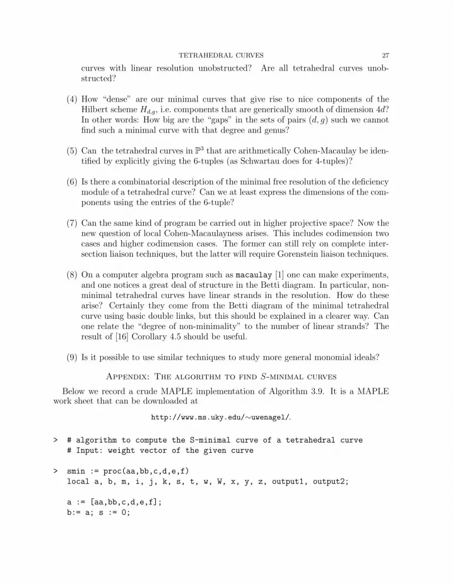
Appendix: The algorithm to find S-minimal curves
Below we record a crude MAPLE implementation of Algorithm 3.9. It is a MAPLEwork sheet that can be downloaded at
http://www.ms.uky.edu/∼uwenagel/.
> # algorithm to compute the S-minimal curve of a tetrahedral curve
# Input: weight vector of the given curve
> smin := proc(aa,bb,c,d,e,f)
local a, b, m, i, j, k, s, t, w, W, x, y, z, output1, output2;
a := [aa,bb,c,d,e,f];
b:= a; s := 0;

28 J. MIGLIORE, U. NAGEL
if (s > -1) then do
# 1. computation of the maximal weight m of a line
m := a[1]; j := 1;
for i from 2 to 6 do
if (a[i] > m) then m := a[i];
j := i;
end if;
od;
# 2. avoid unnecessary computations
if (m = 0) then
output1 := matrix(1,6,[[‘ ‘,‘Minimal curve to‘, b, ‘is‘, a,‘ ‘]]):
output2:= matrix(1,3,[[‘It is obtained after‘, s,‘ reduction(s).‘]]):
print(output1); print(output2);
return(a);
end if;
# 3. computation of facet of maximal weight W
x := a[1] + a[2] + a[3];
y := a[1] + a[4] + a[5];
z := a[2] + a[4] + a[6];
t := a[3] + a[5] + a[6];
w := [x, y, z, t];
W:= w[1]; k := 1;
for i from 2 to 4 do
if (w[i] > W) then W := w[i];
k := i;
end if;
od;
# 4. test if curve is S-minimal
if (a[j] + a[7-j] > W) then
output1 := matrix(1,6,[[‘ ‘,‘Minimal curve to‘, b, ‘is‘, a,‘ ‘]]):
output2:= matrix(1,3,[[‘It is obtained after‘, s,‘ reduction(s).‘]]):
print(output1); print(output2);
return(a);
end if;
# 5. reduction of the non-minimal curve

TETRAHEDRAL CURVES 29
s := s+1;
if (k = 1) then a[1] := max(0, a[1] - 1);
a[2] := max(0, a[2] - 1);
a[3] := max(0, a[3] - 1);
end if;
if (k = 2) then a[1] := max(0, a[1] - 1);
a[4] := max(0, a[4] - 1);
a[5] := max(0, a[5] - 1);
end if;
if (k = 3) then a[2] := max(0, a[2] - 1);
a[4] := max(0, a[4] - 1);
a[6] := max(0, a[6] - 1);
end if;
if (k = 4) then a[3] := max(0, a[3] - 1);
a[5] := max(0, a[5] - 1);
a[6] := max(0, a[6] - 1);
end if;
end do;
end if;
end:
In order to use the procedure above in a different work sheet one could write it into atext file named, for example, proc.txt. Then it can be used as follows.
> read ‘C:\\suitable path\\proc.txt‘;
> smin(5,1,3,2,2,5):
[ , Minimal curve to , [5, 1, 3, 2, 2, 5] , is ,
[5, 1, 2, 2, 1, 4] , ]

30 J. MIGLIORE, U. NAGEL
[It is obtained after 1 reduction(s).]
> smin(6,0,8,1,0,4):
[ , Minimal curve to , [6, 0, 8, 1, 0, 4] , is ,
[0, 0, 0, 0, 0, 0] , ]
[It is obtained after 10 reduction(s).]
References
[1] D. Bayer and M. Stillman, Macaulay: A system for computation in algebraic geometry and com-mutative algebra. Source and object code available for Unix and Macintosh computers. Contact theauthors, or download from ftp://math.harvard.edu via anonymous ftp.
[2] D. Bayer and B. Sturmfels, Cellular resolutions of monomial modules, J. Reine Angew. Math. 502(1998), 123–140.
[3] G. Bolondi and J. Migliore, Buchsbaum Liaison Classes, J. Algebra 123 (1989), 426–456.[4] G. Bolondi and J. Migliore, On curves with natural cohomology and their deficiency modules, annales
de l’institut fourier 43 (2) (1993), 325–357.[5] H. Bresinsky and C. Huneke, Liaison of monomial curves in P
3, J. Reine Angew. Math. 365 (1986),33–66.
[6] W. Bruns and J. Herzog, “Cohen-Macaulay Rings (revised edition),” Cambridge Studies in adv.math. 39, Cambridge University Press, 1998.
[7] A. Dolcetti, On the generation of certain bundles over P3., Math. Ann. 294 (1992), 99–107.
[8] A.V. Geramita and J. Migliore, A Generalized Liaison Addition, J. Algebra 163 (1994), 139–164.[9] J. Kleppe, Concerning the existence of nice components in the Hilbert scheme of curves in P
n for
n = 4 and 5, J. Reine Angew. Math. 475 (1996), 77–102.[10] R. Lazarsfeld and P. Rao, Linkage of General Curves of Large Degree, in “Algebraic Geometry–
Open Problems (Ravello, 1982),” Lecture Notes in Mathematics 997, Springer–Verlag, 1983, 267–289.
[11] M. Martin-Deschamps and D. Perrin, Sur la Classification des Courbes Gauches, Asterisque 184–185, Soc. Math. de France (1990).
[12] J. Migliore, “Introduction to Liaison Theory and Deficiency Modules,” Progress in Mathematics165, Birkhauser, 1998.
[13] J. Migliore, Geometric Invariants for Liaison of Space Curves, J. Algebra 99 (1986), 548–572.[14] J. Migliore, On Linking Double Lines, Trans. Amer. Math. Soc. 294 (1986), 177–185.[15] J. Migliore and H. Martin, Submodules of the Deficiency Modules and an Extension of Dubreil’s
Theorem, J. London Math. Soc. (2) 56 (1997), 463–476.[16] J. Migliore and U. Nagel, On the Cohen-Macaulay Type of the General Hypersurface Section of a
Curve, Math. Zeit. 219 (2) (1995), 245–273.[17] R. Miro-Roig, Unobstructed arithmetically Buchsbaum curves, in “Algebraic Curves and Projective
Geometry, Proceedings (Trento, 1988),” Lecture Notes in Mathematics, vol. 1389, Springer–Verlag(1989), 235–241.
[18] U. Nagel, R. Notari and M.L. Spreafico, Curves of degree two and ropes on a line: their ideals and
even liaison classes , J. Algebra 265 (2003), 772-793.[19] P. Rao, Liaison among Curves in P
3, Invent. Math. 50 (1979), 205–217.[20] P. Schwartau, Liaison Addition and Monomial Ideals, Ph.D. thesis, Brandeis University (1982).[21] J.P. Serre, Algebra local-multipicites, Lecture Notes in Mathematics 11 (3rd edition), Springer, New
York, 1975.

TETRAHEDRAL CURVES 31
[22] R. Strano, Biliaison classes of curves in P3, Proc. Amer. Math. Soc. 132 (2004), no. 3, 649–658.
[23] S. Tappe, Cellular resolutions of monomial ideals, Diploma thesis, University of Paderborn, 2002.
Department of Mathematics, University of Notre Dame, Notre Dame, IN 46556, USA
E-mail address : [email protected]
Department of Mathematics, University of Kentucky, 715 Patterson Office Tower,
Lexington, KY 40506-0027, USA
E-mail address : [email protected]
Related Documents


