Tests for the Validity of Portfolio or Group Choice in Financial and ...

Tests for the Validity of Portfolio or GroupChoice in Financial and Panel Regressions

Atsushi Inoue∗ Barbara Rossi†

Vanderbilt ICREA-UPFUniversity Barcelona GSE

CREI and CEPR

March 9, 2015

Abstract

In the capital asset pricing model (CAPM), estimating beta con-sistently is important to obtain a consistent estimate of the price ofrisk. However, it is often found that the estimate of beta is sensitiveto the choice of portfolios used in the estimation. This paper providesa new test to evaluate whether the choice of portfolios in typical as-set price regressions is valid, in the sense that the portfolios satisfytwo conditions: (i) the way the portfolios are formed are exogenous;and (ii) the choice of the group of assets to include in the portfoliosprovides enough information to identify the parameters of interest.Thus, checking the validity of the portfolio choice is an importantpre-requisite to ensure consistent estimates of the parameters of themodel.

We illustrate the performance of the test in small samples viaMonte Carlo simulations. The proposed test is also applicable to group

∗Department of Economics, Vanderbilt University, Nashville, TN 37235-1819. Email:[email protected].†ICREA-Universitat Pompeu Fabra, Barcelona GSE and CREI, Carrer Ramon Trias

Fargas 25–27, 08005 Barcelona, Spain. Email: [email protected].

1

and pseudo panel data models.

Acknowledgements. We thank A. Goyal for suggestions.

2

1 Introduction

The empirical analysis of the capital asset pricing model (CAPM) has been apriority in finance. Fama and French (1992) proposed a two-step regressionmethodology to evaluate the CAPM model that is still widely used in finance.The procedure consists in grouping assets into portfolios, calculating theirreturn above and beyond the risk-free return, and then regressing average ex-cess portfolio returns on a series of factors. The model predicts, among otherthings, that the factors should be significant and allows to make inferenceon an important quantity of interest in empirical finance, the price of risk.The Fama and French (1992) regression approach goes beyond finance: forexample, the carry-trade literature (e.g. Verdelhan, 2013) is an applicationof Fama-French regressions to exchange rates.

Portfolios are typically used to reduce noise in the estimated regressions.However, empirically, results turn out to be very sensitive to the portfoliochoice (Kandel and Stambaugh, 1995); that is, it is possible that the empiricalresults are driven by the way the portfolios are chosen, and result in anespecially poor or especially good performance of the theoretical model to betested. Notwithstanding the importance of the issue in practice, no procedureis currently available to evaluate the appropriateness of the portfolio choice.1

In this paper, we propose a new test to evaluate whether the choice of theportfolios are appropriate. For example, our proposed test can be used todetermine whether portfolios should be sorted based on industry or size toidentify beta and thus the price of risk.

We propose a new test to evaluate the validity and relevance of factorsin these regressions. The test that we propose evaluates whether the port-folio chosen by the researcher satisfies two conditions. The first condition isthat it is exogenous. Exogeneity requires that the way portfolios are formedshould be uncorrelated with idiosyncratic shocks to individual assets. Inother words, any noise at the individual asset level will vanish at the port-folio level. If this condition is not met, there will be systematic biases whenparameters are estimated from portfolio regressions. Thus, lack of exogeneityleads to inconsistent parameter estimates and invalidates tests of significance.The second condition is that the choice of how to group assets into portfo-lios is valid so that parameters of asset pricing models are strongly identified.

1Cochrane (2005, p. 218) suggests to evaluate the invariance of the empirical results tothe portfolio choice. However, if the empirical results turn out to depend on the portfoliochoice, this approach does not shed light on which ones the researcher should trust.

3

Even when the exogeneity condition is satisfied, if the identification conditionis not satisfied, parameters cannot be consistently estimated from portfolioregressions. It is only when both conditions are met that the parameter ofinterest (the effect that the factor has on the excess return) can be identifiedand valid inference on it as well as on the price of risk can be made. Ourproposed test is a joint test for exogeneity and strong identification. Whenboth conditions are met, the parameter of interest (the effect that the factorhas on the excess return, that is the “beta” of the portfolio) can be identified.

We consider a framework in which the number of individual assets andthe number of time periods are both large, a typical situation in the empiricalCAPM literature. Even when the number of portfolios is small, the large timeseries dimension implies that the number of portfolio-time dummy variablesis also large. Our analysis starts from the observation that the Fama-Frenchregression estimator can be viewed as a two-stage least squares estimator inwhich these portfolio-time dummy variables are instruments, and are many.Thus, our methodology involves assessing whether the parameters are iden-tifiable in an IV regression with many instruments. Because the numberof instruments is large (Kunitomo, 1980; Morimune, 1983; Bekker, 1994),the two-stage least squares (2SLS) estimator is inconsistent but the jack-nife instrumental variables estimator (JIVE) is consistent (Chao, Swanson,Hausman and Newey, 2012). Koopmans and Hood (1953) establish the condi-tion for identifiability for instrumental variables estimators. Their conditioninvolves evaluating the rank of the population coefficient matrix from re-gressing endogenous variables on exogenous variables. Because this matrixis infinite-dimensional, we transform this infinite dimensional problem into afinite dimensional one. We show that testing the identifiability of parametersof interest boils down to testing the rank of a finite-dimensional matrix inour framework. In a recent paper, Kleibergen and Paap (2006) propose atest of matrix rank using the singular value decomposition. They assumethat the matrix is non-symmetric and thus their test cannot be used for ourpurpose (Kleibergen and Paap, 2006, p.103). Donald, Fortuna and Pipiras(2007) develop rank tests for symmetric matrices. Our implementation ofrank testing is based on one of their tests.

Our proposed test is related to the existing tests of Anatolyev and Gospodi-nov (2011) and Chao, Hausman, Newey, Swanson and Woutersen (2014).Anatolyev and Gospodinov (2011) develop the Anderson-Rubin and the Joveridentifying restriction tests when there are many instruments. Chao,Hausman, Newey, Swanson and Woutersen (2014) develop a test of overi-

4

dentifying restrictions based on a jacknife version of Sargan’s test statistic.These two tests are designed for testing instruments. Using the many instru-ment framework of Chao et al. (2012), we develop a test for the rank of afinite-dimensional matrix and we test the identification condition as well asthe exogeneity condition.

While we motivate this problem using the Fama-French model, our testis applicable to a wide class of problems in which group averages (Angrist,1988) and pseudo panels (Deaton, 1985) are used where group dummies areinstruments that consist of ones and zeros.

The rest of the paper is organized as follows. Section 2 motivates ourproblem using the Fama-French regression. Section 3 presents assumptionsand theoretical results. Section 4 shows Monte Carlo simulation results.Section 5 concludes the paper.

2 Motivation

The CAPM model suggests a particular relationship between the return ofasset “i” at time “t” (Ri,t) and the excess market return at time ”t” (RM,t−Rf,t):

2

Ri,t = Rf,t + [RM,t −Rf,t] βi + εi,t,

where i = 1, ..., N , t = 1, ..., T , N is the total number of assets and T isthe total sample size. Note that the excess market return is the differencebetween the market return, RM,t, and the risk-free rate, Rf,t. Thus, the ex-cess market return is a common factor that explains the variability of theindividual asset returns. The excess market return may not be the only fac-tor. According to the more general intertemporal capital asset pricing model(ICAPM), any state variable that predicts future investment opportunitiesserves as a factor. These additional factors can be selected via: (a) economictheory;3 (b) statistical principal components; or (c) firm characteristics (e.g.size, value, momentum). Thus, the individual asset regression becomes:

Ri,t = Rf,t + β′ift + εi,t, (1)

where ft is a (K × 1) vector of factors and βi is a vector of (K × 1) individualassets’ betas. However, estimates of beta for individual assets are very impre-

2See Fama and French (2004, p. 32), for example.3For example, Lettau and Ludvigson (2001) suggest that the consumption -to -wealth

-to -income ratio (“cay”) is a common factor.

5

cise, creating a measurement error problem. To address this issue, researchersestimate eq. (1) using portfolios returns, i.e. Rp,t ≡

∑Ni=1 ωi,tRi,t, where ωi,t

are weights (possibly time-varying). According to Fama and French (2004),estimates of βp for diversified portfolios are more precise than estimates ofβi for individual assets, reducing the measurement error problem. Creatingportfolios, however, reduces the range of βi that can be estimated. Thus,researchers first sort securities based on their value of β and then form port-folios using quantiles of the distribution of β: the first portfolio is constructedusing the assets with the lowest βi; the second portfolio uses the assets withthe smallest among the remaining βi and so forth, until the last portfolio,which contains assets that have the highest βi.

In the rest of the paper, we assume that βi is the same for every returnbelonging to that portfolio: βi = βg ∀i ∈ Pg, where Pg is the set of i’s thatbelong to portfolio g; in this case, ωi is a dummy variable that equals oneif asset i belongs to portfolio g. Thus, eq. (1) implies

∑Ni=1,i∈Pg

ωiRi,t =

Rf,t + f ′t

(∑Ni=1,i∈Pg

ωi,tβi

)+∑N

i=1,i∈Pgωiεi,t, that is:

Rp,t = Rf,t + β′gft + εp,t (2)

where βg is the beta of the portfolio:∑N

i=1,i∈Pgωiβi = βg, Rp,t =

∑Ni=1,i∈Pg

ωiRi,t,

εp,t =∑N

i=1,i∈Pgωiεi,t.

In this paper we are interested in testing whether the choice of which assetis included in the portfolio is valid, in the sense that the factors are exogenousand the grouping into portfolio provides relevant information to identify theparameter βp. Note that the exogeneity of the factors is a necessary conditionfor the consistency of βp in eq. (2), and it corresponds to the exogeneity ofthe factors in the individual asset return model, eq. (1), in the sense thatif the factors are exogenous in the individual assets’ return regressions thenthey are exogenous in the portfolio regressions.

3 Asymptotic Theory

Suppose that in portfolio g the i-th individual asset excess return (rg,i,t =Rg,i,t −Rf,t) satisfies

rg,i,t = β′gft + εg,i,t, (3)

at time t, for g = 1, 2, ..., G, i = 1, ..., n and t = 1, 2, ..., T . For example, inthe Fama-French three factor model, the (K × 1) vector of observed factors,

6

ft, consists of (i) the excess return on a broad market portfolio, (ii) thedifference between the return on a portfolio of small stocks and (iii) thereturn on a portfolio of large stocks, and the difference between the returnon a portfolio of high-book-to-market stocks and the return on a portfolioof low-book-to-market equity (BE/ME) stocks in addition to the interceptterm. For notational simplicity, we assume that the number of assets is thesame in each portfolio at every time period and is denoted by n. 4

We will show that an estimator of β in equation (3) can be interpreted asan instrumental variables estimator. By stacking (3) for g = 1, 2, ..., G, wecan write (3) as:

r1,i,t

r2,i,t...

rG,i,t

=

β′1β′2...βG

ft +

ε1,i,t

ε2,i,t...

εG,i,t

, (4)

for i = 1, ..., n and t = 1, ..., T .The model can be more compactly written as

yi,t = β′ft + ui,t, (5)

xi,t = ft + vx,i,t, (6)

for i = 1, 2, ..., n and t = 1, 2, ..., T , where yi,t = [y1,i,t · · · yG,i,t]′, β =[β1 β2 · · · βG] is a (K × G) matrix of parameters, ui,t = [ε1,i,t · · · εG,i,t]′,and vx,i,t is a idiosyncratic measurement error (which is zero if the factor isdirectly observed). Here we assume that the number of signals xi,t equals n.In case there are G multiple of these n signals, one can think of xi,t as their

average, i.e., xi,t = (1/G)∑G

g=1 xg,i,t where xg,i,t is a portfolio g version ofxi,t.

Taking time averages of (5) and (6) gives:

yg,t = β′gft + ug,t, g = 1, ..., G, (7)

xt = ft + vx,t, (8)

where yg,t = (1/n)∑n

i=1 yg,i,t, xt = (1/n)∑n

i=1 xi,t, ug,t = (1/n)∑n

i=1 εi,g,t,and vt = (1/n)

∑ni=1 vx,i,t. If ft is not observable, ft in equation (7) is replaced

by xt. If ft is observable, xt is numerically identical to ft.

4In practice, this “balanced panel” assumption may not be satisfied. We can allow forunbalanced panels as long as the way unbalanced panel data are unbalanced is orthogonalto uj .

7

It can be shown that the least squares estimator from regressing yg,t onxt, (

T∑t=1

xtx′t

)−1 T∑t=1

xty′g,t (9)

is an instrumental variables estimator of βg. Define nT×K matrix X, nT×Gmatrix Y , and nT × T matrix Z by

X =

x′1,1x′1,2

...x′1,Tx′2,1x′2,2

...x′2,T

...x′n,1x′n,2

...x′n,T

, Y =

y1,1,1 y2,1,1 · · · yG,1,1y1,1,2 y2,1,2 · · · yG,1,2

......

. . ....

y1,1,T y2,1,T · · · yG,1,Ty1,2,1 y2,2,1 · · · yG,2,1y1,2,2 y2,2,2 · · · yG,2,2

......

. . ....

y1,2,T y2,2,T · · · yG,2,T...

......

...y1,n,1 y2,n,1 · · · yG,n,1y1,n,2 y2,n,2 · · · yG,n,2

......

. . ....

y1,n,T y2,n,T · · · yG,n,T

, (10)

and Z = IT ⊗ `n, respectively, where `n is the (n × 1) vector of ones. Thenthe time average regression estimator is a 2SLS estimator of β with Z as theinstruments, i.e.,

β2SLS = [β1,2SLS β2,2SLS · · · βG,2SLS]

= [X ′Z(Z ′Z)−1Z ′X]−1X ′Z(Z ′Z)−1Z ′Y

=

[n∑

i,j=1

T∑s,t=1

xi,sPi,j,s,tx′j,t

]−1 n∑i,j=1

T∑s,t=1

xi,sPi,j,s,ty′j,t, (11)

where x′i,s is the (i − 1)T + s-th row of X, y′j,t is the (j − 1)T + t-th row ofY , and Pi,j,s,t is the ((i− 1)T + s, (j − 1)T + t)-th element of the projectionmatrix P = Z(Z ′Z)−1Z ′. Because the number of instruments equals thenumber of time periods, which is large relative to the total sample size in

8

typical empirical applications, the two stage least squares estimator of β =[β1 β2 · · · βG] is inconsistent (Bekker, 1994). In addition, volatilities mayvary across different asset returns and portfolios. Thus, we consider a versionof the jackknife instrumental variables (JIVE) estimator of Chao et al. (2012),which allows for heteroskedasticity as well as many weak instruments:

βJIV E =[βJIV E,1 βJIV E,2 · · · βJIV E,G

]=

[∑i 6=j

T∑s,t=1

xi,sPi,j,s,tx′j,t

]−1∑i 6=j

T∑s,t=1

xi,sPi,j,s,ty′j,t, (12)

where∑

i 6=j denotes∑n

i=1

∑nj=1,i 6=j in the rest of the paper.

To understand the identifiability of β, we need to write the model in reducedform:

Yi,t ≡[xi,tyi,t

]=

[Πx,T

Πy,T

]zi,t +

[vx,i,tvy,i,t

]=

[Πx,T

β′Πx,T

]zi,t +

[vx,i,tvy,i,t

]= ΠT zi,t + vi,t. (13)

where z′i,t is the j = (i − 1)T + t-th row of Z, Πx,T = f ′ = [f1 f2 · · · fT ]is (K × T ), and Πy,T = β′Πx,T is (G× T ). 5 We now state Koopmans andHood’s (1953) necessary and sufficient condition for identifiability of β:

Proposition 1 (Koopmans-Hood Rank Condition). Suppose that (4) and (13)hold. For given N and T , β is identified if and only if (K + G) × T matrixΠT has rank K, where K is the number of parameters in β in equation (13).

Remarks. When instruments are not exogenous, Πy,T cannot be written as alinear combination of the columns of Πx,T and thus the rank will be greaterthan K. The rank of ΠT will be less than K when the instruments are notrelevant. The first case is a situation where the model is misspecified becauseΠy,T is not a linear combination of Πx,T . As we will show in the Monte Carlosection, for example this may also happen when the researcher forgets toinclude a group-specific constant in the return regression. The second case is

5To obtain the reduced form (13), we start with (6): xi,t = ft+vx,i,t or ft = xi,t−vx,i,t;substituting this in eq. (5), we have: yi,t = β′(xi,t − vx,i,t) + ui,t; rewriting eq. (6) asxi,t = Πx,T zi,t+vx,i,t and substituting it in the preceeding equation for yi,t: yi,t = β′Πx,T .

9

a situation of no identification because some of the factors are spurious andthe rank of Πx,T is not full. For example, this is the case when ft = [f1t, f2t]

′

and f2t = 0 ∀t or when the factors are linearly dependent.

We impose the following conditions:

Assumption.

(a) Z = IT ⊗ `n.

(b) Both n and T diverge to infinity while G is fixed.

(c) ‖(1/T )∑T

t=1 ftf′t‖ ≤ C and λmin((1/T )

∑Tt=1 ftf

′t) ≥ 1/C almost surely.

suptE‖ft‖8 ≤ C.

(d) Conditional on Z, vi,t are cross-sectionally independent and form aMartingale difference sequence in that E(vi,svj,t|Z) = 0 for all i, j, s, tsuch that i 6= j and E(vit|Fi,t−1, Z) = 0 where Fi,t−1 is the sigma fieldgenerated by fs+1 and vj,s for all j and all s < t, and supi,tE(‖vi,t‖8|Z) ≤C.

(e)

Σ = limn→∞

Cov

(1√nT

∑i 6=j

T∑s,t=1

vech(Yi,sPi,j,s,tY′j,t)

)(14)

is positive definite where Pi,j,s,t is the ((i − 1)T + s, (j − 1)T + t)-thelement of the projection matrix P = Z(Z ′Z)−1Z ′.

Remarks. An analog of assumption 1 of Chao et al. (2011) is satisfiedunder our assumptions (a) and (b). In their notation, we assume thatΥi = ΠZi, Sn =

√nTI(G+K)×(G+K), rn = nT , K = T . Because zi,t con-

sists of zeros and ones and the elements of zi,t sum to one and Z has rankT , Pi,i,s,s = 1/n. Thus, their assumption that Pii < C < 1 is sat-

isfied. Assumption (b) implies ‖∑n

i=1

∑Tt=1 ΠT zi,tz

′i,tΠ

′T/(nT )‖ ≤ C and

λmin(∑n

i=1

∑Tt=1 ΠT zi,tz

′i,tΠ

′T/(nT )) ≥ 1/C almost surely.

Their assumption 2 is also satisfied under our assumptions (b) and (c).Their assumption 3 is satisfied under our assumption (d). Their assumption4 is trivially satisfied because we assume that the reduced form is linear inthe instruments. Their assumption 5 is imposed in our assumption (e).

10

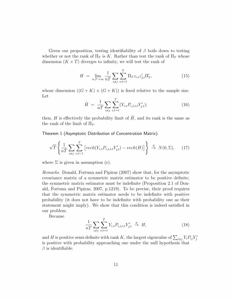
Given our proposition, testing identifiability of β boils down to testingwhether or not the rank of ΠT is K. Rather than test the rank of ΠT whosedimension (K × T ) diverges to infinity, we will test the rank of

H = limn,T→∞

1

nT

∑i 6=j

T∑s,t=1

ΠT zi,sz′j,tΠ

′T , (15)

whose dimension ((G+K) × (G+K)) is fixed relative to the sample size.Let

H =1

nT

∑i 6=j

T∑s,t=1

(Yi,sPi,j,s,tY′j,t); (16)

then, H is effectively the probability limit of H, and its rank is the same asthe rank of the limit of ΠT .

Theorem 1 (Asymptotic Distribution of Concentration Matrix).

√T

1

nT

∑i 6=j

T∑s,t=1

[vech(Yi,sPi,j,s,tY

′j,t)− vech(H)

] d→ N(0,Σ), (17)

where Σ is given in assumption (e).

Remarks. Donald, Fortuna and Pipiras (2007) show that, for the asymptoticcovariance matrix of a symmetric matrix estimator to be positive definite,the symmetric matrix estimator must be indefinite (Proposition 2.1 of Don-ald, Fortuna and Pipiras, 2007, p.1219). To be precise, their proof requiresthat the symmetric matrix estimator needs to be indefinite with positiveprobability (it does not have to be indefinite with probability one as theirstatement might imply). We show that this condition is indeed satisfied inour problem.

Because1

nT

∑i 6=j

T∑s,t=1

Yi,sPi,j,s,tY′j,t

p→ H, (18)

andH is positive semi-definite with rankK, the largest eigenvalue of∑

i 6=j YiPijY′j

is positive with probability approaching one under the null hypothesis thatβ is identifiable.

11

For (G+K)× 1 vector a,

a′1

nT

∑i 6=j

T∑s,t=1

Yi,sPi,j,s,tY′j,ta =

1

nT

∑i 6=j

T∑s,t=1

b′i,sbj,t

=1

nT

(n∑i=1

T∑s=1

b′i,s

n∑j=1

T∑t=1

bj,t −n∑i=1

b′ibi

)

=1

T

[(n− 1)b′b−

G+K∑k=1

V ar(bk)

](19)

where bi,t = (Z ′Z)−12 zi,tY

′i,ta, b = (1/n)

∑ni=1

∑Tt=1 bi,t, and V ar(bk) is the

sample variance of the k-th element of∑T

t=1 bi,t. For given n and T , the sum

of the variances of∑T

t=1 bi,t can be larger than nb′b with positive probability,provided that the support of vi is large enough, Thus, the smallest eigenvalueis negative with positive probability. Therefore, the necessary condition ofDonald et al. (2007) is satisfied provided that the support of vi is large enoughgiven Z.

Theorem 1 provides a basis for testing the rank of H. Therefore we willextend Donald et al.’s (2007) approach to symmetric matrices. FollowingKleibergen and Paap (2006) we may also normalize H and consider CHC ′

where C is a (G+K)× (G+K) non-singular matrix. For example, C maybe the square root of the covariance matrix of the endogenous variables.

Corollary 1 (Asymptotic Distribution of Scaled Concentration Matrix) In additionto Assumptions (a)–(e), suppose that

(f) D+G+K(C ⊗ C)D+

G+K has rank (G+K)(G+K + 1)/2.

Then √Tvech(CHC ′ − CHC ′) d→ N(0,Ω), (20)

where

Ω = D+G+K(C⊗C)D+

G+KΣD+′G+K(C ′⊗C ′)D+′

G+K , D+G+K = (D′G+KDG+K)−1D′G+K

and DG+K is the (G + K)2 × (G + K)(G + K + 1)/2 duplication matrix(Magnus and Neudecker, 1999, p.49).

Given the asymptotic normality of H, we employ Donald et al.’s (2007)

12

implementation of Kleibergen and Paap’s (2006) singular value decomposi-tion (SVD) rank test. For completeness, we provide the definition of the teststatistic.

To test that the instruments are orthogonal, we consider the null hy-pothesis that H is rank K against the alternative hypothesis that H is rank(K + 1). To test that the instruments are not relevant, we test the null hy-

pothesis that H is rank (K − 1) against the alternative hypothesis that His rank K. Let K0 be the rank under the null hypothesis. That is, K0 = Kunder the first null hypothesis and K0 = K − 1 under the second null hy-pothesis.

For the notational simplicity, we assume that H is used. Because H issymmetric, its singular value decomposition is identical to the Schur decom-position of H:

H = UDU ′ =

[U11 U12

U21 U22

] [D11 00 D22

] [U ′11 U ′21

U ′12 U ′22

], (21)

where U is a unitary matrix, D is a diagonal matrix whose diagonal ele-ments are the eigenvalues of H in non-increasing order, U11 and D11 are(K0 ×K0), U12 and U ′21 are (K0 × (K +G−K0)), and U22 and D22 are((K +G−K0)× (K +G−K0)). Define

A⊥ =

[U12

U22

]U22(U22U

′22)−

12

=

[U12

U22

], (22)

B⊥ = A′⊥, (23)

Λ = (U22U′22)−

12U22D22U

′22(U22U

′22)−

12 , (24)

Then under the null hypothesis that the rank of H is K0, it follows fromProposition 4.1 of Donald et al. (2007) that

T · vech(Λ)′Ω−1vech(Λ)d→ χ2

(K+G−K0)(K+G−K0+1)/2, (25)

where

Ω = D+K+G−K0

(B⊥ ⊗ A′⊥)DG+K−1ΣD′G+K−K0(B′⊥ ⊗ A⊥)D+′

K+G−K0,

13

D+K+G−K0

= (D′K+G−K0DK+G−K0)

−1D′K+G−K0and DK+G−K0 is the

((K +G−K0)2 × (K +G−K0)(K +G−K0 + 1)/2) duplication matrix.

We suggest the following testing procedure:

Step 1. Test if K0 = K. If this null is rejected, the model is misspecified. Ifthis null is not rejected, proceed to step 2.

Step 2. Test if K0 = K − 1. If this null hypothesis is rejected, the model iscorrectly specified and the parameter is identified (thus we fail to reject thenull hypothesis that the model is correct and the parameter is identified).If the second smallest eigenvalue is also zero, then the parameter is notidentified.

To make our testing procedure operational, one needs a consistent esti-mator of Σ, Σ. We need to find the asymptotic covariance matrix of the vechof

1

nT

∑i 6=j

T∑t=1

Yi,tPi,j,t,tY′j,t. (26)

For the factor model, we propose the following estimator of the asymptoticcovariance matrix:

Σ =1

n2T

T∑t=1

[∑i<j

vech(Yi,tYj,t + Yj,tY′i,t)vech(Yi,tYj,t + Yj,tY

′i,t)′

−µtµ′t] , (27)

where µt = (1/n)∑

i 6=j(vech(Yi,tYj,t + Yj,tYi,t)).

Proposition 2 (Consistency of the Asymptotic Covariance Matrix Estimator) Sup-pose that Assumptions (a)–(e) hold. Then

Σp→ Σ. (28)

4 Monte Carlo Experiments

We consider data generating processes (DGPs) calibrated on an asset pricingmodel with parameters estimated from U.S. data. We consider the traditional

14

CAPM model with parameters calibrated using gross returns on the three-month Treasury-bill and the 25 Fama and French size and book-to-marketportfolios from 1952:2 to 2000:4, for a total of 195 time series observations.The data are the same as in Gospodinov et al. (2013).

We consider three data generating processes (DGPs). In the first DGP,the parameter β is the following CAPM model is identified:

rigt = βft + σεigt, (29)

figt = ft + σηigt, (30)

ft = µf + σfζt, (31)

for i = 1, ..., n, g = 1, ..., G, t = 1, ..., T , where G ∈ 1, 5 is the number ofFama-French portfolios, n ∈ 100, 200 is the number of assets in each group,and T ∈ 100, 200 is the number of time periods. Because the identifiabilityof β does not depend on its value, the value of β is set to 1 without ofgenerality. The scalar common factor ft is the simulated market return attime t (generated from a normal with mean zero and variance σ2

f , where σ2f

is set to the variance of the market return in the data, σ2f = 0.0066).6 The

calibrated value of σ is based on Ang, Liu and Schwarz (2008): σ2 = 0.1225.εigt, ηigt and ζt are independent iid standard normal random variables.

To see why β is identifiable in this model rewrite the model using thenotation in the previous section as:

x = (`G ⊗ f)⊗ `Ngt + vx

= ZΠx + vx, (32)

y = (`G ⊗ f)⊗ `Ngtβ + ε

= ZΠxβ + vy, (33)

where Z = IGT ⊗ `Ngt , Πx = `G ⊗ f , Πy = Πxβ, vx = ση, vy = ε − vxβ.Then note that

Π = [Πx Πy] = [`G ⊗ f (`G ⊗ f)β] (34)

actually has rank 1 with probability one. Thus, β is identifiable with proba-bility one in this model.

6The mean of the market return for the sample period we consider is 0.0191 and it isindeed close to zero, so we set µf = 0.

15

We calculate the test statistic for testing that Π has rank 0 (under-identification) and the test statistic for testing that Π has rank 1 (correctspecification). Then we calculate frequencies in which each of the two nullhypotheses is rejected at the 5% significance level over 1,000 Monte Carlosimulations. Table 1 shows that the rank 0 test always rejects the null ofunder-identification while the rank 1 tends to have good size across differentsample sizes and portfolio sizes.

Next, we consider an alternative hypothesis under which the model ismisspecified. Specifically, we replace equation (29) by

rigt = ag + βft + σεigt, (35)

where ag is a portfolio-specific mean that is 0.025 times the sample means ofthe portfolio returns:

[1.0131 1.0394; 1.0394 1.0460 1.0492 1.0286 1.0369 1.0423 1.0441 1.0474]′.

The tests always have power one when the sample mean is used as ag. Tomake the Monte Carlo experiment more meaningful, we use 0.025 times thesample portfolio means. To see the effect of G, n and T on the power ofthe tests, we multiply the sample mean by 0.05. The portfolio specific meancould be interpreted as measurement error that does not disappear asymp-totically when constructing portfolio averages. Thus, this is a case in whichthe researcher has chosen a characteristic to sort portfolios that results inlarge measurement errors and renders the parameter estimate inconsistent.As a result the population first-stage regression coefficient matrix takes theform of

Π = [Πx Πy] = [`G ⊗ f (`G ⊗ f)β + a⊗ `T ] (36)

The rank of this matrix is 2 with probability one, meaning that the model ismisspecified.

Table 2 shows the empirical rejection frequencies when testing the nullhypothesis that Π has rank 0 and when testing the null hypothesis thatΠ has rank 1. Again the rank 0 test always rejects the null hypothesis ofunder-identification. The rank 1 test rejects the null hypothesis of correctspecification with probability much higher than the nominal size. The rejec-tion frequency of the rank 1 test is increasing in sample sizes and approachesone as expected.

16

Finally, we consider a DGP in which there is no factor structure:

rigt = σεigt,

figt = σηigt,

Using the notation in the previous section, the model can be written as

x = ZΠx + vx,

y = xβ + ε = ZΠxβ︸︷︷︸=Πy

+ vy,

where Πx = 0. Because rank(ΠT ) =rank

([00

])= 0, the parameter β is

not identified. Because the rank 0 test is designed to test the null of under-identification, not rejecting this null means that the parameter is likely tobe under-identified. Table 3 shows that the rank 0 test is undersized andsuggests that one would conclude that the parameter is not identified. It isinteresting to note that the rejection frequencies of the rank 1 test are verysmall in this case. This is because the rank 1 test is designed to test the nullhypothesis that the rank is one against the alternative hypothesis that therank is higher than one.

5 Conclusion

This paper proposed a new test to evaluate the portfolio choice in widely-used finance regressions based on portfolio returns. The new test allowsresearchers to tackle the empirical problem that empirical results are sensitiveto the portfolio choice. This paper provides techniques to evaluate whetherthe portfolio choice is appropriate by testing the validity of the choice of howto group assets into portfolios and the exogeneity of the portfolio choice. Onlyunder these condition the parameters of interest(such as β and the price ofrisk of a portfolio) can be correctly estimated. Monte Carlo simulations basedon the CAPM model demonstrate the good size and power properties of ourtest.

While we motivate this problem from the portfolio choice perspective,our test can be used to test for identification in group and pseudo and paneldata models as well.

17

Appendix

First, we present a lemma that is an extension of Lemma A2 of Chao et al.(2012) to our dependence structure of the error terms.

Lemma. Suppose that Assumptions (a)-(e) hold. Then

Sn,T =1√nT

∑i 6=j

T∑s,t=1

vech(ΠT zi,sPi,j,s,tvj,t + vi,sPi,j,s,tz′j,tΠ

′T + vi,sPi,j,s,tv

′j,t)

d→ N(0,Σ). (37)

Proof of Lemma. For notational simplicity, and suppose that ft and vi,t arescalar and that we focus on the (1, 1) element of Sn,T . The desired resultfollows from applying the Cramer-Wold device to this scalar result.

Because P = IT ⊗ (1/n)`n`′n is block diagonal and the (1, 1) element of

ΠT zi,s is fs, we can write the (1,1) element of Sn,T as

Sn,T =1

n√nT

∑i 6=j

T∑t=1

(ftvi,t + ftvj,t + vi,tvj,t), (38)

with some notational abuse. Let

st =1

n√nT

∑i 6=j

(ftvi,t + ftvj,t + vi,tvj,t). (39)

Then we can rewrite Sn,T as

Sn,T =T∑t=1

st. (40)

Let Ft denote the sigma field generated by fs+1, v1,s, v2,s, . . . , vn,sts=1.Because vi,s and vj,t are independent for all i, j, s, t such that i 6= j or s 6= t,st is a martingale difference sequence relative to Ft. If we show

T∑t=1

E[s2t |Ft−1, Z

]→ Σ a.s., (41)

T∑t=1

E[s2t I(|st| ≥ ε)|Z] → 0 a.s., (42)

18

for each ε > 0, the martingale central limit theorem (Theorem 35.12 ofBillinsgley, 1995, p.476) gives

P (Sn,T ≤ x|Z) → 1√Σ

Φ

(x√Σ

)a.s. (43)

for all x ∈ < conditional on Z. Note that, for ε > 0 :

supn,T

E[P (Sn,T ≤ x|Z)1+ε] <∞ (44)

because probabilities are bounded between zero and one. Given that (44)holds, it follows from the dominated convergence theorem (Corollary inBillingsley, 1995, p.338) and (43) that7

P (Sn,T ≤ x) → 1√Σ

Φ

(x√Σ

), (45)

completing the proof for the case in which vi,t is scalar.

It remains to show (41) and (42). Note that

E(s2t |Z)

=1

n3T

∑i 6=j

∑k 6=`

[E(f 2t vi,tvk,t|Z) + E(f 2

t vi,tv`,t|Z) + E(f 2t vj,tvk,t|Z) + E(f 2

t vj,tv`,t|Z)

+E(vi,tvj,tvk,tv`,t|Z) + 2E(f 2t vi,tvj,t) + 2E(ftv

2i,tvj,t|Z) + 2E(ftvi,tv

2j,t|Z)]

=4(n− 1)2

n3T

n∑i=1

E(f 2t v

2i,t|Z) +

1

n3T

∑i 6=j

∑k 6=`

E(vi,tvj,tvk,tv`,t|Z)]. (46)

The first term on the right hand side of (46) can be written as

4(n− 1)2

n3T

n∑i=1

E(f 2t v

2i,t|Z) =

4(n− 1)2

n3Tσ2f

n∑i=1

σ2i,t. (47)

The summation over i 6= j and k 6= ` in the second term on the right hand

7Note that the unconditional probability is the expected value of the conditional prob-ability.

19

side of (46) can be split into summations over three sets of i, j, k, `:

I0 = (i, j, k, `) : i, j, k, ` are distint from each other, (48)

I1 = (i, j, k, `) : only one pair are identical among i 6= j, k 6= `,

i.e., (i = k and j 6= `) or (i 6= k and j = `) or (i = ` and j 6= k) or (i 6= ` and j = k),(49)

I2 = (i, j, k, `) : two pairs are identical among i 6= j, k 6= `,

i.e., (i = k and j = `) or (i = ` and j = k). (50)

The expectations in the second term on the right hand side of (46) are zerowhen i, j, k, ` are in I0 and I1 and thus can be written as

1

n3T

∑i 6=j

∑k 6=`

E(vi,tvj,tvk,tv`,t|Z) =1

n3T

∑i,j,k,`∈I2

E(vi,tvj,tvk,tv`,t|Z)

=2

n3T

∑i 6=j

σ2i,tσ

2j,t (51)

where σ2i,t = E(v2

i,t|Z). Because st is a martingale difference sequence relativeto Ft conditional on Z, it follows from (46), (47), (51) and Assumption (e)that

T∑t=1

E(s2t |Ft, Z

)=

4σ2f (n− 1)2

n3T

T∑t=1

n∑i=1

σ2i,t +

2

n3T

∑i 6=j

T∑t=1

σ2i,tσ

2j,t

=4σ2

f

nT

T∑t=1

n∑i=1

σ2i,t +O(n−1)

→ Σ a.s. (52)

Thus the law of iterated expectations completes the proof of (41).

20

To prove (42), write∑T

t=1E(s4t |Z) as

T∑t=1

E(s4t |Z) =

1

n2T 2

n∑j1,j2,j3,j4=1

E(f 4t vj1vj2vj3vj4)

+4

n3T 2

∑j1,j2,j3,j4,j5,j4 6=j5

E(f 3t vj1vj2vj3vj4vj5)

+6

n4T 2

∑j1,j2,j3,j4,j5,j6,j3 6=j4,j5 6=j6

E(f 2t vj1vj2vj3vj4vj5vj6)

+4

n5T 2

∑j1,j2,j3,j4,j5,j6,j7,j2 6=j3,j4 6=j5,j6 6=j7

E(ftvj1vj2vj3vj4vj5vj6vj7)

+4

n6T 2

∑j1 6=j2,j3 6=j4,j5 6=j6,j7 6=j8

E(vj1vj2vj3vj4vj5vj6vj7vj8)

= E1 + E2 + E3 + E4 + E5. (53)

It follows from the assumption of mutual independence that

E1 = O( n

n2T 2

)+O

(n2

n2T 2

), (54)

E2 = O

(n2

n3T 2

), (55)

E3 = O

(n2

n4T 2

)+O

(n3

n4T 2

), (56)

E4 = O

(n2

n5T 2

)+O

(n3

n5T 2

), (57)

E5 = O

(n2

n6T 2

)+O

(n3

n6T 2

)+O

(n4

n6T 2

), (58)

almost surely. Thus,T∑t=1

E(s4t |Z) = O(T−1) (59)

almost surely from which (42) follows.

Proof of Proposition 1. Suppose that the rank of ΠT is K. Pre-multiplyingeach side of the reduced-form equation (13) by G× (G+K) matrix c[−β′ IG]

21

yieldsc(yi,t − β′xi,t) = c[1 − β′]ΠT zi,t + c[−β′ IG]vj, (60)

which implies that c[−β′ IG]ΠT = 0 must hold. Because ΠT has rank K,c[1 − β′] is identified up to scale. Setting c = 1, β is identified.

Suppose that the model is correctly specified and that the parameter βis identified. Then the former implies Πy,T = β′Πx,T while the latter impliesthat the rank of Πx,T is K. Therefore the rank of ΠT is K.

Proof of Theorem 1. Because

1√nT

∑i 6=j

T∑s,t=1

Yi,sPi,j,s,tY′j,t =

1

n√nT

∑i 6=j

T∑t=1

ΠT zi,tz′j,tΠ

′T +

1

n√nT

∑i 6=j

T∑t=1

ΠT zi,tv′j,t

+1

n√nT

∑i 6=j

T∑t=1

vi,tz′j,tΠ

′T +

1

n√nT

∑i 6=j

T∑t=1

vi,tv′j,t,(61)

we have

1√nT

∑i 6=j

T∑s,t=1

Yi,sPi,j,s,tY′j,t −

1

n√nT

∑i 6=j

T∑t=1

ΠT zi,tz′j,tΠ

′T

=1

n√nT

∑i 6=j

T∑t=1

ΠT zi,tv′j,t +

1

n√nT

∑i 6=j

T∑t=1

vi,tz′j,tΠ

′T +

1

n√nT

∑i 6=j

T∑t=1

vi,tv′j,t

=1

n√nT

∑i 6=j

T∑t=1

ftv′j,t +

1

n√nT

∑i 6=j

T∑t=1

vi,tf′t +

1

n√nT

∑i 6=j

T∑t=1

vi,tv′j,t

=1√nT

T∑t=1

ft

n∑j=1

v′j,t +1√nT

T∑t=1

n∑i=1

vi,tf′t +

1

n√nT

∑i 6=j

T∑t=1

vi,tv′j,t

= I + II + III. (62)

The variance-covariance matrix of I is

1

nT

T∑s,t=1

n∑i,j=1

E[vech(fsv′i,s)vech(ftv

′j,t)′] =

1

nT

T∑t=1

n∑i=1

E[vech(ftv′i,t)vech(ftv

′i,t)′].

(63)

22

Similarly, the covariance matrix between I and II and the variance covariancematrix of II are given by

1

nT

T∑t=1

n∑i=1

E[vech(ftv′i,t)vech(vi,tf

′t)′], (64)

1

nT

T∑t=1

n∑j=1

E[vech(vj,tf′t)vech(vj,tf

′t)′], (65)

respectively. I and III are uncorrelated because

1

nT

T∑s,t=1

n∑i=1

∑j 6=k

E[vech(fsv′i,s)vech(vj,tv

′k,t)′] =

1

nT

T∑t=1

∑j 6=k

E[vech(ftv′j,t)vech(vj,tv

′k,t)′]

+1

nT

T∑t=1

∑j 6=k

E[vech(ftv′k,t)vech(vj,tv

′k,t)′]

= 0 (66)

Analogously, II and III are uncorrelated. III is Op(n−1). Therefore it

follows from our lemma that

vech(I + II + III)d→ N(0,Σ). (67)

Thus, it follows from (62)—(67) that

1√NT

∑i 6=j

vech(viPijv′j)

d→ N(0,Σ). (68)

Proof of Corollary 1. The corollary follows from Theorem 1 because

vech(CHC ′) = D+n vec(CHC

′) = D+n vec(CHC

′)

= D+n (C ⊗ C)vec(H) = D+

n (C × C)D+n vech(H). (69)

Proof of Proposition 2.

To simplify the notation, we assume that ft and vi,t scalar. Because Pi,j,t,t =

23

1/n, Σ can be written as

Σ =2

n2T

T∑t=1

∑i 6=j

(ft + vi,t)2(ft + vj,t)

2 −

(1

n

∑i 6=j

(ft + vi,t)(ft + vj,t)

)2 .(70)

Repeating the martingale argument in the proof of the lemma, it can beshown that

Σ =2

n2T

T∑t=1

∑i 6=j

f 2t (v2

i,t + v2j,t) + op(1)

=2(n− 1)

n2T

T∑t=1

n∑i=1

f 2t v

2i,t +

2(n− 1)

n2T

T∑t=1

n∑j=1

f 2t v

2j,t + op(1)

= 2σ2f

1

n

n∑i=1

σ2i,t + 2σ2

f

1

n

n∑j=1

σ2j,t + op(1)

= 4σ2f

1

n

n∑i=1

σ2i,t + op(1). (71)

Thus, Σ is consistent for Σ.

24

References

1. Anatolyev, Stanislav, and Nikolay Gospodinov (2011), “Specification Test-

ing in Models with Many Instruments,” Econometric Theory, 27, 427–441.

2. Ang, Andrew, Jun Liu, and Krista Schwarz (2009), “Using Individual Stocks

or Portfolios in Tests of Factor Models”, SSRN Working Paper,

http://ssrn.com/abstract=1106463.

3. Angrist, Joshua D. (1988), “Grouped Data Estimation and Testing in Simple

Labor Supply Models,” Journal of Econometrics, 47, 243–266.

4. Bekker, Paul A. (1994), “Alternative Approximations to the Distributions

of Instrumental Variables Estimators,” Econometrica, 62, 657–681.

5. Billingsley, Patrick (1995), Probability and Measures, Third Edition, John

Wiley & Sons: New York, NY.

6. Chao, John C., Norman R. Swanson, Jerry A. Hausman, Whitney K. Newey

and Tiemen Woutersen (2012), “Asymptotic Distribution of JIVE in a Het-

eroskedastic IV Regression with Many Instruments,” Econometric Theory,

28, 42–86.

7. Chao, John C., Jerry A. Hausman, Whitney K. Newey, Norman R. Swanson

and Tiemen Woutersen (2014), “Testing Overidentifying Restrictions with

Many Instruments and Heteroskedasticity,” Journal of Econometrics, 178,

15–21.

8. Cochrane, John H. (2005), Asset Pricing, Princeton University Press.

9. Deaton, Angus (1985), “Panel Data from a Time Series of Cross-Sections,”

Journal of Econometrics, 30, 109–126.

10. Donald, Stephen G., Natercia Fortuna and Vladas Pipiras (2007), “On Rank

Estimation in Symmetric Matrices: The Case of Indefinite Matrix Estima-

tors,” Econometric Theory, 23, 1217–1232.

11. Fama, Eugene F. and Kenneth R. French (1992), “The Cross-Section of

Expected Stock Returns,” Journal of Finance 47:2, 427–65.

25

12. Fama, Eugene F. and Kenneth R. French (2004), “The Capital Asset Pricing

Model: Theory and Evidence”, Journal of Economic Perspectives 18(3), 25–

46.

13. Gospodinov, Nikolay, Raymond Kan and Cesare Robotti (2013), “Chi-squared

Tests for Evaluation and Comparison of Asset Pricing Models”, Journal of

Econometrics 173, 108–125.

14. Kandel, S. and R.F. Stambaugh (1995), “Portfolio Inefficiency and the Cross-

Section of Expected Returns,” Journal of Finance 50, 157-184.

15. Kleibergen, Frank, and Richard Paap, (2006), “Generalized Reduced Rank

Tests Using the Singular Value Decomposition,” Journal of Econometrics,

133, 97–126.

16. Kleibergen, Frank, and Zhaoguo Zhan (2013), “Unexplained Factors and

Their Effects on Second Pass R-squared’s and t-tests”, mimeo, Brown and

Tsinghua University.

17. Koopmans, Tjalling C., and William C. Hood, (1953), “The Estimation

of Simultaneous Linear Economic Relationships,” in W.C. Hood and T.C.

Koopmans, eds., Studies in Econometric Methods, Yale University Press:

New Haven, CT, Chapter 6.

18. Kunitomo, Naoto (1980), “Asymptotic Expansions of Distributions of Esti-

mators in a Linear Functional Relationship and Simultaneous Equations,”

Journal of the American Statistical Associations, 75, 693–700.

19. Lettau, Martin, and Sydney Ludvigson (2001), “Consumption, Aggregate

Wealth and Expected Stock Returns,” Journal of Finance 56, 815–849.

20. Magnus, Jan R., and Heinz Neudecker (1999), Matrix Differential Calculus

with Applications in Statistics and Econometrics, Revised Edition, John

Wiley & Sons: Chichester, England.

21. Morimune, Kimio (1983), “Approximate Distributions of the k-class Esti-

mators When the Degree of Overidentifiability is Large Compared with the

Sample Size,” Econometrica, 51, 821–841.

22. Verdelhan, Adrien (2012), “The Share of Systematic Variation in Bilateral

Exchange Rates”, SSRN Working Paper, http://ssrn.com/abstract=1930516.

26

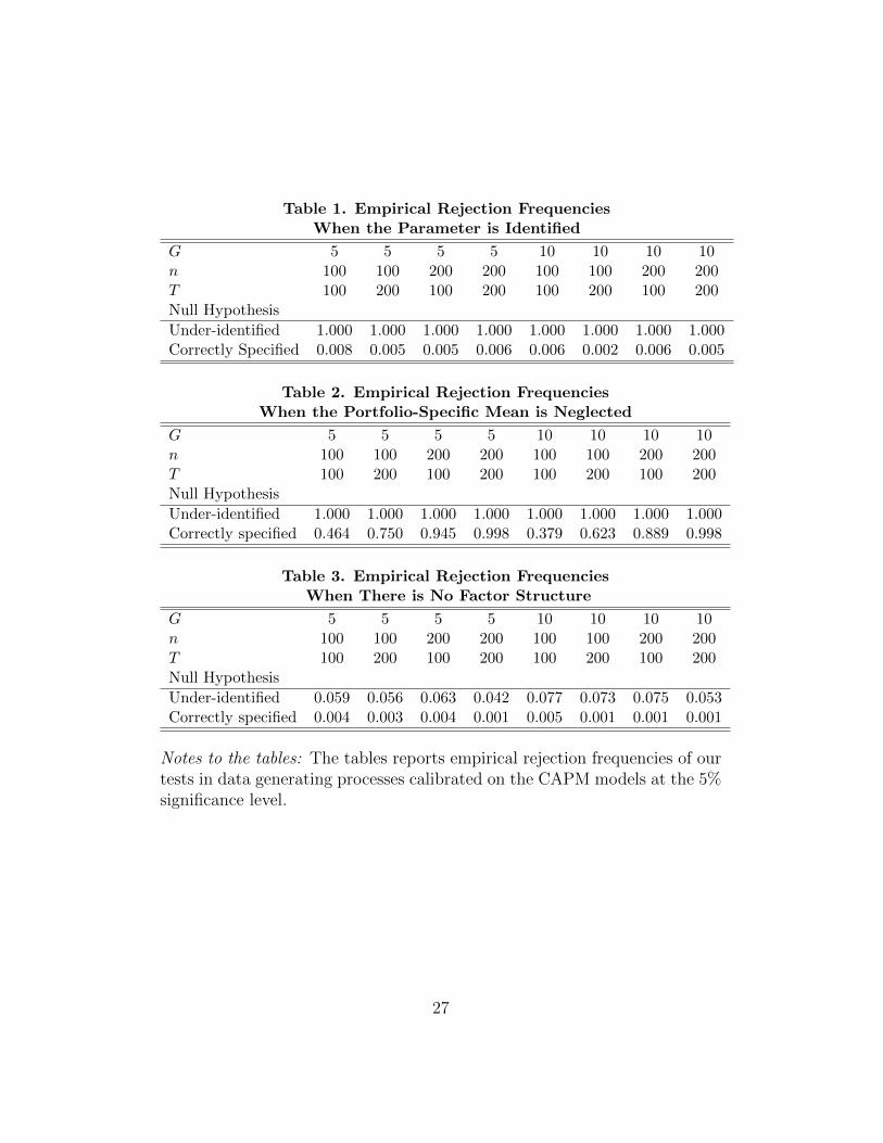
Table 1. Empirical Rejection FrequenciesWhen the Parameter is Identified

G 5 5 5 5 10 10 10 10n 100 100 200 200 100 100 200 200T 100 200 100 200 100 200 100 200Null Hypothesis

Under-identified 1.000 1.000 1.000 1.000 1.000 1.000 1.000 1.000Correctly Specified 0.008 0.005 0.005 0.006 0.006 0.002 0.006 0.005

Table 2. Empirical Rejection FrequenciesWhen the Portfolio-Specific Mean is Neglected

G 5 5 5 5 10 10 10 10n 100 100 200 200 100 100 200 200T 100 200 100 200 100 200 100 200Null Hypothesis

Under-identified 1.000 1.000 1.000 1.000 1.000 1.000 1.000 1.000Correctly specified 0.464 0.750 0.945 0.998 0.379 0.623 0.889 0.998

Table 3. Empirical Rejection FrequenciesWhen There is No Factor Structure

G 5 5 5 5 10 10 10 10n 100 100 200 200 100 100 200 200T 100 200 100 200 100 200 100 200Null Hypothesis

Under-identified 0.059 0.056 0.063 0.042 0.077 0.073 0.075 0.053Correctly specified 0.004 0.003 0.004 0.001 0.005 0.001 0.001 0.001

Notes to the tables: The tables reports empirical rejection frequencies of ourtests in data generating processes calibrated on the CAPM models at the 5%significance level.

27