Geophys. J. Int. (2006) 167, 635–648 doi: 10.1111/j.1365-246X.2006.03133.x GJI Geomagnetism, rock magnetism and palaeomagnetism Testing statistical palaeomagnetic field models against directional data affected by measurement errors A. Khokhlov, 1,2 G. Hulot 2 and C. Bouligand 2 1 International Institute of Earthquake Prediction Theory and Mathematical Geophysics 79, b2, Warshavskoe shosse 117556 Moscow, Russia 2 Equipe de G´ eomagn´ etisme, Institut de Physique du Globe de Paris (Institut de recherche associ´ e au CNRS et ` a l’Universit´ e Paris 7), 4, Place Jussieu, 75252, Paris, France. E-mail: [email protected] Accepted 2006 July 7. Received 2006 June 22; in original form 2005 December 30 SUMMARY In a previous paper, Khokhlov et al. introduced a method to test the compatibility of so-called ‘giant Gaussian process’ (GGP) statistical models of the palaeomagnetic field against any palaeosecular variation database. This method did not take measurement errors into account. It therefore lacked practical usefulness. In the present paper, we remedy this and generalize the method to account for measurement errors in a way consistent with both the assumptions underlying the GGP approach and the nature of those errors. The method is implemented to test GGP models against any directional data set affected by Fisherian errors. Simulations show that the method can usefully discriminate which GGP model best explains a given data set. Applying the method to test six published GGP models against a test Bruhnes stable polarity data set extracted from the Quidelleur et al. database, it is found that all but one model (that of Quidelleur & Courtillot) should be rejected. Although this result should be taken with care, and does not necessarily imply that this model is superior to other models (Quidelleur & Courtillot precisely used the Quidelleur et al. database to infer their model), it clearly shows that in practice also, and with the databases currently available, the method can discriminate various candidate GGP models. It also shows that the statistical behaviour of the geomagnetic field at times of stable polarity can indeed be described in a consistent way in terms of a GGP model. This ‘forward’ testing method could ultimately be used to design an ‘inverse’ approach to GGP modelling of the palaeomagnetic field. Key words: archaeomagnetism, geomagnetism, palaeomagnetism, potential field, spherical harmonics, statistical methods. INTRODUCTION Thanks to the large amount of magnetic data provided by satel- lite missions spherical harmonic models of the main magnetic field produced within the core can readily be computed, providing high- resolution pictures of the way this field has been behaving over the past few decades (Hulot et al. 2002). Additional information can also be recovered from observations carried out by many genera- tions of observers, explorers and navigators worldwide to produce spherical harmonic models describing the main magnetic field over the past four centuries (Jackson et al. 2000). Reconstructing similar, albeit much less accurate, spherical harmonic models of the Earth’s main magnetic field further back in time is also possible (Hongre et al. 1998; Korte & Constable 2005). This, however, requires that indirect measurements be used, only available through human arte- facts, lava flows and sediments that have been magnetized in the ancient field. It also requires that a good age control of each sample is available to ensure a satisfying synchronization of the data used in computing spherical harmonic models for a given epoch. Because changes in the non-dipole component of the main field occur on short timescales for small spatial scales (Hulot & Le Mou¨ el 1994), a poor control indeed limits our ability to produce such spherical harmonic models back in time (so far, only up to 7000 yr in the past, Korte & Constable 2005). To recover information about the Earth’s main magnetic field further back in time, one must rely on palaeomagnetic data and acknowledge the impossibility of accurately (within a few decades at most) synchronizing data acquired at different loca- tions. This is especially true for the so-called palaeosecular variation (Quidelleur et al. 1994; Johnson & Constable 1996; McElhinny & McFadden 1997) and palaeointensity (Tanaka et al. 1995; Perrin & Schnepp 2004) databases covering the past few million years. Those databases encompass data recovered from volcanic samples and tes- tifying for the instantaneous value of the direction and/or intensity of the field at well-known locations but poorly known times (typically within much more than a millennium). Fortunately, ages can nev- ertheless be measured with enough accuracy to identify the chron during which each of these samples acquired its magnetization. As- suming that the geodynamo essentially remained in a stationary state at times of stable polarity, this then opens the possibility, recognized C 2006 The Authors 635 Journal compilation C 2006 RAS Downloaded from https://academic.oup.com/gji/article/167/2/635/562682 by guest on 14 April 2022

Welcome message from author
This document is posted to help you gain knowledge. Please leave a comment to let me know what you think about it! Share it to your friends and learn new things together.
Transcript
Geophys. J. Int. (2006) 167, 635–648 doi: 10.1111/j.1365-246X.2006.03133.x
GJI
Geo
mag
netism
,ro
ckm
agne
tism
and
pala
eom
agne
tism
Testing statistical palaeomagnetic field models against directionaldata affected by measurement errors
A. Khokhlov,1,2 G. Hulot2 and C. Bouligand2
1International Institute of Earthquake Prediction Theory and Mathematical Geophysics 79, b2, Warshavskoe shosse 117556 Moscow, Russia2Equipe de Geomagnetisme, Institut de Physique du Globe de Paris (Institut de recherche associe au CNRS et a l’Universite Paris 7), 4, Place Jussieu, 75252,
Paris, France. E-mail: [email protected]
Accepted 2006 July 7. Received 2006 June 22; in original form 2005 December 30
S U M M A R YIn a previous paper, Khokhlov et al. introduced a method to test the compatibility of so-called‘giant Gaussian process’ (GGP) statistical models of the palaeomagnetic field against anypalaeosecular variation database. This method did not take measurement errors into account.It therefore lacked practical usefulness. In the present paper, we remedy this and generalizethe method to account for measurement errors in a way consistent with both the assumptionsunderlying the GGP approach and the nature of those errors. The method is implemented to testGGP models against any directional data set affected by Fisherian errors. Simulations showthat the method can usefully discriminate which GGP model best explains a given data set.Applying the method to test six published GGP models against a test Bruhnes stable polaritydata set extracted from the Quidelleur et al. database, it is found that all but one model (that ofQuidelleur & Courtillot) should be rejected. Although this result should be taken with care, anddoes not necessarily imply that this model is superior to other models (Quidelleur & Courtillotprecisely used the Quidelleur et al. database to infer their model), it clearly shows that inpractice also, and with the databases currently available, the method can discriminate variouscandidate GGP models. It also shows that the statistical behaviour of the geomagnetic field attimes of stable polarity can indeed be described in a consistent way in terms of a GGP model.This ‘forward’ testing method could ultimately be used to design an ‘inverse’ approach to GGPmodelling of the palaeomagnetic field.
Key words: archaeomagnetism, geomagnetism, palaeomagnetism, potential field, sphericalharmonics, statistical methods.
I N T RO D U C T I O N
Thanks to the large amount of magnetic data provided by satel-
lite missions spherical harmonic models of the main magnetic field
produced within the core can readily be computed, providing high-
resolution pictures of the way this field has been behaving over the
past few decades (Hulot et al. 2002). Additional information can
also be recovered from observations carried out by many genera-
tions of observers, explorers and navigators worldwide to produce
spherical harmonic models describing the main magnetic field over
the past four centuries (Jackson et al. 2000). Reconstructing similar,
albeit much less accurate, spherical harmonic models of the Earth’s
main magnetic field further back in time is also possible (Hongre
et al. 1998; Korte & Constable 2005). This, however, requires that
indirect measurements be used, only available through human arte-
facts, lava flows and sediments that have been magnetized in the
ancient field. It also requires that a good age control of each sample
is available to ensure a satisfying synchronization of the data used in
computing spherical harmonic models for a given epoch. Because
changes in the non-dipole component of the main field occur on
short timescales for small spatial scales (Hulot & Le Mouel 1994),
a poor control indeed limits our ability to produce such spherical
harmonic models back in time (so far, only up to 7000 yr in the past,
Korte & Constable 2005).
To recover information about the Earth’s main magnetic field
further back in time, one must rely on palaeomagnetic data
and acknowledge the impossibility of accurately (within a few
decades at most) synchronizing data acquired at different loca-
tions. This is especially true for the so-called palaeosecular variation
(Quidelleur et al. 1994; Johnson & Constable 1996; McElhinny &
McFadden 1997) and palaeointensity (Tanaka et al. 1995; Perrin &
Schnepp 2004) databases covering the past few million years. Those
databases encompass data recovered from volcanic samples and tes-
tifying for the instantaneous value of the direction and/or intensity of
the field at well-known locations but poorly known times (typically
within much more than a millennium). Fortunately, ages can nev-
ertheless be measured with enough accuracy to identify the chron
during which each of these samples acquired its magnetization. As-
suming that the geodynamo essentially remained in a stationary state
at times of stable polarity, this then opens the possibility, recognized
C© 2006 The Authors 635Journal compilation C© 2006 RAS
Dow
nloaded from https://academ
ic.oup.com/gji/article/167/2/635/562682 by guest on 14 April 2022
636 A. Khokhlov, G. Hulot and C. Bouligand
long ago (see e.g. Merrill et al. 1996, for an extensive review of ear-
lier work), that at least some statistical properties could be recovered,
characterizing the ancient field at times of stable polarity over the
past millions years.
Several approaches have been used to try and infer such statis-
tical properties (again, see e.g. Merrill et al. 1996). One approach
has drawn particular attention, the so-called giant Gaussian process
(GGP) approach first introduced by Constable & Parker (1988), and
next generalized by Hulot & Le Mouel (1994) and Kono & Tanaka
(1995). In its most general form (see e.g. Hulot & Bouligand 2005),
this approach consists in
(1) using the classical spherical harmonic decomposition of the
Main Field:
B(�, �, �, t) = −∇[
a∞∑
l=1
l∑m=0(
a
�)l+1(
gml (t)cos m� + hm
l (t)sin m�)Pm
l (cos �)
], (1)
where gml (t) and hm
l (t) are the time-varying Gauss coefficients, adenotes the Earth’s radius and {�, �, �} are the standard spherical
coordinates (i.e. distance from the Earth’s centre, colatitude and
longitude), and
(2) assuming that the gml (t) and hm
l (t) are the coordinates of a
vector k(t) in a multidimensional model space, which behaves as a
single realization of a multidimensional stationary random Gaussian
process characterized by a statistical mean (or mean model) E(k(t))and a covariance matrix Cov(k(t), k(t ′)) (which may very well be
non-diagonal).
In addition to being defined with the help of a fully consistent for-
malism, this GGP approach has the unique advantage of providing
a common tool to analyse just as well the historical (Constable &
Parker 1988; Hulot & Le Mouel 1994), archaeomagnetic (Hongre
et al. 1998) and palaeomagnetic fields (Constable & Parker 1988
and many studies since, see e.g. Kono et al. 2000a; Tauxe & Kent
2004). Even more, it can also be used to carry on similar analysis
of the field produced by dynamo numerical simulations (Kono et al.2000b; McMillan et al. 2001; Bouligand et al. 2005). In the latter
case, considerable advantage can be taken of the fact that the Gauss
coefficients (and very long time-series) are readily available and
can thus be analysed in much detail without having to worry about
any observational errors. Those studies have shown that under rea-
sonable circumstances, the field produced by a numerical dynamo
is indeed compatible with a GGP description, which can then be
used to detect very interesting statistical properties, most notably,
spontaneous and forced (because of the boundary conditions im-
posed at the core–mantle boundary) symmetry breaking properties
(Bouligand et al. 2005; Hulot & Bouligand 2005). The GGP ap-
proach thus appears to potentially be a tool of choice to characterize
the Earth’s main magnetic field at various epochs (present and past),
detect possible changes in the regime of the geodynamo, some of
which could be due to changes in the boundary conditions, and de-
cide whether a numerical dynamo simulation is ‘Earth-like’ or not.
For this to be possible, we, however, need to have robust and sen-
sitive numerical tools to actually decide which GGP model best fits a
given data set. The issue is unfortunately not so trivial when the data
to be analysed are the palaeomagnetic data from the palaeosecular
variation databases (the largest available palaeomagnetic database
for that type of study). In that case indeed, because the (directional)
data are non-linearly related to the Gauss coefficients of the main
field, no simple method is available to directly produce estimates
of the mean and covariance matrix of the GGP process best de-
scribing the data. Furthermore, using approximate approaches can
easily lead to biased estimates (Khokhlov et al. 2001; Hatakeyama
& Kono 2001). The purpose of the present paper, which expends
on the earlier work of Khokhlov et al. (2001) (hereafter paper I), is
to show that in fact a rigorous method can be implemented which
(1) is fully consistent with all the assumptions involved in the GGP
approach, (2) takes into account the measurement errors provided
with each data point (a major improvement with respect to paper I),
(3) provides a rigorous quantified assessment of the compatibility
of any GGP model with any directional data set and (4) proves very
discriminating.
D E A L I N G W I T H E R RO R - F R E E
PA L A E O D I R E C T I O N A L DATA
In this section, we first recall the approach proposed in paper I to
test any error-free palaeodirectional data set. [Note, however, that
we will make use of slightly different notations to avoid confusion
among the various quantities we need to define. As a general rule,
in the present paper, we will indeed always make use of gothic
letters, namely g, s, k and p (possibly with indexes) for the various
probability density functions (PDFs) we will need to introduce.]
When dealing with such data, which consist in instantaneous
values of the palaeodirection recorded at times separated by much
more than the memory of the GGP process, each palaeomagnetic
datum can be viewed as a local (both in time and space) inde-
pendent realization of the GGP process. As a result, the covari-
ance matrix of the process can be assumed to be of the simplified
form Cov(k(t), k(t ′)) = Cov(k, k)δ(t − t ′) and temporal correla-
tions ignored altogether. Rewriting eq. (1) in the simplified form
B(�, �, �, t) = A(�, �, �)k(t), where A(�, �, �) is a ma-
trix projecting the multidimensional vector k(t) into the 3-D vec-
tor B(�, �, �, t), a given instantaneous value B of the field at a
given location (�, �, �) at the Earth’s surface can then itself be
viewed as a random drawing from a 3-D Gaussian distribution of
random vectors V characterized by E(V) = A(�, �, �)E(k) and
Cov(V, V) = A(�, �, �)Cov(k, k)A(�, �, �)T . Denote g, the
corresponding PDF in R3.
Next, introduce the spherical coordinates (u, ρ) of the vector
V (where u = V/|V | ∈ �, the unit sphere in R3, and ρ = |V |denotes the distance from the origin O of the sphere �). Denote s
the PDF associated with the direction u on �. This so-called angular
Gaussian distribution (Bingham 1983, in paper I, we also referred
to it as the Gaussian Directional distribution) is then defined by:
s(u) =∫ ∞
0
g(ρu) dρ. (2)
In a local Cartesian coordinate system, we may write E(V) = m =(m 1, m 2, m 3) and Cov(V , V) = [cov(Vi , V j )]. Then, let Λ = [�i j ]
be the inverse (hence, also symmetric) matrix of Cov(V , V). With
respect to these local Cartesian coordinates, the PDF of V is:
g(x1, x2, x3) =√
det Λ(2π )3
exp
[−1
2
3∑i, j=1
�i j (xi − mi )(x j − m j )
],
(3)
or
g(x) =√
det Λ(2π )3
exp
[−1
2(�(x − m), x − m)
]. (4)
Making use of the Λ-inner product (x, y)Λ = (Λx, y) =∑3i, j=1 �i j xi y j together with the corresponding Λ-norm |x|Λ =
C© 2006 The Authors, GJI, 167, 635–648
Journal compilation C© 2006 RAS
Dow
nloaded from https://academ
ic.oup.com/gji/article/167/2/635/562682 by guest on 14 April 2022
Testing statistical palaeomagnetic field models 637√(x, x)Λ, and turning back to the spherical coordinates (u, ρ) in R3,
we may then write:
g(ρu) =√
det Λ(2π )3
e− 12 |ρu−m|2Λρ2, (5)
and, after ρ-integration (eq. 2), finally get
s(u) = e− 1
2 m2
·√
det Λ4π |u|3Λ
[z
√2
π+ e
12 z2
(1 + z2)
[1 + Erf
(z√2
)]],
(6)
where
z = (m, u)Λ|u|Λ , m = |m|Λ, (7)
correspond to respectively the Λ-projection of m on the direction
u, and the Λ-norm of m. Since Λ is positive −m ≤ z ≤ m.
Eq. (6) makes it possible to predict the PDF of the direction of the
field at any location at the Earth’s surface. Any given GGP model
can then easily be tested against the data set corresponding to such
a location.
Unfortunately, relatively few data are usually available at a given
location. In paper I, we explained how this drawback could be over-
come, and sparse data distributed over various sites combined into
a uniformized data set to globally test the GGP model.
This consists in converting the directional data set {ui} under
consideration (where the ‘i’ index varies between 1 and N , the total
amount of data) into a univariate data set {t i} with the help of:
ti = P{u|si (u) ≥ si (ui )} =∫
{u|si (u)≥si (ui )}
si (u) dU, (8)
where dU is the elementary surface about u on �, and testing the
distribution of the {t i} against a uniform probability density over
the segment [0, 1].
This uniformization procedure simply amounts, for each data ui ,
to identify on � the isoprobability line of the PDF si (u) on which
the data ui lie (note that this PDF depends on the location the data ui
come from, which is why an ‘i’ index is being added to si (u)), and
to assign to t i the value of the probability that ui could have been
lying on a higher isoprobability line on �. Then, if the GGP model
is compatible with the data set (hence, if the ui are compatible with
the si (u)), the {t i} should be compatible with a uniform distribution
on [0, 1].
Whether this is indeed the case can finally be assessed with the
help of various standard tests, (in paper I we used the Kolmogorov-
Smirnov (KS) and the χ2 tests). Note that this uniformization pro-
cedure is very general and does not rely on any properties of the
angular Gaussian distribution. It can be applied in more general
situations.
TA K I N G M E A S U R E M E N T E R RO R
I N T O A C C O U N T
A main issue that paper I did not address is that of data measurement
errors. The tests we just described are appropriate only in the event
these errors are negligible. Unfortunately this is far from being the
case and we now need to take this into account. In the case of di-
rectional data, these measurement errors are classically described in
terms of a Fisher distribution characterized by a so-called concen-
tration (or precision) parameter K. Within this Fisherian framework,
stating that the observed direction s reflects the actual direction uon � with an error characterized by a concentration parameter K,
amounts to state that s is the result of a random drawing from a
Fisher distribution centred on u with PDF:
kK (u, s) = K
2π (eK − e−K )eK ·(u,s). (9)
In spherical coordinates and when centred on u0 = (θ = 0, ϕ = 0),
this takes the more usual form:
kK (u0, s) = K eK cos θ
2π (eK − e−K ). (10)
This means that in order to test a given GGP model against a
given data set {ui} with associated errors characterized by {K i},
we now need to test whether each ui can be considered the result of
a realization s of the GGP process (distributed over � with the PDF
si ), shifted to ui as a result of an error with a Fisher distribution
kKi (s, u) centred on s and a concentration parameter K i .
The infinitesimal probability that the GGP process first produces a
direction within the elementary surface dS about s, and that the error
next independently shifts this direction to within the elementary
surface dU about ui is:
si (s) d S · kKi (s, u) dU. (11)
Then, integrating over all possible intermediate s directions leads
to the probability pi (u)dU of finding ui within dU about u, where:
pi (u) =∫�
si (s)kKi (s, u) d S, (12)
is the new PDF against which ui should be tested. Thus, taking data
errors into account only amounts to use pi (u) in place of si (u) in
eq. (8). Tests can then again be used, either on a site-by-site basis
or, more interestingly, on a regional and global scale after using the
uniformization procedure, which now becomes:
ti = P{u|pi (u) ≥ pi (ui )} =∫
{u|pi (u)≥pi (ui )}pi (u) dU. (13)
P R A C T I C A L I M P L E M E N TAT I O N
In practice, testing a given GGP model against a given directional
data set thus involves four successive steps:
(1) for each data ui , to compute the error-free PDF si (u) pre-
dicted by the GGP model at the site where ui was collected (the
analytical form of which is given by eq. 6);
(2) to compute the error-included PDF pi (u) through the con-
volution (12);
(3) to produce the uniformized data t i with the help of eq. (13)
and
(4) to test the uniformized data set {t i} against a uniform dis-
tribution over [0, 1].
Unfortunately, no exact analytical solutions of eqs (12) and (13)
are known to us. In principle, this is not too much of a problem,
since both eqs (12) and (13) can be computed numerically. In prac-
tice however, the numerical implementation of formula (12) requires
quite some computational time. This drawback can be considered
negligible if we simply test a single GGP model against a small
C© 2006 The Authors, GJI, 167, 635–648
Journal compilation C© 2006 RAS
Dow
nloaded from https://academ
ic.oup.com/gji/article/167/2/635/562682 by guest on 14 April 2022
638 A. Khokhlov, G. Hulot and C. Bouligand
database, or if all data ui coming from the same site share the same
data error (in which case pi (u) only needs to be computed once
for each of the typically thirty something sites). However, if pi (u)
needs to be computed for each data of the data set (i.e. typically
a thousand times), this computational time can become very long
(on the order of a few days on a current PC). For that kind of more
realistic situations (and for the ‘forward’ testing method we propose
here to possibly become of any use for future much more computer-
intensive ‘inverse’ searches of best models), faster algorithms are
clearly desirable. This prompted us to further look for an approxi-
mate, accurate enough, analytic solution to the convolution (12).
As is described in the appendix, one such approximation can in-
deed be found. For any given data ui , this consists in approximating
pi (u) by the angular Gaussian distribution defined by eqs (6) and (7),
where m is then the mean field value predicted by the GGP model
to be tested at the site associated with the data ui (i.e. predicted by
gi (x) as defined by eq. (4) for the site associated with the data ui ),
and Λ is (Cov(V, V) + |m|2K I)−1, where Cov(V , V) is the covari-
ance matrix associated with gi (x) and K (=K i ) is the concentration
parameter characterizing the Fisherian error associated with ui .
In what follows, whenever we use this approximation of pi (u) to
implement the tests, we will refer to the ‘approximate’ method, and
whenever a direct numerical implementation of the exact convolu-
tion (12) is used, we will refer to the ‘exact’ method. It turns out
that, as we shall see, the approximate method is most often just as
good as the exact method, and about 100 times faster to run.
M O D E L S , DATA S E T, A N D
S TAT I S T I C A L T O O L S U S E D
I N T H I S S T U DY
To illustrate the power of the method we propose, several published
GGP models have been tested. We will refer to these as:
(i) CP model, which is the preferred model of Constable &
Parker (1988);
(ii) QC model, C1 (preferred) model of Quidelleur & Courtillot
(1996);
(iii) CJ model, which is the CJ98 model proposed by Constable
& Johnson (1999);
(iv) JC model, which is the CJ98.nz model also proposed by
Constable & Johnson (1999);
(v) TK model, which is the TK03.GAD model recently pro-
posed by Tauxe & Kent (2004) and further discussed in Tauxe
(2005);
(vi) HK model, which is the final model for the normal polarity
of Hatakeyama & Kono (2002).
Models CP, QC, CJ, JC and TK share many characteristics. They
are defined by simple axisymmetric mean models for which only
E(g01) and E(g0
2) can take non-zero values, and purely diagonal co-
variance matrices with Cov(gmn , gm
n ) = Cov(hmn , hm
n ) = (σ mn )2, except
in the case of model JC, which assumes different values for Cov(g12,
g12) = (σ (g1
2))2 and Cov(h12, h1
2) = (σ (h12))2. In all but one case,
for n ≥ 3, the σ mn are further assumed to be independent of m and
defined by σ mn = σn where σn = α(c/a)n/((n + 1)(2n + 1))1/2.
The only exception is model TK which distinguishes σ mn = σn for
(n − m) even from σ mn = βσn for (n − m) odd. Table 1 gives the
values of the relevant parameters for each of those five models. Fi-
nally, model HK differs from the other models because of a more
elaborate mean field, defined up to degree and order 4. However, its
covariance matrices are otherwise defined in much the same way. A
Table 1. Parameters defining models CP, QC, CJ, JC and TK. Units are in
μT , except for β only defined for model TK and which is dimensionless (see
main text for further details). Parameters defining model HK are to be found
in Table 2 of Hatakeyama & Kono (2002).
CP QC CJ JC TK
E(g01) −30.0 −30.0 −30.0 −30.0 −18.0
E(g02) −1.8 −1.2 −1.5 −1.5 0.0
σ 01 3.0 3.0 11.72 11.72 6.36
σ 11 3.0 3.0 1.67 1.67 1.67
σ 02 2.14 1.3 1.16 1.16 0.58
σ (g12) 2.14 4.3 4.06 1.16 2.20
σ (h12) 2.14 4.3 4.06 8.12 2.20
σ 22 2.14 1.3 1.16 1.16 0.58
α 27.7 27.7 15.0 15.0 7.5
β 3.8
full description of this model can be found in table 2 of Hatakeyama
& Kono (2002).
All those models have been constructed in the hope that they
would properly describe the statistical properties of the palaeomag-
netic field at times of normal polarity over the past 5 Myr. In particu-
lar, they have been constructed with the help of databases including
a large number (if not a majority) of directional data corresponding
to the current Bruhnes chron (e.g. Quidelleur et al. 1994; Johnson
& Constable 1996). They are, therefore, good candidates for an ex-
ample test against a well-controlled data set covering the Bruhnes
chron and corresponding to volcanic directional data acquired at var-
ious sites distributed worldwide. Ideally, such a test data set would
have to be built by extracting data from the most recent and perma-
nently updated IAGA palaeomagnetic reference database for palae-
ofield direction available at the National Geophysical Data Center
(http://www.ngdc.noaa.gov/seg/geomag/paleo.shtml), and by rely-
ing on a set of fine-tuned criteria agreeable to the community. This,
however, is not a trivial matter since, as noted by one of the review-
ers, there currently is no general agreement among investigators on
what comprises a satisfactory database for this kind of study. Such
a substantial endeavour, which we plan to carry on at a later stage, is
therefore clearly beyond the scope of the present paper, which only
intends to introduce, test, and illustrate a new methodology. For such
a purpose, we felt that a simpler, more readily available data set (and
one that at least already went through some type of selection pro-
cesses relevant to the present study), would be appropriate enough.
We, therefore, decided to use a test data set extracted
from the Quidelleur et al. (1994) database, originally used
by Quidelleur & Courtillot (1996) to build their QC model,
last updated in January 1998, and currently available at
http://www.ipgp.jussieu.fr/rech/paleomag/var-secu/. We note how-
ever, even before proceeding further, that because of this choice,
a close fit of the QC model to our test data set can be anticipated,
so that test results reported here will necessarily not test the QC
model as stringently as the other models. This test data set consists
of a total of 990 independent estimates of the local direction of the
palaeomagnetic field at 36 sites (Fig. 1, Table 2). Each site is located
with the help of its latitude and longitude. At each site, each estimate
is based on the direction of the resultant vector R of n (≥3) volcanic
samples (unit vectors) and is given in the form of a declination D
and an inclination I together with both n and the norm R = |R| of
the resultant vector. Although R is usually not published as such in
the original papers, it can be accurately recomputed from the pub-
lished material. This then makes it possible to present all the data in
C© 2006 The Authors, GJI, 167, 635–648
Journal compilation C© 2006 RAS
Dow
nloaded from https://academ
ic.oup.com/gji/article/167/2/635/562682 by guest on 14 April 2022
Testing statistical palaeomagnetic field models 639
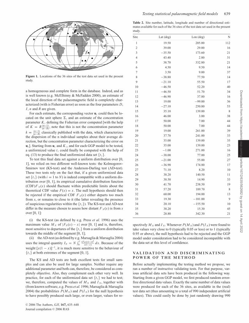
Figure 1. Locations of the 36 sites of the test data set used in the present
study.
a homogeneous and complete form in the database. Indeed, and as
is well known (e.g. McElhinny & McFadden 2000), an estimate of
the local direction of the palaeomagnetic field is completely char-
acterized (with is Fisherian error) as soon as the four parameters D,
I , n and R are given.
For each estimate, the corresponding vector ui could then be lo-
cated on the unit sphere �, and an estimate of the concentration
parameter K i defining the Fisherian error computed [with the help
of K = R (n−1)
(n−R); note that this is not the concentration parameter
k = (n−1)
(n−R)classically published with the data, which characterizes
the dispersion of the n individual samples about their average di-
rection, but the concentration parameter characterizing the error on
ui ]. Starting from ui and K i , and for each GGP model to be tested,
a uniformized value t i could finally be computed with the help of
eq. (13) to produce the final uniformized data set {t i}.
To test this final data set against a uniform distribution over [0,
1], we relied on two different well-known tests: the Kolmogorov-
Smirnov test (KS-test) and the Anderson-Darling test (AD-test).
These two tests rely on the fact that, if a given uniformized data
set {t i} (with i = 1 to N) is indeed compatible with a uniform dis-
tribution over [0, 1], its empirical cumulative distribution function
(CDF)F N (x) should fluctuate within predictable limits about the
theoretical CDF value F(x) = x . The null hypothesis should then
be rejected if the empirical CDF F N (x) either departs too much
from x, or remains to close to it (the latter revealing the presence
of suspicious regularities within the {t i}). The KS-test and AD-test
differ in the measure chosen to assess how distant F N (x) is from xover [0, 1]:
(i) the KS-test (as defined by e.g. Press et al. 1996) uses the
maximum value M N of |FN (x) − x | over [0, 1] and is, therefore,
most sensitive to departures of the {t i} from a uniform distribution
towards the middle of the segment [0, 1];
(ii) the AD-test (as defined by e.g. Marsaglia & Marsaglia 2004)
uses the integral quantity IN = N∫ 1
0(FN (x)−x)2
x(1−x)dx . Because of the
weight [x(1 − x)]−1, it is much more sensitive to the behaviour of
{t i} at both extremes of the segment [0, 1].
The KS and AD tests are both excellent tests for small sam-
ples and can also be used for large samples. Neither require any
additional parameter and both can, therefore, be considered as com-
pletely objective. Also, they complement each other very well. In
practice, for each of the uniformized data set {t i} we had to test;
we, therefore, computed the values of M N and I N , together with
(from known software, e.g. Press et al. 1996; Marsaglia & Marsaglia
2004) the probabilities P(M N ) and P(I N ) for the null hypothesis
to have possibly produced such large, or even larger, values for re-
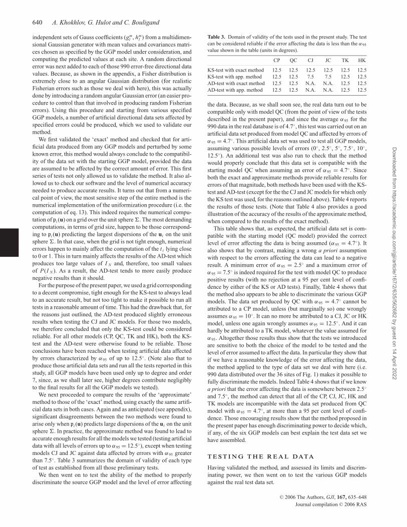
Table 2. Site number, latitude, longitude and number of directional esti-
mates available for each of the 36 sites of the test data set used in the present
study.
Site Lat (deg) Lon (deg) N
1 19.50 205.00 112
2 39.00 29.00 16
3 −35.50 173.60 21
4 43.40 2.80 31
5 38.70 332.80 21
6 4.50 9.50 14
7 3.50 9.00 37
8 −38.80 77.50 14
9 −21.10 55.50 17
10 −46.50 52.20 40
11 −46.50 51.70 34
12 −46.90 37.80 16
13 19.00 −99.00 36
14 −27.10 250.80 53
15 35.10 139.00 8
16 46.00 3.00 38
17 50.00 7.00 44
18 50.00 7.00 44
19 19.00 261.00 39
20 37.70 241.00 33
21 35.00 139.00 35
22 35.00 139.00 23
23 −1.00 271.00 16
24 −38.00 77.00 25
25 −21.00 55.00 27
26 −36.90 174.80 17
27 71.10 8.20 10
28 38.20 140.50 11
29 38.50 14.90 33
30 41.70 238.50 19
31 57.20 189.70 8
32 60.00 194.00 13
33 19.30 −101.00 9
34 20.10 −155.50 10
35 38.20 15.30 45
36 28.80 342.30 21
spectively M N and I N . Whenever P(M N ) and P(I N ) were found to
take values very close to 0 (typically 0.05 or less) or to 1 (typically
0.95 or above), the null hypothesis had to be rejected and the GGP
model under consideration had to be considered incompatible with
the data-set at this level of confidence.
VA L I DAT I O N A N D D I S C R I M I N AT I N G
P O W E R O F T H E M E T H O D
Before actually implementing the testing method we propose, we
ran a number of instructive validating tests. For that purpose, var-
ious artificial data sets have been produced in the following way.
Starting from a given GGP model, we first produced random error-
free directional data values. Exactly the same number of data values
were produced for each of the 36 sites, as available in the (real)
test data set (thus amounting to a total of 990 independent artificial
values). This could easily be done by just randomly drawing 990
C© 2006 The Authors, GJI, 167, 635–648
Journal compilation C© 2006 RAS
Dow
nloaded from https://academ
ic.oup.com/gji/article/167/2/635/562682 by guest on 14 April 2022
640 A. Khokhlov, G. Hulot and C. Bouligand
independent sets of Gauss coefficients (gml , hm
l ) from a multidimen-
sional Gaussian generator with mean values and covariances matri-
ces chosen as specified by the GGP model under consideration, and
computing the predicted values at each site. A random directional
error was next added to each of those 990 error-free directional data
values. Because, as shown in the appendix, a Fisher distribution is
extremely close to an angular Gaussian distribution (for realistic
Fisherian errors such as those we deal with here), this was actually
done by introducing a random angular Gaussian error (an easier pro-
cedure to control than that involved in producing random Fisherian
errors). Using this procedure and starting from various specified
GGP models, a number of artificial directional data sets affected by
specified errors could be produced, which we used to validate our
method.
We first validated the ‘exact’ method and checked that for arti-
ficial data produced from any GGP models and perturbed by some
known error, this method would always conclude to the compatibil-
ity of the data set with the starting GGP model, provided the data
are assumed to be affected by the correct amount of error. This first
series of tests not only allowed us to validate the method. It also al-
lowed us to check our software and the level of numerical accuracy
needed to produce accurate results. It turns out that from a numeri-
cal point of view, the most sensitive step of the entire method is the
numerical implementation of the uniformization procedure (i.e. the
computation of eq. 13). This indeed requires the numerical compu-
tation of pi (u) on a grid over the unit sphere �. The most demanding
computations, in terms of grid size, happen to be those correspond-
ing to pi (u) predicting the largest dispersions of the ui on the unit
sphere �. In that case, when the grid is not tight enough, numerical
errors happen to mainly affect the computation of the t i lying close
to 0 or 1. This in turn mainly affects the results of the AD-test which
produces too large values of I N and, therefore, too small values
of P(I N ). As a result, the AD-test tends to more easily produce
negative results than it should.
For the purpose of the present paper, we used a grid corresponding
to a decent compromise, tight enough for the KS-test to always lead
to an accurate result, but not too tight to make it possible to run all
tests in a reasonable amount of time. This had the drawback that, for
the reasons just outlined, the AD-test produced slightly erroneous
results when testing the CJ and JC models. For those two models,
we therefore concluded that only the KS-test could be considered
reliable. For all other models (CP, QC, TK and HK), both the KS-
test and the AD-test were otherwise found to be reliable. Those
conclusions have been reached when testing artificial data affected
by errors characterized by α95 of up to 12.5◦. (Note also that to
produce those artificial data sets and run all the tests reported in this
study, all GGP models have been used only up to degree and order
7, since, as we shall later see, higher degrees contribute negligibly
to the final results for all the GGP models we tested).
We next proceeded to compare the results of the ‘approximate’
method to those of the ‘exact’ method, using exactly the same artifi-
cial data sets in both cases. Again and as anticipated (see appendix),
significant disagreements between the two methods were found to
arise only when pi (u) predicts large dispersions of the ui on the unit
sphere �. In practice, the approximate method was found to lead to
accurate enough results for all the models we tested (testing artificial
data with all levels of errors up to α95 = 12.5◦), except when testing
models CJ and JC against data affected by errors with α95 greater
than 7.5◦. Table 3 summarizes the domain of validity of each type
of test as established from all those preliminary tests.
We then went on to test the ability of the method to properly
discriminate the source GGP model and the level of error affecting
Table 3. Domain of validity of the tests used in the present study. The test
can be considered reliable if the error affecting the data is less than the α95
value shown in the table (units in degrees).
CP QC CJ JC TK HK
KS-test with exact method 12.5 12.5 12.5 12.5 12.5 12.5
KS-test with app. method 12.5 12.5 7.5 7.5 12.5 12.5
AD-test with exact method 12.5 12.5 N.A. N.A. 12.5 12.5
AD-test with app. method 12.5 12.5 N.A. N.A. 12.5 12.5
the data. Because, as we shall soon see, the real data turn out to be
compatible only with model QC (from the point of view of the tests
described in the present paper), and since the average α95 for the
990 data in the real database is of 4.7◦, this test was carried out on an
artificial data set produced from model QC and affected by errors of
α95 = 4.7◦. This artificial data set was used to test all GGP models,
assuming various possible levels of errors (0◦, 2.5◦, 5◦, 7.5◦, 10◦,
12.5◦). An additional test was also run to check that the method
would properly conclude that this data set is compatible with the
starting model QC when assuming an error of α95 = 4.7◦. Since
both the exact and approximate methods provide reliable results for
errors of that magnitude, both methods have been used with the KS-
test and AD-test (except for the the CJ and JC models for which only
the KS test was used, for the reasons outlined above). Table 4 reports
the results of those tests. (Note that Table 4 also provides a good
illustration of the accuracy of the results of the approximate method,
when compared to the results of the exact method).
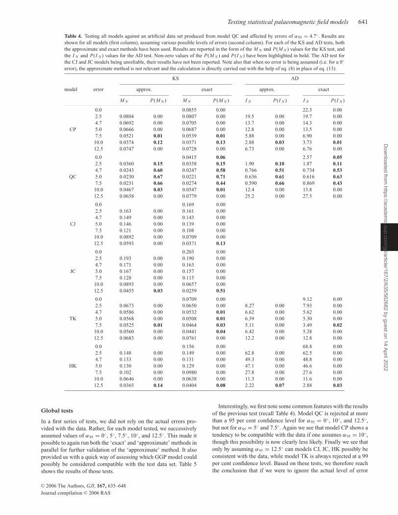
This table shows that, as expected, the artificial data set is com-
patible with the starting model (QC model) provided the correct
level of error affecting the data is being assumed (α95 = 4.7◦). It
also shows that by contrast, making a wrong a priori assumption
with respect to the errors affecting the data can lead to a negative
result. A minimum error of α95 = 2.5◦ and a maximum error of
α95 = 7.5◦ is indeed required for the test with model QC to produce
positive results (with no rejection at a 95 per cent level of confi-
dence by either of the KS or AD tests). Finally, Table 4 shows that
the method also appears to be able to discriminate the various GGP
models. The data set produced by QC with α95 = 4.7◦ cannot be
attributed to a CP model, unless (but marginally so) one wrongly
assumes α95 = 10◦. It can no more be attributed to a CJ, JC or HK
model, unless one again wrongly assumes α95 = 12.5◦. And it can
hardly be attributed to a TK model, whatever the value assumed for
α95. Altogether those results thus show that the tests we introduced
are sensitive to both the choice of the model to be tested and the
level of error assumed to affect the data. In particular they show that
if we have a reasonable knowledge of the error affecting the data,
the method applied to the type of data set we deal with here (i.e.
990 data distributed over the 36 sites of Fig. 1) makes it possible to
fully discriminate the models. Indeed Table 4 shows that if we know
a priori that the error affecting the data is somewhere between 2.5◦
and 7.5◦, the method can detect that all of the CP, CJ, JC, HK and
TK models are incompatible with the data set produced from QC
model with α95 = 4.7◦, at more than a 95 per cent level of confi-
dence. Those encouraging results show that the method proposed in
the present paper has enough discriminating power to decide which,
if any, of the six GGP models can best explain the test data set we
have assembled.
T E S T I N G T H E R E A L DATA
Having validated the method, and assessed its limits and discrim-
inating power, we then went on to test the various GGP models
against the real test data set.
C© 2006 The Authors, GJI, 167, 635–648
Journal compilation C© 2006 RAS
Dow
nloaded from https://academ
ic.oup.com/gji/article/167/2/635/562682 by guest on 14 April 2022
Testing statistical palaeomagnetic field models 641
Table 4. Testing all models against an artificial data set produced from model QC and affected by errors of α95 = 4.7◦. Results are
shown for all models (first column), assuming various possible levels of errors (second column). For each of the KS and AD tests, both
the approximate and exact methods have been used. Results are reported in the form of the M N and P(M N ) values for the KS test, and
the I N and P(I N ) values for the AD test. Non-zero values of the P(M N ) and P(I N ) have been highlighted in bold. The AD test for
the CJ and JC models being unreliable, their results have not been reported. Note also that when no error is being assumed (i.e. for a 0◦error), the approximate method is not relevant and the calculation is directly carried out with the help of eq. (8) in place of eq. (13).
KS AD
model error approx. exact approx. exact
M N P(M N ) M N P(M N ) I N P(I N ) I N P(I N )
0.0 0.0855 0.00 22.3 0.00
2.5 0.0804 0.00 0.0807 0.00 19.5 0.00 19.7 0.00
4.7 0.0692 0.00 0.0705 0.00 13.7 0.00 14.3 0.00
CP 5.0 0.0666 0.00 0.0687 0.00 12.8 0.00 13.5 0.00
7.5 0.0521 0.01 0.0539 0.01 5.88 0.00 6.90 0.00
10.0 0.0374 0.12 0.0371 0.13 2.88 0.03 3.73 0.0112.5 0.0747 0.00 0.0728 0.00 6.73 0.00 6.76 0.00
0.0 0.0415 0.06 2.57 0.052.5 0.0360 0.15 0.0358 0.15 1.90 0.10 1.87 0.114.7 0.0243 0.60 0.0247 0.58 0.766 0.51 0.734 0.53
QC 5.0 0.0230 0.67 0.0221 0.71 0.636 0.61 0.616 0.637.5 0.0231 0.66 0.0274 0.44 0.590 0.66 0.869 0.4310.0 0.0467 0.03 0.0547 0.01 12.4 0.00 13.8 0.00
12.5 0.0658 0.00 0.0779 0.00 25.2 0.00 27.5 0.00
0.0 0.169 0.00
2.5 0.163 0.00 0.161 0.00
4.7 0.149 0.00 0.143 0.00
CJ 5.0 0.146 0.00 0.139 0.00
7.5 0.121 0.00 0.108 0.00
10.0 0.0892 0.00 0.0709 0.00
12.5 0.0593 0.00 0.0371 0.13
0.0 0.203 0.00
2.5 0.193 0.00 0.190 0.00
4.7 0.171 0.00 0.163 0.00
JC 5.0 0.167 0.00 0.157 0.00
7.5 0.128 0.00 0.115 0.00
10.0 0.0893 0.00 0.0657 0.00
12.5 0.0455 0.03 0.0259 0.51
0.0 0.0709 0.00 9.12 0.00
2.5 0.0673 0.00 0.0650 0.00 8.27 0.00 7.93 0.00
4.7 0.0586 0.00 0.0532 0.01 6.62 0.00 5.62 0.00
TK 5.0 0.0568 0.00 0.0508 0.01 6.39 0.00 5.30 0.00
7.5 0.0525 0.01 0.0464 0.03 5.11 0.00 3.49 0.0210.0 0.0560 0.00 0.0441 0.04 6.42 0.00 5.28 0.00
12.5 0.0683 0.00 0.0761 0.00 12.2 0.00 12.8 0.00
0.0 0.156 0.00 68.8 0.00
2.5 0.148 0.00 0.149 0.00 62.8 0.00 62.5 0.00
4.7 0.133 0.00 0.131 0.00 49.3 0.00 48.8 0.00
HK 5.0 0.130 0.00 0.129 0.00 47.1 0.00 46.6 0.00
7.5 0.102 0.00 0.0980 0.00 27.8 0.00 27.6 0.00
10.0 0.0646 0.00 0.0638 0.00 11.3 0.00 11.6 0.00
12.5 0.0365 0.14 0.0404 0.08 2.22 0.07 2.88 0.03
Global tests
In a first series of tests, we did not rely on the actual errors pro-
vided with the data. Rather, for each model tested, we successively
assumed values of α95 = 0◦, 5◦, 7.5◦, 10◦, and 12.5◦. This made it
possible to again run both the ‘exact’ and ‘approximate’ methods in
parallel for further validation of the ‘approximate’ method. It also
provided us with a quick way of assessing which GGP model could
possibly be considered compatible with the test data set. Table 5
shows the results of those tests.
Interestingly, we first note some common features with the results
of the previous test (recall Table 4). Model QC is rejected at more
than a 95 per cent confidence level for α95 = 0◦, 10◦, and 12.5◦,
but not for α95 = 5◦ and 7.5◦. Again we see that model CP shows a
tendency to be compatible with the data if one assumes α95 = 10◦,
though this possibility is now clearly less likely. Finally we see that
only by assuming α95 = 12.5◦ can models CJ, JC, HK possibly be
consistent with the data, while model TK is always rejected at a 99
per cent confidence level. Based on these tests, we therefore reach
the conclusion that if we were to ignore the actual level of error
C© 2006 The Authors, GJI, 167, 635–648
Journal compilation C© 2006 RAS
Dow
nloaded from https://academ
ic.oup.com/gji/article/167/2/635/562682 by guest on 14 April 2022
642 A. Khokhlov, G. Hulot and C. Bouligand
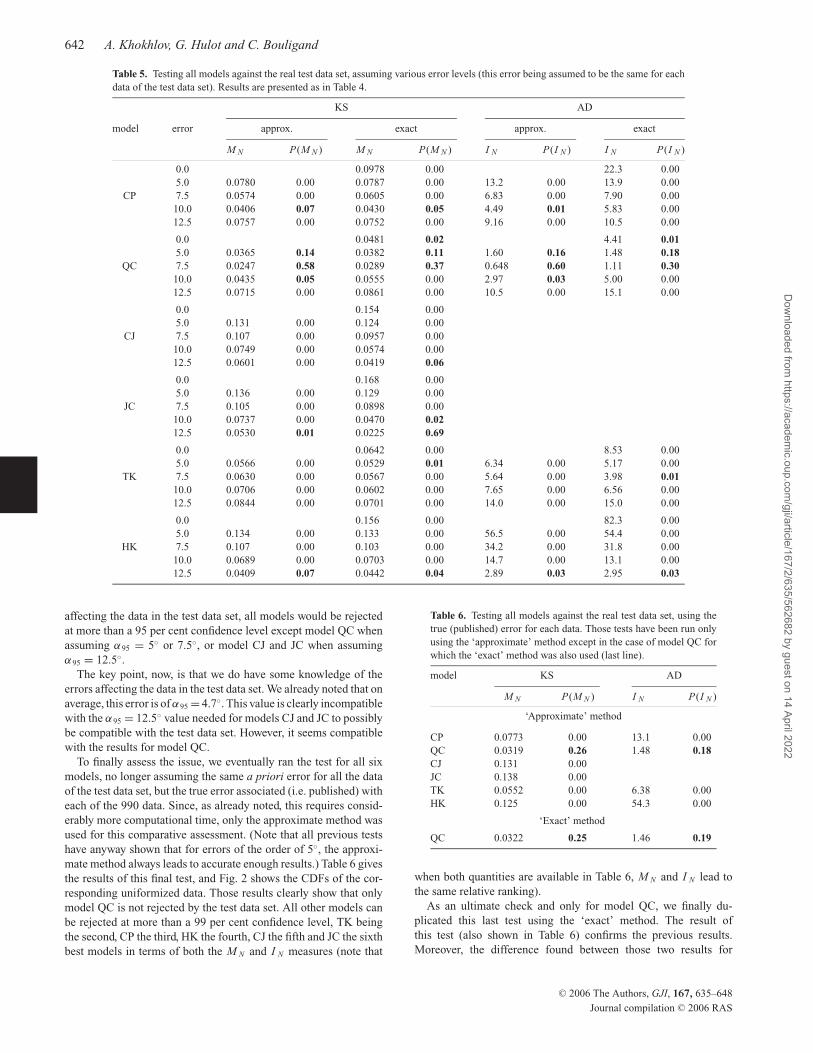
Table 5. Testing all models against the real test data set, assuming various error levels (this error being assumed to be the same for each
data of the test data set). Results are presented as in Table 4.
KS AD
model error approx. exact approx. exact
M N P(M N ) M N P(M N ) I N P(I N ) I N P(I N )
0.0 0.0978 0.00 22.3 0.00
5.0 0.0780 0.00 0.0787 0.00 13.2 0.00 13.9 0.00
CP 7.5 0.0574 0.00 0.0605 0.00 6.83 0.00 7.90 0.00
10.0 0.0406 0.07 0.0430 0.05 4.49 0.01 5.83 0.00
12.5 0.0757 0.00 0.0752 0.00 9.16 0.00 10.5 0.00
0.0 0.0481 0.02 4.41 0.015.0 0.0365 0.14 0.0382 0.11 1.60 0.16 1.48 0.18
QC 7.5 0.0247 0.58 0.0289 0.37 0.648 0.60 1.11 0.3010.0 0.0435 0.05 0.0555 0.00 2.97 0.03 5.00 0.00
12.5 0.0715 0.00 0.0861 0.00 10.5 0.00 15.1 0.00
0.0 0.154 0.00
5.0 0.131 0.00 0.124 0.00
CJ 7.5 0.107 0.00 0.0957 0.00
10.0 0.0749 0.00 0.0574 0.00
12.5 0.0601 0.00 0.0419 0.06
0.0 0.168 0.00
5.0 0.136 0.00 0.129 0.00
JC 7.5 0.105 0.00 0.0898 0.00
10.0 0.0737 0.00 0.0470 0.0212.5 0.0530 0.01 0.0225 0.69
0.0 0.0642 0.00 8.53 0.00
5.0 0.0566 0.00 0.0529 0.01 6.34 0.00 5.17 0.00
TK 7.5 0.0630 0.00 0.0567 0.00 5.64 0.00 3.98 0.0110.0 0.0706 0.00 0.0602 0.00 7.65 0.00 6.56 0.00
12.5 0.0844 0.00 0.0701 0.00 14.0 0.00 15.0 0.00
0.0 0.156 0.00 82.3 0.00
5.0 0.134 0.00 0.133 0.00 56.5 0.00 54.4 0.00
HK 7.5 0.107 0.00 0.103 0.00 34.2 0.00 31.8 0.00
10.0 0.0689 0.00 0.0703 0.00 14.7 0.00 13.1 0.00
12.5 0.0409 0.07 0.0442 0.04 2.89 0.03 2.95 0.03
affecting the data in the test data set, all models would be rejected
at more than a 95 per cent confidence level except model QC when
assuming α95 = 5◦ or 7.5◦, or model CJ and JC when assuming
α95 = 12.5◦.
The key point, now, is that we do have some knowledge of the
errors affecting the data in the test data set. We already noted that on
average, this error is of α95 = 4.7◦. This value is clearly incompatible
with the α95 = 12.5◦ value needed for models CJ and JC to possibly
be compatible with the test data set. However, it seems compatible
with the results for model QC.
To finally assess the issue, we eventually ran the test for all six
models, no longer assuming the same a priori error for all the data
of the test data set, but the true error associated (i.e. published) with
each of the 990 data. Since, as already noted, this requires consid-
erably more computational time, only the approximate method was
used for this comparative assessment. (Note that all previous tests
have anyway shown that for errors of the order of 5◦, the approxi-
mate method always leads to accurate enough results.) Table 6 gives
the results of this final test, and Fig. 2 shows the CDFs of the cor-
responding uniformized data. Those results clearly show that only
model QC is not rejected by the test data set. All other models can
be rejected at more than a 99 per cent confidence level, TK being
the second, CP the third, HK the fourth, CJ the fifth and JC the sixth
best models in terms of both the M N and I N measures (note that
Table 6. Testing all models against the real test data set, using the
true (published) error for each data. Those tests have been run only
using the ‘approximate’ method except in the case of model QC for
which the ‘exact’ method was also used (last line).
model KS AD
M N P(M N ) I N P(I N )
‘Approximate’ method
CP 0.0773 0.00 13.1 0.00
QC 0.0319 0.26 1.48 0.18CJ 0.131 0.00
JC 0.138 0.00
TK 0.0552 0.00 6.38 0.00
HK 0.125 0.00 54.3 0.00
‘Exact’ method
QC 0.0322 0.25 1.46 0.19
when both quantities are available in Table 6, M N and I N lead to
the same relative ranking).
As an ultimate check and only for model QC, we finally du-
plicated this last test using the ‘exact’ method. The result of
this test (also shown in Table 6) confirms the previous results.
Moreover, the difference found between those two results for
C© 2006 The Authors, GJI, 167, 635–648
Journal compilation C© 2006 RAS
Dow
nloaded from https://academ
ic.oup.com/gji/article/167/2/635/562682 by guest on 14 April 2022
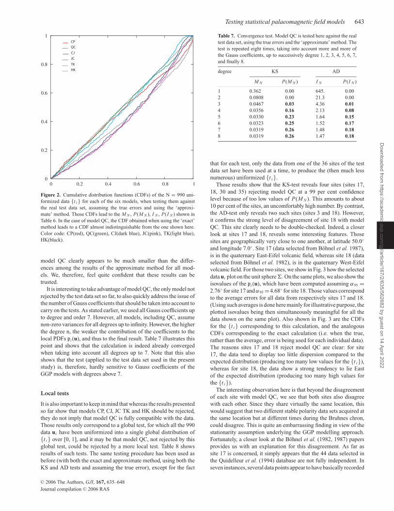
Testing statistical palaeomagnetic field models 643
CP
QC
CJ
JC
TK
HK
Figure 2. Cumulative distribution functions (CDFs) of the N = 990 uni-
formized data {t i} for each of the six models, when testing them against
the real test data set, assuming the true errors and using the ‘approxi-
mate’ method. Those CDFs lead to the M N , P(M N ), I N , P(I N ) shown in
Table 6. In the case of model QC, the CDF obtained when using the ‘exact’
method leads to a CDF almost indistinguishable from the one shown here.
Color code: CP(red), QC(green), CJ(dark blue), JC(pink), TK(light blue),
HK(black).
model QC clearly appears to be much smaller than the differ-
ences among the results of the approximate method for all mod-
els. We, therefore, feel quite confident that these results can be
trusted.
It is interesting to take advantage of model QC, the only model not
rejected by the test data set so far, to also quickly address the issue of
the number of Gauss coefficients that should be taken into account to
carry on the tests. As stated earlier, we used all Gauss coefficients up
to degree and order 7. However, all models, including QC, assume
non-zero variances for all degrees up to infinity. However, the higher
the degree n, the weaker the contribution of the coefficients to the
local PDFs pi (u), and thus to the final result. Table 7 illustrates this
point and shows that the calculation is indeed already converged
when taking into account all degrees up to 7. Note that this also
shows that the test (applied to the test data set used in the present
study) is, therefore, hardly sensitive to Gauss coefficients of the
GGP models with degrees above 7.
Local tests
It is also important to keep in mind that whereas the results presented
so far show that models CP, CJ, JC TK and HK should be rejected,
they do not imply that model QC is fully compatible with the data.
Those results only correspond to a global test, for which all the 990
data ui have been uniformized into a single global distribution of
{t i} over [0, 1], and it may be that model QC, not rejected by this
global test, could be rejected by a more local test. Table 8 shows
results of such tests. The same testing procedure has been used as
before (with both the exact and approximate method, using both the
KS and AD tests and assuming the true error), except for the fact
Table 7. Convergence test. Model QC is tested here against the real
test data set, using the true errors and the ‘approximate’ method. The
test is repeated eight times, taking into account more and more of
the Gauss coefficients, up to successively degree 1, 2, 3, 4, 5, 6, 7,
and finally 8.
degree KS AD
M N P(M N ) I N P(I N )
1 0.362 0.00 645. 0.00
2 0.0808 0.00 21.3 0.00
3 0.0467 0.03 4.36 0.014 0.0356 0.16 2.13 0.085 0.0330 0.23 1.64 0.156 0.0323 0.25 1.52 0.177 0.0319 0.26 1.48 0.188 0.0319 0.26 1.47 0.18
that for each test, only the data from one of the 36 sites of the test
data set have been used at a time, to produce the (then much less
numerous) uniformized {t i}.
Those results show that the KS-test reveals four sites (sites 17,
18, 30 and 35) rejecting model QC at a 99 per cent confidence
level because of too low values of P(M N ). This amounts to about
10 per cent of the sites, an uncomfortably high number. By contrast,
the AD-test only reveals two such sites (sites 3 and 18). However,
it confirms the strong level of disagreement of site 18 with model
QC. This site clearly needs to be double-checked. Indeed, a closer
look at sites 17 and 18, reveals some interesting features. Those
sites are geographically very close to one another, at latitude 50.0◦
and longitude 7.0◦. Site 17 (data selected from Bohnel et al. 1987),
is in the quaternary East-Eifel volcanic field, whereas site 18 (data
selected from Bohnel et al. 1982), is in the quaternary West-Eifel
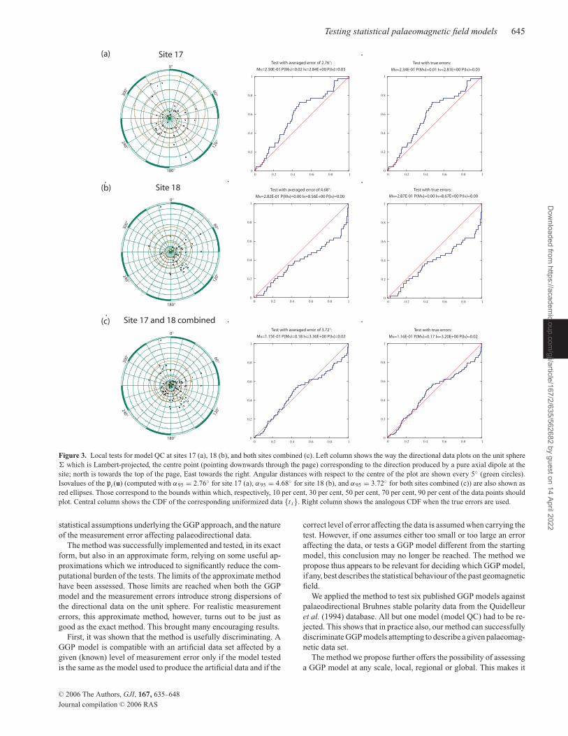
volcanic field. For those two sites, we show in Fig. 3 how the selected
data ui plot on the unit sphere �. On the same plots, we also show the
isovalues of the pi (u), which have been computed assuming α95 =2.76◦ for site 17 and α95 = 4.68◦ for site 18. Those values correspond
to the average errors for all data from respectively sites 17 and 18.
(Using such averages is done here mainly for illustrative purpose, the
plotted isovalues being then simultaneously meaningful for all the
data shown on the same plot). Also shown in Fig. 3 are the CDFs
for the {t i} corresponding to this calculation, and the analogous
CDFs corresponding to the exact calculation (i.e. when the true,
rather than the average, error is being used for each individual data).
The reasons sites 17 and 18 reject model QC are clear: for site
17, the data tend to display too little dispersion compared to the
expected distribution (producing too many low values for the {t i}),
whereas for site 18, the data show a strong tendency to lie East
of the expected distribution (producing too many high values for
the {t i}).
The interesting observation here is that beyond the disagreement
of each site with model QC, we see that both sites also disagree
with each other. Since they share virtually the same location, this
would suggest that two different stable polarity data sets acquired at
the same location but at different times during the Bruhnes chron,
could disagree. This is quite an embarrassing finding in view of the
stationarity assumption underlying the GGP modelling approach.
Fortunately, a closer look at the Bohnel et al. (1982, 1987) papers
provides us with an explanation for this disagreement. As far as
site 17 is concerned, it simply appears that the 44 data selected in
the Quidelleur et al. (1994) database are not fully independent. In
seven instances, several data points appear to have basically recorded
C© 2006 The Authors, GJI, 167, 635–648
Journal compilation C© 2006 RAS
Dow
nloaded from https://academ
ic.oup.com/gji/article/167/2/635/562682 by guest on 14 April 2022

644 A. Khokhlov, G. Hulot and C. Bouligand
Table 8. Testing model QC against the real test data set on a site by site basis. The true errors and both the ‘approximate’ and ‘exact’
methods are being used. For each site, results are provided for both the KS and AD tests.
KS AD
Site Approx. Exact Approx. Exact
M N P(M N ) M N P(M N ) I N P(I N ) I N P(I N )
1 0.106 0.15 0.105 0.16 1.81 0.12 1.73 0.13
2 0.149 0.84 0.163 0.75 0.626 0.62 0.598 0.65
3 0.284 0.05 0.286 0.05 3.63 0.01 3.63 0.01
4 0.106 0.86 0.105 0.86 0.485 0.76 0.478 0.77
5 0.122 0.90 0.115 0.93 0.576 0.67 0.542 0.70
6 0.162 0.82 0.162 0.82 1.01 0.35 0.991 0.36
7 0.0745 0.98 0.0762 0.98 0.401 0.85 0.413 0.83
8 0.288 0.16 0.287 0.16 2.96 0.03 2.92 0.03
9 0.265 0.15 0.264 0.16 1.28 0.24 1.27 0.24
10 0.208 0.05 0.211 0.05 3.46 0.02 3.33 0.02
11 0.167 0.27 0.165 0.29 1.46 0.19 1.46 0.19
12 0.199 0.50 0.198 0.51 0.469 0.78 0.458 0.79
13 0.156 0.32 0.158 0.30 2.08 0.08 2.23 0.07
14 0.0867 0.80 0.0878 0.79 0.686 0.57 0.625 0.62
15 0.304 0.38 0.325 0.30 2.71 0.04 2.88 0.03
16 0.116 0.66 0.108 0.74 0.876 0.43 0.789 0.49
17 0.234 0.01 0.233 0.01 2.81 0.03 2.83 0.03
18 0.287 0.00 0.288 0.00 8.67 0.00 8.76 0.00
19 0.185 0.12 0.195 0.09 2.31 0.06 2.49 0.05
20 0.136 0.55 0.136 0.54 0.618 0.63 0.614 0.63
21 0.212 0.07 0.201 0.10 1.88 0.11 1.67 0.14
22 0.200 0.28 0.198 0.30 1.77 0.12 1.85 0.11
23 0.199 0.51 0.199 0.50 1.08 0.32 1.08 0.32
24 0.147 0.62 0.158 0.52 1.79 0.12 1.91 0.10
25 0.198 0.21 0.199 0.21 2.41 0.06 2.48 0.05
26 0.0941 1.00 0.0916 1.00 0.301 0.94 0.315 0.93
27 0.222 0.65 0.239 0.56 0.796 0.48 0.846 0.45
28 0.368 0.08 0.373 0.07 2.64 0.04 2.79 0.04
29 0.140 0.50 0.141 0.50 0.908 0.41 0.994 0.36
30 0.364 0.01 0.357 0.01 2.52 0.05 2.43 0.05
31 0.327 0.30 0.321 0.32 1.64 0.15 1.64 0.15
32 0.179 0.76 0.179 0.76 1.45 0.19 1.40 0.20
33 0.209 0.78 0.210 0.77 0.925 0.40 0.927 0.40
34 0.273 0.38 0.274 0.38 1.47 0.19 1.45 0.19
35 0.248 0.01 0.240 0.01 3.42 0.02 3.23 0.02
36 0.119 0.91 0.112 0.94 0.480 0.77 0.455 0.79
the same field (each time reflecting a single volcanic event). Those
events correspond to low values of t i and bias the distribution of
the {t i} towards low values. Site 18 is a slightly different story. In
that case, Bohnel et al. (1987) make a good case that a subset of
the data they published must have recorded a relatively short-lived
excursion or event during the Bruhnes chron, biasing the data set
towards the East. Although Quidelleur et al. (1994) rejected most
of those transitional data (based on the selection criteria that the
data must correspond to a period of stable polarity) some of the data
biased towards that transitional direction have clearly been included
within the database. Thus the issue with sites 17 and 18 appears to
be more one of ill sampling than one of overall disagreement with
model QC. Interestingly, we further note that if we actually bin the
two sites into a single one, as is also shown in Fig. 3, the local test no
longer rejects model QC. This then leaves only two sites (30 and 35)
out of 36 truly rejecting model QC at a 99 per cent confidence level
because of too low values of P(M N ), and only one site (site 3) reject-
ing QC because of a too low value of P(I N ). These are no longer
unexpected proportions and model QC thus indeed appears to be
compatible with the Quidelleur et al. (1994) Bruhnes stable polarity
data set.
C O N C L U S I O N
In the present paper we introduced the first quantitative method
capable of assessing the compatibility of a GGP model with a
given palaeodirectional database in a way consistent with both the
C© 2006 The Authors, GJI, 167, 635–648
Journal compilation C© 2006 RAS
Dow
nloaded from https://academ
ic.oup.com/gji/article/167/2/635/562682 by guest on 14 April 2022
Testing statistical palaeomagnetic field models 645
Site 17
Site 18
Site 17 and 18 combined
0°
60°
120°
180°
240°
300°
0°
60°
120°
120°
180°
180°
240°240°
300°
300°
0°
60°
Test with averaged error of 2.76°: Test with true errors:
MN=2.30E-01 P(MN)=0.02 IN=2.84E+00 P(IN)=0.03 MN=2.34E-01 P(MN)=0.01 IN=2.81E+00 P(IN)=0.03
Test with true errors:
MN=2.87E-01 P(MN)=0.00 IN=8.67E+00 P(IN)=0.00
Test with averaged error of 4.68°:
MN=2.82E-01 P(MN)=0.00 IN=8.56E+00 P(IN)=0.00
Test with averaged error of 3.72°:
MN=1.15E-01 P(MN)=0.18 IN=3.36E+00 P(IN)=0.02
Test with true errors:
MN=1.16E-01 P(MN)=0.17 IN=3.20E+00 P(IN)=0.02
(a)
(b)
(c)
Figure 3. Local tests for model QC at sites 17 (a), 18 (b), and both sites combined (c). Left column shows the way the directional data plots on the unit sphere
� which is Lambert-projected, the centre point (pointing downwards through the page) corresponding to the direction produced by a pure axial dipole at the
site; north is towards the top of the page, East towards the right. Angular distances with respect to the centre of the plot are shown every 5◦ (green circles).
Isovalues of the pi (u) (computed with α95 = 2.76◦ for site 17 (a), α95 = 4.68◦ for site 18 (b), and α95 = 3.72◦ for both sites combined (c)) are also shown as
red ellipses. Those correspond to the bounds within which, respectively, 10 per cent, 30 per cent, 50 per cent, 70 per cent, 90 per cent of the data points should
plot. Central column shows the CDF of the corresponding uniformized data {t i}. Right column shows the analogous CDF when the true errors are used.
statistical assumptions underlying the GGP approach, and the nature
of the measurement error affecting palaeodirectional data.
The method was successfully implemented and tested, in its exact
form, but also in an approximate form, relying on some useful ap-
proximations which we introduced to significantly reduce the com-
putational burden of the tests. The limits of the approximate method
have been assessed. Those limits are reached when both the GGP
model and the measurement errors introduce strong dispersions of
the directional data on the unit sphere. For realistic measurement
errors, this approximate method, however, turns out to be just as
good as the exact method. This brought many encouraging results.
First, it was shown that the method is usefully discriminating. A
GGP model is compatible with an artificial data set affected by a
given (known) level of measurement error only if the model tested
is the same as the model used to produce the artificial data and if the
correct level of error affecting the data is assumed when carrying the
test. However, if one assumes either too small or too large an error
affecting the data, or tests a GGP model different from the starting
model, this conclusion may no longer be reached. The method we
propose thus appears to be relevant for deciding which GGP model,
if any, best describes the statistical behaviour of the past geomagnetic
field.
We applied the method to test six published GGP models against
palaeodirectional Bruhnes stable polarity data from the Quidelleur
et al. (1994) database. All but one model (model QC) had to be re-
jected. This shows that in practice also, our method can successfully
discriminate GGP models attempting to describe a given palaeomag-
netic data set.
The method we propose further offers the possibility of assessing
a GGP model at any scale, local, regional or global. This makes it
C© 2006 The Authors, GJI, 167, 635–648
Journal compilation C© 2006 RAS
Dow
nloaded from https://academ
ic.oup.com/gji/article/167/2/635/562682 by guest on 14 April 2022
646 A. Khokhlov, G. Hulot and C. Bouligand
possible to better scrutinize a GGP model which first passed tests at
a global scale. Any disagreement between the prediction of the GGP
model and the data set at a local level can then be used to double-
check not only the GGP model, but also the data set itself. Applying
this checking procedure to model QC allowed us to identify such
problems with two sites of the Quidelleur et al. (1994) database and
to confirm the compatibility of this model with the rest of the test
data set.
This success of at least one GGP model is motivating. It shows, for
the first time, that the statistical behaviour of the geomagnetic field
at times of stable polarity can indeed be described in a consistent
way in terms of a GGP model. However, the specific success of
model QC should not be overemphasized. This model was inferred
in an empirical way by Quidelleur & Courtillot (1996) from the
Quidelleur et al. (1994) database from which our test data set was
also extracted. All other models were inferred (also in empirical
ways) from different databases, and even though all those databases
share many common data, they may very well not be fully compatible
with each other and with our own data set. Part of the failure of
those GGP models at being compatible with our test data set might
originate from this. With this respect, it is quite clear that finally
confirming the success of the QC model (and the failure of other
models) would still require a more thorough study, involving a more
recent, extensive and independently assessed data set, extracted from
databases such as the IAGA palaeomagnetic reference database we
mentioned early on.
As a matter of fact, it is interesting to note that such a data set
could also include palaeointensity data extracted from databases
such as the IAGA palaeointensity reference database (PINT, Perrin
& Schnepp (2004)). Indeed, although the present paper mainly de-
scribed the way to deal with palaeodirectional data, palaeointensity
data could easily be taken into account [if such data provide the
full 3-D palaeofield at a given location, the way those data plot in
3-D can be compared with the local 3-D Gaussian statistics pre-
dicted by the GGP model (i.e. g) by using just the same kind of
uniformization procedure as the one we described, see paper I; and
taking measurement error into account would just consist in making
use of a modified, but still Gaussian, 3-D statistics of the type ga as
defined in the appendix, where ge is then directly the Gaussian error
assumed to affect the data]. In fact such tests might eventually show
that model QC also is incompatible with such a more complete data
set. However, if such is the case, the method we propose here could
be used to seek yet another model. Several strategies could then be
pursued. One could involve using the same kind of empirical proce-
dure as those used by Quidelleur & Courtillot (1996) to first guess
which parameter of the GGP model should be changed, and using
our method to assess the improvement brought. Another strategy,
more advanced and much more far fetched at this point, could in-
volve designing a more systematic ‘inverse’ approach based on the
present ‘forward’ testing method. In either case, however, several
issues would still have to be faced. In particular, we mentioned the
fact that the method is not sensitive to parameters corresponding
to degrees above 7, which reflects the weak contribution of those
high degrees to the geomagnetic field observed at the Earth’s sur-
face. However, we did not investigate in detail the sensitivity of
our test to the various parameters defining the mean field (E(k))
and the covariance matrix (Cov(k, k)) of a GGP model. Assessing
this would help us better understand how complex a GGP model,
and in particular its mean field, really needs to be to explain the
data. For the time being, and as far as the present test study can
suggest, the Bruhnes stable polarity data does not seem to call for
more complex a model than model QC: a mean field with only
a g01 and a weak g0
2 contribution, and a simple diagonal covari-
ance matrix only involving an enhanced σ 12 contribution along the
lines first suggested by Kono & Tanaka (1995) and Hulot & Gallet
(1996).
We plan to make our software available upon request (please be
in touch with the corresponding author: [email protected]) .
A C K N O W L E D G M E N T S
We thank Richard Holme and two anonymous reviewers for their
constructive comments. This is IPGP contribution 2147.
R E F E R E N C E S
Bingham, C., 1983. A series expansion for Angular Gaussian Distribution.
Appendix C., in Statistics on Spheres, ed. Watson, G., Wiley-Interscience
Pub., New York.
Bohnel, H., Kohnen, H., Negendank, J. & Schmincke, H.-U., 1982. Palaeo-
magnetism of Quaternary volcanics of the East-Eifel, Germany, J. Geo-phys., 51, 29–37.
Bohnel, H., Reismann, N., Jager, G., Haverkamp, U., Negendank, J.F.W.
& Schmincke, H.-U., 1987. Paleomagnetic investigation of Quaternary
West Eifel volcanics (Germany): indication for increased volcanic activity
during geomagnetic excursion/event?, J. Geophys., 62, 50–61.
Bouligand, C., Hulot, G., Khokhlov, A. & Glatzmaier, G.A., 2005. Statis-
tical paleomagnetic field modelling and dynamo numerical simulation,
Geophys. J. Int., 161, 603–626.
Constable, C.G. & Parker, R.L., 1988. Statistics of the geomagnetic secular
variation for the past 5 Myr, J. geophys. Res., 93, 11 569–11 581.
Constable, C.G. & Johnson, C.L., 1999. Anisotropic paleosecular variation
models: implications for geomagnetic field observables, Earth planet. Sci.Lett., 115, 35–51.
Hatakeyama, T. & Kono, M., 2001. Shift of the mean magnetic field values;
effect of scatter due to secular variation and errors, Earth Planets Space,53, 31–44.
Hatakeyama, T. & Kono, M., 2002. Geomagnetic field model for the last
5 Myr; time-averaged field and secular variation, Paleosecular variation
and reversals of the Earth’s magnetic field, Phys. Earth planet. Int., 133,181–215.
Hongre, L., Hulot, G. & Khokhlov, A., 1998. An analysis of the geomagnetic
field over the past 2000 years, Phys. Earth planet. Int., 106, 311–315.
Hulot, G. & Gallet, Y., 1996. On the interpretation of virtual geomagnetic
pole (VGP) scatter curves, Phys. Earth planet. Int., 95, 37–53.
Hulot, G. & Le Mouel, J.-L., 1994. A statistical approach to the Earth’s main
magnetic field, Phys. Earth planet. Int., 82, 167–183.
Hulot, G. & Bouligand, C., 2005. Statistical paleomagnetic field modelling
and symmetry considerations, Geophys. J. Int., 161, 591–602.
Hulot, G., Eymin, C., Langlais, B., Mandea, M. & Olsen, N., 2002.
Smallscale structure of the geodynamo inferred from Oersted and Magsat
satellite data, Nature, 416, 620–623.
Jackson, A., Jonkers, A.R.T. & Walker, M.R., 2000. Four centuries of ge-
omagnetic secular variation from historical records, Phil. Trans. R. Soc.Lond., A., 358, 957–990.
Johnson, C. & Constable, C., 1996. Paleosecular variation recorded by lava
flows over the last 5 Myr, Phil. Trans. R. Soc. Lond., 354, 89–141.
Khokhlov, A., Hulot, G. & Carlut, J., 2001. Towards a self-consistent ap-
proach to paleomagnetic field modelling, J. Int. Geoph., 145, 157–171.
Kono, M. & Tanaka, H., 1995. Mapping the Gauss coefficients to the pole and
the models of paleosecular variation, J. Geomag. Geoelectr., 47, 115–130.
Kono, M., Tanaka, H. & Tsukanawa, H., 2000a. Spherical harmonic analysis
of paleomagnetic data: the case of linear mapping, J. geophys. Res., 105,5817–5833.
Kono, M., Sakuraba, A. & Ishida, M., 2000b. Dynamo simulations and
paleosecular variation models, Phil. Trans. R. Soc. Lond., A, 358, 1123–
1139.
C© 2006 The Authors, GJI, 167, 635–648
Journal compilation C© 2006 RAS
Dow
nloaded from https://academ
ic.oup.com/gji/article/167/2/635/562682 by guest on 14 April 2022
Testing statistical palaeomagnetic field models 647
Korte, M. & Constable, C.G., 2005. Continuous geomagnetic field models
for the past 7 millennia: 2. CALS7K Geochem. Geophys. Geosys., 6,2004GC000801.
Love, J.J. & Constable, C.G., 2003. Gaussian statistics for paleomagnetic
vectors, Geophys. J. Int., 152, 515–565.
Marsaglia, G. & Marsaglia, J.C.W., 2004. Evaluating the Anderson-Darling
distribution, Journal Statistical Software, 9, Issue 5.
McElhinny, M. & McFadden, P., 1997. Paleosecular variation over the past
5Myr based on a new generalized database, Geophys. J. Int., 131, 240–252.
McElhinny, M. & McFadden, P., 2000. Paleomagnetism, Continents and
oceans, International Geophysics Series, 73, Academic Press, San Diego,
CA, USA.
McMillan, D.G., Constable, C.G., Parker, R.L. & Glatzmaier, G.A., 2001. A
statistical analysis of magnetic fields from some geodynamo simulations,
Geochem. Geophys. Geosys., 2, 2000GC000130.
Merrill, R., McElhinny, M. & McFadden, P., 1996. The Magnetic Field ofthe Earth, Academic Press, London.
Perrin, M. & Schnepp, E., 2004. IAGA paleointensity database: distribution
and quality of the data set, Phys. Earth planet. Int., 147, 255–267.
Press, C., Teukolsky, S., Vetterling, W. & Flannery, B., 1996. Numeri-
cal Recipes in C. 2nd edn, Cambridge, see also http://library.lanl.gov/
numerical/index.html.
Quidelleur, X. & Courtillot, V., 1996. On low-degree spherical harmonic
models of paleosecular variation, Phys. Earth planet. Int., 95, 55–77.
Quidelleur, X., Valet, J.-P., Courtillot, V. & Hulot, G., 1994. Long-term ge-
ometry of the geomagnetic field for the last five million years: an updated
secular variation database, Geophys. Res. Lett., 15, 1639–1642.
Tanaka, H., Kono, M. & Uchimura, H., 1995. Some global features of pale-
ointensity in geological time, Geophys. J. Int., 120, 97–102.
Tauxe, L., 2005. Inclination flattening and the geocentric axial dipole, Earthplanet. Sci. Lett., 233, 247–261.
Tauxe, L. & Kent, D.V., 2004. A simplified statistical model for the geomag-
netic field and the detection of shallow bias in paleomagnetic inclinations:
was the ancient magnetic field dipolar?, in Timescales of the Paleomag-netic field,Vol. 145, pp. 101–115. eds Channell, J.E.T., Kent, D.V., Lowrie,
W. & Meert, J., Am. Geophys. Un. Monongr.
A P P E N D I X : I N T RO D U C I N G U S E F U L
A N A LY T I C A P P RO X I M AT I O N S
Fisher and Angular Gaussian distributions
Let us first note that a Fisher distribution kK (u, s) centred on u ∈� with concentration parameter K is very close (when K is large
enough) to the angular Gaussian distribution derived from a 3-D
Gaussian distribution characterized by m and�i j =σ−2 δij , provided
u = m/|m| and σ = |m|K − 12 . This fairly intuitive result (see also
Love & Constable 2003), is in the same line as the better known
result that a Fisher distribution is very close to a 2-D Gaussian
distribution within the plane tangent to � at u (see e.g. Merrill et al.1996).
In spherical coordinates, and when assuming the Fisher distribu-
tion centred on u0 = (θ = 0, ϕ = 0), from eq. (7) we infer z =
Table A1. Departure ε(P) (as defined by A5) of the probability P predicted by the angular Gaussian distribution from that of the Fisher
distribution it approximates, for various values of P and of the concentration parameter K (and corresponding α95 values).
K α {0.95} ε(0.1) ε(0.2) ε(0.3) ε(0.4) ε(0.5) ε(0.6) ε(0.7) ε(0.8) ε(0.9)
25 28.3◦ 0.004 0.006 0.009 0.009 0.009 0.009 0.006 0.003 0.000
100 14◦ 0.001 0.001 0.002 0.002 0.002 0.001 0.001 0.000 0.000
225 9.4◦ 0.000 0.001 0.001 0.001 0.001 0.001 0.001 0.000 0.000
400 7.0◦ 0.000 0.000 0.000 0.000 0.001 0.000 0.000 0.000 0.000
625 5.6◦ 0.000 0.000 0.000 0.000 0.000 0.000 0.000 0.000 0.000
2500 2.8◦ 0.000 0.000 0.000 0.000 0.000 0.000 0.000 0.000 0.000
m cos θ and m = K12 . Then, the (axisymmetric) angular Gaussian
distribution (with θ as natural argument) takes the form:
s(θ ) = K12 e− K
2 cos θ
2√
2π3/2
+ 1
4πe− 1
2 K (sin θ )2(1 + K cos2 θ )
[1 + Erf
(K
12 cos θ√
2
)](A1)
To leading order when K becomes large, this becomes:
s(θ ) ≈ K (cos θ )2
2πe− 1
2 K (sin θ )2, (A2)
which, to leading order when θ is small enough, further becomes:
s(θ ) ≈ K
2πe− 1
2 K θ2. (A3)
This indeed is the approximate form kK (u0, s) (as defined by 10)
takes when K is large enough, and θ small enough.
To numerically show that for useful values of the concentration
parameter K , s(θ ) is indeed very close to the kK (u0, s) Fisher distri-
bution, we computed the P-probability angles α(P) (defined as the
maximum angle the direction may depart from the mean direction
u0 with probability P) predicted by kK (u0, s):
α{P} = arccos
[1
Klog(eK + Pe−K − PeK )
], (A4)
and checked that for those angles, the angular Gaussian distribution
s(θ ) given by eq. (A1) , leads to a correct prediction of P. For
various relevant values of K and P, Table A1 shows values of the
departure ε(P) of the probability predicted by the angular Gaussian
distribution from the expected probability P:
ε(P) = 2π
∫{θ≤α{P}}
s(θ ) sin θ dθ − P. (A5)
As can be seen, ε(P) never exceeds 0.01 and gets all the smaller that
K increases.
This then suggests that for our purposes, data error could
be taken into account with the help of an equivalent angular
Gaussian distribution in place of the more conventional Fisher
distribution.
Expanding the directional error into a 3-D error
The near-equivalence we just established between the Fisher dis-
tribution and an angular Gaussian distribution shows that a good
approximation of the convolution (12) defining pi (u), could be ob-
tained by computing the convolution between two angular Gaussian
distributions. Unfortunately there is again no simple analytic form
C© 2006 The Authors, GJI, 167, 635–648
Journal compilation C© 2006 RAS
Dow
nloaded from https://academ
ic.oup.com/gji/article/167/2/635/562682 by guest on 14 April 2022
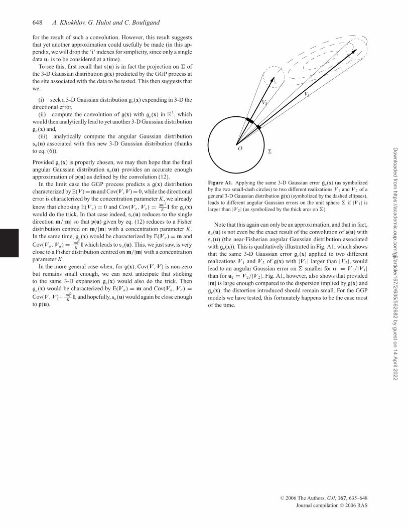
648 A. Khokhlov, G. Hulot and C. Bouligand
for the result of such a convolution. However, this result suggests
that yet another approximation could usefully be made (in this ap-
pendix, we will drop the ‘i’ indexes for simplicity, since only a single
data ui is to be considered at a time).
To see this, first recall that s(u) is in fact the projection on � of
the 3-D Gaussian distribution g(x) predicted by the GGP process at
the site associated with the data to be tested. This then suggests that
we:
(i) seek a 3-D Gaussian distribution ge(x) expending in 3-D the
directional error,
(ii) compute the convolution of g(x) with ge(x) in R3, which
would then analytically lead to yet another 3-D Gaussian distribution
ga(x) and,
(iii) analytically compute the angular Gaussian distribution
sa(u) associated with this new 3-D Gaussian distribution (thanks
to eq. (6)).
Provided ge(x) is properly chosen, we may then hope that the final
angular Gaussian distribution sa(u) provides an accurate enough
approximation of p(u) as defined by the convolution (12).
In the limit case the GGP process predicts a g(x) distribution
characterized by E(V) = m and Cov(V , V) = 0, while the directional
error is characterized by the concentration parameter K, we already
know that choosing E(V e) = 0 and Cov(V e, V e) = |m|2K I for ge(x)
would do the trick. In that case indeed, se(u) reduces to the single
direction m/|m| so that p(u) given by eq. (12) reduces to a Fisher
distribution centred on m/|m| with a concentration parameter K.
In the same time, ga(x) would be characterized by E(V a) = m and
Cov(Va, Va) = |m|2K I which leads to sa(u). This, we just saw, is very
close to a Fisher distribution centred on m/|m| with a concentration
parameter K.
In the more general case when, for g(x), Cov(V, V) is non-zero
but remains small enough, we can next anticipate that sticking
to the same 3-D expansion ge(x) would also do the trick. Then
ga(x) would be characterized by E(V a) = m and Cov(Va, Va) =Cov(V, V)+ |m|2
K I, and hopefully, sa(u) would again be close enough
to p(u).
O Σ
V1
V2
Figure A1. Applying the same 3-D Gaussian error ge(x) (as symbolized
by the two small-dash circles) to two different realizations V 1 and V 2 of a
general 3-D Gaussian distribution g(x) (symbolized by the dashed ellipses),
leads to different angular Gaussian errors on the unit sphere � if |V1| is
larger than |V2| (as symbolized by the thick arcs on �).
Note that this again can only be an approximation, and that in fact,
sa(u) is not even be the exact result of the convolution of s(u) with
se(u) (the near-Fisherian angular Gaussian distribution associated
with ge(x)). This is qualitatively illustrated in Fig. A1, which shows
that the same 3-D Gaussian error ge(x) applied to two different
realizations V 1 and V 2 of g(x) with |V1| larger than |V2|, would
lead to an angular Gaussian error on � smaller for u1 = V1/|V1|than for u2 = V2/|V2|. Fig. A1, however, also shows that provided
|m| is large enough compared to the dispersion implied by g(x) and
ge(x), the distortion introduced should remain small. For the GGP
models we have tested, this fortunately happens to be the case most
of the time.
C© 2006 The Authors, GJI, 167, 635–648
Journal compilation C© 2006 RAS
Dow
nloaded from https://academ
ic.oup.com/gji/article/167/2/635/562682 by guest on 14 April 2022
Related Documents


