Testing Planarity of Geometric Automorphisms in Linear Time

Testing Planarity of Geometric Automorphisms

in Linear Time⋆

Christoph Buchheim1 ⋆⋆ and Seok-Hee Hong2 ⋆ ⋆ ⋆

1 Universitat zu Koln, Institut fur Informatik,Pohligstraße 1, 50969 Koln, [email protected]

2 NICTA (National ICT Australia) and School of Information Technologies,University of Sydney, Australia

[email protected]

Abstract. It is a well-known result that testing a graph for planarityand, in the affirmative case, computing a planar embedding can be donein linear time. In this paper, we show that the same holds if additionallywe require that the produced drawing be symmetric with respect to agiven automorphism of the graph. This problem arises naturally in thearea of automatic graph drawing, where symmetric and planar drawingsare desired whenever possible.

Key words: graph drawing, automorphisms, symmetries, planarity

1 Introduction

Both a small number of edge crossings and the display of symmetry have beenidentified as important criteria for the readability of two-dimensional drawingsof a graph [24]. In the area of automatic graph drawing, the aim is to developnice and well-readable drawings algorithmically. This leads to the two importantproblems of minimizing the number of edge crossings and maximizing the amountof symmetry in a layout of a given graph.

In particular, planar graphs play an important role in this area. One of themost prominent results in this context is the existence of linear time algorithmsfor testing planarity of a given graph and, in the affirmative case, for computinga planar embedding [19, 2].

On the other hand, symmetric drawings of graphs are clearly preferable tonon-symmetric ones, as the complexity of the drawing for the human viewerdecreases to the same degree as the symmetric structure in the drawing increases.Furthermore, symmetric drawings are regarded as more beautiful in general. The

⋆

An extended abstract of this paper has been published in the proceedings of ISAAC 2002 [3].⋆⋆

The first author is supported by the Marie Curie Research Training Network ADONET 504438

funded by the EU. This paper was partially written when he was visiting the University of Sydney.⋆ ⋆ ⋆

The second author was supported by a grant from the Australian Research Council. National ICT

Australia is funded by the Australian Government’s Backing Australia’s Ability initiative, in part

through the Australian Research Council.

problem of detecting symmetries in a given graph can be solved in linear timefor planar graphs [15–18]. In general, the problem is NP-hard [22]. Nevertheless,exact approaches for general graphs have been devised, using branch-and-cut [5]or group-theoretic methods [1]. Moreover, several heuristic approaches to theproblem have been proposed [20, 13, 7]. It was also shown that the well-knownspring embedder method has a tendency to display symmetry [11]. An importantrelaxation of the symmetry detection problem is to consider nearly symmetricdrawings [8, 9, 6].

In the following, we assume throughout that a geometric automorphism π ofsome graph G is given, i.e., an automorphism of G that can be visualized by sometwo-dimensional drawing of G [11]. In general, there are many different drawingsrealizing π in this case; see Figs. 1(a) and 1(b) as an example. In particular, thenumber of edge crossings will vary for different visualizations of π.

In a former paper [4], we discussed the problem of minimizing the number ofcrossings over all possible drawings of G visualizing π; an extended abstract waspublished in [3]. With respect to this criterion, the drawing in Fig. 1(b) wouldbe preferable to the one in Fig. 1(a), as it has less crossings. We showed thatthis problem is NP-hard, even if strongly restricted in several variations.

In the present paper, we focus on the planarity problem: given a geometricautomorphism π of a graph G, is there a planar drawing of G visualizing π? Weshow that this problem can be solved in linear time. In the case of a positiveanswer, we can also construct such a drawing in linear time. See Fig. 2 forexamples of drawings displaying planar symmetries.

0

1

2

3

4

5

6

7

8

9

10

11

12

13

14

15

16

17

18

19

20

21

22

23

(a)

0

1

2

3

4

5

67

8

9

10

11

1213

14 15

16

17

18

19

20

21

22

23

(b)

0

12

3

4

5

6

7

8

9

10

11

12

13

14

1516

17

1819

20

21

22

23

(c)

Fig. 1. Three drawings displaying the same graph. The graph is planar, as shown bythe drawing (c), but the rotational automorphism displayed in (a) and (b) cannot bedisplayed by any planar drawing

Our result generalizes the corresponding result for testing planarity of graphs.The algorithm is built up in a way similar to the algorithms for finding a planarautomorphism group of maximum size presented in [15–18], which is based on

2

0

1

2

3

4

5

6

7

8 9

1011

12 13

1415

(a)

0

1

2 3

4 5

6

7 8

9

10

11

12

(b)

0

1

2

4 5

6 78 9

10 11

(c)

Fig. 2. Three drawings displaying planar automorphisms of different graphs. In (a),all displayed automorphisms are rotations of order four, while (b) displays rotations oforder three and reflections. Drawing (c) displays only reflectional automorphisms

the connectivity of the graph: the case of a triconnected graph is settled first,then SPQR-trees are used to reduce the biconnected case to the triconnectedone, then the block-cutvertex-tree is used to reduce the oneconnected case tothe biconnected one, and finally the disconnected case is solved.

The remainder of this paper is organized as follows: in Section 2, we introducethe necessary definitions and give a more formal statement of the problems weconsider. In Section 3, we recall the SPQR-tree datastructure and examine theconnection between automorphisms of a graph and its SPQR-tree. The main partis Section 4, where we show how to test planarity of geometric automorphismsin linear time. Section 5 concludes. In Appendix A, we illustrate our algorithmby an example.

2 Preliminaries

Throughout this paper, we consider a simple graph G = (V, E) with n verticesand m edges. A drawing of a graph is a representation of its vertices by distinctpoints of the plane and of its edges by arbitrary curves in the plane that connectthe corresponding points but do not intersect any other vertex point. A drawingof G is plane if no two curves representing edges of G intersect, i.e., have acommon point except for possibly at a vertex point. A graph is said to be planarif it admits any plane drawing.

An automorphism of G is a permutation π : V → V of its vertices such thattwo vertices v and w are adjacent if and only if π(v) and π(w) are. The orderof an automorphism π is the smallest positive integer k such that πk is theidentity. An induced subgraph G′ = (V ′, E′) of G is fixed by π if π(V ′) = V ′.In particular, a vertex v is fixed if π(v) = v, and an edge (v, w) is fixed if theset {v, w} is fixed, i.e, if v and w are either both fixed or exchanged by π. If G′ isa fixed subgraph, then the restriction π|G′ of π to G′, defined by π|G′(v) = π(v)for all v ∈ V ′, is an automorphism of G′. The orbit of a subgraph G′ = (V ′, E′)

3

1

2

34

5

1

2

3 4

5

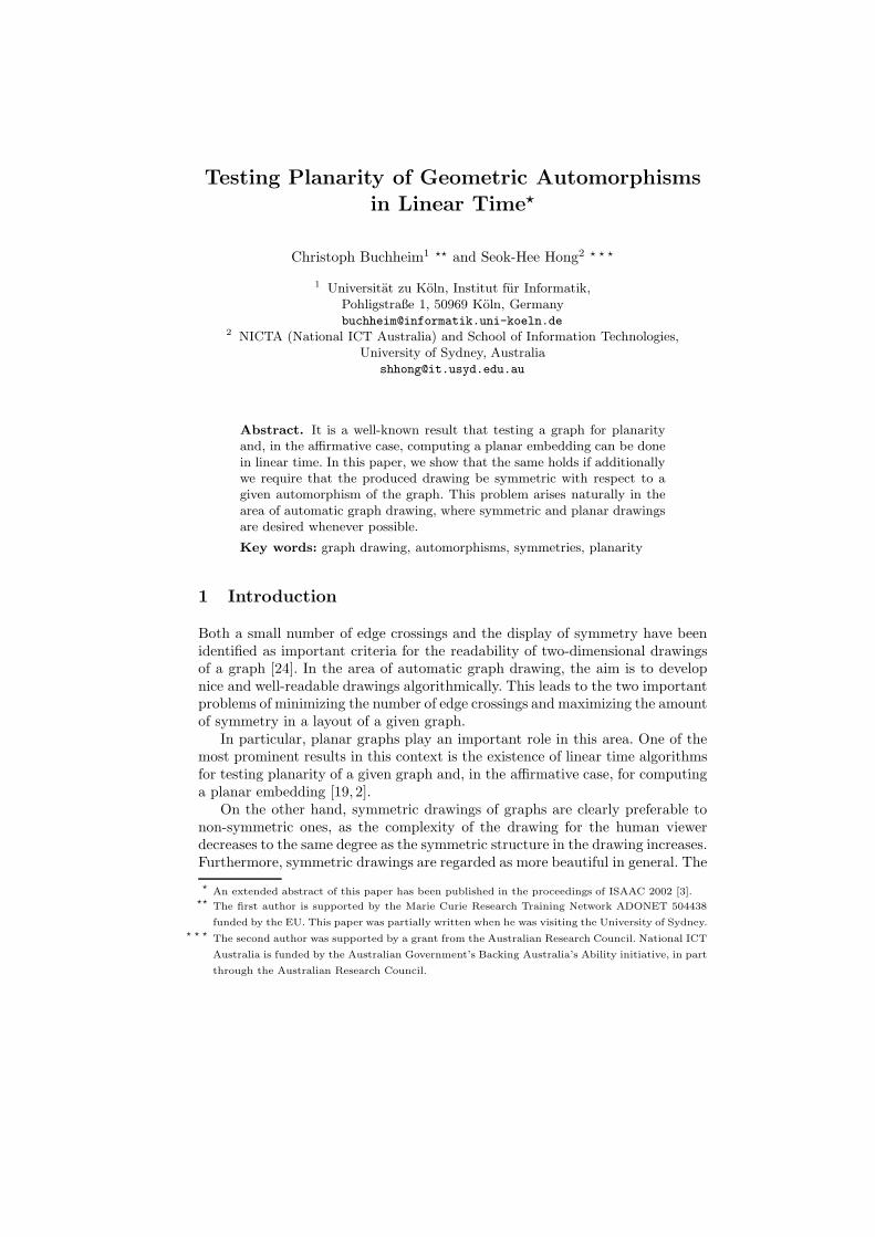
Fig. 3. Drawings of the rotation π = (12345) having exponents one and three

of G under π is the graph with vertex set {πk(v) | v ∈ V ′, k integer} and edgeset {(πk(v), πk(w)) | (v, w) ∈ E′, k integer}. This in particular defines the orbitof a single vertex or a single edge.

A drawing of G is called reflectionally symmetric if it is fixed by some non-trivial reflection of the plane in an axis, the reflection axis . Analogously, arotationally symmetric drawing of G is a drawing of G fixed by some non-trivialrotation of the plane around a center point, the rotation center. A drawing iscalled symmetric if it is fixed by any isometry of the plane, or, equivalently, if itis either reflectionally or rotationally symmetric [11].

A geometric automorphism of G is an automorphism induced by a symmetricdrawing of G [11]. A reflection (rotation) of G is an automorphism of G inducedby a reflectionally (rotationally) symmetric drawing of G.

For a given symmetric drawing D inducing a rotation π of order k, there isexactly one e ∈ {1, . . . , k} such that rotating D by 360/k degrees in clockwiseorder around the rotation center maps each vertex v to πe(v). The number e isthe exponent of the drawing D; see Fig. 3.

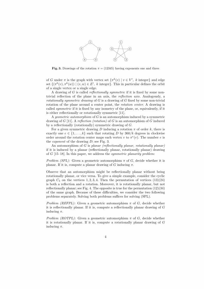
An automorphism of G is planar (reflectionally planar, rotationally planar)if it is induced by a planar (reflectionally planar, rotationally planar) drawingof G [15–18]. In this paper, we address the symmetric planarity problem:

Problem (SPL): Given a geometric automorphism π of G, decide whether it isplanar. If it is, compute a planar drawing of G inducing π.

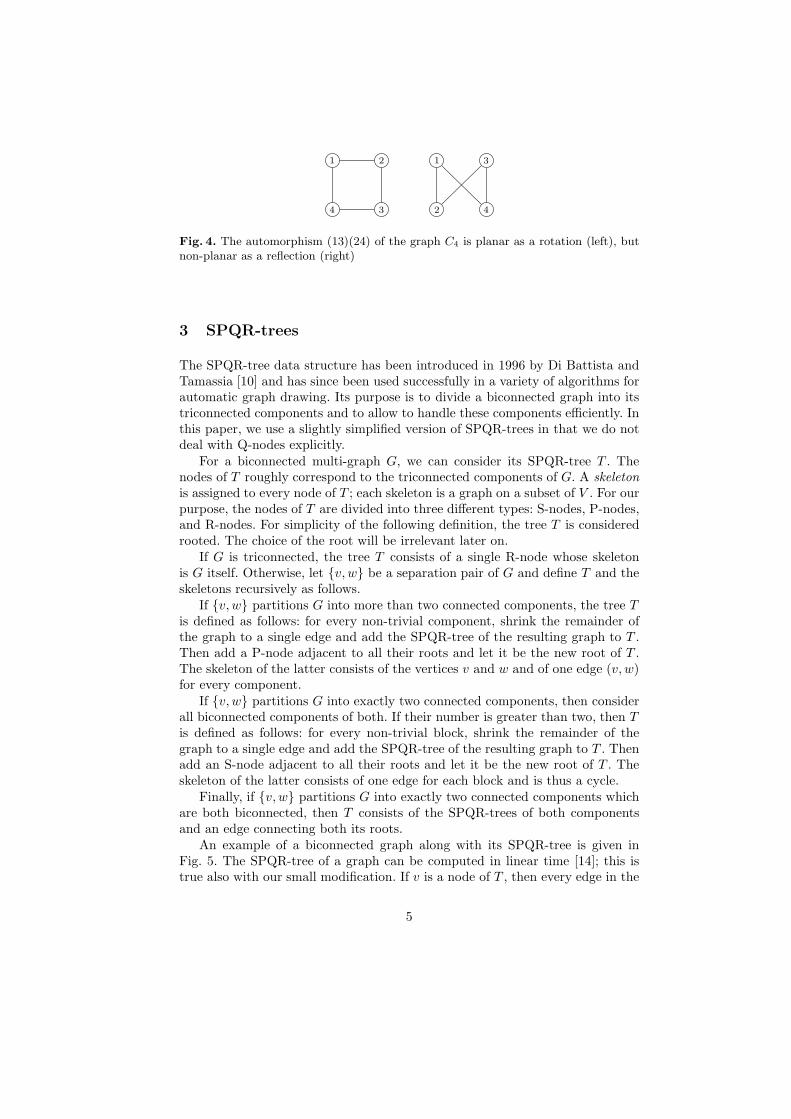
Observe that an automorphism might be reflectionally planar without beingrotationally planar, or vice versa. To give a simple example, consider the cyclicgraph C4 on the vertices 1, 2, 3, 4. Then the permutation of vertices (13)(24)is both a reflection and a rotation. Moreover, it is rotationally planar, but notreflectionally planar; see Fig. 4. The opposite is true for the permutation (12)(34)of the same graph. Because of these difficulties, we consider the two followingproblems separately. Solving both problems suffices for solving (SPL).

Problem (REFPL): Given a geometric automorphism π of G, decide whetherit is reflectionally planar. If it is, compute a reflectionally planar drawing of Ginducing π.

Problem (ROTPL): Given a geometric automorphism π of G, decide whetherit is rotationally planar. If it is, compute a rotationally planar drawing of Ginducing π.

4

1 2

34

1

2

3

4

Fig. 4. The automorphism (13)(24) of the graph C4 is planar as a rotation (left), butnon-planar as a reflection (right)

3 SPQR-trees

The SPQR-tree data structure has been introduced in 1996 by Di Battista andTamassia [10] and has since been used successfully in a variety of algorithms forautomatic graph drawing. Its purpose is to divide a biconnected graph into itstriconnected components and to allow to handle these components efficiently. Inthis paper, we use a slightly simplified version of SPQR-trees in that we do notdeal with Q-nodes explicitly.

For a biconnected multi-graph G, we can consider its SPQR-tree T . Thenodes of T roughly correspond to the triconnected components of G. A skeletonis assigned to every node of T ; each skeleton is a graph on a subset of V . For ourpurpose, the nodes of T are divided into three different types: S-nodes, P-nodes,and R-nodes. For simplicity of the following definition, the tree T is consideredrooted. The choice of the root will be irrelevant later on.

If G is triconnected, the tree T consists of a single R-node whose skeletonis G itself. Otherwise, let {v, w} be a separation pair of G and define T and theskeletons recursively as follows.

If {v, w} partitions G into more than two connected components, the tree Tis defined as follows: for every non-trivial component, shrink the remainder ofthe graph to a single edge and add the SPQR-tree of the resulting graph to T .Then add a P-node adjacent to all their roots and let it be the new root of T .The skeleton of the latter consists of the vertices v and w and of one edge (v, w)for every component.

If {v, w} partitions G into exactly two connected components, then considerall biconnected components of both. If their number is greater than two, then Tis defined as follows: for every non-trivial block, shrink the remainder of thegraph to a single edge and add the SPQR-tree of the resulting graph to T . Thenadd an S-node adjacent to all their roots and let it be the new root of T . Theskeleton of the latter consists of one edge for each block and is thus a cycle.

Finally, if {v, w} partitions G into exactly two connected components whichare both biconnected, then T consists of the SPQR-trees of both componentsand an edge connecting both its roots.

An example of a biconnected graph along with its SPQR-tree is given inFig. 5. The SPQR-tree of a graph can be computed in linear time [14]; this istrue also with our small modification. If v is a node of T , then every edge in the

5

skeleton of v either corresponds to an edge of G or to a neighboring node w of vin T . In the latter case, the edge is called virtual and it is said that this virtualedge represents the skeleton of w. Two nodes in T are adjacent if and only ifthe skeleton of each node contains an edge representing the other’s. In Fig. 5,virtual edges are represented by dotted lines.

0

2

5

7

812

13

15

16

18

19

25

(a)

8 15

8 15

16

0 18

158

19

19 15

5

8 19

138 15

12

2

2

12

7 25

(b)

S

S

SP

R

R

R

(c)

Fig. 5. A biconnected graph (a) and its SPQR-tree (c); the skeletons are shown in (b)

Coming back to symmetries, observe that any automorphism π of G inducesan automorphism πT of T . If some node of T is fixed by πT , we further get aninduced automorphism on the skeleton ν corresponding to that node, which wewill simply call the restriction of π to ν, denoted by π|ν . It is easy to see—and willbe used in the following—that the restriction of a geometric automorphism to anyfixed skeleton is a geometric automorphism of the same type again, i.e., remainsa rotation or reflection. Furthermore, the restriction of a planar automorphismto a skeleton remains planar.

Lemma 1. For every automorphism π of G, the nodes of T with skeletons fixedby π induce a subtree of T .

Proof. Consider the induced automorphism πT of T . If there was a path P in Tconnecting two fixed nodes but containing non-fixed nodes, then the nodes in Pand πT (P ) would induce a subgraph of T containing a cycle. ⊓⊔

Lemma 2. Let π be any automorphism of G. Then either there is a skeletonof T fixed by π or there is a separation pair of G fixed by π.

Proof. Consider the center of T , i.e., the set C of nodes maximizing the minimaldistance to any leaf of T . If C contains a single node, this node must be fixed byall automorphisms of T , in particular by πT . The corresponding skeleton is thusfixed by π. Otherwise C contains two adjacent nodes. In this case, the connectingedge is fixed by πT , i.e., the corresponding separation pair of G is fixed by π. ⊓⊔

6

4 Testing Planarity

In this section, we show that the problem (SPL) can be solved in linear time.First observe that planarity does not depend on whether we restrict ourselves tostraight-line drawings or not. This follows from

Theorem 1 (Mani [21]). Every triconnected planar graph can be drawn as theskeleton of a polytope in the three-dimensional Euclidean space such that everyautomorphism of the graph is induced by an isometry of the polytope.

Theorem 2. For every planar drawing of an automorphism π, there exists aplanar drawing of π with straight-line edges that induces the same embedding ofthe underlying graph.

Proof. Consider a planar drawing of G inducing the automorphism π and let Fbe its outer face, which is necessarily fixed by π. First assume that G is tricon-nected. Choose a polytope P as in Mani’s Theorem. Then F corresponds to afacet of P fixed by π, so that an appropriate projection of P to the plane yieldsa planar straight-line drawing of π with F as its outer face. As G is triconnected,the induced embedding is the same as the original one.

If G is not triconnected, we claim that there is a triconnected graph G′ with aplanar automorphism π′ such that G is a fixed subgraph of G′ and π′|G = π; theresult for π′ then implies the one for π. In fact, if G is biconnected, the graph G′

can be obtained by the star triangulation [18], which adds a new vertex intoeach face of G that is adjacent to each vertex of the face. If G is one-connectedor disconnected, it is easy to make it biconnected without losing symmetry. ⊓⊔

It is a well-known result by Fary [12] that every planar graph admits a planarstraight-line drawing. Theorem 2 shows that this still holds under the additionalrequirement that a given automorphism be displayed.

In the following, we will prove our main result. The outline of our algorithm tosolve problem (SPL) is similar to the one of the planar automorphism detectionalgorithm presented in [15–18]. In particular, we also consider the triconnected,biconnected, one-connected, and disconnected cases one after another. We splitup the proof according to these cases. Notice however that our result does notfollow from the results in [15–18], as the presented detection algorithm cannotbe forced to detect the given specific automorphism π. Furthermore, the factthat in our problem we deal with a single automorphism allows a very clear andnatural construction of the desired planar drawing, if one exists.

The general idea of our proof is the following: for triconnected graphs, theresult follows from Mani’s Theorem. For a k-connected graph with k = 0, 1, 2, weconsider its (k + 1)-connected components and distinguish those being fixed bythe given automorphism from those not being fixed. On the fixed components,a geometric automorphism of G induces a geometric automorphism of the sametype, so we can apply the (k+1)-connected case. The non-fixed components canbe divided into orbits with respect to the given automorphism; components inthe same orbit are isomorphic. For every orbit, we can pick one component, draw

7

it using an arbitrary planar drawing algorithm, and draw the other componentsin the same orbit by copying this drawing along the isometry corresponding tothe given automorphism. The only tricky question is how to glue together allsingle component drawings preserving planarity.

In the first step of our algorithm, we check the graph G for planarity, whichcan be done in linear time [19, 2]. In the case of a negative result, we know that πis neither reflectionally planar nor rotationally planar, so in the following we mayalways assume that G is planar and hence m ∈ O(n).

Lemma 3. The problems (REFPL) and (ROTPL) can be solved in O(n) timefor triconnected graphs.

Proof. We first check whether there is a face F in the unique combinatorialembedding of G that is fixed by π such that π|F is reflectionally (rotationally)planar. As F is a cycle, this can easily be done in linear time. If the answer isnegative, we can state that π is not reflectionally (rotationally) planar. Indeed,the outer face in any reflectionally (rotationally) planar drawing of π must befixed by π and the restriction of π to the outer face is surely reflectionally(rotationally) planar; compare Lemma 1 in [18].

Otherwise, if such a face F exists, we can use the same projection as in theproof of Theorem 2 to show that the unique topological embedding of G withouter face F can be realized by a reflectionally (rotationally) planar drawingof π. A linear time algorithm for computing a nice drawing is devised in [18]. ⊓⊔

Lemma 4. The problems (REFPL) and (ROTPL) can be solved in O(n) timefor biconnected graphs.

Proof. Consider the SPQR-tree T of G. First determine for every node of Twhether its skeleton is fixed by π or not. For every fixed skeleton ν, we nextcheck whether π|ν is reflectionally (rotationally) planar. For R-nodes, we canuse Lemma 3, as the skeleton of an R-node is triconnected. For S-nodes andP-nodes, this is trivial: the skeleton of an S-node is a cycle, so that reflectional(rotational) planarity of π|ν can be checked easily in this case; see Fig. 6. Theskeleton of a P-node is a bunch of parallel edges, so that π|ν in this case isreflectionally planar if and only if either the two vertices are exchanged or atmost one of the edges is fixed and the remaining edges are divided into orbits ofsize two. It is rotationally planar if and only if the two vertices are exchangedand at most one of the edges is fixed and the remaining edges are divided intoorbits of size two; see Fig. 7.

In the event of any negative answer, i.e., if there is any fixed skeleton ν suchthat π|ν is not reflectionally (rotationally) planar, we can state that π is notreflectionally (rotationally) planar. Otherwise, we claim that π is reflectionally(rotationally) planar and construct a reflectionally (rotationally) planar drawinginducing π as follows.

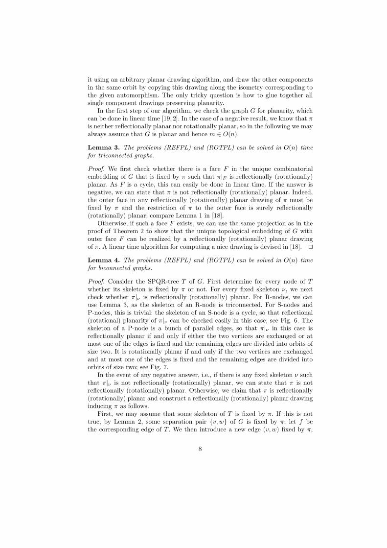
First, we may assume that some skeleton of T is fixed by π. If this is nottrue, by Lemma 2, some separation pair {v, w} of G is fixed by π; let f bethe corresponding edge of T . We then introduce a new edge (v, w) fixed by π,

8

Fig. 6. The skeleton of an S-node drawn reflectionally planar (left and middle) androtationally planar (right); fixed edges are drawn boldly

Fig. 7. The skeleton of a P-node drawn reflectionally planar (left and middle) androtationally planar (right); fixed edges are drawn boldly

which can be removed in the final drawing. In other words, we split up f byintroducing a new P-node that is fixed by π; see Fig. 8.

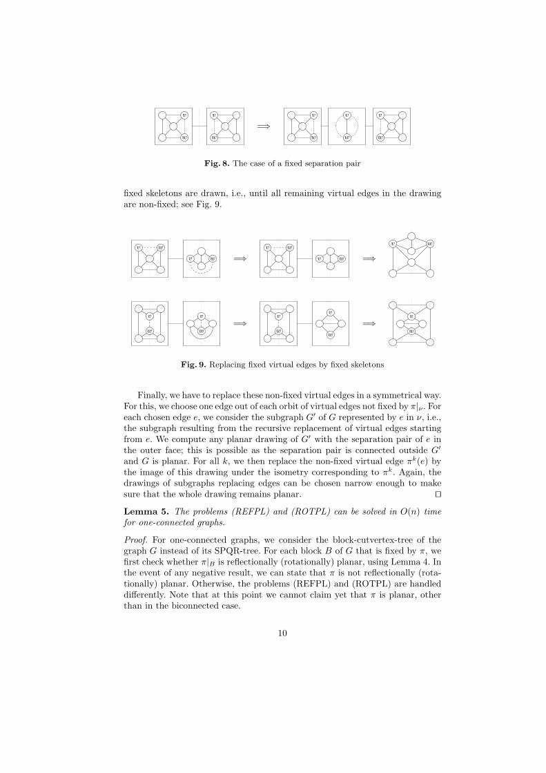
Now choose any fixed skeleton ν and compute any reflectionally (rotationally)planar drawing of the geometric automorphism π|ν , using Lemma 3 for R-nodesand trivial algorithms for P-nodes and S-nodes. If there is any other skeletonfixed by π, then by Lemma 1 there is a fixed skeleton neighboring ν in T , so thatone of the virtual edges e of ν must be fixed by π|ν ; either e is reversed by π|νor both end vertices of e are fixed. Let e represent the skeleton ν′ and let {v, w}be the corresponding separation pair. We can now replace the drawing of e by areflectionally (rotationally) planar drawing of π|ν′ whose outer face contains theseparation pair {v, w}.

More precisely, we compute a planar drawing of π|ν′ and remove the virtualedge (v, w) corresponding to ν in this drawing. The vertices v and w then sharea face F in this drawing of π|ν′ . As F contained the fixed edge (v, w) before, itmust be fixed by π|ν′ . We may assume that F is the outer face of the computedplanar drawing of π|ν′ ; otherwise we can obtain this situation by applying thetransformation (x, y) 7→ (x/(x2 + y2), y/(x2 + y2)) to the drawing of π|ν′ , wherewe assume that the former center point of (v, w) is the origin of R2. Noticethat this transformation is not linear, but it is injective on R2 \ {0}, so that thetransformed drawing is planar again. Furthermore, the property of the drawingbeing rotationally (reflectionally) symmetric is preserved.

Replacing the virtual edge e in the drawing of π|ν by the so constructeddrawing of π|ν′ now yields a planar drawing of π|ν∪ν′ . The two drawings fittogether as the skeletons ν and ν′ share the vertices v and w. Obviously, thedrawings replacing edges can be made narrow enough to make sure that thewhole drawing remains planar. We iterate this replacement process until all

9

vv

ww

=⇒

vvv

www

Fig. 8. The case of a fixed separation pair

fixed skeletons are drawn, i.e., until all remaining virtual edges in the drawingare non-fixed; see Fig. 9.

v

v

w

w

=⇒ v

v

w

w

=⇒

v w

vv

ww

=⇒

vv

ww

=⇒v

w

Fig. 9. Replacing fixed virtual edges by fixed skeletons

Finally, we have to replace these non-fixed virtual edges in a symmetrical way.For this, we choose one edge out of each orbit of virtual edges not fixed by π|ν . Foreach chosen edge e, we consider the subgraph G′ of G represented by e in ν, i.e.,the subgraph resulting from the recursive replacement of virtual edges startingfrom e. We compute any planar drawing of G′ with the separation pair of e inthe outer face; this is possible as the separation pair is connected outside G′

and G is planar. For all k, we then replace the non-fixed virtual edge πk(e) bythe image of this drawing under the isometry corresponding to πk. Again, thedrawings of subgraphs replacing edges can be chosen narrow enough to makesure that the whole drawing remains planar. ⊓⊔

Lemma 5. The problems (REFPL) and (ROTPL) can be solved in O(n) timefor one-connected graphs.

Proof. For one-connected graphs, we consider the block-cutvertex-tree of thegraph G instead of its SPQR-tree. For each block B of G that is fixed by π, wefirst check whether π|B is reflectionally (rotationally) planar, using Lemma 4. Inthe event of any negative result, we can state that π is not reflectionally (rota-tionally) planar. Otherwise, the problems (REFPL) and (ROTPL) are handleddifferently. Note that at this point we cannot claim yet that π is planar, otherthan in the biconnected case.

10

We start with the easier problem (ROTPL), where we first check whetherthe number of fixed blocks is greater than one. If so, we can state that π is notrotationally planar; see Theorem 9 in [17]. Otherwise, we can show that π isrotationally planar by constructing a drawing as follows.

If there is exactly one fixed block B, we can compute a rotationally planardrawing of π|B by Lemma 4. Then we can add the remaining non-fixed blockssymmetrically, one orbit after another. For every such block B′ containing a cutvertex c already drawn, we first compute any planar drawing of B′ with c onits outer face. Then, for all k, we attach the image of this drawing under theisometry corresponding to πk to the cut vertex πk(c), thus adding a drawingof πk(B′). Obviously, this can be done without creating any edge crossings; seeFig. 10(a) for an illustration. Notice that c might be fixed by π, in this case allvertices πk(c) are identical.

Next, assume that no block of G is fixed by π. Then some cut vertex c of Gmust be fixed by π. Now the subgraphs of G connected by c can be divided intoorbits, drawn in an arbitrary planar way with c on the outer face, and placedaround c in a similar way as in the case of a fixed block; see Fig 10(b).

(a) (b)

Fig. 10. Reduction to biconnected graphs in the rotation case; fixed blocks are shaded

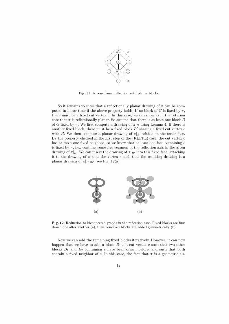
Now consider the problem (REFPL). We claim that π is reflectionally planarif and only if for every fixed block B the restriction π|B is reflectionally planarand for every fixed cut vertex c in B, either c has at most one fixed neighborin B or c belongs to at most one fixed block (namely B). Using Lemma 4, thisproperty can be checked in linear time.

It is easy to see that π cannot be reflectionally planar otherwise, i.e., if therestriction to some fixed block is not reflectionally planar or if there are twofixed blocks B1 and B2 sharing a cut vertex c such that in B1 the vertex c hastwo fixed neighbors v1 and v2. In the second case, the vertex c would have tolie between v1 and v2 on the reflection axis in any drawing of π. It is easy tosee that any drawing of π|B2

would have to cross either one of the edges (c, v1)and (c, v2) or a path connecting v1 and v2 in B1 not using c, which exists as B1

is biconnected; see Fig. 11 for an example.

11

c

v1

v2 B1

B2

Fig. 11. A non-planar reflection with planar blocks

So it remains to show that a reflectionally planar drawing of π can be com-puted in linear time if the above property holds. If no block of G is fixed by π,there must be a fixed cut vertex c. In this case, we can show as in the rotationcase that π is reflectionally planar. So assume that there is at least one block Bof G fixed by π. We first compute a drawing of π|B using Lemma 4. If there isanother fixed block, there must be a fixed block B′ sharing a fixed cut vertex cwith B. We then compute a planar drawing of π|B′ with c on the outer face.By the property checked in the first step of the (REFPL) case, the cut vertex chas at most one fixed neighbor, so we know that at least one face containing cis fixed by π, i.e., contains some free segment of the reflection axis in the givendrawing of π|B . We can insert the drawing of π|B′ into this fixed face, attachingit to the drawing of π|B at the vertex c such that the resulting drawing is aplanar drawing of π|B∪B′ ; see Fig. 12(a).

(a) (b)

Fig. 12. Reduction to biconnected graphs in the reflection case. Fixed blocks are firstdrawn one after another (a), then non-fixed blocks are added symmetrically (b)

Now we can add the remaining fixed blocks iteratively. However, it can nowhappen that we have to add a block B at a cut vertex c such that two otherblocks B1 and B2 containing c have been drawn before, and such that bothcontain a fixed neighbor of c. In this case, the fact that π is a geometric au-

12

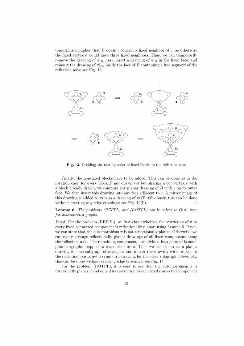
tomorphism implies that B doesn’t contain a fixed neighbor of c, as otherwisethe fixed vertex c would have three fixed neighbors. Thus, we can temporarilyremove the drawing of π|B1

, say, insert a drawing of π|B in the freed face, andreinsert the drawing of π|B1

inside the face of B containing a free segment of thereflection axis; see Fig. 13.

c c

BB1

B2

=⇒c cc

BB1

B2

=⇒c c

BB1

B2

=⇒c

B

B1

B2

Fig. 13. Deciding the nesting order of fixed blocks in the reflection case

Finally, the non-fixed blocks have to be added. This can be done as in therotation case: for every block B not drawn yet but sharing a cut vertex c witha block already drawn, we compute any planar drawing of B with c on its outerface. We then insert this drawing into any face adjacent to c. A mirror image ofthis drawing is added to π(c) as a drawing of π(B). Obviously, this can be donewithout creating any edge crossings; see Fig. 12(b). ⊓⊔

Lemma 6. The problems (REFPL) and (ROTPL) can be solved in O(n) timefor disconnected graphs.

Proof. For the problem (REFPL), we first check whether the restriction of π toevery fixed connected component is reflectionally planar, using Lemma 5. If not,we can state that the automorphism π is not reflectionally planar. Otherwise, wecan easily arrange reflectionally planar drawings of all fixed components alongthe reflection axis. The remaining components are divided into pairs of isomor-phic subgraphs mapped to each other by π. Thus we can construct a planardrawing for one subgraph of each pair and mirror the drawing with respect tothe reflection axis to get a symmetric drawing for the other subgraph. Obviously,this can be done without creating edge crossings; see Fig. 14.

For the problem (ROTPL), it is easy to see that the automorphism π isrotationally planar if and only if its restriction to each fixed connected component

13

Fig. 14. Reduction to connected graphs in the reflection case

is rotationally planar with the same exponent e, and a drawing of π can easilybe constructed by drawing the fixed components around each other; see Fig. 15.Note that only one connected component of the graph can contain a fixed vertexif π is a rotation.

Fig. 15. Reduction to connected graphs in the rotation case

It remains to explain how to find a common exponent for all fixed componentsor to state that there is none. Fig. 16 shows that this is crucial in the rotationcase. So let G′ be any fixed component of G. We claim that either there existsan integer e such that any planar drawing of π|G′ has exponent e or −e, or thereis a planar drawing of π|G′ for any exponent; moreover, for every component,all possible exponents can be determined in linear time. Then it is easy to checkwhether there is a common exponent for all fixed components, and if there isone, to construct a drawing with this exponent for the whole graph.

To prove our claim, first assume that G′ has a cut vertex fixed by π|G′ . Thenthe exponent is arbitrary. A drawing with a given exponent can be producedby permuting the components of G′ resulting from deleting c, according to thisexponent. Otherwise, if G′ does not contain a fixed cut vertex, it remains con-nected after removing any fixed vertex—as π is a rotation, there can be at mostone fixed vertex. Let v be any non-fixed vertex of G′. Choose any path from vto π|G′(v) without fixed vertices and determine e such that (π|G′)e(v) is the firstvertex after v on this path that belongs to the orbit of v. Such e exists, as π|G′(v)belongs to the path. Then e and −e are the only possible exponents of a planardrawing of π|G′ , as otherwise any path from v to (π|G′)e(v) would have to crossits own image under π. ⊓⊔

14

Fig. 16. A non-planar rotation with planar components

We can now conclude the proof of

Theorem 3. Problem (SPL) can be solved in O(n) time.

Proof. The automorphism π is planar if and only if it is induced by a reflec-tionally or a rotationally symmetric planar drawing of G [11]. Hence the resultfollows from Lemmas 3 to 6. ⊓⊔

5 Conclusion

We showed that planarity of geometric automorphisms can be tested in lineartime and that planar drawings can be computed in linear time whenever theyexist. This is true in spite of the fact that the crossing minimization problemfor geometric automorphisms is very hard [4]. However, as in the case of graphswithout fixed automorphisms, one can use the presented algorithm for a heuristicapproach to the crossing minimization problem via the computation of maximalplanar symmetric subgraphs of G with respect to π: starting with an emptygraph H and traversing all edge orbits of π, one can check in linear time whetheradding the current edge orbit to H would destroy planarity of π|H or not. Inthe former case, the edge orbit is discarded, while in the latter case it is addedpermanently to H . It is clear that the resulting geometric automorphism π|H ismaximally planar.

Finally, we would like to mention that our algorithm, as presented, can onlycheck single geometric automorphisms for planarity. However, the group of allautomorphisms displayed by a specific drawing of the graph cannot always begenerated by a single automorphism. More precisely, it can be a dihedral group,jointly generated by a rotational and a reflectional symmetry [11]. It wouldthus be desirable to have an algorithm checking simultaneous planarity of twogeometric automorphisms, i.e., checking whether there is a planar drawing of thegraph displaying both. We are convinced that the algorithm presented in thispaper can be extended to this case.

References

1. D. Abelson, S. Hong, and D. Taylor. A group-theoretic method for drawing graphssymmetrically. In S. G. Kobourov and M. T. Goodrich, editors, Graph Drawing

2002, volume 2528 of LNCS, pages 86–97. Springer-Verlag, 2002.

15

2. K. Booth and G. Lueker. Testing for the consecutive ones property, interval graphsand graph planarity using PQ-tree algorithms. Journal of Computer and System

Sciences, 13:335–379, 1976.3. C. Buchheim and S. Hong. Crossing minimization for symmetries. In P. Bose and

P. Morin, editors, ISAAC 2002, volume 2518 of LNCS, pages 563–574. Springer-Verlag, 2002.

4. C. Buchheim and S. Hong. Crossing minimization for symmetries. Theory of

Computing Systems, 38(3):293–311, 2005.5. C. Buchheim and M. Junger. Detecting symmetries by branch & cut. In P. Mutzel,

M. Junger, and S. Leipert, editors, Graph Drawing 2001, volume 2265 of LNCS,pages 178–188. Springer-Verlag, 2001.

6. C. Buchheim and M. Junger. An integer programming approach to fuzzy symmetrydetection. In G. Liotta, editor, Graph Drawing 2003, volume 2912 of LNCS, pages166–177. Springer-Verlag, 2004.

7. H. Carr and W. Kocay. An algorithm for drawing a graph symmetrically. Bulletin

of the ICA, 27:19–25, 1999.8. H. Chen, H. Lu, and H. Yen. On maximum symmetric subgraphs. In J. Marks, ed-

itor, Graph Drawing 2000, volume 1984 of LNCS, pages 372–383. Springer-Verlag,2001.

9. M. Chuang and H. Yen. On nearly symmetric drawings of graphs. In IV 2002,pages 489–494, 2002.

10. G. Di Battista and R. Tamassia. On-line planarity testing. SIAM Journal on

Computing, 25(5):956–997, 1996.11. P. Eades and X. Lin. Spring algorithms and symmetry. Theoretical Computer

Science, 240(2):379–405, 2000.12. I. Fary. On straight lines representations of planar graphs. Acta Scientiarum

Mathematicarum, 11:229–233, 1948.13. H. de Fraysseix. An heuristic for graph symmetry detection. In J. Kratochvıl, ed-

itor, Graph Drawing 1999, volume 1731 of LNCS, pages 276–285. Springer-Verlag,1999.

14. C. Gutwenger and P. Mutzel. A linear time implementation of SPQR trees.In J. Marks, editor, Graph Drawing 2000, volume 1984 of LNCS, pages 77–90.Springer-Verlag, 2001.

15. S. Hong and P. Eades. Symmetric layout of disconnected graphs. In T. Ibaraki,N. Katoh, and H. Ono, editors, ISAAC 2003, volume 2906 of LNCS, pages 405–414.Springer-Verlag, 2003.

16. S. Hong and P. Eades. Drawing planar graphs symmetrically, II: Biconnectedplanar graphs. Algorithmica, 42(2):159–197, 2005.

17. S. Hong and P. Eades. Drawing planar graphs symmetrically, III: Oneconnectedplanar graphs. Algorithmica, 44(1):67–100, 2006.

18. S. Hong, B. McKay, and P. Eades. Symmetric drawings of triconnected planargraphs. In SODA 2002, pages 356–365, 2002.

19. J. Hopcroft and R. Tarjan. Efficient planarity testing. Journal of the Association

for Computing Machinery, 21:549–568, 1974.20. R. J. Lipton, S. C. North, and J. S. Sandberg. A method for drawing graphs. In

ACM Symposium on Computational Geometry, pages 153–160, 1985.21. P. Mani. Automorphismen von polyedrischen Graphen. Mathematische Annalen,

192:279–303, 1971.22. J. Manning. Computational complexity of geometric symmetry detection in graphs.

In Great Lakes Computer Science Conference, volume 507 of LNCS, pages 1–7.Springer-Verlag, 1989.

16

23. J. Manning and M. J. Atallah. Fast detection and display of symmetry in outer-planar graphs. Discrete Applied Mathematics, 39(1):13–35, 1992.

24. H. Purchase. Which aesthetic has the greatest effect on human understanding? InG. Di Battista, editor, Graph Drawing ’97, volume 1353 of LNCS, pages 248–261.Springer-Verlag, 1997.

17

A An Example

In this appendix, we illustrate the construction of a planar drawing in the reflec-tionally symmetric case by an example. The graph G is displayed in Fig. 17. Thegiven automorphism π is marked by the dashed arrows showing which verticesof G are mapped to each other by π, all other vertices are fixed.

0

1

2

3

4

5

67

8

10

11

12

13

14

15

16

17

18

19

20

21

22

23

24

25

9

Fig. 17. The graph G and the automorphism π. Vertices belonging to a fixed connectedcomponent are shaded; two components are fixed, two are not

As G is disconnected, the first step of the algorithm consists of determiningthe connected components of G and dividing them into fixed components andpairs of non-fixed components being mapped to each other by π.

We first draw the large fixed component G′ of G shown in Fig. 18. For this,we have to compute its block-cutvertex-tree. The cut vertices are marked inFig. 18.

0

1

2

3

4

5

7

8

10

12

13

14

15

16

17

18

19

20

25

Fig. 18. The connected component G′ with cut vertices shaded

18

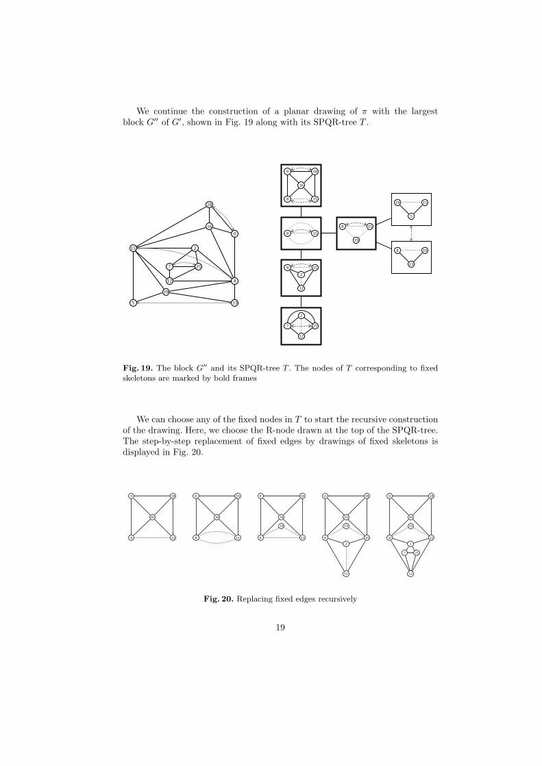
We continue the construction of a planar drawing of π with the largestblock G′′ of G′, shown in Fig. 19 along with its SPQR-tree T .

0

2

5

7

812

13

15

16

18

19

25

8 15

8 15

16

0 18

158

19

19 15

5

8 19

138 15

12

2

2

12

7 25

Fig. 19. The block G′′ and its SPQR-tree T . The nodes of T corresponding to fixed

skeletons are marked by bold frames

We can choose any of the fixed nodes in T to start the recursive constructionof the drawing. Here, we choose the R-node drawn at the top of the SPQR-tree.The step-by-step replacement of fixed edges by drawings of fixed skeletons isdisplayed in Fig. 20.

8 15

16

0 18

12

8 15

16

0 18

12

8 15

16

0 18

19

12

8 15

16

0 18

19

2

12

8 15

16

0 18

19

2

12

7 25

Fig. 20. Replacing fixed edges recursively

19

Note that choosing a different replacement order would have led to differentembeddings of G′′. After replacing all fixed edges, the remaining non-fixed edgesare replaced in a symmetrical way, see Fig. 21. Finally, the remaining blocks andconnected components can be added as shown in Figs. 22(a) and 22(b).

8 15

16

0 18

19

13 5

2

12

7 25

Fig. 21. Replacing non-fixed edges

8 15

16

0 18

19

13 5

2

12

7 25

1

20 17

310 4

14

(a)

8 15

16

0 18

19

13 5

2

12

7 25

1

20 17

310 4

14

9 6

11

23 21

2224

(b)

Fig. 22. Adding the remaining blocks (a) and connected components (b) of G′

Finally, consider the example given in Fig. 1. The graph is biconnected, itsSPQR-tree is a star with an R-node at the center and twelve S-nodes around it.The triconnected graph corresponding to this R-node has no face that is fixed bythe rotation displayed in Figs. 1(a) and 1(b), hence this rotation is not planar.

20