Testing of short- wave irradiance retrieval algorithms under cloudy conditions1

Testing of short−wave irradianceretrieval algorithms under cloudy

conditions1

ØYSTEIN GODØY2 AND STEINAR EASTWOOD

Norwegian Meteorological Institute3

(24 June 2002)

1 IntroductionThe Norwegian Meteorological Institute (DNMI) is part of the EUMETSAT SatelliteApplication Facility (SAF) for Ocean and Sea Ice (OSI). DNMI shall, among othertasks, develop a system for estimation of the downward surface solar irradiance (SSI)using polar orbiting satellites (NOAA POES and EUMETSAT EPS). In the low andmid latitude part Météo France are developing algorithms for the future EUMETSATgeostationary satellite Meteosat Second Generation (MSG) using data from NOAAGOES. The output radiative flux to be delivered by the High Latitude SAF (HL) isdaily estimates of surface solar irradiance at 10km resolution north of 50°N andpotentially south of 50°S.

This document is part of a series of reports addresses the problems that has to besolved when operational narrowband AVHRR radiance measurements are used toestimate the short−wave irradiance (flux) at the ground. Throughout this document thedownward surface short−wave flux will be denoted as SSI.

SSI is usually defined as radiation in the 0.3−4.0 µm band. Operational weathersatellites usually measures radiance in narrow bands within this broadband whilesurface stations measuring the short−wave flux have pyranometers observingbroadband values, usually in the 0.3−2.8 µm band, thus there is a slight error sourcefor validation, but other sources are supposed to be larger.

2 MethodThe solar irradiance at the surface under cloudy conditions is (using the sameterminology as Brisson et al., 1999) a function of the solar irradiance at the top of theatmosphere, the atmospheric transmittance (Ta) which is consistent with the clear skyatmospheric transmittance and the combined effects of clouds through a cloud factor(Tcl):

1 This report is published in the Research Note series at the Norwegian Meteorological Institute:DNMI Research Note No. 69, ISSN 0332−9879, Norwegian Meteorological Institute, 2002, 20pp.

2 email: [email protected] P.O.BOX 43, Blindern, N−0313 OSLO, NORWAY

PAGE 1 OF 20

E � S’ �0T

aT

cl

S’ � S0

� 2

�0

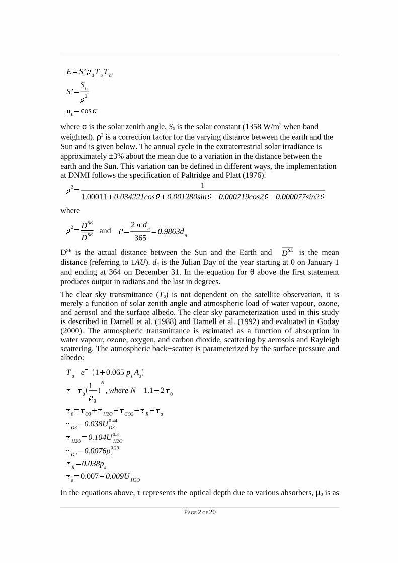
� cos �where σ is the solar zenith angle, S0 is the solar constant (1358 W/m2 when bandweighted). ρ2 is a correction factor for the varying distance between the earth and theSun and is given below. The annual cycle in the extraterrestrial solar irradiance isapproximately ±3% about the mean due to a variation in the distance between theearth and the Sun. This variation can be defined in different ways, the implementationat DNMI follows the specification of Paltridge and Platt (1976).

� 2 � 1

1.00011 � 0.034221cos � � 0.001280sin � � 0.000719cos2 � � 0.000077sin2 �where

� 2 � DSE

DSEand � � 2 � d

n

365� 0.9863d

n

DSE is the actual distance between the Sun and the Earth and DSE is the meandistance (referring to 1AU). dn is the Julian Day of the year starting at 0 on January 1and ending at 364 on December 31. In the equation for θ above the first statementproduces output in radians and the last in degrees.

The clear sky transmittance (Ta) is not dependent on the satellite observation, it ismerely a function of solar zenith angle and atmospheric load of water vapour, ozone,and aerosol and the surface albedo. The clear sky parameterization used in this studyis described in Darnell et al. (1988) and Darnell et al. (1992) and evaluated in Godøy(2000). The atmospheric transmittance is estimated as a function of absorption inwater vapour, ozone, oxygen, and carbon dioxide, scattering by aerosols and Rayleighscattering. The atmospheric back−scatter is parameterized by the surface pressure andalbedo:

Ta

� e� � 1 � 0.065 psA

s

� 0

1�

0

N

,where N � 1.1 2 0

0

� O3

� H2O

� CO2

� R

� a

O3

� 0.038UO3

0.44

H2O

� 0.104UH2O

0.3

O2

� 0.0076ps

0.29

R

� 0.038ps

a� 0.007 � 0.009U

H2O

In the equations above, τ represents the optical depth due to various absorbers, µ0 is as

PAGE 2 OF 20

before the cosine of the solar zenith angle, ps is the nominal surface atmosphericpressure in atmospheres and U is the atmospheric load (in cm) of various constituents.

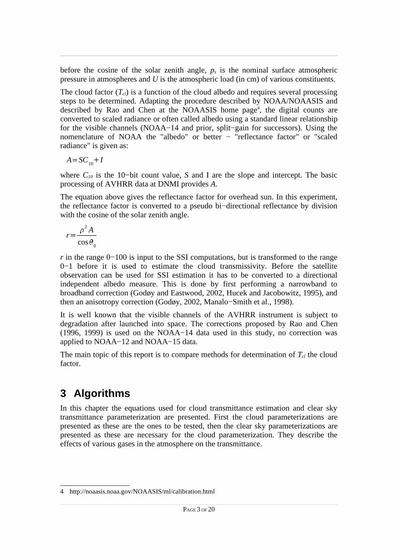
The cloud factor (Tcl) is a function of the cloud albedo and requires several processingsteps to be determined. Adapting the procedure described by NOAA/NOAASIS anddescribed by Rao and Chen at the NOAASIS home page4, the digital counts areconverted to scaled radiance or often called albedo using a standard linear relationshipfor the visible channels (NOAA−14 and prior, split−gain for successors). Using thenomenclature of NOAA the "albedo" or better − "reflectance factor" or "scaledradiance" is given as:

A � SC10

� I

where C10 is the 10−bit count value, S and I are the slope and intercept. The basicprocessing of AVHRR data at DNMI provides A.

The equation above gives the reflectance factor for overhead sun. In this experiment,the reflectance factor is converted to a pseudo bi−directional reflectance by divisionwith the cosine of the solar zenith angle.

r � � 2 A

cos �0

r in the range 0−100 is input to the SSI computations, but is transformed to the range0−1 before it is used to estimate the cloud transmissivity. Before the satelliteobservation can be used for SSI estimation it has to be converted to a directionalindependent albedo measure. This is done by first performing a narrowband tobroadband correction (Godøy and Eastwood, 2002, Hucek and Jacobowitz, 1995), andthen an anisotropy correction (Godøy, 2002, Manalo−Smith et al., 1998).

It is well known that the visible channels of the AVHRR instrument is subject todegradation after launched into space. The corrections proposed by Rao and Chen(1996, 1999) is used on the NOAA−14 data used in this study, no correction wasapplied to NOAA−12 and NOAA−15 data.

The main topic of this report is to compare methods for determination of Tcl the cloudfactor.

3 AlgorithmsIn this chapter the equations used for cloud transmittance estimation and clear skytransmittance parameterization are presented. First the cloud parameterizations arepresented as these are the ones to be tested, then the clear sky parameterizations arepresented as these are necessary for the cloud parameterization. They describe theeffects of various gases in the atmosphere on the transmittance.

4 http://noaasis.noaa.gov/NOAASIS/ml/calibration.html

PAGE 3 OF 20

3.1 Cloud transmittance

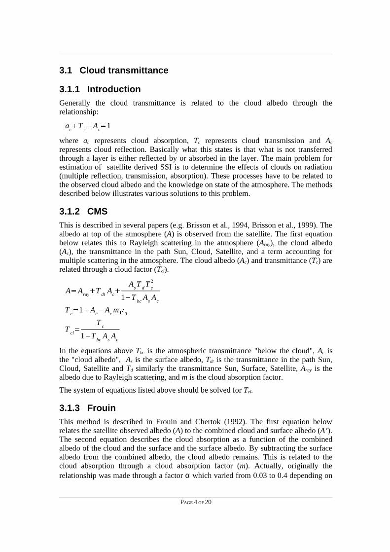
3.1.1 IntroductionGenerally the cloud transmittance is related to the cloud albedo through therelationship:

ac

� Tc

� Ac

� 1

where ac represents cloud absorption, Tc represents cloud transmission and Ac

represents cloud reflection. Basically what this states is that what is not transferredthrough a layer is either reflected by or absorbed in the layer. The main problem forestimation of satellite derived SSI is to determine the effects of clouds on radiation(multiple reflection, transmission, absorption). These processes have to be related totheobserved cloud albedo and theknowledge on stateof theatmosphere. Themethodsdescribed below illustrates various solutions to this problem.

3.1.2 CMSThis is described in several papers (e.g. Brisson et al., 1994, Brisson et al., 1999). Thealbedo at top of the atmosphere (A) is observed from the satellite. The first equationbelow relates this to Rayleigh scattering in the atmosphere (Aray), the cloud albedo(Ac), the transmittance in the path Sun, Cloud, Satellite, and a term accounting formultiple scattering in the atmosphere. The cloud albedo (Ac) and transmittance (Tc) arerelated through a cloud factor (Tcl).

A � Aray

� Tdt

Ac

� AsT

dT

c

2

1 Tbc

AsA

c

Tc

� 1 Ac

Acm �

0

Tcl

� Tc

1 Tbc

AsA

c

In the equations above Tbc is the atmospheric transmittance "below the cloud", Ac isthe "cloud albedo", As is the surface albedo, Tdt is the transmittance in the path Sun,Cloud, Satellite and Td similarly the transmittance Sun, Surface, Satellite, Aray is thealbedo due to Rayleigh scattering, and m is the cloud absorption factor.

The system of equations listed above should be solved for Tcl.

3.1.3 FrouinThis method is described in Frouin and Chertok (1992). The first equation belowrelates the satellite observed albedo (A) to the combined cloud and surface albedo (A’ ).The second equation describes the cloud absorption as a function of the combinedalbedo of the cloud and the surface and the surface albedo. By subtracting the surfacealbedo from the combined albedo, the cloud albedo remains. This is related to thecloud absorption through a cloud absorption factor (m). Actually, originally therelationship was made through a factor α which varied from 0.03 to 0.4 depending on

PAGE 4 OF 20

cloud liquid water content and the solar zenith angle (increasing zenith and liquidwater gives decreasing α). In this implementation it is only affected by thesolar zenithangle, but is confined within the limits specified. The third equation represents thecloud factor, the effect of clouds on the irradiance that reach the surface.

A � Aray

� Tdt

A’

1 SaA’

ac

� m �0

A’ As

Tcl

� 1 A’ ac

1 SaA’

In the equations above A’ is the combined cloud and surface albedo, ac is the cloudabsorption, As is the surface albedo, Td is the Sun−Surface−Satellite transmittance andTdt is the Sun−Cloud−Satellite transmittance. Aray represents the contribution ofscattering in a clear atmosphere to the observed albedo. No formula is given for Aray,

thus the formulation for Rayleigh scattering given by Brisson et al. (1999) was used.TdtA’(1−Saa’)−1 represents the contribution from multiple scattering in the cloud. Sa isthe spherical albedo and accounts for multiple reflection between the surface and thecloud.

In this configuration Tcl in fact represents the ratio between the irradiance that reachesthe surface and the irradiance that would have reached the surface under cloud freeconditions, or rather if the cloud layer and surface were non reflecting and nonabsorbing. In other words this is the combined effect of absorption in the cloud andreflection by the cloud (and surface) on the incoming radiation. This ratio depends onthe solar zenith angle.

3.1.4 Frouin & CMSIn this method the cloud factor (Tcl) formalism of Frouin and Chertok (1992) havebeen used together with the atmospheric transmittance formalism of CMS (e.g.Brisson et al., 1999).

3.2 Atmospheric transmittancesThe equations given in the previous chapter requires specification of absorption due tovarious atmospheric constituents. The formalism used is given below. T? represents asbefore a transmittance, a? represents an absorption, A? an albedo, and U? an amount ofabsorbing matter in cm. Other variables used should be self explained in the set up ofequations.

PAGE 5 OF 20

3.2.1 CMS

Td

� 1 aO3

UO3

1� �0

� 1� � aH2O

UWV

1� �0

� 1� � Aray

�0

A’ray

�T

dt� 1 a

O3U

O31� �

0� 1� � a

H2O0.3U

WV1� �

0� 1� � A

ray�

0 A’

ray�

Aray

�0

� 0.28

1 � 6.43 �0

where

Ta

� � 1 aH2O

UWV

� �0

aO3

UO3

� �0

Aray

aH2O

UWV

� �0

� 2.9 UWV

� �0

1 � 141.5UWV

� �0

0.635� 5.925U

WV� �

0

aO3

x � aO3

VIS x � aO3

UV x x � UO3

� �0

aO3

VIS x � 0.02118x

1 � 0.042x � 0.000323x2

aO3

UV x � 1.082x

1 � 138.6x 0.805� 0.0658x

1 � 103.6x 3

Aray

� 0.28

1 � 6.43 �0

� � e� 0.091� �0 � 0.091

Ta above is not used as the clear sky transmittance is calculated using the Staylorparameterization (Darnell et al., 1988, Darnell et al., 1992), it is only presented for afull specification.

3.2.2 Frouin

d�

O3U

O31� �

0� 1� � �

H2OU

WV1� �

0� 1� � �

sc1� �

0� 1� �

dt

� O3

UO3

1� �0

� 1� � � H2O

0.3UWV

1� �0

� 1� � � sc

1� �0

� 1� �

Td

� e� � d

Tdt

� e� � dt

where

PAGE 6 OF 20

Ta

� e� � H2O e� � O3 e� � sc

1 As

a’ � b’ � V

H2O� 0.102 U

WV� �

0

0.29

O3

� 0.041 UO3

� �0

0.57

sc

� a � b� V �0

maritime: a � 0.059b � 0.359a’ � 0.089b’ � 0.503continental: a � 0.066b � 0.704a’ � 0.088b’ � 0.456

Ta above is not used as the clear sky transmittance is calculated using the Staylorparameterization, it is only presented for a full specification.

4 Experiment set up

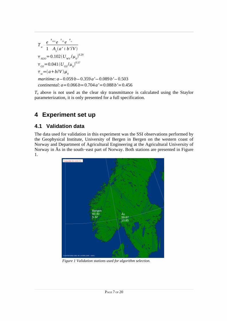
4.1 Validation dataThe dataused for validation in this experiment was the SSI observations performed bythe Geophysical Institute, University of Bergen in Bergen on the western coast ofNorway and Department of Agricultural Engineering at the Agricultural University ofNorway in Ås in the south−east part of Norway. Both stations are presented in Figure1.

PAGE 7 OF 20

Figure 1 Validation stations used for algorithm selection.

Ås59.6710.85

Bergen60.405.32

PLANTEFORSK 2002−06−14 0000 (2300 − 0100 )

Fredag 2002−06−14 00 UTC

PLANTEFORSK 2002−06−14 0000 (2300 − 0100 )

Fredag 2002−06−14 00 UTC

4.2 AVHRR dataThe results presented in this report have been created using two different approachesat different times in the project period. These are denoted as two differentexperiments, but the input AVHRR data were the same.

The AVHRR data used for this study at DNMI was processed from HRPT to level 2by processing software delivered by Kongsberg Spacetec A/S. The level 2 data usedwere radiometrically and geometrically corrected and given on a Polar Stereographicmap projection (correct at 60°N, no rotation) at pixel size 1.5 km. Data wereoutput ona NCSA HDF version 4.2 format.

The first experiment set up in autumn 1999 used data spanning March − September1999. In this experiment the AVHRR data were averaged over 10×10 pixel largeboxes surrounding the validation stations and used as input to the cloud mask. Thecloud covered boxes were used for SSI computations and the results were comparedwith validation data.

In the second experiment, performed in spring 2002 but using the same data period asin the previous experiment, the cloud mask was applied to each pixel on fullresolution. Then SSI computations were performed and the results were averaged on13×13 pixel large boxes before comparison with validation data.

4.3 Cloud maskA very simple cloud mask using AVHRR data only was used for cloud masking inboth experiments. The main features used were:

� A2/A1 > 1� T4 > 0

No information on cloud cover were available from the validation data sets.

4.4 Atmospheric gasesFor both experiments climatological values of atmospheric ozone and water vapourload were used and of surface albedo. The climatological values for Bergen was fromthe actual site while the data for Ås was collected for the Gardermoen airport, about80 km further north, but in a similar landscape. However, there was one majordifference between the first and second experiment. During the first experimentautumn 1999, the surface albedo used for SSI computations at Ås were the actualobserved values at the station, while climatological values were used in the secondexperiment (making the processing similar at Ås and Bergen).

5 Results

5.1 IntroductionAs mentioned above, two different set−ups have been used to evaluate the algorithms.The first experiment performed in autumn 1999 used box (10×10 pixels) averaged

PAGE 8 OF 20

AVHRR data surrounding each validation station (and observed surface albedo forNLH). No figures are provided for this experiment, but statistical values are presentedin a table in Chapter 5.6. The second experiment was performed in spring 2002, usingthesame AVHRR dataas in the first experiment, but now thealgorithms wereused oneach individual pixel instead of on the box average. Then the flux estimates wereaveraged and compared to the validation data. The box size changed between the twoexperiments, being 10×10 in the first and 13×13 in the last. Results from this lastexperiment is also presented in tabular form in Chapter 5.6. In the first experiment thenarrowband to broadband correction scheme was also varied along with the cloudfactor algorithms. In the second experiment, the NOAA scene and cloud dependentcorrection was chosen and applied to all data.

The methods described in Chapter 3 were successively used with the experiment setup described in Chapter 4. Concerning the CMS method, two different cloudabsorption factors were used for this method. These are specified as CMS 0.1 andCMS 0.4 in the presentation of the results for the second experiment. During the firstexperiment only results for a cloud absorption factor of 0.4 is presented in the table forthe CMS method.

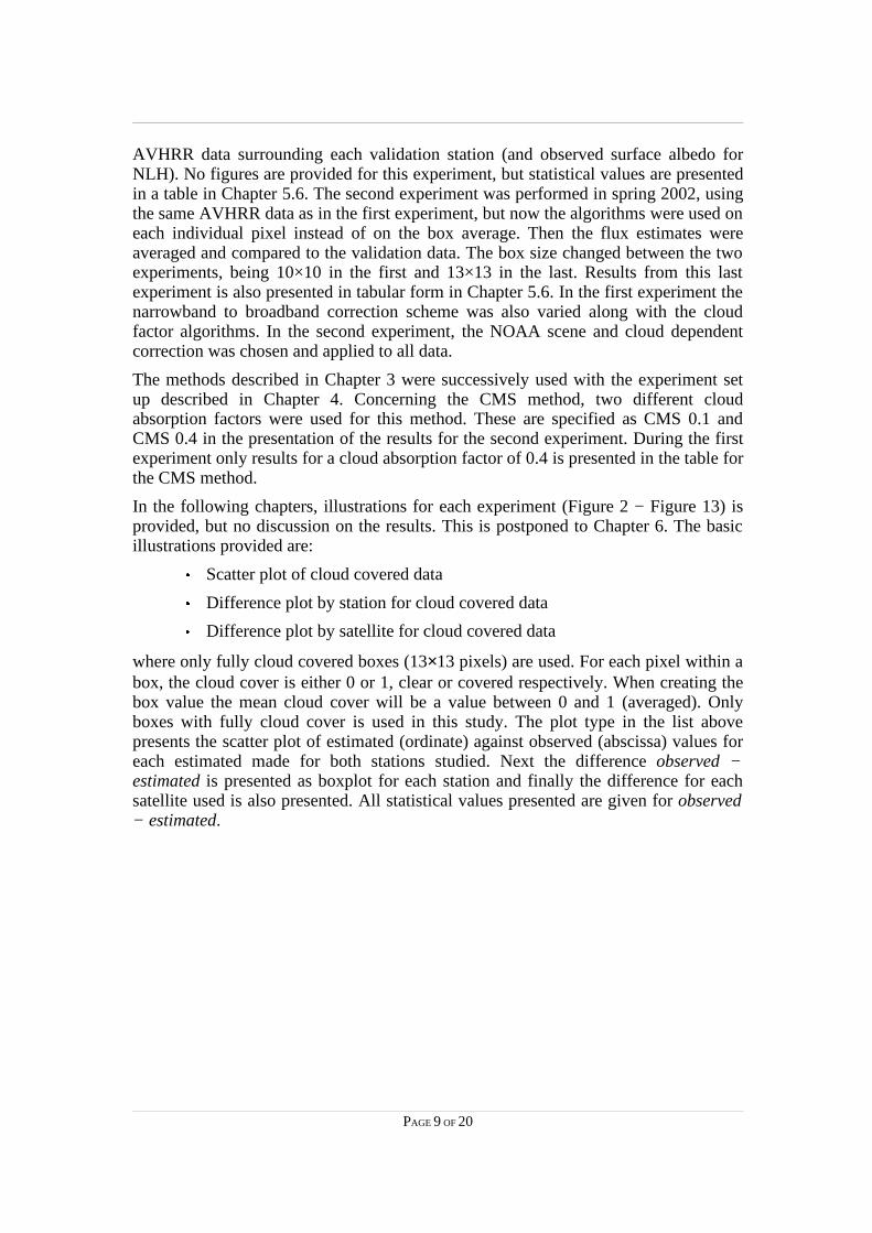
In the following chapters, illustrations for each experiment (Figure 2 − Figure 13) isprovided, but no discussion on the results. This is postponed to Chapter 6. The basicillustrations provided are:

� Scatter plot of cloud covered data� Difference plot by station for cloud covered data� Difference plot by satellite for cloud covered data

where only fully cloud covered boxes (13×13 pixels) are used. For each pixel within abox, the cloud cover is either 0 or 1, clear or covered respectively. When creating thebox value the mean cloud cover will be a value between 0 and 1 (averaged). Onlyboxes with fully cloud cover is used in this study. The plot type in the list abovepresents the scatter plot of estimated (ordinate) against observed (abscissa) values foreach estimated made for both stations studied. Next the difference observed −estimated is presented as boxplot for each station and finally the difference for eachsatellite used is also presented. All statistical values presented are given for observed− estimated.

PAGE 9 OF 20

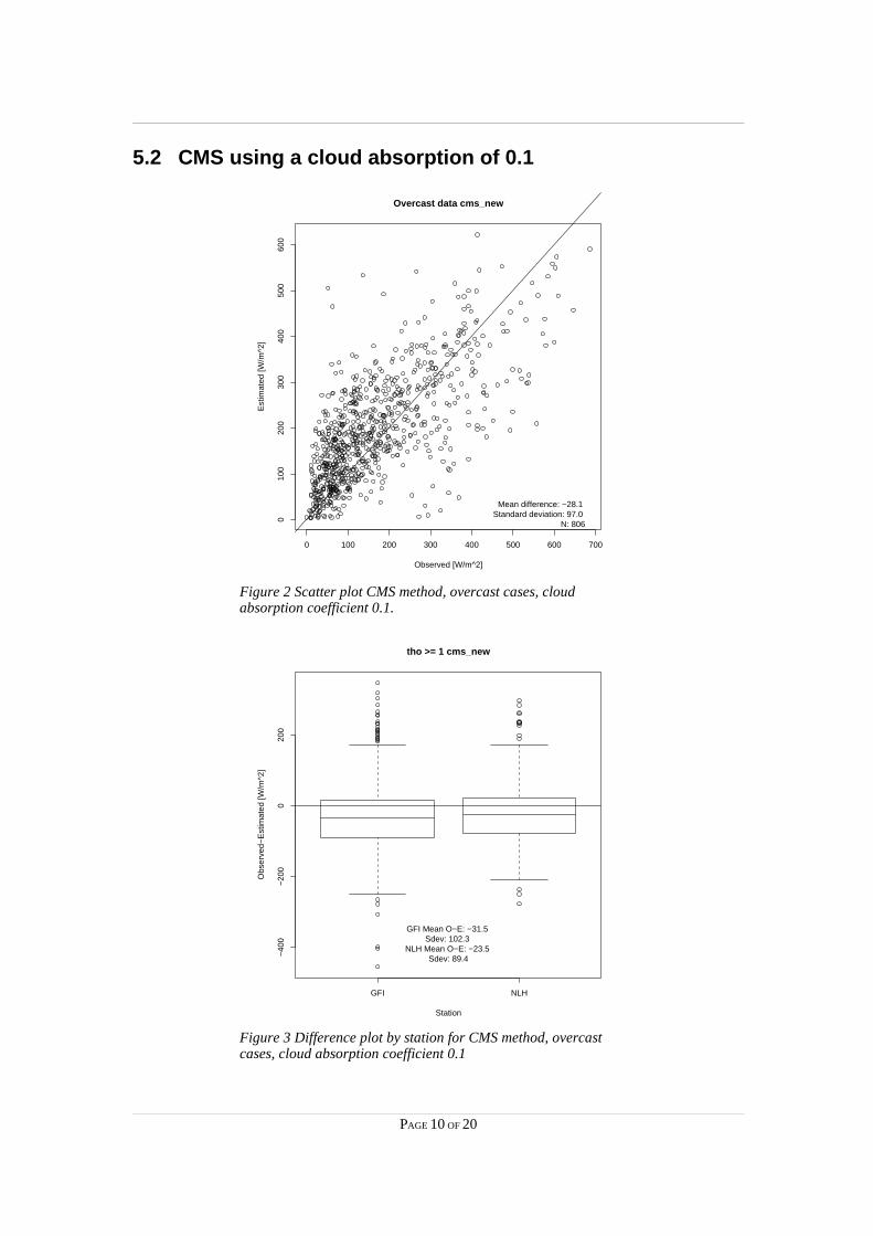
5.2 CMS using a cloud absorption of 0.1

Figure 2 Scatter plot CMS method, overcast cases, cloudabsorption coefficient 0.1.

Figure 3 Difference plot by station for CMS method, overcastcases, cloud absorption coefficient 0.1

PAGE 10 OF 20

0 100 200 300 400 500 600 700

010

020

030

040

050

060

0

Observed [W/m^2]

Est

imat

ed [W

/m^2

]

Overcast data cms_new

Mean difference: −28.1 Standard deviation: 97.0

N: 806

GFI NLH

−40

0−

200

020

0

Station

Obs

erve

d−E

stim

ated

[W/m

^2]

tho >= 1 cms_new

GFI Mean O−E: −31.5 Sdev: 102.3

NLH Mean O−E: −23.5 Sdev: 89.4

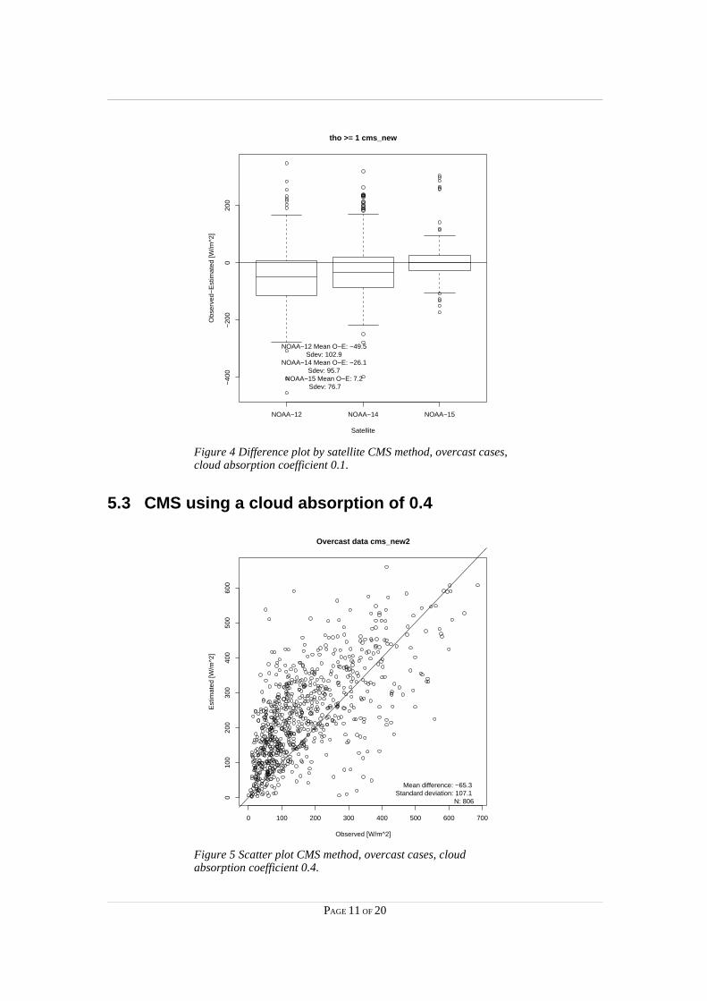
Figure 4 Difference plot by satellite CMS method, overcast cases,cloud absorption coefficient 0.1.

5.3 CMS using a cloud absorption of 0.4

Figure 5 Scatter plot CMS method, overcast cases, cloudabsorption coefficient 0.4.

PAGE 11 OF 20

NOAA−12 NOAA−14 NOAA−15

−40

0−

200

020

0

Satellite

Obs

erve

d−E

stim

ated

[W/m

^2]

tho >= 1 cms_new

NOAA−12 Mean O−E: −49.5 Sdev: 102.9

NOAA−14 Mean O−E: −26.1 Sdev: 95.7

NOAA−15 Mean O−E: 7.2 Sdev: 76.7

0 100 200 300 400 500 600 700

010

020

030

040

050

060

0

Observed [W/m^2]

Est

imat

ed [W

/m^2

]

Overcast data cms_new2

Mean difference: −65.3 Standard deviation: 107.1

N: 806

Figure 6 Difference plot by station CMS method, overcast cases,cloud absorption coefficient 0.4.

Figure 7 Difference plot by satellite − CMS method, overcastcases, cloud absorption coefficient 0.4.

PAGE 12 OF 20

NOAA−12 NOAA−14 NOAA−15

−40

0−

200

020

0

Satellite

Obs

erve

d−E

stim

ated

[W/m

^2]

tho >= 1 cms_new2

NOAA−12 Mean O−E: −73.1 Sdev: 111.1

NOAA−14 Mean O−E: −75.8 Sdev: 107.4

NOAA−15 Mean O−E: −20.2 Sdev: 85.3

GFI NLH

−40

0−

200

020

0

Station

Obs

erve

d−E

stim

ated

[W/m

^2]

tho >= 1 cms_new2

GFI Mean O−E: −69.1 Sdev: 112.7

NLH Mean O−E: −60.3 Sdev: 99.0

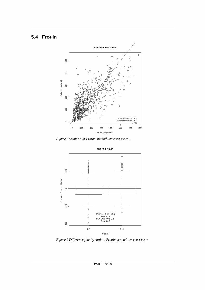
5.4 Frouin

Figure 8 Scatter plot Frouin method, overcast cases.

Figure 9 Difference plot by station, Frouin method, overcast cases.

PAGE 13 OF 20

GFI NLH

−40

0−

200

020

0

Station

Obs

erve

d−E

stim

ated

[W/m

^2]

tho >= 1 frouin

GFI Mean O−E: −12.5 Sdev: 93.9

NLH Mean O−E: 0.8 Sdev: 86.3

0 100 200 300 400 500 600 700

010

020

030

040

050

0

Observed [W/m^2]

Est

imat

ed [W

/m^2

]

Overcast data frouin

Mean difference: −6.7 Standard deviation: 90.9

N: 792

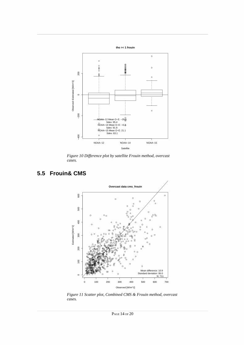
Figure 10 Difference plot by satellite Frouin method, overcastcases.

5.5 Frouin& CMS

Figure 11 Scatter plot, Combined CMS & Frouin method, overcastcases.

PAGE 14 OF 20

NOAA−12 NOAA−14 NOAA−15

−40

0−

200

020

0

Satellite

Obs

erve

d−E

stim

ated

[W/m

^2]

tho >= 1 frouin

NOAA−12 Mean O−E: −29.5 Sdev: 95.4

NOAA−14 Mean O−E: −0.3 Sdev: 91.9

NOAA−15 Mean O−E: 21.1 Sdev: 63.1

0 100 200 300 400 500 600 700

010

020

030

040

050

060

0

Observed [W/m^2]

Est

imat

ed [W

/m^2

]

Overcast data cms_frouin

Mean difference: 10.9 Standard deviation: 95.0

N: 711

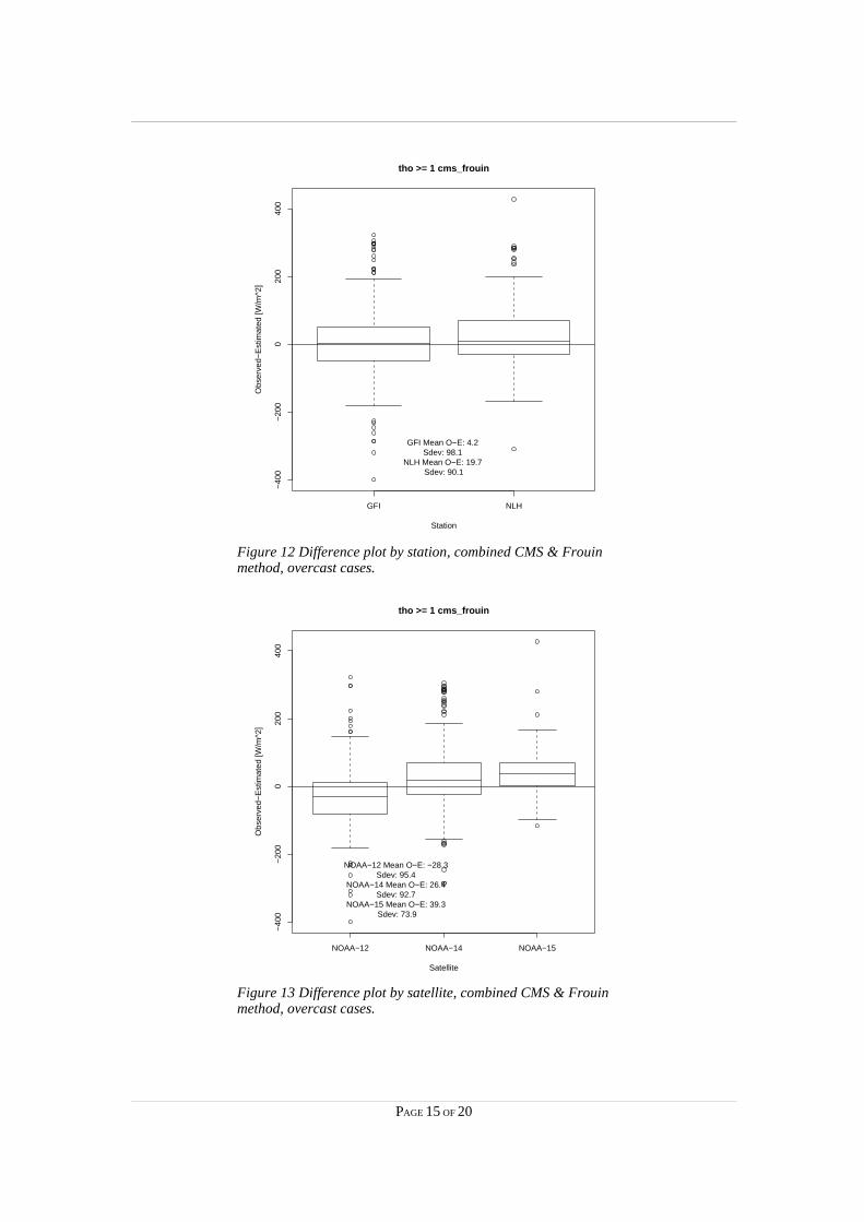
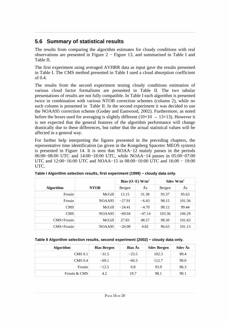
Figure 12 Difference plot by station, combined CMS & Frouinmethod, overcast cases.

Figure 13 Difference plot by satellite, combined CMS & Frouinmethod, overcast cases.

PAGE 15 OF 20

NOAA−12 NOAA−14 NOAA−15

−40

0−

200

020

040

0

Satellite

Obs

erve

d−E

stim

ated

[W/m

^2]

tho >= 1 cms_frouin

NOAA−12 Mean O−E: −28.3 Sdev: 95.4

NOAA−14 Mean O−E: 26.4 Sdev: 92.7

NOAA−15 Mean O−E: 39.3 Sdev: 73.9

GFI NLH

−40

0−

200

020

040

0

Station

Obs

erve

d−E

stim

ated

[W/m

^2]

tho >= 1 cms_frouin

GFI Mean O−E: 4.2 Sdev: 98.1

NLH Mean O−E: 19.7 Sdev: 90.1

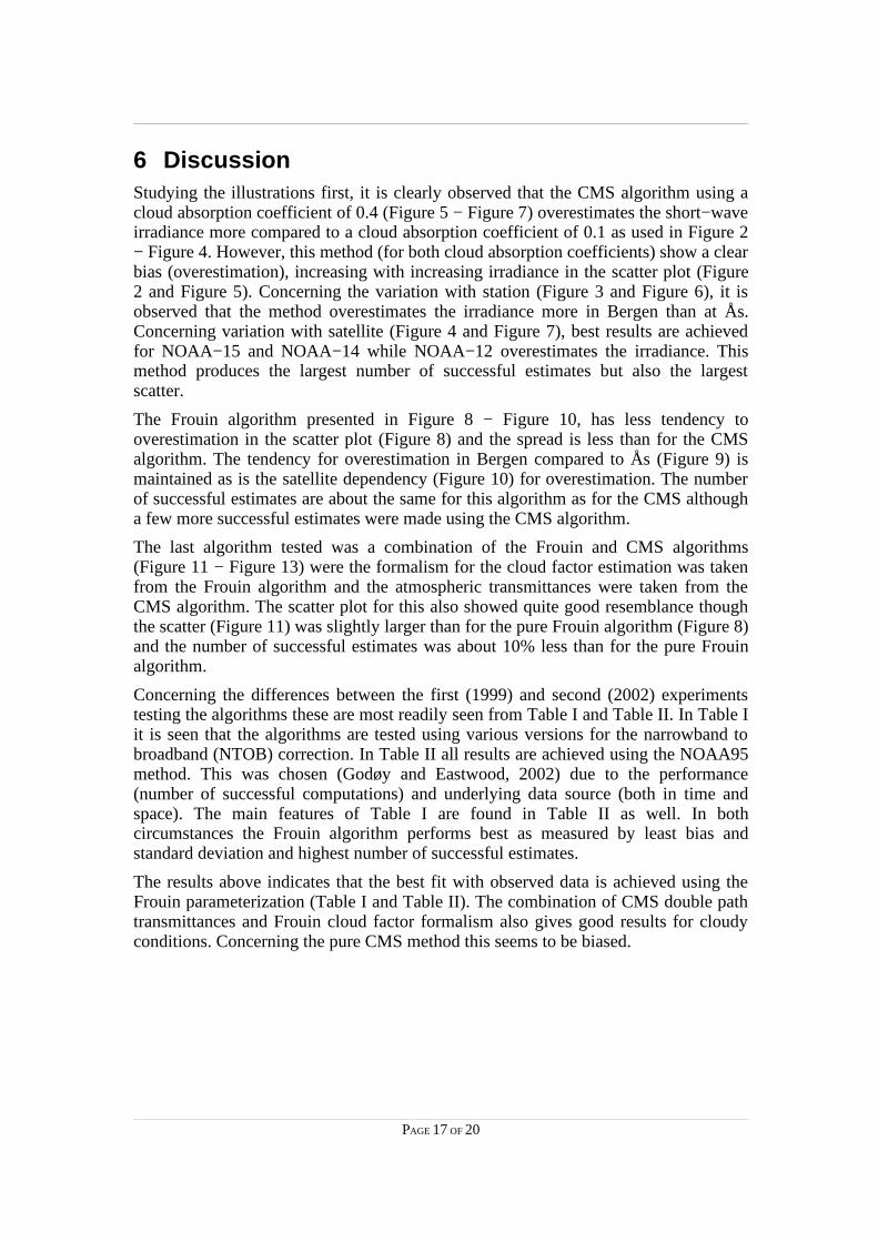
5.6 Summary of statistical resultsThe results from comparing the algorithm estimates for cloudy conditions with realobservations are presented in Figure 2 − Figure 13, and summarised in Table I andTable II.

The first experiment using averaged AVHRR data as input gave the results presentedin Table I. The CMS method presented in Table I used a cloud absorption coefficientof 0.4.

The results from the second experiment testing cloudy conditions estimation ofvarious cloud factor formalisms are presented in Table II. The two tabularpresentations of results arenot fully compatible. In Table I each algorithm is presentedtwice in combination with various NTOB correction schemes (column 2), while nosuch column is presented in Table II. In the second experiment it was decided to usethe NOAA95 correction scheme (Godøy and Eastwood, 2002). Furthermore, as notedbefore the boxes used for averaging is slightly different (10×10 → 13×13). However itis not expected that the general features of the algorithm performance will changedrastically due to these differences, but rather that the actual statistical values will beaffected in a general way.

For further help interpreting the figures presented in the preceding chapters, therepresentative time identification (as given in the Kongsberg Spacetec MEOS system)is presented in Figure 14. It is seen that NOAA−12 mainly passes in the periods06:00−08:00 UTC and 14:00−18:00 UTC, while NOAA−14 passes in 05:00−07:00UTC and 12:00−16:00 UTC and NOAA−15 in 08:00−10:00 UTC and 16:00 − 19:00UTC.

Table I Algorithm selection results, first experiment (1999) − cloudy data only.

Algor ithm NTOB

Bias (O−E) W/m2 Sdev W/m2

Bergen Ås Bergen Ås

Frouin McGill 13.15 31.38 93.37 95.63

Frouin NOAA95 −27.91 −6.43 98.15 101.56

CMS McGill −24.41 −4.70 98.12 99.44

CMS NOAA95 −69.04 −47.14 103.36 106.29

CMS+Frouin McGill 27.83 48.57 98.50 101.63

CMS+Frouin NOAA95 −20.08 4.82 96.63 101.13

Table II Algorithm selection results, second experiment (2002) − cloudy data only.

Algor ithm Bias Bergen Bias Ås Sdev Bergen Sdev Ås

CMS 0.1 −31.5 −23.5 102.3 89.4

CMS 0.4 −69.1 −60.3 112.7 99.0

Frouin −12.5 0.8 93.9 86.3

Frouin & CMS 4.2 19.7 98.1 90.1

PAGE 16 OF 20

6 DiscussionStudying the illustrations first, it is clearly observed that the CMS algorithm using acloud absorption coefficient of 0.4 (Figure 5 − Figure7) overestimates the short−waveirradiance more compared to a cloud absorption coefficient of 0.1 as used in Figure 2− Figure 4. However, this method (for both cloud absorption coefficients) show a clearbias (overestimation), increasing with increasing irradiance in the scatter plot (Figure2 and Figure 5). Concerning the variation with station (Figure 3 and Figure 6), it isobserved that the method overestimates the irradiance more in Bergen than at Ås.Concerning variation with satellite (Figure 4 and Figure 7), best results are achievedfor NOAA−15 and NOAA−14 while NOAA−12 overestimates the irradiance. Thismethod produces the largest number of successful estimates but also the largestscatter.

The Frouin algorithm presented in Figure 8 − Figure 10, has less tendency tooverestimation in the scatter plot (Figure 8) and the spread is less than for the CMSalgorithm. The tendency for overestimation in Bergen compared to Ås (Figure 9) ismaintained as is the satellite dependency (Figure 10) for overestimation. The numberof successful estimates are about the same for this algorithm as for the CMS althougha few more successful estimates were made using the CMS algorithm.

The last algorithm tested was a combination of the Frouin and CMS algorithms(Figure 11 − Figure 13) were the formalism for the cloud factor estimation was takenfrom the Frouin algorithm and the atmospheric transmittances were taken from theCMS algorithm. The scatter plot for this also showed quite good resemblance thoughthescatter (Figure 11) was slightly larger than for the pureFrouin algorithm (Figure8)and the number of successful estimates was about 10% less than for the pure Frouinalgorithm.

Concerning the differences between the first (1999) and second (2002) experimentstesting the algorithms these are most readily seen from Table I and Table II. In Table Iit is seen that the algorithms are tested using various versions for the narrowband tobroadband (NTOB) correction. In Table II all results are achieved using the NOAA95method. This was chosen (Godøy and Eastwood, 2002) due to the performance(number of successful computations) and underlying data source (both in time andspace). The main features of Table I are found in Table II as well. In bothcircumstances the Frouin algorithm performs best as measured by least bias andstandard deviation and highest number of successful estimates.

The results above indicates that the best fit with observed data is achieved using theFrouin parameterization (Table I and Table II). The combination of CMS double pathtransmittances and Frouin cloud factor formalism also gives good results for cloudyconditions. Concerning the pure CMS method this seems to be biased.

PAGE 17 OF 20

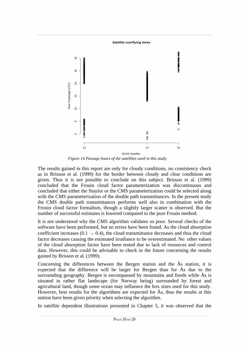
Figure 14 Passage hours of the satellites used in this study.

The results gained in this report are only for cloudy conditions, no consistency checkas in Brisson et al. (1999) for the border between cloudy and clear conditions aregiven. Thus it is not possible to conclude on this subject. Brisson et al. (1999)concluded that the Frouin cloud factor parameterization was discontinuous andconcluded that either the Staylor or the CMS parameterization could be selected alongwith the CMS parameterization of the double path transmittances. In the present studythe CMS double path transmittances performs well also in combination with theFrouin cloud factor formalism, though a slightly larger scatter is observed. But thenumber of successful estimates is lowered compared to the pure Frouin method.

It is not understood why the CMS algorithm validates so poor. Several checks of thesoftware have been performed, but no errors have been found. As the cloud absorptioncoefficient increases (0.1 → 0.4), the cloud transmittance decreases and thus the cloudfactor decreases causing the estimated irradiance to be overestimated. No other valuesof the cloud absorption factor have been tested due to lack of resources and controldata. However, this could be advisable to check in the future concerning the resultsgained by Brisson et al. (1999).

Concerning the differences between the Bergen station and the Ås station, it isexpected that the difference will be larger for Bergen than for Ås due to thesurrounding geography. Bergen is encompassed by mountains and fiords while Ås issituated in rather flat landscape (for Norway being) surrounded by forest andagricultural land, though some ocean may influence the box sizes used for this study.However, best results for the algorithms are expected for Ås, thus the results at thisstation have been given priority when selecting the algorithm.

In satellite dependent illustrations presented in Chapter 5, it was observed that the

PAGE 18 OF 20

NOAA �Satellite

Hou

r of p

assa

ge (U

TC)

68

1012

1416

18

12 14 15

Satellite overflying times

error dependency on satellite indicated that largest errors were found for NOAA−12.This a very old satellite and no compensation for sensor drift have been performed onthe data. For NOAA−14 the correction proposed by NOAA (Rao and Chen, 1996,1999) were applied and updated regularly while no compensation was performed onthe NOAA−15 data. However, the NOAA−15 platform was only about a year oldwhen this study was initiated (launched 13 may 1998). The difference between resultsgained using NOAA−14 and NOAA−15 is not fully understood as NOAA−14 wascompensated and NOAA−15 was a quite new satellite at the time. However, if thesensor degradation of NOAA−14 was not fully corrected a decreasing albedo in timewould cause an overestimation in SSI. Furthermore, as seen in Figure 14 the satellitepassage times for the data used varies between NOAA−14 and NOAA−15, NOAA−15being subject to higher solar zenith angles than NOAA−14 which may affect thequality of estimates.

Good performance on NOAA−14 / NOAA−15 and at Ås were given priority in thealgorithm selection along with low scatter and a high number of successful estimates.Based upon this the Frouin algorithm was selected for use in the Ocean and Sea IceSAF project at high latitudes.

The algorithm selection performed in this study have several drawbacks. Firstclimatological values for atmospheric gases and surface albedo have been use, secondthe cloud mask is very coarse, third the consistency check between clear and cloudycases are lacking. The first 2 objections are not supposed to alter the resultsignificantly as they should produce similar effects for all algorithms. They may affectthe error, but are not expected to change the ranking of algorithms. The consistencycheck is lacking and should be performed in the future when further testing of theCMS algorithm is performed as this could alter the ranking if other cloud absorptioncoefficients improve the CMS validation results.

7 SummaryBased upon the validation results the Frouin parameterization is chosen for the Oceanand Sea Ice SAF estimation of High Latitude surface solar irradiance using AVHRRdata as input. It would be advisable to pursue the CMS parameterization further bytesting various cloud absorption coefficients to achieve consistency between theGOES and POES SSI estimation and to identify any possible inconsistency betweenthe clear and cloudy estimation process. However, at present, the Frouin method isimplemented and tested for full processing of SSI and any further testing of the CMSmethod will be performed first on the data set from 1999, then in a parallel processingchain.

PAGE 19 OF 20

ReferencesBrisson, A., P. Le Borgne, A. Marsouin, and T. Moreau, 1994: Surface irradiancescalculated from Meteosat sensor data during SOFIA−ASTEX, Int. J. Rem. Sens., Vol.15, No. 1, pp. 197−203, 1994.

Brisson, A., P. LeBorgne, and A. Marsouin, 1999: Development of algorithms forSurface Solar Irradiance retrieval at O&SI SAF Low and Mid Latitudes, Internalreport at Météo France/SCEM/CMS, February 1999.

Darnell, W.L., F. Staylor, S.K. Gupta, and F.M. Denn, 1988: Estimation of surfaceinsolation using sun−synchronous satellite data, J. Climate, Vol. pp. 820−835, 1988.

Darnell, W.L., W.F. Staylor, S.K. Gupta, N.A. Ritchey, and A.C. Wilbur, 1992:Seasonal variation of surface radiation budget derived from international satellitecloud climatology project C1 data, J. Geophys. Res., Vol. 97, pp. 15 741 − 15760,1992.

Frouin, R., and B. Chertok, 1992: A Technique for Global Monitoring of Net SolarIrradiance at the Ocean Surface. Part I: Model, J. Appl. Met., Vol. 31, pp. 1056−1066.

Godøy, Ø., and S. Eastwood, 2002a: Narrowband to broadband correction ofNOAA/AVHRR data, DNMI Research Note, No. 68, Norwegian MeteorologicalInstitute, 12pp.

Godøy, Ø., 2002: Anisotropy correction for AVHRR data within the Ocean and SeaIce SAF framework, Report in preparation, Norwegian Meteorological Institute.

Godøy, Ø., 2000: Evaluation of clear sky solar irradiance algorithms at high latitudes,DNMI Research Note, No. 36, Norwegian Meteorological Institute, 13pp.

Hucek, R., and H. Jacobowitz, 1995: Impact of Scene Dependence on AVHRRAlbedo Models, J. Atm. Oce. Tech., Vol. 12, No. 4, pp. 697−711.

Manalo−Smith, N., G. L. Smith, S. N. Tiwari, and W. F. Staylor, 1998: Analyticforms of bi−directional reflectance functions for application to Earth radiation budgetstudies, J. G. R., Vol. 103, No. D16, pp. 19 733−19 751, 1998.

Paltridge, G.W., and C.M.R. Platt, 1976: Radiative processes in Meteorology andClimatology, Elsevier, ISBN 0−444−41444−4.

Rao, C.R.N, and J. Chen, 1999: Revised post−launch calibration of the visible andnear−infrared channels of the Advanced Very High Resolution Radiometer (AVHRR)on the NOAA−14 spacecraft, Int. J. Rem. Sens., Vol. 20, No. 18, pp. 3485−3491.

Rao, C.N.R., and J. Chen, 1996: Post−launch calibration of the visible and near−infrared channels of the Advanced Very High Resolution Radiometer on the NOAA−14 spacecraft, Int. J. Rem. Sens., Vol. 17, pp. 2743−2747.

PAGE 20 OF 20