TESTING FOR STRUCTURAL STABILITY IN THE WHOLE SAMPLE JAVIER HIDALGO AND MYUNG HWAN SEO Abstract. Testing for structural stability has attracted a lot of attention in theoretical and applied research. Oftentimes the test is based on the supremum of, for example, the Wald statistic when the break is assumed to be in the interval [n] <s<n [n] for some > 0 and where n denotes the sample size. More recently there has been some work to allow the possibility that the break lies at the end of the sample, i.e. when s 2 (n s; n) for some nite number s. However, the previous setups do not include the important intermediate case when s 2 ( s; [n]) [(n [n] ;n s), or more generally when we do not wish to assume any prior knowledge on the location of the break. The aim of the paper is thus to extend existing results on stability tests in the later scenario for models useful in economics such as nonlinear simultaneous equations and transformation models. Letting the time of the break to be anywhere in the sample might not only be more realistic in applied research, but it avoids also the unpleasant need to choose either or s. In addition we show that, contrary to the conventional tests, the tests described and examined in the paper are consistent irrespective of the location of the break. JEL Classication: C21, C23. 1. INTRODUCTION Since the work of Chow (1960) and Quandt (1960), testing for structural stability has been a very active topic of theoretical and applied research. The bulk of the research has focused on the situation when the exact time of the break s is not known but the researcher assumes that s lies in the middleof the sample. That is, s 2 ([n ] ;n [n ]) for some trimming quantity > 0, and where herewith n denotes the sample size. See Andrews (1993) or the latest review article by Perron (2006). In this scenario, the location of the break is often parameterized as the fraction = s=n 2 (; 1 ), and it has been shown that the supremum of, for instance, the Wald (W) or Lagrange Multiplier (LM) statistics (denoted herewith as conventional statistics) converge to the supremum of a Gaussian process. More recently, there has been some interest in the case where the break occurs at the endof the sample. For example, Andrews (2003) or Andrews and Kim (2006), and references therein, examined the case when s 2 (n s; n) for some nite value s. In this situation, we know that, although the tests are not consistent and their distributions depend on s, it is still possible to make inferences as it was shown by Andrews (2003). What has not been studied is the case when s 2 ( s; [n ]) or (n [n ] ;n s), or more importantly, when we do not wish to impose any prior knowledge on the location of the break, avoiding the need to choose or s: The paper thus considers the problem of testing for structural stability over the whole sample span s =1; :::; n. That is, when no previous information about the location of the break is available. The test does not involve a trimming quantity Date : 11 November 2008. Key words and phrases. Structural Stability. Nonlinear and transformation models. GMM estimation. Strong approximation. Extreme value distributions. Ornstein-Uhlenbeck process. 1

Welcome message from author
This document is posted to help you gain knowledge. Please leave a comment to let me know what you think about it! Share it to your friends and learn new things together.
Transcript

TESTING FOR STRUCTURAL STABILITY IN THE WHOLESAMPLE
JAVIER HIDALGO AND MYUNG HWAN SEO
Abstract. Testing for structural stability has attracted a lot of attention intheoretical and applied research. Oftentimes the test is based on the supremumof, for example, the Wald statistic when the break is assumed to be in theinterval [�n] < s < n � [�n] for some � > 0 and where n denotes the samplesize. More recently there has been some work to allow the possibility thatthe break lies at the end of the sample, i.e. when s 2 (n��s; n) for some�nite number �s. However, the previous setups do not include the importantintermediate case when s 2 (�s; [�n])[(n� [�n] ; n��s), or more generally whenwe do not wish to assume any prior knowledge on the location of the break.The aim of the paper is thus to extend existing results on stability tests in thelater scenario for models useful in economics such as nonlinear simultaneousequations and transformation models. Letting the time of the break to beanywhere in the sample might not only be more realistic in applied research,but it avoids also the unpleasant need to choose either � or �s. In addition weshow that, contrary to the conventional tests, the tests described and examinedin the paper are consistent irrespective of the location of the break.
JEL Classi�cation: C21, C23.
1. INTRODUCTION
Since the work of Chow (1960) and Quandt (1960), testing for structural stabilityhas been a very active topic of theoretical and applied research. The bulk of theresearch has focused on the situation when the exact time of the break s is notknown but the researcher assumes that s lies in the �middle�of the sample. Thatis, s 2 ([n� ] ; n� [n� ]) for some trimming quantity � > 0, and where herewith ndenotes the sample size. See Andrews (1993) or the latest review article by Perron(2006). In this scenario, the location of the break is often parameterized as thefraction � = s=n 2 (� ; 1� �), and it has been shown that the supremum of, forinstance, the Wald (W) or Lagrange Multiplier (LM) statistics (denoted herewithas conventional statistics) converge to the supremum of a Gaussian process. Morerecently, there has been some interest in the case where the break occurs at the�end�of the sample. For example, Andrews (2003) or Andrews and Kim (2006),and references therein, examined the case when s 2 (n��s; n) for some �nite value�s. In this situation, we know that, although the tests are not consistent and theirdistributions depend on �s, it is still possible to make inferences as it was shownby Andrews (2003). What has not been studied is the case when s 2 (�s; [n� ]) or(n� [n� ] ; n��s), or more importantly, when we do not wish to impose any priorknowledge on the location of the break, avoiding the need to choose � or �s:The paper thus considers the problem of testing for structural stability over the
whole sample span s = 1; :::; n. That is, when no previous information about thelocation of the break is available. The test does not involve a trimming quantity
Date : 11 November 2008.Key words and phrases. Structural Stability. Nonlinear and transformation models. GMM
estimation. Strong approximation. Extreme value distributions. Ornstein-Uhlenbeck process.
1

2 JAVIER HIDALGO AND MYUNG HWAN SEO
and it can be applied to models useful in economics, such as nonlinear simultaneousequations and transformation models under general conditions on the dependencestructure of the variables of the model. In particular, we do not need to assumethat the data, for instance the regressors and error term in a regression model,are covariance stationary. In this way, we substantially extend Horvath�s (1993)results who only examines this problem for the mean of otherwise independent andnormally distributed random variables.In our setup, Andrews (1993) showed that the conventional tests diverge to in-
�nity without trimming, signalling that the trimming was not only imposed fortechnical convenience but it was also crucial to obtain a proper asymptotic distrib-ution. We show that the reason for his �nding is because the normalization that werequire for the statistic is di¤erent to that for the conventional tests. We also showthat the asymptotic distribution of our tests is di¤erent to that of the conventionaltest. More speci�cally, we show that, after appropriate normalization, which is onlya simple function of the sample size n and the number of parameters subject tobreak, the sups=1;:::;nW (s) and sups=1;:::;n LM (s) test statistics converge to theType I Extreme Value Distribution or Gumbel distribution.It is also worth mentioning that as Andrews and Ploberger (1994) discussed, to
obtain their optimality results, we need to be away from (or not too close to) thebeginning or the end of the sample. Indeed, the Monte-Carlo experiment in Sec-tion 4 suggests that when we compare the power of the conventional tests againstthe power of our tests in Sections 2 and 3, the assumptions made in Andrewsand Ploberger (1994) were not innocuous. More speci�cally, as Section 2.3 shows,the conventional tests are not consistent when the break occurs at time s � n1=2
or n � n1=2 < s, whereas our tests are always consistent irrespective of the loca-tion of the break. In addition, we show that when the break falls in the region
s 2�n1=2; n= (log log n)
1=2�, the conventional tests have zero asymptotic relative
e¢ ciency compared to ours, in the sense that our tests are able to detect localalternatives that, for instance, the �optimal conventional tests�would not do. It isworth mentioning that our tests are similar as that of Brown, Durbin and Evans(1975), in the sense that they do not trim. However, the latter work su¤ers fromthe same lack of power just described for the conventional tests.We �nish this section discussing some theoretical and practical issues regarding
our tests in Sections 2 or 3 below when they are compared with conventional tests.From a practical point of view, our tests have the bene�t that the practitionerdoes not need to choose the rather arti�cial quantities � or �s when performing thetest. Moreover, we avoid the rather undesirable outcome that, even when using thesame data set, two practitioners may lead to contradictory conclusions by choosingtwo di¤erent values of � . This is con�rmed in the small Monte-Carlo experimentdescribed in Section 4, which suggests that the choice of � is not irrelevant byobserving that the size and power of the test vary with the choice of � . In fact, ifwe followed the recommendation given by some authors of taking � = :15, see forinstance Andrews (1993), the power of the conventional test is much lower whenit is compared to our test or when we choose � = :05, although when the break istowards the end of the sample our test is preferable.The remainder of the paper is organized as follows. For exposition purposes,
next section describes and establishes the asymptotic distribution of the tests ina linear regression model, whereas Section 3 extends the results to more generalmodels useful in econometrics such as nonlinear simultaneous equation systems andtransformation models. Section 4 describes a Monte-Carlo experiment to examine

TESTING FOR STRUCTURAL BREAKS 3
the �nite sample performance of our tests and how they compare with the conven-tional tests for some values of � . Finally, Section 5 gives the proofs of our mainresults in Sections 2 and 3.
2. TESTS FOR BREAKS
This section examines, for exposition purposes, tests for breaks in the linearregression model
(2.1) yt = �+ �0xt + �0zt (s) + ut, t = 1; :::; n
where, denoting 1 (�) as the indicator function,
(2.2) zt (s) = xt11 (t � s)
being xt1 a p1 subvector of the p-dimensional vector xt = (x0t1; x0t2)
0 and wherefutgt2Z is a zero mean sequence of errors. Our null hypothesis H0 of interest isthat the parameter � is zero for all s. That is,
(2.3) H0 : � = 0 8s : p� < s � n� p�,
where p� = p+p1+1, being the alternative hypothesis H1 the negation of the null,that is
H1 : 9s : p� < s � n� p�; � 6= 0.Notice that when p1 = p (and zt also includes the intercept), we have that (2:3)
corresponds to the so-called pure structural break hypothesis testing. We considerthe situation under the alternative of a one-time structural break, although as wewill see in Section 2.3 below, the tests have non-trivial power when the break isgradual and it takes some periods for the model or parameters to reach its newregime. In addition, we have assumed for simplicity that the intercept is constant.It goes without saying that our results follow if we allow the intercept to be subjectto a possible break. The only di¤erence lies in the computation of the test and morespeci�cally on the estimation of the asymptotic covariance matrix of the estimatorof the intercept. The same comments would apply if the regression model had atime trend subject to a possible break.We now describe the estimators and present some notation to be used throughout
the paper. Herewith C denotes a generic �nite positive constant. For a genericsequence fwtgnt=1, we write f ewtgnt=1 =: fwt � wgnt=1, where w = n�1
Pnt=1 wt.
Also,
(2.4) Wn = ( ew1; :::; ewn)0 ,which may have a partition Wn =
�W1n
...W2n
�. For a �xed s 2 (p�; n�p�], Wn (s)
indicates that ewt is obtained from wt1 (t � s) and we denote the least squaresestimator of
��0; �0
�0in (2:1) by
(2.5)
b�(s)b�(s)!=
�Z 0n (s)Zn (s) Z 0n (s)Xn
X 0nZn (s) X 0
nXn
��1�Z 0n (s)YnX 0nYn
�.
We should mention that if, for example, the matrix Z 0n (s)Zn (s) were singular,in the computation of our estimates and/or tests, we would use the generalizedinverse instead of the inverse. This will not a¤ect any of the conclusions of thepaper. Similar comments apply elsewhere below.We now introduce the following assumptions.
4 JAVIER HIDALGO AND MYUNG HWAN SEO
A1: fxtgt2Z and futgt2Z are two linear processes de�ned by
xt = �x +1Xi=0
�i"t�i,1Xi=0
k�ik1=&
<1 and �0 = Ip
ut =1Xi=0
�i�t�i,1Xi=0
j�ij1=&
<1 and �0 = 1,
for some & � 3=2, where f"tgt2Z and f�tgt2Z are mutually independentsequences of independently distributed zero mean random variables suchthat E
��2t�= �2� and E ("t"0t) = �" and supt E kxtk
4+ supt E jutj
4< 1,
where kAk denotes the Euclidean norm of the matrix A and Ip is the p-dimensional identity matrix.
Denote Ms =Pst=1 extex0t. Then,
A2: s�1Ms !s!1 � > 0.
A1 is restrictive in the assumption of linearity, although as we shall see in thenext section, we can relax this requirement to allow for more general sequences ofrandom variables. The condition on the rate of convergence to zero of f�igi�0 andf�igi�0 is minimal and it implies that �i and �i are o
�i�3=2
�. The assumption of
identical second moments is not essential for the results to follow, but for exposi-tional purposes we have assumed that the sequences fxtgt2Z and futgt2Z are covari-ance stationary. In fact, we can allow the sequences fxtgt2Z and futgt2Z to exhibitheterogeneity, so that we could allow for heteroscedastic errors E
�u2t jxt
�= �2 (xt),
and hence we do not need to assume that the sequences fxtgt2Z and futgt2Z are mu-tually independent. More explicitly, see Andrews (1993) or Bai and Perron (1998)among others, it would su¢ ce to assume that
(2.6) V ar
0@n�1=2 [n�2]Xt=[n�1]+1
(xt � �x)ut
1A! (�2 � �1) �,
where � = limn!1 n�1 var (Pnt=1 (xt � �x)ut). We keep nevertheless in this sec-
tion Assumption A1 as it stands for pedagogical reasons to make the proof ofProposition 1 below clearer while, at the same time, keeping the main steps formore general type of data and models examined in Section 3. We shall neverthelessemphasize that we do not assume anywhere that the sequences fxtgt2Z or futgt2Zare stationary.Before we present the test for the null hypothesis H0 in (2:3), we put forward a
proposition which plays a key role in the proof of Theorem 1 below.
Proposition 1. Under A1 and A2 , we can construct on a probability space ap-dimensional Wiener process B (k) with independent components such that
(2.7) Pr
(sup
1�k�n
kXt=1
(xt � �x)ut � �1=2k B (k)
> a
)� Ca�4n
�+2(�+1) ,
for some 1 < � < 2, and where �k = k�1 var�Pk
t=1 (xt � �x)ut�.
Proposition 1 extends previous results by Einmahl (1989) who considered partialsums of a vector sequence of independent identically distributed random variablesor those in Götze and Zaitsev (2007) for nonidentically distributed sequences ofindependent random variables. The latter work is an extension to vector sequencesof results due to Sakhanenko, see for instance Shao (1995). Observe that the rateof the approximation in (2:7) is worse than the �standard�n1=4 for linear sequencesof random variables or scalar nonlinear sequences of random variables, as shown

TESTING FOR STRUCTURAL BREAKS 5
respectively by Wang, Lin and Gulati (2003) and Wu (2007). It is worth indicat-ing that if the sequence fxtgt2Z were deterministic, we would have the standardconclusion of the order of approximation to be n1=4.We now comment on the key role that Proposition 1 plays on our results. Take for
example the Wald statistic in (2:10) or (2:12) below. Inspecting its formulation andusing the notation Ss =
Pst=1 (xt � �x)ut, the asymptotic distribution depends on
that of (n= (n� s))1=2 s�1=2e�(s), which is governed by the behaviour of�n
n� s
�1=21
s1=2
�Ip1...0p1�p�p1
�nSs �
s
nSn
o=
�Ip1...0p1�p�p1
�(�n� sns
�1=2Ss �
�s
n (n� s)
�1=2(Sn � Ss)
).(2.8)
Next, noticing that�s
n (n� s)
�1=2(Sn � Ss)
d=
�n��sn�s
�1=2 �sXt=1
(x�t � �x)u�t
where (x�t � �x)u�t = (xn�t+1 � �x)un�t+1 and �s = n � s, we conclude that theasymptotic distribution of the Wald test in (2:12) below is a continuous functionalof the asymptotic distribution of
Sn = max1�s�n
�Ip1 ...0p1�p�p1� 1
s1=2Ss
,which is much more delicate to obtain than the (asymptotic) distribution of
eSn = max1�s�n
�Ip1 ...0p1�p�p1� 1
n1=2Ss
.One of the reasons is that Sn attains its maximum for relatively small values of sand the usual crude application of the central limit theorem will not work. On theother hand, Proposition 1 suggests that the distribution of Sn, and thus that of thetests, will be governed by the asymptotic distribution of
= = supp�<s�n�p�
1
s1=2
sXt=1
�t
,where f�tgt2Z is a p1-dimensional vector of independent normally distributed ran-dom variables. Notice that for scalar f�tgt2Z, the distribution of = was examinedby Darling and Erdös (1956). Finally, we shall draw to our attention that when weassume that the break may occur in the �middle�of the sample, the (asymptotic)distribution of the conventional tests are a functional of (Brownian) eSn.Before we describe the tests for the null hypothesis H0, we discuss the estimators
of the asymptotic covariance matrix � := limk!1 �k of the least squares estimatorsin (2:5). Notice that A1 and A2 imply that � is a �nite and positive de�nite matrix.An estimator of �n is b�n, where(2.9) b�m = b xm (0) b um (0) + m�1X
j=1
�b xm (j) + b x0m (j)� b um (j) ; m = p� + 1; :::; n;
being b xm (j) and b um (j) the estimators respectively of E�(xt � �x) (xt+j � �x)0and E (utut+j) such that
b xm (j) = 1
m
m�jXt=1
extex0t+j ; b um (j) = 1
m
m�jXt=1
bu(s)t bu(s)t+j .

6 JAVIER HIDALGO AND MYUNG HWAN SEO
Here or elsewherenbu(s)t on
t=1is a sequence of residuals which depends on the es-
timator of the parameters that we have employed. For instance, if we employed
the least squares estimator in (2:5), we would compute the residualsnbu(s)t on
t=1as
bu(s)t = eyt � b�(s)0ext + b�(s)0ezt (s). Furthermore, to simplify the notation we havedeliberately suppressed the dependence on s of b um (j).Notice that b�n is the time domain formulation of Robinson�s (1998) estimator
of �. Following Robinson (1998), we know that b�n is a consistent estimator of �under A1, so that we do not need any kernel spectral density estimator to obtain aconsistent estimator of � nor to choose a bandwidth parameter to perform the test.However, it is true that A1 is slightly stronger than we need. Indeed, Robinson(1998) showed that for the consistency of b�n, it su¢ ces to assume that
E ("t"0t jFt�1 [ Gt ) = �"; E��2t jFt [ Gt�1
�= �2�,
where Ft and Gt are respectively the sigma-algebras generated by f"v : v � tg andf�v : v � tg. However, because f"tgt2Z and f�tgt2Z are sequences of independentrandom variables, the last displayed expressions become E ("t"0t jGt ) = �" andE��2t jFt
�= �2�, so that A1 is not much stronger than assuming the latter.
If we would have allowed the intercept � in (2:1) to have a break, we had that� = limn!1 n�1
Pnt1;t2=1
E�wt1w
0t2ut1ut2
�, where w0t =
�1; (xt � �x)
0�. In thiscase, the analogue estimator of (2:9) corresponding to the component � (1; 1), i.e.the asymptotic variance of the least squares estimator of �, is
b�n (1; 1) = b un (0) + 2 n�1Xj=1
b un (j) .However, contrary to b�n in (2:9), b�n (1; 1) is not a consistent estimator of � (1; 1).So, in this situation, we would employ e�m = b un (0) + 2Pm�1
j=1 b un (j) for somem = o (n), which is a consistent estimator under Assumptions A1 and A2 as it hasbeen shown by Andrews (1991) among others. It is worth mentioning that insteadof b�n given in (2:9) we might have been tempting to employ
e�n = b vn (0) + n�1Xj=1
�b vn (j) + b v0n (j)� ,where b vn (j) = n�1
Pn�jt=1 b�tb�t+j , with b�t = extbu(s)t . However, in this case, contrary
to b�n, e�n would not be a consistent estimator for �, although it is the standardkernel spectral density estimator e�m for some m = o (n) : Observe that if the errorsand regressors were not mutually independent, i.e. futgt2Z is a heteroscedasticsequence but satisfying (2:6), the estimator (2:9) would be inconsistent for �. Inthis case, we should employ e�n to estimate � consistently.We now describe the test statistics.
2.1. The Wald statistic.Suppose that we are �rst interested to test H0 against the alternative hypothesis
H1 (s) de�ned, for some p� < s � n� p�, as
H1 (s) : � 6= 0.
In this case the Wald statistic is based on whether b�(s) is signi�cantly di¤erentthan zero. Recalling our notation in (2:4) and denoting Z 0n (s)Xn = AMs with

TESTING FOR STRUCTURAL BREAKS 7
A =
�Ip1...0p1�p�p1
�, using standard algebra we write
b�(s) = B�1n (s)A�X 0n (s)Yn �MsM
�1n X 0
nYn
= B�1n (s)A�X 0n (s)Un �MsM
�1n X 0
nUn,
under H0, whereBn (s) = A
�Ms �MsM
�1n Ms
A0.
Thus, we write the Wald statistic for H0 against H1 (s) as
(2.10) W (s) = e�(s)0 �AbVn (s)A0��1 e�(s),where e�(s) = Bn (s)b�(s) andbVn (s) = sb�s + nMsM
�1nb�nM�1
n Ms � sMsM�1nb�s � sb�sM�1
n Ms;
with b�s given in (2:9). We should bear in mind that in the computation of bVn (s),we have ignored an estimator of E
�Pst=1 extutPn
t=1+s extut�. The reason is becausethe latter expression is asymptotically negligible when we compare it with eithers�s or n�n.On the other hand, if we wish to test for a break when the time of the break
�s�is unknown, we employ the standard union-intersection principle. That is, thealternative hypothesis becomes H1 = [n�p
�
s=p�+1H1 (s), so that the hypothesis testingbecomes
(2.11) H0 against H1.
In this case, and because the dimension of the parameter vectors � and � arerespectively p and p1, we might consider the statistic fW = maxp�<s�n�p�W (s).Now, if we use the same estimator of �, for example b�n, and we replace Ms by its�limit�s�, we can simplify fW as
(2.12) W = maxp�<s�n�p�
�n
n� s
�1
se�(s)0 �Ab�nA0��1 e�(s).
2.2. The LM statistic.We now describe the Lagrange Multiplier test. As we did with theWald statistic,
suppose that we wish to test H0 against the alternative hypothesis H1 (s). In thiscase, the test would be based on whether or not the �rst order derivatives
bF (s)n =sXt=1
ext1 �eyt � ex0te��are signi�cantly di¤erent than zero, where e� is the least squares estimator of feytgnt=1on fextgnt=1. Now, observing thatbF (s)n = Bn (s)b�(s),we obtain the Lagrange Multiplier as
LM (s) =
�n
n� s
�1
sbF (s)0n
�Ab�nA0��1 bF (s)n ,
where we now employ the restricted least squares residuals but = eyt � ex0te� insteadof bu(s)t to obtain b un (j), j = 0; :::; n� 1, when computing b�n in (2:9).Next for the hypothesis testing (2:11), the Lagrange Multiplier statistic is
(2.13) LM = maxp�<s�n�p�
LM (s) .

8 JAVIER HIDALGO AND MYUNG HWAN SEO
The LM statistic only requires estimation under the null hypothesis and hencewe do not need to estimate the model for each point of the sample. So, in situationswhere the computation of estimates of the parameters of the model is computingintensive (such as the GMM estimator in the next section), it appears to be moreappropriate to employ (2:13).Let�s introduce some notation. We denote log2 x = log log x and log3 x =
log log log x and T a random variable distributed as a (double) Gumbel randomvariable, i.e.
(2.14) Pr fT � xg = exp��2e�x
�.
Theorem 1. Assuming A1 and A2, under H0 we have that
(a) anW1=2�bnd! T ; (b) anLM1=2�bn
d! T ,
where an = (2 log2 n)1=2, bn = 2 log2 n+
p12 log3 n� log � (p1=2), and where � (�) is
the gamma function.
Remark 1. The proof of Theorem 1 indicates that if instead of looking for themaximum in the region p� < s � n� p�, we had considered the maximum in eithern=2 � s � n � p� or p� < s < n=2, the asymptotic distribution of the test wouldhave been the Gumbel distribution T1, i.e.
Pr fT1 � xg = exp��e�x
�.
2.3. Power of the Test.This section examines the behaviour of our tests (2:12) and (2:13) under �xed
and local alternatives. For that purpose, we consider a sequence of models
(2.15) yt = �+ �0xt + g0nxt11 (t � s0) + ut, t = 1; :::; n
where the sequence fgngn2N only depends on n, to be made more precise below.For simplicity of arguments, we have chosen a one-time structural break model,although the conclusions in Theorems 2 and 3 hold true under more general typeof breaks such as when it is a gradual one or there are more than one.We �rst examine the behaviour of our tests under �xed alternatives.
Theorem 2. Assuming A1 and A2, under model (2:15) with gn = �, we have that
PrnanS1=2�bn � x
o! 0; x 2 R
if hn � s0 � n� hn, where h�1n = o�log�12 n
�, an and bn are as in Theorem 1 and
S is either the W and LM statistics in (2:12) and (2:13).
Theorem 2 shows that our tests are e¤ectively consistent irrespective of thelocation of the break since log2 n < p� for the typical samples sizes n that weencounter in real examples. Notice that, for instance when p� = 3, log2 n > p� ifn > 53� 107, which is a sample size that we do not encounter even with �nancialdata. This implies that our tests are e¤ectively consistent in contrast with theconventional tests. Indeed, let�s consider the conventional Wald statistic
(2.16) �W = sup[�n]�s�n�[�n]
W (s)
for some 0 < � < 1=2. Because the noncentrality parameter (function) of W (s) is
(2.17) �n (s; s0) =
�n
n� s
�1=21
s1=2g0n
(sXt=1
1 (t � s0)�s
n
nXt=1
1 (t � s0)
),

TESTING FOR STRUCTURAL BREAKS 9
apart from a constant as seen in the proof of Theorem 2, we have that whens0 2 [[�n] ; n� [�n]],
(2.18) �n (s; s0) = O�n1=2 kgnk
�.
So, recalling that we are under �xed alternatives, i.e. gn = �, (2:18) implies that�W is a consistent test when the break is in the middle of the sample. On the otherhand, when s0 < [�n] or n� [�n] < s0, this is not always the case. Indeed considerthe case when s0 < [�n]. Because s0 < s as [�n] � s � n � [�n], the right side of(2:17) is bounded in absolute value by
(2.19) C1
s1=2s0
�n� sn
�1=21 (s0 � s) � C
1
n1=2s0
and hence if s0 = o�n1=2
�, the last expression converges to zero uniformly in
[�n] � s � n� [�n]. The latter implies that, if s0 = o�n1=2
�, the conventional tests
have the same asymptotic distribution as under the null hypothesis. By symmetry,it is evident that we can draw the same conclusions when n�s0 = o
�n1=2
�. Hence,
the conventional tests are inconsistent when the time of the break s0 is such thats0 = o
�n1=2
�or n � s0 = o
�n1=2
�, whereas our tests W and LM in (2:12) and
(2:13) are still consistent in those regions.We now investigate the behaviour of our tests under local alternatives.
Theorem 3. Assuming A1 and A2, under model (2:15) we have that
(a) Pr�anS1=2�bn � x
! 0, if g�1n = o
�s1=20 log
�1=22 n
�(b) Pr
�anS1=2�bn � x
! exp (�2e�x) , if gn = o
�s�1=20 log
1=22 n
�(c) 0 � Pr
�anS1=2�bn � x
� 1, otherwise,
where an and bn are as in Theorem 1 and S is either the W and LM statistics.
We now comment on the results of Theorem 3. The theorem indicates that thetests have non-trivial power against local alternatives of the type
(2.20) Ha : gn = ��log
1=22 n=s
1=20
�.
That is, as long as the size of the break gn satis�es g�1n = o�s1=20 log
�1=22 n
�, our
tests (2:12) and (2:13) reject with probability 1 as n!1. This is in clear contrastwith conventional tests. We already know by looking at (2:17) that when the breakoccurs in the �middle�of the sample, the conventional tests have non-trivial poweragainst local alternatives of order O
�n�1=2
�. However, when the break occurs at
time s0 < [n� ], the latter does not follow as we now discuss. (The treatmentand conclusions when s0 > n � [n� ] are identical and so they are not explicitlydiscussed.)Indeed, when s0 < [n� ], because s0 < s, (2:17) implies that
C�1� s0n1=2
�gn � j�n (s; s0)j � C
� s0n1=2
�gn.
So, when the time of the break satis�es Cn1=2 < s0 < [n� ] (we already know thatwhen s0 = o
�n1=2
�the conventional tests are not consistent), we easily conclude
that �W in (2:16) has nontrivial power when gn = O�n1=2=s0
�, see (2:19). The latter
implies that the conventional tests have zero relative e¢ ciency compared to ourswhen s0 = o (n= log2 n) as the right side of (2:20) is o
�s�10 n1=2
�. On the other hand,
conventional tests are more e¢ cient when [n� ] � s0 � n� [n� ], although Theorems2 and 3 indicate that the penalty, if at all, to pay to allow the break to be anywherein the sample is very negligible. Indeed, as mentioned after Theorem 2, our tests

10 JAVIER HIDALGO AND MYUNG HWAN SEO
are e¤ectively consistent irrespective of the location of the break. Moreover, andperhaps more importantly, there is no need to choose the value of � (or �s) tocompute the test. The latter point is relevant for practical purposes as we avoidthe undesirable property that with the same data set, two di¤erent practitionersmay conclude di¤erently by choosing two di¤erent values of � in the de�nition of�W, as the Monte-Carlo experiment in Section 4 illustrates.
3. TESTING FOR BREAKS IN NONLINEAR MODELS
It is often the case that the relationship among economic variables occur in non-linear form. When the nonlinearity decomposes into a function of the explanatoryvariables plus an additive disturbance error term, we have the standard nonlin-ear regression model. It is however common that the endogenous variables of themodel are subject to nonlinearities. The latter is the case with nonlinear simulta-neous equation systems and with nonlinear transformation models. To be speci�c,for t = 1; :::; n, let yt be a G� 1 vector of endogenous variables, xt a N � 1 vectorof explanatory variables and ut a G� 1 vector of disturbance terms such that(3.1) ut = u (yt; xt; �t; '0) ,
for a vector-valued function u (y; x; �; '), where � and ' are a p1- and p2-dimensionalvectors of unknown parameters, respectively. By (nonlinear) transformation modelswe mean that u (yt; xt; �; ') takes the form
u (yt; xt; �; ') = uy (yt; �; ')� ux (xt; �; ') .One of these transformations is the well-known Box-Cox model, for which
uy (yt; �; ') =�y�t � 1
�=�,
where � is a component of the vectors � and '. Another transformation of interestis given in Burbidge, Magee and Robb (1988), where now
uy (yt; �; ') = arcsinh (�yt) =�,
whereas when uy (yt; �; ') = yt we have the standard nonlinear regression model.As in Section 2, we consider the one-time structural break model, where
�t = �0 + �01 (t � s) ,
for some s 2 (1; n). We are interested in the constancy of the parameter �t, that is�t = �0 for all t � 1, so that the null hypothesis of interest becomes(3.2) H0 : �0 = 0 for all s: p� < s � n� p�,where p� = 2p1 + p2. Again if p2 = 0, we would have the pure structural breakhypothesis. The alternative hypothesis H1 is the negation of the null, that is
H1 : For some s : p� < s � n� p�, �0 6= 0.We now introduce the following regularity conditions.A3: fxtgt2Z and futgt2Z are two sequences of random variables such thatxt = hx (�xt) and ut = �1=2 (xt)hv (�vt), where
�xt =1Xi=0
�i"t�i,1Xi=0
k�ik1=&
<1 and �0 = IN
�vt =1Xi=0
�i�t�i,1Xi=0
k�ik1=&
<1 and �0 = IG,
for some & � 3=2, where the sequences f"tgt2Z and f�tgt2Z satisfy As-sumption A1. hx (�) and hv (�) are di¤erentiable vector-valued functionseverywhere in their domain of de�nition such that fxtgt2Z and fhv (�vt)gt2Z
TESTING FOR STRUCTURAL BREAKS 11
are L4-NED (Near Epoch Dependent) sequences of size � > 1. That is, for
a generic random variable wt, denoting kwtk4 =�E kwtk4
�1=4,
kxt � E (xt j"t; :::; "t�m )k4 = O�m��� hv (�vt)� E �hv (�vt) ���t; :::; �t�m � 4 = O�m��� .
Assumption A3 relaxes the assumption of linearity of fxtgt2Z and futgt2Z in A1,allowing for very general type of dependence. Notice that A3 allows futgt2Z to benot only serially dependent but also heteroscedastic. A3 implies that E (ut P (xt)) =0, where P (�) is an M � 1 column vector of known functions for M � p�, and ��denotes the Kronecker product. Moreover, it is also true that provided enough�nite moments on P (xt), (2:6) holds true under standard arguments.We now give an extension of Proposition 1.
Proposition 2. Assuming A3 , we can construct on a probability space a GM -dimensional Wiener process B (k) with independent components such that
(3.3) Pr
(sup
1�k�n
kXt=1
(ut P (xt))��1=2k B (k) > a
)� Ca�2n
�+22(�+1) ,
for some 1 < � < 2, and where �k = k�1 var�Pk
t=1 ut P (xt)�.
A common procedure to obtain estimators of the parameters is to exploit theassumption that the disturbance error term ut is orthogonal to P (xt). That is,
E (u (yt; xt; �0 + �0; '0) P (xt)) = 0; t = 1; :::; s,
E (u (yt; xt; �0; '0) P (xt)) = 0; t = s+ 1; :::; n.
As elsewhere, see Hansen (1982), Chamberlain (1987) or Robinson (1988) amongothers, we estimate the parameters by GMM for each s. To describe the estimationprocedure, some notation is useful. Let # =
��0; '0
�0, =
��0; #0
�0 2 � � Rp� ,(3.4) g
(s)t ( ) =
�u (yt; xt; � + �; ') P (xt)u (yt; xt; �; ') P (xt)
if 1 � t � sif s < t � n,
with the convention that gt (#) = u (yt; xt; �; ') P (xt) and
�g(s)n ( ) =nXt=1
�1 (t � s)1 (s < t)
� g(s)t ( ) .
We de�ne for a �xed s, the GMM estimator of , b (s), as(3.5) b (s) = argmin
2��g(s)0n ( )�(s)n �g(s)n ( ) ,
where �(s)n is a 2GM � 2GM symmetric and positive de�nite matrixIt is well-known how we can choose the weighting matrix �(s)n optimally and
then to construct the test statistics such as Wald and LM statistics for the nullhypothesis. However for expositional arguments, we follow conventional methodsas in e.g. Andrews (1993) to construct our tests. Indeed with the notation in (3:1),let b�(s) be an estimator of the �long-run�variance of gt (#0),(3.6) � = lim
k!1�k =
1Xj=�1
E�(ut+j P (xt+j)) (ut P (xt))0
�.
Then, we shall use in our analysis
�(s)n = diag
� snb�(s)��1 ;�n� s
nb�(s)��1! ,

12 JAVIER HIDALGO AND MYUNG HWAN SEO
which �(s)n !P diag��(��)
�1; ((1� �)�)�1
��. We compute b�(s) as
(3.7) b�(s) = b (s) (0) + m�1X`=1
�b (s) (`) + b (s)0 (`)� ,where m is a bandwidth parameter such that m�1 +m=n! 0 as n!1 and
b (s) (`) = 1
n
n�X̀t=1
�g(s)t
�e � g(s)t+` �e �0� ,where e is a consistent estimator of 0. For instance that given in (3:5) but with�(s)n replaced by the identity matrix. Notice that because we do not assume that
E (utu0tjxt) = � (xt) = � and/or EP (xt) = 0, we cannot compute b�(s) as in (2:9)to obtain a consistent estimator of �.Next, let
G� = E�@
@�0g(s)t ( 0)
�for � = �; '; �,
and observe that when t � s, we have that @@�0 g
(s)t ( ) = @
@�0 g(s)t ( ) so that G� =
G�. Also, for any s, consider three di¤erent estimators of G�. One is given by
(3.8) bG0� = 1
n
nXt=1
�@
@�0g(s)t
��#��
,
where �# is the restrictive estimator of #0,
(3.9) �# = argmin#2�
nXt=1
u (yt; xt;#) P (xt)!0 b��1 nX
t=1
u (yt; xt;#) P (xt)!:
The others are
bG1� = 1
s
sXt=1
�@
@�0g(s)t
�b (s)�� ; bG2� = 1
n� s
nXt=s+1
�@
@�0g(s)t
�b (s)�� .Standard arguments yield that the asymptotic variance of b (s) can be estimatedby��
sn
��1 bG10 b��1 bG1 + �n�sn ��1 bG20 b��1 bG2 ��1, whose submatrix correspondingto � is denoted by bV (s).Now, we present some regularity conditions on fgtgnt=1 and thus on futg
nt=1.
A4: (i) For 0 � �1 < �2 � 1, var�n�1=2
P[�2n]t=[�1n]+1
gt (#0)�! (�2 � �1)�
and n�1=2P[�2n]t=[�1n]+1
gt (#0)d�! N (0; (�2 � �1)�).
(ii) gt (#) is continuously di¤erentiable with probability one and
Ehsup#2� k@gt (#) =@#k
1+"i<1 for some " > 0.
Assumption A4 is common in the literature, see for instance Andrews (1993).This follows by A3 together with some smoothness conditions on u (yt; xt; � + �; ')and moment conditions on P (xt).
3.1. The Wald and LM statistics.We begin with the Wald test. Suppose that we were �rst interested to test H0
in (3:2) against H1 (s) de�ned as
H1 (s) : For a given s : p� < s � n� p� �0 6= 0.
In this case the Wald statistic is based on whether b�(s) in (3:5) is signi�cantlydi¤erent than zero. We write the Wald statistic for H0 against H1 (s) as W (s) =

TESTING FOR STRUCTURAL BREAKS 13
nb�(s)0 bV (s)�1b�(s). Now, as in Section 2.1, for the hypothesis testing in (2:11) weemploy the statistic
W = maxp�<s�n�p�
W (s) .
We now discuss and present the Lagrange Multiplier test. As we did with theWald statistic, suppose that we wish to test H0 against H1 (s) for a given s. Inthis case, the test is based on the �rst order conditions
(3.10)�@
@��g(s)0n
�� ��
�(s)n �g(s)n
�� �,
where � =�0; �#
0�and �# is de�ned in (3:9). Since @
@� g(s)t
�� �= 0 for t > s, replac-
ing bG1# by bG0# in the left side of (3:10), and setting lm (s) = A bG0# b��1Pst=1 gt
�e#�,the LM statistic becomes LM (s) = n
n�s1s lm (s)
0�A bG0# b��1 bG00#A0��1 lm (s).
Now for the hypothesis testing in (2:11), we compute
LM = maxp�<s�n�p�
LM (s) .
We have now the following result.
Theorem 4. Assuming A3�A4, under H0,
(a) anW1=2�bnd! T , (b) anLM1=2�bn
d! T ,where an and bn are as de�ned in Theorem 1 and T is de�ned in (2:14).
4. MONTE-CARLO EXPERIMENT
This section examines the �nite sample properties of our tests as well as their rel-ative performance when they are compared with the conventional statistics. For theMonte-Carlo experiment we have chosen the same design of Krämer and Sonnberger(1986) or Andrews (1992). That is, the linear regression model
(4.1) yt = �0xt + �0xt11 ft � sg+ � (wt3)ut, t = 1; :::; n,
where futgt2Z is a sequence of independentN (0; 1) random variables, x0t1 =�1; (�1)t
�and xt = (x0t1; w
0t)0 with fwtgt2Z a 5-dimensional vector sequence of independent
N (0; I5) random variables. The function � (�) is the same as that employed inHidalgo (1992), that is � (wt3) = 1 + exp (a+ bwt3). The purpose of the latteris to examine the in�uence of the heteroscedasticity into the �nite sample per-formance of the tests. The sample sizes for all models in the experiment weren = 100; 200; 300; 500; 1000. Finally, to keep the number of tables manageable, weonly present the results for the Wald statistic and (a; b) = (0; 0) and (0:125; 0:4),which we will denote respectively by �0 and �1 in Tables 4.1 to 4.4. below.Although our main interest is to compare the performance of the statistic W
given in (2:10) to the conventional statistic
W� = max[n� ]<s�n�[n� ]
W (s)
we have also considered the popular Brown, et al.�s (1975) CUSUM test and the�optimal� Chow test as a benchmark. We have chosen two trimming quantities� = :05 and :15, which we shall denote herewith asW:05 andW:15. In the de�nitionof bVn (s) we compute b�s as b�s = s�1
Pst=1 xtx
0tbu2t , where fbutgnt=1 are the least
squares residuals. The estimator b�n corresponds to the White�s (1980) standardheteroskedasticity-robust variance estimator.

14 JAVIER HIDALGO AND MYUNG HWAN SEO
Table 4.1 describes the performance of the test using the asymptotic criticalvalues under the null hypothesis H0 at the 5% nominal level. The value chosen for� in (4:1) was � = 0.
TABLE 4.1 ABOUT HERE
The results presented in Table 4.1 indicate that the statistics W, W:05 andW:15 tend to over-reject the null hypothesis even for moderately large sample sizes.Also Table 4.1 suggests that the choice of the trimming quantity � can have theundesirable consequence that a researcher can draw di¤erent conclusions about H0
even with the same data set. On the other hand, the CUSUM test tends to under-reject the null hypothesis, whereas for the �optimal� Chow test, we observe thesame type of reservations as with the conventional tests, that is, the outcome of thetest appears to depend greatly on the choice of the break point when computing thestatistic. For example, when the assumed time of the break is n1=2, the empiricalsize is much higher than when the break is assumed at time n=2.Because of the poor performance of the tests using the asymptotic critical values,
we decided to perform a bootstrap algorithm to compute the tests. Because weallow for heteroscedasticity in our regression model (4:1), we shall distinguish thescenarios (a; b) = (0; 0) and (a; b) = (0:125; 0:4) when computing the bootstrap.In the case of homoscedasticity, that is (a; b) = (0; 0), we compute the standardresidual based Efron�s bootstrap. That is,
STEP 1: Compute the least squares residuals but = yt�b�0xt�b�0xt11 ft � bsg,t = 1; ::; n, where bs is the value that minimizes the residual sum of squares.
STEP 2: Obtain a random sample of size n from the empirical distributionfunction of fbutgnt=1. (Observe that as the regression model has an intercept,Pnt=1 but = 0. Denote the random sample by fu�t g
nt=1.
STEP 3: Compute the regression model
y�t =b�0xt + u�t , t = 1; :::; n.
STEP 4: Compute the bootstrap statistics W�, W�:05, W�
:15, CUSUM� and
Chow test as with the original data, but using instead of (4:1),
y�t =b�0xt + �0xt11 ft � sg+ u�t , t = 1; :::; n.
With heteroscedastic errors, that is when (a; b) = (0:125; 0:25), we need to modifySTEPS 2 to 4 as follows.
STEP 2�: Obtain a random sample of size n, f��t gnt=1, from the distribution
Pr f��t = 1g = Pr f��t = �1g = 1=2
STEP 3�: Setting ht = x0t (X0nXn)
�1xt, we compute the regression model
y�t =b�0xt + jbutj
(1� ht)��t , t = 1; :::; n.
STEP 4�: Compute the bootstrap statistics W�, W�:05, W�
:15, CUSUM� and
Chow test as with the original data, but using instead of (4:1)
y�t =b�0xt + �0xt11 ft � sg+ jbutj
(1� ht)��t , t = 1; :::; n.
Because the distribution of, for instance, W� is not known, we approximate itusing the WARP algorithm as proposed by Giacomini, Politis and White (2007),which we now describe. For each of the k = 1; :::;K Monte-Carlo samples, we drawone bootstrap sample and compute the statistic, for instance W�
k , k = 1; :::;K.Then the critical value at the 5% level is obtained from the empirical distributionof T �k , where T �k is the statistic under consideration, for instance W�
k . We set

TESTING FOR STRUCTURAL BREAKS 15
K = 1000 in this Monte-Carlo study. Note that we do not need to renormalize andrecenter the statistics W and W� by an and bn: The results are given in Table 4.2.
TABLE 4.2 ABOUT HERE
Table 4.2 illustrates that there is a substantial improvement in the empiricalsize, being now much closer to the nominal one of 5%. This improvement is uni-form across all the sample sizes, models and statistics employed to test the nullhypothesis. Because of that, we decided to examine the power for the di¤erentstatistics using the bootstrap algorithm. As in Andrews (1992), the coe¢ cient(s)subject to change are those corresponding to the trend regressors xt1. That is, weexamine the power in the model
yt = �0xt + �0xt11 ft � sg+ � (wt3)ut, t = 1; :::; n,
as in (4:1) but with � 6= 0. We consider three scenarios, namely � = (�1; 0)0, (�1; �1)0and (0; �1)
0 for �1 = 1:0 and 1:5. We denote the three scenarios respectively as� = 0; �=4 and �=2 in Tables 4.3 and 4.4 below. Moreover, to gain some light aboutthe performance of W relative to, for example, W:05 or W:15, we have explored twosituations regarding the time of the break s. In the �rst one, the break lies in the�middle�of the sample, whereas in the second one, the break occurs towards theend of the sample. In particular, in Table 4.3 we present the results when s = [n� ]for � = 1=2; 3=4; 9=10 and 19=20, whereas in Table 4.4 the break occurs at times = n� cn1=2, with c = 1; 2=3; 1=2 and 1=3.
TABLES 4.3 AND 4.4 ABOUT HERE
We now comment on Tables 4.3 and 4.4. Both tables appear to indicate thatthe power function is independent of � although the power seems to be a¤ectedby the heteroscedasticity, being lower when (a; b) = (0:125; 0:4). Also, the tablessuggest that the power increases with the size of the break as one would expectthat the power should increase as the alternative hypothesis becomes far apartfrom the null. In particular, Table 4.3 suggests that our test does not performworse than the conventional ones when the break is in the �middle�and the poweris very comparable to that of W:05 for all �n�and values of � , although when thebreak is towards the end of the sample our test performs better than W:05. Onthe other hand, W seems to perform better than W:15 in moderate sample sizeswhen � � 9=10, being the deterioration of the power of the latter even bigger when� = 19=20. Observe that when � = 9=10, the time of the break is beyond theinterval at which we compute the statistic W:15. The latter might indicate thatW:15, and in general conventional tests, is not a very useful statistic to detect abreak when it occurs towards the end (beginning) of the sample.Next, Table 4.4 suggests thatW outperformsW:15 and alsoW:05 when the break
is at the �end�of the sample although in less degree withW:05. Notice also that thepower function is smaller with W:15 than with W:05. But more importantly, as wecan expect from the results of Section 2.3, the power function of the conventionalstatistics does not appear to converge to 1, but on the contrary the power seems toremain constant with the sample size. On the other hand, the power ofW increaseswith the sample size which corroborates the consistency of W even when the breakoccurs towards the end (or beginning) of the sample. So, the main conclusion thatwe could draw from Tables 4.3 and 4.4 is that the statistic W appears to be moredesirable than conventional tests, not only because its power behaviour appears tobe superior but also as we do not need to choose � to compute the statistic, we avoidthe unpleasant feature that depending on � we might obtain di¤erent conclusionswith the same data set.

16 JAVIER HIDALGO AND MYUNG HWAN SEO
5. PROOFS OF RESULTS
5.1. Proof of Proposition 1.Let q = 6& � 3 and assuming, without loss of generality, that �x = 0, we de�ne
the sequences f _xtgt2Z and f _utgt2Z as
_xt =X
0�i�Ct1=q�i"t�i; _ut =
X0�i�Ct1=q
�i�t�i,
where C is a large enough positive constant but �xed. Note that f _xtgt2Z andf _utgt2Z behave as MA
�Ct1=q
�sequences. So, abbreviating f _xt _utgt2Z by f _�tgt2Z,
_�t is independent of _�s if s < t and t� s > Ct1=q. However, contrary to fxtgt2Z orfutgt2Z, f _�tgt2Z is not covariance stationary as E k _�tk
2 depends on t.We �rst show that
(5.1) E sup1�k�n
kXt=1
�t �kXt=1
_�t
= o�n
�+24(�+1)
�,
where fxtutgt2Z =: f�tgt2Z. (5:1) implies that it su¢ ces to show (2:7) with f _�tgt2Zreplacing f�tgt2Z there. To that end, denote f�t � _�tgt2Z by f��tgt2Z, and likewisef�xtgt2Z and f�utgt2Z. Assuming, without loss of generality, that n = 2d, Wu�s(2007) Proposition 1 implies that the left side of (5:1) is bounded by(5.2)
dXp=0
2642d�pXr=1
E
2prX
t=2p(r�1)+1
��t
23751=2
� CdXp=0
2p3
242d�pXr=1
r�1=3
35 12
= O�n1=3 log n
�as we now show. Because ��t = ��xt�ut + xt�ut + �xtut, by standard inequalities, itsu¢ ces to show (5:2) with ��t replaced by, for instance, xt�ut. Now, for t1 � t2, A1implies that
kE (xt1 �ut1xt2 �ut2)k = kE (�ut1 �ut2)E (xt1xt2)k � Ct�1=31
1Xj=1
j�& (t2 � t1 + j)�&
because jE (�ut1 �ut2)j � CP1j=1+Ct
1=q1
j�& (t2 � t1 + j)�& . So, because q = 6& � 3and & > 3=2,
E
2prX
t=2p(r�1)+1
xt�ut
2
� C
2prXt=2p(r�1)+1
t�1=3 � C22p=3r�1=3,
and (5:2) follows because n = 2d. Notice that V ar (�ut) and V ar (�xt) are O�t�1=3
�.
To show that (2:7) holds true for f _�tgt2Z, we employ standard blocking argu-ments. For that purpose, consider blocks A` =
�t : n`�1 < t � n`�1 + `
1=�and
B` =�t : n`�1 + `
1=� < t � n`, where by de�nition n` = n`�1 + `
1=� + `1=q; ` � 1,for some 1 < � < 2, and the sequences
�` =Xt2A`
_�t; �` =Xt2B`
_�t.
Notice thatPn`t=1 _�t =
P`j=1
��j + �j
�. Let ` be the value such that n`�1 < n � n`,
so C�1 � `n��=(�+1) � C. We �rst show that
(5.3) Pr
(sup1�`�`
nX̀t=1
_�t � �1=2n`B (n`)
> z
)� Cz�4n
�+2(�+1) .

TESTING FOR STRUCTURAL BREAKS 17
By construction and A1, f�`g`�1 is a sequence of independently distributed randomvariables with �nite 4th moments. So, by Götze and Zaitsev�s (2007) Theorem 4(Proposition 1), we can �nd a sequence of iid normal random variables f�jgj�1such that
Pr
8<: sup1�`�`
X̀j=1
�j �X̀j=1
E1=2��j�
0j
��j
> z
9=; � Cz�4n�=(�+1)Xj=1
E �j 4
= Cz�4n�+2(�+1)
because E �j 4 = O
�j2=�
�and ` � Cn�=(�+1). Next, because f�jgj�1 is a sequence
of independent random variables with �nite fourth moments, by the law of iterated
logarithms (LIL), lim1�`�`
P`j=1 �j=`
(q+1)=2q log2 ` = 1 a.s. by Shao�s (1995)
Theorem 3.2. So, sup1�`�`
P`j=1 �j
= o�n
�+24(�+1)
�a:s: and we conclude that
(5.4) Pr
8<: sup1�`�`
nX̀t=1
_�t �X̀j=1
E1=2��j�
0j
��j
> z
9=; � Cz�4n�+2(�+1) .
Now using the notation E�P
t2Aj�tPt2Aj
�0t
�= E
�Pt2Aj
�t
�2, because pro-
ceeding as with the proof of (5:2),�������E��j�
0j
�� E
0@Xt2Aj
�t
1A2������� � C
nj�1+j1=�X
t=nj�1+1
t�1=3 � Cj(2��)=3�
as nj =Pjh=1
�h1=� + h1=q
�� Cj(�+1)=� , we have that
Pr
8><>: sup1�`�`
X̀j=1
8><>:E1=2 ��j�0j�� E1=20@Xt2Aj
�t
1A29>=>; �j
> z
9>=>; � Cz�4n�+2(�+1)
using that (a� b)2 � a2�b2 for a > b > 0 and Levy�s inequality, which also implies
that Prnsup1�`�`
P`j=1 E1=2
��j�
0j
��j
> zo� Cz�4n
�+2(�+1) . So, we conclude that
in (5:4) we can replace E1=2��j�
0j
�by�E�P
t2Aj�t
�2+ E
�Pt2Bj
�t
�2�1=2and
standard arguments imply that
Pr
8>><>>: sup1�`�`
nX̀t=1
_�t �X̀j=1
0B@E0@ Xt2Aj[Bj
�t
1A21CA1=2
�j
> z
9>>=>>; � Cz�4n�+2(�+1) .
However because A1 implies that E�P
t2Aj[Bj�t
�2= �j1=q+j1=�
�j1=q + j1=�
�and �nj � �j1=q+j1=� = O
�j�1=2�
�, by Levy�s inequality again,
Pr
8>><>>: sup1�`�`
X̀j=1
8>><>>:0B@E
0@ Xt2Aj[Bj
�t
1A21CA1=2
� �1=2n`
�j1=q + j1=�
�1=29>>=>>; �j
> z
9>>=>>;� Cz�4n
�+2(�+1)
18 JAVIER HIDALGO AND MYUNG HWAN SEO
and because nj =Pjh=1
�h1=� + h1=q
�, we obtain that
�1=2n`
X̀j=1
�j1=q + j1=�
�1=2�j
d= �1=2n`
nX̀j=1
�j ,
where � d=�denotes �distributed as�. This concludes the proof of (5:3), and that of(2:7), when the supremum is taken over those values of k for which there exists ak satisfying nk = k.Hence, to �nish the proof we need to examine the approximation when n` < k <
n`+1. But by Csörgo and Révész�s (1981) Theorem 1.2, we know that
maxn`�1�j�n`
jB (n`�1)� B (j)j = O�`1=2� log
1=22 `
�a.s.
and because E Ps�t�r �t
4 = O�(r � s)2
�, the Borel Cantelli�s theorem implies
that maxn`�1�j�n` Pj�t�n` �t
= O�n
�+24(�+1)
�a.s.. This concludes the proof. �
5.2. Proof of Theorem 1.We begin with part (a). First, recall that e�(s) isA
(sXt=1
�t �MsM�1n
nXt=1
�t
)�A
(1
s
sXt=1
xt
sXt=1
ut �MsM�1n
1
n
nXt=1
xt
nXt=1
ut
).
Because LIL implies that sups�1���(s log2 s)�1=2Ps
t=1 wt
��� = O (1) a.s., for either
wt = xt or ut, and also that
supp�<s
Ms � s�(2s log2 s)
1=2
= O (1) a.s.,
implies that supp�<ss1=2
log2 s
Ms
s
�Mn
n
��1 � Ip = O (1) a.s.. So uniformly in s,
(5.5) e�(s) = A
(sXt=1
�t �s
n
nXt=1
�t
1 +O
log
1=22 s
s1=2
!!)a.s..
Next, because Proposition 1 and then LIL implies that supp�<s�logn s�1=2Ps
t=1 �t =
op
�log
1=22 n
�, we obtain that
(5.6) an supp�<s<logn
�
n
(n� s) s
�1=2( sXt=1
�t �s
n
nXt=1
�t
) � bn P! �1,
whereas
(5.7) an supn�logn<s�n�p�
�
n
(n� s) s
�1=2( sXt=1
�t �s
n
nXt=1
�t
) � bn P! �1,
because the expression inside the absolute value is (s (n� s) =n)�1=2Pnt=s+1 �t +
(sn= (n� s))�1=2Pnt=1 �t and by LIL with �
�t = �n�t+1,
(5.8)
supn�logn<s�n�p�
1
(n� s)1=2nX
t=s+1
�t
= supp�<s<logn
1
s1=2
sXt=1
��t
= op
�log
1=22 n
�.
So, proceeding as above and recalling that Robinson (1998) implies that b�n ��n = Op
�n�1=2 log
1=22 n
�, we observe that the asymptotic distribution of anW1=2�

TESTING FOR STRUCTURAL BREAKS 19
bn is that of
(5.9) �W = an maxlogn�s�n�logn
�W (s)1=2 � bn,
where
�W (s) =
n
(n� s) s
(sXt=1
�t1 �s
n
nXt=1
�t1
)0���1n
(sXt=1
�t1 �s
n
nXt=1
�t1
)!,
and where A�t = �t1, that is the �rst p1 components of �t and ��n = A�nA0.
However, after noticing that by A1, ��n ���s = O
�s�1=2
�, Proposition 1 im-
plies that
���1=2n
1
s1=2
(sXt=1
�t1 �s
n
nXt=1
�t1
)=
1
s1=2
(sXt=1
�t �s
n
nXt=1
�t
) 1 + op
1
log1=22 n
!!,
uniformly in log n � s � n� log n. Thus, we conclude that the asymptotic distrib-ution of �W in (5:9), and that of anW1=2 � bn, is governed by that of(5.10)
an maxlogn�s�n�logn
n
(n� s) s
(sXt=1
�t �s
n
nXt=1
�t
)0( sXt=1
�t �s
n
nXt=1
�t
)!1=2� bn.
On the other hand, by standard functional central limit theorem (FCLT) and thecontinuous mapping theorem, for any % > 0,
an suplogn�s<n�[n%]
� sn�1=2 1
(n� s)1=2nX
t=s+1
�t
� bn P! �1(5.11)
an sup[n%]<s�n�logn
�n� sn
�1=21
s1=2
sXt=1
�t
� bn P! �1.(5.12)
So, abbreviating�n�sns
�1=2by {n (s), (5:11)� (5:12) imply that the (asymptotic)
distribution of (5:10) is that of
anmax
8<: suplogn�s<[n%]
�����{n (s)sXt=1
�t
�����2
; suplogn�s<[n%]
�����{n (s)sXt=1
��t
�����29=;1=2
� bn
using (5:8) and where the sequences f�tgt�1 and f��t gt�1 are independent sequencesof mutually independent N (0; 1) random variables. However, because f�tgt�1 is asequence of iid Gaussian random variables, we know that
(5.13) supn= logn�s<[n%]
�����{n (s)sXt=1
�t
����� = Op (log3 n) ,
which implies that �W in (5:9) is
anmax
8<: suplogn�s< n
logn
�����{n (s)sXt=1
�t
�����2
; suplogn�s< n
logn
�����{n (s)sXt=1
��t
�����29=;1=2
�bn+op (1) .
But, suplogn�s<n= logn�����n�sn �1=2�� 1��� = O
�log�1 n
�, so we can conclude that
�W =anmax
8<: suplogn�s< n
logn
����� 1s1=2sXt=1
�t
�����2
; suplogn�s< n
logn
����� 1s1=2sXt=1
��t
�����29=;1=2
�bn+op (1)
20 JAVIER HIDALGO AND MYUNG HWAN SEO
Denoting by U (s�) the Ornstein-Uhlenbeck process, by the change of time s! es�,
we obtain that
suplogn�s<n= logn
1
s1=2
sXt=1
�t = suplog2 n<s
��logn�log2 nU (s�) .
From here the proof follows by Lemma 2.2 of Horváth (1993).Next part (b). The proof proceeds as that of part (a) after observing that by
Robinson (1998), bF (s)n = e�(s)and b�n � � = op (1). This concludes the proof of thetheorem. �
5.3. Proof of Theorem 2.First of all, proceeding as in the proof of Theorem 1, it su¢ ces to examine the
behaviour of
(5.14) Qn = an supp�<s�n�p�
Q1=2n (s)� bn,
where Qn (s) = (Un (s) + �n (s; s0))0(A�A0)
�1(Un (s) + �n (s; s0)) with
(5.15) Un (s) =
�n
n� s
�1=21
s1=2
sXt=1
�t1 �s
n
nXt=1
�t1
!,
and �n (s; s0) given in (2:17).Now, taking for simplicity E (extex0t1) = IpA
0, we have that(5.16)
�n (s; s0) = gns0s1=2
�n� sn
�1=21 (s0 � s) + gn
� sn
�1=2 n� s0(n� s)1=2
1 (s < s0) ,
so that when s�10 = o�log�12 n
�, because kgnk < C we can easily conclude that
j�n (s; s0)j = Cns0s
�1=21 (s0 � s) + s1=21 (s < s0)o
which implies that an supp�<s�n�p� j�n (s; s0)j�bn !1. Similarly, when (n� s0)�1 =o�log�12 n
�, we also have that an supp�<s�n�p� j�n (s; s0)j � bn ! 1. From here,
the conclusion of the theorem is standard. �Before we give the proof of Theorem 3, we shall give a lemma.
Lemma 1. Under the assumptions of Theorem 3, if supp�<s<[n=2] j�n (s; s0)j =o�b�1=2n
�,
Pr
(an sup
p�<s<[n=2]
jUn (s) + �n (s; s0)j � bn < x
)
= Pr
(an sup
p�<s<[n=2]
jUn (s)j � bn < x
)+ o (1) .
Proof. The proof is immediate. Indeed, we have that
an supp�<s<[n=2]
jUn (s) + �n (s; s0)j � bn = bn
sup
p�<s<[n=2]
����anbn Un (s) + o �b�1n ������ 1
!:
Now, using the inequality jaj � jbj � ja+ bj � jaj+ jbj, the conclusion of the lemmais standard. �

TESTING FOR STRUCTURAL BREAKS 21
5.4. Proof of Theorem 3.By symmetry, we can focus on the situation when the break occurs at time
s0 � [n=2]. We shall prove parts (a), (b) and (c) simultaneously. Again, as in theproof of Theorem 2, it su¢ ces to examine the behaviour of Qn in (5:14). The proofwill be done in three steps. Namely, when s0 lies in the interval (i) [n� ] � s0 < [n=2],(ii) [n= log n] � s0 < [n� ] and when (iii) log2 n � s0 < [n= log n].We begin with case (i). Because by standard arguments, sup[n� ]�s<[n=2] jUn (s)j =
Op (1) with Un (s) de�ned in (5:15), we conclude that when g�1n = o�s1=20 = log
1=22 n
�and using (5:16),
sup[n� ]�s<[n=2]
jUn (s) + �n (s; s0)j = Op (1) +O�a1=2n cn
�,
where c�1n = o (1). So, Q�1n !P 0 which implies that the test rejects with proba-bility 1 as n increases to in�nity.
Next, proceeding as above, when gn = o�log
1=22 n=s
1=20
�we obtain that
sup[n� ]�s<[n=2]
jUn (s) + �n (s; s0)j = Op (1) + o�a1=2n
�so that Qn !P �1, which implies that the �max�in the de�nition of Qn is whens < [n� ]. Now because s < [n� ] and hence s0 > s, we obtain that
(5.17) �n (s; s0) = O
gn
� sn
�1=2 n� s0(n� s)1=2
!= o
�s log2 n
n
�1=2!.
So, an sup[n= logn]<s<[n� ] j�n (s; s0)j = o (bn) and proceeding as in the proof of The-orem 1, cf. (5:13), we have that the �max�of Qn is achieved when s < [n= log n].
But in this region, uniformly in s, (5:17) = o�(log2 n= log n)
1=2�= o
�b�1=2n
�, so
by Lemma 1, we conclude part (b) of the theorem. From parts (a) and (b), we easilyconclude part (c) and so it is omitted. This �nishes the proof of (i).Next we examine case (ii). By de�nition of �n (s; s0), we have that
supp�<s<[n= logn]
j�n (s; s0)j � Cgns0n1=2
log1=2 n.
So, when g�1n = o�s1=20 = log
1=22 n
�the last displayed inequality implies that
g�1nn1=2
s0 log1=2 n
= o
�n
s0 log n log2 n
�1=2!= o
�b�1=2n
�.
Hence jan�n (s; s0)j�1 = o�b�1n�, which implies that the test rejects with probabil-
ity 1 as n increases to in�nity. Next, when gn = o�log
1=22 n=s
1=20
�, we have that
sup[n� ]<s<[n=2] j�n (s; s0)j = o�gn
s0n1=2
�= o
�b1=2n
�as is sup[n= logn]<s�[n� ] j�n (s; s0)j
as we now show. Indeed,(5.18)
j�n (s; s0)j = o
�s0s
�log
1=22 n1 (s0 < s) +
� sn
�1=2�n� s0s0
�1=2log
1=22 n1 (s � s0)
!,
so that sup[n= logn]<s�[n� ] j�n (s; s0)j = o�b1=2n
�. Thus, proceeding as in the proof
of Theorem 1, cf. (5:13), we have that the �max�in Qn is when p� < s < [n= log n].
But in that region, supp�<s<[n= logn] j�n (s; s0)j = o�b�1=2n
�and by Lemma 1, we

22 JAVIER HIDALGO AND MYUNG HWAN SEO
conclude part (b) of the theorem. Part (c) follows easily from parts (a) and (b) andso it is omitted.Finally, we examine case (iii). If s0 � s, we know that j�n (s; s0)j = Cgns0=s
1=2.
So, we have that when g�1n = o�s1=20 = log
1=22 n
�,
j�n (s; s0)j�1 = o�(s=s0)
1=2log
�1=22 n
�which implies that inf j�n (s; s0)j�1 = o
�log
�1=22 n
�= o
�b�1=2n
�. So Q�1n !P 0
and hence the test rejects with probability 1 as n increases to in�nity. Next, when
gn = o�log
1=22 n=s
1=20
�, the proof proceeds as in cases (i) or (ii) and so it is omitted.
Part (c) as before follows from the results of parts (a) and (b). �
5.5. Proof of Proposition 2.First we notice that we can assume without loss of generality that E (utu0tjxt) =
�. Indeed, if E (utu0tjxt) = � (xt), it implies that by A3,
ut P (xt) = hv (�vt)�1=2 (xt) P (xt) =: hv (�vt) eP (xt) ,
where under suitable regularity conditions on � (xt) and P (xt), we have thateP (xt) is also a L4-NED sequence of size � > 1. See for instance Davidson(1994, Sec. 17.3). So, from now on, we assume that � (xt) = �. The proof proceedssimilarly to that of Proposition 1. Let �g
��t; :::; �t�Ct1=q
�= E
�ut���t; :::; �t�Ct1=q �,
�P�"t; :::; "t�Ct1=q
�= E
�P (xt)
��"t; :::; "t�Ct1=q �, f�tgt2Z = fut P (xt)gt2Z andf��tgt2Z = f�t � _�tgt2Z with _�t =�g
��t; :::; �t�Ct1=q
� �P
�"t; :::; "t�Ct1=q
�.
Now, A4 implies that E Pk
t=1 ��t
2 � CPkt=1 t
�2�=q. So, proceeding as in Propo-
sition 1, cf. (5:1)� (5:2), we obtain that
E sup1�k�n
kXt=1
��t
2
�dXp=0
2642d�pXr=1
E
������2prX
t=2p(r�1)+1
��t
������23751=2
= O�n1=3 log n
�.
So, it su¢ ces to consider the strong approximation of
kXt=1
�gu��t; :::; �t�Ct1=q
� �P
�"t; :::; "t�Ct1=q
�=
kXt=1
_�t.
But the latter follows proceeding as we did in the proof of Proposition 1 after weobserve that �gu
��t; :::; �t�Ct1=q
�and �P
�"t; :::; "t�Ct1=q
�are MA
�Ct1=q
�and A3
implies that f_�tgt2Z satis�es the same conditions of f _�tgt2Z in Proposition 1. �
5.6. Proof of Theorem 4.Because the proof of parts (a) and (b) are similarly handled, we shall explicitly
prove part (b). For that purpose, we �rst notice that
(5.19) b�(s) �� = Op
�m�1=2
�= op (1)
(5.20) G��#�=: sup
p�<s
Pst=1
@@#gt
��#�� sG#
s1=2 log1=22 s
= Op (1)

TESTING FOR STRUCTURAL BREAKS 23
as we now show. (5:20) holds true because mean value theorem implies that
1
s
sXt=1
@
@#gt
��#�
=1
s
sXt=1
@
@#gt (#0) +
1
s
sXt=1
�@
@#gt
��#�� @
@#gt (#0)
�
=1
s
sXt=1
@
@#gt (#0) +Op
�n�1=2
�.
But A3, LIL and Proposition 2 imply that G (#0) = Op (1). From here, (5:20)follows by straight arguments.We now examine the behaviour of ((n� s) =n)1=2 s�1=2lm (s). By (5:19) and
standard procedures using�e#� #0� and the mean value theorem for gt
�e#�,lm� (s) =
�n� sns
�1=2A bG0#��1 sX
t=1
gt
�e#�=
�n� sns
�1=2A bG0#��1
(sXt=1
gt (#0)�s
n
nXt=1
gt (#0)
).
Now proceeding as with the proof of Theorem 1,
an supp�<s<logn
klm� (s)k � bnP! �1
because by (5:20), LIL and Proposition 2,
supp�<s<logn
bG0# �G# + supp�<s<logn
s�1=2sXt=1
gt (#0)
= op
�log
1=22 n
�.
Next, we examine the behaviour in the region n� log n < s � n� p�. But here,(5:20) implies that an supn�logn<s�n�p� klm� (s)k � bn is governed by
an supn�logn<s�n�p�
�n� sns
�1=2G#�
�1
(sXt=1
gt (#0)�s
n
nXt=1
gt (#0)
) � bnwhich diverges in probability to �1 arguing as with (5:7). Now, in the regionlog n � s � n � log n the proof proceeds as in Theorem 1 because (5:20) impliesthat it su¢ ces to examine
suplogn�s�n�logn
�n� sns
�1=2AG#�
�1
(sXt=1
gt (#0)�s
n
nXt=1
gt (#0)
) ,which is essentially the same as (5:5). This concludes the proof of the theorem. �

24 JAVIER HIDALGO AND MYUNG HWAN SEO
References
[1] Andrews, D.W.K. (1991): �Heteroskedasticity and autocorrelation consistent covariancematrix estimation,�Econometrica, 59, 817-858.
[2] Andrews, D.W.K. (1992): �Tests for parameter instability and structural change with un-known change point,�Preprint.
[3] Andrews, D.W.K. (1993): �Tests for parameter instability and structural change with un-known change point,�Econometrica, 61, 821-856.
[4] Andrews, D.W.K. (2003): �End-of-sample instability tests,�Econometrica, 71, 1661-1694.[5] Andrews, D.W.K. and Kim, J.-Y. (2006): �End-of-sample cointegration breakdown tests,�
Journal of Business and Economic Statistics, 24, 379-394.[6] Andrews, D.W.K. and Ploberger, W. (1994): �Optimal test when a nuisance parameter
is present only under the alternative,�Econometrica, 62, 1383-1414.[7] Bai, J. and Perron, P. (1998): �Estimating and testing linear models with multiple struc-
tural changes,�Econometrica, 66, 47-78.[8] Brown, R.L., Durbin, J. and Evans, J.M. (1975): �Techniques for testing the constancy
of regression relationships over time,� Journal of the Royal Statistical Society. Ser. B., 37,149-192.
[9] Burbidge, J.B., Magee, L. and Robb, A.L. (1988): �Alternative transformations to handleextreme values of the dependent variable,� Journal of the American Statistical Association,83, 123-127.
[10] Chamberlain, G. (1987): �Asymptotic e¢ ciency in estimation with conditional momentrestrictions,� Journal of Econometrics, 34, 305-334.
[11] Chow, G.C. (1960): �Tests of equality between sets of coe¢ cients in two linear regressions,�Econometrics, 28, 591-605.
[12] Csörgo, M. and Révész, P. (1981): Strong approximations in probability and statistics.Academic Press.
[13] Davidson, J. (1994): Stochastic limit theory. Oxford University Press.[14] Darling, D.A. and Erdös, P. (1956): �A limit theorem for the maximum of normalized
sums of independent random variables,�Duke Mathematical Journal, 23, 143-155.[15] Einmahl, U. (1989): �Extensions of results of Komlós, Major and Tusnády to the multivariate
case,� Journal of Multivariate Analysis, 28, 20-68.[16] Giacomini, R., Politis, D.N. and White, H. (2007): �A Warp-speed method for conducting
Monte-Carlo experiments involving bootstrap estimators,�Preprint.[17] Götze, F. and Zaitsev, A.Y. (2007): �Bounds for the rate of strong approximation in the
multidimensional invariance principle,�Preprint.[18] Hansen, L.P. (1982): �Large samples properties of generalized method of moments estima-
tors,�Econometrica, 50, 1029-1054.[19] Hidalgo, J. (1992): �Adaptive estimation in time series regression models with heteroscedas-
ticity of unknown form,�Econometric Theory, 8, 161-187.[20] Horváth, L. (1993): �The maximum likelihood method for testing change in the parameters
of normal observations,�Annals of Statistics, 21, 671-680.[21] Krämer, W. and Sonnberger, (1986): The linear regression model under test. Physica-
Verlag.[22] Perron, P. (2006): �Dealing with structural breaks,�Forthcoming in Pelgrave Handbook of
Econometrics, Vol. 1: Econometric Theory.[23] Quandt, R.E. (1960): �Test of the hypothesis that a linear regression system obeys two
separate regimes,� Journal of the American Statistical Association, 55, 324-330.[24] Robinson, P. M. (1988): �Best nonlinear three-stage least squares estimation of certain
econometric models,�Econometrica, 56, 755-786.[25] Robinson, P. M. (1998): �Inference-without-smoothing in the presence of nonparametric
autocorrelation,�Econometrica, 66, 1163-1182.[26] Shao, Q.-M. (1995): �Strong Approximation theorems for independent random variables and
their applications,� Journal of Multivariate Analysis, 52, 107-130.[27] Wang, Q., Lin, Y-X. and Gulati, C.M. (2003): �Strong approximation for long memory
processes with applications,� Journal of Theoretical Probability, 16, 377-389.[28] White, H. (1980): �A heteroskedasticity-consistent covariance matrix estimator and a direct
test for heteroskedasticity,�Econometrica, 48, 817-838.[29] Wu, W. B. (2007): �Strong invariance principles for dependent random variables,�Annals
of Probability, 35, 2294-2320.

TESTING FOR STRUCTURAL BREAKS 25
For all the tables below, �0 and �1 means respectively that � (wt3) = 1 and1 + exp (:125 + :4wt3) and bootstrap critical values are computed based on theWARP algorithm.
W W:05 W:15 CUSUM CHOWn1=2 CHOWn=2
n �0 �1 �0 �1 �0 �1 �0 �1 �0 �1 �0 �1
100 0.10 0.09 0.35 0.34 0.28 0.29 0.01 0.00 0.17 0.16 0.08 0.08200 0.15 0.12 0.40 0.38 0.22 0.21 0.02 0.02 0.13 0.13 0.06 0.06300 0.13 0.12 0.28 0.28 0.18 0.17 0.02 0.02 0.10 0.10 0.05 0.06500 0.18 0.16 0.25 0.24 0.18 0.18 0.03 0.03 0.11 0.10 0.06 0.061000 0.18 0.16 0.22 0.21 0.18 0.18 0.03 0.04 0.10 0.09 0.05 0.05
Table 4.1Proportion of rejections, in 1000 Monte-Carlo experiments, under H0
using the asymptotic critical values
W W:05 W:15 CUSUM CHOWn1=2 CHOWn=2
n �0 �1 �0 �1 �0 �1 �0 �1 �0 �1 �0 �1
100 0.06 0.05 0.06 0.05 0.06 0.05 0.06 0.07 0.04 0.03 0.07 0.06200 0.07 0.06 0.06 0.07 0.06 0.07 0.05 0.08 0.06 0.04 0.05 0.05300 0.05 0.05 0.04 0.04 0.04 0.05 0.05 0.07 0.03 0.03 0.04 0.04500 0.06 0.06 0.04 0.04 0.05 0.04 0.06 0.07 0.05 0.05 0.05 0.051000 0.04 0.06 0.06 0.04 0.05 0.04 0.06 0.05 0.06 0.05 0.06 0.04
Table 4.2Proportion of rejections, in 1000 Monte-Carlo experiments, under H0
using the bootstrap critical values.

26 JAVIER HIDALGO AND MYUNG HWAN SEO
W W:05 W:15 CUSUM CHOWs = [n� ] � �0 �1 �0 �1 �0 �1 �0 �1 �0 �1
50 1 0.82 0.20 0.82 0.20 0.96 0.28 0.77 0.22 0.99 0.461.5 1.00 0.42 1.00 0.42 1.00 0.57 0.98 0.43 1.00 0.82
75 1 0.69 0.16 0.69 0.16 0.86 0.22 0.16 0.08 0.96 0.381.5 0.99 0.36 0.99 0.36 1.00 0.48 0.35 0.10 1.00 0.70
90 1 0.44 0.12 0.44 0.12 0.25 0.10 0.04 0.06 0.57 0.171.5 0.77 0.22 0.77 0.22 0.47 0.14 0.02 0.05 0.91 0.30
95 1 0.12 0.07 0.12 0.07 0.09 0.07 0.05 0.06 0.28 0.081.5 0.17 0.09 0.17 0.09 0.12 0.07 0.04 0.06 0.50 0.12
100 1 1.00 0.22 1.00 0.26 1.00 0.60 0.99 0.42 1.00 0.811.5 1.00 0.67 1.00 0.78 1.00 0.94 1.00 0.77 1.00 0.99
150 1 0.96 0.21 0.97 0.27 1.00 0.48 0.48 0.14 1.00 0.651.5 1.00 0.57 1.00 0.63 1.00 0.86 0.86 0.25 1.00 0.95
180 1 0.68 0.17 0.70 0.19 0.56 0.14 0.07 0.08 0.95 0.321.5 0.98 0.34 0.99 0.38 0.88 0.27 0.07 0.09 1.00 0.61
190 1 0.43 0.14 0.43 0.14 0.14 0.06 0.04 0.07 0.64 0.171.5 0.78 0.24 0.79 0.25 0.25 0.09 0.04 0.07 0.92 0.31
150 1 1.00 0.45 1.00 0.64 1.00 0.79 1.00 0.58 1.00 0.921.5 1.00 0.93 1.00 0.99 1.00 0.99 1.00 0.93 1.00 1.00
225 1 1.00 0.34 1.00 0.51 1.00 0.69 0.73 0.21 1.00 0.851.5 1.00 0.83 1.00 0.92 1.00 0.97 0.99 0.40 1.00 0.99
270 1 0.82 0.20 0.96 0.26 0.79 0.20 0.08 0.07 0.99 0.501.5 1.00 0.47 1.00 0.63 0.98 0.43 0.15 0.08 1.00 0.86
285 1 0.56 0.15 0.67 0.14 0.16 0.08 0.04 0.07 0.83 0.231.5 0.91 0.29 0.97 0.34 0.33 0.13 0.03 0.07 0.99 0.53
250 1 1.00 0.59 1.00 0.93 1.00 0.97 1.00 0.82 1.00 0.991.5 1.00 0.99 1.00 1.00 1.00 1.00 1.00 0.99 1.00 1.00
375 1 1.00 0.40 1.00 0.80 1.00 0.90 0.97 0.31 1.00 0.981.5 1.00 0.95 1.00 1.00 1.00 1.00 1.00 0.64 1.00 1.00
450 1 0.95 0.20 1.00 0.43 0.97 0.29 0.20 0.08 1.00 0.741.5 1.00 0.55 1.00 0.89 1.00 0.66 0.43 0.10 1.00 0.98
475 1 0.65 0.17 0.91 0.19 0.33 0.09 0.07 0.06 0.98 0.421.5 0.99 0.35 1.00 0.52 0.63 0.15 0.08 0.06 1.00 0.80
500 1 1.00 0.98 1.00 1.00 1.00 1.00 1.00 0.99 1.00 1.001.5 1.00 1.00 1.00 1.00 1.00 1.00 1.00 1.00 1.00 1.00
750 1 1.00 0.86 1.00 0.99 1.00 1.00 1.00 0.59 1.00 1.001.5 1.00 1.00 1.00 1.00 1.00 1.00 1.00 0.96 1.00 1.00
900 1 1.00 0.42 1.00 0.85 1.00 0.60 0.50 0.09 1.00 0.981.5 1.00 0.94 1.00 1.00 1.00 0.95 0.91 0.17 1.00 1.00
950 1 0.96 0.20 1.00 0.53 0.71 0.17 0.10 0.05 1.00 0.751.5 1.00 0.58 1.00 0.91 0.98 0.32 0.19 0.05 1.00 0.97
Table 4.3Proportion of rejections, in 1000 Monte-Carlo experiments,
under H1 for middle-of-sample breaks when � = 0using the bootstrap critical values.

TESTING FOR STRUCTURAL BREAKS 27
W W:05 W:15 CUSUM CHOWs = [n� ] � �0 �1 �0 �1 �0 �1 �0 �1 �0 �1
50 1 0.83 0.17 0.83 0.17 0.94 0.26 0.39 0.12 0.99 0.481.5 1.00 0.38 1.00 0.38 1.00 0.54 0.70 0.22 1.00 0.81
75 1 0.71 0.15 0.71 0.15 0.87 0.21 0.10 0.08 0.97 0.381.5 0.98 0.32 0.98 0.32 1.00 0.46 0.14 0.08 1.00 0.74
90 1 0.39 0.11 0.39 0.11 0.19 0.09 0.04 0.06 0.56 0.131.5 0.74 0.20 0.74 0.20 0.29 0.11 0.03 0.05 0.88 0.26
95 1 0.11 0.08 0.11 0.08 0.10 0.06 0.05 0.07 0.25 0.061.5 0.14 0.09 0.14 0.09 0.11 0.07 0.04 0.06 0.46 0.11
100 1 1.00 0.25 1.00 0.32 1.00 0.58 0.74 0.23 1.00 0.801.5 1.00 0.68 1.00 0.75 1.00 0.95 0.98 0.43 1.00 0.99
150 1 0.95 0.23 0.97 0.27 1.00 0.47 0.21 0.10 1.00 0.641.5 1.00 0.56 1.00 0.63 1.00 0.82 0.42 0.13 1.00 0.95
180 1 0.64 0.17 0.67 0.19 0.49 0.15 0.05 0.07 0.93 0.321.5 0.96 0.32 0.96 0.37 0.74 0.25 0.05 0.08 1.00 0.59
190 1 0.37 0.13 0.38 0.15 0.13 0.07 0.04 0.07 0.57 0.191.5 0.70 0.21 0.71 0.24 0.19 0.07 0.04 0.07 0.89 0.29
150 1 1.00 0.39 1.00 0.62 1.00 0.80 0.93 0.33 1.00 0.911.5 1.00 0.90 1.00 0.97 1.00 0.99 1.00 0.62 1.00 1.00
225 1 1.00 0.30 1.00 0.51 1.00 0.64 0.35 0.12 1.00 0.821.5 1.00 0.77 1.00 0.91 1.00 0.96 0.71 0.21 1.00 0.99
270 1 0.76 0.17 0.92 0.25 0.67 0.17 0.05 0.07 0.99 0.461.5 0.99 0.42 1.00 0.57 0.94 0.34 0.06 0.07 1.00 0.82
285 1 0.48 0.13 0.62 0.14 0.16 0.08 0.04 0.07 0.79 0.221.5 0.86 0.28 0.94 0.31 0.27 0.12 0.03 0.07 0.99 0.47
250 1 1.00 0.56 1.00 0.91 1.00 0.96 1.00 0.46 1.00 0.991.5 1.00 0.99 1.00 1.00 1.00 1.00 1.00 0.84 1.00 1.00
375 1 1.00 0.40 1.00 0.81 1.00 0.88 0.67 0.15 1.00 0.981.5 1.00 0.94 1.00 1.00 1.00 1.00 0.97 0.33 1.00 1.00
450 1 0.92 0.22 1.00 0.43 0.95 0.28 0.10 0.07 1.00 0.711.5 1.00 0.57 1.00 0.85 1.00 0.58 0.18 0.07 1.00 0.97
475 1 0.65 0.18 0.89 0.21 0.28 0.07 0.05 0.06 0.97 0.391.5 0.97 0.34 1.00 0.51 0.54 0.13 0.05 0.06 1.00 0.75
500 1 1.00 0.97 1.00 1.00 1.00 1.00 1.00 0.77 1.00 1.001.5 1.00 1.00 1.00 1.00 1.00 1.00 1.00 0.99 1.00 1.00
750 1 1.00 0.85 1.00 1.00 1.00 1.00 0.98 0.26 1.00 1.001.5 1.00 1.00 1.00 1.00 1.00 1.00 1.00 0.63 1.00 1.00
900 1 1.00 0.41 1.00 0.86 1.00 0.59 0.21 0.06 1.00 0.961.5 1.00 0.90 1.00 1.00 1.00 0.94 0.50 0.09 1.00 1.00
950 1 0.95 0.21 1.00 0.51 0.63 0.15 0.07 0.05 1.00 0.731.5 1.00 0.59 1.00 0.88 0.92 0.30 0.09 0.05 1.00 0.97
Table 4.3 (Continuation)Proportion of rejections, in 1000 Monte-Carlo experiments,under H1 for middle-of-sample breaks when � = �=4
using the bootstrap critical values.

28 JAVIER HIDALGO AND MYUNG HWAN SEO
W W:05 W:15 CUSUM CHOWs = [n� ] � �0 �1 �0 �1 �0 �1 �0 �1 �0 �1
50 1 0.84 0.17 0.84 0.17 0.95 0.25 0.02 0.07 0.99 0.491.5 1.00 0.42 1.00 0.42 1.00 0.58 0.01 0.05 1.00 0.84
75 1 0.72 0.15 0.72 0.15 0.87 0.21 0.03 0.07 0.96 0.411.5 0.99 0.37 0.99 0.37 1.00 0.48 0.01 0.05 1.00 0.72
90 1 0.47 0.12 0.47 0.12 0.27 0.08 0.04 0.07 0.60 0.161.5 0.81 0.24 0.81 0.24 0.47 0.14 0.02 0.06 0.92 0.30
95 1 0.11 0.07 0.11 0.07 0.10 0.06 0.05 0.07 0.27 0.071.5 0.16 0.09 0.16 0.09 0.12 0.07 0.04 0.07 0.52 0.09
100 1 1.00 0.23 1.00 0.31 1.00 0.61 0.02 0.05 1.00 0.791.5 1.00 0.69 1.00 0.75 1.00 0.95 0.00 0.05 1.00 0.98
150 1 0.96 0.20 0.97 0.27 1.00 0.48 0.03 0.06 1.00 0.671.5 1.00 0.59 1.00 0.64 1.00 0.85 0.01 0.05 1.00 0.95
180 1 0.66 0.14 0.67 0.19 0.55 0.14 0.04 0.07 0.95 0.281.5 0.98 0.34 0.99 0.41 0.90 0.26 0.03 0.06 1.00 0.61
190 1 0.44 0.14 0.42 0.15 0.14 0.07 0.05 0.07 0.60 0.191.5 0.78 0.23 0.77 0.24 0.24 0.08 0.04 0.07 0.93 0.34
150 1 1.00 0.32 1.00 0.62 1.00 0.78 0.02 0.06 1.00 0.901.5 1.00 0.89 1.00 0.98 1.00 1.00 0.01 0.05 1.00 1.00
225 1 1.00 0.29 1.00 0.46 1.00 0.64 0.02 0.06 1.00 0.811.5 1.00 0.78 1.00 0.91 1.00 0.97 0.01 0.05 1.00 0.99
270 1 0.82 0.16 0.93 0.24 0.74 0.18 0.03 0.06 1.00 0.461.5 1.00 0.39 1.00 0.57 0.99 0.37 0.02 0.06 1.00 0.84
285 1 0.51 0.11 0.62 0.13 0.17 0.07 0.03 0.07 0.79 0.191.5 0.90 0.26 0.97 0.30 0.32 0.10 0.03 0.06 0.99 0.47
250 1 1.00 0.57 1.00 0.89 1.00 0.96 0.02 0.06 1.00 0.991.5 1.00 0.99 1.00 1.00 1.00 1.00 0.01 0.05 1.00 1.00
375 1 1.00 0.37 1.00 0.80 1.00 0.89 0.03 0.06 1.00 0.971.5 1.00 0.94 1.00 1.00 1.00 1.00 0.01 0.05 1.00 1.00
450 1 0.95 0.21 1.00 0.46 0.96 0.28 0.04 0.06 1.00 0.691.5 1.00 0.53 1.00 0.86 1.00 0.64 0.02 0.06 1.00 0.97
475 1 0.64 0.18 0.92 0.20 0.31 0.09 0.06 0.07 0.98 0.411.5 0.98 0.34 1.00 0.51 0.64 0.14 0.05 0.06 1.00 0.76
500 1 1.00 0.97 1.00 1.00 1.00 1.00 0.03 0.04 1.00 1.001.5 1.00 1.00 1.00 1.00 1.00 1.00 0.01 0.03 1.00 1.00
750 1 1.00 0.85 1.00 1.00 1.00 1.00 0.03 0.04 1.00 1.001.5 1.00 1.00 1.00 1.00 1.00 1.00 0.02 0.03 1.00 1.00
900 1 1.00 0.35 1.00 0.85 1.00 0.60 0.04 0.04 1.00 0.971.5 1.00 0.92 1.00 1.00 1.00 0.94 0.03 0.04 1.00 1.00
950 1 0.97 0.21 1.00 0.53 0.70 0.15 0.05 0.05 1.00 0.721.5 1.00 0.58 1.00 0.90 0.97 0.34 0.04 0.04 1.00 0.99
Table 4.3 (Continuation)Proportion of rejections, in 1000 Monte-Carlo experiments,under H1 for middle-of-sample breaks when � = �=2
using the bootstrap critical values.
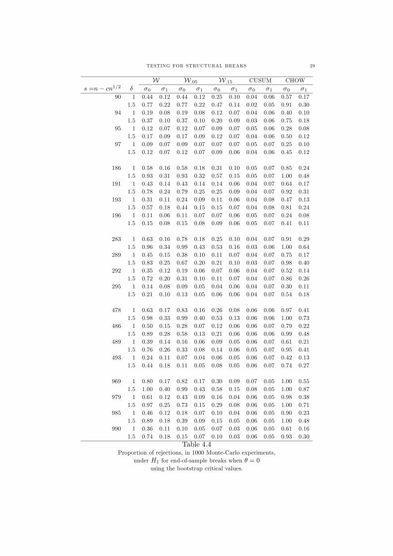
TESTING FOR STRUCTURAL BREAKS 29
W W:05 W:15 CUSUM CHOWs =n� cn1=2 � �0 �1 �0 �1 �0 �1 �0 �1 �0 �1
90 1 0.44 0.12 0.44 0.12 0.25 0.10 0.04 0.06 0.57 0.171.5 0.77 0.22 0.77 0.22 0.47 0.14 0.02 0.05 0.91 0.30
94 1 0.19 0.08 0.19 0.08 0.12 0.07 0.04 0.06 0.40 0.101.5 0.37 0.10 0.37 0.10 0.20 0.09 0.03 0.06 0.75 0.18
95 1 0.12 0.07 0.12 0.07 0.09 0.07 0.05 0.06 0.28 0.081.5 0.17 0.09 0.17 0.09 0.12 0.07 0.04 0.06 0.50 0.12
97 1 0.09 0.07 0.09 0.07 0.07 0.07 0.05 0.07 0.25 0.101.5 0.12 0.07 0.12 0.07 0.09 0.06 0.04 0.06 0.45 0.12
186 1 0.58 0.16 0.58 0.18 0.31 0.10 0.05 0.07 0.85 0.241.5 0.93 0.31 0.93 0.32 0.57 0.15 0.05 0.07 1.00 0.48
191 1 0.43 0.14 0.43 0.14 0.14 0.06 0.04 0.07 0.64 0.171.5 0.78 0.24 0.79 0.25 0.25 0.09 0.04 0.07 0.92 0.31
193 1 0.31 0.11 0.24 0.09 0.11 0.06 0.04 0.08 0.47 0.131.5 0.57 0.18 0.44 0.15 0.15 0.07 0.04 0.08 0.81 0.24
196 1 0.11 0.06 0.11 0.07 0.07 0.06 0.05 0.07 0.24 0.081.5 0.15 0.08 0.15 0.08 0.09 0.06 0.05 0.07 0.41 0.11
283 1 0.63 0.16 0.78 0.18 0.25 0.10 0.04 0.07 0.91 0.291.5 0.96 0.34 0.99 0.43 0.53 0.16 0.03 0.06 1.00 0.64
289 1 0.45 0.15 0.38 0.10 0.11 0.07 0.04 0.07 0.75 0.171.5 0.83 0.25 0.67 0.20 0.21 0.10 0.03 0.07 0.98 0.40
292 1 0.35 0.12 0.19 0.06 0.07 0.06 0.04 0.07 0.52 0.141.5 0.72 0.20 0.31 0.10 0.11 0.07 0.04 0.07 0.86 0.26
295 1 0.14 0.08 0.09 0.05 0.04 0.06 0.04 0.07 0.30 0.111.5 0.21 0.10 0.13 0.05 0.06 0.06 0.04 0.07 0.54 0.18
478 1 0.63 0.17 0.83 0.16 0.26 0.08 0.06 0.06 0.97 0.411.5 0.98 0.33 0.99 0.40 0.53 0.13 0.06 0.06 1.00 0.73
486 1 0.50 0.15 0.28 0.07 0.12 0.06 0.06 0.07 0.79 0.221.5 0.89 0.28 0.58 0.13 0.21 0.06 0.06 0.06 0.99 0.48
489 1 0.39 0.14 0.16 0.06 0.09 0.05 0.06 0.07 0.61 0.211.5 0.76 0.26 0.33 0.08 0.14 0.06 0.05 0.07 0.95 0.41
493 1 0.24 0.11 0.07 0.04 0.06 0.05 0.06 0.07 0.42 0.131.5 0.44 0.18 0.11 0.05 0.08 0.05 0.06 0.07 0.74 0.27
969 1 0.80 0.17 0.82 0.17 0.30 0.09 0.07 0.05 1.00 0.551.5 1.00 0.40 0.99 0.43 0.58 0.15 0.08 0.05 1.00 0.87
979 1 0.61 0.12 0.43 0.09 0.16 0.04 0.06 0.05 0.98 0.381.5 0.97 0.25 0.73 0.15 0.29 0.08 0.06 0.05 1.00 0.71
985 1 0.46 0.12 0.18 0.07 0.10 0.04 0.06 0.05 0.90 0.231.5 0.89 0.18 0.39 0.09 0.15 0.05 0.06 0.05 1.00 0.48
990 1 0.36 0.11 0.10 0.05 0.07 0.03 0.06 0.05 0.61 0.161.5 0.74 0.18 0.15 0.07 0.10 0.03 0.06 0.05 0.93 0.30
Table 4.4Proportion of rejections, in 1000 Monte-Carlo experiments,
under H1 for end-of-sample breaks when � = 0using the bootstrap critical values.

30 JAVIER HIDALGO AND MYUNG HWAN SEO
W W:05 W:15 CUSUM CHOWs =n� cn1=2 � �0 �1 �0 �1 �0 �1 �0 �1 �0 �1
90 1 0.39 0.11 0.39 0.11 0.19 0.09 0.04 0.06 0.56 0.131.5 0.74 0.20 0.74 0.20 0.29 0.11 0.03 0.05 0.88 0.26
94 1 0.21 0.08 0.21 0.08 0.14 0.07 0.04 0.06 0.41 0.101.5 0.30 0.11 0.30 0.11 0.18 0.09 0.03 0.06 0.73 0.20
95 1 0.11 0.08 0.11 0.08 0.10 0.06 0.05 0.07 0.25 0.061.5 0.14 0.09 0.14 0.09 0.11 0.07 0.04 0.06 0.46 0.11
97 1 0.08 0.06 0.08 0.06 0.08 0.06 0.05 0.07 0.20 0.071.5 0.08 0.06 0.08 0.06 0.09 0.05 0.04 0.07 0.43 0.10
186 1 0.54 0.17 0.56 0.18 0.30 0.11 0.04 0.07 0.85 0.241.5 0.90 0.28 0.92 0.34 0.49 0.17 0.04 0.07 1.00 0.46
191 1 0.37 0.13 0.38 0.15 0.13 0.07 0.04 0.07 0.57 0.191.5 0.70 0.21 0.71 0.24 0.19 0.07 0.04 0.07 0.89 0.29
193 1 0.18 0.10 0.20 0.10 0.10 0.06 0.04 0.08 0.44 0.141.5 0.27 0.12 0.28 0.14 0.13 0.08 0.04 0.07 0.75 0.24
196 1 0.10 0.08 0.11 0.08 0.07 0.06 0.04 0.07 0.20 0.071.5 0.11 0.08 0.11 0.09 0.10 0.07 0.04 0.07 0.38 0.12
283 1 0.55 0.14 0.69 0.17 0.21 0.09 0.04 0.07 0.86 0.281.5 0.90 0.31 0.96 0.38 0.36 0.14 0.03 0.07 1.00 0.60
289 1 0.39 0.12 0.25 0.08 0.10 0.06 0.04 0.07 0.67 0.171.5 0.74 0.22 0.42 0.15 0.15 0.07 0.03 0.07 0.96 0.35
292 1 0.34 0.11 0.15 0.06 0.06 0.06 0.04 0.07 0.52 0.121.5 0.67 0.19 0.24 0.09 0.09 0.06 0.03 0.07 0.82 0.22
295 1 0.09 0.06 0.07 0.05 0.05 0.05 0.04 0.07 0.29 0.091.5 0.09 0.07 0.07 0.05 0.05 0.06 0.04 0.07 0.48 0.15
478 1 0.63 0.17 0.78 0.16 0.24 0.07 0.06 0.06 0.97 0.371.5 0.96 0.34 0.98 0.39 0.44 0.12 0.05 0.06 1.00 0.68
486 1 0.46 0.16 0.27 0.07 0.11 0.05 0.06 0.07 0.76 0.211.5 0.84 0.27 0.45 0.12 0.17 0.06 0.05 0.06 0.99 0.45
489 1 0.37 0.15 0.14 0.05 0.08 0.04 0.06 0.07 0.56 0.211.5 0.71 0.23 0.20 0.07 0.10 0.05 0.05 0.06 0.91 0.36
493 1 0.15 0.11 0.06 0.05 0.05 0.05 0.06 0.07 0.40 0.161.5 0.19 0.14 0.07 0.05 0.07 0.05 0.05 0.07 0.69 0.25
969 1 0.75 0.17 0.73 0.18 0.25 0.07 0.06 0.05 1.00 0.511.5 0.99 0.38 0.95 0.39 0.47 0.13 0.06 0.05 1.00 0.86
979 1 0.57 0.13 0.33 0.10 0.14 0.05 0.06 0.05 0.98 0.391.5 0.94 0.29 0.57 0.17 0.23 0.07 0.06 0.05 1.00 0.68
985 1 0.45 0.12 0.16 0.06 0.09 0.05 0.06 0.05 0.87 0.251.5 0.82 0.20 0.26 0.09 0.14 0.06 0.06 0.05 0.99 0.49
990 1 0.37 0.12 0.10 0.05 0.07 0.04 0.06 0.05 0.64 0.171.5 0.71 0.17 0.13 0.07 0.10 0.05 0.06 0.05 0.92 0.36
Table 4.4 (continuation)Proportion of rejections, in 1000 Monte-Carlo experiments,
under H1 for end-of-sample breaks when � = �=4using the bootstrap critical values.

TESTING FOR STRUCTURAL BREAKS 31
W W:05 W:15 CUSUM CHOWs =n� cn1=2 � �0 �1 �0 �1 �0 �1 �0 �1 �0 �1
90 1 0.47 0.12 0.47 0.12 0.27 0.08 0.04 0.07 0.60 0.161.5 0.81 0.24 0.81 0.24 0.47 0.14 0.02 0.06 0.92 0.30
94 1 0.20 0.09 0.20 0.09 0.14 0.07 0.05 0.07 0.42 0.101.5 0.35 0.13 0.35 0.13 0.23 0.09 0.04 0.06 0.75 0.21
95 1 0.11 0.07 0.11 0.07 0.10 0.06 0.05 0.07 0.27 0.071.5 0.16 0.09 0.16 0.09 0.12 0.07 0.04 0.07 0.52 0.09
97 1 0.09 0.06 0.09 0.06 0.09 0.06 0.05 0.07 0.22 0.081.5 0.12 0.07 0.12 0.07 0.09 0.06 0.04 0.07 0.44 0.10
186 1 0.57 0.14 0.56 0.17 0.31 0.10 0.05 0.07 0.86 0.221.5 0.93 0.32 0.93 0.34 0.58 0.14 0.04 0.06 1.00 0.47
191 1 0.44 0.14 0.42 0.15 0.14 0.07 0.05 0.07 0.60 0.191.5 0.78 0.23 0.77 0.24 0.24 0.08 0.04 0.07 0.93 0.34
193 1 0.32 0.12 0.23 0.10 0.11 0.06 0.05 0.07 0.47 0.151.5 0.57 0.18 0.40 0.14 0.16 0.06 0.04 0.07 0.80 0.26
196 1 0.11 0.08 0.10 0.08 0.07 0.06 0.05 0.07 0.20 0.091.5 0.14 0.08 0.13 0.08 0.08 0.07 0.04 0.07 0.41 0.12
283 1 0.57 0.13 0.73 0.17 0.24 0.09 0.03 0.07 0.89 0.261.5 0.95 0.31 0.99 0.35 0.49 0.14 0.03 0.06 1.00 0.56
289 1 0.46 0.12 0.34 0.08 0.11 0.05 0.04 0.07 0.70 0.171.5 0.84 0.21 0.68 0.18 0.20 0.08 0.03 0.07 0.97 0.33
292 1 0.36 0.10 0.15 0.06 0.07 0.05 0.04 0.07 0.50 0.121.5 0.71 0.18 0.31 0.09 0.12 0.06 0.04 0.07 0.85 0.23
295 1 0.14 0.07 0.08 0.05 0.06 0.05 0.04 0.07 0.29 0.091.5 0.21 0.09 0.10 0.05 0.06 0.05 0.04 0.07 0.57 0.15
478 1 0.63 0.17 0.81 0.18 0.26 0.08 0.06 0.06 0.97 0.381.5 0.98 0.33 0.99 0.41 0.52 0.11 0.05 0.06 1.00 0.70
486 1 0.48 0.13 0.29 0.08 0.12 0.06 0.06 0.07 0.79 0.211.5 0.86 0.28 0.58 0.14 0.21 0.07 0.05 0.06 0.99 0.45
489 1 0.39 0.12 0.16 0.07 0.08 0.06 0.06 0.07 0.58 0.201.5 0.79 0.22 0.33 0.10 0.13 0.07 0.06 0.06 0.94 0.40
493 1 0.23 0.11 0.09 0.05 0.06 0.05 0.06 0.07 0.40 0.141.5 0.46 0.17 0.14 0.07 0.07 0.06 0.06 0.07 0.74 0.24
969 1 0.81 0.18 0.80 0.21 0.30 0.08 0.05 0.05 1.00 0.561.5 1.00 0.41 0.99 0.43 0.60 0.13 0.05 0.04 1.00 0.88
979 1 0.63 0.16 0.40 0.11 0.16 0.05 0.06 0.05 0.98 0.391.5 0.97 0.28 0.73 0.21 0.29 0.07 0.06 0.04 1.00 0.75
985 1 0.50 0.14 0.21 0.07 0.10 0.05 0.06 0.05 0.90 0.241.5 0.90 0.21 0.37 0.11 0.17 0.06 0.05 0.05 1.00 0.54
990 1 0.39 0.13 0.12 0.05 0.07 0.05 0.06 0.05 0.65 0.181.5 0.76 0.22 0.18 0.07 0.09 0.05 0.06 0.05 0.95 0.35
Table 4.4 (continuation)Proportion of rejections, in 1000 Monte-Carlo experiments,
under H1 for end-of-sample breaks when � = �=2using the bootstrap critical values.

32 JAVIER HIDALGO AND MYUNG HWAN SEO
London School of Economics, Houghton Street, London WC2A 2AE, UKE-mail address : [email protected]
London School of Economics, Houghton Street, London WC2A 2AE, UKE-mail address : [email protected]
Related Documents