Testing for directional symmetry in spatial dependence using the periodogram

Testing for Directional Symmetry in Spatial Dependence

Using the Periodogram

Nelson Lu1 Dale L. Zimmerman2

1Nelson Lu is Biostatistician, Wyeth Research, Pearl River, NY 10965 (E-mail: [email protected])

2Dale L. Zimmerman is Professor, Department of Statistics and Actuarial Science, University

of Iowa, Iowa City, IA 52242 (E-mail: [email protected]; Phone: 319-335-0818; Fax: 319-

335-3017). Please address all correspondence to this author.

Abstract

The characterization of spatial dependence is an important component of a spatial modeling

exercise. For reasons of convenience, model parsimony, or computational efficiency, the spa-

tial covariance structure is often assumed to be isotropic (direction-invariant), completely

symmetric, or reflection symmetric (the latter two being forms of directional invariance some-

what weaker than isotropy). We propose some diagnostic tests of the latter two properties

that are based on the two-dimensional periodogram. An advantage of basing tests on the

periodogram rather than the sample semivariogram or covariance function is that the pe-

riodogram ordinates corresponding to different frequencies are asymptotically independent,

leading to simpler distribution theory. A simulation study and two examples illustrate the

usefulness and limitations of the proposed tests.

1 Introduction

For spatial and spatio-temporal data, characterization of the covariance structure is an im-

portant component of a modeling exercise. For reasons of convenience, model parsimony,

and computational efficiency, the covariance structure often is assumed to have some type

of directional invariance property. For a two-dimensional, second-order stationary random

process defined on a square lattice, three important directional invariance properties are re-

flection symmetry, complete symmetry, and isotropy, defined as follows. In these definitions

C(j, k) denotes the covariance between two random variables lagged j columns and k rows

apart in the lattice.

Definition. A second-order stationary random process on a square lattice is said to be

reflection symmetric if its covariance function satisfies

C(j, k) = C(−j, k) for all (j, k) ∈ Z2.

Definition. A second-order stationary random process on a square lattice is said to be

completely symmetric if its covariance function satisfies

C(j, k) = C(−j, k) = C(k, j) = C(−k, j) for all (j, k) ∈ Z2.

Definition. A second-order stationary random process on a square lattice is said to be

isotropic if its covariance function satisfies

C(j, k) = C0(√

j2 + k2) for all (j, k) ∈ Z2,

where C0(·) is the covariance function of a one-dimensional random process.

The usage of these terms is quite widespread, though not universal: Gneiting (2002), for

example, refers to a spatio-temporal version of reflection symmetry as “full symmetry.” Note

1

that isotropy implies complete symmetry, which in turn implies reflection symmetry, but the

converses are not true.

In spatial analyses in which the dependence is assumed to satisfy a directional symmetry

property, diagnostic checking for the validity of the assumption has been spotty. At best,

the checking may be done informally through such graphical diagnostics as direction-specific

sample semivariogram plots and the rose diagram (Isaaks and Srivastava, 1989, pp. 149-154)

or via a qualitative comparison of the estimates of C(j, k) to those of C(−j, k), (j, k) ∈ Z2

(Modjeska and Rawlings, 1983). At worst, the assumption is simply not checked at all.

There is a real need for diagnostics that can be accompanied by formal testing. A step in

this direction was taken by Lu (1994), who developed a method for formally testing for any

directional symmetry hypothesis that can be expressed as linear equality constraints on the

covariance function or semivariogram (as can all three types of symmetry defined above).

Lu’s approach was based on a statistic that measured how well the sample covariance function

(or semivariogram) satisfied these linear equality constraints.

In this paper, we propose tests for reflection symmetry and complete symmetry that

are based on certain ratios of periodogram ordinates. An advantage of basing tests on the

periodogram rather than the sample covariance function or semivariogram is that the pe-

riodogram ordinates corresponding to different frequencies are asymptotically independent,

leading to simpler distribution theory and simpler implementation of the tests. There is a

long history of using the periodogram of one-dimensional processes to construct tests for pe-

riodicity, independence, and other properties; see, for example, Fisher (1929), Durbin (1967),

and Priestley and Rao (1969). The approach taken in the present article is very similar in

spirit to that of these earlier authors.

Consideration of directionally symmetric covariance structures plays a role in both spatial

analysis and design. In spatial experimental design, for example, Modjeska and Rawlings

(1983) determined the optimal plot size and shape for field-plot experiments under a two-

2

dimensional extension of Smith’s (1938) empirical model relating soil heterogeneity to plot

size and shape, and showed that this two-dimensional model implied a reflection symmetric

correlation structure. Martin and Eccleston (1993) developed spatial experimental designs

that are optimal under reflection symmetry or complete symmetry.

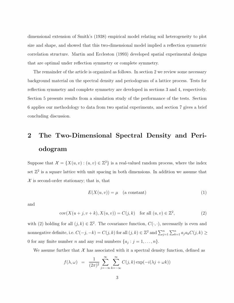
The remainder of the article is organized as follows. In section 2 we review some necessary

background material on the spectral density and periodogram of a lattice process. Tests for

reflection symmetry and complete symmetry are developed in sections 3 and 4, respectively.

Section 5 presents results from a simulation study of the performance of the tests. Section

6 applies our methodology to data from two spatial experiments, and section 7 gives a brief

concluding discussion.

2 The Two-Dimensional Spectral Density and Peri-

odogram

Suppose that X = {X(u, v) : (u, v) ∈ Z2} is a real-valued random process, where the index

set Z2 is a square lattice with unit spacing in both dimensions. In addition we assume that

X is second-order stationary; that is, that

E(X(u, v)) = µ (a constant) (1)

and

cov(X(u + j, v + k), X(u, v)) = C(j, k) for all (u, v) ∈ Z2, (2)

with (2) holding for all (j, k) ∈ Z2. The covariance function, C(·, ·), necessarily is even and

nonnegative definite, i.e. C(−j,−k) = C(j, k) for all (j, k) ∈ Z2 and

∑nj=1

∑nk=1 ajakC(j, k) ≥

0 for any finite number n and any real numbers {aj : j = 1, . . . , n}.

We assume further that X has associated with it a spectral density function, defined as

f(λ, ω) =1

(2π)2

∞∑

j=−∞

∞∑

k=−∞

C(j, k) exp(−i(λj + ωk))

3

=1

(2π)2

∞∑

j=−∞

∞∑

k=−∞

C(j, k) cos(λj + ωk) (3)

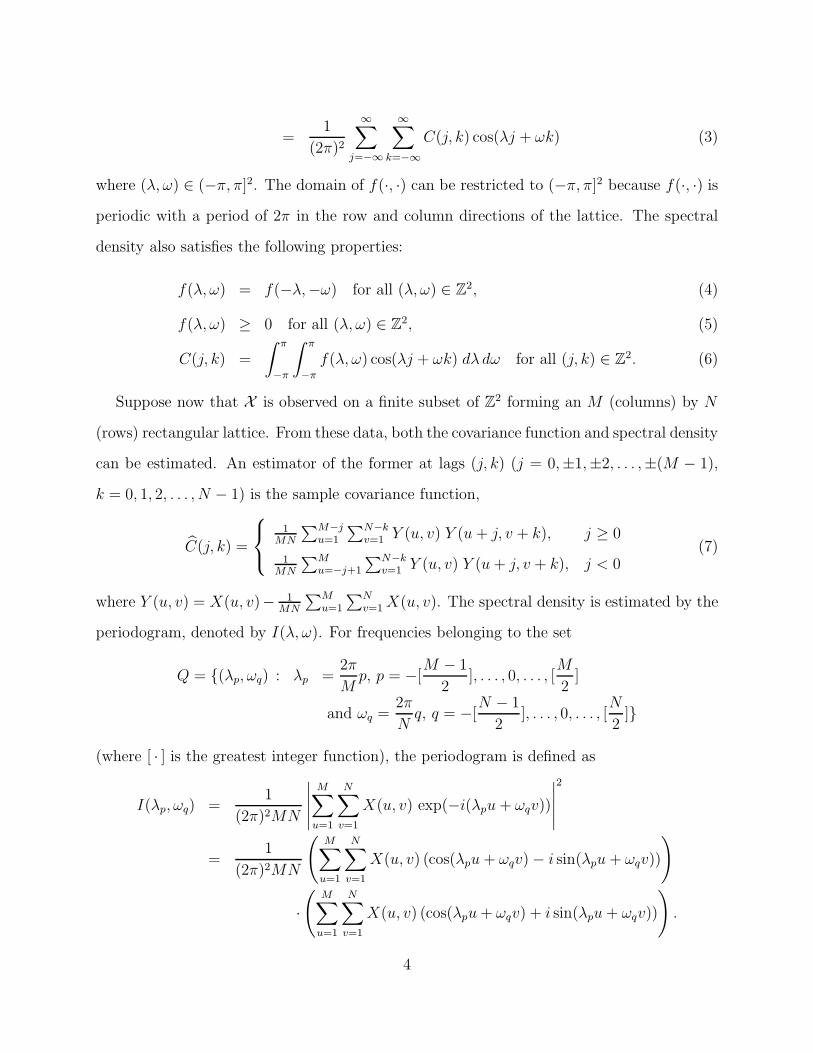
where (λ, ω) ∈ (−π, π]2. The domain of f(·, ·) can be restricted to (−π, π]2 because f(·, ·) is

periodic with a period of 2π in the row and column directions of the lattice. The spectral

density also satisfies the following properties:

f(λ, ω) = f(−λ,−ω) for all (λ, ω) ∈ Z2, (4)

f(λ, ω) ≥ 0 for all (λ, ω) ∈ Z2, (5)

C(j, k) =

∫ π

−π

∫ π

−π

f(λ, ω) cos(λj + ωk) dλ dω for all (j, k) ∈ Z2. (6)

Suppose now that X is observed on a finite subset of Z2 forming an M (columns) by N

(rows) rectangular lattice. From these data, both the covariance function and spectral density

can be estimated. An estimator of the former at lags (j, k) (j = 0,±1,±2, . . . ,±(M − 1),

k = 0, 1, 2, . . . , N − 1) is the sample covariance function,

C(j, k) =

1MN

∑M−ju=1

∑N−kv=1 Y (u, v) Y (u + j, v + k), j ≥ 0

1MN

∑Mu=−j+1

∑N−kv=1 Y (u, v) Y (u + j, v + k), j < 0

(7)

where Y (u, v) = X(u, v)− 1MN

∑Mu=1

∑Nv=1 X(u, v). The spectral density is estimated by the

periodogram, denoted by I(λ, ω). For frequencies belonging to the set

Q = {(λp, ωq) : λp =2π

Mp, p = −[

M − 1

2], . . . , 0, . . . , [

M

2]

and ωq =2π

Nq, q = −[

N − 1

2], . . . , 0, . . . , [

N

2]}

(where [ · ] is the greatest integer function), the periodogram is defined as

I(λp, ωq) =1

(2π)2MN

∣∣∣∣∣

M∑

u=1

N∑

v=1

X(u, v) exp(−i(λpu + ωqv))

∣∣∣∣∣

2

=1

(2π)2MN

(M∑

u=1

N∑

v=1

X(u, v) (cos(λpu + ωqv) − i sin(λpu + ωqv))

)

·

(M∑

u=1

N∑

v=1

X(u, v) (cos(λpu + ωqv) + i sin(λpu + ωqv))

).

4

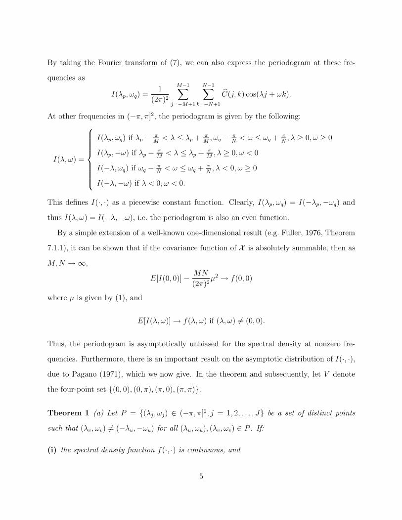
By taking the Fourier transform of (7), we can also express the periodogram at these fre-

quencies as

I(λp, ωq) =1

(2π)2

M−1∑

j=−M+1

N−1∑

k=−N+1

C(j, k) cos(λj + ωk).

At other frequencies in (−π, π]2, the periodogram is given by the following:

I(λ, ω) =

I(λp, ωq) if λp −πM

< λ ≤ λp + πM

, ωq −πN

< ω ≤ ωq + πN

, λ ≥ 0, ω ≥ 0

I(λp,−ω) if λp −πM

< λ ≤ λp + πM

, λ ≥ 0, ω < 0

I(−λ, ωq) if ωq −πN

< ω ≤ ωq + πN

, λ < 0, ω ≥ 0

I(−λ,−ω) if λ < 0, ω < 0.

This defines I(·, ·) as a piecewise constant function. Clearly, I(λp, ωq) = I(−λp,−ωq) and

thus I(λ, ω) = I(−λ,−ω), i.e. the periodogram is also an even function.

By a simple extension of a well-known one-dimensional result (e.g. Fuller, 1976, Theorem

7.1.1), it can be shown that if the covariance function of X is absolutely summable, then as

M, N → ∞,

E[I(0, 0)] −MN

(2π)2µ2 → f(0, 0)

where µ is given by (1), and

E[I(λ, ω)] → f(λ, ω) if (λ, ω) 6= (0, 0).

Thus, the periodogram is asymptotically unbiased for the spectral density at nonzero fre-

quencies. Furthermore, there is an important result on the asymptotic distribution of I(·, ·),

due to Pagano (1971), which we now give. In the theorem and subsequently, let V denote

the four-point set {(0, 0), (0, π), (π, 0), (π, π)}.

Theorem 1 (a) Let P = {(λj , ωj) ∈ (−π, π]2, j = 1, 2, . . . , J} be a set of distinct points

such that (λv, ωv) 6= (−λu,−ωu) for all (λu, ωu), (λv, ωv) ∈ P . If:

(i) the spectral density function f(·, ·) is continuous, and

5

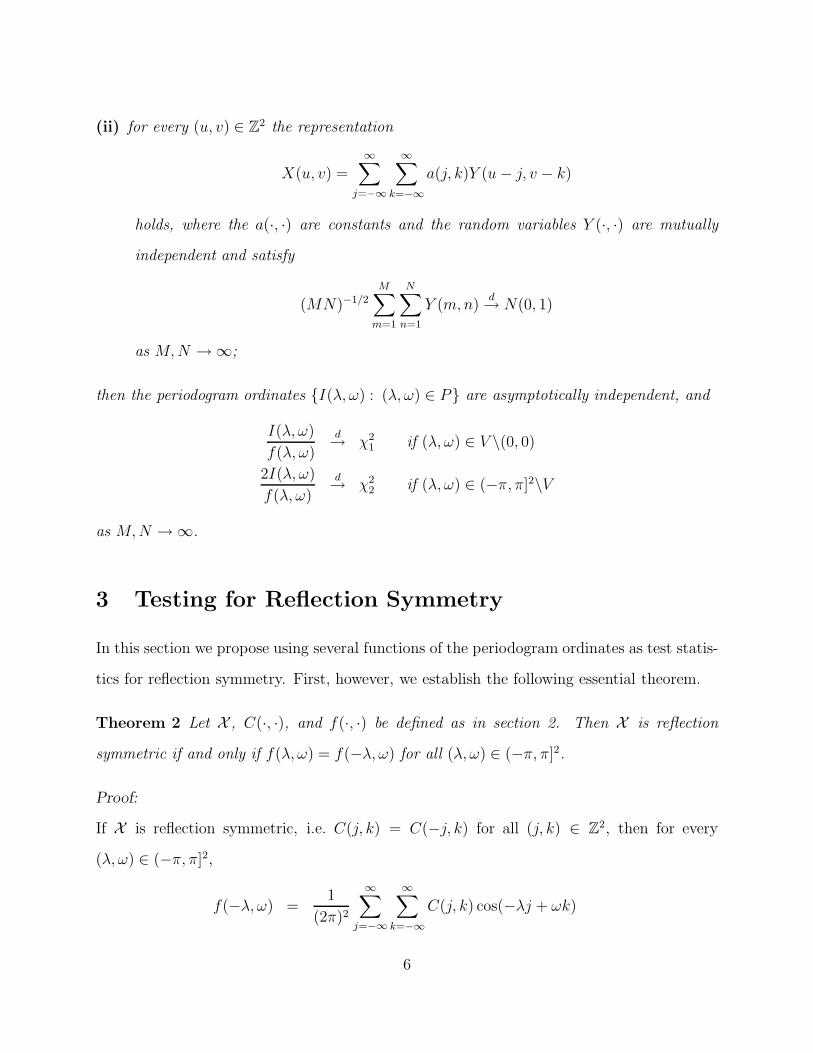
(ii) for every (u, v) ∈ Z2 the representation

X(u, v) =∞∑

j=−∞

∞∑

k=−∞

a(j, k)Y (u − j, v − k)

holds, where the a(·, ·) are constants and the random variables Y (·, ·) are mutually

independent and satisfy

(MN)−1/2

M∑

m=1

N∑

n=1

Y (m, n)d→ N(0, 1)

as M, N → ∞;

then the periodogram ordinates {I(λ, ω) : (λ, ω) ∈ P} are asymptotically independent, and

I(λ, ω)

f(λ, ω)

d→ χ2

1 if (λ, ω) ∈ V \(0, 0)

2I(λ, ω)

f(λ, ω)

d→ χ2

2 if (λ, ω) ∈ (−π, π]2\V

as M, N → ∞.

3 Testing for Reflection Symmetry

In this section we propose using several functions of the periodogram ordinates as test statis-

tics for reflection symmetry. First, however, we establish the following essential theorem.

Theorem 2 Let X , C(·, ·), and f(·, ·) be defined as in section 2. Then X is reflection

symmetric if and only if f(λ, ω) = f(−λ, ω) for all (λ, ω) ∈ (−π, π]2.

Proof:

If X is reflection symmetric, i.e. C(j, k) = C(−j, k) for all (j, k) ∈ Z2, then for every

(λ, ω) ∈ (−π, π]2,

f(−λ, ω) =1

(2π)2

∞∑

j=−∞

∞∑

k=−∞

C(j, k) cos(−λj + ωk)

6

=1

(2π)2

∞∑

j=−∞

∞∑

k=−∞

C(−j, k) cos(λ(−j) + ωk)

=1

(2π)2

∞∑

j=−∞

∞∑

k=−∞

C(j, k) cos(λj + ωk)

= f(λ, ω)

where we have used (3). Conversely, if f(λ, ω) = f(−λ, ω) for all (λ, ω) ∈ (−π, π]2, then for

all (j, k) ∈ Z2,

C(−j, k) =

∫ π

−π

∫ π

−π

f(λ, ω) cos(−jλ + kω) dλ dω

=

∫ π

−π

∫ π

−π

f(−λ, ω) cos(−jλ + kω) dλ dω

=

∫ π

−π

∫ π

−π

f(λ, ω) cos(jλ + kω) dλ dω

= C(j, k)

where we have used (6). Q.E.D.

Theorem 2 indicates that the hypothesis of reflection symmetry can be expressed as either

H0 : C(j, k) = C(−j, k) for all (j, k) ∈ Z2

or

H0 : f(λ, ω) = f(−λ, ω) for all (λ, ω) ∈ (−π, π]2.

We use the periodogram to test this second representation of H0 against the alternative

hypothesis HA: not H0.

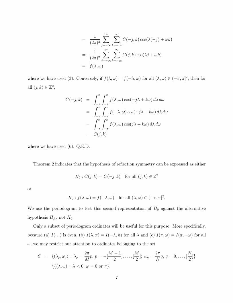
Only a subset of periodogram ordinates will be useful for this purpose. More specifically,

because (a) I(·, ·) is even, (b) I(λ, π) = I(−λ, π) for all λ and (c) I(π, ω) = I(π,−ω) for all

ω, we may restrict our attention to ordinates belonging to the set

S = {(λp, ωq) : λp =2π

Mp, p = −[

M − 1

2], . . . , [

M

2]; ωq =

2π

Nq, q = 0, . . . , [

N

2]}

\{(λ, ω) : λ < 0, ω = 0 or π}.

7

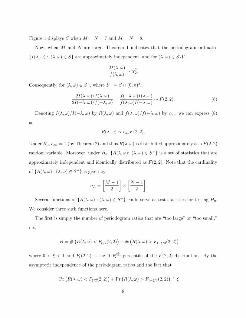
Figure 1 displays S when M = N = 7 and M = N = 8.

Now, when M and N are large, Theorem 1 indicates that the periodogram ordinates

{I(λ, ω) : (λ, ω) ∈ S} are approximately independent, and for (λ, ω) ∈ S\V ,

2I(λ, ω)

f(λ, ω)

·∼ χ2

2.

Consequently, for (λ, ω) ∈ S+, where S+ = S ∩ (0, π)2,

2I(λ, ω)/f(λ, ω)

2I(−λ, ω)/f(−λ, ω)=

f(−λ, ω)I(λ, ω)

f(λ, ω)I(−λ, ω)

·∼ F (2, 2). (8)

Denoting I(λ, ω)/I(−λ, ω) by R(λ, ω) and f(λ, ω)/f(−λ, ω) by cλω, we can express (8)

as

R(λ, ω)·∼ cλωF (2, 2).

Under H0, cλω = 1 (by Theorem 2) and thus R(λ, ω) is distributed approximately as a F (2, 2)

random variable. Moreover, under H0, {R(λ, ω): (λ, ω) ∈ S+} is a set of statistics that are

approximately independent and identically distributed as F (2, 2). Note that the cardinality

of {R(λ, ω) : (λ, ω) ∈ S+} is given by

nR =

[M − 1

2

]×

[N − 1

2

].

Several functions of {R(λ, ω) : (λ, ω) ∈ S+} could serve as test statistics for testing H0.

We consider three such functions here.

The first is simply the number of periodogram ratios that are “too large” or “too small,”

i.e.,

B = #(R(λ, ω) < Fξ/2(2, 2)

)+ #

(R(λ, ω) > F1−ξ/2(2, 2)

)

where 0 < ξ < 1 and Fξ(2, 2) is the 100ξth percentile of the F (2, 2) distribution. By the

asymptotic independence of the periodogram ratios and the fact that

Pr(R(λ, ω) < Fξ/2(2, 2)

)+ Pr

(R(λ, ω) > F1−ξ/2(2, 2)

) .= ξ

8

under H0 for all (λ, ω) ∈ S+, the asymptotic null distribution of B is binomial with sample

size parameter nR and success probability ξ, i.e., B·∼ bin(nR, ξ) under H0. Accordingly, an

approximately size-α test of H0 versus HA is to reject H0 if B > b, where b can be attained

by solving α = Pr(bin(nR, ξ) > b) for b.

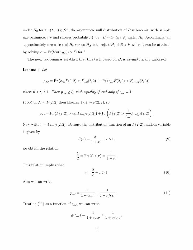
The next two lemmas establish that this test, based on B, is asymptotically unbiased.

Lemma 1 Let

pλω = Pr(cλωF (2, 2) < Fξ/2(2, 2)

)+ Pr

(cλωF (2, 2) > F1−ξ/2(2, 2)

)

where 0 < ξ < 1. Then pλω ≥ ξ, with equality if and only if cλω = 1.

Proof: If X ∼ F (2, 2) then likewise 1/X ∼ F (2, 2), so

pλω = Pr(F (2, 2) > cλωF1−ξ/2(2, 2)

)+ Pr

(F (2, 2) >

1

cλω

F1−ξ/2(2, 2)

).

Now write ν = F1−ξ/2(2, 2). Because the distribution function of an F (2, 2) random variable

is given by

F (x) =x

1 + x, x > 0, (9)

we obtain the relation

ξ

2= Pr(X > ν) =

1

1 + ν.

This relation implies that

ν =2

ǫ− 1 > 1. (10)

Also we can write

pλω =1

1 + cλων+

1

1 + ν/cλω. (11)

Treating (11) as a function of cλω, we can write

g(cλω) =1

1 + cλων+

1

1 + ν/cλω

,

9

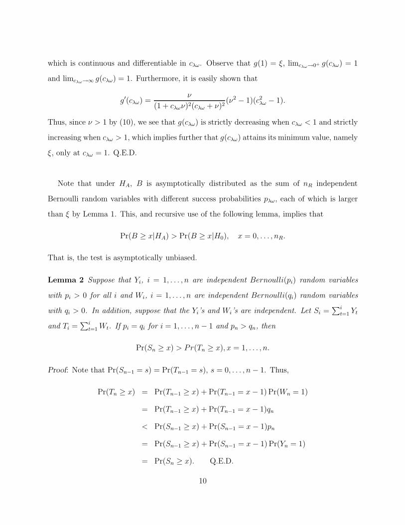
which is continuous and differentiable in cλω. Observe that g(1) = ξ, limcλω→0+ g(cλω) = 1

and limcλω→∞ g(cλω) = 1. Furthermore, it is easily shown that

g′(cλω) =ν

(1 + cλων)2(cλω + ν)2(ν2 − 1)(c2

λω − 1).

Thus, since ν > 1 by (10), we see that g(cλω) is strictly decreasing when cλω < 1 and strictly

increasing when cλω > 1, which implies further that g(cλω) attains its minimum value, namely

ξ, only at cλω = 1. Q.E.D.

Note that under HA, B is asymptotically distributed as the sum of nR independent

Bernoulli random variables with different success probabilities pλω, each of which is larger

than ξ by Lemma 1. This, and recursive use of the following lemma, implies that

Pr(B ≥ x|HA) > Pr(B ≥ x|H0), x = 0, . . . , nR.

That is, the test is asymptotically unbiased.

Lemma 2 Suppose that Yi, i = 1, . . . , n are independent Bernoulli(pi) random variables

with pi > 0 for all i and Wi, i = 1, . . . , n are independent Bernoulli(qi) random variables

with qi > 0. In addition, suppose that the Yi’s and Wi’s are independent. Let Si =∑i

t=1 Yt

and Ti =∑i

t=1 Wt. If pi = qi for i = 1, . . . , n − 1 and pn > qn, then

Pr(Sn ≥ x) > Pr(Tn ≥ x), x = 1, . . . , n.

Proof: Note that Pr(Sn−1 = s) = Pr(Tn−1 = s), s = 0, . . . , n − 1. Thus,

Pr(Tn ≥ x) = Pr(Tn−1 ≥ x) + Pr(Tn−1 = x − 1) Pr(Wn = 1)

= Pr(Tn−1 ≥ x) + Pr(Tn−1 = x − 1)qn

< Pr(Sn−1 ≥ x) + Pr(Sn−1 = x − 1)pn

= Pr(Sn−1 ≥ x) + Pr(Sn−1 = x − 1) Pr(Yn = 1)

= Pr(Sn ≥ x). Q.E.D.

10

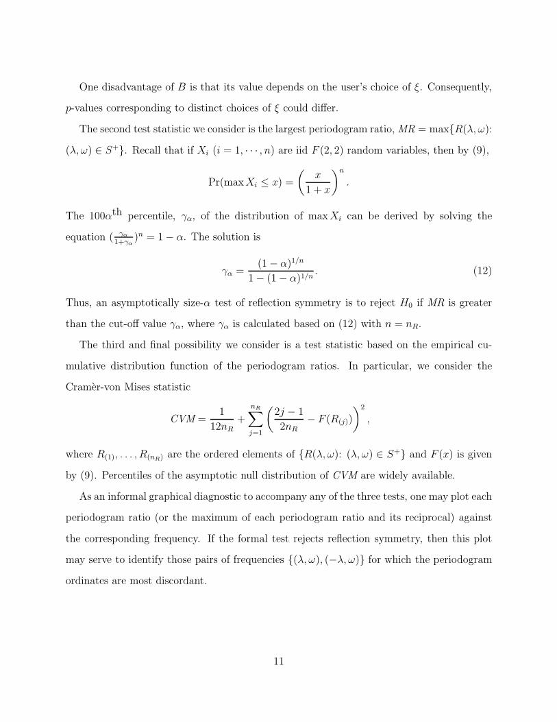
One disadvantage of B is that its value depends on the user’s choice of ξ. Consequently,

p-values corresponding to distinct choices of ξ could differ.

The second test statistic we consider is the largest periodogram ratio, MR = max{R(λ, ω):

(λ, ω) ∈ S+}. Recall that if Xi (i = 1, · · · , n) are iid F (2, 2) random variables, then by (9),

Pr(max Xi ≤ x) =

(x

1 + x

)n

.

The 100αth percentile, γα, of the distribution of maxXi can be derived by solving the

equation ( γα

1+γα)n = 1 − α. The solution is

γα =(1 − α)1/n

1 − (1 − α)1/n. (12)

Thus, an asymptotically size-α test of reflection symmetry is to reject H0 if MR is greater

than the cut-off value γα, where γα is calculated based on (12) with n = nR.

The third and final possibility we consider is a test statistic based on the empirical cu-

mulative distribution function of the periodogram ratios. In particular, we consider the

Cramer-von Mises statistic

CVM =1

12nR+

nR∑

j=1

(2j − 1

2nR− F (R(j))

)2

,

where R(1), . . . , R(nR) are the ordered elements of {R(λ, ω): (λ, ω) ∈ S+} and F (x) is given

by (9). Percentiles of the asymptotic null distribution of CVM are widely available.

As an informal graphical diagnostic to accompany any of the three tests, one may plot each

periodogram ratio (or the maximum of each periodogram ratio and its reciprocal) against

the corresponding frequency. If the formal test rejects reflection symmetry, then this plot

may serve to identify those pairs of frequencies {(λ, ω), (−λ, ω)} for which the periodogram

ordinates are most discordant.

11

4 Testing for Complete Symmetry

The following theorem is useful for developing a procedure for testing for complete symmetry.

It can be proved in a manner similar to the proof of Theorem 2.

Theorem 3 Let X , C(·, ·), and f(·, ·) be defined as in section 2. Then X is completely

symmetric if and only if f(λ, ω) = f(−λ, ω) = f(ω, λ) = f(−ω, λ) for all (λ, ω) ∈ (−π, π]2.

Since complete symmetry implies reflection symmetry, rejection of reflection symmetry

implies rejection of complete symmetry. However, if the hypothesis of reflection symmetry

is not rejected, further investigation of complete symmetry may proceed. In this event we

consider testing

H∗0 : f(λ, ω) = f(ω, λ) for all (λ, ω) ∈ (−π, π]2

against H∗A: not H∗

0 . Thus, we propose to test for complete symmetry by a two-stage process

of first testing for reflection symmetry, i.e. testing for H0 as it was defined in section 3, and

then testing for H∗0 . If desired, the Bonferroni method can be used to maintain a specified

overall significance level for this two-stage testing procedure. An approach for simultaneously

testing for H0 and H∗0 could be contemplated, but it is more difficult to carry out in practice

because consideration of the joint asymptotic distribution of two (dependent) periodogram

ratios is required to obtain cut-off points.

The procedures for testing H∗0 that we consider are very similar to procedures we have

previously described for testing for reflection symmetry. We illustrate for the case M = N

only.

Using Theorem 1 again, we have

2I(λ, ω)/f(λ, ω)

2I(ω, λ)/f(ω, λ)=

f(ω, λ)I(λ, ω)

f(λ, ω)I(ω, λ)

·∼ F (2, 2)

for (λ, ω) ∈ S\V . When M is even, we also have

I(π, 0)/f(π, 0)

I(0, π)/f(0, π)=

f(0, π)I(π, 0)

f(π, 0)I(0, π)

·∼ F (1, 1).

12

Denote I(λ, ω)/I(ω, λ) by R∗MN (λ, ω) and f(λ, ω)/f(ω, λ) by c∗λω, and define the set

T+ = (S ∩ [0, π]2) \ (0, 0).

The cardinality of T+ is different from that of S+ and is given by

n∗R =

(M−1

2

)2, if M is odd

(M2

)2− M

2+ 1, if M is even.

To see this, note that when M is odd, there are 1 + 2 + . . . + M−12

ratios of the form I(λ,ω)I(ω,λ)

where λ and ω are strictly positive, and 1 + 2 + . . . + M−32

ratios of the form I(λ,ω)I(ω,λ)

where

λ < 0 and ω > 0. When M is even, there are M2

ratios of the form I(λ,0)I(0,λ)

, 1+2+ . . .+(M2−1)

ratios of the form I(λ,ω)I(ω,λ)

where λ and ω are strictly positive, and 1 + 2 + . . . + (M2− 2) ratios

of the form I(λ,ω)I(ω,λ)

where λ < 0 and ω > 0.

Now let B∗ denote the number of periodogram ratios in T+ that are either “too large”

or “too small.” Using arguments similar to those given in Section 3, every p∗λω attains its

minimum ξ (where 0 < ξ < 1) if and only if H∗0 is true, where

p∗λω =

Pr(F (1, 1) > cλωF1−ξ/2(1, 1)

)+ Pr

(F (1, 1) > 1

cλω

F1−ξ/2(1, 1)), if (λ, ω) = (π, 0)

Pr(F (2, 2) > cλωF1−ξ/2(2, 2)

)+ Pr

(F (2, 2) > 1

cλω

F1−ξ/2(2, 2)), otherwise.

Since the periodogram ratios in T+ are asymptotically independent and converge in distri-

bution to F (2, 2) (with the exception of I(0,π)I(π,0)

when M is even, which converges to F (1, 1)),

B∗ is asymptotically distributed as bin(n∗R, ξ) under H∗

0 . The value b for which the rejection

region {B∗ : B∗ > b} corresponds to a test of approximate size α can be obtained by solving

α = Pr(bin(n∗R, ξ) > b) for b.

Tests for H∗0 based on the largest periodogram ratio, or on the empirical distribution

function of periodogram ratios, in T+ can be implemented similarly, the only difference

being that the ratio I(0, π)/I(π, 0) must be excluded from consideration.

13

5 Simulation Study

In this section we report results of a simulation study of the three tests for reflection sym-

metry described in section 3. Simulation results for the tests for complete symmetry are

qualitively similar, hence for the sake of brevity we do not include them.

We generated realizations of zero-mean, second-order stationary, Gaussian and contami-

nated Gaussian processes having three different covariance structures, on an M by M square

lattice with unit spacing. Four different lattice sizes were considered, corresponding to M

= 11, 15, 21, and 25. The three covariance structures were associated with exponential co-

variance functions having unit variance but different directional symmetry properties. The

covariance functions we considered were as follows:

C1(j, k) = exp{−0.1

√2j2 + 2k2

},

C2(j, k) = exp{−0.1

√5j2 − 6jk + 5k2

},

C3(j, k) = exp{−0.1

√17j2 − 30jk + 17k2

}.

Observe that C1 is reflection symmetric (in fact it is isotropic), but C2 and C3 are not. Figure

2 depicts the shape of isocorrelation contours (loci of constant correlation) corresponding to

the three functions. The isocorrelation contours of C1 are circular, while those of C2 and C3

are ellipses whose main axes are oriented at 45 and 135 degree angles from horizontal axis.

Moreover, the ratio of the longer principal axis to the shorter one for C2 is 2:1 while the

ratio for C3 is 4:1; hence C3 is more reflection asymmetric than C2.

For each Gaussian process X = {X(u, v): (u, v) ∈ Z2} that we included in our study, we

also considered a contaminated Gaussian process Y = {Y (u, v): (u, v) ∈ Z2}, given by

Y =

X with probability 1 − ǫ

W with probability ǫ,

where W = {W (u, v): (u, v) ∈ Z2} is a zero-mean Gaussian process, independent of X ,

satisfying cov(W (u, v), W (s, t)) = k2 · cov(X(u, v), X(s, t)) for all (u, v), (s, t) ∈ Z2, and

14

k2 > 1. In this model, which is a generalization of the additive outliers model of Fox (1972)

for a time series, ǫ measures the amount of contamination and k2 measures how much more

variable W is than X . Here, we chose ǫ = 0.05 and k2 = 9, which represent a moderate

amount of contamination and extra variability and are the same values that Hawkins and

Cressie (1984) used in a simulation study of different variogram estimators.

An important feature of this contaminated normal process is that if X is reflection sym-

metric, then so is Y . To see this, first observe that

Y (u, v) = X(u, v)1{U>ǫ} + W (u, v)1{U≤ǫ},

where 1A is the indicator function for the set A and U is a uniform (0,1) random variable,

independent of X and W. Accordingly,

cov(Y (u, v), Y (s, t)) = E(Y (u, v)Y (s, t))

= E{(X(u, v)1{U>ǫ} + W (u, v)1{U≤ǫ})(X(s, t)1{U>ǫ} + W (s, t)1{U≤ǫ})}

= E{X(u, v)X(s, t)1{U>ǫ}1{U>ǫ}} + E{W (u, v)W (s, t)1{U≤ǫ}1{U≤ǫ}}

= (1 − ǫ)2cov(X(u, v), X(s, t)) + ǫ2cov(W (u, v), W (s, t))

= {(1 − ǫ)2 + k2ǫ2}cov(X(u, v), X(s, t)).

Therefore, Y is reflection symmetric if and only if X is reflection symmetric.

Ten thousand realizations of M2 observations were generated from each of the six processes

we considered. For each realization, the periodogram was computed and used to carry out the

tests based on B, MR, and CVM. We report results for tests conducted at the 0.05 significance

level only; results corresponding to significance levels 0.01 and 0.10 were qualitatively similar.

For the test based on B, we chose ξ to be 0.2; for this choice the critical values corresponding

to M = 11, 15, 21, and 25 were b = 8, 14, 26, and 36, respectively.

Results of the simulation study are presented in Table 1. Some observations from these

results are as follows.

15

1. Most of the empirical sizes are close to the nominal size of 0.05. The size of the B-test

tends to be a bit too low, while that of the CVM-test tends to be a little high when

the process is contaminated Gaussian.

2. The power of the tests, as expected, increases sharply as the sample size increases and

as the degree of reflection asymmetry in the covariance function increases.

3. The CVM-test has much higher power than the other two tests, across all combinations

of sample size and process. The B-test is the next best, while the MR-test is virtually

powerless. It appears that basing a test on only the largest periodogram ratio ignores

too much information to be useful.

4. The tests as a whole perform considerably worse for the contaminated Gaussian data

than for the Gaussian data. Only the CVM-test retains acceptable levels of power

when the data are contaminated Gaussian.

Thus, the main practical conclusion we make is that the CVM-test is quite powerful, and

we recommend its general use as a test for reflection symmetry, especially when the sample

size is larger than 200 (100 if the data are Gaussian). We do not recommend the other two

tests.

6 Examples

In this section, we present two examples to illustrate the use of the CVM-test for reflection

symmetry with actual data.

The first dataset we consider was given by Mercer and Hall (1911) and has been used to

illustrate the fitting of lattice models by several authors. The data are yields of wheat grain

(in pounds) over 500 plots arranged in a 25-column by 20-row lattice covering approximately

one acre. Further description and analysis of the data can be found in Cressie (1991, pp. 248-

16

259 and 453-458). Cressie determined that a nonlinear trend exists within rows; accordingly

he detrended the data using median polish and based further analysis on the median-polish

residuals. We follow his lead and apply our CVM-test to residuals obtained from a median

polish of the data.

The second dataset we consider was reported by Batchelor and Reed (1918) and comes

from a uniformity trial on the growth of orange trees. The data are yields of fruit (in

pounds) from 240 Valencia orange trees planted approximately 20 feet apart and arranged

in a 12-column by 20-row lattice. We apply our test directly to these yields.

For the wheat data residuals, CVM = 0.033, and the corresponding p-value is 0.96. Thus,

there is no statistical evidence of reflection asymmetry in these data, and it is reasonable to

proceed with an analysis that assumes reflection symmetry.

For the orange data, however, CVM = 0.395, with a p-value of 0.07. This suggests that

reflection symmetry may be somewhat tenuous for these data. Indeed, the sample covariance

function for the orange data (not shown) reveals a preponderance of small (less than 0.2 in

modulus) negative correlations among responses lagged five to ten units apart in a “NW-

SE” orientation, whereas there were approximately equal numbers of positive and negative

correlations among responses lagged five to ten units apart in a “NE-SW” orientation. We

believe it would be unwise to adopt a reflection symmetric model for further analysis of these

data.

7 Discussion

We have developed several tests for reflection symmetry and complete symmetry that are

based on ratios of certain periodogram ordinates. Of the tests we considered, the Cramer-von

Mises test, which compares the empirical distribution function of periodogram ratios to their

asymptotic null distribution function, emerged as the test with the fewest practical limita-

tions and highest power. Subject to some modest sample size requirements, we recommend

17

that it be used routinely as a diagnostic test for these directional symmetry properties.

It would be natural to consider using a similar approach to test for isotropy. Unlike

reflection and complete symmetry, however, isotropy cannot be fully characterized by a

set of simple symmetry conditions on the spectral density function. Note that isotropy

requires not only that C(j, k) = C(−j, k) = C(k, j) = C(k,−j) for all lags (and hence that

f(λ, ω) = f(−λ, ω) = f(ω, λ) = f(−ω, λ) for all frequencies) but also such conditions as

C(3, 4) = C(5, 0), C(5, 12) = C(13, 0), etc., which do not translate into simple conditions on

f(·, ·).

Throughout this article we allowed the number of rows and the number of columns in the

lattice of observation sites to be different, but we assumed that the spacing within rows was

equal to the spacing within columns. It is worth noting that our approach for testing for

reflection symmetry can also be applied to situations where the spacing is different within

rows than within columns. Testing for complete symmetry, however, requires equal spacing

within rows and columns, as otherwise it is not meaningful to compare estimates of f(λ, ω)

to estimates of f(ω, λ).

REFERENCES

Batchelor, L.D. and Reed, H.S. (1918). Relation of the variability of yields of fruit trees

to the accuracy of field trials. Journal of Agricultural Research, 12, 245-283.

Cressie, N.A.C. (1993). Statistics for Spatial Data, revised ed., New York: Wiley.

Durbin, J. (1967). Tests of serial independence based on the cumulated periodogram.

Bulletin of the International Statistics Institute, 42, 1039-1049.

Fisher, R.A. (1929). Tests of significance in harmonic analysis. Proceedings of the Royal

Society of London, Series A, 125, 54-59.

Fox, A.J. (1972). Outliers in time series. Journal of the Royal Statistical Society, Series

B, 34, 350-363.

18

Fuller, W.A. (1976). Introduction to Statistical Time Series. New York: John Wiley.

Gneiting, T. (2002). Nonseparable, stationary covariance functions for space-time data.

Journal of the American Statistical Association, 97, 590-600.

Hawkins, D.M. and Cressie, N. (1984). Robust kriging — a proposal. Journal of the

International Association for Mathematical Geology, 16, 3-18.

Isaaks, E.H. and Srivastava, R.M. (1989). Applied Geostatistics. New York: Oxford

University Press.

Lu, Hsiao-Chuan (1994). On the Distributions of the Sample Covariogram and Semivar-

iogram and Their Use in Testing for Isotropy, Ph.D. Thesis, University of Iowa.

Martin, R.J. and Eccleston, J.A. (1993). Incomplete block designs with spatial layouts

when observations are dependent. Journal of Statistical Planning and Inference, 35,

77-91.

Mercer, W.B. and Hall, A.D. (1911). The experimental error of field trials. Journal of

Agricultural Science (Cambridge), 4, 107-132.

Modjeska, J.S. and Rawlings, J.O. (1983). Spatial correlation analysis of uniformity data.

Biometrics, 39, 373-384.

Pagano, M. (1971). Some asymptotic properties of a two-dimensional periodogram, Jour-

nal of Applied Probability, 8, 841-847.

Priestley, M.B. and Rao, T.S. (1969). A test for non-stationarity of time-series. Journal

of the Royal Statistical Society Series B, 31, 140-149.

Smith, H.F. (1938). An empirical law describing heterogenity in the yields of agricultural

crops. Journal of Agricultural Science, 28, 1-23.

19

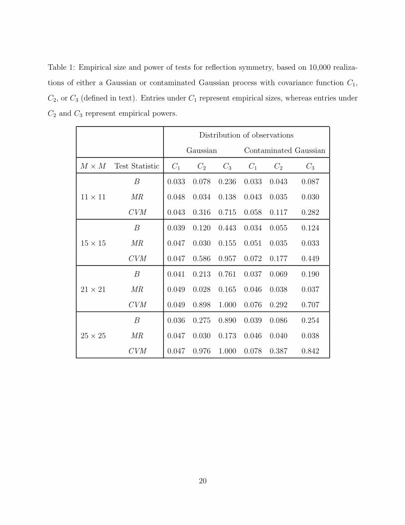
Table 1: Empirical size and power of tests for reflection symmetry, based on 10,000 realiza-

tions of either a Gaussian or contaminated Gaussian process with covariance function C1,

C2, or C3 (defined in text). Entries under C1 represent empirical sizes, whereas entries under

C2 and C3 represent empirical powers.

Distribution of observations

Gaussian Contaminated Gaussian

M × M Test Statistic C1 C2 C3 C1 C2 C3

B 0.033 0.078 0.236 0.033 0.043 0.087

11 × 11 MR 0.048 0.034 0.138 0.043 0.035 0.030

CVM 0.043 0.316 0.715 0.058 0.117 0.282

B 0.039 0.120 0.443 0.034 0.055 0.124

15 × 15 MR 0.047 0.030 0.155 0.051 0.035 0.033

CVM 0.047 0.586 0.957 0.072 0.177 0.449

B 0.041 0.213 0.761 0.037 0.069 0.190

21 × 21 MR 0.049 0.028 0.165 0.046 0.038 0.037

CVM 0.049 0.898 1.000 0.076 0.292 0.707

B 0.036 0.275 0.890 0.039 0.086 0.254

25 × 25 MR 0.047 0.030 0.173 0.046 0.040 0.038

CVM 0.047 0.976 1.000 0.078 0.387 0.842

20

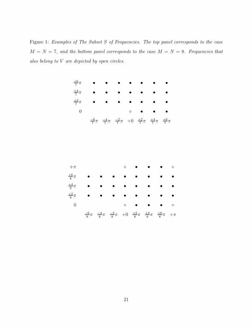
Figure 1: Examples of The Subset S of Frequencies. The top panel corresponds to the case

M = N = 7, and the bottom panel corresponds to the case M = N = 8. Frequencies that

also belong to V are depicted by open circles.

+67

π • • • • • • •

+47

π • • • • • • •

+27

π • • • • • • •

0 ◦ • • •

−67

π −47

π −27

π +0 +27

π +47

π +67

π

+π ◦ • • • ◦

+68

π • • • • • • • •

+48

π • • • • • • • •

+28

π • • • • • • • •

0 ◦ • • • ◦

−68

π −48

π −28

π +0 +28

π +48

π +68

π +π

21

file=ellipse3.ps,width=0.7angle=270

Figure 2: Shapes of isocorrelation contours for covariance functions C1 (upper), C2 (middle),

and C3 (lower).

file=grain.ps,width=0.7

Figure 3: A plot of the maximum of each periodogram ratio and its reciprocal versus fre-

quency for the Mercer and Hall wheat grain data.

22