Testing For Cointegration - SU LMS

4/19/2020 EViews Help: Testing for Cointegration

www.eviews.com/help/helpintro.html#page/content%2Fnsreg-Testing_for_Cointegration.html%23ww256084 1/10

User’s Guide : Advanced Single Equation Analysis : Cointegrating Regression : Testing for Cointegration

Testing For Cointegration

Residual-based Tests

Hansen’s Instability Test

Park’s Added Variables Test

In the single equation setting, EViews provides views that perform Engle and Granger (1987) andPhillips and Ouliaris (1990) residual-based tests, Hansen’s instability test (Hansen 1992b), and Park’s

added variables test (Park 1992).

System cointegration testing using Johansen’s methodology is described in “Johansen CointegrationTest”.

Note that the Engle-Granger and Phillips-Perron tests may also be performed as a view of a Groupobject.

Residual-Based Tests

The Engle-Granger and Phillips-Ouliaris residual-based tests for cointegration are simply unit root testsapplied to the residuals obtained from SOLS estimation of Equation (27.1). Under the assumption thatthe series are not cointegrated, all linear combinations of , including the residuals from SOLS,

are unit root nonstationary. Therefore, a test of the null hypothesis of no cointegration against thealternative of cointegration corresponds to a unit root test of the null of nonstationarity against thealternative of stationarity.

The two tests differ in the method of accounting for serial correlation in the residual series; the Engle-Granger test uses a parametric, augmented Dickey-Fuller (ADF) approach, while the Phillips-Ouliaristest uses the nonparametric Phillips-Perron (PP) methodology.

The Engle-Granger test estimates a -lag augmented regression of the form

(27.17)

The number of lagged differences should increase to infinity with the (zero-lag) sample size but at

a rate slower than .

We consider the two standard ADF test statistics, one based on the t-statistic for testing the nullhypothesis of nonstationarity and the other based directly on the normalized autocorrelation

coefficient :

(27.18)

http://www.eviews.com/help/content/preface.html#wwconnect_header

http://www.eviews.com/help/content/sec_adv.html#wwconnect_header

http://www.eviews.com/help/content/nsreg-Cointegrating_Regression.html#wwconnect_header

http://www.eviews.com/help/content/coint-Johansen_Cointegration_Test.html#ww189915

http://www.eviews.com/help/content/nsreg-Background.html#ww256618



where is the usual OLS estimator of the standard error of the estimated

(27.19)

(Stock 1986, Hayashi 2000). There is a practical question as to whether the standard error estimate inEquation (27.19) should employ a degree-of-freedom correction. Following common usage, EViewsstandalone unit root tests and the Engle-Granger cointegration tests both use the d.f.-correctedestimated standard error , with the latter test offering an option to turn off the correction.

In contrast to the Engle-Granger test, the Phillips-Ouliaris test obtains an estimate of by running theunaugmented Dickey-Fuller regression

(27.20)

and using the results to compute estimates of the long-run variance and the strict one-sided long-

run variance of the residuals. By default, EViews d.f.-corrects the estimates of both long-run

variances, but the correction may be turned off. (The d.f. correction employed in the Phillips-Ouliaristest differs slightly from the ones in FMOLS and CCR estimation since the former applies to theestimators of both long-run variances, while the latter apply only to the estimate of the conditionallong-run variance).

The bias corrected autocorrelation coefficient is then given by

(27.21)

The test statistics corresponding to Equation (27.18) are

(27.22)

where

(27.23)

As with ADF and PP statistics, the asymptotic distributions of the Engle-Granger and Phillips-Ouliaris

and statistics are non-standard and depend on the deterministic regressors specification, so thatcritical values for the statistics are obtained from simulation results. Note that the dependence on the



deterministics occurs despite the fact that the auxiliary regressions themselves exclude thedeterministics (since those terms have already been removed from the residuals). In addition, thecritical values for the ADF and PP test statistics must account for the fact that the residuals used in thetests depend upon estimated coefficients.

MacKinnon (1996) provides response surface regression results for obtaining critical values for fourdifferent assumptions about the deterministic regressors in the cointegrating equation (none, constant(level), linear trend, quadratic trend) and values of from 1 to 12. (Recall that

is the number of cointegrating regressors less the number of deterministic

trend regressors excluded from the cointegrating equation.) When computing critical values, EViews willignore the presence of any user-specified deterministic regressors since corresponding simulationresults are not available. Furthermore, results for will be used for cases that exceed thatvalue.

Continuing with our consumption and income example from Hamilton, we construct Engle-Granger andPhillips-Ouliaris tests from an estimated equation where the deterministic regressors include a constantand linear trend. Since SOLS is used to obtain the first-stage residuals, the test results do not dependon the method used to estimate the original equation, only the specification itself is used in constructingthe test.

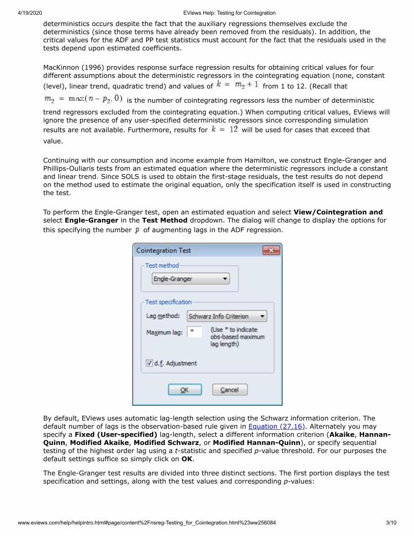
To perform the Engle-Granger test, open an estimated equation and select View/Cointegration andselect Engle-Granger in the Test Method dropdown. The dialog will change to display the options forthis specifying the number of augmenting lags in the ADF regression.

By default, EViews uses automatic lag-length selection using the Schwarz information criterion. Thedefault number of lags is the observation-based rule given in Equation (27.16). Alternately you mayspecify a Fixed (User-specified) lag-length, select a different information criterion (Akaike, Hannan-Quinn, Modified Akaike, Modified Schwarz, or Modified Hannan-Quinn), or specify sequentialtesting of the highest order lag using a t-statistic and specified p-value threshold. For our purposes thedefault settings suffice so simply click on OK.

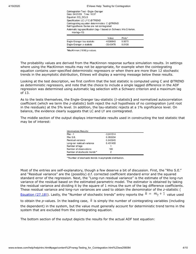
The Engle-Granger test results are divided into three distinct sections. The first portion displays the testspecification and settings, along with the test values and corresponding p-values:

http://www.eviews.com/help/content/nsreg-Estimating_a_Cointegrating_Regression.html#ww257122



The probability values are derived from the MacKinnon response surface simulation results. In settingswhere using the MacKinnon results may not be appropriate, for example when the cointegratingequation contains user-specified deterministic regressors or when there are more than 12 stochastictrends in the asymptotic distribution, EViews will display a warning message below these results.

Looking at the test description, we first confirm that the test statistic is computed using C and @TRENDas deterministic regressors, and note that the choice to include a single lagged difference in the ADFregression was determined using automatic lag selection with a Schwarz criterion and a maximum lagof 13.

As to the tests themselves, the Engle-Granger tau-statistic (t-statistic) and normalized autocorrelationcoefficient (which we term the z-statistic) both reject the null hypothesis of no cointegration (unit rootin the residuals) at the 5% level. In addition, the tau-statistic rejects at a 1% significance level. Onbalance, the evidence clearly suggests that LC and LY are cointegrated.

The middle section of the output displays intermediate results used in constructing the test statistic thatmay be of interest:

Most of the entries are self-explanatory, though a few deserve a bit of discussion. First, the “Rho S.E.”and “Residual variance” are the (possibly) d.f. corrected coefficient standard error and the squaredstandard error of the regression. Next, the “Long-run residual variance” is the estimate of the long-runvariance of the residual based on the estimated parametric model. The estimator is obtained by takingthe residual variance and dividing it by the square of 1 minus the sum of the lag difference coefficients.These residual variance and long-run variances are used to obtain the denominator of the z-statistic (Equation (27.18)). Lastly, the “Number of stochastic trends” entry reports the value used

to obtain the p-values. In the leading case, is simply the number of cointegrating variables (includingthe dependent) in the system, but the value must generally account for deterministic trend terms in thesystem that are excluded from the cointegrating equation.

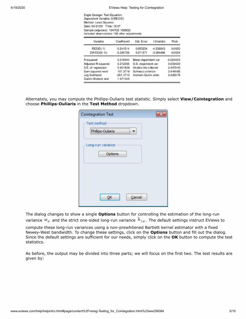
The bottom section of the output depicts the results for the actual ADF test equation:



Alternately, you may compute the Phillips-Ouliaris test statistic. Simply select View/Cointegration andchoose Phillips-Ouliaris in the Test Method dropdown.

The dialog changes to show a single Options button for controlling the estimation of the long-runvariance and the strict one-sided long-run variance . The default settings instruct EViews to

compute these long-run variances using a non-prewhitened Bartlett kernel estimator with a fixedNewey-West bandwidth. To change these settings, click on the Options button and fill out the dialog.Since the default settings are sufficient for our needs, simply click on the OK button to compute the teststatistics.

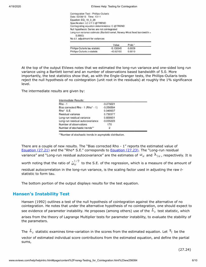
As before, the output may be divided into three parts; we will focus on the first two. The test results aregiven by:



At the top of the output EViews notes that we estimated the long-run variance and one-sided long runvariance using a Bartlett kernel and an number of observations based bandwidth of 5.0. Moreimportantly, the test statistics show that, as with the Engle-Granger tests, the Phillips-Ouliaris testsreject the null hypothesis of no cointegration (unit root in the residuals) at roughly the 1% significancelevel.

The intermediate results are given by:

There are a couple of new results. The “Bias corrected Rho - 1” reports the estimated value ofEquation (27.21) and the “Rho* S.E.” corresponds to Equation (27.23). The “Long-run residualvariance” and “Long-run residual autocovariance” are the estimates of and , respectively. It is

worth noting that the ratio of to the S.E. of the regression, which is a measure of the amount of

residual autocorrelation in the long-run variance, is the scaling factor used in adjusting the raw t-statistic to form tau.

The bottom portion of the output displays results for the test equation.

Hansen’s Instability Test

Hansen (1992) outlines a test of the null hypothesis of cointegration against the alternative of nocointegration. He notes that under the alternative hypothesis of no cointegration, one should expect tosee evidence of parameter instability. He proposes (among others) use of the test statistic, which

arises from the theory of Lagrange Multiplier tests for parameter instability, to evaluate the stability ofthe parameters.

The statistic examines time-variation in the scores from the estimated equation. Let be the

vector of estimated individual score contributions from the estimated equation, and define the partialsums,

(27.24)



where by construction. For FMOLS, we have

(27.25)

where is the residual for the transformed regression. Then Hansen chooses a

constant measure of the parameter instability and forms the statistic

(27.26)

For FMOLS, the natural estimator for is

(27.27)

The and may be defined analogously to least squares for CCR using the transformed data. For

DOLS is defined for the subset of original regressors , and may be computed using the

method employed in computing the original coefficient standard errors.

The distribution of is nonstandard and depends on , the number of

cointegrating regressors less the number of deterministic trend regressors excluded from thecointegrating equation, and the number of trending regressors in the system. Hansen (1992) hastabulated simulation results and provided polynomial functions allowing for computation of p-values forvarious values of and . When computing p-values, EViews ignores the presence of user-specified

deterministic regressors in your equation.

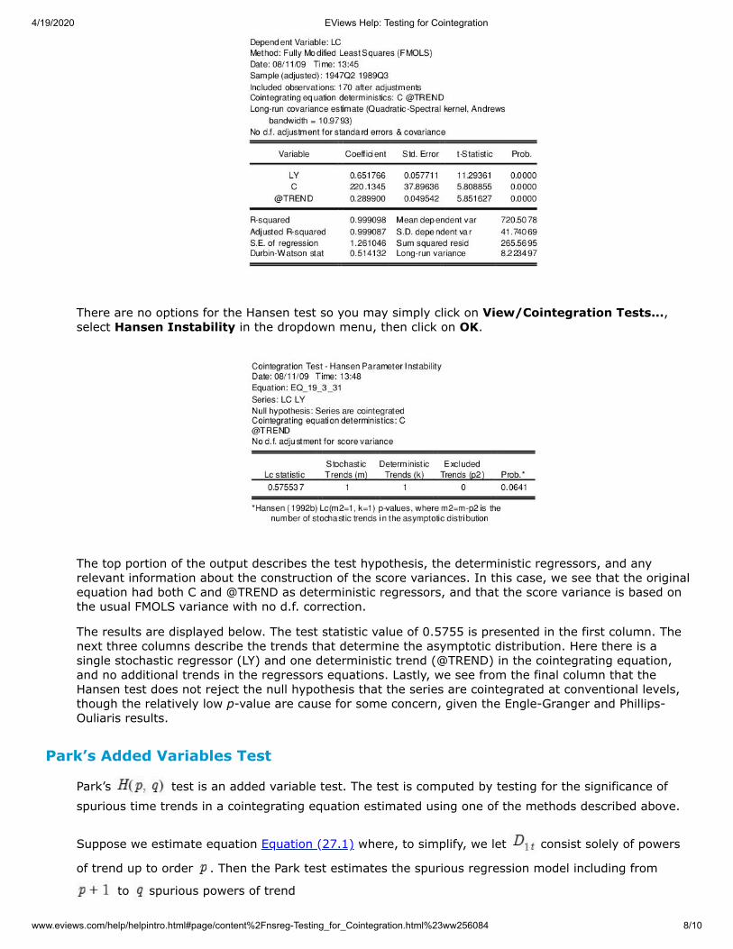
In contrast to the residual based cointegration tests, Hansen’s test does rely on estimates from theoriginal equation. We continue our illustration by considering an equation estimated on the consumptiondata using a constant and trend, FMOLS with a Quadratic Spectral kernel, Andrews automatic bandwidthselection, and no d.f. correction for the long-run variance and coefficient covariance estimates. Theequation estimates are given by:



There are no options for the Hansen test so you may simply click on View/Cointegration Tests...,select Hansen Instability in the dropdown menu, then click on OK.

The top portion of the output describes the test hypothesis, the deterministic regressors, and anyrelevant information about the construction of the score variances. In this case, we see that the originalequation had both C and @TREND as deterministic regressors, and that the score variance is based onthe usual FMOLS variance with no d.f. correction.

The results are displayed below. The test statistic value of 0.5755 is presented in the first column. Thenext three columns describe the trends that determine the asymptotic distribution. Here there is asingle stochastic regressor (LY) and one deterministic trend (@TREND) in the cointegrating equation,and no additional trends in the regressors equations. Lastly, we see from the final column that theHansen test does not reject the null hypothesis that the series are cointegrated at conventional levels,though the relatively low p-value are cause for some concern, given the Engle-Granger and Phillips-Ouliaris results.

Park’s Added Variables Test

Park’s test is an added variable test. The test is computed by testing for the significance ofspurious time trends in a cointegrating equation estimated using one of the methods described above.

Suppose we estimate equation Equation (27.1) where, to simplify, we let consist solely of powers

of trend up to order . Then the Park test estimates the spurious regression model including from

to spurious powers of trend

http://www.eviews.com/help/content/nsreg-Background.html#ww256618



(27.28)

and tests for the joint significance of the coefficients . Under the null hypothesis of

cointegration, the spurious trend coefficients should be insignificant since the residual is stationary,while under the alternative, the spurious trend terms will mimic the remaining stochastic trend in theresidual. Note that unless you wish to treat the constant as one of your spurious regressors, it shouldbe included in the original equation specification.

Since the additional variables are simply deterministic regressors, we may apply a joint Wald test ofsignificance to . Under the maintained hypothesis that the original specification of the

cointegrating equation is correct, the resulting test statistic is asymptotically .

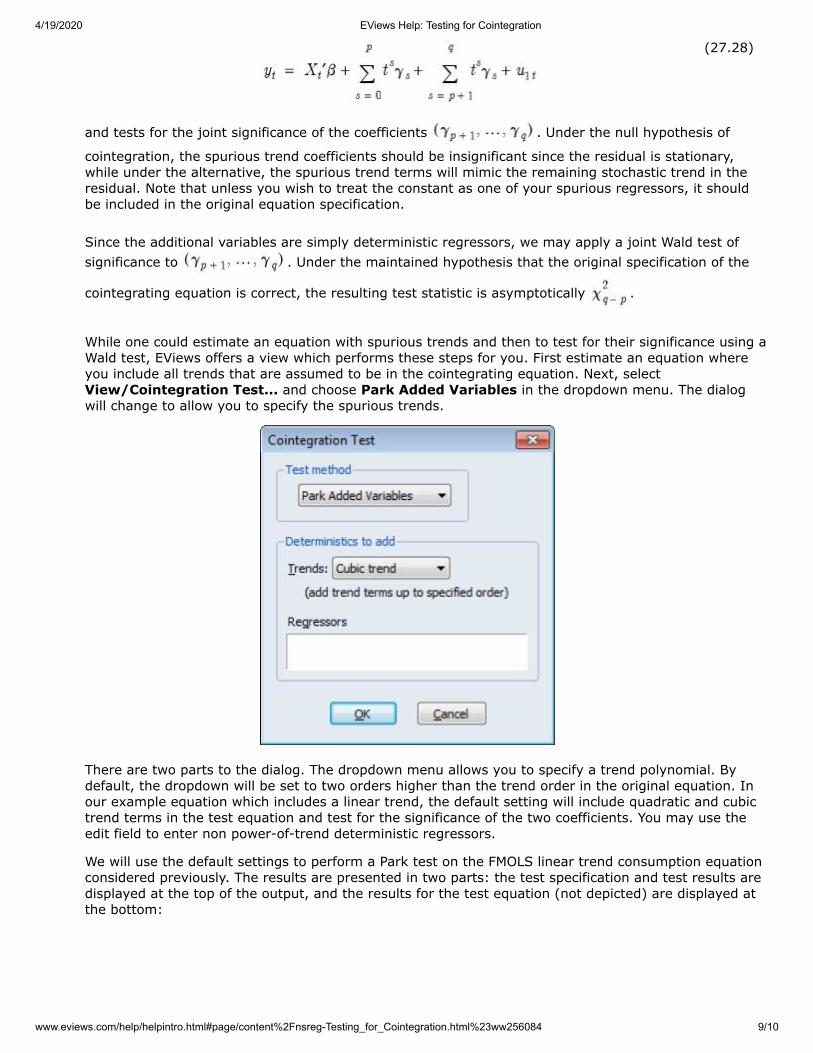
While one could estimate an equation with spurious trends and then to test for their significance using aWald test, EViews offers a view which performs these steps for you. First estimate an equation whereyou include all trends that are assumed to be in the cointegrating equation. Next, selectView/Cointegration Test... and choose Park Added Variables in the dropdown menu. The dialogwill change to allow you to specify the spurious trends.

There are two parts to the dialog. The dropdown menu allows you to specify a trend polynomial. Bydefault, the dropdown will be set to two orders higher than the trend order in the original equation. Inour example equation which includes a linear trend, the default setting will include quadratic and cubictrend terms in the test equation and test for the significance of the two coefficients. You may use theedit field to enter non power-of-trend deterministic regressors.

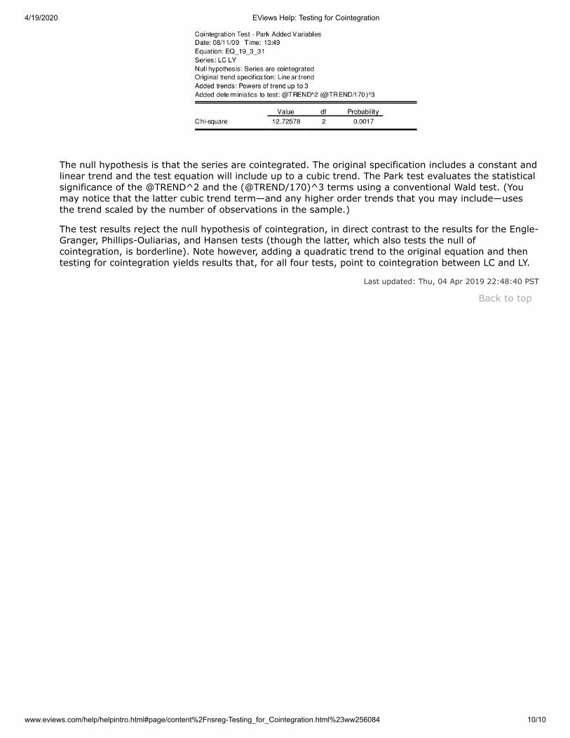
We will use the default settings to perform a Park test on the FMOLS linear trend consumption equationconsidered previously. The results are presented in two parts: the test specification and test results aredisplayed at the top of the output, and the results for the test equation (not depicted) are displayed atthe bottom:



Back to top

The null hypothesis is that the series are cointegrated. The original specification includes a constant andlinear trend and the test equation will include up to a cubic trend. The Park test evaluates the statisticalsignificance of the @TREND^2 and the (@TREND/170)^3 terms using a conventional Wald test. (Youmay notice that the latter cubic trend term—and any higher order trends that you may include—usesthe trend scaled by the number of observations in the sample.)

The test results reject the null hypothesis of cointegration, in direct contrast to the results for the Engle-Granger, Phillips-Ouliarias, and Hansen tests (though the latter, which also tests the null ofcointegration, is borderline). Note however, adding a quadratic trend to the original equation and thentesting for cointegration yields results that, for all four tests, point to cointegration between LC and LY.

Last updated: Thu, 04 Apr 2019 22:48:40 PST

Testing For Cointegration - SU LMS

Documents