Testing cointegration in infinite order vector autoregressive processes

ELSEVIER Journal of Econometrics 81 ( |997) 93-126

J O U R N A L O F Econometa'ics

Testing cointegration in infinite order vector autoregressive processes

Pentti Saikkonen .,a, Ritva Luukkonen b

aDepartnwnt o f Statistics. SF-O0014 Unit'ersity o f HelsinkL P.O. Box 54. Finland bitts'titute of Occupational Health. Topeliuksenkatu 41a A. 00250. HelsinkL Finland

Abstract

This paper studies test procedures which can be used to determine the cointegrating rank in infinite order vector autoregressive processes. The considered tests are analogs or close versions o f previous l ikelihood ratio tests obtained for finite-order Gaussian vector autoregressive processes, it is shown that the use o f the l ikelihood ratio tests is justified even when the data are generated by an infinite order non-Gaussian vector autoregressive process. New tests are also developed for cases where intercept terms are included in the cointegrating relations. These tests are based on a new approach o f estimating the intercept terms. They have the property that, under the null hypothesis, the same asymptotic distribution theory applies as in the case where the values o f the intercept terms are a priori known and not estimated. A limited simulation study indicates that the new tests can be considerably ntore powerful than their previous counterparts. © 1997 Elsevier Science S.A.

Keyi.,ords. Cointegration; Infinite order vector autoregression; Likelihood ratio test J E L ¢!assiJication: C32

1. Introduction

T h e l i t e ra tu re o n s ta t i s t ica l a n a l y s i s o f c o i n t e g r a t e d s y s t e m s has g r o w n e n o r - m o u s l y s ince the s e m i n a l pape r o f E n g l e a n d G r a n g e r ( 1 9 8 7 ) . In p rac t i ce , t he

d e t e r m i n a t i o n o f the n u m b e r o f c o i n t e g r a t i n g vec to r s , t ha t is, the c o i n t e g r a t i n g r a n k is o f t en an i m p o r t a n t par t o f th i s a n a l y s i s and , t he r e f o r e , a n u m b e r o f tes t p r o c e d u r e s have b e e n d e v e l o p e d for th is pu rpose . A m o n g the b e s t - k n o w n tes ts a re the r e s i d u a l - b a s e d tes ts i n i t i a t ed by E n g l e a n d G r a n g e r ( 1 9 8 7 ) and fu r the r

* Corresponding author. The authors wish to thank Peter Boswijk, In Choi, Atsushi Nishio, Pierre Perron and two

anonymous referees for useful comments on a previous version of this paper.

0304-4076/97/$17.00 © 1997 Elsevier Science S.A. All rights reserved Pi i S 0 3 0 4 - 4 0 7 6 ( 9 7 ) 0 0 0 3 6 - 5

94 P. Saikkonen, R. LuukkonenlJournal o f Ecom,melric.~" 81 (1997) 93-126

developed by Phillips and Ouliaris (1990), the principal components tests o f Stock and Watson (1988), and the likelihood ratio tests obtained by Johansen (1988, 1991 ) in the context o f finite-order Gaussian vector autoregressive (VAR) processes. The likelihood ratio tests, which are based on more specific assumptions about the data generating process than some of their alternatives, have become very popular in applications. In a recent paper Saikkonen (1992) showed that closely related versions o f (some of ) the likelihood ratio tests can also be derived under conditions much weaker than those originally used by Johansen (1988, 1991 ). Specifically, Saikkonen (1992) only assumed an infinite-order VAR process and approximated it by a finite-order autoregression, whose order was required to tend to infinity with the sample size at a suitable rate. It is shown in this paper that the original versions o f the likelihood ratio tests can similarly be extended to infinite order VAR processes. Another, and actually more important, contribution of the paper is that new and more powerful tests than the previous ones are developed for models with intercept terms included in the eointegrating relations. Finally, using extensions o f recent results o f Ng and Perron (1995), it is shown that all these results can be obtained by weakening previously used assumptions o f the relation between the sample size and selected order of the V A R process.

The new tests o f the paper are based on a new approach o f estimating the intercept terms o f the c,~integrating relations. The idea is similar to that already used by Elliot et al. (1996) and Pantula et al. (1994) for univariate autoregressive unit-root tests. It requires that the intercept terms are included in the model in a suitable way and estimated by using appropriate generalized least squares. The resulting test statistics have the interesting property that under the null hypothesis their limiting distributions are the same as in the case where the model contains no intercept terms or when the values of the intercept terms are a priori known. Since the limiting distributions o f the previous test statistics are affected by the estimation of the intercept terms it is intuitively expected that the new tests have good power properties compared with their previous counterparts. The simulation results of the paper confirm this intuition.

The paper is organized as follows. S~¢tion 2 contains preliminary considera- tions about the model and testing problem. Section 3 presents the considered test procedures and the asymptotic distributions of the test statistics under the null hypothesis. Section 4 studies finite sample properties o f the tests by Monte Carlo simulation. Section 5 concludes. Proofs o f the theorems are given in a mathematical appendix.

2. Prel iminaries

Following Saikkonen (1992), we consider an n-dimensional time series y t ,

t -- 1 . . . . , T, pai~itioned as

P. Saikkonen. R. LuukkonenlJournal o f Econometrics 81 (1997) 93-126 95

Y ' t=[Y~ t Y2t], nl + n z = n , (1)

n l /12

and generated by the cointegrated system

Ylt - - A y 2 t + ult, (2a)

zl y2t = u2t, (2b)

where A is the usual difference operator and ut = [u~t ' ' u2t] is a stationary process with zero mean and continuous spectral density matrix which is positive definite at the zero frequency. Hence Y2t is an integrated process o f order one which is not cointegrated while Ylt and Y2t are cointegrated. The initial value y0 may be any random vector with a fixed probability distribution.

Taking first differences and rearranging yields the triangular error correction representation

A yt = J O ' y t - t + vt, (3)

where J ' = [ - In , 0], O ' - - [ InL - A ] , and v t - - [v~ t v'2t]' is a nonsingular linear t ransformation o f ut defined by v l t - - u l t + A u 2 t and v2t =u2 t (cf. Philli0s, 1991; Saikkonen, 1992). The process vt (and hence ut) is assumed to have an infinite- order autorcgressive representation

o o

~_, G j v t - j -- e,t, G o = I n , (4) j=O

where et is a sequence o f continuous i.i.d. (0,2~) random vectors with Z7 positive definite and et have finite fourth moments . A further assumption is that the coefficient matr ices Gj are l - summable so that

o o

EJlIGjl[ <oo. (5) j = l

This condit ion imposes a slight restriction on the temporal dependence o f the process yr. It is, for example, satisfied by all stationary and invertible A R M A processes and it implies that the process vt and, consequently, yt can be approximated by a finite-order autoregression (see Saikkonen, 1992). Specifically, f rom (3) and (4) one can obtain the approximate model

K A y t = qJYt- i + ~ l l j A y t _ j + et, t = K + 2, K + 3 , . . . , (6 )

j = !

where o o

e , = ~ . - E Gjv,-i. j=K+ i

96 e. Saikkonen, I{ LuukkonenlJournal o f Econometrics 81 (1997) 03-126

Here K is supposed to be so large that Gi ~ O, j > K, so that et ~ e.t. Furthermore, due to cointegration, the coefficient matrix q~ has reduced rank and the structure

K ~, = ~ o ' = - ~ G j J O ' , (7)

j=O

where the second equal i ty defines the n x nl matrix 4~ which is o f full col- umn rank (at least for K large enough). Details o f the derivation o f (6) can be found in Saikkonen (1992) and Saikkonen and Liitkepohl (1996) and are not repeated here. i We note, however, that the coefficient matrices I l j ( j = 1 . . . . . K )

are functions o f O and Gy ( j = 1 ,2 , . . . ) , and, l ikewise ~ , they also depel,d on K. Furthermore, the sequence H / ( j = 1 . . . . . K ) is absolutely summable as K ~ ¢x~.

In practice, it is usual that the cointegrat ing rank, that is, the integer n~ is a priori not known. Therefore, it is o f interest to consider testing the null hypothesis

H(nl ): Cointegrat ing rank equal to hi .

Since the number o f free elements in the parameter matr ix ~ increases with nl the natural alternative hypothesis in this setting is

l~(nl ): Cointegrat ing rank larger than n,.

Note that the tbrmulat ion implies that 0 ~< n~ < n. In addit ion t o a known cointegrat ing rank, the model specification in (2) also

assumes a particular normalizat ion o f the cointegrat ing vectors. This is seen in the definition o f the coefl~riel)) matr ix O whose first n l rows form an identi ty matrix. An equivalent way o f expressing this is that, possibly after rearranging the order o f components , the vector y t can be decomposed as in ( I ) with Y2t not cointegrated. It is possible that this decomposi t ion is performed incorrectly in practice so that one might x: : .k )o test the validi ty o f the imposed normal iz ing restrictions, assuming that the cointegrat ing rank is correct ly specified. Saikkonen (1992) develops a test for this purpose. Similar tests could also be considered in the present context but this topic is outside the scope o f this paper.

As the above discussion makes clear, the hypothesis H(n~ ) is equivalent to the existence o f the tr iangular error correction representation (3) with the rows o f the matrices J and O or the components o f the vector Yt possibly permuted. This alternative formulat ion o f the hypothesis is somet imes convenient. Since the test procedures discussed in this paper are invariant to a permutat ion o f the components o f Yt it can a lways be assumed in theoretical derivat ions that the

t The present formulation of the model is similar to that used in Saikkonen and Ltitkepohl (1996) and also in the appendix of Saikkoncn (1992). it is slightly simpler than the one given on p. 4 of Saikkonen (1992) where the definition of the matrix 4~ does not involve K and consequently the error term et is slightly more complicated than here. Condition (5) implies that the difference between these two formulations is asymptotically negligible in the sense that thc two definitions of the matrix 4~ differ by a quantity which is of order o(K - t ) (see Saikkonen, 1992, Eq. (A.17)).

P. Saikkonen, R. Luukko,~en l Journal o f Econometrics 81 (1997) 93-126 97

da ta genera t ing process satisfies ( 2 ) and (3) . Th i s is the ma in reason w h y the normal i z ing res t r ic t ions are used in this paper .

The above mode l a s s um e s that there is no intercept in the co in tegra t ing rela t ion (2a) . Since this is ra ther se ldom a real ist ic a s sumpt ion it is reasonable to cons ide r a mode l which a l lows for this feature. Suppose w e now obse rve an n -d imens iona l t ime series zt , t - - 1, . . . . T , which is genera ted b y

zt - - m q- Yt, ( 8 )

where m (n x 1 ) is an u n k n o w n p a r a m e t e r vec to r and Yt is as in ( 2 ) or, equ iva- lent ly, (3) . Mul t ip ly ing ( 8 ) f rom the left b y 19' and [0 In2]A yie lds

z l , = It + Az2, + u l , , ( 9 a )

Az2, = u2,, ( 9 b )

w h e r e / ~ = O ' m whi le z l t and z2t are obv ious subvec tors o f zt . This is the exten- s ion o f ( 2 ) cons ide red b y Sa ikkonen (1992) , w h o poin ted out that, ana logous ly to (6) , one can obta in f rom (9 ) the app rox ima te mode l

K Az~ = v + qJzt-~ + ~ l l y A z t _ j + el, t = K + 2 , K + 3 . . . . ( 6 ' )

j----!

where t/, satisfies (7) , v = - - O / ~ , and et is as d e £ n e d be low (6) . 2 Since v = - - O O ' m = - tPm it fo l lows f rom ( 6 ' ) that

K Azt = tP(z t_ t -- m ) + ~ H j A z t - j + et, t = K + 2 , K + 3 , . . . . ( 6 " )

j=l

The null hypo thes i s H(n l ) can also be cons ide red wi th in mode l s ( 6 ' ) and ( 6 " ) . A diff iculty wi th the lat ter m ode l is that it is non l inea r wi th respect to the level pa rame te r m and, unl ike ( 6 ' ) , canno t be es t imated b y o rd inary least squares . It turns out, however , that .~t is wor thwhi l e to pay for this compl ica t ion . T h e s imula t ion resul ts o f Sect ion 4 indicate that test p rocedures based on mode l ( 6 " ) can be subs tant ia l ly more powerfu l than those based on (6 ' ) .

3. Test procedures

3.1. M o d e l s w i t h o u t a n i;2tercept

The es t imat ion and tes t ing p rocedures in Sa ikkonen ( 1 9 9 2 ) are based on the unres t r ic ted leas t -squares es t imat ion o f a m i n o r modi f ica t ion o f (6) . T h e

2 Unlike in Saikkonen (1992) the same error term et appears both in (6) and (6t). As Eq. (9") of Saikkonen (!~92) r,mkes clear, the reason is that here the matrix 4b is allowed to depend on K. (Note also the printing error in the definition of the error term e~' below Eq. (9') of the previous paper. The correct definition should contain J/~ in place of/~.)

9 8 P. Saikkonen, R. LuukkonenlJournal o f Econometrics 81 (1997) 93-126

modificat ion takes explici t ly into account the fact that the first n~ columns o f the coefficient matr ix I lK are zero vectors. The purpose o f the modification was only to s impl i fy mathemat ical derivations and, since it has no effect on asymptot ic results, it will not be used in this paper. Thus, we define xt = [Ay ' t_ 1 . . . A Y ' - K ] ' and H----[Hi . . . ILK], and write the est imated version o f (6) as

A y t = ~ Y t - t + f l x t + ~:t, t = K + 2 , . . . , T, ( lO)

where ~' and / 7 - - [ / 7 1 . . . /TK] are the ordinary least-squares est imators o f the coefficient matrices tp and H, respectively. The error covariance matr ix ,~ is es t imated by

T

£ N - I - - ' ~t ~ t • t = K + 2

where N = T -- K -- 1. Let 2t ~< - " - ~< 2n be the solutions o f the general ized eigenvalue problem

- z £ t = 0 , (11)

where

r r ~- -~+) / r2xtx \ - i r t _ t X ¢ C ' ~ " ~ Y [ - ]Y! - - | E J | - - l . . . . X', E /y/__ | • t~.K+2 t = K + 2 t t - - - -K+2

In order to test the hypothesis H(ni ) we now introduce the test st-..sii.~

/12 w=Z G.

j=l

It is clear that this test statistic is invariant to the " ~qmalization o f the cointegrat ing vectors and its large values are critical.

Test statistic W is a slight modificat ion G • test statistic R discussed in Saikkonen (1992) . This latter test statistic ¢~: :.e defined in the same way as test statistic W except that th~ i . . . . . :. C it. ( i i I is replaced by

T

M ' - ~, y,_,y~_,. (12) t = K + 2

Thus, in the present version o f the test statistic the matr ix M is corrected for the short-run dynamics o f the process. This correction has some appeal because it takes the intertemporal dependence o f the data into account. It also makes the test very close to the l ikelihood ratio test developed by Johansen (1988) for finite-order Gaussian V A R processes. The l ikelihood ratio test statistic is obtained by techniques similar to those employed in reduced rank regression. In fact, it

P. Saikkonen. 1~ Luukkonenl Journal of Econometrics 81 (1997) 93-126 99

is not difficult to check that in our context an analog of the likelihood ratio test statistic is

n2

LR ---- N~--~ log( l + f~jlN) j = l

(cf. Anderson, 1951, Eq. (3.2)). This expression of the likelihood ratio test statistic differs from the one given by Johansen (1988). However, the two expressions are identical since in our notation Johansen (1988) uses the transformed eigenvalues ~ j / ( N + ~j ) ( j - - I . . . . . n2).

To be able to obtain the limiting distributions o f the above test statistics some assumptions are needed. Since we only use a finite-order autoregression as an approximation we have to assume that its order tends to infinity with the sample size T at a suitable rate. Therefore, we shall make the following assumption which has previously been used by several authors (see e.g. Berk, 1974; Lewis and Reinsel, 1985; Said and Dickey, 1984; Saikkonen, 1991, 1992; and Saikkonen and Lfitkepohl, 1996).

A s s u m p t i o n 1. K is chosen as a function 6 f T such that f - - - , oo and K 3 / T - - , 0 as T ---, c~.

Thus, we impose an upper bound for the rate at which the autoregressive order K is allowed to tend to infinity with the sample size. In most previous studies in the area, like those referred to above, it has also been assumed that the autoregressive order satisfies a lower bound condition, na.~nely,

o o

T '/2 IIGjlI 0 as T-- ,oo. (13) j---:K+l

However, recently Ng and Perron (1995) pointed out that this condition is actually not needed to obtain the limiting distribution o f the univariate unit root test o f Said and Dickey (1984). Since our test procedures can be thought of as extensions o f this univariate unit root test it is no wonder that condition (13) can also be removed in this context.

Being able to remove the lower bound condition (13) has also some practical implications concerning the choice o f the autoregressive order K. For instance, suppose one uses some common model selection criterion, like AIC or BIC, to choose an appropriate value of K. In the important special case where the data generation process has an A R I M A structure the selected order will then tend to infinity at the rate Op(Iog T), as shown by Ng and Perron (1995) and Saikkonen (1995). This means that the selected order is generally not consistent with the lower bound condition (13) although it is consistent with Assumption I. It is also shown in Saikkonen (1995) that, under conditions essentially the same as we have assumed here, the application o f all conventional model selection criteria

I00 P. Saikkonen. R. L u u k k o n e n l J o u r n a l o f Econometr ics 81 (1997) 93-126

will yield an order which tends to infinity in probability. This is again consistent with Assumpt ion 1. A detailed discussion o f the use and properties o f data-based order selection methods is outside the scope o f this study, however.

Unless otherwise stated Assumpt ion 1 is supposed to hold throughout the paper. It will be convenient to denote

~ ( n 2 ) = t r ( ~ W ( r ) d W ( r ) ' ) t (lfo W ( r ) W ( r ) ' d r ~

where W(r) is an n2-dimensional standard Brownian motion. N o w we can state the fol lowing theorem where the hypothesis H(n~ ) is assumed and the symbol ' - - - - > ' is used to signify weak convergence o f the associated probabil i ty mea- sures.

Theorem 3.1. Suppose that Yt (t = 1 . . . . . T) is generated by (3) and (4 ) with the rows o f J and 6) possibly permuted. Suppose further that Assumption 1 holds. Then, W ~.. ~(n2) and LR .~ ~(n2), as T ~ oo.

The p roof o f Theorem 3. i is given in the appendix where it is shown that test statistic W and its previous version R and related by W = R + op( 1 ). When the order o f the considered V A R process is fixed and finite this result is straightforward to obtain but some complicat ions occur when the order is a l lowed to tend to infinity. From the definitions it is also easy to deduce the LR = W+op( 1 ). Thus, under the hypothesis H(ni ), the three test statistics are asymptot ica l ly equivalent and have the same lirniting distribution as the l ikelihood ratio test statistic in the case o f a finite-order Gaussian V A R process.

3.2. Models with an intercept

The test procedure o f Sa ikkonen (1992), which al lows for an intercept, is based on an est imated version (6 ' ) , that is, on

A Z t = V + g v Z t . _ l + J ~ v X t " ~ v t , t = K + 2 . . . . . T, (14)

where "~, W~. and / lv := [/l~.i . . . /I,.K] are ordinary least squares est imators o f the parameters v, tp and H , respectively. Notice that, due to the relation Azt = Ayt, t > 1, the vector xt also appears here and is defined as x t - [Az~_ l . . . AZt_K]' '. In this case the error covariance matrix Z" is est imated by

T :.~ N -l W. " " = ~ v t ~ , t .

t =K +2

P. Saikkonen. R. LuukkonenlJournal of Econometrics 81 (1997) 93-126 101

An analog o f test statistic W can now be obtained in an obvious way. Let ~.vl ~< "'" ~< ~.v,, be the solutions o f the generalized eigenvalue problem

v,~cv,~ - : . ~ 1 = o

where

T ~ = ~ ~ , - , ~ , - , -

t = K + 2

T / T --\--I T Y~ - - ' ~ - - ' / - - t=K+2 t = K + 2 / t = K + 2

(15 )

with ~'t-! and ~t demeaned versions o f the series zt- i and xt, respectively. In other words, ~'t- i = z t - m -- £'- i and £t = xt - £ where ~_ ~ and .~ are the sample means o f z t - ~ and xt (t = K + 2 , . . . , T), respectively. In place o f test statistic W we now have

n2 ,,.

j = l

The analogous previous test statist';e discussed in Saikkonen (1992) and denoted by Re here is defined in the same way as test statistic W~ except that the matrix C" in (15) is replaced by

T

t = K + 2

An obvious analog o f the likelihood ratio test statistic is now

tt2 LRv = N ~ log(I + ~v,/N).

j = l

The fol lowing t~¢orem shows that, under the hypothesis H(ni ), test statistics W~ and LRv have the same limiting distribution as test statistic Rv and tim corresponding likelihood ratio test statistic obtained by Johansen (1991) for finite order Gaussian V A R processes. The limiting distribution can be represented by the random variable

~ (n2) - - t r ( 0 ~ l~'(r)dW(r) ') ' ( ~ 14,'(r)W(r)' d r ~ I

x ( ~ , Y ( r ) d W ( r ) ' )

where l ~ ' ( r ) = W ( r ) - f~ W(s)ds (0 <~r<~ l ) is a demeaned Brownian motion.

Theorem 3.2. Suppose that zt (t--- 1 . . . . . T) is oenerated by (8) and chat the assumptions stated in Theorem 3.1 hold. Then, W~ ~. ~(n2) and LRv --~- ~(n2), as T---> cx~.

! 0 2 P. Saikkonen. IZ LuukkonenlJournal o f Econometrics 81 (1997) 93-126

Next, we shall consider tests based on model (6" ) . The idea is to replace the level parameter m by an appropriate es t imator and proceed in the same way as in Section 3.1 or, equivalently, when the value o f m is known. A major problem with this approach is the est imation o f m. Since v = - ~ m , a natural est imator is - - ~ ' f ~ ¢ but this is not a good choice since, due to the asymptot ic singulari ty o f the matr ix ~, , it d iverges as the sample size tends to infinity. Specifically, using results in Saikkonen (1992, 1995) it is not difficult to show that in some directions o f the parameter space the rate o f divergence is as fast as Op(T) . To find a better estimator, first define

t - - ! d, ==, - & : , - j ,

} = i t -- 1 . . . . . K + 1,

and

K + I

j = l t - - K + 2 . . . . . T,

where /}v, = In + ~v + lZlvl, B~j = ffl , j - f f l , . j _ t , j = 2 . . . . . K , and/}v.g+i = - - / l , g . From these definitions and (14) it can be seen that /}~/ ( j = 1, . . . . K + I ) are least-squares estimators obtained by fitting an autoregression o f order K + ! to the levels series so that z t = ~ + B ~ t z t - l + " "" + B~.K + l z t - g - ! + ~:~t ( t = K + 2 . . . . . T ) and In - - / ~ , . . . . . /~v.K+l = -- ~U, (Cf. Saikkonen and Liitkepohl, ! 996 below (2.8)) . Next define C ' l - - I , ,

t - - I C t = l n - - Y~ .Bv j , t = 2 . . . . . K + 1,

j = !

and Ct = -tp,. for t = K + 2 . . . . , T. Note that we can also write C't = - ~ . - / J r , t - ! for t = 2 . . . . . K + 1. With these definitions we now introduce the est imator

1

To see the motivat ion o f this estimator, consider ( 6 " ) augmented for t = 1 . . . . , K + 1 with the miss ing pre-sample observat ions assumed to be z t = m, t = - - K , . . . , 0. Then, i f Bt . . . . . B x + t denote the autoregressive coefficient matrices o f the levels formulat ion o f the model, we have

t - - ! z , = m + ~ B j ( z j -- m ) + et ,

j---I

K + i z t = m + Y]~ B j ( z j -- m ) + et ,

j=i

t - - I , . . . , K + I

t - - K + 2 , K + 3 . . . . .

(16)

P. Saikkonen, 1~ LuukkonenlJournal o f Econometrics 81 (1997) 93-12o 103

O f course, the relation between the coefficient matrices By (j---- I, . .. , K 4 - 1 ) , and / / j ( j - - 1 . . . . . K ) is exactly the same as the relation between the cor-

responding est imators described above. Suppose that zt in (16) is a Gaussian V A R process o f a fixed and finite order K 4- 1. Then, et : Et ~-, n.i.d.(0, E ) and, i f

/~j ( j -- 1 . . . . . K ÷ 1 ) and ~ were m a x i m u m likelihood est imators based on (16) , the est imator ~fi would clearly he the m a x i m u m likelihood est imator o f the parameter m. O f course, we do not have m a x i m u m likelihood est imators but this observation shows that the est imator ~fi can be interpreted as a first step in an iterative m a x i m u m likelihood estimation algorithm. The next step would be to replace m in (16) by the est imator ~ and obtain obvious new estimators for the parameters By ( j - - 1 . . . . . K 4- 1 ) and 2:. Iterating this procedure until convergence yields m a x i m u m likelihood estimators. The est imator t~ can thus be motivated as an approximate m a x i m u m likelihood estimator. The approximation results he- cause the procedure is not iterated and because our assumptions arc more general than those assumed above. This interpretation o f the est imator n~ was suggested by a referee. Since the error term e, in (16) is approximately white noise with covariance matrix Z the est imator t~ can alternatively be interpreted as a feasible version o f an approximately optimal general ized least-squares estimator.

Asymptot ic properties o f the est imator ~ are given in the fol lowing l emma where J~ -- [0 In2].

Lemma 3.1. Suppose that zt (t = 1, . . . . T) is generated by (8) where yt satisfies (3) and (4). Suppose further that Assumption 1 holds. Then, O ' ( t ~ - m ) - - O p ( T -1/2) and J~(sfi -- m)=op(Kl /2) .

The first result o f L e m m a 3.1 shows that linear combinat ions o f ~ determined by coi1~tegrating vectors are consistent est imators o f corresponding linear com- binations o f m. The order o f consistency is the. usual one, that is, Op(T- l /2 ) . Since O'm = p and O'----[In, --A] an est imator of tt can be constructed f rom n~ and an est imator o f A. Suppose an est imator A has the usual super consistency property A = A 4 - O p ( T - ! ). Then, i f ~ ' = [In, --,4], L e m m a 3.1 implies that ~ ' ~ - - O ' t ~ - - o p ( T -~/2) and e ' t f i is an est imator o f p with the same asymptotic properties as O't~. Using the results in the p roof o f L e m m a 3. ! and those in Saikkonen (1992, 1995) it is possible to derive the l imiting distribution o f O ' ~ . This result is omitted, however, because it is not needed in this paper.

The second result o f L e m m a 3.1 implies that linear combinat ions o f n~ which are not determined by cointegrating vectors are not consistent est imators o f corresponding linear combinat ions o f m. In fact, in the direction o f J± the est imator

n~ can diverge but only at the slow rate Op(K-m/2). This s low rate o f divergence suffices for our p u r p o ~ s although better results can be obtained with stronger assumptions. For instance, i f the lower bound condition (13) is assumed one can readily show that J~0fi -- m ) - - O p ( l ) ( see the proo f o f L e m m a 3.1). As a comparison, recall that the est imator _ ~ - m ~ always diverges at the rate Op(T) .

104 P. Saikkonen, t~ LuukkonenlJournal o f Econometrics 81 (1997) 93-126

Analogous results have previously appeared in some univariate unit root tests in which the intercept is not identified and therefore its estimator is not consistent (see Schmidt and Phillips, 1992; Elliot et al., 1996). In the present context the inconsistency of J [ ~ can similarly be thought o f as a consequence of an identification problem.

Now, we can introduce the final test statistics o f this section. Replace the unknown level parameter m in (6 " ) by the estimator r~ and consider the least- squares regression

A z t - - - @ m ( Z t - 1 - - 1 ~ ) - ~ - l T m x t - ~ m t , t = K + 2 , . . . , T , (17)

where ~m and /lm----[/Tml --. /lmK] are ordinary least-squares estimators of the parameters ~P and / / , respectively. Although -~v or any other consistent estimator o f the error covariance matrix could be employed we shall use the estimator based on (17), i.e.,

T

t : - K + 2

Let ~ml ~< " '" ~< ~,-n be the solutions o f the generalized eigenvalue problem

[@me@" -- AZml--0, (18)

where ¢~ is defined by replacing Y t - ! in the definition of C by Yt-i : - z t - i - - t f i

and defining x t again as x t = [Az~_ ! . . . Az~_K]'. With these definitions we can now define test statistic

//2

W m - - Y~ ~mj j=!

which is an obvious analog of test statistic W defined in the previous section. An analog of the previous likelihood ratio type test statistic can correspondingly be defined as

n2

LRm = N l o g ( 1 + j=l

It is worth noting, however, that even if the data are generated by a Gaussian V A R process o f a fixed and finite order K + 1 test statistic LRm is not a proper likelihood ratio test statistic. In this respect it differs from test statistics LR and LR~. The obvious reason is that the estimators in (18) are not maximum likelihood estimators although they can be interpreted as approximate maximum likelihood estimators and therefore test statistic LRm can be motivated as an approximate likelihood ratio test statistic.

The limiting distributions of test statistics W,, and LR,n are given in the following theorem.

P. Saikkonen. 1~ Luukkonen l Journal o f Econometr ics 81 (1997) 93 -126 105

T h e o r e m 3.3. U n d e r the c o n d i t i o n s o f T h e o r e m 3.2, W,n ~(n2) a s T - - , o o .

;. ~(n2) a n d LRm

Thus, under the null hy)othes is test statistics W,,, and LR., have the same limiting distribution as their analogs W and LR obtained when the value o f the level parameter m is known. The l imiting distribution is therefore different f rom that o f test statistics Wv and LRv and the associated asymptot ic critical values are considerably smaller than f~ose o f test statistics Wv and LRv (see e.g. Reinsel and Ahn, 1992). This suggests that tests based on test statistics W., and LR., should be m.qre powerful than tests based on test statistics W~ and LR,,. The simulat ion results o f the next section show that in general this is indeed the case.

We close this section with a discussion o f some related test procedures. Referees have commented on the relation between test statistic LRm and the l ikelihood ratio test statistic obtained in Theorem 2.2 o f Johansen (1991) in the context o f a Gaussian finite-order V A R process (see also Johansen and .luselius, 1990). In our case this test is related to testing the joint hypothesis qJ = O O ' and v - - - O / t in (6 ' ) . It is not difficult to see that this test can be based on the general ized eigenvalue problem

I q ' * c * q '* ' - ,,t$',,I = o ,

where ~'* --[~v ~] and

T ,i T t ( c * = = ; _ , z , _ , - E \ t=K+2 t=K+2

(19)

T / - I T X t ~ t _ I

t t=K+2

with z t = [ z ~ !] ' . I f A~<- - -~< '~n are the solutions o f (19) then this approach yields the test statistic

n2 LR* = N ~ log( 1 + ~ / N ) .

j=l

It was pointed out by a referee that, using results from parti t ioned regression, one readily f n d s that solving the general ized eigenvalue problem (19) is equiva:~nt to performing a reduced rank regression on

Azt = Lt'(zt_m - ffzv) + l l x t + ~t, t = K + 2 , . . . , I", (20)

~--i where ~v =--~Pv ~ Thus, the difference between test statistic LR* and our test statistic LR,. is that different est imators are used for the parameter vector m. As we already noted, the est imator ~,, has the undesirable property that it diverges in the direction o f J ± at the fast rate Op(T) . This implies that the l imiting distribution o f test statistic LR* is different f rom that o f test statistic LR,. or from what is obtained when the value o f m is known. In the case o f a Gaussian finite

106 P. Saikkonen. P~ LuukkonenlJournal o f Econometrics 81 (1997) 93-126

order V A R process the limiting distribution o f test statistic LR* is obtained in Theorem 2.2 o f Johansen (1991) and we would expect that the same result also applies in our more general context, although no formal proof will be provided. The above derivation o f test statistic LR* is interesting, however, because it moti- vates the search for alternative estimators o f m whose properties in the direction o f J_L are better than those o f ~v. The estimator ~ used in this paper is one possibility in this respect although other estimators, like iterated versions o f n~, might also be considered. It can be seen from the appendix that the results o f Theorem 3.3 do not change if n~ is replaced by any other estimator ~* with the properties O ' ( ~ * -- m) - - Op(T -1/2) and J_L(m* -- m) - -op (Kl /2 ) . T h i s implies, for instance, that any estimator n~* satisfying t~* - - i ~ - - O p ( T - I /2) can be used in place o f t~.

Other related test procedures have been obtained in the univariate special case n = n2 = 1. First note that in this case test statistic Wm provides a new test for testing a unit root in univariate infinite-order autoregressive processes. When stationary alternatives are considered one should use the obvious square root o f Wm, however, because in that case the testing problem is one sided. The test obtained in this way is similar to the two step version o f a test developed by Pantula et al. (1994) for the first-order Gaussian autoregressive process. These authors make the same initial value assumption as in (16) and base their test on the maximum likelihood estimator o f the autoregressive parameter. They also discuss extensions to higher order autoregressive processes. Another related univariate test is the DF-GLS ~' test o f Elliot et al. (1996) which is asymptotically equivalent to the test based on the above-mentioned special case o f test statistic Win. Elliot et al. (1996) show that their test has optimal power in large samples. There are two major differences between the approach of these authors and the present one. First, when Elliot et ai. (1996) estimate the level parameter by generalized least squares they do not use an estimator o f the autoregressive parameter but employ a chosen value local to unity. This is feasible in the univariate case bat seems difficult to apply in the present context because the counterpart o f the autoregressive parameter is the matrix q& The second difference is that Elliot et al. (1996) do not take the short-run dynamics o f the process into account in the generalized least-soLuares estimation o f the level ~ e ~ r . In our case this would mean using dz t -- ~Pvzt-I and --~'v in place o f dt and Ct, t >12, respectively.

4. Simulat ion study

In this section we will report results o f a limited simulation study which ex- amines the finite sample sizes and powers o f the test procedures described in the previous section. The two models used in this simulation study are take~ from a recent paper o f Yap and Reinsel (1995). One o f them is a second order V A R

P. Saikkonen. R. Luukkonen/Journal o f Econometrics 81 (1997) 93-126 107

model and the other one a first-order A R M A model . 3 Since in practice intercept terms are almost a lways included in cointegration relations, the test procedures o f Section 3.2, which are designed for this case, are only considered.

In al! exper iments we used the sample size T = 2 0 0 and the nominal 5% significance level. The number o f replications was a lways 10000. In the generated series the normal ly distributed innovations ~t were obtained by using a r andom number generator in the N A G subroutine library on a V A X 8800 computer at the Universi ty o f Helsinki.

4.1. A s e c o n d - o r d e r J A R p r o c e s s

In our first exper iments a trivariate second order autoregressive process was considered and the series were generated by

Azt -~ tllzt_! d - F l l A Z t _ l d-e.t, t = 1 , . . . , 2 0 0 , (21)

where zo = z - ! - - 0 and Et ,-~ n.i.d.(0,2~). The parameter matr ices are defined as follows:

[ - - 0 . 0 8 0 0.224 --0.152"] [0 .47 0.20 0 .18 ] I l l = 0.177 0.046 -0.254 / , E = 0.2_'? 0.32 0.27

0.000 --0.102 0.129.1 0.18 0.27 0.30

and ~u = C d i a g ( ~ l , ~ 2 , ~ b 3 ) C -1 -- 13 with

--0.29 --0.47 - - 0 . 5 7 ] C -~ = --0.01 --0.85 1.00 .

- 0 . 7 5 1.39 --0.55

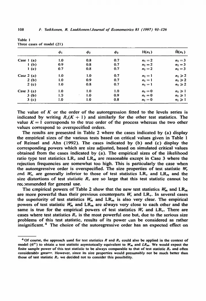
Fol lowing Yap and Reinsel (1995) , we considered three different cases described in Table 1 where, in each case, the first row (a) corresponds to the situation under the null hypothesis whereas the second and third rows (b) and (c) correspond to situations under the corresponding alternative hypothesis . Thus, the value ~bi = 1 indicates a unit root in the process and the number o f the ~i parameters less than unity indicates the number o f cointegrat ion relations. One would expect that cases where the value o f a ~b~ parameter is close to but be low unity are difficult for the tests because then the process contains a l ong -memory stationary componen t which is not easy to separate f rom nonstat ionary int~;grated components .

For each case and each replication, we computed values o f test statistics Rv, W~, LRv, Wm and LRm for testing the null hypothesis H(n l ) . Three different values o f the order parameter K were considered. They were K = 1,3 anti 5.

3 These models were taken from a discussion paper version of Yap and Reinscl (1995). Unfomt- nately, the models given in the discussion paper were slightly different from those in the published article although the reported simulation results were the same in both cases. This apparently explains the discrepancy which can be seen between some of our results and those reported by Yap and Reins¢l (1995).

108 ~. Saikkonen, R. LuukkonenlJournal o f Econometrics 81 (1997) 93-126

Tab le I Three cases o f mode l ( 2 1 )

01 02 03 H(n! ) H(nl )

Case ! ( a ) 1.0 0.8 0.7 nl = 2 nl = 3 I ( b ) 0.9 0.8 0.7 nl ~ 2 n! -~ 3 I ( c ) 0.7 0.8 0.7 n j = 2 n~ = 3

Case

Case

2 ( a ) 1.0 1.0 0.7 n! = I nl i> 2 2 (b ) 1.0 0.9 0.7 nl = I n! > / 2 2 ( c ) 1.0 0.8 0.7 nl = i nl i> 2

3 ( a ) !.0 1.0 1.0 nl = 0 nz i> 1 3 ( b ) I.D 1.0 0.9 nl = 0 nl /> 1 3 ( c ) 1.0 i .0 0.8 nl ----0 nl 1> I

The value o f K or the order o f the autoregression fitted to the levels series is indicated by writing Rv(K + 1 ) and similarly for the other test statistics. The value K = 1 corresponds to the true order o f the process whereas the two other values correspond to overspecified orders.

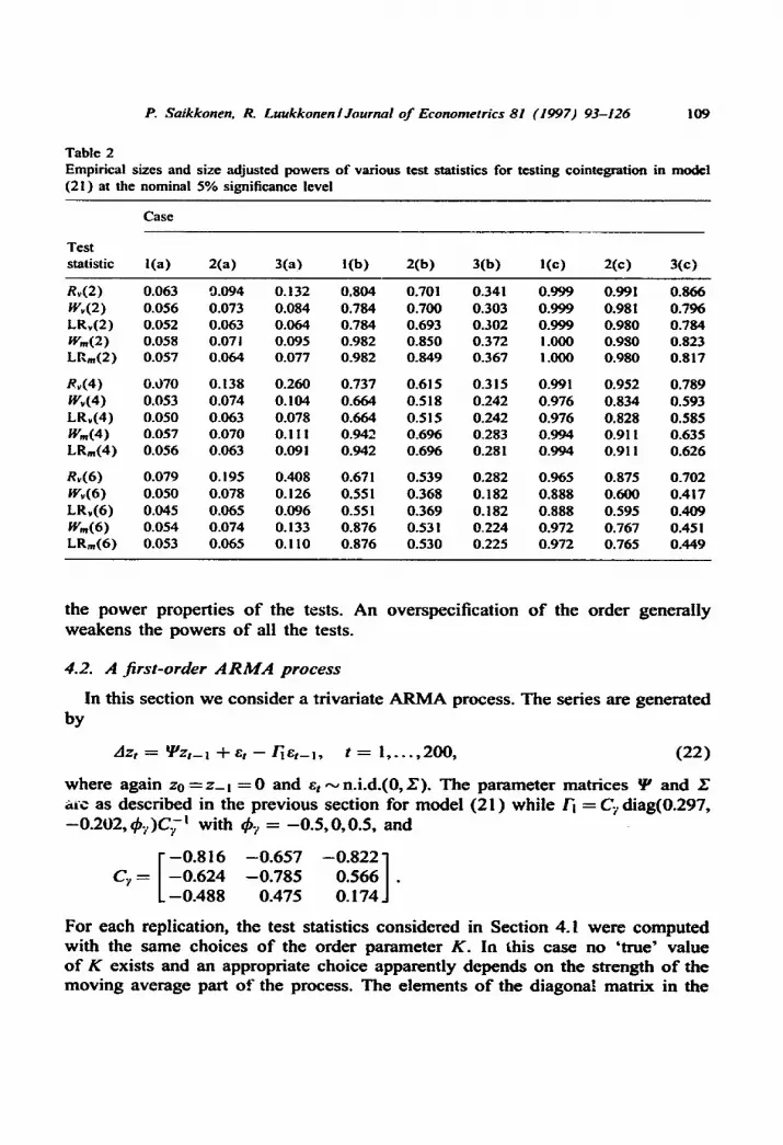
The results are presented in Table 2 where the cases indicated by (a) display the empirical sizes o f the various tests based on critical values given in Table 1 o f Reinsel and Ahn (1992). The cases indicated by (b) and (c) display the corresponding powers which are size adjusted, based on simulated critical values obtained from the cases indicated by (a). The empirical sizes o f the likelihood ratio type test statistics LR~ and LRm are reasonable except in Case 3 where the rejection frequencies are somewhat too high. This is particularly the case when the autoregressive order is overspecified. The size properties o f test statistic W~ and W.; are generally inferior to those o f test statistics LRv and LR,~ and the size distortions o f test statistic Rv are so large that this test statistic cannot be rec3mmended for general use.

The empirical powers o f Table 2 show that the new test statistics Wm and LRm are more powerful than their previous counterparts W~ and LRv. In several cases the superiority o f test statistics Wm and LRm is also very clear. The empirical powers of test statistic Wm and LRm are always very close to each other and the same is true for the empirical powers of test statistics ~K. and LRv. There are cases where test statistics Rv is the most powerful one but, due to the serious size problems of this test statistic, results o f its power can be considered as rather insignificant. 4 The choice o f the autoregressive order has an expected effect on

4 O f course , the approach used for test statistics R and Rv cou ld a lso be appl ied in the context o f m o d e l (6 H) to obta in a test statistic a symto t ica l ly equ iva len t to Wm and LRm. W e w o u l d expec t the finite sample p o w e r o f this test statistic to be a l w a y s c o m p a r a b l e to that o f tes t statistic Rv and oRen cons ide rab ly grea,~,r. H o w e v e r , s ince its size proper t ies w o u l d p r e s u m a b l y not b e much bet ter than those o f test statist ic Rv w e dec ided not to cons ider this possibi l i ty .

P. Saikkonen, R. Luukkonen/Journal o f Econometrics 81 (1997) 93-126 109

Table 2 Empirical sizes and size adjusted powers of various test statistics for testing cointegration in model (21) at the nominal 5% significance level

Case

Test statistic l(a) 2(a) 3(a) l(b) 2(b) 3(b) I(c) 2(c) 3(c)

Rv(2) 0.063 9.094 0.132 0.804 0.701 0.341 0.999 0.991 0.866 W,(2) 0.056 0.073 0.084 0.784 0.700 0.303 0.999 0.981 0.796 LRv(2) 0.052 0.063 0.064 0.784 0.693 0.302 0.999 0.980 0.784 Win(2) 0.058 0.07 ! 0.095 0.982 0.850 0.372 !.000 0.980 0.823 LRm(2) 0.057 0.064 0.077 0.982 0.849 0.367 1.000 0.980 0.817

Rv (4) 0.070 O. ! 38 0.260 0.737 0.615 0.3 ! 5 0.991 0.952 0.789 Wv(4) 0.053 0.074 0.104 0.664 0.518 0.242 0.976 0.834 0.593 LR,,(4) 0.050 0.063 0.078 0.664 0.515 0.242 0.976 0.828 0.585 Win(4) 0.057 0.070 0.I I I 0.942 0.696 0.283 0.994 0.911 0.635 LRm(4) 0.056 0.063 0.091 0.942 0.696 0.281 0.994 0.91 ! 0.626

Rv(6) 0.079 0.195 0.408 0.671 0.539 0.282 0.965 0.875 0.702 Wv(6) 0.050 0.078 0.126 0.551 0.368 0.182 0.888 0.600 0AI7 LR,(6) 0.045 0.065 0.096 0.551 0.369 0.182 0.888 0.595 0.409 Win(6) 0.054 0.074 0. ! 33 0.876 0.531 0.224 0.972 0.767 0.45 ! LR,n(6) 0.053 0.065 0.110 0.876 0.530 0.225 0.972 0.765 0.449

the p o w e r p r o p e r t i e s o f t he tests . A n o v e r s p e c i f i c a t i o n o f the o r d e r g e n e r a l l y w e a k e n s the p o w e r s o f al l the tests .

4.2. A f i r s t - o r d e r ARA'IA p r o c e s s

In th i s s e c t i o n w e c o n s i d e r a t r i va r i a t e A R M A process . T h e ser ies a re g e n e r a t e d by

Azt = qJz t - i - I - E t - F i e f - l , t = 1 , . . . , 2 0 0 , ( 2 2 )

w h e r e a g a i n z o = z - i = 0 a n d ~t--~n.i .d.(0,2~). T h e p a r a m e t e r m a t r i c e s ~P a n d Z a i c as d e s c r i b e d in the p r e v i o u s s ec t i on fo r m o d e l ( 2 1 ) w h i l e /~ = C~ d i a g ( 0 . 2 9 7 , - - 0 . 2 0 2 , 0 ~ ) C ~ -I w i t h 0 r = - - 0 . 5 , 0 , 0 . 5 , a n d

- -0 .816 - -0 .657 - -0 .822 1 C y - - - - 0 . 624 - -0 .785 0 . 5 6 6 [ .

- -0 .488 0 .475 0.174.1

F o r e a c h r ep l i c a t i on , t he tes t s ta t i s t ics c o n s i d e r e d in S e c t i o n 4.1 w e r e c o m p u t e d w i t h the s a m e c h o i c e s o f the o r d e r p a r a m e t e r K . In th i s ca se n o ' t rue" v a l u e o f K ex is t s a n d an a p p r o p r i a t e c h o i c e a p p a r e n t l y d e p e n d s o n t he s t r eng th o f t h e m o v i n g a v e r a g e par t o f t he p rocess . T h e e l e m e n t s o f t he d i a g o n a l m a t r i x in the

! 10 P. Saikkonen, 17, LuukkonenlJournal o f Econometrics 81 (1997) 93-126

definition of F! measure this aspect of the process. The closer they are to unity in absolute value the stronger the moving average part is and the larger the order of the approximating autoregression has to be to provide a good approximation. The moving average part is moderately strong when Ov = :i:0.5 and rather weak when ~b~ ---- 0.

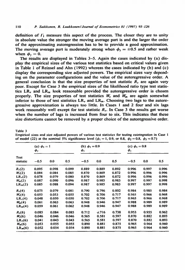
The results are displayed in Tables 3-5. Again the cases indicated by (a) display the empirical sizes of the various test statistics based on critical values given in Table 1 of Reinsel and Ahn (1992) whereas the cases indicated by (b) and (c) display the corresponding size adjusted powers. The empirical sizes vary depend- ing on the parameter configurations and the value of the autoregressive order. A general conclusion is that the size properties of test statistic Rv are again very poor. Except for Case 3 the empirical sizes of the likelihood ratio type test statistics LRv and LRm look reasonable provided the autoregressive order is chosen properly. The size properties of test statistics Wv and Wm are again somewhat inferior to those of test statistics LRv and LRm. Choosing two lags to the autoregressive approximation is always too little. In Cases 1 and 2 four and six lags work reasonably well except for test statistic Rv. In Case 3 the results get worse when the number of lags is increased fi'om four to six. This indicates that these size distortions cannot be removed by a proper choice of the autoregressive order.

Table 3 Empirical sizes and size adjusted powers o f various test statistics for testing cointegration in Case 1 o f model (22) at the nominal 5% significance level (O! = !, 0.9, or 0.8, ~2 = 0.8, qb3 = 0.7)

(a) Ol = 1 (b) 01 = 0 . 9 ( e ) O! = 0.8

Test statistic --0.5 0.0 0.5 --0.5 0.0 0.5 --0.5 0.0 0.5

Rv(2) 0.095 0.098 0.099 0.889 0.889 0.892 0.996 0.997 0.996 Wt,(2) 0.084 0.084 0.085 0.870 0.869 0.872 0.996 0.996 0.996 LRv(2) 0.078 0.079 0.080 0.870 0.869 0.872 0.996 0.996 0.996 Win(2) 0.087 0.090 0.096 0.987 0.985 0.983 0.997 0.997 0.998 LRm(2) 0.085 0.088 0.094 0.987 0.985 0.983 0.997 0.997 0.998

Rv(4) 0.075 0.079 0.081 0.790 0.796 0.802 0.984 0.985 0.984 Wv(4) 0.053 0.053 0.055 0.702 0.706 0.717 0.965 0.966 0.968 LR~.(4) 0.048 0.050 0.050 0.702 0.706 0.7 ! 7 0.965 0.966 0.968 Win(4) 0.061 0.063 0.063 0.948 0.946 0.947 0.988 0.989 0.989 LRm(4) 0.059 0.061 0.062 0.948 0.946 0.947 0.988 0.989 0.989

Rv(6) 0.085 0.084 0.085 0.712 0.716 0.738 0.953 0.955 0.962 Wv(6) 0.046 0.046 0.046 0.565 0.581 0.597 0.870 0.882 0.893 LRv(6) 0.041 0.043 0.043 0.565 0.581 0.597 0.870 0.882 0.893 W,,,(6) 0.053 0.055 0.055 0.890 0.881 0.875 0.965 0.964 0.960 LRm(6) 0.052 0.054 0.054 0.890 0.881 0.875 0.965 0.964 0.960

P. Saikkonen. i~ Luukkoneni Journal o f Econometrics 81 (1997) 93-126 111

Table 4 Empirical sizes and size adjusted powers o f various test statistics for testing cointegration in Case 2 o f model (22) at the nominal 5% significance level (41 = I, 42 = !, 0.9, or 0.8, 43 = 0.7)

(a ) 4 2 = I ( b ) 4 2 = 0 .9 ( c ) 42----0.8

Test statistic --0.5 0.0 0.5 --0.5 0.0 0.5 --0.5 0.0 0.5

Rv(2) 0.115 0.123 0.124 0.31 ! 0.339 0 2 8 2 0.872 0.882 0.870 W,(2) 0.085 0.092 0.091 0.321 0.362 0.317 0.871 0.884 0.882 LRv(2) 0.073 0.080 0.077 0.319 0.361 0.321 0.867 0.881 0.880 W'm(2) 0.095 0.095 0. i 07 0.438 0.503 0.447 0.925 0.935 0.935 LR,,,(2) 0.083 0.084 0.093 0.439 0.506 0.446 0.925 0.935 0.934

Rv(4) 0.138 0.141 0.151 0.312 0.316 0.294 0.796 0.805 0.808 Wv(4) 0.071 0.072 0.076 0.272 0.284 0.276 0.696 0.703 0.728 LRv(4) 0.060 0.062 0.063 0.270 0.283 0.273 0.688 0.696 0.720 W,,,(4) 0.073 0.072 0.075 0.406 0.432 0.420 0.822 0.828 0.832 LRm(4) 0.064 0.064 0.068 0.403 0.431 0.421 0.821 0.826 0.832

Rv(6) 0.195 0. ! 96 0.209 0.284 0.288 0.282 0.697 0.707 0.729 ;~,,(6) 0.069 0.073 0.081 0.225 0.235 0.223 0.507 0.518 0.534 LRv(6) 0.057 0.061 0.069 0.225 0.234 0.224 0.501 0.513 0.532 Win(6) 0.073 0.071 0.073 0.327 0.358 0.355 0.648 0.674 0.699 LRm(6) 0.064 0.062 0.065 0.327 0.357 0.354 0.647 0.672 0.697

As to the empirical powers in Tables 3-5, the general picture is very similar to that obtained from Table 2. In most cases the new test statistics W and L R . are more powerful than their competitors and often by a fairly wide margin. Test statistic Rv is most powerful in some cases but its poor size properties make this result rather meaningless, at least from a practical point o f view. In Case 3(c) test statistics Wv and LRv are sometimes more powerful than the new test statistics Wm and LR,,, but their superiority is not great.

5. Conclus ion

This paper has studied various test procedures which can be used for testing the cointegrating rank in infinite order VAR processes. The associated asymptotic d i s t r i b u t i o n t h e o r y w a s o b t a i n e d b y w e a k e n i n g p r e v i o u s a s s u m p t i o n s o f t h e r e l a -

t i o n between the sample size and selected order o f the V A R process. Some o f the considered tests were straightforward extensions o f previous l ikel ihood ratio tests or their c lose analogs obtained for finite order Gaussian V A R processes. In addition to these extensions s o m e entirely n e w tests were also deve loped for

112 P. Sa i kkonen . 17,. LuukkonenlJournal o f Econometrics 81 ( 1 9 9 7 ) 9 3 - 1 2 6

Table 5 Empirical sizes and size adjusted powers o f various test statistics for testing cointegration in Case 3 o f model (22) at the nominal 5% significance level (01 = 02 = I, 03 = 1, 0.9, or 0.8)

(a ) 03 = i (b ) 03 = 0.9 ( c ) 03 = 0 . 8

0"~ 0~ 0~

Test statistic --0.5 0.0 0.5 --0.5 0.0 0.5 --0.5 0.0 0.5

Rv(2) 0.190 0.160 0.374 0.355 0.273 0.582 0.887 0.831 0.998 W~.(2) 0.130 0.104 0.235 0.374 0.270 0.579 0.884 0.80 i 0.996 L R , ( 2 ) 0. 100 0.080 0.195 0.372 0.270 0.570 0.875 0.790 0.994 Win(2) 0.135 0.I 14 0.258 0.468 0.324 0.590 0.926 0.837 0.950 LR , , ( 2 ) 0. 110 0.090 0.222 0.464 0.322 0.584 0.922 0.832 0.948

Rr(4) 0.274 0.265 0.341 0.297 0.273 0.600 0.760 0.766 0.993 W~(4) 0.106 0.100 0.109 0.262 0.232 0.470 0.635 0.613 0.933 LRv(4) 0.081 0.077 0.082 0.260 0.232 0.466 0.624 0.603 0.927 W,n(4) 0. ! 10 0. ! 07 0.122 0.332 0.275 0.496 0.724 0.659 0.864 LRm(4) 0.086 0.089 0. 100 0.330 0.273 0.490 0.715 0.651 0.859

Rv(6) 0.420 0.409 0.465 0.294 0.246 0.535 0.647 0.675 0.978 W,(6) 0.125 0. I24 0.119 0.187 0.182 0.343 0.425 0.427 0.748 LRv(6) 0.094 0.091 0.090 0.189 0.183 0.338 0.421 0.422 0.733 Win(6) 0.127 0.129 0.130 0.250 0.218 0.372 0.515 0.472 0.674 LRm(6) 0.105 0.105 0.107 0.248 0.217 0.368 0.506 0.465 0.666

models with intercept terms included in the cointegrating relations. A limited simulation study was performed to investigate the finite sample properties o f the considered tests. The main findings o f this simulation study were the fol lowing.

( i ) The l ikel ihood ratio type tests had better size properties than their asymptotically equivalent alternatives. However, our results also indicate that one can always find cases where even these tests have problems with their size. In particular, it is possible that the null hypothesis is rejected quite too frequently.

( i i ) The test based on the approach used in Saikkonen ( 1 9 9 2 ) had severe size problems so that tests o f this type are not recommended for general use.

( i i i ) The new tests developed in the paper were generally more powerful than their competitors. Quite often their superiority was considerable although there were cases where the power o f the new tests and their previous alternatives was about the same.

Mathemat i ca l appendix

We shall make use o f results already employed in Saild<onen (1992, 1995) and Saikkonen and Lfitkepohl (1996) . Some o f them have been derived by assuming

P. Saikkonen, 1~ LuukkonenlJournal of Econometrics 81 (1997) 93-126 113

the lower bound condition (13). When these results are applied it will be under- stood that they are valid without the lower bound condition even i f this is not always explicitly mentioned. Since some of the subsequent derivations are rather long and tedious they will not be given in full detail. A more detailed treatment is available upon request. Before proving Theorem 3.1 some general remarks, also relevant for other proofs, will be made.

First recall that we can assume throughout that the triangular error correction form is as in (3). Unless otherwise stated, it will be assumed that all partitions of vectors and matrices are conformable to that o f yt in (1). The notation Bi.y = B ~ i - BoBj~tByi is used for any positive-definite matrix B = [Bij]i,j=l,2. The symbol H" [[ is used for the Euclidean norm so that, for an arbitrary matrix B, IIBII = [tr(B'B)] !/2. By IIBII, we mean the operator norm of the matrix B, that is, the square root o f the largest eigenvalue of B'B. These norms are connected by the well-known inequality

lIB,B211 ~ liB, II lIB211, (A.1)

which holds for any conformable matrices Bl and B2. The transformation matrix

,.] will be employed in several places. For instance, we have

= ÷ a -~ = [÷ , ~ 2 ] (A.2)

where ---@2 = q'IA_A_ + @2. Furthermme, under the conditions o f Theorem 3.1,

tJ~'l -- ¢i~ 4- op (K- I/2 ) (A.3)

-~--~2 -- Op( T - ! ) (A.4)

and

,~ -- ~' -4-op(K -1 ) (A.5)

(see Lemma A3 and the proof o f "~hc, Jrem 3.1 o f Saikkonen, 1995). If the lower bound condition (13) is assumed ~ahe order terms in (A.3) and (A.5) can be improved to Op((K/T) 1/2) and Op,[T-l/2), respectively [see Theorem 3.2 and result (A.14) in Saikkonen (1992) :and Theorem 3 o f Saikkonen and Lfitkepohl (1996)]. Analogs of ( A . 3 ) - ( A . 5 ) ere also valid when obtained fi'om the least squares regression (14) which incl~les an intercept (see Saikkonen, 1995).

P r o o f o f Theorem 3.1. Denote

9 = [E~]~j=,,2 = ÷ ' ~ - ~ ~'

114 P. Saikkonen. IL Luukkonen lJourna i o f Econometrics 81 (1997) 93-126

and note that ,~1 ~< " '" ~< 2",, are the e igenvalues o f the matrix C v. The matrices C and 17 are t rans tbrmed as

(7 = [__C,~]i.j=t.2 = A C A ' and I2 = [__##]i.j=l.2 = ___~,~-1__~

where ~ is as in (A.2) . This t ransformation does not change eigenvalues so that the matr ices C V and C # have identical eigenvalues.

We shall first consider asymptot ic properties o f the matr ix (7. F rom the definitions it fol lows that C = M -- G where

G = [Gi j ] i . j=l ,2 = ~ u l , t - ! , t t=K+2 Y2, , - , x, ~ , x, xtt ~ xt tu~.t_, Y2.t- t] t = K + 2 t = K + 2

and M = [Mij] i . /=L2 = A M A ' is the matr ix o f sums o f squares and cross products o f the components o f [ U i , t _ i t Y2,t--lt y ( t = K + 2, . . . , T). By (2) we have

A y t = A - I [ A u l t ] " - u2t

Therefore,

xt = Hqt

where qt = [ u ~ _ 1

observable) t ransformation matr ix o f full row rank. Denote

T T Sqq = N - ' E q,q~ and S,q = N - ' ~E ", . , - ,qL

t = K + 2 t = K + 2

Then, i f ~rqq =Eqtq~ and 2~lq - - E u l . t - l q ~ , we have

[ISqq - - Z~,qq ][I - - OP ( u / r l / 2 )

and

. . . U ¢ U t t -K l . t_K_t] ~ and H ( n K x ( n K + n l ) ) is a suitable (un-

(A .6)

l lS|q - - ~,lq [[ = O p ( ( g / T ) l / 2 ) . ( A . 7 )

These results can be obtained from the p roof o f L e m m a A.2 o f Saikkonen (1991 ). In the same way one also obtains

Ii II IIS2qtl ~f N - ' ~ Y2, t - - lq~ = O p ( ( l / 2 ) - (A.8) t = K + 2

Now, we can study asymptot ic properties o f the matrix (7. We start with mull and observe that

N - ! Gt i -- S tqH ' (H~ ,qqH' ) - I HS~q

= - - S l q H ' ( H ~ q q H ' ) - 1H[Sqq -- ~qq]Ht(HSqqH ' ) - i HS;q. (A.9)

P. Saikkonen, R. LuukkonenlJournal of Econometrics 81 (1997) 93-126 115

Our assumptions imply that the eigenvalues of the matrix ~E~ are bounded and bounded away from zero. Hence, from Lemma A.2 o f Saikkonen and Lfitkepohl (1996) it follows that an analog of (A.6) also holds for the corresponding inverses and, from Lemma A. l o f the same paper, one therefore obtains

IIH'(HZqqH')-~HIIE = O(I) and IIH'(HSqqH')-IHIll = Op(1). (A.|0)

Furthermore, since the covariance function of u, is absolutely summable, [[Z'lq[[ is bounded uniformly in K and it follows from (A.7) that

llSlq II - op( l ). (A. l X)

Now, using (A.10) and (A.II) in conjunction with (A.6) and (A.I) one can see that the Euclidean norm of the fight-hand side of (A.9) is of order Op(K/Tl/2)--Op(1). From (A.7) it similarly follows that the error of replacing S~q by Z1q in the second term on the leR-hand side of (A.9) is of order Op(1). Finally, by the law of large numbers, N-IMIj =Etll,t_lu t l , t -! + Op(l) SO that, since C 1 ! -- M_M_ ! ! -- Gi i, we can conclude that

: U t -- ~ l q H ' ( H ~ , q q H t ) - l H ~ q ":t- op(l) . (A.12) N-IC--ll EUl,t-! i , t -!

The two first terms on the right-hand side o f (A.12) define the covariance matrix o f the prediction error obtained by linearly predicting ul,t--! by Hqt or, equivalently, by xt. The same prediction error is obtained by linearly predicting u~,r-i by {Au l , t - j , u2,t-j, j "- 1 . . . . . K}. As K--~ oo, the smallest eigenvalue o f the covariance matrix o f this prediction error must be bounded away from zero since this is the case for Eqq, the covariance matrix o f the random vector qt = [u,_' l . . . utt_K utl , t_r_l ]'. Hence, we have shown that, with a probability approaching one,

N - I C l l >~Int, ~ > 0. (A.13)

Since N - I G l 2 - - S l q H ' ( H S q q H ' ) - I H S ~ q arguments similar to those used to ob-

tain (A.13) can also be used to show that N - I G 1 2 : O p ( K l / 2 ) . Hence, since N-IM___12 - -Op( l ) [see Saikkonen (1992, p. 26)] and C i e -----Ml2 + Gl2, we have

N - I C I 2 : Op(gl/2) . (A.14)

From N -2 G22 = N - 1SzqH'(HSqqH')- ! H S ~ it similarly follows that [ IN-2G~ [[ -- Op(K/T) . Thus, i f we partition M--[Mij]i , j=l ,2, we have M2z =Mgz and

N-2CC22 -- N-2M22 -{- Op((g /T) !/2 ). (A. 15)

Here the error term could be Op(K/T) but the above result will be convenient in the proof o f Theorem 3.3.

The limiting distribution o f test statistic W can now be derived by using the above results and arguments similar to those in the proof o f Theorem 4.1 o f

116 P. Saikkonen, R. LuukkonenlJournal o f Econometrics 81 (1997) 93-126

Saikkonen (1992). First notice that ~l ~< "'" ~<~n are the eigenvalues o f the matrix C ~" in the metric X and

From (A.3), (A.4), (A.14) and (A.15) one obtains N-I~CW I = N - - l ~ i C l l ~ + Op(1). Hence, using (A.3) , (A.12) and (A.13) we can show that, with a probabil-

ity approaching one, the n i largest eigenvalues o f N -m V'C ~ ' are bounded and bounded away from zero. Noticing (A.5) we can thus conclude that ~.y, j = n2 + 1 . . . . . n, tend to infinity at the rate Op(N). Let O_L(n X n2) be a matrix such that ~ _ O ± = I,,~ and ~'L W! ---0. Then, since N - 2 M 2 2 converges weakly to a matrix which is positive definite (a.s.) [see (A.10) in Saikkonen (1992)] we can use (A.4) and (A.15) to show that q~ WC ~"O_L = Op( l ) . This result and the Poincare separa t io . theorem (see Rao, 1973, p. 64) imply that ) V - Op( l ), j - - 1 . . . . . n2.

In the san2e way as in the proof o f Theorem 4.1 o f Saikkonen (1992) we now consider ~.1 ~< "-- ~<~.~ as solutions o f the general ized eigenvalue problem [ P - - ) , C - I [ = 0 . Denote E_*(A)= [ff__~-j(g)] = ~ - A C - t and note that, when IETI(A)I

0, the equality 1F_*(A)I- 0 can be expressed as

IFT~(A)I IF~.~(),)I - 0.

Consider the nl solutions o f tFT,(A)I = 0 and notice that

F___* I I(3,) ----- @I,~-I @l -- :.CT.t2 -- /?l, -- :tCT-t~,

where /?ll--¢/2~--lqb + °p(I) by (A.3) and (A.5). From (A.14) and (A.15) it also follows that

-- N - ' C -+- O p ( K / T ) . N - 1 C t - 2 --11 (A.16)

Using this result, (A.12), and (A.13) one can show that the nl solutions o f I F ~ I ( A ) I = 0 tend to infinity at the rate Op(N). 5 N o w recall that we showed above that the n2 smallest solutions o f IF*(A) I - - 0 are o f order Op(1 ). There- fore, asymptotical ly they cannot solve IF_h(~.)l = 0 and we can consider ~.j, j = 1 . . . . . n2, as solutions o f IF_~.,(~.)I = 0 or, equivalently, [N2F~.I(A)[ = 0 . Fur- thermore, in the analysis below we can assume that A = O( I ).

By L e m m a A.2 o f Saikkonen and Liitkepohl (1996) the error terms in (A.15) and (A.16) do not change when the involved matrices are replaced by the corresponding inverses. This fact in conjunction with (A.13) and (A.14) shows that

5 N o t i c e that, unl ike s ta ted in Sa ikkonen (1999 , p. 26) , one cannot d i rec t ly conc lude from this that Aj = O p ( N ) , j : n2 + ! . . . . . n. A similar remark concerns the related p rev ious s ta tement abou t the smal les t e igenva lues Aj, j ---- 1 . . . . . n2. There fo re the present p r o o f differs f rom the p rev ious one at these points.

P. Saikkonen. R. Luukkonen/Journal o f Econometrics 81 (1997) 93-126 117

C_.-~C21C-~.~=Op(KI/2/T2). Thus, as A = O ( I ) can be assumed, we can use the definitions and the inversion formul~ of a partitioned matrix to obtain

= - = ÷ Op(f'/2/r2).

By similar arguments we also have F~l (A) = ~11--),C~.J = TY~ +Op(T - l ). Hence, Lemma A.2 of Saikkonen and Lfitkepohl (1996) gives

= + Op(Y ).

As for F~2(A ), it follows from (A.13)- (A.15) that N-2C2.t =N-2M22- [ - Op((K/T) 1/2 ) so that, using Lemma A.2 of Saikkonen and Lfitkepohl (1996) again,

F~2( '~) = ---.V22 -- ~C~.] = ----V22 -- ~ I r ~ i - I - o p ( T - 2 ) .

Thus, since ~2t -- . ~ - 1 ~ , - -Op(T - I ) and __VHI---(~J~-I~I)-I = O p ( l ) , we can conclude from the above discussion t ha t N2F~. I (~ , )=N2(__V2.1 - - , ~ [ 2 2 1 ) -[- op(l ). Hence, by the continuity of eigenvalues,

W --- t r ( M 2 2 ~ 2. I ) -~ Op( 1 ).

It was shown in Saikkonen (1992, pp. 26-27) that R=tr(M22/72.1)+ op(l) =~ ~(n2). Equation (A.30) of that paper implies that the same result is also obtained here because the previous definition of the matrix • is asymptotically equivalent to the present one and because the limiting dmtribution of the estimator ---~2 does not require the lower bound condition (13), as shown in the proof of Theorem 3.1 of Saikkonen (1995). Thus, test statistic W has the stated limiting distribution. The asymptotic equivalence of test statistics W and LR discussed below Theorem 3.1 follows from a standard mean value expansion of the logarithmic function. This completes the proof. []

Proof of Theorem 3.2. In the same way as in the proof of Theorem 3.1 we first transform the matrices ~v and C by using the transformation matrix A_ and obtain analogs of (A.3)- (A.5) . Next, using arguments in S~:.k~onen (1992, p. 22) it can be shown that analogs of (A .6) - (A.8) and furthermore (A.13)- (A.15) hold even in the present context. The proof can then be completed by using arguments entirely similar to those in the proof of Theorem 3.1 [cf. Saikkonen, 1992, p. 27). Details are omitted. []

Proof of Lemma 3.1. For simplicity, we shall assume the asymptotically negligible initial value conditions Y0 ---- 0 and vt -- 0, t ~ 0. For notational convenience the subscript v will be suppressed from the estimators B,j, ~, , /1~ and Z, and similarly from quantities derived from them. This should cause no confusion since we shall only use such properties of these estimators which are not affected by the inclusion of the intercept in the model.

118 P. S a i k k o n e n , R. L u u k k o n e n l J o u r n a l o f E c o n o m e t r i c s 81 ( 1 9 9 7 ) 9 3 - 1 2 6

The a s sumed initial va lue condi t ions imply that in (16 ) we have e t - - e t for t - - 1 . . . . , K + 1 whi le for t > ~ K + 2, et is as defined in (6) . Thus, replac ing B j

in (16 ) b y / } j ( j -- I, . . . , K + 1 ) g ives the regress ion equat ion

d , = C t m + et , t = 1 . . . . . T, ( A . 1 7 )

where

t - - I e.t -- ~ , ( B j -- B j ) Y t _ j , t---- 1 , . . . , K + 1

j=l K

et - - (t~.l _ t p ) y t _ l _ ~ ( [ l j - - r l j ) A y , _ j , j = l

t = K + 2 . . . . . T.

Set ~ , =[_~_,, ~ , 2 ] = C t A _ - ' and, as before, ~ = [~', initions and the above discussion we can then write

---~2] = @~-=- By the dot'-

A_(th -- m ) = ___.u-i~ ( A . I 8 )

where

K + !

and

[ ] T E

Next , we shall ana lyze the matr ix __U and start by cons ide r ing the quant i t ies __Cj, j = 2 . . . . . K + 1. Since ¢ ~ j = - ~ ' - / l j - ! we have C j I = -- ~ul - / l j - ~ , l and

~j2 = -----~2 --/~ry-,.z where H j 2 = Hj,A + Hi2. We also define / I , , = @= + HI , and l = l j t - - f l i t - l=lj_,.,, j - -2 . . . . . K. Then H__"- [_~_, ... / IK] , where H j -- [ ~ j l Rj2], is exact ly as in Sa ikkonen (1992, p. 19) except tbat the a symp- tot ical ly i r relevant restr ict ion /~rK! = 0 has not been used. (No te also the printing error in the p rev ious defini t ion o f / l j l - ) The theoret ical counterpar ts o f H j

and H_0_" are def ined in an obvious m a n n e r and deno ted by H j = [_H_jl Hj2] and F / = [_H_l . . . / / r ] , respect ively. By L e m m a A.3( i ) o f Sa ikkonen (1995 ) we have

II~- ~II = op(K-I/2) o (A .19 )

S ince l l j 2 = / / y t A +/-/j2 and Cj2 = -- ---~2 - - / I j - l , 2 ( J = 2 , . . . , K + 1 ) it is straight- fo rward to deduce f rom this that

K + I

:E II~j211 = Op(l). (A.20) j = l

P. Saikkonen, 1~ L u u k k o n e n l J o u r n a l o f Econometr ics 81 (1997) 93 -126 119

As for C j l , we first observe that

j - - !

~ j l = - - (~ l + / l j - i , t ) -- - - ~ H__- ~i, j -- 2 , . . . , K + 1, (A.21) i=l

where the latter equation follows from the definition o f the sequence l l j t . Argu- ments similar to those in the case o f (A.20) show that

max II--Cjl II = Op( i ). (A.22) l <_j<~K+!

Using the above results in conjunction with ( A . 3 ) - ( A . 5 ) it can now be shown that N-~___011 = ~ , ~ . - l ~ + op( l ) , __012 = O p ( l ) and ___022 = O p ( l ) . Furthermore, i f __0 - l = 10iJ]/j=l.2, these results and the inversion formula for a partitioned matrix yield

N~_U II -- (~t .E ' -140 - ! 4 - % ( 1 ) (A.23)

0___ 22 = Op( i ) (A.24)

and

__012 -- O p ( N - 1 ). (A.25)

To analyze the asymptotic behavior of the vector ~ an order o f consistency is needed for the estimator B - [ / ~ I . . . Blc]. As is (A.2) o f Saikkonen and Lfitkepohl (1996), define ~,'-L_H_ / /KI] and "~ - = - L~_- H K,, ], and note that I1~- Sll =Op(K'--1/2), by Lemma A.3(i) o f Saikkonen (1995). From the proofs o f Theorems 1 and 2 of Saikkonen and Lfitkepohl (1996), one also obtains

B -- B - - ( ~ -- S ) P I 4- Z where B - - [ B I . . . BK], IlZll---~Op(N-I), and Pi is a nonstochastic matrix ~ach that IlPa ill =O(1). Thus, making use o f (A . I ) , we find that

l i b - BII = (A.26)

Using this result and wel l -known properties of integrated processes it is straightforward to show that

1 <<.t~K+! j = !

This result can be used to analyze the residual ~t for t---- I , . . . , K 4- 1. For other values of t we shall use the representation

e t ' - e t - - ~ _ _ 2 Y 2 . t - l - - ( ~ - - ~ - ~ ) q t , K + 2 . . . . ,T, (A.28)

which can be obtained from the earlier definition o f et with transformations similar to those above (A.19) [of. (A.2) of Saikkonen (1992)]. Now, from (A.28)

1 2 0 P. Sa ikkonen , !~ L u u k k o n e n l J o u r n a l o f Econometr i c s 81 ( 1 9 9 7 ) 93-126

and the definitions of ~1 and ~, it follows that

= _ C t t ~,-I y~. -- B j ) Y t - j t= 1 t= 1 j = 1

+ +

(A.29)

where e, fi2 and ti are the sample means of et, y2 . t - i and qt ( t = K + 2 , . . . , T ) , respectively. Using of (A.5), (A.22) and (A.27) it can be shown that the first and second terms on the right-hand side of (A.29) are of order Op(I ). From the definition of et below (6) and well-known properties of stationary processes it follows that ~ : O p ( T - l / 2 ) . This result in conjunction with (A.3) and (A.5) implies that the third term on the right-hand side of (A.29) is of order Op(l) . Next note that -v2 =Op(TI/2) and I I~][=Op((K/T) !/2) (see Saikkonen 1992, pp. 21-22). Hence, since II~-_=ll--op(K-l/2), it follows from ( A . 3 ) - ( A . 5 ) t h a t the fourth and fifth terms on the right-hand side of (A.29) are of orders Op( l ) and op(l ), respectively. As a whole we have thus shown that

T-I/2~ ! -- Op(l) . (A.30)

Next, con~ider

K + l K + I t - - I T

t = 1 t = I j = 1 t = K + 2

(A.31)

The analysis given for the last three terms on the right-hand side of (A.29) readily shows that the third term on the right-hand side of (A.31) is of order op( l ) while the second one is of order op(K !/2) by (A.5), (A.20) and (A.27). Finally, since ~t2 = -----~2- / I t - l ,2 for t = 2 , . . . , K + 1, we can use (A.4) and (A.19) to show that the first term on the right-hand side of (A.31) is of order Op(l) . Thus, we have

h_-2 = op(K !/2). (A.32)

From (A.18) one now obtains O ' ( ) h - m)=O__llh_ I + _U_Ul2~2--Op(r-l/2 ) and J_~(m- m)---__U21h_'!-~-U____22~2 =Op(Kl/2 ) where the order terms are justified by (A.23) - (A.25) , (A.30) and (A.32). This completes the proof. It may be noted, however, that if the lower bound condition (13) is assumed we have H~, - 3,[] - - O p ( ( K / r ) 1/2) (see Saikkonen (1992, pp. 20-21) and the right-hand side of (A.26) can be changed to Op((K/T) l /2 ) . This implies that the right-hand side of

P. S a i k k o n e n , IL L u u k k o n e n l J o u r n a i o f E c o n o m e t r i c s 81 ( 1 9 9 7 ) 9 3 - 1 2 6 121

(A.27) can be improved to O p ( ( K 3 / T ) l / 2 ) = o p ( l ) and we have h" 2 = O p ( l ) . The latter result o f the lemma can thus be improved to J_~(n~ - - m ) = Op( l ) . []

Before proving Theorem 3.3 an auxiliary result will be given. First note that ~ s and/Tm are ordinary least-squares estimators obtained from the model

Azt -" ~ f ' t - ! + l l x t + at, t = K + 2 , . . . , T, (A.33)

where Yt-~ = z t - t - t~ and a t : e t -t- t~Ot( t~t - - m ) . Set

. [.,,] Y2t L Jr-( ~ -- m ) = fii2t "

In the same way as in (A.28) we can transform (A.33) to

Azl = ---~2.P2,t-i + ~q, + at, t = K + 2 . . . . . T, (A.34)

where 9' 2 OA + q~z O, #, [~?~t q~,]' with ~]tt " - " ' = = = = [ u l , , _ ! . . u l , , _ r _ l ] , and q2t----[u2,t_l . - . U2,t_K]. The coeff ic ient mat r i x -- is def ined in the same w a y as in t h e p r o o f of Lemma 3.1 except for an irrelevant permutation o f columns. Let ~m and ---~,,,2 be the (infeasible) least squares estimators of = and _~2,respectively, obtained from (A.34). As in Saikkonen (1992, p. 18) we then have 9",,2 = tP,,,O± where O L = [.4' In.]L

Next, consider an analog of (A.34) defined by

A z t = q J 2 y 2 , t - l + ~ . q t + e t , t = K + 2 . . . . . T, (A.35)

! . . . 1~ t 11 where now qt =[q~t q~t]' and q l t =[Ul,t--I I , t - - K - - l J " Thus, (A.35) is derived from (6 #) in the same way as (A.34) is derived from (A.33). Let ~ and ---~2 be the least-squares estimators of S and qJ2, respectively, obtained from (A.35). Then 9"2 = tPO-L where ~' is now the least-squares estimator of qJ obtained from ( 6 " ) with m treated as known. Now we can prove following.

L e m m a A. 1. U n d e r t he c o n d i t i o n s o f T h e o r e m 3.3,

T

N~_.m2 ~- N~___. 2 + ~ 0 ' ( ~ - m ) N - ' ~_. Y~ , t - , t = K + 2

x Y 2 , t - l Y 2 , t - t d- Op(l) 2

~',nl = • + op(K -1/2)

a n d

£,m = Z + o p ( K - t ).


Proof . Denote fit =[t]~ ,P[. t- l] ' and /lm--'[~m --~--~m2] and note ,hat

T T )--1 (/Zm -- A ) D r ! = ~ a t f f t D r ( D r ~ p t f f t D r , (A.36)

t=K+2 ~ t=K+2

where A = [ ~ ~ ' 2 ] = [ S 0] and D r = d i a g [ N - n / 2 1 n X + n , N - ! In2]. We shall consider replacing /5 t in (A.36) by Pt [q~ ' ' = Y2. t - ! ] - We can write

qlt = ~ " -- (z ® O ' ) ( ~ -- m) and f'et = Y2t -- J~_(,'n -- m) ,

where z ----[1 --- I ] ' ( ( K + 1) x 1). Recall that the sample means o f qt and Y2,t-t (t----K + 2 , . . . , T ) are o f orders O p ( ( K / T ) 1/2) and Op(Tl/2) , respectively, while [ ] ( t ® O ' ) ( , ' ~ - m ) l l = O p ( ( K / T ) t/2) and ( l f i - m)d_t_=op(K 1/2) by L e m m a 3.1. Using these results it is straightforward, though somewhat tedious, to show that

I I T T II Pt f f D r -- D r _~+2 Pt p [ D r = O p ( ( K / T ) !/2). Drt=~r + 2 (A.37)

ii _, a,q, ll ,:2, Furthermore, by L e m m a 3.1 and the result # = Op(T- l / 2 ) ,

T T N -l ~ "t N-I ,

atY2, t - - i Y~ 1 -- e tY2, t - -- O 0 ' O f i -- m ) f ~ t=K+2 t----K+2

= --~(r~ -- m) ' J± -- ~ 0 ' ( ~ -- m)(tf i -- m) ' J±

-- Op((K/T) l /2) .

(A.40)

(A.41)

Next note that

T T

t=K+2 t=f +2

- -Nl /2~(t~ -- m ) ' ( d ® O ) -- N I / 2 ~ O ' ( r ~ -- m)( t~ -- m ) ' ( d ® O ) (A.38)

where ~ is the sample mean o f qlt ( t = K + 2 , . . . , T ) . Using arguments similar to those referred to above one can here show that the norm o f the left-hand side is o f order O p ( ( K / T ) 1/2) and that the same result holds with t]! t and qlt replaced by q2t. Hence, it follows that

r ,,= ,(-, .ll N -~/2 ~ at#~ -- N- (A.39) = OP((K/T)'/2)"

From the definition o f et given below (6), (A.7) o f Saikkonen (1992) , and L e m m a A.2(i i ) o f Saikkonen (1995) we can conclude that the Euclidean norm of the latter matrix on the left-hand side o f (A.39) is o f order Op((T/K) l /2) . Thus, (A.39) yields

P. Saikkonen, R. Luukkonen/ Journal of Econometrics 81 (1997) 93-126 123

Denote

T Dr ~ pip, Dr = R = [Rij],j=t,2 and R - ' = [Rqli, j=l,2,

t=K+2

where the partitions are conformable to that of P t - [q[ ' y2.t_l] ~. Lemma A.I of Saikkonen (1995) gives IIR'211, ----Op((K/r) '/2) and R 22 - -Op( l ). Thus, using (A.36) - (A.38) it readily follows that

T T N~_~_.m2 :- N -I/2 ~ atqttf~ 12 -[- N -I Y~ atf,,t2,t_l R22 -+- op(l). (A.42)

t=K+2 t=K+2

The first term on the right-hand side is of order op(l ) by (A.40) znd the above- mentioned result lira2111 = Op((g/T)l/2). Hence,

N~_.m2 N - I ~-~ ' N - ~ ' "-" etY2,t--! Y2, t - - lY2, t - i t~K-t-2 t~-K+2

2 T )--1 - t-~O'(t~ -- m)f,~ N- ~_, Y2,t-,Y~,,-I

t=K+2 + Op(l )

where we have made use (A.41) and Lemma A. l ( i i i ) of Saikkonen (1995) which justifies the replacement of k 22 by the indicated inverse. Lemma A.2(i) of the same paper implies that in the last expression it is further possible to replace et by et. The first assertion of the lemma follows from this and the discussion in Saikkonen ( 1992, pp. 20-21 ).

To prove the second assertion, first note that (A.21) and the definition of the matrix ~, (see below (A.25)) give

K+I

j=l

where the matrix JK = [ - J ' . . . - - J ' In,]' ( (Kn + nl ) × n l ) has the property iIJxlll = ( K + l y/2. Similarly, O--- =~EJK and therefore @l - O = ( ~ m - ~=)Jx- From (A.36) and arguments similar to those used to analyze (A.42) it now follows that

T @l -- ¢~ : N - I ~ atqttelljK 4" O p ( ( K / T ) l / 2 ) .

t=K+2

Recall that £,qq = Eqtq't and note that [[/~ll _Z~ql Ill = Op(K/TI /2 ) by Lemma A. l ( i ) of Saikkonen (1995). From this result, (A.39) and (A.40), one obtains

T - = E e, Z q'J c + op(g/rl/2).

t=K+2


The arguments given in the proof of Lemma A.3 o f Saikkonen (1995) show that the last expression is of order op(K- l /2) , as required.

As to the third assertion, its proof is very similar to that o f Lemma A.3(ii i) o f Saikkonen (1995), so only a br ief outline will be given. First note that [ [ A m - All = op(K - I /2) by the derivations in the proof o f the first assertion o f the lemma. Then observe that eT,,,t -- at -- (fi-m -- A).bt so that arguments similar to those in the above-mentioned previous proof show that in the definition of Zm the replacement o f ~mt by at causes an error which is of order op(K - ! ). Next, since at = et + O O ' ( t h - m), one can use Lemma 3.1 to show that a t can further be replaced by e t . After this, it suffices to use an argument already given in the proof of Lemma A.3(ii i) o f Saikkonen (1995). []

P r o o f o f T h e o r e m 3.3. Following the proof o f Theorem 3.1 we first define

= [~ij]i , j=l .2 = A C A ' a n d --~-Vm - - [V___m.ij]i.j=l,2 = l~//m'~ml_~_~m,

where ---~m = [~,,,' ---~m2] = tPmA---t" Then ~-ml ~ < " " ~< 2m, are the eigenvalues o f the matrix ~ #m" The mairix C can tm written as C ' = M - - ( ~ where M___-- [M___,•]ij=l.2 and ( ~ = [Gij]i,j=l,2 are defined by replacing u l . , - t and Y2.t-I in the definitions o f M and G by ~l,t-1 and fi2,t-t, respectively (see the beginning of the proof o f Theorem 3.1). Using 171.t--I and .P2,t-t we similarly define analogs of the ma-

trices Sqq, Stq and S2q and denote them by Sqq, Slq and S2a, respectively. Then, using (A.38), (A.40) and Lcmma 3.1 it can tm shown that ( A . 6 ) - ( A . 8 ) also hold with Sq¢, Slq and S2q replaced by Sqq, S iq and S2q, respectively. By similar arguments it can further tm seen that the matrices M and M are related as N-IM---- li = N-tM---! l + op( l ) , N-tm___~ t2 = N - I m l 2 -- O ' ( rh - -m) f i t2 + Op(1) = Op( l ) and N-2M____" 22 = N-2M_M_22 + Oo((K/T) I /2) . Using the above results we can now re- peat the derivations used to prove ( A . 1 2 ) - ( A . 1 5 ) and show that these results also hold with C~j replaced by ---Co"

Now, the proof proceeds in the same way as that of Theorem 3.1. The first step is to consider ~.mi ~ " - " <.~ Amn as eigenvalues of the matrix ---~m C___~ m " ~' in the metric ,~,~ and show that 2mj, j = n2 + l , . . . , n , tend to infinity at the rate Op(N) whereas ) . m j = O o ( 1 ) for . ] = 1 , . . . ,n2 . Here analogs of ( A . 3 ) - ( A . 5 ) obtained from Lemma A.I are used in addition to the above-mentioned results. Next, d e n o t e E ( ~ L ) = ~ _ i j ( A ) ] i . j = l , 2 =-~--Vm- , ~ - , - t and use Lemma A.I to show that ---#m, I I = ~,Z--! ~ + Op(l ). In the same way as in the proof o f Theorem 3.1 one can then show that the ni solutions of IF__" lk(A)l = 0 tend to infinity at the rate Op(N). Thus, the n2 smallest eigenvalues of C V m solve [N2~2.1(2)l = 0 where N 2 ~ 2 . 1 ( 2 ) = N 2 ( f ' m , 2 . i -- ,;al4~ l ) + Op(1) by arguments similar to those in the proof o f Theorem 3.1. Note that the only property o f the (infeasible) estimator ---~m2 we have so far needed is ---,~m2--Op( N - I ). To complete the proof we also

P. Saikkonen, R. Luukkoiwn/ Journal o f Econometrics 81 (1997)93-126 125

need the representation provided in Lemma A.I. First, in the same way as in (A.30) o f Saikkonen (1992) we can use the definition o f #_~ to obtain

N2V___~,2., - - N2_~_.~2Q._~m2,

where Q - - ~ ' - E~' qJ~,(-' ~ m ' ~ t ~/'~t ~' )--'. ~-- ~ , t . Let Q be the analog o f Q defined by using E and • in place o f Zm and ~'ml, respectively. From Lemma A.1 we can then conclude that Q = Q + Op(l ) a n d , since Q O = 0, also that

2 " ! - ~ N tllm2Q~___.m 2 = N 2 _~Q,.~_~2 -~- Op( l ), H e n c e

~m = tr(J~f22_~Vm,2.1 ) ~t- Op( 1 ) = t r (~f22 ~.....t2Q___.~ 2) -~- Op( 1 ),

As discussed in the proof o f Theorem 3.1, the limiting distribution o f the estimator ---~2 is here the same as in Theorem 4.1 o f Saikkonen (1992) and the previous definition o f the matrix • is asymptotically equivalent to the present one. The arguments given in Saikkonen (1992, pp. 2 6 - 2 7 ) thus show that the first term in the last expression converges weakly to ~(n2). This completes the proof. []

References

Anderson, T.W., 1951. Estimating linear restrictions on regression coefficients for multivariate normal distributions. Annals of Mathematical Statistics 22, 327-351.

Beck, K., 1974. Consistent autoregressive spectral estimates. The Annals o f Statistics 2, 489-502. Elliot, G., Rothenberg, T.J., Stock, J.H., 1996. Effmient tests for an autoregressivc unit root.

Econometrica 64, 813-836. Engle, R.F., Granger, C.W.J., 1987. Cointegration and error correction: Representation, estimation

and testing. Econometrica 55, 251-276. Johansen, S., 1988. Statistical analysis o f cointegration vectors. Journal of Economic Dynamics and

Control 12, 231-254. Johansen, S., 1991. Estimation and hypothesis testing of cointegration vectors in Gaussian vector

autoregressive models. Economelcica 59, 1551-1581. Johansen, S., Juselius, K., 1990. Maximum likelihood estimation and inf=~c,K:e on cointegration - with

applications to the demand for money. Oxford Bulletin of Ec,momics and Statistics 52, 169-210. Lewis, R., Reinsel, G.C., 1985. Prediction of multivariate time series by autoregressive model fitting.

Journal of Multivariate Analysis 16, 393-411. Ng, S., Pert'on, P., 1995. Unit root tests in ARMA models with _ ~ _ ~ ~ t methods for the

selection of the truncation lag. Journal o f the AJnnc'dcan Statistical Association 90, 268-281. Pantula, S.G., Gonzales-Fari¢% G., Fuller, W.A., 1996. A comparison of unit root test criteria. Journal

o f Business & Economic Statistics 12, 449-459. Phillips, P.C.B., 1991. Optimal inference in cointegrated systems. E c ~ 59, 283-306. Phillips, P.C.B., Ouliaris, S., 1990. Asymptotic properties of residual based tests for cointcgratkm.

Economctrica 58, 165-193. Rao, C.R., 1973. Linear Statistical Inference and Its Applications, 2rid od. Wiley, New York. Reinsel, G.C., Ahn, S.K., 1992. Vector autoregressive models with unit roots and reduced rank

structure: Estimation, likelihood ratio test, and forecasting. Journal o f Time Series Analysis 13, 353-375.

126 P. Saikkonen. 1~ LuukkonenlJournal o f Econometrics 81 (1997) 93-126

Said, S.E., Dickey, D.A., 1984. Testing for unit roots in autoregr,:~sive-moving average models of unknown order. Biometrika 71, 599-607.

Saikkonen, P., 1991. Asymptotically efficient estimation of cointegration vectors. Econometric Theory 7, 1-21.

Saikkonen, P., 1992. Estimation and testing of cointegrated systems by an autoregressive approximation. Econometric Theory 8, 1-27.

Saikkonen, P., 1995. Estimation and testing in infinite order cointegrated vector autoregress.ive processes with data-dependent choice of the truncation lag. Manuscript, University of Helsinki.

Saikkonen, P., L~tkepohi, H., 1996. Infinite order cointegrated vector autoregrcssive processes: Estimation and inference. Econometric Theory 12, 814--844.

Schmidt, P., Phillips, P.C.B., 1992. LM tests for a unit root in the presence of deterministic trends. Oxford Bulletin of Economics and Statistics 54, 257-287.

Stock, J.H., Watson, M.W., 1988. Testing for common trends. Journal of the American Statistical Association 83, 1097-1107.

Yap, S.F., Reinsel, G.C., 1994. Estimation and testing for unit roots in a partially nonstationary vector autoregressiv¢ moving average model. Journal of the American Statistical Association 90, 253-267.

Testing cointegration in infinite order vector autoregressive processes

Documents