Testing coherent reflection in chinchilla: Auditory-nerve responses predict stimulus-frequency emissions Christopher A. Shera a Eaton-Peabody Laboratory of Auditory Physiology, Massachusetts Eye and Ear Infirmary, 243 Charles Street, Boston, Massachusetts 02114 and Department of Otology and Laryngology, Harvard Medical School, Boston, Massachusetts 02115, USA Arnold Tubis Department of Physics, Purdue University, West Lafayette, Indiana 47907 and Institute for Nonlinear Science, University of California, San Diego, La Jolla, California 92093, USA Carrick L. Talmadge National Center for Physical Acoustics, University of Mississippi, University, Mississippi 38677, USA Received 3 December 2007; revised 7 April 2008; accepted 8 April 2008 Coherent-reflection theory explains the generation of stimulus-frequency and transient-evoked otoacoustic emissions by showing how they emerge from the coherent “backscattering” of forward-traveling waves by mechanical irregularities in the cochlear partition. Recent published measurements of stimulus-frequency otoacoustic emissions SFOAEs and estimates of near-threshold basilar-membrane BM responses derived from Wiener-kernel analysis of auditory-nerve responses allow for comprehensive tests of the theory in chinchilla. Model predictions are based on 1 an approximate analytic expression for the SFOAE signal in terms of the BM traveling wave and its complex wave number, 2 an inversion procedure that derives the wave number from BM traveling waves, and 3 estimates of BM traveling waves obtained from the Wiener-kernel data and local scaling assumptions. At frequencies above 4 kHz, predicted median SFOAE phase-gradient delays and the general shapes of SFOAE magnitude-versus-frequency curves are in excellent agreement with the measurements. At frequencies below 4 kHz, both the magnitude and the phase of chinchilla SFOAEs show strong evidence of interference between short- and long-latency components. Approximate unmixing of these components, and association of the long-latency component with the predicted SFOAE, yields close agreement throughout the cochlea. Possible candidates for the short-latency SFOAE component, including wave-fixed distortion, are considered. Both empirical and predicted delay ratios long-latency SFOAE delay/BM delay are significantly less than 2 but greater than 1. Although these delay ratios contradict models in which SFOAE generators couple primarily into cochlear compression waves, they are consistent with the notion that forward and reverse energy propagation in the cochlea occurs predominantly by means of traveling pressure-difference waves. The compelling overall agreement between measured and predicted delays suggests that the coherent-reflection model captures the dominant mechanisms responsible for the generation of reflection-source otoacoustic emissions. © 2008 Acoustical Society of America. DOI: 10.1121/1.2917805 PACS numbers: 43.64.Jb, 43.64.Bt, 43.64.Kc BLM Pages: 381–395 I. INTRODUCTION Most cochlear models represent the material properties of the cochlear partition by smooth and continuous functions of position. For example, to match trends in physiological data relating characteristic frequency to position, model pa- rameters are varied so that the stiffness of the basilar mem- brane BM decreases exponentially from base to apex. But although continuity and smoothness can be realized in math- ematics, the cochlea is a biological device assembled from discrete cellular components, each subject to developmental noise and other morphological aberrations e.g., Finch and Kirkwood, 2000. Standard assumptions about smoothness certainly simplify the model equations, but real cochleae must be mechanically irregular. How does mechanical irregularity affect cochlear model responses to sound? Simulations and analysis based on the application of Newton’s laws have answered this question in active cochlear models: The major functional consequence of modest mechanical irregularity in the organ of Corti is the production of long-latency evoked and spontaneous otoa- coustic emissions e.g., Zweig and Shera, 1995; Talmadge et al., 1998. When irregularities are introduced into the me- chanics, model cochleae emit sound or its computational equivalent; when irregularities are absent, the same models remain silent. Biological cochleae are both intrinsically irregular e.g., Engström et al., 1966; Bredberg, 1968; Wright, 1984; a Author to whom correspondence should be addressed. Electronic mail: [email protected]. J. Acoust. Soc. Am. 124 1, July 2008 © 2008 Acoustical Society of America 381 0001-4966/2008/1241/381/15/$23.00

Welcome message from author
This document is posted to help you gain knowledge. Please leave a comment to let me know what you think about it! Share it to your friends and learn new things together.
Transcript

Testing coherent reflection in chinchilla: Auditory-nerveresponses predict stimulus-frequency emissions
Christopher A. Sheraa�
Eaton-Peabody Laboratory of Auditory Physiology, Massachusetts Eye and Ear Infirmary, 243 CharlesStreet, Boston, Massachusetts 02114 and Department of Otology and Laryngology, Harvard Medical School,Boston, Massachusetts 02115, USA
Arnold TubisDepartment of Physics, Purdue University, West Lafayette, Indiana 47907 and Institute for NonlinearScience, University of California, San Diego, La Jolla, California 92093, USA
Carrick L. TalmadgeNational Center for Physical Acoustics, University of Mississippi, University, Mississippi 38677, USA
�Received 3 December 2007; revised 7 April 2008; accepted 8 April 2008�
Coherent-reflection theory explains the generation of stimulus-frequency and transient-evokedotoacoustic emissions by showing how they emerge from the coherent “backscattering” offorward-traveling waves by mechanical irregularities in the cochlear partition. Recent publishedmeasurements of stimulus-frequency otoacoustic emissions �SFOAEs� and estimates ofnear-threshold basilar-membrane �BM� responses derived from Wiener-kernel analysis ofauditory-nerve responses allow for comprehensive tests of the theory in chinchilla. Modelpredictions are based on �1� an approximate analytic expression for the SFOAE signal in terms ofthe BM traveling wave and its complex wave number, �2� an inversion procedure that derives thewave number from BM traveling waves, and �3� estimates of BM traveling waves obtained from theWiener-kernel data and local scaling assumptions. At frequencies above 4 kHz, predicted medianSFOAE phase-gradient delays and the general shapes of SFOAE magnitude-versus-frequencycurves are in excellent agreement with the measurements. At frequencies below 4 kHz, both themagnitude and the phase of chinchilla SFOAEs show strong evidence of interference between short-and long-latency components. Approximate unmixing of these components, and association of thelong-latency component with the predicted SFOAE, yields close agreement throughout the cochlea.Possible candidates for the short-latency SFOAE component, including wave-fixed distortion, areconsidered. Both empirical and predicted delay ratios �long-latency SFOAE delay/BM delay� aresignificantly less than 2 but greater than 1. Although these delay ratios contradict models in whichSFOAE generators couple primarily into cochlear compression waves, they are consistent with thenotion that forward and reverse energy propagation in the cochlea occurs predominantly by meansof traveling pressure-difference waves. The compelling overall agreement between measured andpredicted delays suggests that the coherent-reflection model captures the dominant mechanismsresponsible for the generation of reflection-source otoacoustic emissions.© 2008 Acoustical Society of America. �DOI: 10.1121/1.2917805�
PACS number�s�: 43.64.Jb, 43.64.Bt, 43.64.Kc �BLM� Pages: 381–395
I. INTRODUCTION
Most cochlear models represent the material propertiesof the cochlear partition by smooth and continuous functionsof position. For example, to match trends in physiologicaldata relating characteristic frequency to position, model pa-rameters are varied so that the stiffness of the basilar mem-brane �BM� decreases exponentially from base to apex. Butalthough continuity and smoothness can be realized in math-ematics, the cochlea is a biological device assembled fromdiscrete cellular components, each subject to developmentalnoise and other morphological aberrations �e.g., Finch and
a�Author to whom correspondence should be addressed. Electronic mail:
[email protected].J. Acoust. Soc. Am. 124 �1�, July 2008 0001-4966/2008/124�1
Kirkwood, 2000�. Standard assumptions about smoothnesscertainly simplify the model equations, but real cochleaemust be mechanically irregular.
How does mechanical irregularity affect cochlear modelresponses to sound? Simulations and analysis based on theapplication of Newton’s laws have answered this question inactive cochlear models: The major functional consequence ofmodest mechanical irregularity in the organ of Corti is theproduction of long-latency evoked and spontaneous otoa-coustic emissions �e.g., Zweig and Shera, 1995; Talmadgeet al., 1998�. When irregularities are introduced into the me-chanics, model cochleae emit sound �or its computationalequivalent�; when irregularities are absent, the same modelsremain silent.
Biological cochleae are both intrinsically irregular �e.g.,
Engström et al., 1966; Bredberg, 1968; Wright, 1984;© 2008 Acoustical Society of America 381�/381/15/$23.00
Lonsbury-Martin et al., 1988� and, as implied by the modelanalysis, also emit sound �e.g., Kemp, 1978�. Buttressed bythis empirical correlation, the theory of coherent-reflectionfiltering explains the generation of reflection-source otoa-coustic emissions �OAEs� by analogy with the scatteringprocesses that occur in cochlear models containing mechani-cal irregularity. In particular, the theory describes the coher-ent “backscattering” of cochlear traveling waves by me-chanical irregularities distributed along the organ of Corti.When combined with a description of sound transmissionand reflection by the middle ear, the theory provides a com-prehensive account of spontaneous and reflection-sourceotoacoustic emissions as well as the microstructure of thehearing threshold �e.g., Shera and Zweig, 1993b; Zweig andShera, 1995; Talmadge et al., 1998, 2000�.
A. Standard cochlear-model assumptions
A number of important assumptions underlie the co-chlear models in which the principles and predictions of co-herent reflection have been most thoroughly elaborated.These model assumptions are not statements about themechanisms of coherent reflection—coherent reflection is anemergent consequence of the physics, not a hypothetical pro-cess whose characteristics are chosen at the outset and thenexplicitly incorporated into the model definition. For ex-ample, the statement that “one of the fundamental premisesof the �coherent-reflection theory is that�…SFOAEs origi-nate at the sites where the BM traveling waves reach theirpeaks” �Siegel et al., 2005� puts the logical cart before thehorse. Localization of the strongest scattering to the peakregion of the traveling wave is not a built-in assumption ofthe model but a consequence of the physics; the statement isa conclusion, not a premise.
Rather than prescribing the details of stimulus re-emission, the model assumptions all involve basic statementsabout how the cochlea works. Although some model assump-tions are almost entirely innocuous and merely simplify theanalysis �e.g., the incompressibility of the cochlear fluids�,other assumptions have important functional implicationsand ultimately help determine the characteristics of the emis-sions produced by the model. This latter group comprises thethree principal assumptions or approximations common tomost current models of cochlear mechanics �reviewed in deBoer, 1996�:
�1� The motion of the cochlear partition is driven primarilyby forces that either originate locally or have been com-municated from more distant locations through thescalae fluid pressure. In other words, the mechanics ofthe cochlear partition are well described by “point-admittance” functions that do not involve significant lon-gitudinal coupling within the organ of Corti or tectorialmembrane.
�2� The forces produced by outer hair cells couple primarilyinto the slow-traveling transverse pressure-differencewaves that drive the motion of the cochlear partition�e.g., Voss et al., 1996� rather than into longitudinal
compression waves that travel at the speed of sound in a382 J. Acoust. Soc. Am., Vol. 124, No. 1, July 2008
manner largely uninfluenced by mechanically tunedstructures such as the organ of Corti �reviewed in Sheraet al., 2007�.
�3� The hydrodynamics of cochlear fluid motion are wellapproximated by representing the tapered spiral geom-etry of the scalae using a rectangular box in which trav-eling waves transition from long-wave behavior in thetail region to short-wave behavior near the peak.
Although these standard assumptions have been em-ployed in models that reproduce measurements of basilar-membrane motion, they—like the conventional assumptionof smoothness—may not be entirely correct. Indeed, one ofthe three �2� has been questioned on the grounds that OAEphase gradients interpreted as roundtrip travel times appeartoo short to involve reverse propagation via slow pressure-difference waves �Ren, 2004; Ren et al., 2006; Ruggero,2004; Siegel et al., 2005�. Instead, OAE delays were taken toconfirm the suggestion �Wilson, 1980� that the intracochlearforces giving rise to OAEs couple primarily if not exclu-sively into fast compression waves �for informal discussion,see Allen, 2003, 2006�.
The studies contradicting assumption �2� base their con-clusions on comparisons between otoacoustic phase gradi-ents measured in the ear canal and mechanical delays mea-sured on the BM or estimated from auditory-nerve responses.The specific hypotheses explored derive from conceptualmodels of OAE generation and/or from approximate theoret-ical formulas �e.g., OAE delay�2�BM delay� obtained us-ing assumptions untested in the species employed. Althoughthe results are suggestive, compelling tests of the assump-tions and approximations underlying coherent reflection re-quire more rigorous comparisons between model predictionsand experiment. The fundamental character and near ubiq-uity of the assumptions under scrutiny would endow anydefinitive conclusions with broad significance, not only forinterpreting otoacoustic emissions, where the issues appearespecially salient, but also for understanding the most basicoperation of the cochlea.
In this paper, we test coherent-reflection theory in chin-chilla using the standard model assumptions enumeratedabove. In particular, we compare measured stimulus-frequency otoacoustic emissions �SFOAEs� �Siegel et al.,2005� with model predictions derived specifically for thechinchilla by analyzing measurements of auditory-nerveWiener kernels �Recio-Spinoso et al., 2005; Temchin et al.,2005�. Our strategy allows more rigorous and comprehensivetests of coherent-reflection theory than have previously beenpossible �e.g., Shera and Guinan, 2003; Cooper and Shera,2004; Siegel et al., 2005�.1
II. COHERENT REFLECTION IN STANDARDCOCHLEAR MODELS
The theory of coherent-reflection filtering derives froman analysis of cochlear models based on Newton’s laws. Forsimplicity, we restrict attention to stimulus intensities in thenear-threshold linear regime for which relative amplitudes ofstimulus-frequency and transient-evoked OAEs are largest.
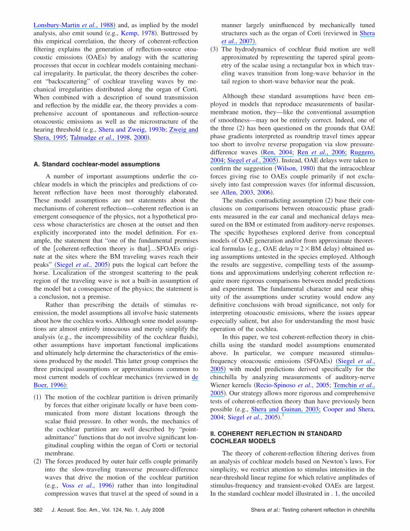
In the standard cochlear model illustrated in . 1, the uncoiledShera et al.: Testing coherent reflection in chinchilla
cochlea appears as a rectangular box filled with incompress-ible, inviscid fluid and subdivided by a flexible membranerepresenting the cochlear partition. Linearized equations offluid dynamics describe the motion of the fluid and its inter-action with the membrane and the boundaries of the box,including the stapes and round window. We describe the me-chanics of the partition by an equivalent point admittancethat characterizes the transverse motion of the organ of Cortiinduced by a pressure difference across its surface. The ad-mittance includes contributions from the active forces in-volved in cochlear amplification. Irregularities are repre-sented as perturbations in the mechanics of the partition.
A. Predicting stimulus-frequency emissions
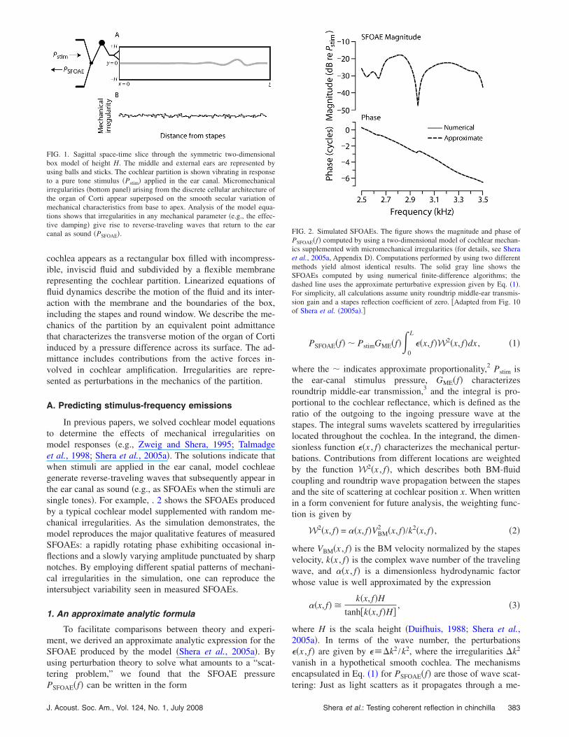
In previous papers, we solved cochlear model equationsto determine the effects of mechanical irregularities onmodel responses �e.g., Zweig and Shera, 1995; Talmadgeet al., 1998; Shera et al., 2005a�. The solutions indicate thatwhen stimuli are applied in the ear canal, model cochleaegenerate reverse-traveling waves that subsequently appear inthe ear canal as sound �e.g., as SFOAEs when the stimuli aresingle tones�. For example, . 2 shows the SFOAEs producedby a typical cochlear model supplemented with random me-chanical irregularities. As the simulation demonstrates, themodel reproduces the major qualitative features of measuredSFOAEs: a rapidly rotating phase exhibiting occasional in-flections and a slowly varying amplitude punctuated by sharpnotches. By employing different spatial patterns of mechani-cal irregularities in the simulation, one can reproduce theintersubject variability seen in measured SFOAEs.
1. An approximate analytic formula
To facilitate comparisons between theory and experi-ment, we derived an approximate analytic expression for theSFOAE produced by the model �Shera et al., 2005a�. Byusing perturbation theory to solve what amounts to a “scat-tering problem,” we found that the SFOAE pressure
FIG. 1. Sagittal space-time slice through the symmetric two-dimensionalbox model of height H. The middle and external ears are represented byusing balls and sticks. The cochlear partition is shown vibrating in responseto a pure tone stimulus �Pstim� applied in the ear canal. Micromechanicalirregularities �bottom panel� arising from the discrete cellular architecture ofthe organ of Corti appear superposed on the smooth secular variation ofmechanical characteristics from base to apex. Analysis of the model equa-tions shows that irregularities in any mechanical parameter �e.g., the effec-tive damping� give rise to reverse-traveling waves that return to the earcanal as sound �PSFOAE�.
PSFOAE�f� can be written in the form
J. Acoust. Soc. Am., Vol. 124, No. 1, July 2008
PSFOAE�f� � PstimGME�f��0
L
��x, f�W2�x, f�dx , �1�
where the � indicates approximate proportionality,2 Pstim isthe ear-canal stimulus pressure, GME�f� characterizesroundtrip middle-ear transmission,3 and the integral is pro-portional to the cochlear reflectance, which is defined as theratio of the outgoing to the ingoing pressure wave at thestapes. The integral sums wavelets scattered by irregularitieslocated throughout the cochlea. In the integrand, the dimen-sionless function ��x , f� characterizes the mechanical pertur-bations. Contributions from different locations are weightedby the function W2�x , f�, which describes both BM-fluidcoupling and roundtrip wave propagation between the stapesand the site of scattering at cochlear position x. When writtenin a form convenient for future analysis, the weighting func-tion is given by
W2�x, f� = ��x, f�VBM2 �x, f�/k2�x, f� , �2�
where VBM�x , f� is the BM velocity normalized by the stapesvelocity, k�x , f� is the complex wave number of the travelingwave, and ��x , f� is a dimensionless hydrodynamic factorwhose value is well approximated by the expression
��x, f� �k�x, f�H
tanh�k�x, f�H�, �3�
where H is the scala height �Duifhuis, 1988; Shera et al.,2005a�. In terms of the wave number, the perturbations��x , f� are given by ���k2 /k2, where the irregularities �k2
vanish in a hypothetical smooth cochlea. The mechanismsencapsulated in Eq. �1� for PSFOAE�f� are those of wave scat-
FIG. 2. Simulated SFOAEs. The figure shows the magnitude and phase ofPSFOAE�f� computed by using a two-dimensional model of cochlear mechan-ics supplemented with micromechanical irregularities �for details, see Sheraet al., 2005a, Appendix D�. Computations performed by using two differentmethods yield almost identical results. The solid gray line shows theSFOAEs computed by using numerical finite-difference algorithms; thedashed line uses the approximate perturbative expression given by Eq. �1�.For simplicity, all calculations assume unity roundtrip middle-ear transmis-sion gain and a stapes reflection coefficient of zero. �Adapted from Fig. 10of Shera et al. �2005a�.�
tering: Just as light scatters as it propagates through a me-
Shera et al.: Testing coherent reflection in chinchilla 383

dium of variable refractive index, so cochlear travelingwaves partially reflect when they encounter irregularities inthe partition mechanics.
Figure 2 establishes the validity of our semianalytic for-mula for PSFOAE�f� �Eq. �1�� by comparing it with the “ex-act” numerical result computed by solving Laplace’s equa-tion using finite-difference algorithms �Shera et al., 2005a�;the two solutions are indistinguishable on the scale of thefigure. By providing knowledge of functional dependenciesnot available from numerical simulations, the semianalyticapproximation proves crucial for subsequent comparisonsbetween theory and experiment.
III. TAILORING PREDICTIONS TO CHINCHILLA
To compare model predictions with SFOAEs measuredin chinchilla �e.g., Siegel et al., 2005�, we need to evaluateEq. �1� for PSFOAE�f� using parameters appropriate to thespecies. The most important quantities to be determined arethose defining the weighting function W2�x , f� given by Eq.�2�. In particular, we need to know the BM velocity responseVBM�x , f� and the complex wave number k�x , f�. The scalaeheight appearing in approximation �3� for ��x , f� can be ob-tained from anatomical measurements �Salt, 2001�.
A. Estimating the traveling wave
By applying Wiener-kernel analysis to auditory-nerve fi-ber �ANF� responses to noise, Ruggero et al. were able toobtain estimates of BM mechanical transfer functions, bothmagnitude and phase, at characteristic frequencies �CFs�throughout the chinchilla cochlea �Recio-Spinoso et al.,2005; Temchin et al., 2005�. As an example, the thin blackline in Fig. 3�A� shows the function VBM�xo , f� obtained froma fiber innervating the base �CF�xo��9 kHz�. The transferfunction is plotted as a function of the “scaling variable,”��x , f�, defined by �Shera, 2007�
��x, f� �f + CF1
CF�x� + CF1, �4�
where the constant CF1 represents the approximate charac-teristic frequency at which the cochlear map morphs fromexponential to more linear behavior in the apex. In the chin-chilla, CF1�140 Hz �Eldredge et al., 1981; Greenwood,1990�. At fixed position, the scaling variable ��x , f� repre-sents a modified normalized frequency that reduces to theconventional form f /CF�x� at frequencies roughly two ormore octaves above CF1. At fixed frequency, equal intervalsof ln � represent constant distances along the BM.
By regarding VBM�x , f� primarily as a function of thesingle variable ��x , f� rather than of the two variables x andf independently, we formalize the local scaling symmetry�Zweig, 1976� manifest by basilar-membrane transfer func-tions �Rhode, 1971; Gummer et al., 1987� and neural tuningcurves �e.g., Kiang and Moxon, 1974; Liberman, 1978�. Asillustrated by the snapshot of the traveling wave shown inFig. 3�B�, local scaling allows one to reinterpret the fre-quency response VBM�xo , f� measured at location xo as anestimate of the spatial response �traveling wave� VBM�x , fo�
at frequency fo; both are given by the function VBM���. The384 J. Acoust. Soc. Am., Vol. 124, No. 1, July 2008
local scaling approximation is most accurate in the regionabout the peak of the response �i.e., for x near xo and for fnear CF�xo��. By converting transfer functions to travelingwaves, local scaling permits computation of the spatial inte-gral appearing in Eq. �1� for PSFOAE�f�.
B. Finding the complex wave number
We obtained the complex wave number of the travelingwave from the Wiener-kernel estimates of VBM�x , f� by usingthe wave number inversion formula derived previously�Shera et al., 2005a; Shera, 2007�,
k2�x, f� = − VBM�x, f��x
L
dx��x�
L
VBM�x�, f�dx�. �5�
The real and imaginary parts of k, known as propagation andgain functions, are denoted as � and �, respectively. Figure3�C� shows the values of ���� and ���� derived from theexample Wiener-kernel estimate of VBM��� shown in panel�A�. The spatial integrals were performed by using local scal-ing.
The properties of the propagation and gain functions ob-tained from the chinchilla Wiener kernels are described andinterpreted elsewhere �Shera, 2007�. Here, we illustrate ourprocedure for validating the inversion procedure by using thederived wave number to reconstruct the BM velocity re-sponse. The thick gray line in Fig. 3�A� shows the functionVBM��� obtained from the wave number in panel �C� by us-ing the Wentzel–Kramers–Brillouin �WKB� formula �Shera
4
FIG. 3. Empirical estimation, inversion, and reconstruction of the BM ve-locity response in chinchilla. Panel �A�: Thin black lines show the magni-tude and phase of the ANF Wiener-kernel estimate of VBM�xo , f� at thecochlear location xo tuned to approximately 9 kHz �Recio-Spinoso et al.,2005�. The scaling variable ��x , f� increases along the logarithmic abscissa.Thick gray lines show the function VBM reconstructed from the derivedwave number �see panel �C�, with k=�+ i�� using the WKB approximation�for details, see Shera, 2007�. Panel �B�: Snapshot of the 9 kHz wave whoseenvelope and phase are shown in panel �A�. The traveling wave was ob-tained by reinterpreting the abscissa as a spatial axis at fixed frequency. Thescale bar represents a distance of 1 mm �Eldredge et al., 1981; Greenwood,1990�. Panel �C�: Solid and dashed lines show propagation and gain func-tions �� and �, respectively� obtained from VBM in panel �A� using the wavenumber inversion formula �Eq. �5��. For reference, thin dashes mark the zeroline. �Adapted from Figs. 2, 4, and 5 of Shera �2007�.�
et al., 2005a�. The agreement with the original measure-
Shera et al.: Testing coherent reflection in chinchilla
ments �thin black line� confirms that the propagation andgain functions obtained from Eq. �5� provide a valid repre-sentation of the complex wave number of the traveling wave.
As detailed elsewhere �Shera, 2007�, we applied the in-version and reconstruction procedure outlined above to eachof the 137 near-threshold Wiener-kernel BM click responsesused to assemble the recently published map of near-CF BMgroup delays �see Fig. 13 of Temchin et al., 2005�. Success-ful reconstructions were obtained for more than 60% of theresponses, representing CFs throughout the cochlea.5 We re-strict further attention to results derived by using these vali-dated responses.
C. Modeling the perturbations
Evaluating the scattering integral in Eq. �1� forPSFOAE�f� requires knowledge of the form and spatial distri-bution of any micromechanical irregularities. Although esti-mates of the weighting function W2�x , f� and wave numberk�x , f� can be obtained for particular cochleae �e.g., by usingthe Wiener kernels�, we have, as yet, no independent meansof estimating the corresponding perturbations, ��x , f���k2 /k2�2�k /k. Although spatial irregularity presumablyoccurs in all mechanical parameters, it seems physiologicallynatural to associate the dominant contribution with irregular-ity in the active forces responsible for traveling-wave ampli-fication. We therefore take �k=r�x���x , f�, where the“roughness” r�x� characterizes the spatial pattern of irregu-larity and ��x , f� is the traveling-wave gain function �Shera,2007�, whose value can be obtained from the wave number��� Im k�. In the short-wave region near the wave peak,irregularities in the gain function � are equivalent to irregu-larities in the real part of the BM admittance.
Since the roughness r�x� remains unknown, we make noattempt to predict SFOAEs in individual ears. Instead, wecompute their statistical behavior �in particular, the distribu-tion of SFOAE phase-gradient delays6� across an ensembleof hypothetical ears, each having the same W2 �i.e., the sameBM velocity response and wave number� but different real-izations of the roughness r�x�. Lacking evidence for moreordered behavior, we also assume that r�x� varies randomlywith position within an ear, displaying the same statisticalfeatures at all locations. The roughness used in the calcula-tions therefore manifests no long-range correlations. Indeed,we assume that the gain function changes randomly and dis-continuously from hair cell to hair cell. However, we obtainequivalent results with much smoother patterns so long asthe roughness r�x� contains spatial frequencies within thepassband of the “spatial-frequency filter” that arises throughthe dynamical action of the traveling wave �see Zweig andShera, 1995, Figs. 6 and 10�.
D. Accounting for middle-ear transmission
For our purposes here, the factor GME�f� describingmiddle-ear transmission can safely be ignored. Although theroundtrip pressure gain �GME� helps determine absoluteemission levels, we cannot confidently predict SFOAE mag-nitudes for other reasons �e.g., we do not know the size of
the irregularities, and the ANF Wiener kernels provide only aJ. Acoust. Soc. Am., Vol. 124, No. 1, July 2008
relative measure of tuning�. Although the middle ear intro-duces a delay �characterized by the phase of GME�, middle-ear delay appears negligible compared to cochlear delay inchinchilla �Ruggero et al., 1990; Songer and Rosowski,2007� and, in any case, is already accounted for by theWiener-kernel transfer functions,7 which were referenced topressure at the eardrum �Recio-Spinoso et al., 2005�.
IV. COMPARING MEASURED AND PREDICTEDSFOAEs
A. Qualitative comparison of SFOAE magnitudeand phase
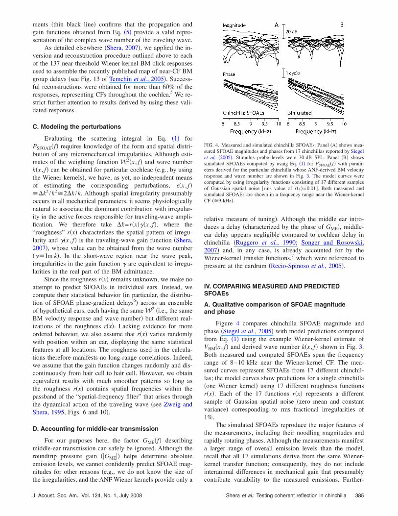
Figure 4 compares chinchilla SFOAE magnitude andphase �Siegel et al., 2005� with model predictions computedfrom Eq. �1� using the example Wiener-kernel estimate ofVBM�x , f� and derived wave number k�x , f� shown in Fig. 3.Both measured and computed SFOAEs span the frequencyrange of 8–10 kHz near the Wiener-kernel CF. The mea-sured curves represent SFOAEs from 17 different chinchil-las; the model curves show predictions for a single chinchilla�one Wiener kernel� using 17 different roughness functionsr�x�. Each of the 17 functions r�x� represents a differentsample of Gaussian spatial noise �zero mean and constantvariance� corresponding to rms fractional irregularities of1%.
The simulated SFOAEs reproduce the major features ofthe measurements, including their noodling magnitudes andrapidly rotating phases. Although the measurements manifesta larger range of overall emission levels than the model,recall that all 17 simulations derive from the same Wiener-kernel transfer function; consequently, they do not includeinteranimal differences in mechanical gain that presumably
FIG. 4. Measured and simulated chinchilla SFOAEs. Panel �A� shows mea-sured SFOAE magnitudes and phases from 17 chinchillas reported by Siegelet al. �2005�. Stimulus probe levels were 30 dB SPL. Panel �B� showssimulated SFOAEs computed by using Eq. �1� for PSFOAE�f� with param-eters derived for the particular chinchilla whose ANF-derived BM velocityresponse and wave number are shown in Fig. 3. The model curves werecomputed by using irregularity functions consisting of 17 different samplesof Gaussian spatial noise �rms value of r�x�=0.01�. Both measured andsimulated SFOAEs are shown in a frequency range near the Wiener-kernelCF ��9 kHz�.
contribute variability to the measured emissions. Further-
Shera et al.: Testing coherent reflection in chinchilla 385
more, because the model roughness functions are all drawnfrom the same Gaussian distribution, their statistical features�e.g., rms value� are almost certainly more uniform thanthose of their biological counterparts. As for the phase, mea-sured and predicted phase-gradient delays are similar; themean delay obtained using the example Wiener kernel fromFig. 3 �1.4 ms� falls within the interquartile range of the 17measurements. Undulations in emission magnitude �e.g., theoccasional deep notches� correlate with wobbles in thephase, as expected from constraints imposed by causality�Sisto et al., 2007�.
Because intra- and interanimal variations in middle-eartransmission and cochlear gain have considerable effects onOAE amplitude but are difficult to control for using thesedata, we focus our attention here on comparisons involvingemission phase, specifically the SFOAE phase-gradient de-lay.
B. Preliminary comparison of delays throughoutthe cochlea
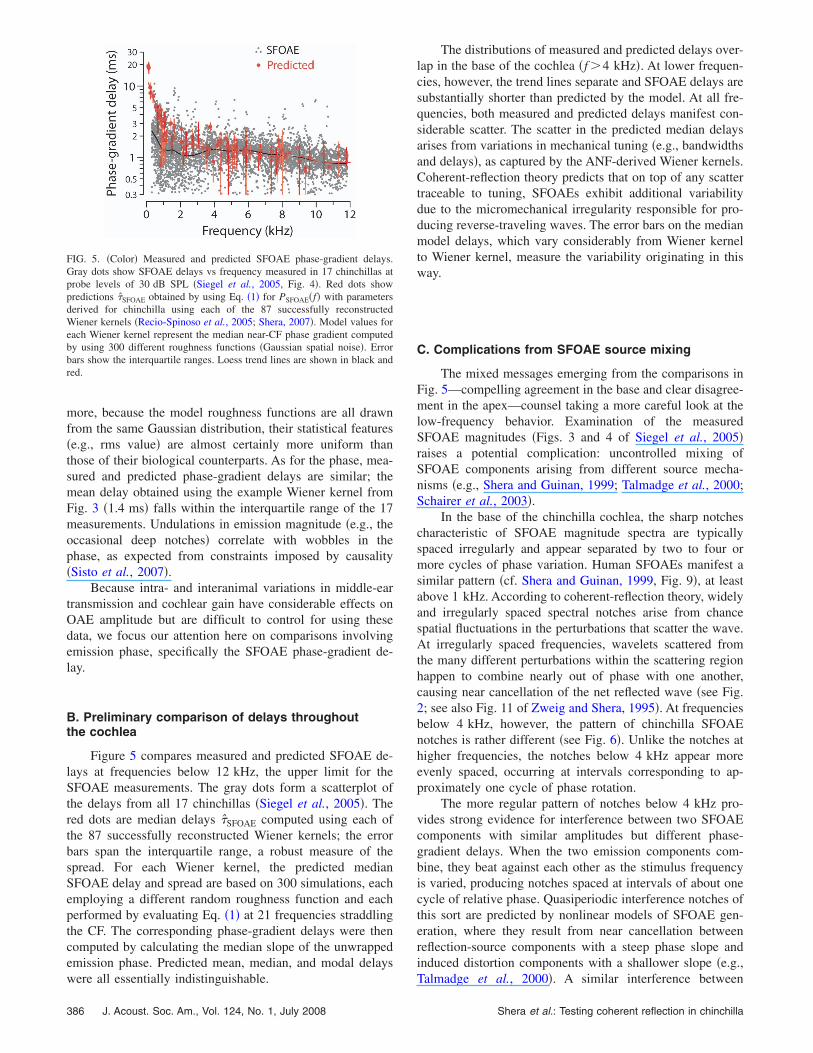
Figure 5 compares measured and predicted SFOAE de-lays at frequencies below 12 kHz, the upper limit for theSFOAE measurements. The gray dots form a scatterplot ofthe delays from all 17 chinchillas �Siegel et al., 2005�. Thered dots are median delays �̂SFOAE computed using each ofthe 87 successfully reconstructed Wiener kernels; the errorbars span the interquartile range, a robust measure of thespread. For each Wiener kernel, the predicted medianSFOAE delay and spread are based on 300 simulations, eachemploying a different random roughness function and eachperformed by evaluating Eq. �1� at 21 frequencies straddlingthe CF. The corresponding phase-gradient delays were thencomputed by calculating the median slope of the unwrappedemission phase. Predicted mean, median, and modal delays
FIG. 5. �Color� Measured and predicted SFOAE phase-gradient delays.Gray dots show SFOAE delays vs frequency measured in 17 chinchillas atprobe levels of 30 dB SPL �Siegel et al., 2005, Fig. 4�. Red dots showpredictions �̂SFOAE obtained by using Eq. �1� for PSFOAE�f� with parametersderived for chinchilla using each of the 87 successfully reconstructedWiener kernels �Recio-Spinoso et al., 2005; Shera, 2007�. Model values foreach Wiener kernel represent the median near-CF phase gradient computedby using 300 different roughness functions �Gaussian spatial noise�. Errorbars show the interquartile ranges. Loess trend lines are shown in black andred.
were all essentially indistinguishable.
386 J. Acoust. Soc. Am., Vol. 124, No. 1, July 2008
The distributions of measured and predicted delays over-lap in the base of the cochlea �f 4 kHz�. At lower frequen-cies, however, the trend lines separate and SFOAE delays aresubstantially shorter than predicted by the model. At all fre-quencies, both measured and predicted delays manifest con-siderable scatter. The scatter in the predicted median delaysarises from variations in mechanical tuning �e.g., bandwidthsand delays�, as captured by the ANF-derived Wiener kernels.Coherent-reflection theory predicts that on top of any scattertraceable to tuning, SFOAEs exhibit additional variabilitydue to the micromechanical irregularity responsible for pro-ducing reverse-traveling waves. The error bars on the medianmodel delays, which vary considerably from Wiener kernelto Wiener kernel, measure the variability originating in thisway.
C. Complications from SFOAE source mixing
The mixed messages emerging from the comparisons inFig. 5—compelling agreement in the base and clear disagree-ment in the apex—counsel taking a more careful look at thelow-frequency behavior. Examination of the measuredSFOAE magnitudes �Figs. 3 and 4 of Siegel et al., 2005�raises a potential complication: uncontrolled mixing ofSFOAE components arising from different source mecha-nisms �e.g., Shera and Guinan, 1999; Talmadge et al., 2000;Schairer et al., 2003�.
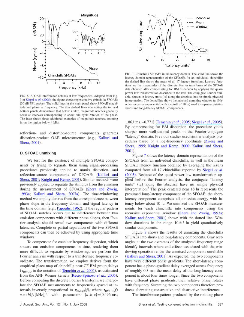
In the base of the chinchilla cochlea, the sharp notchescharacteristic of SFOAE magnitude spectra are typicallyspaced irregularly and appear separated by two to four ormore cycles of phase variation. Human SFOAEs manifest asimilar pattern �cf. Shera and Guinan, 1999, Fig. 9�, at leastabove 1 kHz. According to coherent-reflection theory, widelyand irregularly spaced spectral notches arise from chancespatial fluctuations in the perturbations that scatter the wave.At irregularly spaced frequencies, wavelets scattered fromthe many different perturbations within the scattering regionhappen to combine nearly out of phase with one another,causing near cancellation of the net reflected wave �see Fig.2; see also Fig. 11 of Zweig and Shera, 1995�. At frequenciesbelow 4 kHz, however, the pattern of chinchilla SFOAEnotches is rather different �see Fig. 6�. Unlike the notches athigher frequencies, the notches below 4 kHz appear moreevenly spaced, occurring at intervals corresponding to ap-proximately one cycle of phase rotation.
The more regular pattern of notches below 4 kHz pro-vides strong evidence for interference between two SFOAEcomponents with similar amplitudes but different phase-gradient delays. When the two emission components com-bine, they beat against each other as the stimulus frequencyis varied, producing notches spaced at intervals of about onecycle of relative phase. Quasiperiodic interference notches ofthis sort are predicted by nonlinear models of SFOAE gen-eration, where they result from near cancellation betweenreflection-source components with a steep phase slope andinduced distortion components with a shallower slope �e.g.,
Talmadge et al., 2000�. A similar interference betweenShera et al.: Testing coherent reflection in chinchilla
reflection- and distortion-source components generatesdistortion-product OAE microstructure �e.g., Kalluri andShera, 2001�.
D. SFOAE unmixing
We test for the existence of multiple SFOAE compo-nents by trying to separate them using signal-processingprocedures previously applied to unmix distortion- andreflection-source components of DPOAEs �Kalluri andShera, 2001; Knight and Kemp, 2001�. Similar methods werepreviously applied to separate the stimulus from the emissionduring the measurement of SFOAEs �Shera and Zweig,1993a; Kalluri and Shera, 2007a�. The time-windowingmethod we employ derives from the correspondence betweenphase slope in the frequency domain and signal latency inthe time domain �e.g., Papoulis, 1962�. If the regular patternof SFOAE notches occurs due to interference between twoemission components with different phase slopes, then Fou-rier analysis should reveal two components with differentlatencies. Complete or partial separation of the two SFOAEcomponents can then be achieved by using appropriate timewindows.
To compensate for cochlear frequency dispersion, whichsmears out emission components in time, rendering themmore difficult to separate by windowing, we perform theFourier analysis with respect to a transformed frequency co-ordinate. The transformation we employ derives from theempirical place map of chinchilla near-CF BM group delays��BMGD in the notation of Temchin et al. 2005�, as estimatedfrom the ANF Wiener kernels �Recio-Spinoso et al., 2005�.Before computing the discrete Fourier transform, we interpo-late the SFOAE measurements to frequencies spaced at in-tervals inversely proportional to �BMGD�f�, where �BMGD�f�
c
FIG. 6. SFOAE interference notches at low frequencies. Adapted from Fig.3 of Siegel et al. �2005�, the figure shows representative chinchilla SFOAEs�30 dB SPL probe�. The solid lines in the main panel show SFOAE magni-tude and phase vs frequency. The thin dashed lines connecting the top andbottom panels demonstrate that below 4 kHz, magnitude notches generallyoccur at intervals corresponding to about one cycle rotation of the phase.The inset shows three additional examples of magnitude notches, zoomingin on the region below 4 kHz.
=a+b�f / �kHz�� with parameters �a ,b ,c�= �0.496 ms,
J. Acoust. Soc. Am., Vol. 124, No. 1, July 2008
1.863 ms,−0.771� �Temchin et al., 2005; Siegel et al., 2005�.By compensating for BM dispersion, the procedure yieldssharper more well-defined peaks in the Fourier-conjugate“latency” domain. Previous studies used similar analysis pro-cedures based on a log-frequency coordinate �Zweig andShera, 1995; Knight and Kemp, 2000; Kalluri and Shera,2001�.
Figure 7 shows the latency-domain representation of theSFOAEs from an individual chinchilla, as well as the meanSFOAE latency function obtained by averaging the resultscomputed from all 17 chinchillas reported by Siegel et al.�2005�. Because of the quasi-power-law transformation ap-plied before the Fourier analysis, the conjugate “latencyunits” �lu� along the abscissa have no simple physicalinterpretation.8 The peak centered near 18 lu represents thepresumed long-latency component of the SFOAE; the short-latency component comprises all emission energy with la-tency below about 10 lu. We unmixed the SFOAE measure-ments for each chinchilla into components using therecursive exponential window �Shera and Zweig, 1993a;Kalluri and Shera, 2001� shown with the dotted line. Win-dow durations in the range 103 lu yield quantitativelysimilar components.
Figure 8 shows the results of unmixing the chinchillaSFOAEs into short- and long-latency components. Gray rect-angles at the two extremes of the analyzed frequency rangeidentify intervals where end effects associated with the win-dowing operation render the unmixed components unreliable�Kalluri and Shera, 2001�. As expected, the two componentshave very different phase gradients. The short-latency com-ponent has a phase-gradient delay averaged across frequencyof roughly 0.3 ms; the mean delay of the long-latency com-ponent is about four times longer. Since the two componentshave different phase gradients, their relative phase rotateswith frequency. Summing the two components therefore pro-duces alternating constructive and destructive interference.
FIG. 7. Chinchilla SFOAEs in the latency domain. The solid line shows thelatency-domain representation of the SFOAEs for an individual chinchilla;the dashed line shows the mean of all 17 latency functions. Latency func-tions are the magnitudes of the discrete Fourier transforms of the SFOAEdata obtained after compensating for BM dispersion by applying the quasi-power-law transformation described in the text. The conjugate Fourier vari-able, shown in latency units �lu� along the abscissa, has no simple physicalinterpretation. The dotted line shows the matched unmixing window �a 10th-order recursive exponential with a cutoff of 10 lu� used to separate putativeshort- and long-latency SFOAE components.
The interference pattern produced by the rotating phase
Shera et al.: Testing coherent reflection in chinchilla 387
depends on the component magnitudes. Figure 8 shows thatthe relative magnitude of the two components undergoes anabrupt transition near 4 kHz. At frequencies above 4 kHz,the long-latency component dominates the total emission,and the median level difference between the components ex-ceeds 10 dB. Below 4 kHz, however, the median levels ofthe two components are nearly equal; on average, the short-latency component is about 1 dB larger than the long-latencycomponent. In the low-frequency region, the similarity incomponent magnitudes, combined with the rotation of theirrelative phase, produces near cancellation at regular inter-vals. The two unmixed components therefore have propertiesconsistent with the quasiperiodic interference notches ob-served below 4 kHz �and with their absence at higher fre-quencies�. Although definitive conclusions require indepen-dent evidence for multiple SFOAE components, theunmixing analysis strongly suggests that chinchilla SFOAEsare indeed mixtures produced by multiple mechanisms, atleast below 4 kHz.
E. Comparison of unmixed delays
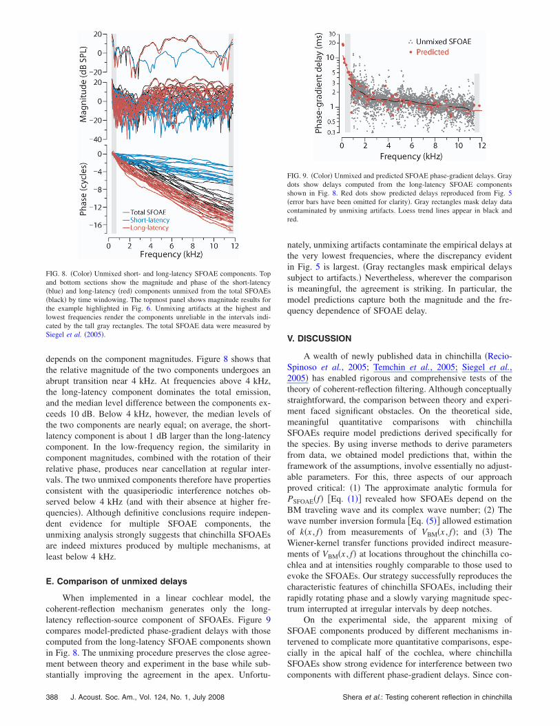
When implemented in a linear cochlear model, thecoherent-reflection mechanism generates only the long-latency reflection-source component of SFOAEs. Figure 9compares model-predicted phase-gradient delays with thosecomputed from the long-latency SFOAE components shownin Fig. 8. The unmixing procedure preserves the close agree-ment between theory and experiment in the base while sub-
FIG. 8. �Color� Unmixed short- and long-latency SFOAE components. Topand bottom sections show the magnitude and phase of the short-latency�blue� and long-latency �red� components unmixed from the total SFOAEs�black� by time windowing. The topmost panel shows magnitude results forthe example highlighted in Fig. 6. Unmixing artifacts at the highest andlowest frequencies render the components unreliable in the intervals indi-cated by the tall gray rectangles. The total SFOAE data were measured bySiegel et al. �2005�.
stantially improving the agreement in the apex. Unfortu-
388 J. Acoust. Soc. Am., Vol. 124, No. 1, July 2008
nately, unmixing artifacts contaminate the empirical delays atthe very lowest frequencies, where the discrepancy evidentin Fig. 5 is largest. �Gray rectangles mask empirical delayssubject to artifacts.� Nevertheless, wherever the comparisonis meaningful, the agreement is striking. In particular, themodel predictions capture both the magnitude and the fre-quency dependence of SFOAE delay.
V. DISCUSSION
A wealth of newly published data in chinchilla �Recio-Spinoso et al., 2005; Temchin et al., 2005; Siegel et al.,2005� has enabled rigorous and comprehensive tests of thetheory of coherent-reflection filtering. Although conceptuallystraightforward, the comparison between theory and experi-ment faced significant obstacles. On the theoretical side,meaningful quantitative comparisons with chinchillaSFOAEs require model predictions derived specifically forthe species. By using inverse methods to derive parametersfrom data, we obtained model predictions that, within theframework of the assumptions, involve essentially no adjust-able parameters. For this, three aspects of our approachproved critical: �1� The approximate analytic formula forPSFOAE�f� �Eq. �1�� revealed how SFOAEs depend on theBM traveling wave and its complex wave number; �2� Thewave number inversion formula �Eq. �5�� allowed estimationof k�x , f� from measurements of VBM�x , f�; and �3� TheWiener-kernel transfer functions provided indirect measure-ments of VBM�x , f� at locations throughout the chinchilla co-chlea and at intensities roughly comparable to those used toevoke the SFOAEs. Our strategy successfully reproduces thecharacteristic features of chinchilla SFOAEs, including theirrapidly rotating phase and a slowly varying magnitude spec-trum interrupted at irregular intervals by deep notches.
On the experimental side, the apparent mixing ofSFOAE components produced by different mechanisms in-tervened to complicate more quantitative comparisons, espe-cially in the apical half of the cochlea, where chinchillaSFOAEs show strong evidence for interference between two
FIG. 9. �Color� Unmixed and predicted SFOAE phase-gradient delays. Graydots show delays computed from the long-latency SFOAE componentsshown in Fig. 8. Red dots show predicted delays reproduced from Fig. 5�error bars have been omitted for clarity�. Gray rectangles mask delay datacontaminated by unmixing artifacts. Loess trend lines appear in black andred.
components with different phase-gradient delays. Since con-
Shera et al.: Testing coherent reflection in chinchilla
tamination by multiple OAE components confounds straight-forward comparisons between theory and experiment, weused signal-processing techniques to “unmix” the measuredSFOAEs. Although definitive characterization of SFOAEcomponents requires independent corroboration, the unmix-ing analysis revealed emission components with the proper-ties necessary to reproduce the interference pattern evident inthe total SFOAE. As a result, we were able to comparemodel predictions with both the total SFOAEs and with theirputative reflection-source components. Model comparisonswith the total SFOAEs yield strong agreement in the base butsubstantial discrepancies below 4 kHz, where the relativemagnitude of the short-latency component is greatest. Un-mixing the SFOAEs preserves the model’s success in thebase while significantly improving the agreement in theapex.
A. Relationship between SFOAE and BM delay
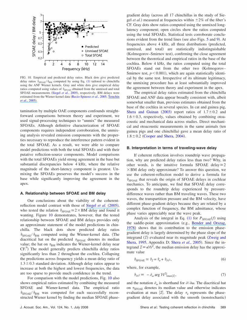
Our conclusions about the viability of the coherent-reflection model contrast with those of Siegel et al. �2005�,who tested the relation �̂SFOAE�2�BM delay and found itwanting. Figure 10 demonstrates, however, that the testedrelationship between SFOAE and BM delays provides onlyan approximate statement of the model predictions in chin-chilla. The black dots show predicted delay ratios�̂SFOAE / �̂BM computed using the Wiener-kernel data. �Thediacritical hat on the predicted �SFOAE denotes its medianvalue; the hat on �BM indicates the Wiener-kernel delay nearCF.9� The model generally predicts chinchilla delay ratiossignificantly less than 2 throughout the cochlea. Collapsingthe predictions across frequency yields a mean delay ratio of1.30.3 standard deviation. Although delay ratios appear toincrease at both the highest and lowest frequencies, the dataare too sparse to provide much confidence in the trend.
For comparison with the model predictions, Fig. 10 alsoshows empirical ratios estimated by combining the measuredSFOAE and Wiener-kernel data. The empirical ratio�̂SFOAE / �̂BM was computed for each successfully recon-
FIG. 10. Empirical and predicted delay ratios. Black dots give predicteddelay ratios �̂SFOAE / �̂BM computed by using Eq. �1� tailored to chinchillausing the ANF Wiener kernels. Gray and white dots give empirical delayratios computed using values of �̂SFOAE obtained from the unmixed and totalSFOAE measurements �Siegel et al., 2005�, respectively. BM delays wereestimated from the Wiener-kernel data �Recio-Spinoso et al., 2005; Temchinet al., 2005�.
structed Wiener kernel by finding the median SFOAE phase-
J. Acoust. Soc. Am., Vol. 124, No. 1, July 2008
gradient delay �across all 17 chinchillas in the study of Sie-gel et al.� measured at frequencies within 2% of the fiber’sCF. Gray dots show ratios computed using the unmixed long-latency component; open circles show the ratios computedusing the total SFOAEs. Statistical tests corroborate conclu-sions evident from the trend lines �see also Figs. 5 and 9�. Atfrequencies above 4 kHz, all three distributions �predicted,unmixed, and total� are statistically indistinguishable�Kolmogorov–Smirnov test�, confirming the close agreementbetween the theoretical and empirical ratios in the base of thecochlea. Below 4 kHz, the ratios computed using the totalSFOAEs stand out from the other two �Kolmogorov–Smirnov test, p�0.001�, which are again statistically identi-cal by the same test. Irrespective of its ultimate legitimacy,the unmixing procedure has at least substantially improvedthe agreement between theory and experiment in the apex.
The empirical delay ratios estimated from the chinchillaSFOAE and ANF data appear broadly consistent with, albeitsomewhat smaller than, previous estimates obtained from thebase of the cochlea in several species. In cat and guinea pig,Shera and Guinan �2003� report ratios of 1.70.2 and1.60.3, respectively, values obtained by combining otoa-coustic and mechanical data across studies. Direct mechani-cal and otoacoustic measurements in the same animals �tenguinea pigs and one chinchilla� gave a mean delay ratio of1.80.2 �Cooper and Shera, 2004�.
B. Interpretation in terms of traveling-wave delay
If coherent reflection involves roundtrip wave propaga-tion, why are predicted delay ratios less than two? Why, inother words, is the intuitive formula SFOAE delay�2�BM delay only approximate? To answer this question, weuse the coherent-reflection model to derive a formula for�̂SFOAE that reveals the origin of SFOAE delays in cochlearmechanics. To anticipate, we find that SFOAE delay corre-sponds to the roundtrip delay experienced by pressure-difference waves rather than BM traveling waves. These twowaves, the transpartition pressure and the BM velocity, havedifferent phase-gradient delays because they are related by acomplex function of frequency, the BM admittance, whosephase varies appreciably near the wave peak.
Analysis of the integral in Eq. �1� for PSFOAE�f� usingthe saddle-point approximation �e.g., Bender and Orszag,1978� shows that its contribution to the emission phase-gradient delay is largely determined by the phase slope of theintegrand �I� evaluated near its magnitude peak �Zweig andShera, 1995, Appendix D; Shera et al., 2005�. Since the in-tegrand I��W2, the median emission delay has the approxi-mate value
�̂SFOAE � �̂I = �̂� + �̂W2, �6�
where, for example,
�̂W2 � − �� arg W2maxI, �7�
and the notation �� is shorthand for � /��. The diacritical haton �SFOAE denotes its median value and otherwise indicatesevaluation at max I. The delay �� represents the phase-
gradient delay associated with the smooth �nonstochastic�Shera et al.: Testing coherent reflection in chinchilla 389
component of the perturbations. Equation �6� accurately pre-dicts �̂SFOAE in both one- and two-dimensional active co-chlear models �cf. Fig. 12 of Shera et al., 2005a�.
Approximation �6� for �̂SFOAE can be expressed by usingquantities determined by the Wiener-kernel measurements.We begin by examining the forms of � and W2 appearing inthe integrand. Recall that we took ��x , f��2�k /k with �k=r�x���x , f�, where ��x , f� is the gain function. Because �kis real, it makes no contribution to the phase of �. Hence,���−�k, where �̂k is the phase-gradient delay of the wavenumber ��k�−�� arg k�; �k enters with a minus sign becausek resides in the denominator �arg k−1=−arg k�. Equation �2�for W2 simplifies in the short-wave regime near the wavepeak. In the short-wave limit, �→kH so that W2
��VBM2 /k2�HVBM
2 /k. Hence �̂W2 �2�̂BM− �̂k, where thefactor of 2 comes from the exponent on VBM, and �k againenters with a minus sign.
Combining the expressions for �̂� and �̂W2 yields theapproximation
�̂SFOAE � 2��̂BM − �̂k� . �8�
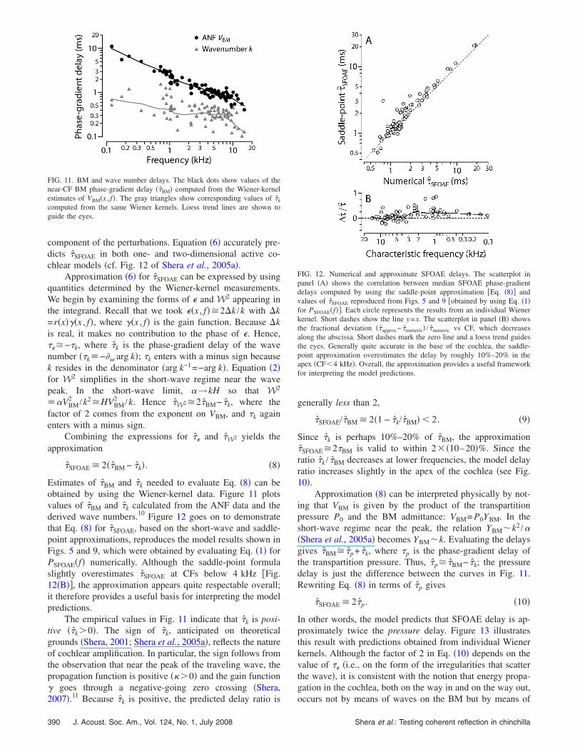
Estimates of �̂BM and �̂k needed to evaluate Eq. �8� can beobtained by using the Wiener-kernel data. Figure 11 plotsvalues of �̂BM and �̂k calculated from the ANF data and thederived wave numbers.10 Figure 12 goes on to demonstratethat Eq. �8� for �̂SFOAE, based on the short-wave and saddle-point approximations, reproduces the model results shown inFigs. 5 and 9, which were obtained by evaluating Eq. �1� forPSFOAE�f� numerically. Although the saddle-point formulaslightly overestimates �̂SFOAE at CFs below 4 kHz �Fig.12�B��, the approximation appears quite respectable overall;it therefore provides a useful basis for interpreting the modelpredictions.
The empirical values in Fig. 11 indicate that �̂k is posi-tive ��̂k0�. The sign of �̂k, anticipated on theoreticalgrounds �Shera, 2001; Shera et al., 2005a�, reflects the natureof cochlear amplification. In particular, the sign follows fromthe observation that near the peak of the traveling wave, thepropagation function is positive ��0� and the gain function� goes through a negative-going zero crossing �Shera,
11 ˆ
FIG. 11. BM and wave number delays. The black dots show values of thenear-CF BM phase-gradient delay ��̂BM� computed from the Wiener-kernelestimates of VBM�x , f�. The gray triangles show corresponding values of �̂k
computed from the same Wiener kernels. Loess trend lines are shown toguide the eyes.
2007�. Because �k is positive, the predicted delay ratio is
390 J. Acoust. Soc. Am., Vol. 124, No. 1, July 2008
generally less than 2,
�̂SFOAE/�̂BM � 2�1 − �̂k/�̂BM� � 2. �9�
Since �̂k is perhaps 10%–20% of �̂BM, the approximation�̂SFOAE�2�BM is valid to within 2� �10–20�%. Since theratio �̂k / �̂BM decreases at lower frequencies, the model delayratio increases slightly in the apex of the cochlea �see Fig.10�.
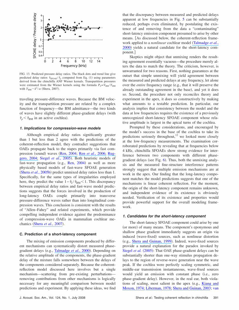
Approximation �8� can be interpreted physically by not-ing that VBM is given by the product of the transpartitionpressure P0 and the BM admittance: VBM= P0YBM. In theshort-wave regime near the peak, the relation YBM�k2 /��Shera et al., 2005a� becomes YBM�k. Evaluating the delaysgives �̂BM� �̂p+ �̂k, where �p is the phase-gradient delay ofthe transpartition pressure. Thus, �̂p� �̂BM− �̂k; the pressuredelay is just the difference between the curves in Fig. 11.Rewriting Eq. �8� in terms of �̂p gives
�̂SFOAE � 2�̂p. �10�
In other words, the model predicts that SFOAE delay is ap-proximately twice the pressure delay. Figure 13 illustratesthis result with predictions obtained from individual Wienerkernels. Although the factor of 2 in Eq. �10� depends on thevalue of �� �i.e., on the form of the irregularities that scatterthe wave�, it is consistent with the notion that energy propa-gation in the cochlea, both on the way in and on the way out,
FIG. 12. Numerical and approximate SFOAE delays. The scatterplot inpanel �A� shows the correlation between median SFOAE phase-gradientdelays computed by using the saddle-point approximation �Eq. �8�� andvalues of �̂SFOAE reproduced from Figs. 5 and 9 �obtained by using Eq. �1�for PSFOAE�f��. Each circle represents the results from an individual Wienerkernel. Short dashes show the line y=x. The scatterplot in panel �B� showsthe fractional deviation ��̂approx− �̂numeric� / �̂numeric vs CF, which decreasesalong the abscissa. Short dashes mark the zero line and a loess trend guidesthe eyes. Generally quite accurate in the base of the cochlea, the saddle-point approximation overestimates the delay by roughly 10%–20% in theapex �CF�4 kHz�. Overall, the approximation provides a useful frameworkfor interpreting the model predictions.
occurs not by means of waves on the BM but by means of
Shera et al.: Testing coherent reflection in chinchilla
traveling pressure-difference waves. Because the BM veloc-ity and the transpartition pressure are related by a complexfunction of frequency—the BM admittance—the two kindsof waves have slightly different phase-gradient delays �with�̂p��̂BM in an active cochlea�.
1. Implications for compression-wave models
Although empirical delay ratios significantly greaterthan 1 but less than 2 agree with the predictions of thecoherent-reflection model, they contradict suggestions thatOAEs propagate back to the stapes primarily via fast com-pression �sound� waves �Ren, 2004; Ren et al., 2006; Rug-gero, 2004; Siegel et al., 2005�. Both heuristic models offast-wave propagation �e.g., Ren, 2004� as well as morephysically based models of fast-wave SFOAE generation�Shera et al., 2005b� predict unmixed delay ratios less than 1.Specifically, for the same types of irregularities employedhere, they predict the value 1− �̂k / �̂BM�1. This discrepancybetween empirical delay ratios and fast-wave model predic-tions suggests that the forces involved in the production oflong-latency OAEs couple primarily into transversepressure-difference waves rather than into longitudinal com-pression waves. This conclusion is consistent with the resultsof “Allen–Fahey” and related experiments, which providecompelling independent evidence against the predominanceof compression-wave OAEs in mammalian cochlear me-chanics �Shera et al., 2007�.
C. Prediction of a short-latency component
The mixing of emission components produced by differ-ent mechanisms can systematically distort measured phase-gradient delays �e.g., Talmadge et al., 2000�. Depending onthe relative amplitude of the components, the phase-gradientdelay of the mixture falls somewhere between the delays ofthe components considered separately. Because the coherent-reflection model discussed here involves but a singlemechanism—scattering from pre-existing perturbations—removing contributions from other mechanisms is logicallynecessary for any meaningful comparison between model
FIG. 13. Predicted pressure delay ratios. The black dots and trend line givepredicted delay ratios �̂SFOAE / �̂p computed from Eq. �1� using parametersderived from the chinchilla ANF Wiener kernals. Transpartition pressureswere estimated from the Wiener kernels using the formula P0=VBM /YBM
with YBM�k2 /� �Shera, 2007�.
predictions and experiment. By applying these ideas, we find
J. Acoust. Soc. Am., Vol. 124, No. 1, July 2008
that the discrepancy between measured and predicted delaysapparent at low frequencies in Fig. 5 can be substantiallyreduced, perhaps even eliminated, by postulating the exis-tence of and removing from the data a “contaminating”short-latency emission component presumed to arise by othermeans. �As discussed below, the coherent-reflection frame-work applied to a nonlinear cochlear model �Talmadge et al.,2000� yields a natural candidate for the short-latency com-ponent.�
Skeptics might object that unmixing renders the result-ing agreement essentially vacuous—the procedure merely al-ters the data to match the theory. The criticism, however, isunwarranted for two reasons. First, nothing guarantees at theoutset that simple unmixing will yield agreement betweenthe measured and predicted delays at any frequency, let aloneover the entire frequency range �e.g., that it will preserve thealready outstanding agreement in the base�, and yet it doesso. Second, the procedure not only reconciles theory andexperiment in the apex, it does so constructively by makingwhat amounts to a testable prediction. In particular, ouranalysis implies that consistency between the model and thedata at low frequencies requires the existence of a previouslyunrecognized short-latency SFOAE component whose rela-tive amplitude is largest in the apical turns of the cochlea.
Prompted by these considerations, and encouraged bythe model’s success in the base of the cochlea to take itspredictions seriously throughout,12 we looked more closelyat the low-frequency measurements. The examination cor-roborated predictions by revealing that at frequencies below4 kHz, chinchilla SFOAEs show strong evidence for inter-ference between two components with different phase-gradient delays �see Fig. 6�. Thus, both the unmixing analy-sis and the measured fine-structure interference patternsstrongly suggest that multiple emission mechanisms are atwork in the apex. Our finding that the long-latency compo-nent matches the model predictions suggests that one of themechanisms is linear coherent reflection. For the moment,the origin of the short-latency component remains unknown,and independent evidence of its existence is obviouslyneeded. Verification of its existence and properties wouldprovide powerful support for the overall modeling frame-work.
1. Candidates for the short-latency component
The short-latency SFOAE component could arise by one�or more� of many means. The component’s eponymous andshallow phase gradient immediately suggests an origin viainduced �wave-fixed� sources, such as nonlinear distortion�e.g., Shera and Guinan, 1999�. Indeed, wave-fixed sourcesprovide a natural explanation for the paradox invoked bySiegel et al. �2005�: That OAE phase-gradient delays can besubstantially shorter than one-way stimulus propagation de-lays to the region of reverse-wave generation near the wavepeak. If the cochlea were perfectly scaling symmetric, andmiddle-ear transmission instantaneous, wave-fixed sourceswould yield an emission with constant phase �i.e., zerophase-gradient delay�. However, in the real ear, both viola-tions of scaling, most salient in the apex �e.g., Kiang and
Moxon, 1974; Liberman, 1978; Shera and Guinan, 2003; vanShera et al.: Testing coherent reflection in chinchilla 391
der Heijden and Joris, 2006�, and finite middle-ear delays�e.g., Dong and Olson, 2006� can produce small but nonzerophase-gradient delays at least qualitatively similar to thoseapparent in Fig. 9.
Helpfully, the coherent-reflection framework itself pro-vides what may be the most natural candidate for the short-latency component: wave-fixed emissions that arise by scat-tering off wave-induced perturbations created bynonlinearities in the mechanics �i.e., the process dubbed“nonlinear reflection” �Talmadge et al., 2000��. Although thepresent analysis employed linear cochlear models, the actualcochlea is nonlinear, even at the relatively low levels usedfor the SFOAE measurements. Adding both mechanical ir-regularity and nonlinearity to active models produces a mix-ture of wave- and place-fixed SFOAEs qualitatively similarto that seen here and in other studies �Talmadge et al., 2000;Goodman et al., 2003; Schairer et al., 2003�. In addition,simple compression-wave models predict that OAEs gener-ated by coupling into fast waves �e.g., via volume-velocitysources in the organ of Corti� are also essentially wave fixed�Shera et al., 2005b� and could, in principle, be contributingto the short-latency component.
The short-latency component could also comprise emis-sion components that arise from the tail region of the co-chlear traveling wave rather than the peak. Because thewavelength of the traveling wave is generally longer in thetail region, even place-fixed mechanisms acting in this regioncould produce emissions with relatively shallow phase gra-dients. Although their interpretation is not unequivocal�Shera et al., 2004�, suppression experiments suggest thatcontributions from the tail of the traveling wave may, in fact,be significant in chinchilla �Siegel et al., 2003, 2004�.
Alternatively, the appearance of a significant short-latency SFOAE component in the apex could simply be anartifact of the measurement method, which relies on nonlin-ear interactions between the probe and the suppressor to ex-tract the emission. If the form and/or frequency dependenceof cochlear nonlinearities differ markedly between the baseand the apex �e.g., Khanna and Hao, 1999; Cooper andDong, 2003�, then the suppression method may not alwaysreliably extract the principal emission evoked by the probe�cf. Kalluri and Shera, 2007a�. As an extreme example, sup-pose that the mechanics in the apex were completely linearand exhibited no two-tone suppression. Then, even if theapex were to generate strong reflection-source OAEs, sup-pression and other “nonlinear” methods would be unable tomeasure them. Hence, if low-frequency OAEs were actuallyrecorded by using these methods, then the measured emis-sions could only have originated from more basal �nonlinear�regions of the cochlea �i.e., from regions corresponding tothe tail of the traveling wave�. As a result, the measuredphase-gradient delays would be correspondingly reduced. Inthe actual ear, the suppression method may extract a mix ofemissions from tip and tail regions of the traveling wavewhose relative amplitudes vary with CF, depending on theform of cochlear mechanical nonlinearities.
Finally, and most speculatively, the short-latency com-ponent may arise through the involvement of nontraditional
modes of energy propagation in the cochlea. If the relative392 J. Acoust. Soc. Am., Vol. 124, No. 1, July 2008
magnitude of the short-latency component is any guide, thesemodes presumably play a more important role in the me-chanics of the apex than in the base. Evidence for multiplemodes of motion in this CF region can be found in ANFclick responses �Lin and Guinan, 2004; Guinan et al., 2005�and in tuning curves, which have multilobed tips and groupdelays that change abruptly at the seams �e.g., Pfeiffer andMolnar, 1970; Kiang, 1984; van der Heijden and Joris,2003�.
D. An apical-basal transition
Independent of the status of the coherent-reflectionmodel or of the existence or identity of any short-latencyemission component, our analysis suggests that the chin-chilla cochlea undergoes a transition between more “apical-like” and more “basal-like” behavior near the 4 kHz place. InFig. 10, for example, empirical delay ratios �̂SFOAE / �̂BM com-puted from the total SFOAEs change slope rather abruptlynear 4 kHz; they increase with frequency below 4 kHz butremain almost constant above. The appearance of this mid-frequency transition is due almost entirely to a change in thefrequency dependence of �̂SFOAE rather than of �̂BM. Interest-ingly, a similar midfrequency bend in �̂SFOAE occurs in othermammals, including cats, guinea pigs, and humans �Sheraand Guinan, 2003�. In chinchilla, the unmixing analysis sug-gests that the transition reflects a change in the compositionof the total SFOAE: Whereas at frequencies above 4 kHz,chinchilla SFOAEs consist primarily of a single long-latencyreflection-source component, at frequencies below 4 kHz,the emissions contain both short- and long-latency compo-nents in more equal proportions.
Interestingly, the 4 kHz location of the apical-basal tran-sition in chinchilla SFOAEs corresponds closely with the CFregion in which several properties of traveling-wave propa-gation and gain functions undergo quantitative changes�Shera, 2007�. For example, the maximum value of the gainfunction ��x , f� is generally smaller, and the spatial extent ofthe amplification region substantially larger, at CFs below3–4 kHz than at CFs above �see Figs. 12–14 of Shera,2007�. In cat, the otoacoustic transition frequency corre-sponds approximately with the CF at which ANF tuningcurves change from the classic tip/tail form characteristic ofhigh-CF fibers to the more complex multilobed shapes foundin the apex �Liberman, 1978; Liberman and Kiang, 1978�.Both the significance of these apical-basal transitions and theintriguing correlations between otoacoustic delays and co-chlear physiology require further study.
E. Experimental and theoretical caveats
Notwithstanding the compelling agreement evident inFigs. 9 and 10, our comparison between theory and experi-ment requires important qualification. Necessary caveatsgenerally fall into two partially overlapping and nonexclu-sive categories: limitations of the experimental data and un-certainties in the theoretical assumptions.
Wiggle room on the experimental side arises from:.
Shera et al.: Testing coherent reflection in chinchilla
�1� The different populations of chinchillas used for theANF and SFOAE measurements. Comparisons done us-ing data from the same individuals would control forpossible systematic differences between the groups �e.g.,the nature and extent of cochlear damage due to the sur-gical and measurement procedures�. In addition, mea-surements on the same subjects would presumably revealcorrelations between the otoacoustic and auditory-nervedata that now appear as random scatter, reducing thepower of the comparison.
�2� The different stimuli used for the otoacoustic and neuraldata �pure tones for the SFOAEs, wideband noise for theWiener kernels�. Due to suppression and other effects,systematic differences between responses to narrow- andwideband stimuli are expected in nonlinear systems. Forexample, although both data sets were measured at lowintensities, the different stimulus bandwidths make it dif-ficult if not impossible to match effective stimulus levels�cf. Kalluri and Shera, 2007b�.
�3� Possible systematic differences between ANF-derivedand true BM mechanical transfer functions. AlthoughWiener-kernel responses corrected for synaptic and neu-ral transmission delays resemble BM mechanical mea-surements made at corresponding locations and intensi-ties �Temchin et al., 2005�, the Wiener-kernelmeasurements characterize cochlear tuning as seen fromthe auditory nerve. They therefore presumably includecontributions from internal motions of the organ of Cortior tectorial membrane visible to the inner hair cell butless prominent in the motion of the BM �e.g., Guinanet al., 2005; Nowotny and Gummer, 2006; Karavitakiand Mountain, 2007; Ghaffari et al., 2007�. Whether �orhow� these internal motions play a role in OAE genera-tion remains unclear �cf. assumption �1� in Sec. I A�.
�4� The uncertain legitimacy of the unmixing analysis. Al-though the evidence for a contaminating short-latencySFOAE component produced by other mechanismsseems compelling, corroborating data are needed to fullyjustify our procedures. The current analysis, although notentirely circular, appears at least disconcertingly spiral.If multiple SFOAE components do exist, perhaps theycan be separated by using procedures that do not intro-duce unwanted artifacts at the edges; the unmixing arti-fact is especially unhelpful at the lowest frequencies,where discrepancies between theory and experiment ap-pear largest. We note, however, that even if the unmixinganalysis is entirely discarded, agreement between theoryand experiment remains strong in the base �Fig. 5�.
�5� Possible biases introduced by the suppression method formeasuring SFOAEs, as discussed in Sec. V C.
On the theoretical side, the list of caveats includes:
�1� Possible inaccuracy of the wave number inversion pro-cedure. Although we limited our analysis to Wiener ker-nels and wave numbers validated by successful recon-struction, the inversion procedure is neverthelessapproximate and depends on assumptions �e.g., localscaling� with the potential to produce systematic errors
in the predicted SFOAEs. The local scaling approxima-J. Acoust. Soc. Am., Vol. 124, No. 1, July 2008
tion is also employed when evaluating Eq. �1� forPSFOAE�f�, where it serves to convert BM transfer func-tions into traveling waves. Any bias due to the localscaling approximation is expected to be largest in theapical half of the cochlea, where deviations from scalingare most pronounced.
�2� Possible misrepresentation of the mechanical irregulari-ties. Since the phase-gradient delay associated with theirregularities ���� contributes to �̂SFOAE �Eq. �6��, theform of the perturbations affects the predicted SFOAEdelay. We took the dominant perturbations �k to residein the traveling-wave gain function, with the conse-quence that �̂��−�̂k. Although we regard these perturba-tions as physiologically natural—and other choices, suchas placing the irregularities in the propagation function�, produce identical results—the actual perturbations re-main unknown and may even vary systematically alongthe cochlea. Currently, the strongest evidence supportingour approach may simply be the compelling overallagreement that results �i.e., it works�. Because system-atic discrepancies between measured and predictedphase-gradient delays can be introduced by appropriateadjustment of perturbation phases, the choice of pertur-bations is the closest thing to a free adjustable parameterin the model.
�3� Deviations from one or more of the three principal as-sumptions about cochlear mechanics outlined in Sec.I A. For example, conventional models assume that themechanics of the partition are well described by point-admittance functions coupled together primarily bymeans of scalae fluid pressures. However, if spatial“feed-forward” or “feed-backward” forces play a signifi-cant role in cochlear amplification or if the normal op-eration of the cochlea involves additional modes of mo-tion and/or energy transport, then the analysis leading toEq. �1� for PSFOAE�f� becomes, at best, only approxi-mate. In addition, the derivation assumes the simplifiedgeometry of the two-dimensional box model. Therefore,even though our analysis encompasses both long- andshort-wave behaviors, the predictions of Eq. �1� may de-viate systematically from predictions that incorporatemore realistic three-dimensional motions of both fluidand tissue.
Without minimizing the possible significance of theseexperimental and theoretical caveats, we note that the manyways that the model implemented here might seriously havefailed—but evidently did not—strongly suggests that thecoherent-reflection model captures at least the dominantmechanisms responsible for the generation of reflection-source otoacoustic emissions.
ACKNOWLEDGMENTS
We thank Mario Ruggero, Jonathan Siegel, and AndreiTemchin for generously sharing their data and for many pro-vocative discussions. We also thank Christopher Bergevin,Paul Fahey, John Guinan, Jeffery Lichtenhan, and Elizabeth
Olson for valuable comments on the manuscript. This workShera et al.: Testing coherent reflection in chinchilla 393
was supported by Grant No. R01 DC003687 �CAS� from theNIDCD, National Institutes of Health.
1Preliminary accounts of this work have been presented elsewhere �Shera etal., 2006�.
2To simplify the formula, we have suppressed slowly varying “constants”and nonessential geometric factors �e.g., the area of the oval window� thatmake negligible contributions to the model predictions tested here. Inaddition, Eq. �1� assumes only first-order scattering or, equivalently, thatcontributions from multiple internal reflection are small enough to beneglected.
3Footnote 4 of Shera �2003� provides more information about GME�f� �theredenoted Gmert� and its determination from a two-port description of themiddle ear �e.g., Puria, 2003; Voss and Shera, 2004; Songer and Rosowski,2007�.
4The WKB formula is VBM�x , f� k3/2�x , f�exp�−i 0xk�x� , f�dx��, where the
proportionality factor depends on frequency �e.g., Shera, 2007�. The sameformula applies in response-matched one- and two-dimensional models�see Appendix A of Shera et al. �2005� for further discussion�.
5Unsuccessful reconstructions often contained anomalous spikes within thepeak region. Similar problems can occur when inverting model responsesif the boundary conditions assumed by the inversion formula are not wellsatisfied.
6The SFOAE phase-gradient delay is defined by �SFOAE�−�� arg PSFOAE,where PSFOAE is the measured �or computed� SFOAE and �� is shorthandfor � /��.
7Technically, the measured Wiener kernels only include forward middle-eardelay. But if forward and reverse middle-ear delay are similar �e.g., Vossand Shera, 2004; Dong and Olson, 2006�, then the factor of 2 coming fromthe exponent of VBM
2 �x , f� in Eq. �2� for W2�x , f� accounts for reversetransmission as well.
8If the transformation were logarithmic �i.e., if �a ,b ,c�= �0,1 ,−1��, thenthe abscissa would represent the latency measured in periods of the stimu-lus frequency �Kalluri and Shera, 2001�.
9More precisely, �̂BM is the phase-gradient delay of VBM evaluated atmaxI, where I is the integrand in Eq. �1�. In chinchilla, the location maxI is, on average, slightly basal to maxVBM.
10Below 10 kHz, the trend line for �̂BM in Fig. 11 agrees well with theformula of Temchin et al. �2005� used during the unmixing procedure tocompensate for cochlear delays �see Sec. IV D�. At higher frequencies, theformula of Temchin et al. overestimates the trend by 0.1–0.2 ms.
11More precisely, if arg k=atan�� /��, then �x arg k��� / k2��x�, where wehave assumed that ��x��0 because ��x̂��0 �i.e., because of the zerocrossing in � near the peak at x̂�. Scaling implies that spatial derivatives atfixed frequency have the same sign as frequency derivatives at fixed po-sition ��x /��0�. Thus, if �0 and �x��0 near the peak, then �̂k
=−�� arg k0. The foregoing proof was adapted from footnote 10 ofShera et al. �2005a�.
12Often, Weinberg �1993� writes, “our mistake is not that we take our theo-ries too seriously, but that we do not take them seriously enough.”
Allen, J. B. �2003�. “Moderated discussion session,” Biophysics of the Co-chlea: From Molecules to Models, edited by A. W. Gummer �World Sci-entific, Singapore�, pp. 563–592.
Allen, J. B. �2006�. “Moderated discussion session,” Auditory Mechanisms:Processes and Models, edited by A. L. Nuttall, T. Ren, P. Gillespie, K.Grosh, and E. de Boer �World Scientific, Singapore�, pp. 521–543.
Bender, C. M., and Orszag, S. A. �1978�. Advanced Mathematical Methodsfor Scientists and Engineers �McGraw-Hill, New York�.
Bredberg, G. �1968�. “Cellular patterns and nerve supply of the humanorgan of Corti,” Acta Oto-Laryngol., Suppl. 236, 1–135.
Cooper, N. P., and Dong, W. �2003�. “Baseline position shifts and mechani-cal compression in the apical turns of the cochlea,” Biophysics of theCochlea: From Molecules to Models, edited by A. W. Gummer �WorldScientific, Singapore�, pp. 261–270.
Cooper, N. P., and Shera, C. A. �2004�. “Backward traveling waves in thecochlea? Comparing basilar-membrane vibrations and otoacoustic emis-sions from individual guinea-pig ears,” Assoc. Res. Otolaryngol. Abstr.27, 1008.
de Boer, E. �1996�. “Mechanics of the cochlea: Modeling efforts,” The Co-chlea, edited by P. Dallos, A. N. Popper, and R. R. Fay �Springer-Verlag,New York�, pp. 258–317.
Dong, W., and Olson, E. S. �2006�. “Middle ear forward and reverse trans-
394 J. Acoust. Soc. Am., Vol. 124, No. 1, July 2008
mission in gerbil,” J. Neurophysiol. 95, 2951–2961.Duifhuis, H. �1988�. “Cochlear macromechanics,” Auditory Function: Neu-
rological Bases for Hearing, edited by G. M. Edelman, W. E. Gall, and W.M. Cowan �Wiley, New York�, pp. 189–212.
Eldredge, D. H., Miller, J. D., and Bohne, B. A. �1981�. “A frequency-position map for the chinchilla cochlea,” J. Acoust. Soc. Am. 69, 1091–1095.
Engström, H., Ades, H. W., and Andersson, A. �1966�. Structural Pattern ofthe Organ of Corti �Williams and Wilkins, Baltimore�.
Finch, C. E., and Kirkwood, T. B. L. �2000�. Chance, Development, andAging �Oxford University Press, New York�.
Ghaffari, R., Aranyosi, A. J., and Freeman, D. M. �2007�. “Longitudinallypropagating traveling waves of the mammalian tectorial membrane,” Proc.Natl. Acad. Sci. U.S.A. 104, 16510–16515.
Goodman, S. S., Withnell, R. H., and Shera, C. A. �2003�. “The origin ofSFOAE microstructure in the guinea pig,” Hear. Res. 183, 1–17.
Greenwood, D. D. �1990�. “A cochlear frequency-position function for sev-eral species—29 years later,” J. Acoust. Soc. Am. 87, 2592–2605.
Guinan, J. J., Lin, T., and Cheng, H. �2005�. “Medial-olivocochlear-efferentinhibition of the first peak of auditory-nerve responses: Evidence for anew motion within the cochlea,” J. Acoust. Soc. Am. 118, 2421–2433.
Gummer, A. W., Smolders, J. W. T., and Klinke, R. �1987�. “Basilar mem-brane motion in the pigeon measured with the Mössbauer technique,”Hear. Res. 29, 63–92.
Kalluri, R., and Shera, C. A. �2001�. “Distortion-product source unmixing:A test of the two-mechanism model for DPOAE generation,” J. Acoust.Soc. Am. 109, 622–637.
Kalluri, R., and Shera, C. A. �2007a�. “Comparing stimulus-frequency otoa-coustic emissions measured by compression, suppression, and spectralsmoothing,” J. Acoust. Soc. Am. 122, 3562–3575.
Kalluri, R., and Shera, C. A. �2007b�. “Near equivalence of human click-evoked and stimulus-frequency otoacoustic emissions,” J. Acoust. Soc.Am. 121, 2097–2110.
Karavitaki, K. D., and Mountain, D. C. �2007�. “Evidence for outer hair celldriven oscillatory fluid flow in the tunnel of Corti,” Biophys. J. 92, 3284–3293.
Kemp, D. T. �1978�. “Stimulated acoustic emissions from within the humanauditory system,” J. Acoust. Soc. Am. 64, 1386–1391.
Khanna, S. M., and Hao, L. F. �1999�. “Reticular lamina vibrations in theapical turn of a living guinea pig cochlea,” Hear. Res. 132, 15–33.
Kiang, N. Y. S. �1984�. “Peripheral neural processing of auditory informa-tion,” Handbook of Physiology, Section 1: The Nervous System (SensoryProcesses), edited by I. Darian-Smith �American Physiological Society,Bethesda�, Vol. 3, pp. 639–674.
Kiang, N. Y. S., and Moxon, E. C. �1974�. “Tails of tuning curves ofauditory-nerve fibers,” J. Acoust. Soc. Am. 55, 620–630.
Knight, R. D., and Kemp, D. T. �2000�. “Indications of different distortionproduct otoacoustic emission mechanisms from a detailed f1, f2 areastudy,” J. Acoust. Soc. Am. 107, 457–473.
Knight, R. D., and Kemp, D. T. �2001�. “Wave and place fixed DPOAEmaps of the human ear,” J. Acoust. Soc. Am. 109, 1513–1525.
Liberman, M. C. �1978�. “Auditory-nerve response from cats raised in alow-noise chamber,” J. Acoust. Soc. Am. 63, 442–455.
Liberman, M. C., and Kiang, N. Y. S. �1978�. “Acoustic trauma in cats:Cochlear pathology and auditory-nerve activity,” Acta Oto-Laryngol.,Suppl. 358, 1–63.
Lin, T., and Guinan, J. J. �2004�. “Time-frequency analysis of auditory-nerve-fiber and basilar-membrane click responses reveal glide irregulari-ties and non-characteristic-frequency skirts,” J. Acoust. Soc. Am. 116,405–416.
Lonsbury-Martin, B. L., Martin, G. K., Probst, R., and Coats, A. C. �1988�.“Spontaneous otoacoustic emissions in the nonhuman primate. II. Co-chlear anatomy,” Hear. Res. 33, 69–94.
Nowotny, M., and Gummer, A. W. �2006�. “Nanomechanics of the subtec-torial space caused by electromechanics of cochlear outer hair cells,” Proc.Natl. Acad. Sci. U.S.A. 103, 2120–2125.
Papoulis, A. �1962�. The Fourier Integral and its Applications �McGraw-Hill, New York�.
Pfeiffer, R. R., and Molnar, C. E. �1970�. “Cochlear nerve fiber dischargepatterns: Relationship to the cochlear microphonic,” Science 167, 1614–1616.
Puria, S. �2003�. “Measurements of human middle ear forward and reverseacoustics: Implications for otoacoustic emissions,” J. Acoust. Soc. Am.
113, 2773–2789.Shera et al.: Testing coherent reflection in chinchilla
Recio-Spinoso, A., Temchin, A. N., van Dijk, P., Fan, Y.-H., and Ruggero,M. A. �2005�. “Wiener-kernel analysis of responses to noise of chinchilla,”J. Neurophysiol. 93, 3615–3634.
Ren, T. �2004�. “Reverse propagation of sound in the gerbil cochlea,” Nat.Neurosci. 7, 333–334.
Ren, T., He, W., Scott, M., and Nuttall, A. L. �2006�. “Group delay ofacoustic emissions in the ear,” J. Neurophysiol. 96, 2785–2791.
Rhode, W. S. �1971�. “Observations of the vibration of the basilar mem-brane in squirrel monkeys using the Mössbauer technique,” J. Acoust. Soc.Am. 49, 1218–1231.
Ruggero, M. A. �2004�. “Comparison of group delays of 2f1− f2 distortionproduct otoacoustic emissions and cochlear travel times,” ARLO 5, 143–147.
Ruggero, M. A., Rich, N. C., Robles, L., and Shivapuja, B. G. �1990�.“Middle-ear response in the chinchilla and its relationship to mechanics atthe base of the cochlea,” J. Acoust. Soc. Am. 87, 1612–1629.
Salt, A. N. �2001�. Cochlear fluids simulator v1.6h, http://oto.wustl.edu/cochlea/model Last viewed 12/01/07.
Schairer, K. S., Fitzpatrick, D., and Keefe, D. H. �2003�. “Input-outputfunctions for stimulus-frequency otoacoustic emissions in normal-hearingadult ears,” J. Acoust. Soc. Am. 114, 944–966.
Shera, C. A. �2001�. “Intensity-invariance of fine time structure in basilar-membrane click responses: Implications for cochlear mechanics,” J.Acoust. Soc. Am. 110, 332–348.
Shera, C. A. �2003�. “Mammalian spontaneous otoacoustic emissions areamplitude-stabilized cochlear standing waves,” J. Acoust. Soc. Am. 114,244–262.
Shera, C. A. �2007�. “Laser amplification with a twist: Traveling-wavepropagation and gain functions from throughout the cochlea,” J. Acoust.Soc. Am. 122, 2738–2758.
Shera, C. A., and Guinan, J. J. �1999�. “Evoked otoacoustic emissions ariseby two fundamentally different mechanisms: A taxonomy for mammalianOAEs,” J. Acoust. Soc. Am. 105, 782–798.
Shera, C. A., and Guinan, J. J. �2003�. “Stimulus-frequency-emission groupdelay: A test of coherent reflection filtering and a window on cochleartuning,” J. Acoust. Soc. Am. 113, 2762–2772.
Shera, C. A., Tubis, A., and Talmadge, C. L. �2005a�. “Coherent reflectionin a two-dimensional cochlea: Short-wave versus long-wave scattering inthe generation of reflection-source otoacoustic emissions,” J. Acoust. Soc.Am. 118, 287–313.
Shera, C. A., Tubis, A., and Talmadge, C. L. �2005b�. “Coherent-reflectionmodels of reflection-source OAEs with and without slow transverse retro-grade waves,” Assoc. Res. Otolaryngol. Abstr. 28, 657.
Shera, C. A., Tubis, A., and Talmadge, C. L. �2006�. “Delays of SFOAEsand cochlear vibrations support the theory of coherent reflection filtering,”Assoc. Res. Otolaryngol. Abstr. 29, 52.
Shera, C. A., Tubis, A., Talmadge, C. L., de Boer, E., Fahey, P. F., andGuinan, J. J. �2007�. “Allen–Fahey and related experiments support thepredominance of cochlear slow-wave otoacoustic emissions,” J. Acoust.Soc. Am. 121, 1564–1575.
Shera, C. A., Tubis, A., Talmadge, C. L., and Guinan, J. J. �2004�. “The dualeffect of ‘suppressor’ tones on stimulus-frequency otoacoustic emissions,”Assoc. Res. Otolaryngol. Abstr. 27, 538.
Shera, C. A., and Zweig, G. �1993a�. “Noninvasive measurement of thecochlear traveling-wave ratio,” J. Acoust. Soc. Am. 93, 3333–3352.
J. Acoust. Soc. Am., Vol. 124, No. 1, July 2008
Shera, C. A., and Zweig, G. �1993b�. “Order from chaos: Resolving theparadox of periodicity in evoked otoacoustic emission,” Biophysics ofHair Cell Sensory Systems, edited by H. Duifhuis, J. W. Horst, P. van Dijk,and S. M. van Netten �World Scientific, Singapore�, pp. 54–63.
Siegel, J. H., Cerka, A. J., Recio-Spinoso, A., Temchin, A. N., van Dijk, P.,and Ruggero, M. A. �2005�. “Delays of stimulus-frequency otoacousticemissions and cochlear vibrations contradict the theory of coherent reflec-tion filtering,” J. Acoust. Soc. Am. 118, 2434–2443.
Siegel, J. H., Cerka, A. J., Temchin, A. N., and Ruggero, M. A. �2004�.“Similar two-tone suppression patterns in SFOAEs and the cochlear mi-crophonics indicate comparable spatial summation of underlying genera-tors,” Assoc. Res. Otolaryngol. Abstr. 27, 539.
Siegel, J. H., Temchin, A. N., and Ruggero, M. A. �2003�. “Empirical esti-mates of the spatial origin of stimulus-frequency otoacoustic emissions,”Assoc. Res. Otolaryngol. Abstr. 26, 679.
Sisto, R., Moleti, A., and Shera, C. A. �2007�. “Cochlear reflectivity intransmission-line models and otoacoustic emission characteristic time de-lays,” J. Acoust. Soc. Am. 122, 3554–3561.
Songer, J. E., and Rosowski, J. J. �2007�. “Transmission matrix analysis ofthe chinchilla middle ear,” J. Acoust. Soc. Am. 122, 932–942.
Talmadge, C. L., Tubis, A., Long, G. R., and Piskorski, P. �1998�. “Model-ing otoacoustic emission and hearing threshold fine structures,” J. Acoust.Soc. Am. 104, 1517–1543.
Talmadge, C. L., Tubis, A., Long, G. R., and Tong, C. �2000�. “Modelingthe combined effects of basilar membrane nonlinearity and roughness onstimulus frequency otoacoustic emission fine structure,” J. Acoust. Soc.Am. 108, 2911–2932.
Temchin, A. N., Recio-Spinoso, A., van Dijk, P., and Ruggero, M. A.�2005�. “Wiener kernels of chinchilla auditory-nerve fibers: Verificationusing responses to tones, clicks, and noise and comparison with basilar-membrane vibrations,” J. Neurophysiol. 93, 3635–3648.
van der Heijden, M., and Joris, P. X. �2003�. “Cochlear phase and amplituderetrieved from the auditory nerve at arbitrary frequencies,” J. Neurosci. 23,9194–9198.
van der Heijden, M., and Joris, P. X. �2006�. “Panoramic measurements ofthe apex of the cochlea,” J. Neurosci. 26, 11462–11473.
Voss, S. E., Rosowski, J. J., and Peake, W. T. �1996�. “Is the pressuredifference between the oval and round window the effective stimulus forthe cochlea?” J. Acoust. Soc. Am. 100, 1602–1616.
Voss, S. E., and Shera, C. A. �2004�. “Simultaneous measurement of middle-ear input impedance and forward/reverse transmission in cat,” J. Acoust.Soc. Am. 116, 2187–2198.
Weinberg, S. �1993�. The First Three Minutes, revised ed. �Perseus Books,New York�.
Wilson, J. P. �1980�. “Model for cochlear echoes and tinnitus based on anobserved electrical correlate,” Hear. Res. 2, 527–532.
Wright, A. A. �1984�. “Dimensions of the cochlear stereocilia in man and inguinea pig,” Hear. Res. 13, 89–98.
Zweig, G. �1976�. “Basilar membrane motion,” Cold Spring Harbor Sym-posia on Quantitative Biology, 1975 �Cold Spring Harbor Laboratory,Cold Spring Harbor�, Vol. XL, pp. 619–633.
Zweig, G., and Shera, C. A. �1995�. “The origin of periodicity in the spec-trum of evoked otoacoustic emissions,” J. Acoust. Soc. Am. 98, 2018–2047.
Shera et al.: Testing coherent reflection in chinchilla 395
Related Documents