TESTING AN ASTRONOMICALLY BASED DECADAL SCALE EMPIRICAL ...scienceandpublicpolicy.org/.../reprint/astronomical_harmonics.pdf · testing an astronomically based decadal-scale empirical

TESTING AN ASTRONOMICALLY BASED

DECADAL-SCALE EMPIRICAL HARMONIC

CLIMATE MODEL VS. THE IPCC (2007)

GENERAL CIRCULATION CLIMATE MODELS

by Nicola Scafetta, PhD

SPPI REPRINT SERIES ♦ January 9, 2012

Testing an astronomically based decadal-scale empirical harmonic climate model versus the IPCC (2007) general

circulation climate modelsNicola Scafetta, PhD*

*ACRIM (Active Cavity Radiometer Solar Irradiance Monitor Lab) *Duke University, Durham, NC 27708, USA

Index

Abstract …................................................................................... 1

Introduction …....................................................................... 2-16

Paper ….................................................................................. 17-31

Supplement …........................................................................ 32-70

Journal of Atmospheric and Solar-Terrestrial Physics (2011)DOI: 10.1016/j.jastp.2011.12.005http://www.sciencedirect.com/science/article/pii/S1364682611003385

Abstract

We compare the performance of a recently proposed empirical climate model based on astronomical harmonics against all CMIP3 available general circulation climate models (GCM) used by the IPCC (2007) to interpret the 20th century global surface temperature. The proposed astronomical empirical climate model assumes that the climate is resonating with, or synchronized to a set of natural harmonics that, in previous works (Scafetta, 2010b, 2011b), have been associated to the solar system planetary motion, which is mostly determined by Jupiter and Saturn. We show that the GCMs fail to reproduce the major decadal and multidecadal oscillations found in the global surface temperature record from 1850 to 2011. On the contrary, the proposed harmonic model (which herein uses cycles with 9.1, 10–10.5, 20–21, 60–62 year periods) is found to well reconstruct the observed climate oscillations from 1850 to 2011, and it is shown to be able to forecast the climate oscillations from 1950 to 2011 using the data covering the period 1850–1950, and vice versa. The 9.1-year cycle is shown to be likely related to a decadal Soli/Lunar tidal oscillation, while the 10–10.5, 20–21 and 60–62 year cycles are synchronous to solar and heliospheric planetary oscillations. We show that the IPCC GCM's claim that all warming observed from 1970 to 2000 has been anthropogenically induced is erroneous because of the GCM failure in reconstructing the quasi 20-year and 60-year climatic cycles. Finally, we show how the presence of these large natural cycles can be used to correct the IPCC projected anthropogenic warming trend for the 21st century. By combining this corrected trend with the natural cycles, we show that the temperature may not significantly increase during the next 30 years mostly because of the negative phase of the 60-year cycle. If multisecular natural cycles (which according to some authors have significantly contributed to the observed 1700–2010 warming and may contribute to an additional natural cooling by 2100) are ignored, the same IPCC projected anthropogenic emissions would imply a global warming by about 0.3–1.2 °C by 2100, contrary to the IPCC 1.0–3.6 °C projected warming. The results of this paper reinforce previous claims that the relevant physical mechanisms that explain the detected climatic cycles are still missing in the current GCMs and that climate variations at the multidecadal scales are astronomically induced and, in first approximation, can be forecast.

Introduction

About our climate, is the science really settled, as nobody really thinks but too many have said, and already implemented in computer climate models, the so-called general circulation models (GCMs)? Can we really trust the GCM projections for the 21st century?

These projections, summarized by the IPCC in 2007, predict a significant warming of the planet unless drastic decisions about greenhouse gases emissions are taken, and perhaps it is already too late to fix the problem, people have been also told.

However, the scientific method requires that a physical model fulfill two simple conditions: it has to reconstruct and predict (or forecast) physical observations. Thus, it is perfectly legitimate in science to check whether the computer GCMs adopted by the IPCC fulfill the required scientific tests, that is whether these models reconstruct sufficiently well the 20 th

century global surface temperature and, consequently, whether these models can be truly trusted in their 21st century projections. If the answer is negative, it is perfectly legitimate to look for the missing mechanisms and/or for alternative methodologies.

One of the greatest difficulties in climate science, as I see it, is in the fact that we cannot test the reliability of a climate theory or computer model by controlled lab experiments, nor can we study other planets’ climate for comparison. How easy it would be to quantify the anthropogenic effect on climate if we could simply observe the climate on another planet identical to the Earth in everything but humans! But we do not have this luxury.

Unfortunately, we can only test a climate theory or computer model against the available data, and when these data refer to a complex system, it is well known that an even apparently minor discrepancy between a model outcome and the data may reveal major physical problems. In some of my previous papers, for example,

N. Scafetta (2011). “A shared frequency set between the historical mid-latitude aurora records and the global surface temperature” Journal of Atmospheric and Solar-Terrestrial Physics 74, 145-163. DOI: 10.1016/j.jastp.2011.10.013 N. Scafetta (2010). “Empirical evidence for a celestial origin of the climate oscillations and its implications”. Journal of Atmospheric and Solar-Terrestrial Physics 72, 951–970 (2010), doi:10.1016/j.jastp.2010.04.015C. Loehle & N. Scafetta (2011). "Climate Change Attribution Using Empirical Decomposition of Climatic Data," The Open Atmospheric Science Journal, 5, 74-86

A. Mazzarella & N. Scafetta (2011). "Evidences for a quasi 60-year North Atlantic Oscillation since 1700 and its meaning for global climate change," Theor. Appl. Climatol., DOI 10.1007/s00704-011-0499-4

my collaborators and I have argued that the global instrumental surface temperature records, which are available since 1850 with some confidence, suggest that the climate system is resonating and/or synchronized to numerous astronomical oscillations found in the solar activity, in the heliospheric oscillations due to planetary movements and in the lunar cycles.

The most prominent cycles that can be detected in the global surface temperature records have periods of about 9.1 year, 10-11 years, about 20 year and about 60 years. The 9.1 year cycle appears to be linked to a Soli/Lunar tidal cycles, as I also show in the paper, while the other three cycles appear to be solar/planetary cycles ultimately related to the orbits of Jupiter and Saturn. Other cycles, at all time scales, are present but ignored in the present paper.

Figure 1

The above four major periodicities can be easily detected in the temperature records with alternative power spectrum analysis methodologies, as the figure below shows:

Similar decadal and multidecadal cycles have been observed in numerous climatic proxy models for centuries and millennia, as documented in the references of my papers, although the proxy models need to be studied with great care because of the large divergence from the temperature they may present.

The bottom figure highlights the existence of a 60-year cycle in the temperature (red) which becomes clearly visible once the warming trend is detrended from the data and the fast fluctuations are filtered out. The black curves are obtained with harmonic models at the decadal and multidecadal scale calibrated on two non-overlapping periods: 1850-1950 and 1950-2010, so that they can validate each other.

Although the chain of the actual physical mechanisms generating these cycles is still obscure, (I have argued in my previous papers that the available climatic data would suggest an astronomical modulation of the cloud cover that would induce small oscillations in the albedo which, consequently, would cause oscillations in the surface temperature also by modulating ocean oscillations), the detected cycles can surely be considered from a purely geometrical point of view as a description of the dynamical evolution of the climate system.

Evidently, the harmonic components of the climate dynamics can be empirically modeled without any detailed knowledge of the underlying physics in the same way as the ocean tides are currently reconstructed and predicted by means of simple harmonic constituents, as Lord Kelvin realized in the 19th century. Readers should realize that Kelvin's tidal harmonic model is likely the only geophysical model that has been proven to have good predicting capabilities and has been implemented in tidal-predicting machines: for details seehttp://en.wikipedia.org/wiki/Theory_of_tides#Harmonic_analysis

In my paper I implement the same Kelvin's philosophical approach in two ways:

1) by checking whether the GCMs adopted by the IPCC geometrically reproduce the detected global surface temperature cycles;

2) and by checking whether a harmonic model may be proposed to forecast climate changes. A comparison between the two methodologies is also added in the paper.

I studied all available climate model simulations for the 20th century collected by the Program for Climate Model Diagnosis and Intercomparison (PCMDI) mostly during the years 2005 and 2006, and this archived data constitutes phase 3 of the Coupled Model Intercomparison Project (CMIP3). That can be downloaded from http://climexp.knmi.nl/selectfield_co2.cgi?

The paper contains a large supplement file with pictures of all GCM runs and their comparison with the global surface temperature for example given by the Climatic Research

Unit (HadCRUT3). I strongly invite people to give a look at the numerous figures in the supplement file to have a feeling about the real performance of these models in reconstructing the observed climate, which in my opinion is quite poor at all time scales.

In the figure below I just present the HadCRUT3 record against, for example, the average simulation of the GISS ModelE for the global surface temperature from 1880 to 2003 by using all forcings, which can be downloaded from http://data.giss.nasa.gov/modelE/transient/Rc_jt.1.11.html

Figure 2

The comparison clearly emphasizes the strong discrepancy between the model simulation and the temperature data. Qualitatively similar discrepancies are found and are typical for all GCMs adopted by the IPCC.

In fact, despite that the model reproduced a certain warming trend, which appears to agree with the observations, the model simulation clearly fails in reproducing the cyclical dynamics of the climate that presents an evident quasi 60-year cycle with peaks around 1880, 1940 and 2000. This pattern is further stressed by the synchronized 20-year temperature cycle.

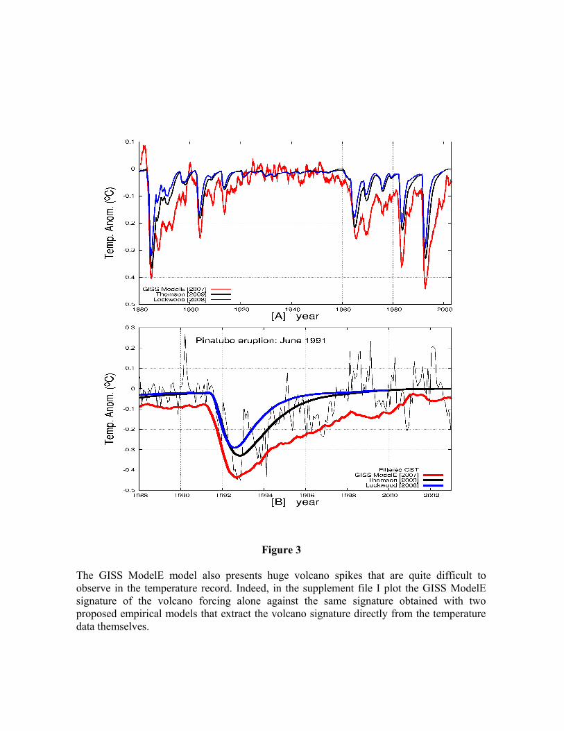
Figure 3

The GISS ModelE model also presents huge volcano spikes that are quite difficult to observe in the temperature record. Indeed, in the supplement file I plot the GISS ModelE signature of the volcano forcing alone against the same signature obtained with two proposed empirical models that extract the volcano signature directly from the temperature data themselves.

The figure clearly shows that the GISS ModelE computer model greatly overestimates the volcano cooling signature. The same is true for the other GCMs, as shown in the supplement file of the paper. This issue is quite important, as I will explain later. In fact, there exists an attempt to reconstruct climate variations by stressing the climatic effect of the volcano aerosol, but the lack of strong volcano spikes in the temperature record suggests that the volcano effect is already overestimated.

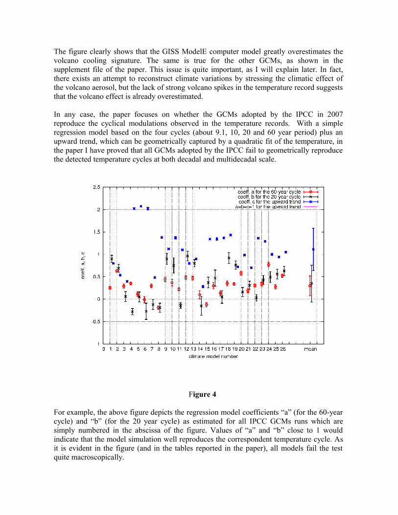
In any case, the paper focuses on whether the GCMs adopted by the IPCC in 2007 reproduce the cyclical modulations observed in the temperature records. With a simple regression model based on the four cycles (about 9.1, 10, 20 and 60 year period) plus an upward trend, which can be geometrically captured by a quadratic fit of the temperature, in the paper I have proved that all GCMs adopted by the IPCC fail to geometrically reproduce the detected temperature cycles at both decadal and multidecadal scale.

Figure 4

For example, the above figure depicts the regression model coefficients “a” (for the 60-year cycle) and “b” (for the 20 year cycle) as estimated for all IPCC GCMs runs which are simply numbered in the abscissa of the figure. Values of “a” and “b” close to 1 would indicate that the model simulation well reproduces the correspondent temperature cycle. As it is evident in the figure (and in the tables reported in the paper), all models fail the test quite macroscopically.

The conclusion is evident, simple and straightforward: all GCMs adopted by the IPCC fail in correctly reproducing the decadal and multidecadal dynamical modulation observed in the global surface temperature record, thus they do not reproduce the observed dynamics of the climate. Evidently, the “science is settled” claim is false. Indeed, the models are missing important physical mechanisms driving climate changes, which may also be still quite mysterious and which I believe to ultimately be astronomical induced, as better explained in my other papers.

But now, what can we do with this physical information?

It is important to realize that the “science is settled” claim is a necessary prerequisite for efficiently engineering any physical system with an analytical computer model, as the GCMs want to do for the climate system. If the science is not settled, however, such an engineering task is not efficient and theoretically impossible. For example, an engineer can not build a functional electric devise (a phone or a radio or a TV or a computer), or a bridge or an airplane if some of the necessary physical mechanisms were unknown. Engineering does not really work with a partial science, usually. In medicine, for example, nobody claims to cure people by using some kind of physiological GCM! And GCM computer modelers are essentially climate computer engineers more than climate scientists.

In theoretical science, however, people can attempt to overcome the above problem by using a different kind of models, the empirical/phenomenological ones, which have their own limits, but also numerous advantages. There is just the need to appropriately extract and use the information contained in the data themselves to model the observed dynamics.

Well, in the paper I used the geometrical information deduced from the temperature data to do two things:

1) I propose a correction of the proposed net anthropogenic warming effect on the climate

2) I implement the above net anthropogenic warming effect in the harmonic model to produce an approximate forecast for the 21st century global surface temperature by assuming the same IPCC emission projections.

To solve the first point we need to adopt a subtle reasoning. In fact, it is not possible to directly solve the natural versus the anthropogenic component of the upward warming trend observed in the climate since 1850 (about 0.8 °C) by using the harmonic model calibrated on the same data because with 161 years of data at most a 60-year cycle can be well detected, but not longer cycles.

Indeed, what numerous papers have shown, including some of mine, for examplehttp://www.sciencedirect.com/science/article/pii/S1364682609002089 , is that this 1850-2010 upward warming trend can be part of a multi-secular/millenarian natural cycle, which was also responsible for the Roman warming period, the Dark Ages, the Medieval Warm Period and the Little Ica Age.

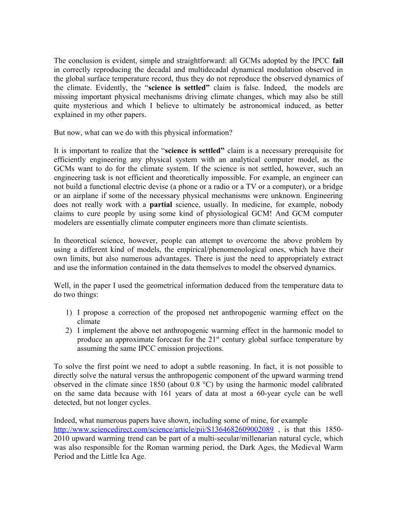
The following figure from Hulum et al. (2011), http://www.sciencedirect.com/science/article/pii/S0921818111001457 ,

Figure 5

gives an idea of how these multi-secular/millenarian natural cycles may appear by attempting a reconstruction of a pluri-millennial record proxy model for the temperature in central Greenland.

However, an accurate modeling of the multi-secular/millenarian natural cycles is not currently possible. The frequencies, amplitudes and phases are not known with great precision because the proxy models of the temperature look quite different from each other. Essentially, for our study, we want only to use the real temperature data and these data start in 1850, which evidently is a too short record for extracting multi-secular/millenarian natural cycles.

To proceed I have adopted a strategy based on the 60-year cycle, which has been estimate to have amplitude of about 0.3 °C, as the first figure above shows.

To understand the reasoning a good start is the IPCC’s figures 9.5a and 9.5b which are particularly popular among the anthropogenic global warming (AGW) advocates: http://www.ipcc.ch/publications_and_data/ar4/wg1/en/figure-9-5.html

These two figures are reproduced below:

Figure 6

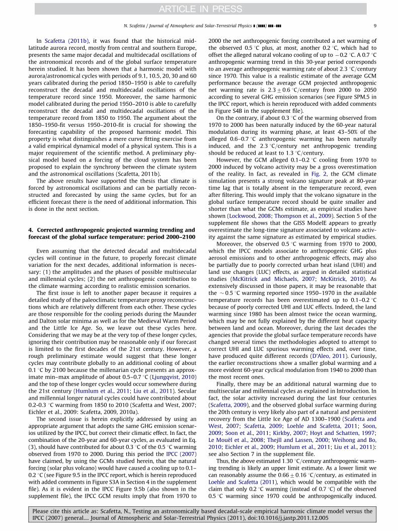
The above figure b shows that without anthropogenic forcing, according to the IPCC, the climate had to cool from 1970 to 2000 by about 0.0-0.2 °C because of volcano activity. Only the addition of anthropogenic forcings (see figure a) could have produced the 0.5 °C warming observed from 1970 to 2000. Thus, from 1970 to 2000 anthropogenic forcings are claimed to have produced a warming of about 0.5-0.7 °C in 30 years. This warming is then

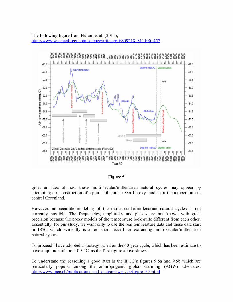
extended in the IPCC GCMs' projections for the 21st century with an anthropogenic warming trend of about 2.3 °C/century, as evident in the IPCC’s figure SPM5 shown belowhttp://www.ipcc.ch/publications_and_data/ar4/wg1/en/figure-spm-5.html

Figure 7

But our trust on this IPCC’s estimate of the anthropogenic warming effect is directly challenged by the failure of these GCMs in reproducing the 60-year natural modulation which is responsible for at least about 0.3 °C of warming from 1970 to 2000. Consequently, when taking into account this natural variability, the net anthropogenic warming effect should not be above 0.2-0.4 °C from 1970 to 2000, instead of the IPCC claimed 0.5-0.7 °C.

This implies that the net anthropogenic warming effect must be reduced to a maximum within a range of 0.5-1.3 °C/century since 1970 to about 2050 by taking into account the same IPCC emission projections, as argued in the paper. In the paper this result is reached by taking also into account several possibilities including the fact that the volcano cooling is evidently overestimated in the GCMs, as we have seen above, and that part of the leftover warming from 1970 to 2000 could have still be due to other factors such as urban heat island and land use change.

At this point it is possible to attempt a full forecast of the climate since 2000 that is made of the four detected decadal and multidecadal cycles plus the corrected anthropogenic warming effect trending. The results are depicted in the figures below

Figure 8

The figure shows a full climate forecast of my proposed empirical model, against the IPCC projections since 2000. It is evident that my proposed model agrees with the data much better than the IPCC projections, as also other tests present in the paper show.

My proposed model shows two curves: one is calibrated during the period 1850-1950 and the other is calibrated during the period 1950-2010. It is evident that the two curves equally well reconstruct the climate variability from 1850 to 2011 at the decadal /multidecadal scales, as the gray temperature smooth curve highlights, with an average error of just 0.05 °C.

The proposed empirical model would suggest that the same IPCC projected anthropogenic emissions imply a global warming by about 0.3–1.2 °C by 2100, in opposition to the IPCC

1.0–3.6 °C projected warming. My proposed estimate also excludes an additional possible cooling that may derive from the multi-secular/millennial cycle.

Some implicit evident consequences of this finding is that, for example, the ocean may rise quite less, let us say a third (about 5 inches/12.5 cm) by 2100, than what has been projected by the IPCC, and that we probably do not need to destroy our economy to attempt to reduce CO2 emissions. Will my forecast curve work, hopefully, for at least a few decades? Well, my model is not a “oracle crystal ball”. As it happens for the ocean tides, numerous other natural cycles may be present in the climate system at all time scales and may produce interesting interference patterns and a complex dynamics. Other nonlinear factors may be present as well, and sudden events such as volcano eruptions can always disrupt the dynamical pattern for a while. So, the model can be surely improved.

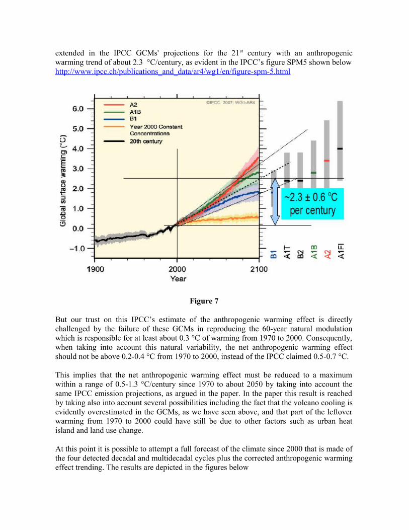
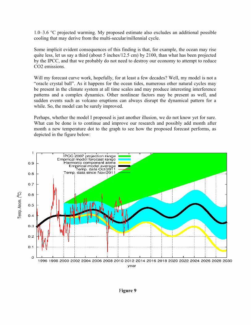
Perhaps, whether the model I proposed is just another illusion, we do not know yet for sure. What can be done is to continue and improve our research and possibly add month after month a new temperature dot to the graph to see how the proposed forecast performs, as depicted in the figure below:

Figure 9

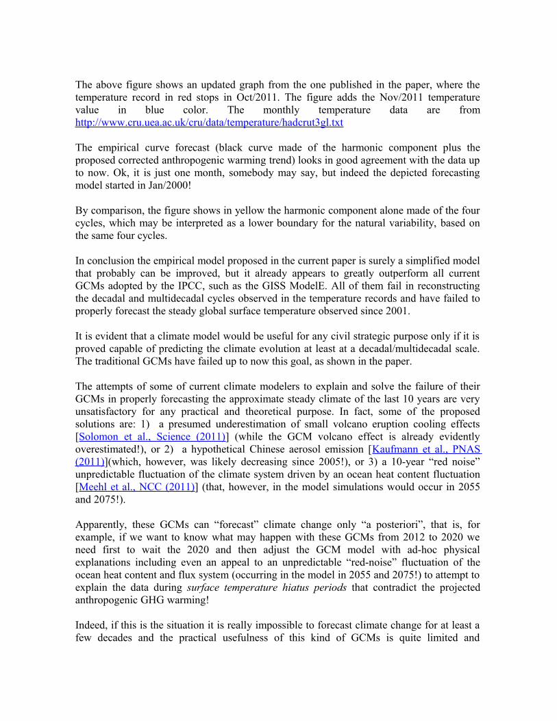
The above figure shows an updated graph from the one published in the paper, where the temperature record in red stops in Oct/2011. The figure adds the Nov/2011 temperature value in blue color. The monthly temperature data are from http://www.cru.uea.ac.uk/cru/data/temperature/hadcrut3gl.txt

The empirical curve forecast (black curve made of the harmonic component plus the proposed corrected anthropogenic warming trend) looks in good agreement with the data up to now. Ok, it is just one month, somebody may say, but indeed the depicted forecasting model started in Jan/2000!

By comparison, the figure shows in yellow the harmonic component alone made of the four cycles, which may be interpreted as a lower boundary for the natural variability, based on the same four cycles.

In conclusion the empirical model proposed in the current paper is surely a simplified model that probably can be improved, but it already appears to greatly outperform all current GCMs adopted by the IPCC, such as the GISS ModelE. All of them fail in reconstructing the decadal and multidecadal cycles observed in the temperature records and have failed to properly forecast the steady global surface temperature observed since 2001.

It is evident that a climate model would be useful for any civil strategic purpose only if it is proved capable of predicting the climate evolution at least at a decadal/multidecadal scale. The traditional GCMs have failed up to now this goal, as shown in the paper.

The attempts of some of current climate modelers to explain and solve the failure of their GCMs in properly forecasting the approximate steady climate of the last 10 years are very unsatisfactory for any practical and theoretical purpose. In fact, some of the proposed solutions are: 1) a presumed underestimation of small volcano eruption cooling effects [Solomon et al., Science (2011)] (while the GCM volcano effect is already evidently overestimated!), or 2) a hypothetical Chinese aerosol emission [Kaufmann et al., PNAS (2011)](which, however, was likely decreasing since 2005!), or 3) a 10-year “red noise” unpredictable fluctuation of the climate system driven by an ocean heat content fluctuation [Meehl et al., NCC (2011)] (that, however, in the model simulations would occur in 2055 and 2075!).

Apparently, these GCMs can “forecast” climate change only “a posteriori”, that is, for example, if we want to know what may happen with these GCMs from 2012 to 2020 we need first to wait the 2020 and then adjust the GCM model with ad-hoc physical explanations including even an appeal to an unpredictable “red-noise” fluctuation of the ocean heat content and flux system (occurring in the model in 2055 and 2075!) to attempt to explain the data during surface temperature hiatus periods that contradict the projected anthropogenic GHG warming!

Indeed, if this is the situation it is really impossible to forecast climate change for at least a few decades and the practical usefulness of this kind of GCMs is quite limited and

potentially very misleading because the model can project a 10-year warming while then the “red-noise” dynamics of the climate system completely changes the projected pattern!

The fact is that the above ad-hoc explanations appear to be in conflict with dynamics of the climate system as evident since 1850. Indeed, this dynamics suggests a major multiple harmonic influence component on the climate with a likely astronomical origin (sun + moon + planets) although not yet fully understood in its physical mechanisms, that, as shown in the above figures, can apparently explain also the post 2000 climate quite satisfactorily (even by using my model calibrated from 1850 to 1950, that is more than 50 years before the observed temperature hiatus period since 2000!).

Perhaps, a new kind of climate models based, at least in part, on empirical reconstruction of the climate constructed on empirically detected natural cycles may indeed perform better, may have better predicting capabilities and, consequently, may be found to be more beneficial to the society than the current GCMs adopted by the IPCC.

So, is a kind of Copernican Revolution needed in climate change research, as Alan Carlin has also suggested? http://www.carlineconomics.com/archives/1456

I personally believe that there is an urgent necessity of investing more funding in scientific methodologies alternative to the traditional GCM approach and, in general, to invest more in pure climate science research than just in climate GCM engineering research as done until now on the false claim that there is no need in investing in pure science because the “science is already settled”. About the other common AGW slogan according to which the current mainstream AGW climate science cannot be challenged because it has been based on the so-called “scientific consensus,” I would strongly suggest the reading of this post by Kevin Rice at the blog Catholibertarian entitled “On the dangerous naivety of uncritical acceptance of the scientific consensus”

http://catholibertarian.com/2011/12/30/on-the-dangerous-naivete-of-uncritical-acceptance-of-the-scientific-consensus/

It is a very educational and open-mind reading, in my opinion.

Nicola Scafetta, Ph.D.Duke UniversityDurham, [email protected]://www.fel.duke.edu/~scafetta/

Testing an astronomically-based decadal-scale empirical harmonic climate model versus the IPCC (2007) general circulation climate models

Nicola Scafetta ACRIM (Active Cavity Radiometer Solar Irradiance Monitor Lab) & Duke University, Durham, NC 27708, USA.

Journal of Atmospheric and Solar-Terrestrial Physics, (2011) doi:10.1016/j.jastp.2011.12.005

http://www.sciencedirect.com/science/article/pii/S1364682611003385

Testing an astronomically based decadal-scale empirical harmonic climatemodel versus the IPCC (2007) general circulation climate models

Nicola Scafetta n

ACRIM (Active Cavity Radiometer Solar Irradiance Monitor Lab) & Duke University, Durham, NC 27708, USA

a r t i c l e i n f o

Article history:

Received 1 August 2011

Received in revised form

9 December 2011

Accepted 10 December 2011

Keywords:

Solar variability

Planetary motion

Climate change

Climate models

a b s t r a c t

We compare the performance of a recently proposed empirical climate model based on astronomical

harmonics against all CMIP3 available general circulation climate models (GCM) used by the IPCC

(2007) to interpret the 20th century global surface temperature. The proposed astronomical empirical

climate model assumes that the climate is resonating with, or synchronized to a set of natural

harmonics that, in previous works (Scafetta, 2010b, 2011b), have been associated to the solar system

planetary motion, which is mostly determined by Jupiter and Saturn. We show that the GCMs fail to

reproduce the major decadal and multidecadal oscillations found in the global surface temperature

record from 1850 to 2011. On the contrary, the proposed harmonic model (which herein uses cycles

with 9.1, 10–10.5, 20–21, 60–62 year periods) is found to well reconstruct the observed climate

oscillations from 1850 to 2011, and it is shown to be able to forecast the climate oscillations from 1950

to 2011 using the data covering the period 1850–1950, and vice versa. The 9.1-year cycle is shown to be

likely related to a decadal Soli/Lunar tidal oscillation, while the 10–10.5, 20–21 and 60–62 year cycles

are synchronous to solar and heliospheric planetary oscillations. We show that the IPCC GCM’s claim

that all warming observed from 1970 to 2000 has been anthropogenically induced is erroneous because

of the GCM failure in reconstructing the quasi 20-year and 60-year climatic cycles. Finally, we show

how the presence of these large natural cycles can be used to correct the IPCC projected anthropogenic

warming trend for the 21st century. By combining this corrected trend with the natural cycles, we show

that the temperature may not significantly increase during the next 30 years mostly because of the

negative phase of the 60-year cycle. If multisecular natural cycles (which according to some authors

have significantly contributed to the observed 1700–2010 warming and may contribute to an

additional natural cooling by 2100) are ignored, the same IPCC projected anthropogenic emissions

would imply a global warming by about 0.3–1.2 1C by 2100, contrary to the IPCC 1.0–3.6 1C projected

warming. The results of this paper reinforce previous claims that the relevant physical mechanisms that

explain the detected climatic cycles are still missing in the current GCMs and that climate variations at

the multidecadal scales are astronomically induced and, in first approximation, can be forecast.

& 2011 Elsevier Ltd. All rights reserved.

1. Introduction

Herein, we test the performance of a recently proposedastronomical-based empirical harmonic climate model (Scafetta,2010b, in press) against all general circulation climate models(GCMs) adopted by the IPCC (2007) to interpret climate changeduring the last century. A large supplement file with all GCMsimulations herein studied plus additional information is addedto this manuscript. A reader is invited to look at the figuresdepicting the single GCM runs there reported to have a feelingabout the performance of these models.

The astronomical harmonic model assumes that the climatesystem is resonating with or is synchronized to a set of naturalfrequencies of the solar system. The synchronicity between solarsystem oscillations and climate cycles has been extensivelydiscussed and argued in Scafetta (2010a,b, 2011b), and in thenumerous references cited in those papers. We used the velocityof the Sun relative to the barycenter of the solar system and arecord of historical mid-latitude aurora events. It was observedthat there is a good synchrony of frequency and phase betweenmultiple astronomical cycles with periods between 5 and 100years and equivalent cycles found in the climate system. We referto those works for details and statistical tests. The majorhypothesized mechanism is that the planets, in particular Jupiterand Saturn, induce solar or heliospheric oscillations that induceequivalent oscillations in the electromagnetic properties of the

Contents lists available at SciVerse ScienceDirect

journal homepage: www.elsevier.com/locate/jastp

Journal of Atmospheric and Solar-Terrestrial Physics

1364-6826/$ - see front matter & 2011 Elsevier Ltd. All rights reserved.

doi:10.1016/j.jastp.2011.12.005

n Tel.: þ1 919 660 2643.

E-mail addresses: [email protected], [email protected]

Please cite this article as: Scafetta, N., Testing an astronomically based decadal-scale empirical harmonic climate model versus theIPCC (2007) general.... Journal of Atmospheric and Solar-Terrestrial Physics (2011), doi:10.1016/j.jastp.2011.12.005

Journal of Atmospheric and Solar-Terrestrial Physics ] (]]]]) ]]]–]]]

upper atmosphere. The latter induces similar cycles in the cloudcover and in the terrestrial albedo forcing the climate to oscillatein the same way. The soli/lunar tidal cyclical dynamics alsoappears to play an important role in climate change at specificfrequencies.

This work focuses only on the major decadal and multidecadaloscillations of the climate system, as observed in the globalsurface temperature data since AD 1850. A more detailed discus-sion about the interpretation of the secular climate warmingtrending since AD 1600 can be found in Scafetta and West (2007)and in Scafetta (2009) and in numerous other references therecited. About the millenarian cycle since the Middle Age a discus-sion is present in Scafetta (2010a) where the relative contributionof solar, volcano and anthropogenic forcing is also addressed, andin the numerous references cited in the above three papers. Alsocorrelation studies between the secular trend of the temperatureand the geomagnetic aa-index, the sunspot number and the solarcycle length address the above issue and are quite numerous: forexample Hoyt and Schatten (1997), Sonnemann (1998), and Thejlland Lassen (2000). Thus, a reader interested in better under-standing the secular climate trending topic is invited to readthose papers. In particular, about the 0.8 1C warming trendingobserved since 1900 numerous empirical studies based on thecomparison between the past climate secular and multisecularpatterns and equivalent solar activity patterns have concludedthat at least 50–70% of the observed 20th century warming couldbe associated to the increase of solar activity observed since theMaunder minimum of the 17th century: for example see Scafettaand West (2007), Scafetta (2009), Loehle and Scafetta (2011),Soon (2009), Soon et al. (2011), Kirkby (2007), Hoyt and Schatten(1997), Le Mouel et al. (2008), Thejll and Lassen (2000), Weihongand Bo (2010), and Eichler et al. (2009). Moreover, Humlum et al.(2011) noted that the natural multisecular/milennial climatecycles observed during the late Holocene climate change clearlysuggest that the secular 20th century warming could be mostlydue to these longer natural cycles, which are also expected to coolthe climate during the 21th century. A similar conclusion hasbeen reached by another study focusing on the multisecular andmillennial cycles observed in the temperature in the central-eastern Tibetan Plateau during the past 2485 years (Liu et al.,2011). For the benefit of the reader, in Section 7 in the supple-ment file the results reported in two of the above papers are verybriefly presented to graphically support the above claims.

It is important to note that the above empirical results contrastgreatly with the GCM estimates adopted by the IPCC claiming thatmore than 90% of the warming observed since 1900 has beenanthropogenically induced (compare Figures 9.5a and b in the IPCCreport which are reproduced in Section 4 in the supplement file). Inthe above papers it has been often argued that the current GCMsmiss important climate mechanisms such as, for example, a modula-tion of the cloud system via a solar induced modulation of the cosmicray incoming flux, which would greatly amplify the climate sensi-tivity to solar changes by modulating the terrestrial albedo (Scafetta,2011b:; Kirkby, 2007; Svensmark, 1998, 2007; Shaviv, 2008).

In addition to a well-known decadal climate cycle commonlyassociated to the Schawbe solar cycle by numerous authors (Hoytand Schatten, 1997), several studies have emphasized that theclimate system is characterized by a quasi bi-decadal (from18 year to 22 year) oscillation and by a quasi 60-year oscillation(Stockton et al., 1983; Currie, 1984; Cook et al., 1997; Agnihotriand Dutta, 2003; Klyashtorin et al., 2009; Sinha et al., 2005;Yadava and Ramesh, 2007; Jevrejeva et al., 2008; Knudsen et al.,2011; Davis and Bohling, 2001; Scafetta, 2010b; Weihong and Bo,2010; Mazzarella and Scafetta, 2011; Scafetta, in press). Forexample, quasi 20-year and 60-year large cycles are clearlydetected in all global surface temperature instrumental records

of both hemispheres since 1850 as well as in numerous astro-nomical records. There is a phase synchronization between theseterrestrial and astronomical cycles. As argued in Scafetta (2010b),the observed quasi bidecadal climate cycle may also be around a21-year periodicity because of the presence of the 22-year solarHale magnetic cycle, and there may also be an additionalinfluence of the 18.6-year soli/lunar nodal cycle. However, forthe purpose of the present paper, we can ignore these correctionswhich may require other cycles at 18.6 and 22 years. In the sameway, we ignore other possible slight cycle corrections due to theinterference/resonance with other planetary tidal cycles andwith the 11-year and 22-year solar cycles, which are left toanother study.

About the 60-year cycle it is easy to observe that the globalsurface temperature experienced major maxima in 1880–1881,1940–1941 and 2000–2001. These periods occurred during theJupiter/Saturn great conjunctions when the two planets werequite close to the Sun and the Earth. This events occur every threeJ/S synodic cycles. Other local temperature maxima occurredduring the other J/S conjunctions, which occur every about 20years: see Figures 10 and 11 in Scafetta (2010b), where thiscorrespondence is shown in details through multiple filtering ofthe data. Moreover, the tides produced by Jupiter and Saturn inthe heliosphere and in the Sun have a period of about0:5=ð1=11:86�1=29:45Þ � 10 years plus the 11.86-year Jupiterorbital tidal cycles. The two tides beat generating an additionalcycle at about 1=ð2=19:86�1=11:86Þ ¼ 61 years (Scafetta, inpress). Indeed, a quasi 60-year climatic oscillations have likelyan astronomical origin because the same cycles are found innumerous secular and millennial aurora and other solar relatedrecords (Charvatova et al., 1988; Komitov, 2009; Ogurtsov et al.,2002; Patterson et al., 2004; Yu et al., 1983; Scafetta, 2010a,b,2011b; Mazzarella and Scafetta, 2011).

A 60-year cycle is even referenced in ancient Sanskrit textsamong the observed monsoon rainfall cycles (Iyengar, 2009), a factconfirmed by modern monsoon studies (Agnihotri and Dutta, 2003).It is also observed in the sea level rise since 1700 (Jevrejeva et al.,2008) and in numerous ocean and terrestrial records for centuries(Klyashtorin et al., 2009). A natural 60-year climatic cycle associatedto planetary astronomical cycles may also explain the origin of 60-year cyclical calendars adopted in traditional Chinese, Tamil andTibetan civilizations (Aslaksen, 1999). Indeed, all major ancientcivilizations knew about the 20-year and 60-year astronomicalcycles associated to Jupiter and Saturn (Temple, 1998).

In general, power spectrum evaluations have shown thatfrequency peaks with periods of about 9.1, 10–10.5, 20–22 and60–63 years are the most significant ones and are commonbetween astronomical and climatic records (Scafetta, 2010b, inpress). Evidently, if climate is described by a set of harmonics, itcan be in first approximation reconstructed and forecast by usinga planetary harmonic constituent analysis methodology similar tothe one that was first proposed by Lord Kelvin (Thomson, 1881;Scafetta, in press) to accurately reconstruct and predict tidaldynamics. The harmonic constituent model is just a superpositionof several harmonic terms of the type

FðtÞ ¼ A0þXN

i ¼ 1

Ai cosðoitþfiÞ, ð1Þ

whose frequencies oi are deduced from the astronomical theoriesand the amplitude Ai and phase fi of each harmonic constituentare empirically determined using regression on the available data,and then the model is used to make forecasts. Several harmonicsare required: for example, most locations in the United States usecomputerized forms of Kelvin’s tide-predicting machine with35–40 harmonic constituents for predicting local tidal amplitudes

N. Scafetta / Journal of Atmospheric and Solar-Terrestrial Physics ] (]]]]) ]]]–]]]2

Please cite this article as: Scafetta, N., Testing an astronomically based decadal-scale empirical harmonic climate model versus theIPCC (2007) general.... Journal of Atmospheric and Solar-Terrestrial Physics (2011), doi:10.1016/j.jastp.2011.12.005

(Ehret, 2008), so a reader should not be alarmed if many harmonicconstituents may be needed to accurately reconstruct the climatesystem.

Herein we show that a similar harmonic empirical methodologycan, in first approximation, reconstruct and forecast global climatechanges at least on a decadal and multidecadal scales, and that thismethodology works much better than the current GCMs adopted bythe IPCC (2007). In fact, we will show that the IPCC GCMs fail toreproduce the observed climatic oscillations at multiple temporalscales. Thus, the computer climate models adopted by the IPCC(2007) are found to be missing the important physical mechanismsresponsible for the major observed climatic oscillations. An impor-tant consequence of this finding is that these GCMs have seriouslymisinterpreted the reality by significantly overestimating theanthropogenic contribution, as also other authors have recentlyclaimed (Douglass et al., 2007; Lindzen and Choi, 2011; Spencer andBraswell, 2011). Consequently, the IPCC projections for the 21stcentury should not be trusted.

2. The IPCC GCMs do not reproduce the global surfacetemperature decadal and multidecadal cycles

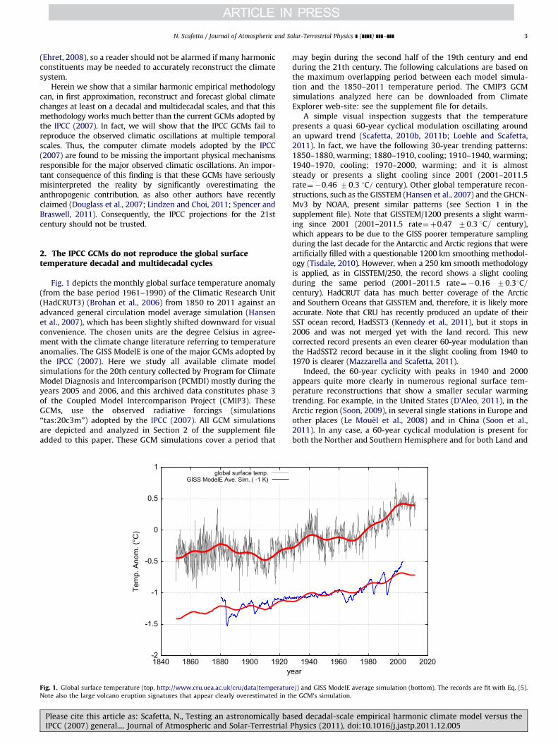
Fig. 1 depicts the monthly global surface temperature anomaly(from the base period 1961–1990) of the Climatic Research Unit(HadCRUT3) (Brohan et al., 2006) from 1850 to 2011 against anadvanced general circulation model average simulation (Hansenet al., 2007), which has been slightly shifted downward for visualconvenience. The chosen units are the degree Celsius in agree-ment with the climate change literature referring to temperatureanomalies. The GISS ModelE is one of the major GCMs adopted bythe IPCC (2007). Here we study all available climate modelsimulations for the 20th century collected by Program for ClimateModel Diagnosis and Intercomparison (PCMDI) mostly during theyears 2005 and 2006, and this archived data constitutes phase 3of the Coupled Model Intercomparison Project (CMIP3). TheseGCMs, use the observed radiative forcings (simulations‘‘tas:20c3m’’) adopted by the IPCC (2007). All GCM simulationsare depicted and analyzed in Section 2 of the supplement fileadded to this paper. These GCM simulations cover a period that

may begin during the second half of the 19th century and endduring the 21th century. The following calculations are based onthe maximum overlapping period between each model simula-tion and the 1850–2011 temperature period. The CMIP3 GCMsimulations analyzed here can be downloaded from ClimateExplorer web-site: see the supplement file for details.

A simple visual inspection suggests that the temperaturepresents a quasi 60-year cyclical modulation oscillating aroundan upward trend (Scafetta, 2010b, 2011b; Loehle and Scafetta,2011). In fact, we have the following 30-year trending patterns:1850–1880, warming; 1880–1910, cooling; 1910–1940, warming;1940–1970, cooling; 1970–2000, warming; and it is almoststeady or presents a slight cooling since 2001 (2001–2011.5rate¼�0.46 70:3 1C= century). Other global temperature recon-structions, such as the GISSTEM (Hansen et al., 2007) and the GHCN-Mv3 by NOAA, present similar patterns (see Section 1 in thesupplement file). Note that GISSTEM/1200 presents a slight warm-ing since 2001 (2001–2011.5 rate¼þ0.47 70:3 1C= century),which appears to be due to the GISS poorer temperature samplingduring the last decade for the Antarctic and Arctic regions that wereartificially filled with a questionable 1200 km smoothing methodol-ogy (Tisdale, 2010). However, when a 250 km smooth methodologyis applied, as in GISSTEM/250, the record shows a slight coolingduring the same period (2001–2011.5 rate¼�0.16 70:31C=century). HadCRUT data has much better coverage of the Arcticand Southern Oceans that GISSTEM and, therefore, it is likely moreaccurate. Note that CRU has recently produced an update of theirSST ocean record, HadSST3 (Kennedy et al., 2011), but it stops in2006 and was not merged yet with the land record. This newcorrected record presents an even clearer 60-year modulation thanthe HadSST2 record because in it the slight cooling from 1940 to1970 is clearer (Mazzarella and Scafetta, 2011).

Indeed, the 60-year cyclicity with peaks in 1940 and 2000appears quite more clearly in numerous regional surface tem-perature reconstructions that show a smaller secular warmingtrending. For example, in the United States (D’Aleo, 2011), in theArctic region (Soon, 2009), in several single stations in Europe andother places (Le Mouel et al., 2008) and in China (Soon et al.,2011). In any case, a 60-year cyclical modulation is present forboth the Norther and Southern Hemisphere and for both Land and

-2

-1.5

-1

-0.5

0

0.5

1

1840 1860 1880 1900 1920 1940 1960 1980 2000 2020

Tem

p. A

nom

. (°C

)

year

global surface temp.GISS ModelE Ave. Sim. ( -1 K)

Fig. 1. Global surface temperature (top, http://www.cru.uea.ac.uk/cru/data/temperature/) and GISS ModelE average simulation (bottom). The records are fit with Eq. (5).

Note also the large volcano eruption signatures that appear clearly overestimated in the GCM’s simulation.

N. Scafetta / Journal of Atmospheric and Solar-Terrestrial Physics ] (]]]]) ]]]–]]] 3

Please cite this article as: Scafetta, N., Testing an astronomically based decadal-scale empirical harmonic climate model versus theIPCC (2007) general.... Journal of Atmospheric and Solar-Terrestrial Physics (2011), doi:10.1016/j.jastp.2011.12.005

Ocean regions (Scafetta, 2010b) even if it may be partially hiddenby the upward warming trending. The 60-year modulationappears well correlated to a recently proposed solar activityreconstruction (Loehle and Scafetta, 2011).

The 60-year cyclical modulation of the temperature from 1850to 2011 is further shown in Fig. 2 where the autocorrelationfunctions of the global surface temperature and of the GISSModelE average simulation are compared. The autocorrelationfunction is defined as

rðtÞ ¼PN�t

t ¼ 1ðTt�T ÞðTtþt�T ÞffiffiffiffiffiffiffiffiffiffiffiffiffiffiffiffiffiffiffiffiffiffiffiffiffiffiffiffiffiffiffiffiffiffiffiffiffiffiffiffiffiffiffiffiffiffiffiffiffiffiffiffiffiffiffiffiffiffiffiffiffiffiffiffiffiPN�tt ¼ 1ðTt�T Þ2

PNt ¼ tðTt�T Þ2

h ir , ð2Þ

where T is the average of the N-data long temperature record andt is the time-lag. The autocorrelation function of the globalsurface temperature (Fig. 2A) and of the same record detrendedof its quadratic trend (Fig. 2B) reveals the presence of a clearcyclical pattern with minima at about 30-year lag and 90-year lag,and maxima at about 0-year lag and 60-year lag. This patternindicates the presence of a quasi 60-year cyclical modulation inthe record. Moreover, because both figures show the same patternit is demonstrated that the quadratic trend does not artificiallycreates the 60-year cyclicity. On the contrary, the GISS ModelEaverage simulation produces a very different autocorrelationpattern lacking any cyclical modulation. Fig. 2C shows the auto-correlation function of the two records detrended also of their

-0.4

-0.2

0

0.2

0.4

0.6

0.8

1

auto

corr

elat

ion

func

tion

[A] time-lag (year)

-0.6

-0.4

-0.2

0

0.2

0.4

0.6

0.8

auto

corr

elat

ion

func

tion

[B] time-lag (year)

-0.4

-0.2

0

0.2

0.4

0.6

0.8

0 10 20 30 40 50 60 70 80 90 100

auto

corr

elat

ion

func

tion

[C] time-lag (year)

0 10 20 30 40 50 60 70 80 90 100

0 10 20 30 40 50 60 70 80 90 100

Fig. 2. Autocorrelation function (Eq. (2)) of the global surface temperature and of the GISS ModelE average simulation: [A] original data; [B] data detrended of their

quadratic fit; [C] the 60-year modulation is further detrended. Note the 60-year cyclical modulation of the autocorrelation of the temperature with minima at 30-year and

90-year lags and maxima at 0-year and 60-year lags, which is not reproduced by the GCM simulation. Moreover, the computer simulation presents an autocorrelation peak

at 80-year lag related to a pattern produced by volcano eruptions, which is absent in the temperature. See Section 5 in the supplement file for further evidences about the

GISS ModelE serious overestimation of the volcano signal in the global surface temperature record.

N. Scafetta / Journal of Atmospheric and Solar-Terrestrial Physics ] (]]]]) ]]]–]]]4

Please cite this article as: Scafetta, N., Testing an astronomically based decadal-scale empirical harmonic climate model versus theIPCC (2007) general.... Journal of Atmospheric and Solar-Terrestrial Physics (2011), doi:10.1016/j.jastp.2011.12.005

60-year cyclical fit, and the climatic record appears to becharacterized by a quasi 20-year smaller cycle, as deduced bythe small but visible quasi regular 20-year waves, at least up to atime-lag of 70 years after which other faster oscillations with adecadal scale dominate the pattern. On the contrary, the auto-correlation function of the GCM misses both the decadal and bi-decadal oscillations and again shows a strong 80-year lag peak,absent in the temperature. The latter peak is due to the quasi80-year lag between the two computer large volcano eruptionsignatures of Krakatoa (1883) and Agung (1963–1964), and to thequasi 80-year lag between the volcano signatures of Santa Maria(1902) and El Chichon (1982). Because this 80-year lag autocor-relation peak is not evident in the autocorrelation function of theglobal temperature we can conjecture that the GISS ModelE issignificantly overestimating the volcano signature, in addition tonot reproducing the natural decadal and multidecadal tempera-ture cycles: this claim is further supported in Section 5 of thesupplement file.

A similar qualitative conclusion applies also to all other GCMsused by the IPCC, as shown in Section 2 of the supplement file.The single GCM runs as well as their average reconstructionsappear quite different from each other: some of them are quiteflat until 1970, others are simply monotonically increasing.Volcano signals often appear overestimated. Finally, althoughthese GCM simulations present some kind of red-noise variabilitysupposed to simulate the multi-annual, decadal and multidecadalnatural variability, a simple visual comparison among the simula-tions and the temperature record gives a clear impression that thesimulated variability has nothing to do with the observed tem-perature dynamics. In conclusion, a simple visual analysis of therecords suggests that the temperature is characterized 10-year,20-year and 60-year oscillations that are simply not reproducedby the GCMs. This is also implicitly indicated by the very smoothand monotonically increasing pattern of their average reconstruc-tion depicted in the IPCC figure SPM.5 (see Section 4 in thesupplement file).

1e-005

0.0001

0.001

0.01 ~9.1

~10/10.5

~20/21 ~60/62

0.1

1

10 100

PS (g

ener

ic u

nits

)

[A] 1/f, period (year)

period 1850-2011

MEM M=968 (the data are not linearly detrended)Lomb Periodogram (the data are linearly detrended)

0.0001

0.001

0.01

0.1

1

10

100

10 100

PS (g

ener

ic u

nits

)

[B] 1/f, period (year)

MEM M=790 (top), Lomb Periodogram (bottom)period 1880-2011

HadCRUT3GISSTEM/250

GHCN-Mv3

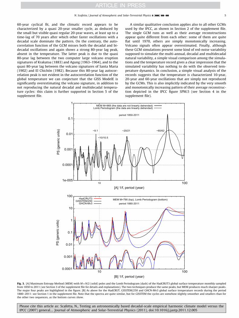
Fig. 3. [A] Maximum Entropy Method (MEM) with M¼N/2 (solid) poles and the Lomb Periodogram (dash) of the HadCRUT3 global surface temperature monthly sampled

from 1850 to 2011 (see Section 3 of the supplement file for details and explanations). The two techniques produce the same peaks, but MEM produces much sharper peaks.

The major four peaks are highlighted in the figure. [B] As above for the HadCRUT, GISSTEM/250 and GHCN-Mv3 global surface temperature records during the period

1880–2011: see Section 1 in the supplement file. Note that the spectra are quite similar, but for GISSTEM the cycles are somehow slightly smoother and smallers than for

the other two sequences, as the bottom curves show.

N. Scafetta / Journal of Atmospheric and Solar-Terrestrial Physics ] (]]]]) ]]]–]]] 5

Please cite this article as: Scafetta, N., Testing an astronomically based decadal-scale empirical harmonic climate model versus theIPCC (2007) general.... Journal of Atmospheric and Solar-Terrestrial Physics (2011), doi:10.1016/j.jastp.2011.12.005

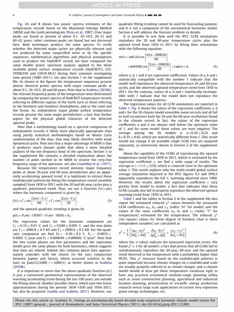
Fig. 3A and B shows two power spectra estimates of thetemperature records based on the Maximum Entropy Method(MEM) and the Lomb periodogram (Press et al., 2007). Four majorpeaks are found at periods of about 9.1, 10–10.5, 20–21 and60–62 years: other common peaks are found but not discussedhere. Both techniques produce the same spectra. To verifywhether the detected major cycles are physically relevant andnot produced by some unspecified noise or by the specificsequences, mathematical algorithms and physical assumptionsused to produce the HadCRUT record, we have compared thesame double power spectrum analysis applied to the threeavailable global surface temperature records (HadCRUT3, GIS-STEM/250 and GHCN-Mv3) during their common overlappingtime period (1880–2011): see also Section 1 in the supplementfile. As shown in the figures the temperature sequences presentalmost identical power spectra with major common peaks atabout 9.1, 10–10.5, 20 and 60 years. Note that in Scafetta (2010b),the relevant frequency peaks of the temperature were determinedby comparing the power spectra of HadCRUT temperature recordsreferring to different regions of the Earth such as those referringto the Northern and Southern hemispheres, and to the Land andthe Ocean. So, independent major global surface temperaturerecords present the same major periodicities: a fact that furtherargues for the physical global character of the detectedspectral peaks.

Note that a methodology based on a spectral comparison ofindependent records is likely more physically appropriate thanusing purely statistical methodologies based on Monte Carlorandomization of the data, that may likely interfere with weakdynamical cycles. Note also that a major advantage of MEM is thatit produces much sharper peaks that allow a more detailedanalysis of the low-frequency band of the spectrum. Section 5 inthe supplement file contains a detailed explanation about thenumber of poles needed to let MEM to resolve the very-lowfrequency range of the spectrum: see also Courtillot et al. (1977).

Because the temperature record presents major frequencypeaks at about 20-year and 60-year periodicities plus an appar-ently accelerating upward trend, it is legitimate to extract thesemultidecadal patterns by fitting the temperature record (monthlysampled) from 1850 to 2011 with the 20 and 60-year cycles plus aquadratic polynomial trend. Thus, we use a function f ðtÞþpðtÞ

where the harmonic component is given by

f ðtÞ ¼ C1 cos2pðt�T1Þ

60

� �þC2 cos

2pðt�T2Þ

20

� �, ð3Þ

and the upward quadratic trending is given by

pðtÞ ¼ P2nðt�1850Þ2þP1nðt�1850ÞþP0: ð4Þ

The regression values for the harmonic component areC1 ¼ 0:1070:01 1C and C2 ¼ 0:04070:005 1C, and the two datesare T1 ¼ 2000:870:5 AD and T2 ¼ 2000:870:5 AD. For the quad-ratic component we find P0 ¼�0:3070:2 1C, P1 ¼�0:003570:0005 1C=year and P2 ¼ 0:00004970:000002 1C=year2. Note thatthe two cosine phases are free parameters and the regressionmodel gives the same phases for both harmonics, which suggeststhat they are related. Indeed, this common phase date approxi-mately coincides with the closest (to the sun) conjunctionbetween Jupiter and Saturn, which occurred (relative to theSun) on June/23/2000 (� 2000:5), as better shown in Scafetta(2010b).

It is important to stress that the above quadratic function p(t)is just a convenient geometrical representation of the observedwarming accelerating trend during the last 160 years, not outsidethe fitting interval. Another possible choice, which uses two linearapproximations during the periods 1850–1950 and 1950–2011,has also be proposed (Loehle and Scafetta, 2011). However, our

quadratic fitting trending cannot be used for forecasting purpose,and it is not a component of the astronomical harmonic model.Section 4 will address the forecast problem in details.

It is possible to test how well the IPCC GCM simulationsreproduce the 20 and 60-year temperature cycles plus theupward trend from 1850 to 2011 by fitting their simulationswith the following equation:

mðtÞ ¼ an0:10 cos2pðt�2000:8Þ

60

� �

þbn0:040 cos2pðt�2000:8Þ

20

� �þcnpðtÞþd, ð5Þ

where a, b, c and d are regression coefficients. Values of a, b and c

statistically compatible with the number 1 indicate that themodel well reproduces the observed temperature 20 and 60-yearcycles, and the observed upward temperature trend from 1850 to2011. On the contrary, values of a, b and c statistically incompa-tible with 1 indicate that the model does not reproduce theobserved temperature patterns.

The regression values for all GCM simulations are reported inTable 1. Fig. 4 shows the values of the regression coefficients a, b

and c for the 26 climate model ensemble-mean records and all failto well reconstruct both the 20 and the 60-year oscillations foundin the climate record. In fact, the values of the regressioncoefficients a and b are always well below the optimum valueof 1, and for some model these values are even negative. Theaverage among the 26 models is a¼0.3070.22 andb¼0.3570.42, which are statistically different from 1. This resultwould not change if all available single GCM runs are analyzedseparately, as extensively shown in Section 2 of the supplementfile.

About the capability of the GCMs of reproducing the upwardtemperature trend from 1850 to 2011, which is estimated by theregression coefficient c, we find a wide range of results. Theaverage is c¼1.1170.50, which is centered close to the optimumvalue 1. This result explains why the multi-model global surfaceaverage simulation depicted in the IPCC figures 9.5 and SPM.5apparently reproduces the 0.8 1C warming observed since 1900.However, the results about the regression coefficient c varygreatly from model to model: a fact that indicates that theseGCMs usually also fail to properly reproduce the observed upwardwarming trend from 1850 to 2011.

Table 1 and the tables in Section 2 in the supplement file alsoreport the estimated reduced w2 values between the measuredGCM coefficients am, bm and cm (index ‘‘m’’ for model) and thevalues of the same coefficients aT, bT and cT (index ‘‘T’’ fortemperature) estimated for the temperature. The reduced w2

(chi square) values for three degree of freedom (that is threeindependent variables) are calculated as

w2 ¼1

3

ðam�aT Þ2

Da2mþDa2

T

þðbm�bT Þ

2

Db2mþDb2

T

þðcm�cT Þ

2

Dc2mþDc2

T

" #, ð6Þ

where the D values indicate the measured regression errors. Wefound w2

b1 for all models: a fact that proves that all GCMs fail tosimultaneously reproduce the 20-year, 60-year and the upwardtrend observed in the temperature with a probability higher than99.9%. This w2 measure based on the multidecadal patterns isquite important because climate changes on a multidecadal scaleare usually properly referred to as climate changes, and a climatemodel should at least get these temperature variations right tohave any practical economical medium-range planning utilitysuch as street construction planning, agricultural and industriallocation planning, prioritization of scientific energy productionresearch versus large scale applications of current very expensivegreen energy technologies, etc.

N. Scafetta / Journal of Atmospheric and Solar-Terrestrial Physics ] (]]]]) ]]]–]]]6

Please cite this article as: Scafetta, N., Testing an astronomically based decadal-scale empirical harmonic climate model versus theIPCC (2007) general.... Journal of Atmospheric and Solar-Terrestrial Physics (2011), doi:10.1016/j.jastp.2011.12.005

-1

-0.5

0

0.5

1

1.5

2

2.5

0 1 2 3 4 5 6 7 8 9 10 11 12 13 14 15 16 17 18 19 20 21 22 23 24 25 26 mean

coef

f. a,

b, c

climate model number

coeff. a for the 60-year cyclecoeff. b for the 20-year cyclecoeff. c for the upward trend

a=b=c=1 for the upward trend

Fig. 4. Values of the regression coefficients a, b and c relative to the amplitude of the 60 and 20-year cycles, and the upward trend obtained by regression fit of the 26 GCM

simulations of the 20th century used by the IPCC. See Table 1 and Section 2 in the supplement file for details. The result shows that all GCMs significantly fail in

reproducing the 20-year and 60-year cycle amplitudes observed in the temperature record by an average factor of 3.

Table 1Values of the regression parameters of Eq. (5) obtained by fitting the 25 IPCC (2007) climate GCM ensemble-mean estimates. #1 refers to the ensemble average of the GISS

ModelE depicted in Fig. 1a; #2–#26 refers to the 25 IPCC GCMs. Pictures and analysis concerning all 95 records including each single GCM run are shown in Section 2 in the

supplement file that accompanies this paper. The optimum value of these regression parameters should be a¼ b¼ c¼ 1 as presented in the first raw that refers to the

regression coefficients of the same model used to fit the temperature record. The last column refers to a reduced w2 test based on three coefficients a, b and c: see Eq. (6).

This determines the statistical compatibility of the regression coefficient measured for the GCM models and those observed in the temperature. It is always measured a

reduced w2b1 for three degrees of freedom, which indicates that the statistical compatibility of the GCMs with the observed 60-year, 20-year temperature cycles plus the

secular trending is less than 0.1%. These GCM regression values are depicted in Fig. 4: the regression coefficients for each available GCM simulation are reported in the

supplement file. The w2 test in the first line refers to the compatibility of the proposed model in Eq. (3) relative to the ideal case of a¼ b¼ c¼ 1 that gives a reduced

w2 ¼ 0:21 which imply that the statistical compatibility of Eq. (3) with the temperature cycles plus the secular trending is about 90%. The fit has been implemented using

the nonlinear least-squares (NLLS) Marquardt–Levenberg algorithm.

# Model a (60-year) b (20-year) c (trend) d (bias) w2 (abc)

Temp 1.0370.05 0.9970.12 1.0170.02 0.0070.01 0.21

1 GISS ModelE 0.2570.03 0.9070.08 0.8070.01 0.0870.01 89

2 BCC CM1 0.6370.03 0.6970.09 0.5470.02 0.0870.01 109

3 BCCR BCM2.0 0.2970.05 0.0670.11 0.4070.02 0.0870.01 202

4 CGCM3.1 (T47) 0.3570.03 �0.2870.07 2.0270.01 0.4070.01 753

5 CGCM3.1 (T63) 0.1170.05 0.0570.11 2.0770.02 0.4070.01 536

6 CNRM CM3 �0.0170.07 �0.2770.18 2.0270.03 0.3970.01 322

7 CSIRO MK3.0 0.3070.04 �0.1270.11 0.4870.02 0.0870.01 176

8 CSIRO MK3.5 �0.1970.04 �0.1970.10 1.3870.02 0.2570.01 197

9 GFDL CM2.0 0.4470.05 0.9070.12 1.1270.02 0.2170.01 28

10 GFDL CM2.1 0.3770.07 0.7570.17 1.3770.03 0.2670.01 53

11 GISS AOM 0.2270.03 �0.1470.06 1.1070.01 0.2270.01 93

12 GISS EH 0.4870.04 0.9670.11 0.8070.02 0.1470.01 43

13 GISS ER 0.4770.04 0.8070.08 0.9070.02 0.1170.01 31

14 FGOALS g1.0 0.1070.09 �0.1570.21 0.2870.03 0.0670.01 171

15 INVG ECHAM4 �0.1270.05 0.3770.12 1.3470.02 0.2470.01 138

16 INM CM3.0 0.3070.07 0.4770.18 1.3470.03 0.2470.01 54

17 IPSL CM4 0.1370.06 0.0570.14 1.3770.02 0.2670.01 107

18 MIROC3.2 Hires 0.3570.05 0.9270.12 1.4370.02 0.1970.01 104

19 MIROC3.2 Medres 0.3470.03 0.7670.09 0.7270.01 0.1470.01 104

20 ECHO G 0.5870.04 0.1670.10 0.9870.02 0.1870.01 26

21 ECHAM5/MPI-OM 0.1970.04 0.3170.09 0.7070.02 �0.0270.01 104

22 MRI CGCM 2.3.2 0.3170.03 0.0370.07 1.3670.01 0.2770.01 149

23 CCSM3.0 0.3470.04 0.4370.10 1.2970.02 0.2470.01 76

24 PCM 0.7770.05 0.4970.12 1.0070.02 0.1670.01 7

25 UKMO HADCM3 0.2870.05 0.5670.11 0.9470.02 0.1870.01 42

26 UKMO HADGEM1 0.5270.04 0.6370.10 1.0570.02 0.2070.01 24

Average 0.3070.22 0.3570.41 1.1170.47 0.1970.11 143.8

N. Scafetta / Journal of Atmospheric and Solar-Terrestrial Physics ] (]]]]) ]]]–]]] 7

Please cite this article as: Scafetta, N., Testing an astronomically based decadal-scale empirical harmonic climate model versus theIPCC (2007) general.... Journal of Atmospheric and Solar-Terrestrial Physics (2011), doi:10.1016/j.jastp.2011.12.005

It is also possible to include in the discussion the two detecteddecadal cycles as

gðtÞ ¼ C3 cos2pðt�T3Þ

10:44

� �þC4 cos

2pðt�T4Þ

9:07

� �: ð7Þ

A detailed discussion about the choice of the two above periodsand their physical meaning is better addressed in Section 4.Fitting the temperature for the period 1850–2011 givesC3 ¼ 0:0370:01 1C, T3 ¼ 2002:770:5 AD, C4 ¼ 0:0570:01 1C,T4 ¼ 1997:770:3 AD. It is possible to test how well the IPCCGCMs reconstruct these two decadal cycles by fitting theirsimulations with the following equation:

nðtÞ ¼mðtÞþsn0:03 cos2pðt�2002:7Þ

10:44

� �þ ln0:05 cos

2pðt�1997:7Þ

9:07

� �,

ð8Þ

where s and l are the regression coefficients. Values of s and l

statistically compatible with the number 1 indicate that themodel well reproduces the two observed decadal temperaturecycles, respectively. On the contrary, values of s and l statisticallyincompatible with 1 indicate that the model does not reproducethe observed temperature cycles. The results referring the averagemodel run, as defined above, are reported in Table 2, where it isevident that the GCMs fail to reproduce these two decadal cyclesas well. The average values among the 26 models is s¼0.0670.40and l¼0.3470.37, which are statistically different from 1. Inmany cases the regression coefficients are even negative. The

table also includes the reduced w2 (chi square) values for fivedegree of freedom by extending Eq. (6) to include the other twodecadal cycles. Again, we found w2

b1 for all models.Finally, we can estimate how well the astronomical model

made of the sum of the four harmonics plus the quadratic trend(that is f ðtÞþgðtÞþpðtÞ) reconstructs the 1850–2011 temperaturerecord relative to the GCM simulations. For this purpose weevaluate the root mean square (RMS) residual values betweenthe 4-year average smooth curves of each GCM average simula-tion and the 4-year average smooth of the temperature curve, andwe do the same between the astronomical model and the 4-yearaverage smooth temperature curve. We use a 4-year averagesmooth because the model is not supposed to reconstruct the fastsub-decadal fluctuations. The RMS residual values are reported inTable 2. The RMS residual value relative to the harmonic model is0.051 1C, while for the GCMs we get RMS residual values from 2 to5 times larger. This result further indicates that the geometricalmodel is significantly more accurate than the GCMs in recon-structing the global surface temperature from 1850 to 2011.

The above finding reinforces the conclusion of Scafetta (2010b)that the IPCC (2007) GCMs do not reproduce the observed majordecadal and multidecadal dynamical patterns observed in theglobal surface temperature record. This conclusion does notchange if the single GCM runs are studied.

3. Reconstruction of the global surface temperatureoscillations: 1880–2011

A regression model may always produce results in a reason-able agreement within the same time interval used for itscalibration. Thus, showing that an empirical model can recon-struct the same data used for determining its free regressionparameters would be not surprising, in general. However, if thesame model is shown to be capable of forecasting the patterns ofthe data outside the temporal interval used for its statisticalcalibration, then the model likely has a physical meaning. In fact,in the later case the regression model would be using construc-tors that are not simply independent generic mathematicalfunctions, but are functions that capture the dynamics of thesystem under study. Only a mathematical model that is shown tobe able to both reconstruct and forecast (or predict) the observa-tions is physically relevant according the scientific method.

The climate reconstruction efficiency of an empirical climatemodel based on a set of astronomical cycles with the periodsherein analyzed has been tested and verified in Scafetta (2010b, inpress) and Loehle and Scafetta (2011). Herein, we simply sum-marize some results for the benefit of the reader and for introdu-cing the following section.

In Figures 10 and 11 in Scafetta (2010b) it is shown that the20-year and 60-year oscillations of the speed of the Sun relative tothe barycenter of the solar system are in a very good phasesynchronization with the correspondent 20 and 60-year climateoscillations. Moreover, detailed spectra analysis has revealed thatthe climate system shares numerous other frequencies with theastronomical record.

In Figures 3 and 5 in Loehle and Scafetta (2011) it is shownthat an harmonic model based on 20-year and 60-year cycles andfree phases calibrated on the global surface temperature data forthe period 1850–1950 is able to properly reconstruct the 20-yearand 60-year modulation of the temperature observed since 1950.This includes a small peak around 1960, the cooling from 1940 to1970, the warming from 1970 to 2000 and a slight stable/coolingtrending since 2000. It was also found a quasi linear residual witha warming trending of about 0:6670:16 1C=century that wasinterpreted as due to a net anthropogenic warming trending.

Table 2Values of the regression parameters s and l of Eq. (8) obtained by fitting the 26

IPCC (2007) climate GCM ensemble-mean estimates. The fit has been implemen-

ted using the nonlinear least-squares (NLLS) Marquardt–Levenberg algorithm.

Note that the two regression coefficients are quite different from the optimum

values s¼ l¼ 1, as found for the temperature. The column referring to the reduced

w2 test is based on all five regression coefficients (a, b, c, s and l) by extending

Eq. (6). Again it is always observed a w2b1, which indicates incompatibility

between the GCM and the temperature patterns. The last column indicates the

RMS residual values between the 4-year average smooth curves of each GCM

simulation and the 4-year average smooth curve of the temperature: the value

associated to the first raw (temperature) RMS¼0.051 1C) refers to the RMS of the

astronomical harmonic model that suggests that the latter is statistically 2–5 times

more accurate than the GCM simulations in reconstructing the temperature record.

# Model s (10.44-year) l (9.1-year) w2 (abcsl) RMS (1C)

0 Temperature 1.0670.16 0.9970.10 0.15 0.051

1 GISS ModelE 0.3070.11 0.4070.07 61 0.107

2 BCC CM1 0.5370.11 0.4970.07 70 0.105

3 BCCR BCM2.0 �0.1170.15 0.0670.09 137 0.158

4 CGCM3.1 (T47) �0.4770.09 0.0670.06 479 0.212

5 CGCM3.1 (T63) 0.3970.15 �0.1170.09 337 0.220

6 CNRM CM3 0.2270.24 �0.0770.14 202 0.229

7 CSIRO MK3.0 �0.5470.14 �0.0170.09 128 0.169

8 CSIRO MK3.5 �0.5370.13 0.4470.08 134 0.156

9 GFDL CM2.0 �0.2670.16 0.6270.10 25 0.113

10 GFDL CM2.1 0.1370.23 0.9870.14 34 0.170

11 GISS AOM 0.1970.09 0.1070.05 73 0.101

12 GISS EH 0.2770.14 0.6670.09 30 0.106

13 GISS ER 0.2970.11 0.4870.07 25 0.094

14 FGOALS g1.0 �0.6970.29 0.2370.17 111 0.252

15 INVG ECHAM4 �0.3570.16 �0.2370.10 105 0.132

16 INM CM3.0 �0.1570.24 1.0170.14 36 0.150

17 IPSL CM4 0.4970.19 0.4870.11 68 0.137

18 MIROC3.2 Hires 0.1770.16 0.4370.09 69 0.122

19 MIROC3.2 Medres 0.2470.11 0.4770.07 69 0.106

20 ECHO G 0.5270.13 0.5470.08 20 0.097

21 ECHAM5/MPI-OM 0.1570.12 �0.0970.07 82 0.126

22 MRI CGCM 2.3.2 0.0470.10 0.2570.06 103 0.114

23 CCSM3.0 0.1270.13 0.9170.08 50 0.110

24 PCM 1.0170.16 0.7070.09 5 0.093

25 UKMO HADCM3 0.0770.15 �0.3470.09 49 0.123

26 UKMO HADGEM1 �0.4670.14 0.3270.08 30 0.107

Average 0.0670.40 0.3470.37 97.39 0.139

N. Scafetta / Journal of Atmospheric and Solar-Terrestrial Physics ] (]]]]) ]]]–]]]8

Please cite this article as: Scafetta, N., Testing an astronomically based decadal-scale empirical harmonic climate model versus theIPCC (2007) general.... Journal of Atmospheric and Solar-Terrestrial Physics (2011), doi:10.1016/j.jastp.2011.12.005

In Scafetta (2011b), it was found that the historical mid-latitude aurora record, mostly from central and southern Europe,presents the same major decadal and multidecadal oscillations ofthe astronomical records and of the global surface temperatureherein studied. It has been shown that a harmonic model withaurora/astronomical cycles with periods of 9.1, 10.5, 20, 30 and 60years calibrated during the period 1850–1950 is able to carefullyreconstruct the decadal and multidecadal oscillations of thetemperature record since 1950. Moreover, the same harmonicmodel calibrated during the period 1950–2010 is able to carefullyreconstruct the decadal and multidecadal oscillations of thetemperature record from 1850 to 1950. The argument about the1850–1950-fit versus 1950–2010-fit is crucial for showing theforecasting capability of the proposed harmonic model. Thisproperty is what distinguishes a mere curve fitting exercise froma valid empirical dynamical model of a physical system. This is amajor requirement of the scientific method. A preliminary phy-sical model based on a forcing of the cloud system has beenproposed to explain the synchrony between the climate systemand the astronomical oscillations (Scafetta, 2011b).

The above results have supported the thesis that climate isforced by astronomical oscillations and can be partially recon-structed and forecasted by using the same cycles, but for anefficient forecast there is the need of additional information. Thisis done in the next section.

4. Corrected anthropogenic projected warming trending andforecast of the global surface temperature: period 2000–2100

Even assuming that the detected decadal and multidecadalcycles will continue in the future, to properly forecast climatevariation for the next decades, additional information is neces-sary: (1) the amplitudes and the phases of possible multisecularand millennial cycles; (2) the net anthropogenic contribution tothe climate warming according to realistic emission scenarios.

The first issue is left to another paper because it requires adetailed study of the paleoclimatic temperature proxy reconstruc-tions which are relatively different from each other. These cyclesare those responsible for the cooling periods during the Maunderand Dalton solar minima as well as for the Medieval Warm Periodand the Little Ice Age. So, we leave out these cycles here.Considering that we may be at the very top of these longer cycles,ignoring their contribution may be reasonable only if our forecastis limited to the first decades of the 21st century. However, arough preliminary estimate would suggest that these longercycles may contribute globally to an additional cooling of about0.1 1C by 2100 because the millenarian cycle presents an approx-imate min–max amplitude of about 0.5–0.7 1C (Ljungqvist, 2010)and the top of these longer cycles would occur somewhere duringthe 21st century (Humlum et al., 2011; Liu et al., 2011). Secularand millennial longer natural cycles could have contributed about0.2-0.3 1C warming from 1850 to 2010 (Scafetta and West, 2007;Eichler et al., 2009: Scafetta, 2009, 2010a).

The second issue is herein explicitly addressed by using anappropriate argument that adopts the same GHG emission scenar-ios utilized by the IPCC, but correct their climatic effect. In fact, thecombination of the 20-year and 60-year cycles, as evaluated in Eq.(3), should have contributed for about 0.3 1C of the 0.5 1C warmingobserved from 1970 to 2000. During this period the IPCC (2007)have claimed, by using the GCMs studied herein, that the naturalforcing (solar plus volcano) would have caused a cooling up to 0.1–0.2 1C (see Figure 9.5 in the IPCC report, which is herein reproducedwith added comments in Figure S3A in Section 4 in the supplementfile). As it is evident in the IPCC Figure 9.5b (also shown in thesupplement file), the IPCC GCM results imply that from 1970 to

2000 the net anthropogenic forcing contributed a net warming ofthe observed 0.5 1C plus, at most, another 0.2 1C, which had tooffset the alleged natural volcano cooling of up to �0.2 1C. A 0.7 1Canthropogenic warming trend in this 30-year period correspondsto an average anthropogenic warming rate of about 2:3 1C=centurysince 1970. This value is a realistic estimate of the average GCMperformance because the average GCM projected anthropogenicnet warming rate is 2:370:6 1C=century from 2000 to 2050according to several GHG emission scenarios (see Figure SPM.5 inthe IPCC report, which is herein reproduced with added commentsin Figure S4B in the supplement file).

On the contrary, if about 0.3 1C of the warming observed from1970 to 2000 has been naturally induced by the 60-year naturalmodulation during its warming phase, at least 43–50% of thealleged 0.6–0.7 1C anthropogenic warming has been naturallyinduced, and the 2:3 1C=century net anthropogenic trendingshould be reduced at least to 1:3 1C=century.

However, the GCM alleged 0.1–0.2 1C cooling from 1970 to2000 induced by volcano activity may be a gross overestimationof the reality. In fact, as revealed in Fig. 2, the GCM climatesimulation presents a strong volcano signature peak at 80-yeartime lag that is totally absent in the temperature record, evenafter filtering. This would imply that the volcano signature in theglobal surface temperature record should be quite smaller andshorter than what the GCMs estimate, as empirical studies haveshown (Lockwood, 2008; Thompson et al., 2009). Section 5 of thesupplement file shows that the GISS ModelE appears to greatlyoverestimate the long-time signature associated to volcano activ-ity against the same signature as estimated by empirical studies.

Moreover, the observed 0.5 1C warming from 1970 to 2000,which the IPCC models associate to anthropogenic GHG plusaerosol emissions and to other anthropogenic effects, may alsobe partially due to poorly corrected urban heat island (UHI) andland use changes (LUC) effects, as argued in detailed statisticalstudies (McKitrick and Michaels, 2007; McKitrick, 2010). Asextensively discussed in those papers, it may be reasonable thatthe � 0:5 1C warming reported since 1950–1970 in the availabletemperature records has been overestimated up to 0.1–0.2 1Cbecause of poorly corrected UHI and LUC effects. Indeed, the landwarming since 1980 has been almost twice the ocean warming,which may be not fully explained by the different heat capacitybetween land and ocean. Moreover, during the last decades theagencies that provide the global surface temperature records havechanged several times the methodologies adopted to attempt tocorrect UHI and LUC spurious warming effects and, over time,have produced quite different records (D’Aleo, 2011). Curiously,the earlier reconstructions show a smaller global warming and amore evident 60-year cyclical modulation from 1940 to 2000 thanthe most recent ones.

Finally, there may be an additional natural warming due tomultisecular and millennial cycles as explained in Introduction. Infact, the solar activity increased during the last four centuries(Scafetta, 2009), and the observed global surface warming duringthe 20th century is very likely also part of a natural and persistentrecovery from the Little Ice Age of AD 1300–1900 (Scafetta andWest, 2007; Scafetta, 2009; Loehle and Scafetta, 2011; Soon,2009; Soon et al., 2011; Kirkby, 2007; Hoyt and Schatten, 1997;Le Mouel et al., 2008; Thejll and Lassen, 2000; Weihong and Bo,2010; Eichler et al., 2009; Humlum et al., 2011; Liu et al., 2011):see also Section 7 in the supplement file.

Thus, the above estimated 1:30 1C=century anthropogenic warm-ing trending is likely an upper limit estimate. As a lower limit wecan reasonably assume the 0:6670:16 1C=century, as estimated inLoehle and Scafetta (2011), which would be compatible with theclaim that only 0.2 1C warming (instead of 0.7 1C) of the observed0.5 1C warming since 1970 could be anthropogenically induced.

N. Scafetta / Journal of Atmospheric and Solar-Terrestrial Physics ] (]]]]) ]]]–]]] 9

Please cite this article as: Scafetta, N., Testing an astronomically based decadal-scale empirical harmonic climate model versus theIPCC (2007) general.... Journal of Atmospheric and Solar-Terrestrial Physics (2011), doi:10.1016/j.jastp.2011.12.005

This result would be consistent with the fact that according empiricalstudies (Lockwood, 2008; Thompson et al., 2009) the cooling long-range effects of the volcano eruptions almost vanished in 2000 (seeSection 5 in the supplement file) and that the secular natural trendcould still be increasing. So, from 2000 to 2050 we claim that thesame IPCC (2007) anthropogenic emission projections could onlyinduce a warming trend approximately described by the curve

qðtÞ ¼ ð0:00970:004Þðt�2000Þ: ð9Þ

There are also two major quasi decadal oscillations with periodsof about 9.1 year and 10–10.5 year: see Fig. 3. The 9.1-year cyclemay be due to a Soli/Lunar tidal cycle (Scafetta, 2010b, in press). Infact, the lunar apsidal line rotation period is 8.85 years while theSoli/Lunar nodal cycle period is 18.6 years. Note that there are twonodes and the configuration Sun–Moon–Earth and Sun–Earth–Moon are equivalent for the tides: thus, the resulting tidal cyclesshould have a period of about 18.6/2¼9.3 year. The two cycles at8.85-year and 9.3-year should beat, and produce a fast cycle withan average period of 2/(1/8.85þ1/9.93)¼9.07 year that could bemodulated by a slow cycle with period of 2/(1/8.85�1/9.93)¼182.9 year. There may also be an additional influence of the halfSaros eclipse cycle that is about 9 years and 5.5 days. In conclusion,the quasi 9.1-year cycle appears to be related to a Soli/Lunar tidalcycle dynamics. The 10–10.5-year cycle has been interpreted asrelated to an average cycle between the 0.5/(1/11.862�1/29.457)¼9.93 year Jupiter/Saturn half-synodic tidal cycle and the 11-yearsolar cycle (we would have a beat cycle with period of 2/(1/9.93þ1/11)¼10.44 year). Moreover, a quasi 9.91-year and 10.52-year cycleshave been found in the natural gravitational resonances of the solarsystem (Bucha et al., 1985; Grandpiere, 1996; Scafetta, 2011b).

It is possible to include these two cycles in the harmonicmodel using the additional harmonic function Eq. (7) and our finalmodel based on 4-frequency harmonics plus two independenttrending functions is made as

hðtÞ ¼ f ðtÞþgðtÞþpðtÞ if 1850oto2000,

pð2000ÞþqðtÞ if 2000oto2100,

(ð10Þ

To test the forecasting capability of the g(t) harmonics, thef ðtÞþgðtÞþpðtÞmodel is calibrated in two complementary periods.Note that g(t) is sufficiently orthogonal to f ðtÞþpðtÞ, so we keepf ðtÞþpðtÞ unchanged for not adding too many free regressionparameters. Fitting the period 1850–1950 gives C3 ¼ 0:0370:01 1C, T3 ¼ 200370:5 AD, C4 ¼ 0:0570:01 1C, T4 ¼ 1997:570:3 AD. Fitting the period 1950–2011 gives C3 ¼ 0:0470:01 1C,T3 ¼ 2002:170:5 AD, C4 ¼ 0:0570:01 1C, T4 ¼ 1998:170:3 AD.Fitting the period 1850–2011 gives C3 ¼ 0:0370:01 1C, T3 ¼

2002:770:5 AD, C4 ¼ 0:0570:01 1C, T4 ¼ 1997:770:3 AD. If thedecadal period 10.44 year is substituted with a 10 year period for1850–2011, we get C3 ¼ 0:0270:01 1C, T3 ¼ 2000:470:5 AD,C4 ¼ 0:0470:01 1C, T4 ¼ 1997:770:3 AD.

We observe that all correspondent amplitudes and phasescoincide within the error of measure, which implies that themodel has forecasting capability. Moreover, the phase related tothe 9.1-year cycle presents a maximum around 1997–1998. Weobserve that this period is in good phase with the Soli/Lunar nodaldates at the equinoxes, when the Soli/Lunar spring tidal maximaare located in proximity of the equator, and the extremes in thetidal variance occurs (Sidorenkov, 2005). In fact, each year thereare usually two solar eclipses and two lunar eclipses, but themonth changes every year and the cycle repeats every about9 years with the moon occupying the opposite node. Thus,eclipses occur, within a two week interval, close to the equinoxes(around March 20/21 and September 22/23) every almost 9 years.Section 6 in the supplement file reports the dates of the solar andlunar eclipses occurred from 1988 to 2010 and compares these

dates with the detected 9-year temperature cycle. Two lunareclipses occurred on 24/March/1997 and 16/September/1997, thelatter eclipse also occurred at the lunar perigee (that is, when theMoon is in its closest position to the Earth) so that the line ofthe lunar apsides too was oriented along the Earth–Sun direction(so that the two cycles could interfere constructively). Two solareclipses took place almost 9-years later at almost the same dates,22/September/2006 (at the lunar apogee) and 19/March/2007 (atthe lunar perigee). This date matching suggests that the 9.1-yearcycle is likely related to a Soli/Lunar tidal cycle. Indeed, this cycleis quite visible in the ocean oscillations (Scafetta, 2010b) andocean indexes such as the Atlantic Multidecadal Oscillation(AMO) and the Pacific Decadal Oscillation (PDO).

The timing of the 10–10.5-year cycle maximum (2000–2003),corresponds relatively well with the total solar irradiance max-imum in 2002 (Scafetta and Willson, 2009) and the Jupiter/Saturnconjunction around 2000.5 (so that the two cycles could interfereconstructively). This suggests that this decadal cycle has a solar/astronomical origin.

The above information is combined in Fig. 5A and B thatdepict: the monthly sampled global surface temperature since1850; a 4-year moving average estimates of the same; theproposed model given in Eq. (10) with two and four cycles,respectively. Finally, for comparison, we plot the IPCC projectedwarming using the average GCM projection estimates, which isgiven by a linear trending warming of 2:370:6 1C=century from2000 to 2050 while since 2050 the projections spread a little bitmore according to alternative emission scenarios (see figure S4Bin Section 4 in the supplement file). The two figures are com-plementary by highlighting both a low resolution forecast thatextends to 2100, which can be more directly compared with theIPCC projections, and a higher resolution forecast for the nextdecades that may be more important for an immediate econom-ical planning, as explained above.

Fig. 5 clearly shows the good performance of the proposedmodel (Eq. (10)) in reconstructing the decadal and multidecadaloscillations of the global surface temperature since 1850.The model has forecasting capability also at the decadal scalebecause the two curves calibrated using the independent periods1850–1950 and 1950–2011 are synchronous to each other also atthe decadal scale and are synchronous with the temperaturemodulation revealed by the 4-year smooth curve: the statisticaldivergence between the harmonic model reconstruction and thedata have a standard deviation of s¼ 0:15 1C, which is due to thelarge and fast ENSO related oscillations, while the divergence withthe grey 4-year smooth curve of the temperature has a standarddeviation of s¼ 0:05 1C, as Table 2 reports.

Fig. 5 shows that the IPCC warming projection since 2000 (at arate of 2:3þ0:6 1C=century plus a vertical error of 70:1 1C ) doesnot agree with the observed temperature pattern since about2005–2006. On the contrary, the empirical model we propose,Eq. (10), appears to reasonably forecast the observed trending ofthe global surface temperature since 2000, which appears to havebeen almost steady: the error bars are calculated by taking intoaccount both the statistical error of the model (� 70:1 1C)(because, at the moment, the harmonic model includes only thedecadal and multidecadal scales and, evidently, it is not supposedto reconstruct the fast ENSO related oscillations) plus the pro-jected anthropogenic net warming with a linear rate within theinterval 0.5–1.3 1C/century, as discussed above. According ourmodel, by 2050 the climate may warm by about 0.1–0.5 1C,which is significant less than the average 1:270:4 1C projectedby the IPCC. If multisecular natural cycles (which according toseveral authors have significantly contributed to the observed1700–2000 warming and very likely will contribute to a coolingsince the 21st century) are ignored, the temperature may warm

N. Scafetta / Journal of Atmospheric and Solar-Terrestrial Physics ] (]]]]) ]]]–]]]10

Please cite this article as: Scafetta, N., Testing an astronomically based decadal-scale empirical harmonic climate model versus theIPCC (2007) general.... Journal of Atmospheric and Solar-Terrestrial Physics (2011), doi:10.1016/j.jastp.2011.12.005

by about 0.3–1.2 1C by 2100 contrary to the 1.0–3.6 1C warmingprojected by the IPCC (2007) according to its various emissionscenarios.

The divergence of the temperature data from the IPCC pro-jections and their persistent convergence with the astrono-mical harmonic model can be calculated by evaluating a timecontinuous discrepancy w2ðtÞ (chi-squared) function defined as

w2ðtÞ ¼ðTemðtÞ�ModðtÞÞ2

ðDModðtÞÞ2, ð11Þ

where Tem(t) is the 4-year smooth average temperature curvedepicted in the figure, which highlights the decadal oscillation,

Mod(t) is used first for indicating the IPCC GCM average projectioncurve and second for indicating the harmonic model averageforecast curve as depicted in the figure, and DModðtÞ is used toindicate the time dependent uncertainty first of the IPCC projec-tion and second of the harmonic model, respectively, which aredepicted in the two shadow regions in Fig. 5. In the aboveequation the implicit error associated to the 4-year smoothaverage temperature curve is considered negligible (it has anorder of magnitude of 0.01 1C) compared to the uncertainty of themodels DModðtÞ, which has an order of magnitude of 0.1 1C andabove, so we can ignore it in the denominator of Eq. (11). Valuesof w2ðtÞo1 indicate a sufficient agreement between the data andthe model at the particular time t, while values of w2ðtÞ41

-1

0

1

2

3

4

1850 1900 1950 2000 2050 2100

Tem

p. A

nom

. (°C

)

[A] year

Range of the IPCC (2007) anthropogenic projected warming

Global Surface Temp.

Harmonic Model (20 and 60-year cycles) (calibration 1850-2011) +corrected anthropogenic projected warming (2000-2100)

-0.8

-0.6

-0.4

-0.2

0

0.2

0.4

0.6

0.8

1

1860 1880 1900 1920 1940 1960 1980 2000 2020 2040

Tem

p. A

nom

. (°C

)

[B] year

IPCC Projectionsince 2000

Model Forecastsince 2000

Global Surface Temp.GST 4-year smooth

1) Model calibration 1850-19502) Model calibration 1950-2011

Fig. 5. [A] The monthly sampled global surface temperature from 1950 to 2050 (red); the proposed empirical model (Eq. (10)) made of the discussed 2 cycles (20 and 60 year)

plus the quadratic trend until 2000 that is substituted with the corrected anthropogenic net projected warming as explained in the text (black); the IPCC (2007) projections

(green). [B] The monthly sampled global surface temperature from 1950 to 2050 (red); a 4-year moving average estimates of the same (smooth wide gray curve); the proposed

empirical model (Eq. (10)) made of the discussed 4 cycles (9.07, 10.44, 20 and 60 year) plus the quadratic trend until 2000 that is substituted with the anthropogenic net

estimated contribution given by a linear trend with a rate within the interval 0.5–1.3 1C/century as discussed in the text (black and blue small curves); finally, by comparison the

IPCC projected warming using the average GCM projection with a trend of 2.370.6 1C/century from 2000 to 2050. Note that the two harmonic model curves use the two decadal

harmonics at 9.07-year and 10.44-year periods calibrated on the temperature data during two complementary time periods, 1850–1950 and 1950–2011 respectively. As evident

in the figure, the decadal oscillations reconstructed by the two alternative models are very well synchronized between them and with the oscillations revealed in the grey 4-year

smooth temperature grey curve. This validation result suggests that the astronomical harmonic model has forecast capability. The insert figure is reproduced in a full page figure

in the supplement file. (For interpretation of the references to color in this figure legend, the reader is referred to the web version of this article.)

N. Scafetta / Journal of Atmospheric and Solar-Terrestrial Physics ] (]]]]) ]]]–]]] 11

Please cite this article as: Scafetta, N., Testing an astronomically based decadal-scale empirical harmonic climate model versus theIPCC (2007) general.... Journal of Atmospheric and Solar-Terrestrial Physics (2011), doi:10.1016/j.jastp.2011.12.005

indicate disagreement. Fig. 6 depicts Eq. (11) and clearly showsthat the astronomical harmonic model forecast is quite accurateas the time progress since 2000. Indeed, the performance of ourgeometrical model is always superior than the IPCC projections.The IPCC (2007) projections significantly diverge from the datasince 2004–2006.

5. Discussion and conclusion

The scientific method requires that a physical model fulfils twoconditions: it has to reconstruct and predict (or forecast) physicalobservations. Herein, we have found that the GCMs used by theIPCC (2007) seriously fail to properly reconstruct even the largemultidecadal oscillations found in the global surface temperaturewhich have a climatic meaning. Consequently, the IPCC projec-tions for the 21st century cannot be trusted. On the contrary, theastronomical empirical harmonic model proposed in Scafetta(2010b, 2011b) has been shown to be capable of reconstructingand, more importantly, forecasting the decadal and multidecadaloscillations found in the global surface temperature with asufficiently good accuracy. Figs. 5 and 6 show that in 1950 itcould have been possible to accurately forecast the decadal andmultidecadal oscillations observed in the climate since 1950,which includes a steady/cooling trend from 2000 to 2011. Fourmajor cycles have been detected and used herein with period of9.1 year (which appears to be linked to a Soli/Lunar tidal cycle),and of 10–10.5, 20–21 and 60–61 year (which appears to be inphase with the gravitational cycles of Jupiter and Saturn that canalso modulate the solar cycles at the equivalent time-scales).However, other astronomical cycles may be involved in theprocess.

This result argues in favor of a celestial origin of the climateoscillations and whose mechanisms were not included in theclimate models adopted by the IPCC (2007). The harmonicinterpretation of climate change also appears more reasonablethan recent attempts of reproducing with GCMs some limitedclimate pattern such as the observed slight cooling from 1998 to2008 by claiming that it is a red-noise-like internal fluctuation of

the climatic system (Meehl et al., 2011) or by carefully playingwith the very large uncertainty in the climate sensitivity to CO2

changes and in the aerosol forcing (Kaufmann et al., 2011). In fact,a quasi 60-year cycle in the climate system has been observed forcenturies and millennia in several independent records, asexplained in Introduction.

By not properly reconstructing the 20-year and 60-yearnatural cycles we found that the IPCC GCMs have seriouslyoverestimated also the magnitude of the anthropogenic contribu-tion to the recent global warming. Indeed, other independentstudies have found serious incompatibilities between the IPCCclimate models and the actual observations and reached the sameconclusion. For example, Douglass et al. (2007) showed that thereis a large discrepancy between observed tropospheric tempera-ture trends and the IPCC climate model predictions from January1979 to December 2004: GCM ensemble mean simulations showthat the increased CO2 concentration should have produced anincrease in the tropical warming trend with altitude, but balloonand satellite observations do not show any increase (Singer,2011). Spencer and Braswell (2011) have showed that there is alarge discrepancy between the satellite observations and thebehavior of the IPCC climate models on how the Earth losesenergy as the surface temperature changes. Both studies implythat the modeled climate sensitivity to CO2 is largely overesti-mated by the IPCC models. Our findings would be consistent withthe above results too and would imply a climate sensitivity to CO2

doubling much lower than the IPCC’s proposal of 1.5–4.5 1C.Lindzen and Choi (2011) has argued for a climate sensitivity toa CO2 doubling of 0.5–1.3 1C by using variations in Earth’s radiantenergy balance as measured by satellites. We claim that thereason of the discrepancy between the model outcomes and thedata is due to the fact that the current GCMs are missing majorastronomical forcings related to the harmonies of the solarsystem and the physical/climatic mechanisms related to them(Scafetta, 2011b).

Probably several solar and terrestrial mechanisms are involvedin the process (Scafetta, 2009, 2010b, 2011b). It is reasonable thatwith their gravitational and magnetic fields, the planets candirectly or indirectly modulate the solar activity, the heliosphere,

0

0.5

1

1.5

2

2.5

2000 2001 2002 2003 2004 2005 2006 2007 2008 2009 2010

X2 (

t)

year

Astronomical Harmonic Model

IPCC (2007) Projections

Fig. 6. The curves are produced with Eq. (11) and give a time dependent estimate of how well the astronomical harmonic model (crosses) and the IPCC projections (circles)

forecast the temperature data (4-year smooth average temperature gray curve in Fig. 5) since 2000. The IPCC projections significantly diverge from the temperature data

since 2004–2006. The astronomical harmonic model is shown to forecast the data quite well and it is quite stable in time. The variable w2 needs to be less than 1 for

statistical compatibility.

N. Scafetta / Journal of Atmospheric and Solar-Terrestrial Physics ] (]]]]) ]]]–]]]12

Please cite this article as: Scafetta, N., Testing an astronomically based decadal-scale empirical harmonic climate model versus theIPCC (2007) general.... Journal of Atmospheric and Solar-Terrestrial Physics (2011), doi:10.1016/j.jastp.2011.12.005

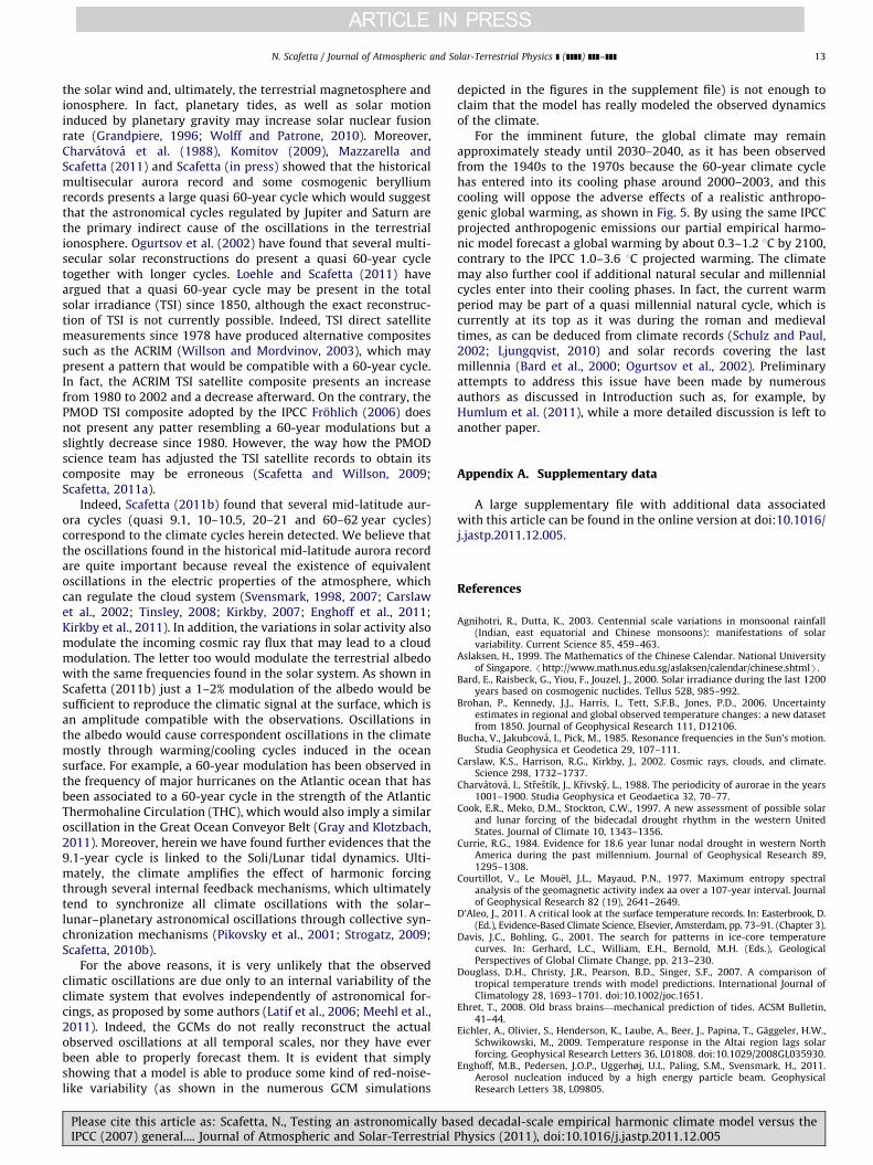
the solar wind and, ultimately, the terrestrial magnetosphere andionosphere. In fact, planetary tides, as well as solar motioninduced by planetary gravity may increase solar nuclear fusionrate (Grandpiere, 1996; Wolff and Patrone, 2010). Moreover,Charvatova et al. (1988), Komitov (2009), Mazzarella andScafetta (2011) and Scafetta (in press) showed that the historicalmultisecular aurora record and some cosmogenic berylliumrecords presents a large quasi 60-year cycle which would suggestthat the astronomical cycles regulated by Jupiter and Saturn arethe primary indirect cause of the oscillations in the terrestrialionosphere. Ogurtsov et al. (2002) have found that several multi-secular solar reconstructions do present a quasi 60-year cycletogether with longer cycles. Loehle and Scafetta (2011) haveargued that a quasi 60-year cycle may be present in the totalsolar irradiance (TSI) since 1850, although the exact reconstruc-tion of TSI is not currently possible. Indeed, TSI direct satellitemeasurements since 1978 have produced alternative compositessuch as the ACRIM (Willson and Mordvinov, 2003), which maypresent a pattern that would be compatible with a 60-year cycle.In fact, the ACRIM TSI satellite composite presents an increasefrom 1980 to 2002 and a decrease afterward. On the contrary, thePMOD TSI composite adopted by the IPCC Frohlich (2006) doesnot present any patter resembling a 60-year modulations but aslightly decrease since 1980. However, the way how the PMODscience team has adjusted the TSI satellite records to obtain itscomposite may be erroneous (Scafetta and Willson, 2009;Scafetta, 2011a).

Indeed, Scafetta (2011b) found that several mid-latitude aur-ora cycles (quasi 9.1, 10–10.5, 20–21 and 60–62 year cycles)correspond to the climate cycles herein detected. We believe thatthe oscillations found in the historical mid-latitude aurora recordare quite important because reveal the existence of equivalentoscillations in the electric properties of the atmosphere, whichcan regulate the cloud system (Svensmark, 1998, 2007; Carslawet al., 2002; Tinsley, 2008; Kirkby, 2007; Enghoff et al., 2011;Kirkby et al., 2011). In addition, the variations in solar activity alsomodulate the incoming cosmic ray flux that may lead to a cloudmodulation. The letter too would modulate the terrestrial albedowith the same frequencies found in the solar system. As shown inScafetta (2011b) just a 1–2% modulation of the albedo would besufficient to reproduce the climatic signal at the surface, which isan amplitude compatible with the observations. Oscillations inthe albedo would cause correspondent oscillations in the climatemostly through warming/cooling cycles induced in the oceansurface. For example, a 60-year modulation has been observed inthe frequency of major hurricanes on the Atlantic ocean that hasbeen associated to a 60-year cycle in the strength of the AtlanticThermohaline Circulation (THC), which would also imply a similaroscillation in the Great Ocean Conveyor Belt (Gray and Klotzbach,2011). Moreover, herein we have found further evidences that the9.1-year cycle is linked to the Soli/Lunar tidal dynamics. Ulti-mately, the climate amplifies the effect of harmonic forcingthrough several internal feedback mechanisms, which ultimatelytend to synchronize all climate oscillations with the solar–lunar–planetary astronomical oscillations through collective syn-chronization mechanisms (Pikovsky et al., 2001; Strogatz, 2009;Scafetta, 2010b).

For the above reasons, it is very unlikely that the observedclimatic oscillations are due only to an internal variability of theclimate system that evolves independently of astronomical for-cings, as proposed by some authors (Latif et al., 2006; Meehl et al.,2011). Indeed, the GCMs do not really reconstruct the actualobserved oscillations at all temporal scales, nor they have everbeen able to properly forecast them. It is evident that simplyshowing that a model is able to produce some kind of red-noise-like variability (as shown in the numerous GCM simulations

depicted in the figures in the supplement file) is not enough toclaim that the model has really modeled the observed dynamicsof the climate.

For the imminent future, the global climate may remainapproximately steady until 2030–2040, as it has been observedfrom the 1940s to the 1970s because the 60-year climate cyclehas entered into its cooling phase around 2000–2003, and thiscooling will oppose the adverse effects of a realistic anthropo-genic global warming, as shown in Fig. 5. By using the same IPCCprojected anthropogenic emissions our partial empirical harmo-nic model forecast a global warming by about 0.3–1.2 1C by 2100,contrary to the IPCC 1.0–3.6 1C projected warming. The climatemay also further cool if additional natural secular and millennialcycles enter into their cooling phases. In fact, the current warmperiod may be part of a quasi millennial natural cycle, which iscurrently at its top as it was during the roman and medievaltimes, as can be deduced from climate records (Schulz and Paul,2002; Ljungqvist, 2010) and solar records covering the lastmillennia (Bard et al., 2000; Ogurtsov et al., 2002). Preliminaryattempts to address this issue have been made by numerousauthors as discussed in Introduction such as, for example, byHumlum et al. (2011), while a more detailed discussion is left toanother paper.

Appendix A. Supplementary data

A large supplementary file with additional data associatedwith this article can be found in the online version at doi:10.1016/j.jastp.2011.12.005.

References

Agnihotri, R., Dutta, K., 2003. Centennial scale variations in monsoonal rainfall(Indian, east equatorial and Chinese monsoons): manifestations of solarvariability. Current Science 85, 459–463.

Aslaksen, H., 1999. The Mathematics of the Chinese Calendar. National Universityof Singapore. /http://www.math.nus.edu.sg/aslaksen/calendar/chinese.shtmlS.

Bard, E., Raisbeck, G., Yiou, F., Jouzel, J., 2000. Solar irradiance during the last 1200years based on cosmogenic nuclides. Tellus 52B, 985–992.

Brohan, P., Kennedy, J.J., Harris, I., Tett, S.F.B., Jones, P.D., 2006. Uncertaintyestimates in regional and global observed temperature changes: a new datasetfrom 1850. Journal of Geophysical Research 111, D12106.

Bucha, V., Jakubcova, I., Pick, M., 1985. Resonance frequencies in the Sun’s motion.Studia Geophysica et Geodetica 29, 107–111.

Carslaw, K.S., Harrison, R.G., Kirkby, J., 2002. Cosmic rays, clouds, and climate.Science 298, 1732–1737.

Charvatova, I., Strestık, J., Krivsky, L., 1988. The periodicity of aurorae in the years1001–1900. Studia Geophysica et Geodaetica 32, 70–77.

Cook, E.R., Meko, D.M., Stockton, C.W., 1997. A new assessment of possible solarand lunar forcing of the bidecadal drought rhythm in the western UnitedStates. Journal of Climate 10, 1343–1356.

Currie, R.G., 1984. Evidence for 18.6 year lunar nodal drought in western NorthAmerica during the past millennium. Journal of Geophysical Research 89,1295–1308.

Courtillot, V., Le Mouel, J.L., Mayaud, P.N., 1977. Maximum entropy spectralanalysis of the geomagnetic activity index aa over a 107-year interval. Journalof Geophysical Research 82 (19), 2641–2649.

D’Aleo, J., 2011. A critical look at the surface temperature records. In: Easterbrook, D.(Ed.), Evidence-Based Climate Science, Elsevier, Amsterdam, pp. 73–91. (Chapter 3).

Davis, J.C., Bohling, G., 2001. The search for patterns in ice-core temperaturecurves. In: Gerhard, L.C., William, E.H., Bernold, M.H. (Eds.), GeologicalPerspectives of Global Climate Change, pp. 213–230.

Douglass, D.H., Christy, J.R., Pearson, B.D., Singer, S.F., 2007. A comparison oftropical temperature trends with model predictions. International Journal ofClimatology 28, 1693–1701. doi:10.1002/joc.1651.

Ehret, T., 2008. Old brass brains—mechanical prediction of tides. ACSM Bulletin,41–44.

Eichler, A., Olivier, S., Henderson, K., Laube, A., Beer, J., Papina, T., Gaggeler, H.W.,Schwikowski, M., 2009. Temperature response in the Altai region lags solarforcing. Geophysical Research Letters 36, L01808. doi:10.1029/2008GL035930.

Enghoff, M.B., Pedersen, J.O.P., Uggerhøj, U.I., Paling, S.M., Svensmark, H., 2011.Aerosol nucleation induced by a high energy particle beam. GeophysicalResearch Letters 38, L09805.

N. Scafetta / Journal of Atmospheric and Solar-Terrestrial Physics ] (]]]]) ]]]–]]] 13

Please cite this article as: Scafetta, N., Testing an astronomically based decadal-scale empirical harmonic climate model versus theIPCC (2007) general.... Journal of Atmospheric and Solar-Terrestrial Physics (2011), doi:10.1016/j.jastp.2011.12.005

Frohlich, C., 2006. Solar irradiance variability since 1978: revision of the PMODcomposite during solar cycle 21. Space Science Reviews 125, 53–65.

Grandpiere, A., 1996. On the origin of the solar cycle periodicity. Astrophysics andSpace Science 243, 393–400.

Gray, W.M., Klotzbach, P.J., 2011. Have increases in CO2 contributed to the recent largeupswing in Atlantic basin major hurricanes since 1995?. In: Easterbrook, D. (Ed.),Evidence-Based Climate Science, Elsevier, Amsterdam, pp. 223–249. (Chapter 9).

Hansen, J., et al., 2007. Climate simulations for 1880–2003 with GISS modelE.Climate Dynamics 29, 661–696.

Hoyt, D.V., Schatten, K.H., 1997. The Role of the Sun in the Climate Change. OxfordUniv. Press, New York.

Humlum, O., Solheim, J.-K., Stordahl, K., 2011. Identifying natural contributions tolate Holocene climate change. Global and Planetary Change 79, 145–156.

IPCC, 2007. In: Solomon, S., et al. (Eds.). Climate Change 2007: The Physical ScienceBasis. Contribution of Working Group I to the Fourth Assessment Report of theIntergovernmental Panel on Climate Change. Cambridge University Press,Cambridge.

Iyengar, R.N., 2009. Monsoon rainfall cycles as depicted in ancient Sanskrit texts.Current Science 97, 444–447.

Jevrejeva, S., Moore, J.C., Grinsted, A., Woodworth, P.L., 2008. Recent global sealevel acceleration started over 200 years ago? Geophysical Research Letters 35,L08715.

Kaufmann, R.K., Kauppi, H., Mann, M.L., Stock, J.H., 2011. Reconciling anthropo-genic climate change with observed temperature 1998–2008. PNAS 108,11790–11793. doi:10.1073/pnas.1102467108.

Kennedy, J.J., Rayner, N.A., Smith, R.O., Saunby, M., Parker, D.E., 2011. Reassessingbiases and other uncertainties in sea-surface temperature observations since1850: biases and homogenisation. Journal of Geophysical Research 116,D14103–D14104.

Kirkby, J., 2007. Cosmic rays and climate. Surveys in Geophysics 28, 333–375.Kirkby, J., et al., 2011. Role of sulphuric acid, ammonia and galactic cosmic rays in

atmospheric aerosol nucleation. Nature 476, 429–433.Klyashtorin, L.B., Borisov, V., Lyubushin, A., 2009. Cyclic changes of climate and

major commercial stocks of the Barents Sea. Marine Biology Research 5, 4–17.Komitov, B., 2009. The Sun-climate relationship II: the cosmogenic beryllium and

the middle latitude aurora. Bulgarian Astronomical Journal 12, 75–90.Knudsen, M.F., Seidenkrantz, M.-S., Jacobsen, B.H., Kuijpers, A., 2011. Tracking the

Atlantic multidecadal oscillation through the last 8,000 years. Nature Com-munications 2, 178.

Latif, M., Collins, M., Pohlmann, H., Keenlyside, N., 2006. A review of predictabilitystudies of atlantic sector climate on decadal time scales. Journal of Climate 19,5971–5987.

Le Mouel, J.-L., Courtillot, V., Blanter, E., Shnirman, M., 2008. Evidence for a solarsignature in 20th-century temperature data from the USA and Europe.Geoscience 340, 421–430.

Ljungqvist, F.C., 2010. A new reconstruction of temperature variability in theextra-tropical Northern Hemisphere during the last two millennia. Geogra-fiska Annaler Series A 92, 339–351.

Lindzen, R.S., Choi, Y.-S., 2011. On the observational determination of climatesensitivity and its implications. Asia-Pacific Journal of Atmospheric Sciences47 (4), 377–390.

Liu, Y., Cai, Q.F., Song, H.M., ZhiSheng, A.N., Linderholm, H.W., 2011. Amplitudes,rates, periodicities and causes of temperature variations in the past 2485 yearsand future trends over the central-eastern Tibetan Plateau. Chinese ScienceBulletin 56, 2986–2994.

Loehle, C., Scafetta, N., 2011. Climate change attribution using empirical decom-position of climatic data. The Open Atmospheric Science Journal 5, 74–86.

Lockwood, M., 2008. Analysis of the contributions to global mean air surfacetemperature rise. Proceedings of the Royal Society A 464, 1–17.

Mazzarella, A., Scafetta, N., 2011. Evidences for a quasi 60-year North AtlanticOscillation since 1700 and its meaning for global climate change. Theoreticaland Applied Climatology. doi:10.1007/s00704-011-0499-4.

McKitrick, R., Michaels, P., 2007. Quantifying the influence of anthropogenicsurface processes and inhomogeneities on gridded global climate data. Journalof Geophysical Research 112, D24S09.

McKitrick, R., 2010. Atmospheric circulations do not explain the temperature-industrialization correlation. Statistics, Politics and Policy 1, 1.

Meehl, G.A., Arblaster, J.M., Fasullo, J.T., Hu, A., Trenberth, K.E., 2011. Model-basedevidence of deep-ocean heat uptake during surface-temperature hiatusperiods. Nature Climate Change 1, 360–364.

Ogurtsov, M.G., Nagovitsyn, Y.A., Kocharov, G.E., Jungner, H., 2002. Long-periodcycles of the Sun’s activity recorded in direct solar data and proxies. SolarPhysics 211, 371–394.

Patterson, R.T., Prokoph, A., Chang, A., 2004. Late Holocene sedimentary responseto solar and cosmic ray activity influenced climate variability in the NE Pacific.Sedimentary Geology 172, 67–84.

Pikovsky, A., Rosemblum, M., Kurths, J., 2001. Synchronization: A UniversalConcept in Nonlinear Sciences. Cambridge University Press.

Press, W.H., Teukolsky, S.A., Vetterling, W.T., Flannery, B.P., 2007. NumericalRecipes, 3rd ed. Cambridge University Press.

Scafetta, N., West, B.J., 2007. Phenomenological reconstructions of the solarsignature in the Northern Hemisphere surface temperature records since1600. Journal of Geophysical Research 112, D24S03.

Scafetta, N., 2009. Empirical analysis of the solar contribution to global mean airsurface temperature change. Journal of Atmospheric and Solar-TerrestrialPhysics 71, 1916–1923.

Scafetta, N., Willson, R.C., 2009. ACRIM-gap and TSI trend issue resolved using asurface magnetic flux TSI proxy model. Geophysical Research Letters 36,L05701.

Scafetta, N., 2010a. Climate change and its causes: a discussion about some keyissues. La Chimica e l’Industria 1, 70–75. (The English translation is publishedby Science and Public Policy Institute. http://scienceandpublicpolicy.org/originals/climate_change_causes.html).

Scafetta, N., 2010b. Empirical evidence for a celestial origin of the climateoscillations and its implications. Journal of Atmospheric and Solar-TerrestrialPhysics 72, 951–970.

Scafetta, N., 2011a. Total solar irradiance satellite composites and their phenom-enological effect on climate. In: Easterbrook, D. (Ed.), Evidence-Based ClimateScience, Elsevier, Amsterdam, pp. 289–316. (Chapter 12).

Scafetta, N., 2011b A shared frequency set between the historical mid-latitudeaurora records and the global surface temperature. Journal of Atmospheric andSolar-Terrestrial Physics 74, 145–163. doi:10.1016/j.jastp.2011.10.013.

Schulz, M., Paul, A., 2002. Holocene climate variability on centennial-to-millennialtime scales. 1. Climate records from the North-Atlantic Realm. In: Wefer, G.,Berger, W., Behre, K.-E., Jansen, E. (Eds.), Climate Development and History ofthe North Atlantic Realm. , Springer-Verlag, Berlin, Heidelberg, pp. 41–54.

Shaviv, N.J., 2008. Using the Oceans as a calorimeter to quantify the solar radiativeforcing. Journal of Geophysical Research 113, A11101. doi:10.1029/2007JA012989.

Singer, S.F., 2011. Lack of consistency between modeled and observed temperaturetrends. Energy & Environment 22 (4), 375–406.

Sinha, A., et al., 2005. Variability of southwest indian summer monsoon precipita-tion during the Bølling–Allerød. Geology 33, 813–816.

Sidorenkov, N., 2005. Long-term changes in the variance of the earth orientationparameters and of the excitation functions. In: Proceedings of the ‘‘JourneesSyst�emes de Reference Spatio-Temporels 2005’’ Warsaw, 19–21 September2005.

Soon, W., 2009. Solar Arctic-mediated climate variation on multidecadal tocentennial timescales: empirical evidence, mechanistic explanation, andtestable consequences. Physical Geography 30, 144–184.

Soon, W., Dutta, K., Legates, D.R., Velasco, V., Zhang, W., 2011. Variation in surfaceair temperature of China during the 20th century. Journal of Atmospheric andSolar-Terrestrial Physics 73 (16), 2331–2344.

Spencer, R.W., Braswell, W.D., 2011. On the misdiagnosis of surface temperaturefeedbacks from variations in earth’s radiant energy balance. Remote Sensing 3,1603–1613.

Sonnemann, G., 1998. Comment on ‘‘Does the correlation between solar cyclelength and Northern Hemisphere and temperatures rule out any significantglobal warming from greenhouse gases?’’ By Peter Laut and JasperGrundmann. Journal of Atmospheric and Solar Terrestrial Physics 60,1625–1630.

Stockton, C.W., Mitchell, J.M., Meko, D.M., 1983. A reappraisal of the 22-yeardrought cycle. In: McCormac, B.M. (Ed.), Solar-Terrestrial Influences onWeather and Climate. , Colorado Associated University Press, pp. 507–515.

Strogatz, S.H., 2009. Exploring complex networks. Nature 410, 268–276.Svensmark, H., 1998. Influence of cosmic rays on Earth’s climate. Physical Review

Letters 81 (22), 5027–5030.Svensmark, H., 2007. Cosmoclimatology: a new theory emerges. Astronomy &

Geophysics 48, 1.18–1.24.Temple, R.K.G., 1998. The Sirius Mystery. Destiny Books. In ‘‘Appendix III: Why

Sixty Years?’’ /http://www.bibliotecapleyades.net/universo/siriusmystery/siriusmystery.htmS.

Thejll, P., Lassen, K., 2000. Solar forcing of the Northern hemisphere land airtemperature: new data. Journal of Atmospheric and Solar-Terrestrial Physics62, 1207–1213.

Thompson, D.W.J., Wallace, J.M., Jones, P.D., Kennedy, J.J., 2009. Identifyingsignatures of natural climate variability in time series of global-mean surfacetemperature: methodology and insights. Journal of Climate 22, 6120–6141.

Thomson, W., 1881. The tide gauge, tidal harmonic analyzer, and tide predictor.Proceedings of the Institution of Civil Engineers 65, 3–24. (Lord Kelvin).

Tinsley, B.A., 2008. The global atmospheric electric circuit and its effects on cloudmicrophysics. Reports on Progress in Physics 71, 066801.

Tisdale, B., 2010. GISS Deletes Arctic and Southern Ocean Sea Surface TemperatureData. /http://wattsupwiththat.com/2010/05/31/giss-deletes-arctic-and-southern-ocean-sea-surface-temperature-data/S.

Weihong, Q., Bo, L., 2010. Periodic oscillations in millennial global-mean tem-perature and their causes. Chinese Science Bulletin 35, 4052–4057.

Willson, R.C., Mordvinov, A.V., 2003. Secular total solar irradiance trend duringsolar cycles 21–23. Geophysical Research Letters 30, 1199–1282.

Wolff, C.L., Patrone, P.N., 2010. A new way that planets can affect the sun. SolarPhysics 266, 227–246.

Yadava, M.G., Ramesh, R., 2007. Significant longer-term periodicities in the proxyrecord of the Indian monsoon rainfall. New Astronomy 12, 544–555.

Yu, Z., Chang, S., Kumazawa, M., Furumoto, M., Yamamoto, A., 1983. Presence ofperiodicity in meteorite falls. Memoirs of National Institute of Polar Research30, 362–366. (Special issue).

N. Scafetta / Journal of Atmospheric and Solar-Terrestrial Physics ] (]]]]) ]]]–]]]14

Please cite this article as: Scafetta, N., Testing an astronomically based decadal-scale empirical harmonic climate model versus theIPCC (2007) general.... Journal of Atmospheric and Solar-Terrestrial Physics (2011), doi:10.1016/j.jastp.2011.12.005

J. of Atmospheric and Solar-Terrestrial Physics, 2011.

Supplement file for

“Testing an astronomically-based decadal-scale empirical harmonic climate model vs. the IPCC (2007) general circulation climate models”

Nicola Scafetta

Section 1: page 2

Power spectrum comparison: HadCRUT3, GISSTEM/250, GHCN-Mv3

Section 2: page 3-28

Testing the IPCC climate models against the the 20 and 60-year global surface temperature cycles

Section 3: page 29-31

Testing the Maximum Entropy Method

Section 4: page 32-33

IPCC 2007 mean anthropogenic net warming trend from 1970 to 2050

Section 5: page 34

Overestimation of the GISS ModelE reconstruction of the volcano signature and comparison with the empirical climate of the volcano signature

Section 6: page 35-36

The 9-year cycle of Lunar and Solar eclipses at the equinoxes in 1997 and in 2006, respectively

Section 7: page 37

Preliminary attempts to interpret the warming since 1850 as partially due to multisecular and millennial cycles

Figure S1. [A] The figure shows a comparison between the three available global surface temperature signals: HadCRUT3, GISSTEM with 250km smooth and NOAA GHCN-Mv3 since 1880. The power spectra records look similar. The detected frequency peaks match those found for the speed of the Sun relative to the solar system barycenter: look at Table 2 in Scafetta (2011b). [B] The power spectra are evaluated with the MEM with 790 poles (top) (see Section 3 for explanation) and with the Lomb periodogram (bottom). The power spectra look similar and present similar main peaks. These include the four peaks discussed in the text, as shown in the figure. The 20 and 60-year cycles are the major one, the decadal cycle is also large because made of two cycles. (The linear upward trending is detrended before the PS analysis)

60-6220-219.1

10.214.2

7.56.35.2

Data from : http://climexp.knmi.nl/selectfield_obs.cgi?someone@somewhere

Section 1: page 2.Power spectrum comparison:HadCRUT3, GISSTEM/250, GHCN-Mv3

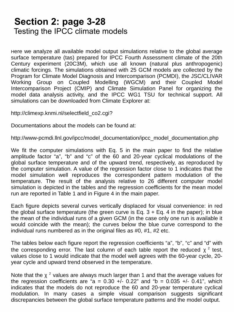
Section 2: page 3-28Testing the IPCC climate models

Here we analyze all available model output simulations relative to the global average surface temperature (tas) prepared for IPCC Fourth Assessment climate of the 20th Century experiment (20C3M), which use all known (natural plus anthropogenic) climatic forcings. The simulations obtained with 25 GCM models are collected by the Program for Climate Model Diagnosis and Intercomparison (PCMDI), the JSC/CLIVAR Working Group on Coupled Modelling (WGCM) and their Coupled Model Intercomparison Project (CMIP) and Climate Simulation Panel for organizing the model data analysis activity, and the IPCC WG1 TSU for technical support. All simulations can be downloaded from Climate Explorer at:

http://climexp.knmi.nl/selectfield_co2.cgi?

Documentations about the models can be found at:

http://www-pcmdi.llnl.gov/ipcc/model_documentation/ipcc_model_documentation.php

We fit the computer simulations with Eq. 5 in the main paper to find the relative amplitude factor “a”, “b” and “c” of the 60 and 20-year cyclical modulations of the global surface temperature and of the upward trend, respectively, as reproduced by the computer simulation. A value of the regression factor close to 1 indicates that the model simulation well reproduces the correspondent pattern modulation of the temperature. The result of the analysis relative to 26 different computer model simulation is depicted in the tables and the regression coefficients for the mean model run are reported in Table 1 and in Figure 4 in the main paper.

Each figure depicts several curves vertically displaced for visual convenience: in red the global surface temperature (the green curve is Eq. 3 + Eq. 4 in the paper); in blue the mean of the individual runs of a given GCM (in the case only one run is available it would coincide with the mean); the curves below the blue curve correspond to the individual runs numbered as in the original files as #0, #1, #2 etc.

The tables below each figure report the regression coefficients “a”, “b”, “c” and “d” with the corresponding error. The last column of each table report the reduced χ 2 test, values close to 1 would indicate that the model well agrees with the 60-year cycle, 20-year cycle and upward trend observed in the temperature.

Note that the χ 2 values are always much larger than 1 and that the average values for the regression coefficients are “a = 0.30 +/- 0.22” and “b = 0.035 +/- 0.41”, which indicates that the models do not reproduce the 60 and 20-year temperature cyclical modulation. In many cases a simple visual comparison suggests significant discrepancies between the global surface temperature patterns and the model output.

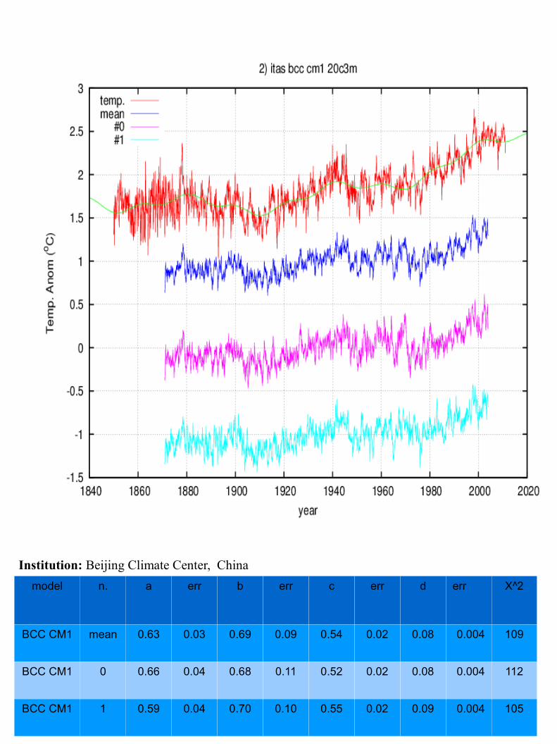
model n. a err b err c err d err X^2

BCC CM1 mean 0.63 0.03 0.69 0.09 0.54 0.02 0.08 0.004 109

BCC CM1 0 0.66 0.04 0.68 0.11 0.52 0.02 0.08 0.004 112

BCC CM1 1 0.59 0.04 0.70 0.10 0.55 0.02 0.09 0.004 105

Institution: Beijing Climate Center, China

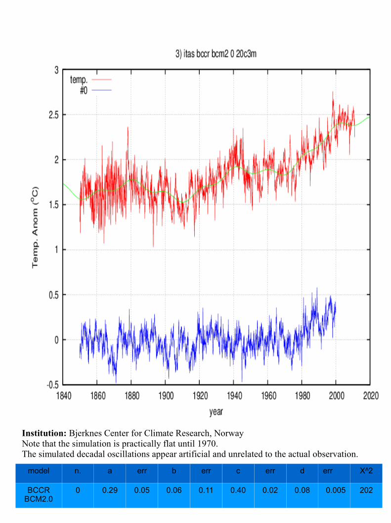
model n. a err b err c err d err X^2

BCCR BCM2.0

0 0.29 0.05 0.06 0.11 0.40 0.02 0.08 0.005 202

Institution: Bjerknes Center for Climate Research, NorwayNote that the simulation is practically flat until 1970.The simulated decadal oscillations appear artificial and unrelated to the actual observation.

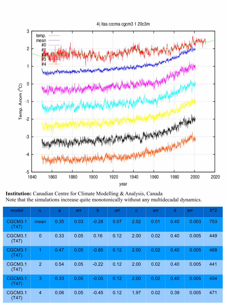
model n. a err b err c err d err X^2

CGCM3.1 (T47)

mean 0.35 0.03 -0.28 0.07 2.02 0.01 0.40 0.003 753

CGCM3.1 (T47)

0 0.33 0.05 0.16 0.12 2.00 0.02 0.40 0.005 449

CGCM3.1 (T47)

1 0.47 0.05 -0.85 0.12 2.00 0.02 0.40 0.005 468

CGCM3.1 (T47)

2 0.54 0.05 -0.22 0.12 2.00 0.02 0.40 0.005 441

CGCM3.1 (T47)

3 0.33 0.05 -0.05 0.12 2.00 0.02 0.40 0.005 454

CGCM3.1 (T47)

4 0.06 0.05 -0.45 0.12 1.97 0.02 0.39 0.005 471

Institution: Canadian Centre for Climate Modelling & Analysis, CanadaNote that the simulations increase quite monotonically without any multidecadal dynamics.

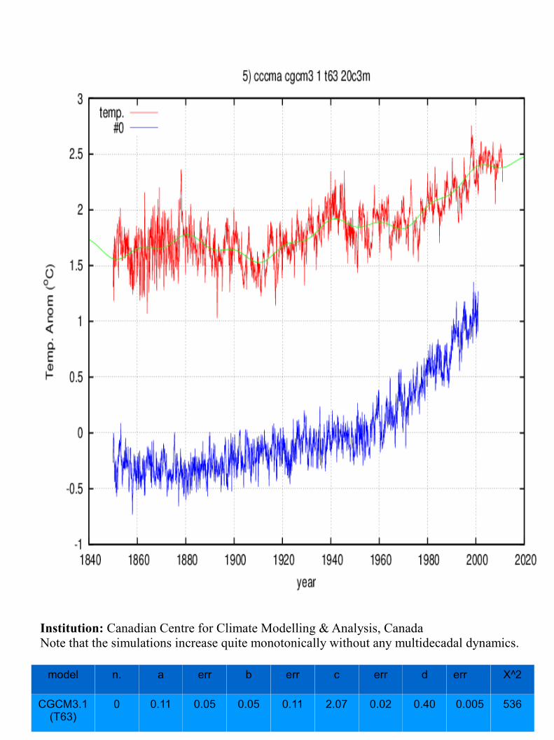
model n. a err b err c err d err X^2

CGCM3.1 (T63)

0 0.11 0.05 0.05 0.11 2.07 0.02 0.40 0.005 536

Institution: Canadian Centre for Climate Modelling & Analysis, CanadaNote that the simulations increase quite monotonically without any multidecadal dynamics.

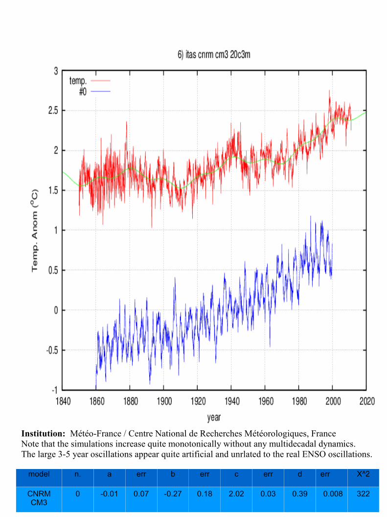
model n. a err b err c err d err X^2

CNRM CM3

0 -0.01 0.07 -0.27 0.18 2.02 0.03 0.39 0.008 322

Institution: Météo-France / Centre National de Recherches Météorologiques, FranceNote that the simulations increase quite monotonically without any multidecadal dynamics. The large 3-5 year oscillations appear quite artificial and unrlated to the real ENSO oscillations.

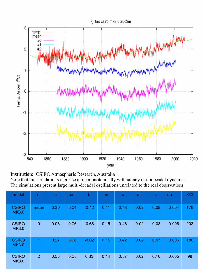
model n. a err b err c err d err X^2

CSIRO MK3.0

mean 0.30 0.04 -0.12 0.11 0.48 0.02 0.08 0.004 176

CSIRO MK3.0

0 0.06 0.06 -0.68 0.15 0.46 0.02 0.08 0.006 203

CSIRO MK3.0

1 0.27 0.06 -0.02 0.15 0.42 0.02 0.07 0.006 186

CSIRO MK3.0

2 0.58 0.05 0.33 0.14 0.57 0.02 0.10 0.005 98

Institution: CSIRO Atmospheric Research, AustraliaNote that the simulations increase quite monotonically without any multidecadal dynamics.The simulations present large multi-decadal oscillations unrelated to the real observations

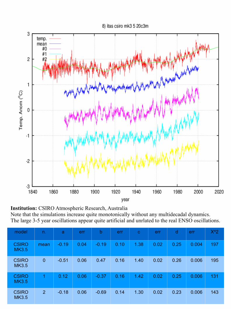
model n. a err b err c err d err X^2

CSIRO MK3.5

mean -0.19 0.04 -0.19 0.10 1.38 0.02 0.25 0.004 197

CSIRO MK3.5

0 -0.51 0.06 0.47 0.16 1.40 0.02 0.26 0.006 195

CSIRO MK3.5

1 0.12 0.06 -0.37 0.16 1.42 0.02 0.25 0.006 131

CSIRO MK3.5

2 -0.18 0.06 -0.69 0.14 1.30 0.02 0.23 0.006 143

Institution: CSIRO Atmospheric Research, AustraliaNote that the simulations increase quite monotonically without any multidecadal dynamics. The large 3-5 year oscillations appear quite artificial and unrlated to the real ENSO oscillations.

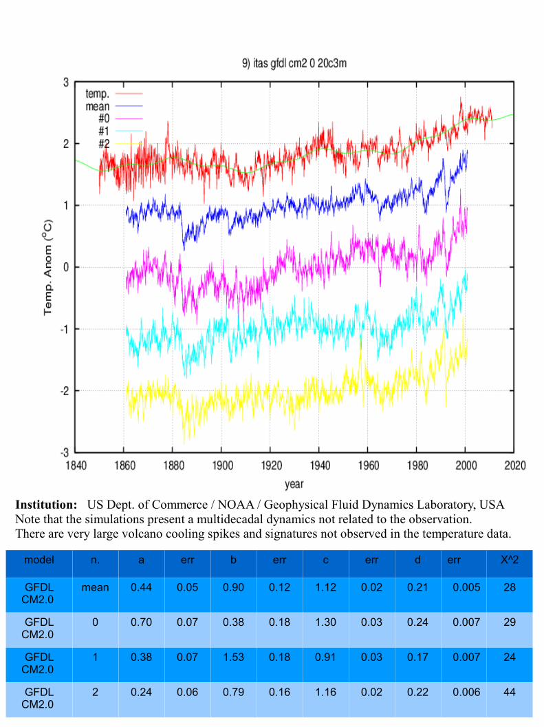
model n. a err b err c err d err X^2

GFDL CM2.0

mean 0.44 0.05 0.90 0.12 1.12 0.02 0.21 0.005 28

GFDL CM2.0

0 0.70 0.07 0.38 0.18 1.30 0.03 0.24 0.007 29

GFDL CM2.0

1 0.38 0.07 1.53 0.18 0.91 0.03 0.17 0.007 24

GFDL CM2.0

2 0.24 0.06 0.79 0.16 1.16 0.02 0.22 0.006 44

Institution: US Dept. of Commerce / NOAA / Geophysical Fluid Dynamics Laboratory, USANote that the simulations present a multidecadal dynamics not related to the observation.There are very large volcano cooling spikes and signatures not observed in the temperature data.

model n. a err b err c err d err X^2

GFDL CM2.1

mean 0.37 0.07 0.75 0.17 1.37 0.03 0.26 0.007 53

GFDL CM2.1

0 0.77 0.09 1.19 0.22 1.38 0.03 0.26 0.009 37

GFDL CM2.1

1 0.43 0.09 0.52 0.21 1.29 0.03 0.24 0.009 33

GFDL CM2.1

2 -0.10 0.10 0.53 0.25 1.45 0.04 0.28 0.010 67

Institution: US Dept. of Commerce / NOAA / Geophysical Fluid Dynamics Laboratory, USANote that the simulations present a large 3-5 year oscillations and multidecadal dynamics not related to the observation. There are very large volcano cooling spikes and signatures not observed in the temperature data.

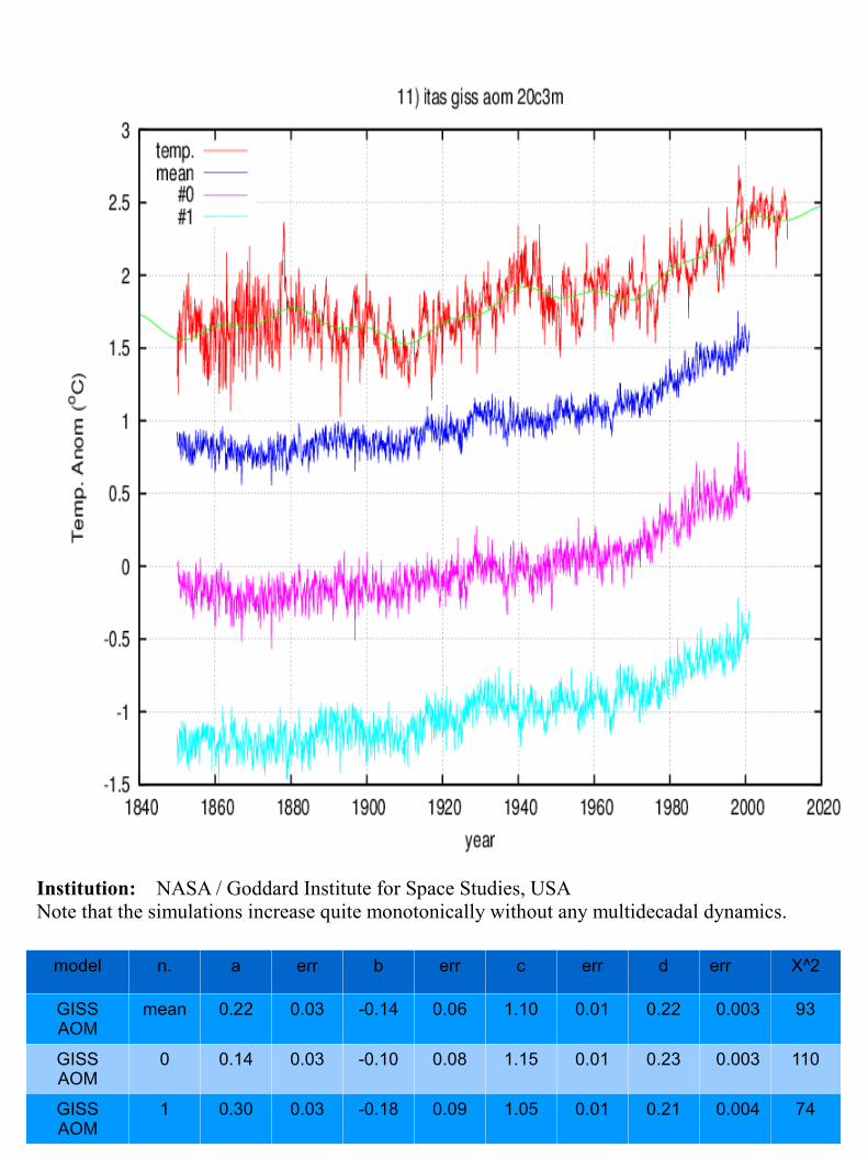
model n. a err b err c err d err X^2

GISS AOM

mean 0.22 0.03 -0.14 0.06 1.10 0.01 0.22 0.003 93

GISS AOM

0 0.14 0.03 -0.10 0.08 1.15 0.01 0.23 0.003 110

GISS AOM

1 0.30 0.03 -0.18 0.09 1.05 0.01 0.21 0.004 74

Institution: NASA / Goddard Institute for Space Studies, USANote that the simulations increase quite monotonically without any multidecadal dynamics.

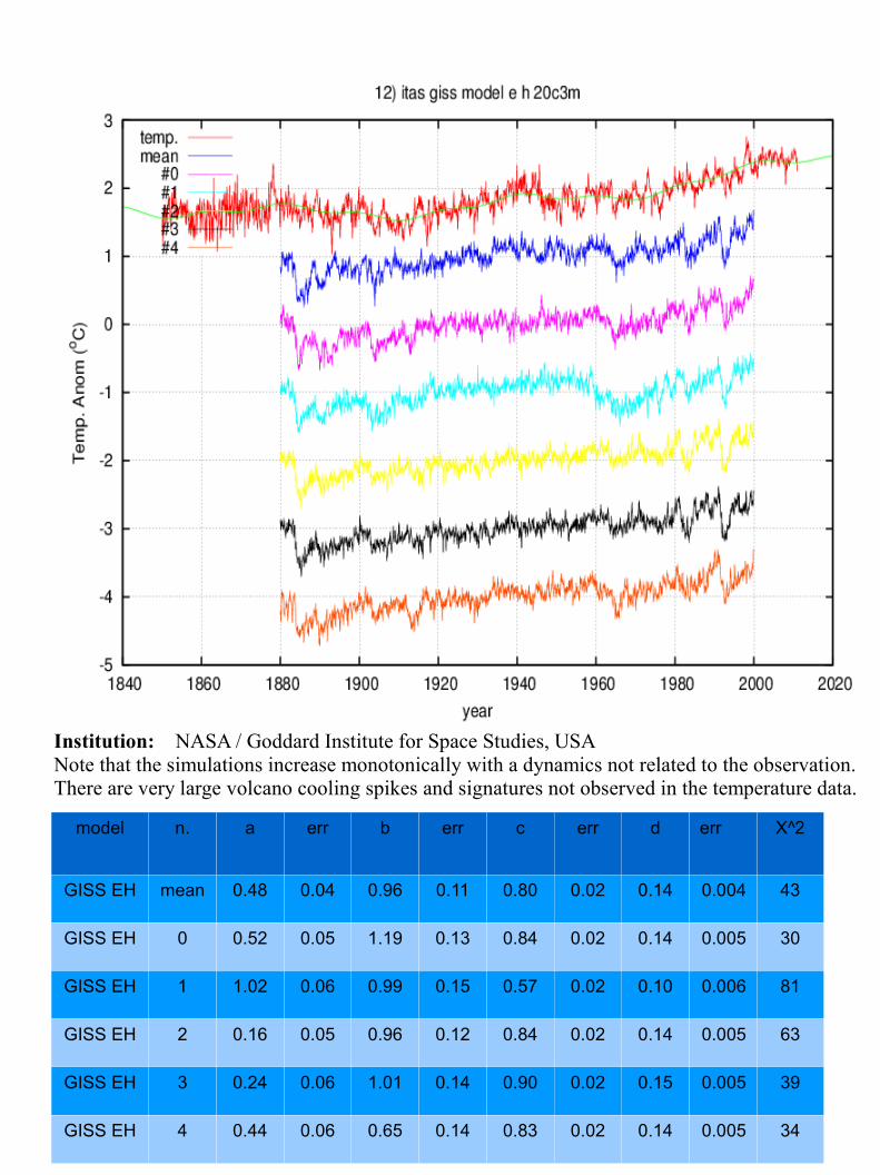
model n. a err b err c err d err X^2

GISS EH mean 0.48 0.04 0.96 0.11 0.80 0.02 0.14 0.004 43

GISS EH 0 0.52 0.05 1.19 0.13 0.84 0.02 0.14 0.005 30

GISS EH 1 1.02 0.06 0.99 0.15 0.57 0.02 0.10 0.006 81

GISS EH 2 0.16 0.05 0.96 0.12 0.84 0.02 0.14 0.005 63

GISS EH 3 0.24 0.06 1.01 0.14 0.90 0.02 0.15 0.005 39

GISS EH 4 0.44 0.06 0.65 0.14 0.83 0.02 0.14 0.005 34

Institution: NASA / Goddard Institute for Space Studies, USANote that the simulations increase monotonically with a dynamics not related to the observation.There are very large volcano cooling spikes and signatures not observed in the temperature data.

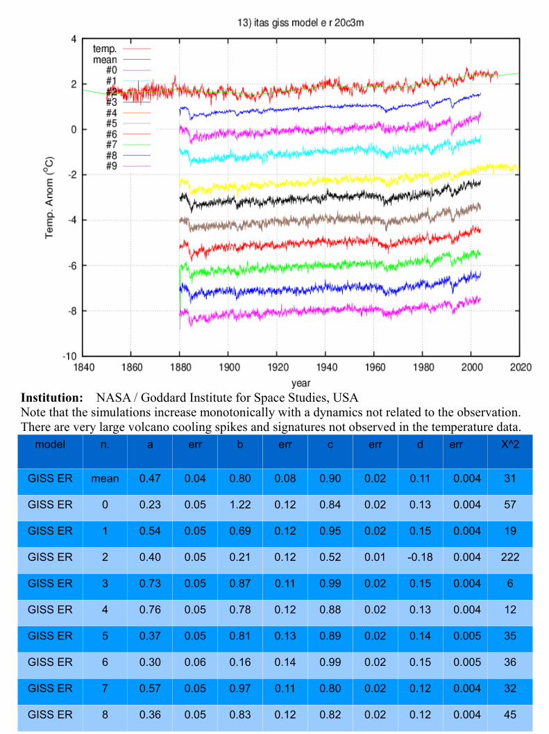
model n. a err b err c err d err X^2

GISS ER mean 0.47 0.04 0.80 0.08 0.90 0.02 0.11 0.004 31

GISS ER 0 0.23 0.05 1.22 0.12 0.84 0.02 0.13 0.004 57

GISS ER 1 0.54 0.05 0.69 0.12 0.95 0.02 0.15 0.004 19

GISS ER 2 0.40 0.05 0.21 0.12 0.52 0.01 -0.18 0.004 222

GISS ER 3 0.73 0.05 0.87 0.11 0.99 0.02 0.15 0.004 6

GISS ER 4 0.76 0.05 0.78 0.12 0.88 0.02 0.13 0.004 12

GISS ER 5 0.37 0.05 0.81 0.13 0.89 0.02 0.14 0.005 35

GISS ER 6 0.30 0.06 0.16 0.14 0.99 0.02 0.15 0.005 36

GISS ER 7 0.57 0.05 0.97 0.11 0.80 0.02 0.12 0.004 32

GISS ER 8 0.36 0.05 0.83 0.12 0.82 0.02 0.12 0.004 45

Institution: NASA / Goddard Institute for Space Studies, USANote that the simulations increase monotonically with a dynamics not related to the observation.There are very large volcano cooling spikes and signatures not observed in the temperature data.

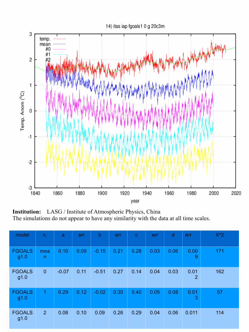
model n. a err b err c err d err X^2

FGOALS g1.0

mean

0.10 0.09 -0.15 0.21 0.28 0.03 0.06 0.009

171

FGOALS g1.0

0 -0.07 0.11 -0.51 0.27 0.14 0.04 0.03 0.012

162

FGOALS g1.0

1 0.29 0.12 -0.02 0.30 0.40 0.05 0.08 0.013

57

FGOALS g1.0

2 0.08 0.10 0.09 0.26 0.29 0.04 0.06 0.011 114

Institution: LASG / Institute of Atmospheric Physics, ChinaThe simulations do not appear to have any similarity with the data at all time scales.

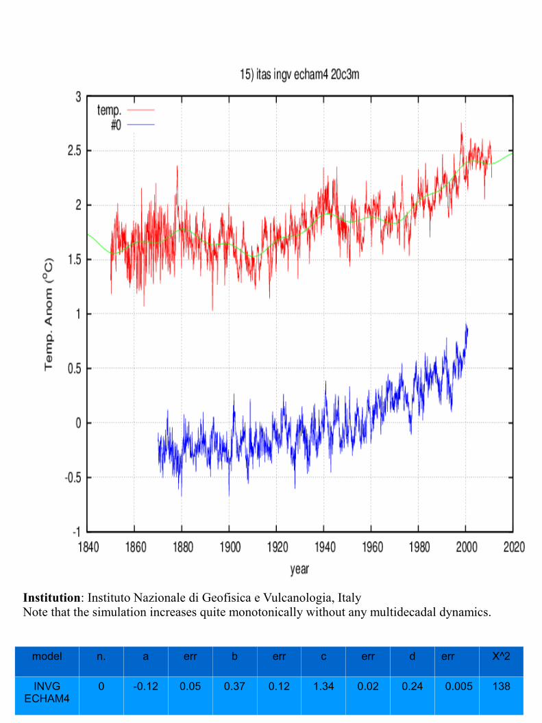
model n. a err b err c err d err X^2

INVG ECHAM4

0 -0.12 0.05 0.37 0.12 1.34 0.02 0.24 0.005 138

Institution: Instituto Nazionale di Geofisica e Vulcanologia, ItalyNote that the simulation increases quite monotonically without any multidecadal dynamics.

model n. a err b err c err d err X^2

INM CM3.0

0 0.30 0.07 0.47 0.18 1.34 0.03 0.24 0.007 54

Institution: Institute for Numerical Mathematics, RussiaNote that the simulation increases quite monotonically with a decadal and multidecadal dynamics quite unrelated to the observations.

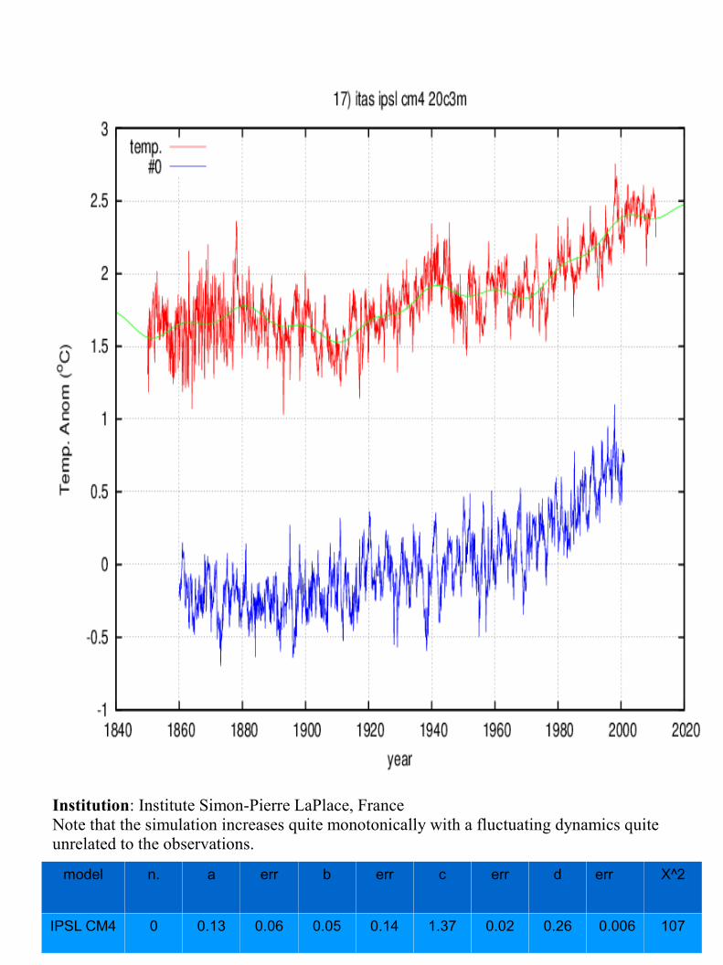
model n. a err b err c err d err X^2

IPSL CM4 0 0.13 0.06 0.05 0.14 1.37 0.02 0.26 0.006 107

Institution: Institute Simon-Pierre LaPlace, FranceNote that the simulation increases quite monotonically with a fluctuating dynamics quite unrelated to the observations.

model n. a err b err c err d err X^2

MIROC3.2 Hires

0 0.35 0.05 0.92 0.12 1.43 0.02 0.19 0.004 104

Institution: Center for Climate System Research (The University of Tokyo), JapanNote that the simulation increases quite monotonically with a fluctuating dynamics quite unrelated to the observations and large volcano cooling spikes not observed in the temperature.

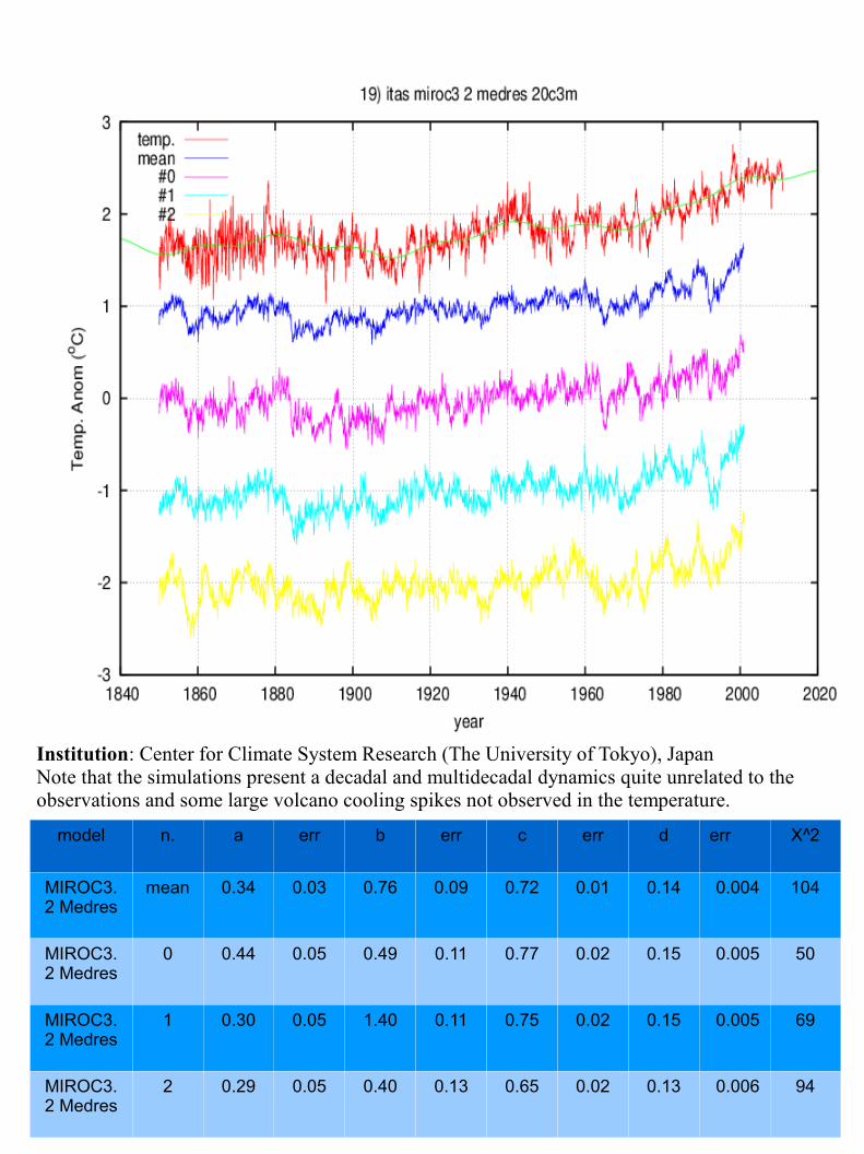
model n. a err b err c err d err X^2

MIROC3.2 Medres

mean 0.34 0.03 0.76 0.09 0.72 0.01 0.14 0.004 104

MIROC3.2 Medres

0 0.44 0.05 0.49 0.11 0.77 0.02 0.15 0.005 50

MIROC3.2 Medres

1 0.30 0.05 1.40 0.11 0.75 0.02 0.15 0.005 69

MIROC3.2 Medres

2 0.29 0.05 0.40 0.13 0.65 0.02 0.13 0.006 94

Institution: Center for Climate System Research (The University of Tokyo), JapanNote that the simulations present a decadal and multidecadal dynamics quite unrelated to the observations and some large volcano cooling spikes not observed in the temperature.

model n. a err b err c err d err X^2

ECHO G mean 0.58 0.04 0.16 0.10 0.98 0.02 0.18 0.004 26

ECHO G 0 0.66 0.07 0.87 0.16 0.94 0.03 0.18 0.006 8

ECHO G 1 0.68 0.06 -0.63 0.16 1.07 0.03 0.20 0.006 29

ECHO G 2 0.42 0.07 0.57 0.17 0.96 0.03 0.18 0.007 19

ECHO G 3 0.51 0.06 0.21 0.15 0.89 0.03 0.17 0.006 24

ECHO G 4 0.64 0.06 -0.23 0.15 1.06 0.03 0.20 0.006 22

Institution: Meteorological Institute of the University of Bonn, Meteorological Research Institute of KMA, and Model and Data group, Germany / KoreaNote that the simulations present 2-3 year large oscillations, a decadal and multidecadal dynamics and some large volcano spikes unrelated to the observations

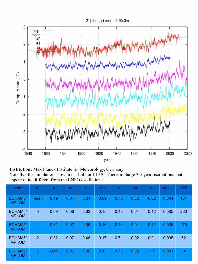
model n. a err b err c err d err X^2

ECHAM5/MPI-OM

mean 0.19 0.04 0.31 0.09 0.70 0.02 -0.02 0.004 104

ECHAM5/MPI-OM

0 0.69 0.06 0.32 0.15 0.43 0.01 -0.12 0.005 260

ECHAM5/MPI-OM

1 0.32 0.07 0.09 0.16 0.43 0.01 -0.12 0.005 279

ECHAM5/MPI-OM

2 0.32 0.07 0.46 0.17 0.71 0.02 -0.01 0.005 62

ECHAM5/MPI-OM

3 -0.09 0.07 0.30 0.17 0.78 0.03 0.15 0.007 74

Institution: Max Planck Institute for Meteorology, GermanyNote that the simulations are almost flat until 1970. There are large 3-5 year oscillations that appear quite different from the ENSO oscillations.

model n. a err b err c err d err X^2

MRI CGCM 2.3.2

mean 0.31 0.03 0.03 0.07 1.36 0.01 0.27 0.004 149

MRI CGCM 2.3.2

0 0.05 0.05 0.23 0.13 1.37 0.02 0.27 0.005 125

MRI CGCM 2.3.2

1 0.44 0.05 -0.32 0.13 1.21 0.02 0.24 0.005 58

MRI CGCM 2.3.2

2 0.46 0.05 0.34 0.13 1.54 0.02 0.31 0.005 143

MRI CGCM 2.3.2

3 0.31 0.05 -0.43 0.12 0.14 0.02 0.28 0.005 373

MRI CGCM 2.3.2

4 0.29 0.05 0.30 0.12 1.33 0.02 0.26 0.005 85

Institution: Meteorological Research Institute, JapanNote that the simulations increase quite monotonically without any multidecadal dynamics.

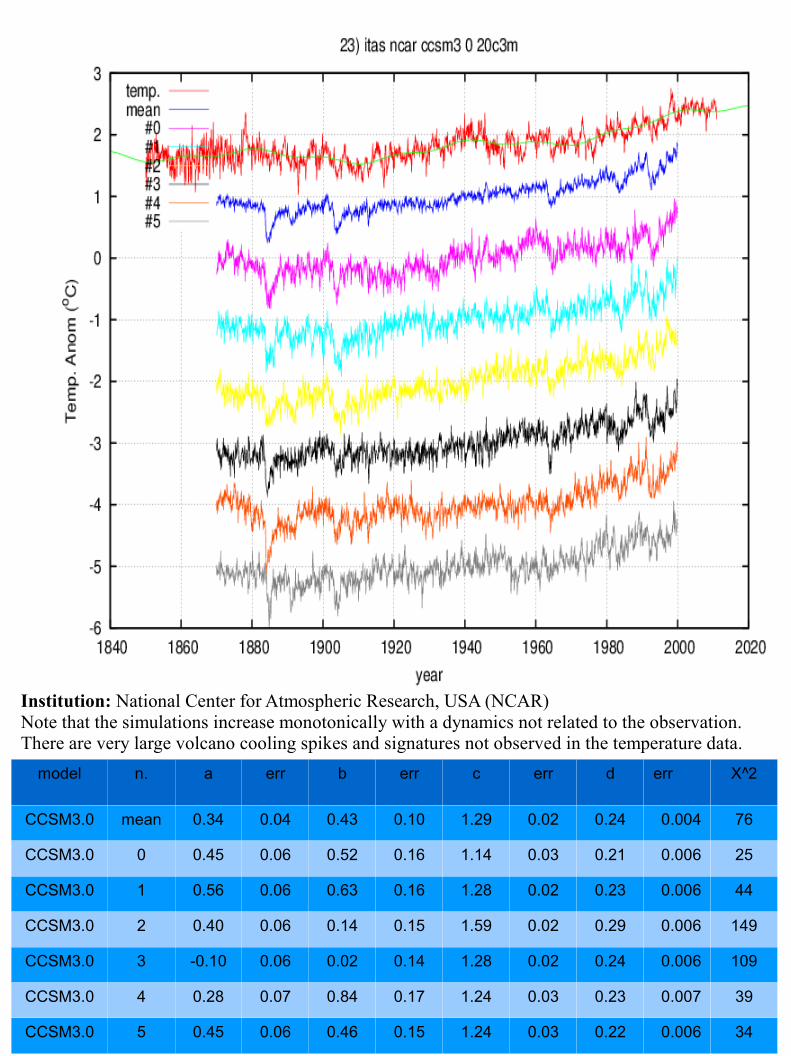
model n. a err b err c err d err X^2

CCSM3.0 mean 0.34 0.04 0.43 0.10 1.29 0.02 0.24 0.004 76

CCSM3.0 0 0.45 0.06 0.52 0.16 1.14 0.03 0.21 0.006 25

CCSM3.0 1 0.56 0.06 0.63 0.16 1.28 0.02 0.23 0.006 44

CCSM3.0 2 0.40 0.06 0.14 0.15 1.59 0.02 0.29 0.006 149

CCSM3.0 3 -0.10 0.06 0.02 0.14 1.28 0.02 0.24 0.006 109

CCSM3.0 4 0.28 0.07 0.84 0.17 1.24 0.03 0.23 0.007 39

CCSM3.0 5 0.45 0.06 0.46 0.15 1.24 0.03 0.22 0.006 34

Institution: National Center for Atmospheric Research, USA (NCAR)Note that the simulations increase monotonically with a dynamics not related to the observation.There are very large volcano cooling spikes and signatures not observed in the temperature data.

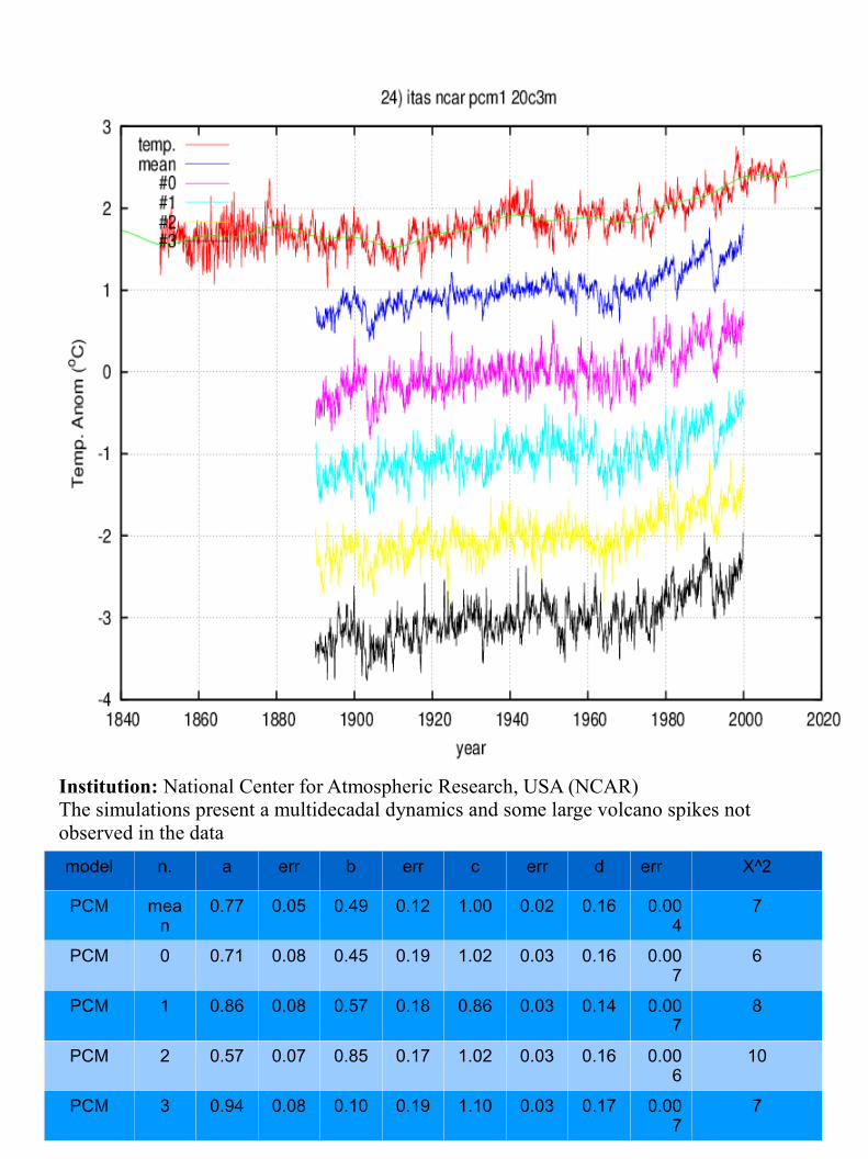
model n. a err b err c err d err X^2

PCM mean

0.77 0.05 0.49 0.12 1.00 0.02 0.16 0.004

7

PCM 0 0.71 0.08 0.45 0.19 1.02 0.03 0.16 0.007

6

PCM 1 0.86 0.08 0.57 0.18 0.86 0.03 0.14 0.007

8

PCM 2 0.57 0.07 0.85 0.17 1.02 0.03 0.16 0.006

10

PCM 3 0.94 0.08 0.10 0.19 1.10 0.03 0.17 0.007

7

Institution: National Center for Atmospheric Research, USA (NCAR)The simulations present a multidecadal dynamics and some large volcano spikes not observed in the data

model n. a err b err c err d err X^2

UKMO HADCM3

mean 0.28 0.05 0.56 0.11 0.94 0.02 0.18 0.005 42

UKMO HADCM3

0 0.13 0.06 0.75 0.15 0.90 0.03 0.18 0.006 47

UKMO HADCM3

1 0.42 0.06 0.36 0.13 0.97 0.02 0.19 0.006 25

Institution: Hadley Centre for Climate Prediction and Research / Met Office, UKNote that the simulations are almost flat until1970.

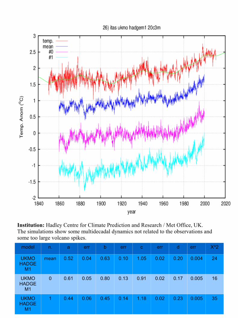
model n. a err b err c err d err X^2

UKMO HADGE

M1

mean 0.52 0.04 0.63 0.10 1.05 0.02 0.20 0.004 24

UKMO HADGE

M1

0 0.61 0.05 0.80 0.13 0.91 0.02 0.17 0.005 16

UKMO HADGE

M1

1 0.44 0.06 0.45 0.14 1.18 0.02 0.23 0.005 35

Institution: Hadley Centre for Climate Prediction and Research / Met Office, UK.The simulations show some multidecadal dynamics not related to the observations and some too large volcano spikes.

Section 3: page 29-31Testing the Maximum Entropy Method

In Figure 3 in the paper and in the previous Section 1, we have used Maximum Entropy Method (MEM) power spectrum estimates to determine that the global surface temperature record presents major cycles at about 9.1, 10-10.5, 20, 60 year periodicities. These estimates were performed in Scafetta (2010b).

MEM is a peculiar methodology whose output strongly depends on a free parameter called pole order M (Priestley, 1981; Press et al., 2004). In Scafetta (2010b) the calculations are done with a pole number M equal to half of the length N of the monthly data points since 1850. Thus, I used a value of M ≈ 1000 because N ≈ 2000.

My choice of using M ≈ 1000 may surprise some readers because in the textbooks for N = 1000 or 10000 it is usually advised to use from M = 20 to M = 50. The claim is that using a larger number of poles would produce spurious galore of peaks. Thus, a reader may seriously question my choice of using a so large value of poles, M ≈ 1000, for my analysis. So, I believe that this issue needs to be clarified for those readers who do not have a practical expertise with MEM.

First, a reader needs to realize that, as I explained in the Introduction, the frequencies that I found have been approximately found also by numerous other authors by using numerous methodologies of data analysis and also different climate records. Moreover, in Scafetta (2010b), MEM has also been applied to study the frequencies of an astronomical planetary record whose frequencies can be directly deduced from the orbits of the planets. So, the accuracy of the results of MEM could be directly evaluated. So, my estimates cannot be lightly questioned because they are supported by numerous other studies and by celestial mechanics as I also explain in the Introduction.

About the MEM pole order M, it is important to well understand its mathematical meaning and the mathematical advantage of the MEM methodology against other power spectrum techniques of analysis such as the Lomb periodogram or Fourier transforms. To address the latter issue it is important to realize that it is no true that MEM produces a spurious peak galore, while the other methods do not. All techniques produce the same numerous peaks which include a strong galore at all frequencies because all techniques attempt to give an estimate of the power associated at each frequency. The major advantage of MEM is that it produces much sharper peaks that allow a more detailed analysis of the low-frequency band of the spectrum. The MEM peaks are also higher in the presence of a small true ciclicity, and MEM also reduces the frequency leakage that may corrupt the periodogram estimates.

The maximum number of theoretically possible poles is M = N/2. This parameter measures the order of the autoregressive model used to evaluate the MEM power spectrum. Larger values of M allow the technique to detect a larger number of peaks which are always true relative to the geometry of the time series, although the smallest galore peak might not have a physical meaning. The detection of a higher density of peaks also implies that the resolution of the methodology increases with M.

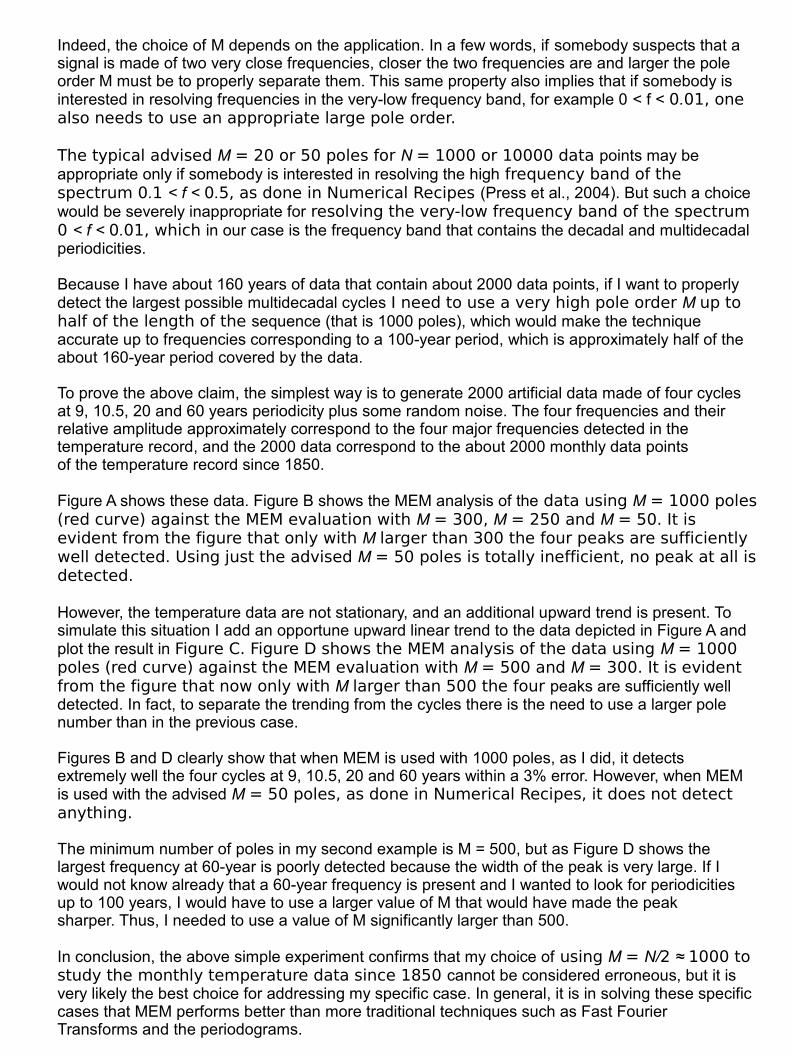
Indeed, the choice of M depends on the application. In a few words, if somebody suspects that a signal is made of two very close frequencies, closer the two frequencies are and larger the pole order M must be to properly separate them. This same property also implies that if somebody is interested in resolving frequencies in the very-low frequency band, for example 0 < f < 0.01, one also needs to use an appropriate large pole order.

The typical advised M = 20 or 50 poles for N = 1000 or 10000 data points may be appropriate only if somebody is interested in resolving the high frequency band of the spectrum 0.1 < f < 0.5, as done in Numerical Recipes (Press et al., 2004). But such a choice would be severely inappropriate for resolving the very-low frequency band of the spectrum 0 < f < 0.01, which in our case is the frequency band that contains the decadal and multidecadal periodicities.

Because I have about 160 years of data that contain about 2000 data points, if I want to properly detect the largest possible multidecadal cycles I need to use a very high pole order M up to half of the length of the sequence (that is 1000 poles), which would make the technique accurate up to frequencies corresponding to a 100-year period, which is approximately half of the about 160-year period covered by the data.

To prove the above claim, the simplest way is to generate 2000 artificial data made of four cycles at 9, 10.5, 20 and 60 years periodicity plus some random noise. The four frequencies and their relative amplitude approximately correspond to the four major frequencies detected in the temperature record, and the 2000 data correspond to the about 2000 monthly data pointsof the temperature record since 1850.

Figure A shows these data. Figure B shows the MEM analysis of the data using M = 1000 poles (red curve) against the MEM evaluation with M = 300, M = 250 and M = 50. It is evident from the figure that only with M larger than 300 the four peaks are sufficiently well detected. Using just the advised M = 50 poles is totally inefficient, no peak at all is detected.

However, the temperature data are not stationary, and an additional upward trend is present. To simulate this situation I add an opportune upward linear trend to the data depicted in Figure A and plot the result in Figure C. Figure D shows the MEM analysis of the data using M = 1000poles (red curve) against the MEM evaluation with M = 500 and M = 300. It is evident from the figure that now only with M larger than 500 the four peaks are sufficiently well detected. In fact, to separate the trending from the cycles there is the need to use a larger pole number than in the previous case.

Figures B and D clearly show that when MEM is used with 1000 poles, as I did, it detects extremely well the four cycles at 9, 10.5, 20 and 60 years within a 3% error. However, when MEM is used with the advised M = 50 poles, as done in Numerical Recipes, it does not detect anything.

The minimum number of poles in my second example is M = 500, but as Figure D shows the largest frequency at 60-year is poorly detected because the width of the peak is very large. If I would not know already that a 60-year frequency is present and I wanted to look for periodicities up to 100 years, I would have to use a larger value of M that would have made the peaksharper. Thus, I needed to use a value of M significantly larger than 500.

In conclusion, the above simple experiment confirms that my choice of using M = N/2 ≈ 1000 to study the monthly temperature data since 1850 cannot be considered erroneous, but it is very likely the best choice for addressing my specific case. In general, it is in solving these specific cases that MEM performs better than more traditional techniques such as Fast FourierTransforms and the periodograms.

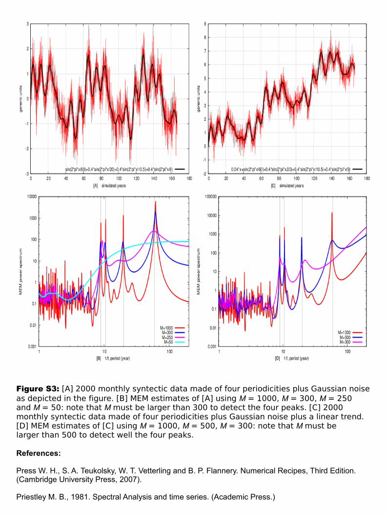
Figure S3: [A] 2000 monthly syntectic data made of four periodicities plus Gaussian noiseas depicted in the figure. [B] MEM estimates of [A] using M = 1000, M = 300, M = 250and M = 50: note that M must be larger than 300 to detect the four peaks. [C] 2000monthly syntectic data made of four periodicities plus Gaussian noise plus a linear trend.[D] MEM estimates of [C] using M = 1000, M = 500, M = 300: note that M must belarger than 500 to detect well the four peaks.

References:

Press W. H., S. A. Teukolsky, W. T. Vetterling and B. P. Flannery. Numerical Recipes, Third Edition. (Cambridge University Press, 2007).

Priestley M. B., 1981. Spectral Analysis and time series. (Academic Press.)

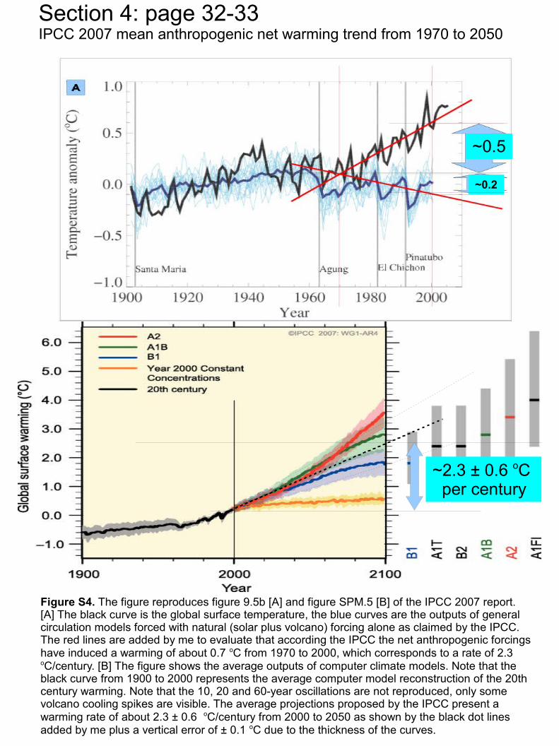
~0.5

~0.2

~2.3

Figure S4. The figure reproduces figure 9.5b [A] and figure SPM.5 [B] of the IPCC 2007 report. [A] The black curve is the global surface temperature, the blue curves are the outputs of general circulation models forced with natural (solar plus volcano) forcing alone as claimed by the IPCC. The red lines are added by me to evaluate that according the IPCC the net anthropogenic forcings have induced a warming of about 0.7 oC from 1970 to 2000, which corresponds to a rate of 2.3 oC/century. [B] The figure shows the average outputs of computer climate models. Note that the black curve from 1900 to 2000 represents the average computer model reconstruction of the 20th century warming. Note that the 10, 20 and 60-year oscillations are not reproduced, only some volcano cooling spikes are visible. The average projections proposed by the IPCC present a warming rate of about 2.3 ± 0.6 oC/century from 2000 to 2050 as shown by the black dot lines added by me plus a vertical error of ± 0.1 oC due to the thickness of the curves.

Section 4: page 32-33IPCC 2007 mean anthropogenic net warming trend from 1970 to 2050

~2.3 ± 0.6 oC per century

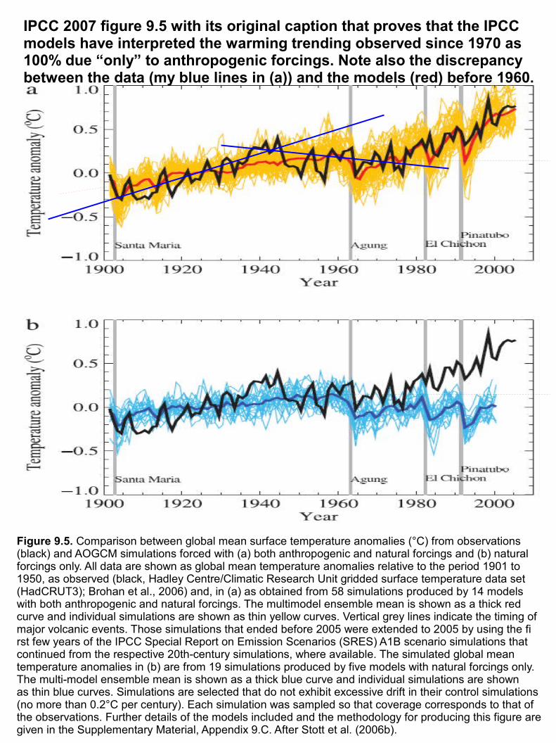
Figure 9.5. Comparison between global mean surface temperature anomalies (°C) from observations (black) and AOGCM simulations forced with (a) both anthropogenic and natural forcings and (b) natural forcings only. All data are shown as global mean temperature anomalies relative to the period 1901 to 1950, as observed (black, Hadley Centre/Climatic Research Unit gridded surface temperature data set (HadCRUT3); Brohan et al., 2006) and, in (a) as obtained from 58 simulations produced by 14 models with both anthropogenic and natural forcings. The multimodel ensemble mean is shown as a thick red curve and individual simulations are shown as thin yellow curves. Vertical grey lines indicate the timing of major volcanic events. Those simulations that ended before 2005 were extended to 2005 by using the fi rst few years of the IPCC Special Report on Emission Scenarios (SRES) A1B scenario simulations that continued from the respective 20th-century simulations, where available. The simulated global mean temperature anomalies in (b) are from 19 simulations produced by five models with natural forcings only. The multi-model ensemble mean is shown as a thick blue curve and individual simulations are shownas thin blue curves. Simulations are selected that do not exhibit excessive drift in their control simulations (no more than 0.2°C per century). Each simulation was sampled so that coverage corresponds to that of the observations. Further details of the models included and the methodology for producing this figure are given in the Supplementary Material, Appendix 9.C. After Stott et al. (2006b).

IPCC 2007 figure 9.5 with its original caption that proves that the IPCC models have interpreted the warming trending observed since 1970 as 100% due “only” to anthropogenic forcings. Note also the discrepancy between the data (my blue lines in (a)) and the models (red) before 1960.

Figure S5. The figure shows that the volcano signature reconstructed by the GCM is 2-3 times larger than what can be empirically found. In particular the log-time range effect of the volcano aerosols appears grossly overestimated. [A] Lockwood (2008) (blue) and Thompson et al. (2009) (black) empirical analyses of the volcano signature on global surface temperature against the GISS ModelE estimates (red) by (Hansen et al., 2007). [B] Filtered temperature (thin gray) vs. the three model reconstructions of the Pinatubo eruption in 1991. The figure clearly suggests that GISS ModelE overestimates the volcano signal both in amplitude and long-range duration as determined by the empirical filtering. By 2000 the volcano signature in the empirical studies vanishes.

Section 5: page 34Overestimation of the GISS ModelE reconstruction of the volcano signature

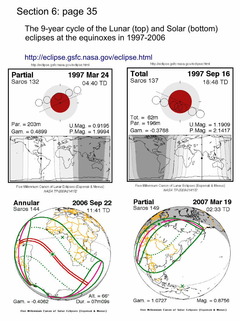
Section 6: page 35 The 9-year cycle of the Lunar (top) and Solar (bottom)

eclipses at the equinoxes in 1997-2006

http://eclipse.gsfc.nasa.gov/eclipse.html

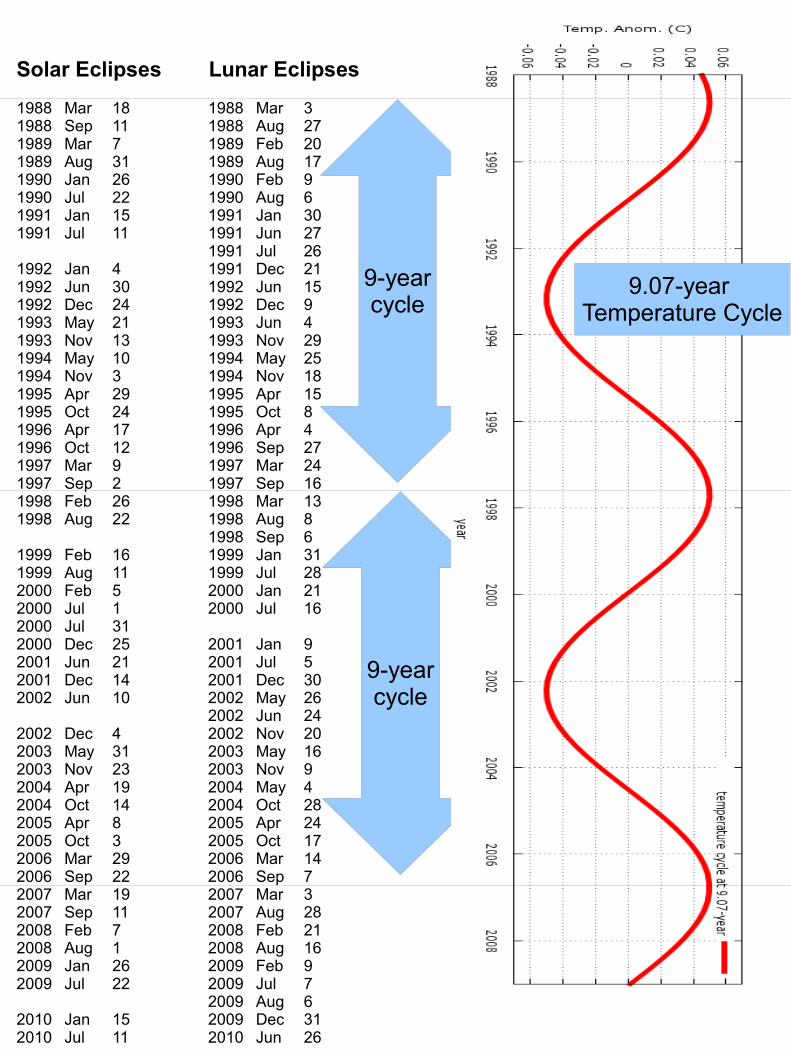
Solar Eclipses Lunar Eclipses1988 Mar 18 1988 Mar 31988 Sep 11 1988 Aug 271989 Mar 7 1989 Feb 201989 Aug 31 1989 Aug 171990 Jan 26 1990 Feb 91990 Jul 22 1990 Aug 61991 Jan 15 1991 Jan 301991 Jul 11 1991 Jun 27

1991 Jul 261992 Jan 4 1991 Dec 211992 Jun 30 1992 Jun 151992 Dec 24 1992 Dec 91993 May 21 1993 Jun 41993 Nov 13 1993 Nov 291994 May 10 1994 May 251994 Nov 3 1994 Nov 181995 Apr 29 1995 Apr 151995 Oct 24 1995 Oct 81996 Apr 17 1996 Apr 41996 Oct 12 1996 Sep 271997 Mar 9 1997 Mar 241997 Sep 2 1997 Sep 161998 Feb 26 1998 Mar 131998 Aug 22 1998 Aug 8

1998 Sep 61999 Feb 16 1999 Jan 311999 Aug 11 1999 Jul 282000 Feb 5 2000 Jan 212000 Jul 1 2000 Jul 162000 Jul 312000 Dec 25 2001 Jan 92001 Jun 21 2001 Jul 52001 Dec 14 2001 Dec 302002 Jun 10 2002 May 26

2002 Jun 242002 Dec 4 2002 Nov 202003 May 31 2003 May 162003 Nov 23 2003 Nov 92004 Apr 19 2004 May 42004 Oct 14 2004 Oct 282005 Apr 8 2005 Apr 242005 Oct 3 2005 Oct 172006 Mar 29 2006 Mar 142006 Sep 22 2006 Sep 72007 Mar 19 2007 Mar 32007 Sep 11 2007 Aug 282008 Feb 7 2008 Feb 212008 Aug 1 2008 Aug 162009 Jan 26 2009 Feb 92009 Jul 22 2009 Jul 7

2009 Aug 62010 Jan 15 2009 Dec 312010 Jul 11 2010 Jun 26

9-yearcycle

9-yearcycle

9.07-year Temperature Cycle

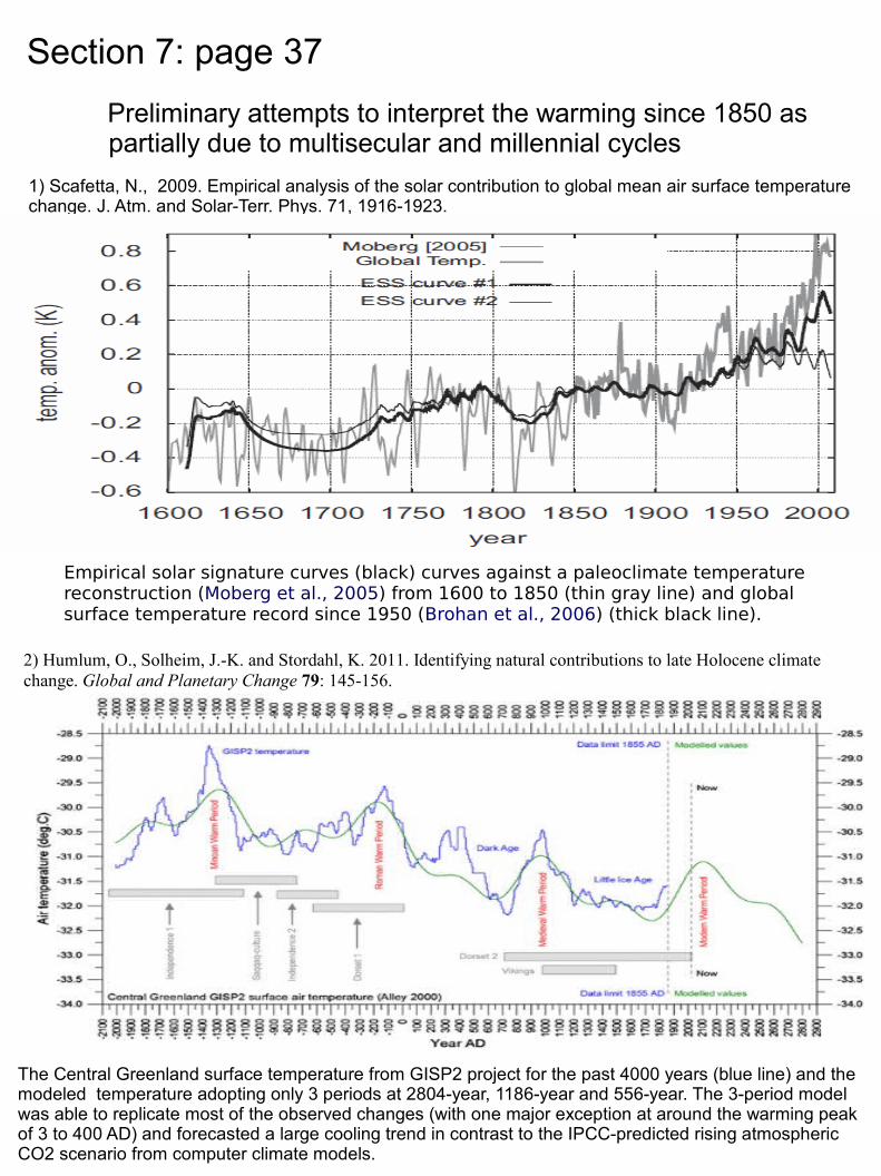
Section 7: page 37 Preliminary attempts to interpret the warming since 1850 as

partially due to multisecular and millennial cycles 1) Scafetta, N., 2009. Empirical analysis of the solar contribution to global mean air surface temperature change. J. Atm. and Solar-Terr. Phys. 71, 1916-1923.

2) Humlum, O., Solheim, J.-K. and Stordahl, K. 2011. Identifying natural contributions to late Holocene climate change. Global and Planetary Change 79: 145-156.

The Central Greenland surface temperature from GISP2 project for the past 4000 years (blue line) and the modeled temperature adopting only 3 periods at 2804-year, 1186-year and 556-year. The 3-period model was able to replicate most of the observed changes (with one major exception at around the warming peak of 3 to 400 AD) and forecasted a large cooling trend in contrast to the IPCC-predicted rising atmospheric CO2 scenario from computer climate models.

Empirical solar signature curves (black) curves against a paleoclimate temperature reconstruction (Moberg et al., 2005) from 1600 to 1850 (thin gray line) and global surface temperature record since 1950 (Brohan et al., 2006) (thick black line).

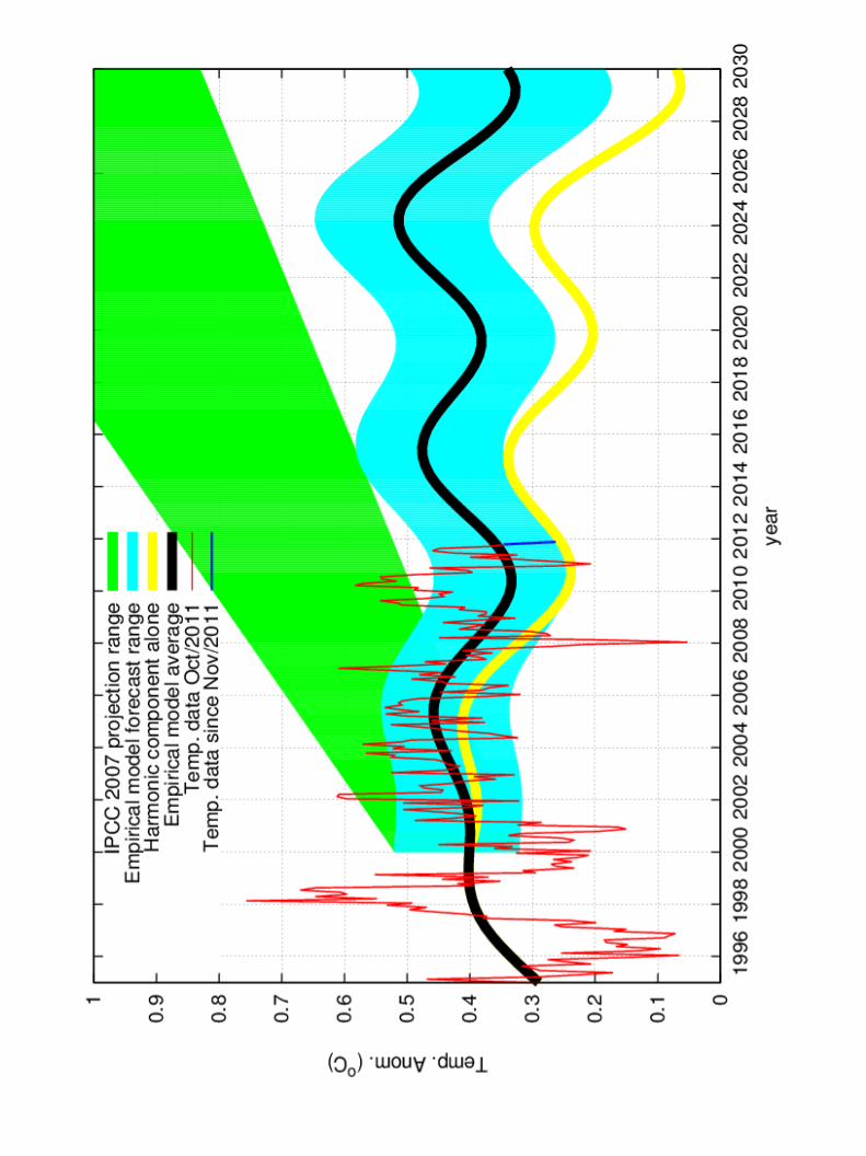
Cover photo of our solar system, as posted to inquisitor.com.