Test Collection Reliability: A Study of Bias and ...mtg.upf.edu/system/files/publications/064-test-collection-reliability-study-bias... · curacy and propose unbiased statistical

Noname manuscript No.(will be inserted by the editor)

Test Collection Reliability:A Study of Bias and Robustness to StatisticalAssumptions via Stochastic Simulation

Julian Urbano

Received: 3 May 2015 / Accepted: 14 October 2015

Abstract The number of topics that a test collection contains has a direct im-pact on how well the evaluation results reflect the true performance of systems.However, large collections can be prohibitively expensive, so researchers are boundto balance reliability and cost. This issue arises when researchers have an existingcollection and they would like to know how much they can trust their results, andalso when they are building a new collection and they would like to know howmany topics it should contain before they can trust the results. Several measureshave been proposed in the literature to quantify the accuracy of a collection toestimate the true scores, as well as different ways to estimate the expected ac-curacy of hypothetical collections with a certain number of topics. We can findad-hoc measures such as Kendall tau correlation and swap rates, and statisticalmeasures such as statistical power and indexes from generalizability theory. Eachmeasure focuses on different aspects of evaluation, has a different theoretical basis,and makes a number of assumptions that are not met in practice, such as normal-ity of distributions, homoscedasticity, uncorrelated effects and random sampling.However, how good these estimates are in practice remains a largely open question.

In this paper we first compare measures and estimators of test collection ac-curacy and propose unbiased statistical estimators of the Kendall tau and tau APcorrelation coefficients. Second, we detail a method for stochastic simulation ofevaluation results under different statistical assumptions, which can be used for avariety of evaluation research where we need to know the true scores of systems.Third, through large-scale simulation from TREC data, we analyze the bias ofa range of estimators of test collection accuracy. Fourth, we analyze the robust-ness to statistical assumptions of these estimators, in order to understand whataspects of an evaluation are affected by what assumptions and guide in the de-velopment of new collections and new measures. All the results in this paper arefully reproducible with data and code available online.

Keywords Information Retrieval · Evaluation · Test Collection · Reliability ·Simulation

J. UrbanoUniversitat Pompeu Fabra, SpainE-mail: [email protected]

2 Julian Urbano

1 Introduction

The purpose of evaluating an Information Retrieval (IR) system is to predict howwell it would satisfy real users. The main tool used in these evaluations are testcollections, comprising a corpus of documents to search, a set of topics, and aset of relevance judgments with information as to what documents are relevantto the topics (Sanderson 2010). Given the documents returned by a system fora topic, effectiveness measures like Average Precision are used to score systemsbased on the relevance judgments. After running the systems with all topics inthe collection, the average score is reported as the main indicator of system effec-tiveness, estimating the expected performance of the system for an arbitrary newtopic. When comparing two systems, the main indicator reported is the averageeffectiveness difference, based on which we conclude which system is better.

A question raises immediately: how reliable are our conclusions about systemeffectiveness? (Tague-Sutcliffe 1992). Ideally, we would evaluate systems with allpossible topics that users might conceive; this would imply that the true meanperformance of the systems corresponds to the observed mean scores computedwith the collection. But sure enough, building such a collection is either impracticalfor requiring an enormous amount of topics and relevance judgments, or just plainimpossible if the potential set of topics is infinite or not well-defined. Therefore, thetopics in a test collection must be regarded as a sample from a universe of topics,and the observed mean scores as mere estimates of the true means, erroneousto some degree. The results may change drastically with a different topic set,so much that differences between systems could even be reversed. This issue isclosely related to the statistical precision of our estimates. If D1, D2, . . . are thedifferences observed between two systems with a test collection, we know that theobserved mean D bears some random error due to the sampling of topics. In fact,its sampling distribution has variance σ2(D)/nt, where nt is the number of topics,clearly showing that our confidence in the conclusions depend not only on theobserved score, but also on the variability and the number of topics used. If theobserved difference is large, or the variability small, we can be confident that it isreal. If not, we need to increase the number of topics to gain statistical precision.

We are therefore interested in quantifying and minimizing the estimation er-ror. On the one hand, researchers want to estimate how well the results from anexisting collection reflect the true scores of systems, that is, the accuracy of thecollection. On the other hand, they want to estimate the expected accuracy of acollection with a certain number of topics, that is, the reliability of a collectiondesign. A number of papers in the last fifteen to twenty years have studied thisissue of IR evaluation. Early work suggested the use of ad hoc, easy to under-stand measures for assessing the accuracy of a test collection, such as the Kendallτ correlation (Voorhees 1998; Kekalainen 2005; Sakai and Kando 2008), swaprates (Buckley and Voorhees 2000; Sakai 2007), sensitivity (Voorhees and Buck-ley 2002; Sanderson and Zobel 2005; Sakai 2007) or the newer Average Precisioncorrelation (Yilmaz et al 2008) and drank distance (Carterette 2009). Some oth-ers suggested the use of measures based on statistical theory, such as proceduresfor significance testing (Hull 1993; Zobel 1998; Sakai 2006; Smucker et al 2009)coupled with power analysis (Webber et al 2008; Sakai 2014a,b) or classical testtheory and generalizability theory (Bodoff and Li 2007; Carterette et al 2009).Urbano et al (2013b) recently reviewed many of these measures and found that

Test Collection Reliability: Bias and Robustness 3

they can be quite unstable. They also found clear discrepancies among measures,as already observed for instance by Sakai (2007).

All measures quantify in some way how close the scores observed with a testcollection are to the true scores. The problem though, is that in practice we do notknow the true system scores, so much of the previous work was devoted to developestimators from existing data. Ad hoc measures are not founded on statisticaltheory, so they are estimated through extrapolation of the trends observed withrandomized topic set splits, as if one were the actual collection and the otherone were the true scores. Statistical measures, on the other hand, are estimatedvia inference using simple equations parameterized by the topic set size. All pastresearch is thus limited in the sense that we do not know how accurate theseestimators really are, because we just do not know the true system scores andtherefore we can not know how close our estimates are to the true accuracy of thecollections. This is a very important issue in practice, because these estimatorscould be biased and tell us that collections are more accurate than they really are,or that some fixed number of topics is more reliable than it actually is; we just donot know. For instance, it is impossible to know the true Type I and Type II errorsof significance tests (Cormack and Lynam 2006), so we resort to approximationssuch as conflict ratios similarly computed through split-half designs (Zobel 1998;Sanderson and Zobel 2005; Voorhees 2009; Urbano et al 2013a).

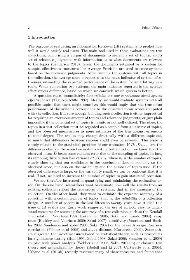
This is particularly important for statistical measures, because they make anumber of assumptions that are, by definition, not met in IR evaluation exper-iments (van Rijsbergen 1979; Hull 1993). The main reason is that effectivenessmeasures produce discrete values typically bounded by 0 and 1 (Carterette 2012).For instance, some measures of collection accuracy assume that score distribu-tions are normally distributed1; they are not because they are bounded. Othermeasures assume homoscedasticity, that is, equal variance across systems. Webberet al (2008) showed that IR evaluations violate this assumption as well, whichcan be derived again from the fact that scores are bounded. Another typical as-sumption is that effects are uncorrelated, which again does not hold because of thebounds2. Finally, all measures assume that the topics are a (uniform) random sam-ple from the universe of topics and therefore constitute a representative sample.While it is fair to assume random samples in practice, the process by which topicsare created may result in biased samples because they are created by humans whoincorporate their own biases into the collection (Voorhees 1998). In IR evaluation,we thus find non-normal distributions, heteroscedasticity, correlated effects and,usually, random sampling. Fig. 1 shows some examples.

In this paper we study all these issues of test collection reliability. Our maincontributions are:

– A discussion about the concepts of accuracy and reliability of IR test collec-tions. We review several measures to quantify the accuracy of collections, aswell as estimators of the accuracy of an existing collection, and the expectedaccuracy of a particular collection design.

– To overcome the problem of not knowing the true system scores, we propose analgorithm for stochastic simulation of evaluation results where the true system

1 Actually, they assume that the residuals are normal, not the score distributions.2 Some models assume independence, which is an even stronger assumption. The statistical

measures we review assume uncorrelated effects, but not independence.

4 Julian Urbano

Observed scores

Reciprocal Rank

Den

sity

0.0 0.2 0.4 0.6 0.8 1.0

01

23

4

Residuals

Reciprocal Rank

Den

sity

−0.6 −0.2 0.2 0.4 0.6

0.0

0.5

1.0

1.5

●

●

●

●

● ●

● ●

●●

●

●

●

●

●

●

●

●

●

●

●

●●

● ●

●

●

●

● ●

●

●

●●

●●

● ●

●

●

●

●

●

●●

●

●

●

●

−0.2 0.0 0.1 0.2 0.3

−0.

40.

00.

20.

4

Correlated effects

Topic effect

Sys

tem

res

idua

l

●●

●

●

● ●

●

●

●

●

●

●

●

●

●

●●

●●

●

●●

●

●

●●

●

●

●

●

●

●

●

●

●

●●

●

●

●

●

●●

●

●● ●

●

●

−0.4 −0.2 0.0 0.2−

0.6

−0.

20.

2

Correlated systems

Residual of first system

Res

idua

l of s

econ

d sy

stem

Fig. 1 Examples of violations of statistical assumptions in some TREC systems. Top: clearlynon-normal distribution of Reciprocal Rank scores for a system, and the corresponding residu-als that closely resemble a normal distribution; the red line is the density function of a normaldistribution with the same variance and mean zero. Bottom: correlation between topic meanscores and system residuals, and between the residuals of two systems. See Sect. 3.2 for thedefinition of these effects.

scores are fixed upfront. It simulates a collection of arbitrary size from a givencollection representing the systems and universe of topics to simulate from.The algorithm can simulate collections under all combinations of the aboveassumptions, and we show that it produces realistic results.

– Through large-scale simulation, we quantify for the first time the bias of theestimators of Kendall τ , τAP , Eρ2 and other measures of test collection accu-racy. In fact, we show that the traditional estimators are biased and tend tounderestimate the true accuracy of collections.

– We also study how robust these estimators are to the assumptions of normality,homoscedasticity, uncorrelated effects and (uniform) random sampling. Ourresults show that the first two do not seem to affect IR evaluation, and thatthe effect of non-random sampling appears to be minor.

– We propose two statistical estimators of the Kendall τ and τAP correlations,called Eτ and EτAP , and show that they are unbiased and behave much betterthan the typical split-half extrapolations.

The remainder of the paper is organized as follows. In Sect. 2 we review theconcepts of accuracy and reliability applied to IR evaluation, in Sect. 3 we re-view several ad hoc and statistical measures proposed in the literature, and inSect. 4 we discuss how they are estimated from past data. In Sect. 4.3 we pro-pose Eτ and EτAP . In Sect. 5 we propose the algorithm for stochastic simulationof evaluation results. Through large-scale simulation from past TREC data, inSect. 6 we review the bias of the estimators of the accuracy of an existing col-lection, and in Sect. 7 we review their bias to estimate the accuracy of a newcollection of arbitrary size; in both sections, we also review their robustness tostatistical assumptions. Finally, in Sect. 8 and 9 we finish with a discussion ofresults, the conclusions of the paper and proposals for further research. All the


results in this paper are fully reproducible with data and code available online athttp://github.com/julian-urbano/irj2015-reliability.

2 Evaluation Accuracy and Reliability

Let us consider a first scenario where a researcher wants to evaluate a fixed setof ns systems and there is a test collection X available with nt topics. Let µ bethe vector of ns true mean scores of the systems according to some effectivenessmeasure. Our goal when using the collection X is to estimate those true scoresaccurately, and this accuracy may be defined differently depending on the needsand goals of the researcher. For example, if we were interested in the absolute meanscores of the systems, we could define accuracy as the mean squared error oversystems: MSE(X,µ) = 1

ns

∑s (Xs − µs)2. If we were interested just in the ranking

of systems, we could use the Kendall τ correlation coefficient instead. In general,we can define accuracy as a function A that compares the results of a given testcollection with the true scores. The problem is that we can not compute the actualaccuracy A(X,µ) because the true system scores are unknown. The approach hereis to use some function fA as an estimator of the collection accuracy:

A(X,µ) = fA(X). (1)

The second scenario is that of a researcher building a new test collection X′

to evaluate a fixed set of ns systems, and who wants to figure out a suitablenumber of topics to ensure some level of accuracy. In this case, we are not in-terested in how accurate a particular collection is, but rather in how accurate ahypothetical collection with n′t topics is expected to be3: En′

tA(X′,µ). This expec-

tation naturally leads us to consider the reliability of a topic set size: an amountof topics can be considered reliable to the extent that a new collection of thatsize is expected to be accurate. Let us therefore define reliability as a functionRA(X, n′t,µ) = En′

tA(X′,µ). Unfortunately, we are in he same situation as be-

fore and the true system scores remain unknown. The approach is similarly to usesome function gA as an estimator of the expected collection accuracy:

RA(X, n′t,µ) = gA(X, n′t). (2)

An important characteristic of fA and gA is their bias. If we were measuringcollection accuracy in terms of the Kendall τ correlation and the estimator fA werepositively biased, we expect it to be overestimating the correlation. This wouldmean that our ranking of systems is not as close to the true ranking as fA tellsus. Similarly, gA would tell us that a certain number of topics, say 50, is expectedto produce a correlation of 0.9, when in reality it is lower. The bias is defined as:

bias(fA) = EX

[A(X,µ)−A(X,µ)

]= EX

[fA(X)−A(X,µ)

], (3)

bias(gA) = EX

[RA(X, n′t,µ)−RA(X, n′t,µ)

]= EX

[gA(X, n′t)−En′

tA(X′,µ)

]. (4)

3 We loosely use the notation Erf(X) to refer to the expected value of f(X) over thepopulation, restricted by r, from which X is sampled.

6 Julian Urbano

and we expect bias(fA) = bias(gA) = 0.In the following section we review different measures of accuracy and then show

how they are estimated with different fA and gA functions. We will see that inpractice fA(X) is defined4 as gA(X, |X|), so if gA is biased so will be fA.

3 Measures of Evaluation Accuracy

As mentioned earlier, we can follow different criteria to quantify how well a testcollection is estimating the true system scores. We may compute the absolute errorof the mean system scores, the ranking correlation, or even test for statistical sig-nificance. In the following subsections we review different measures of the accuracyof an IR test collection.

3.1 Ad hoc Measures

These measures are based on the concept of a swap between two systems, that is,according to the observed scores one system is better than another one when, inreality, it is the other way around. Some measures are borrowed or adapted fromother fields, such as the Kendall correlation or the Average Precision correlation,while others like sensitivity are specifically defined for IR.

3.1.1 Kendall tau correlation: τ

The Kendall τ correlation coefficient measures the correlation between the tworankings of ns systems, computed as the fraction of pairs that are in the same orderin both rankings (concordant) minus the fraction that are swapped (discordant):

τ =#concordant−#discordant

ns(ns − 1)/2. (5)

It thus ranges between -1 (reversed ranking) and +1 (same ranking). In Infor-mation Retrieval, Kendall τ is widely used to measure the similarity between therankings of systems produced by two different evaluation conditions, such as dif-ferent assessors (Voorhees 1998), effectiveness measures (Kekalainen 2005), topicsets (Carterette et al 2009) or pool depths (Sakai and Kando 2008). In our case,we are interested in the correlation between the ranking of systems according toa given collection and the true ranking of systems.

3.1.2 Average Precision correlation: τAP

In Information Retrieval we are often more interested in the top ranked items. Forinstance, effectiveness measures usually pay more attention to the relevance of thetop ranked documents. Similarly, we may tolerate a swap between systems at thebottom of the ranking, but not between the two best systems. Yilmaz et al (2008)proposed an extension of Kendall τ to add this top-heaviness component following

4 We use |X| to denote the number of topics in X.


the rationale behind Average Precision. Instead of comparing every system withall others, it only compares it with those ranked above it:

τAP =2

ns − 1

ns∑s=2

(C(s)

s− 1

)− 1, (6)

where C(s) is the number of systems above rank s correctly ranked with respectto the system at that rank. Note that τAP similarly ranges between -1 and +1, butit penalizes swaps towards the top of the ranking more than towards the bottom,making it a more appealing alternative for IR evaluation.

3.1.3 Absolute and Relative Sensitivity: sensabs and sensrel

If the observed difference between two systems is large, it is unlikely that their truedifference has a different sign, because the likelihood of a swap is inversely propor-tional to the magnitude of the difference. Therefore, another view of accuracy isestablishing a threshold such that if the observed difference between two systemsis larger, the probability of actually having a swap is kept below some level like5% (Voorhees and Buckley 2002; Buckley and Voorhees 2000). Of course, we wantthat threshold to be as small as possible, meaning that we can trust the sign ofmost of the observed differences. The smallest threshold that ensures a maximumswap rate is called the sensitivity of the collection.

Sanderson and Zobel (2005) pointed out that differences between systems areoften reported in relative terms rather than absolute (eg. +12% instead of +0.032),so we may also be interested in the relative sensitivity of a test collection. In thispaper, we set the maximum swap rate to 5%, and refer to absolute and relativesensitivity as sensabs and sensrel.

3.2 Statistical Measures

The ad hoc measures of collection accuracy are concerned with possible swapsbetween systems, but they neglect the magnitude of their differences as well astheir variability. However, the probability of a swap is inversely proportional tothe true difference between systems and proportional to their variability: if theobserved difference is too small or too variable, they are likely to be swapped. Thestatistical measures described in the following are all based on the decomposition ofthe variance of the observed scores. Throughout this section we follow the notationtraditionally used in generalizability theory (Brennan 2001; Bodoff and Li 2007).

Because we have a fully crossed experimental design (i.e., all systems evaluatedwith the same topics), we can consider the following random effects model for theeffectiveness of system s on topic t:

Xst = µ+ νs + νt + νst, (7)

where µ is the grand mean score of all systems in the universe of topics, νs = µs−µand νt = µt − µ are the system and topic effects, and νst is the interaction effectthat would correspond to the residual effect. Note that a system effect is defined asthe deviation of its true mean score µs from the grand average µ, so a system withbetter (worse) performance than average has a positive (negative) system effect.

8 Julian Urbano

Topics are defined similarly, that is, a hard (easy) topic has a negative (positive)topic effect. The residual effects just model the system-topic interactions, wheresome systems are particularly good or bad for certain topics. For each effect inEq. (7) there is an associated variance of that effect, called the variance component:

σ2(s) = Esν2s , σ2(t) = Etν

2t , σ2(st) = EsEtν

2st. (8)

Because the effects are defined by subtracting the grand mean µ, they are alluncorrelated and centered at zero. Therefore, the total variance of the observedscores can be decomposed into the following components:

σ2(Xst) = EsEt(Xst − µ)2 = σ2(s) + σ2(t) + σ2(st). (9)

Note that this total variance is the variance for single systems on single topics.However, researchers compare systems based on their mean performance over thesample of topics in a test collection. The linear model for the decomposition of asystem’s average score over a sample of topics is

XsT = Xs = µ+ νs + νT + νsT , (10)

which is analogous to Eq. (7) except that the index of a topic t is replaced by Tto indicate the mean over a set of topics. From the above model, we can see thatthe true mean score of a system s is the expected value, over randomly parallelsets of topics, of the observed mean scores:

µs = ETXsT . (11)

Because the νT and νsT effects involve the mean over a set of nt independenttopics from the same universe, their corresponding variance components are

σ2(T ) = ET ν2T =

σ2(t)

nt, σ2(sT ) = EsET ν

2sT =

σ2(st)

nt, (12)

and as in Eq. (9), the variance of the observed mean scores is decomposed into

σ2(XsT ) = EsET (XsT − µ)2 = σ2(s) + σ2(T ) + σ2(sT ). (13)

From Eq. (13) we can see that the variability of the observed mean scores is de-composed into the inherent variability among systems, the variability of the meantopic difficulties, and the variability of the mean system interaction with topics.The following measures of collection accuracy are defined from these components.

3.2.1 Generalizability Coefficient: Eρ2

Using the above decompositions in variance components, one can define differentmeasures of accuracy based on the concept of correlation. Let Q be true scores ofsome quantity of interest, such as the true mean effectiveness of systems. A testcollection provides us with estimates Q = Q + e, bearing a certain random anduncorrelated error e. Their correlation is

ρ(Q,Q) =cov(Q,Q)

σ(Q)σ(Q)=

cov(Q+ e,Q)

σ(Q)σ(Q)=

σ2(Q)

σ(Q)σ(Q)=σ(Q)

σ(Q). (14)


If we take the square of the correlation, this conveniently simplifies to a ratio ofvariance components:

ρ2(Q,Q) =σ2(Q)

σ2(Q)=

σ2(Q)

σ2(Q+ e)=

σ2(Q)

σ2(Q) + σ2(e). (15)

Therefore, one can define a measure of accuracy for some arbitrary quantity ofinterest as the squared correlation between the true scores and the estimatedscores which, in turn, can be easily defined as the variance of the true scores toitself plus error variance (Allen and Yen 1979).

In IR evaluation experiments, we are often interested in the relative differencesamong systems, that is, in the system deviation scores µs − µ. When using a testcollection, we estimate this quantity with XsT − µT , so the error of our estimatesand its variance are

δs = (XsT − µT )− (µs − µ) = νsT , (16)

σ2(δ) = σ2(sT ). (17)

Plugging into Eq. (15), we get the following accuracy measure for our estimatesof relative system scores (Brennan 2001):

Eρ2 = ρ2(XsT − µT , µs − µ) =σ2(s)

σ2(s) + σ2(sT ). (18)

In generalizability theory literature, this measure is called generalizability co-efficient. Cronbach et al (1972) introduced the notation Eρ2 to indicate that thiscoefficient is approximately equal to the expected value, over randomly parallelcollections of nt topics, of the squared correlation between observed and true scores(note that this definition is already concordant with our definition of reliability).

3.2.2 Dependability Index: Φ

Sometimes, a researcher is not interest in the system deviation score µs − µ, butrather in its deviation from a domain-dependent criterion λ, such as the meaneffectiveness of a baseline. In this case, our estimate is XsT − λ, so the error andits variance are

∆s = (XsT − λ)− (µs − λ) = XsT − µs = νT + νsT , (19)

σ2(∆) = σ2(T ) + σ2(sT ). (20)

Plugging into Eq. (15), we get the following accuracy measure for our criterion-referenced estimates of system performance (Brennan 2001):

ρ2(XsT − λ, µs − λ) =σ2(µs − λ)

σ2(µs − λ) + σ2(T ) + σ2(sT ).

Because the quantity of interest here is the deviation from a fixed criterion λ,this measure does include the topic effect, which enters the absolute error variance.In the above case of deviation from the observed mean score µT , the topic effectdid not enter the error variance in Eq. (18) because it is the same for all systems.

10 Julian Urbano

In the special case when λ = µ, this measure is called the dependability index Φ(Brennan and Kane 1977):

Φ = ρ2(XsT − µ, µs − µ) =σ2(s)

σ2(s) + σ2(T ) + σ2(sT ). (21)

Intuitively, Φ is lower than Eρ2 because it involves not only system differences,but also topic difficulties. That is, it involves the estimation of absolute systemscores rather than just relative differences among them.

3.2.3 F -Test

Another view of reliability is given by null hypothesis testing (Hull 1993). In thegeneral case where we compare ns systems, we may state the null hypothesiswhereby all systems have the same true mean scores:

H0 : µ1 = µ2 = · · · = µns .

After evaluating all systems with a test collection, we may test this hypothesis insearch for evidence that at least one of the systems has a different mean from theothers. A common test to use here is the F -test, which involves a decompositionin variance components as well. In its general form, the F statistic is defined asthe ratio of explained variance to residual variance, which in our case is

F =explained variance

residual variance=

between-system variance

within-system variance. (22)

The numerator is defined as the between systems mean squares, while the denom-inator is the within systems or error mean squares. Their definition depends onthe variance decomposition. With one-way ANOVA, the experimental design onlyconsiders the system effect, so the topic effect is confounded with the error. In two-way ANOVA (equivalent to the above variance decomposition), the experimentaldesign considers both the system and topic effects, so the error mean square isconsiderably lower (see Sect. 4.2 for details).

Under the null hypothesis, the F statistic in Eq. (22) follows an F distributionparameterized by the degrees of freedom in the numerator and in the denominator.If the observed statistic is larger than the critical value corresponding to thosedegrees of freedom and a pre-fixed significance level like α = 0.05, we reject the nullhypothesis that all system means are equal, evidencing that at least one of them isdifferent from the others. Under this framework, the accuracy of a collection canbe viewed dichotomously: does the F -test come up significant or not?

4 Estimation of Evaluation Accuracy

We could use generic f and g functions to estimate arbitrary measures of accuracyby using a split-half method that extrapolates observations made from previousdata. The problem is that the model used to extrapolate, as well as how we makeobservations from previous data, do not necessarily have a theoretical basis and itmight actually end up producing biased estimates. On the other hand, we couldderive estimators from statistical theory in search for desirable properties like


unbiasedness or low variance. These estimators are easily defined for statisticalmeasures of accuracy because they already incorporate the topic set size in theirformulation, but not for ad hoc measures. In the next two sections we reviewgeneric split-half estimators for arbitrary measures, and statistical estimators ofthe statistical measures. In Sect. 4.3 we then propose statistical estimators of theKendall τ and τAP correlations that, as we will see, behave better than the genericsplit-half estimators.

4.1 Extrapolation from Split-Half

A generic estimator found in the literature is based on the extrapolation of theobserved accuracy scores over random splits of the available topic set, such asin (Zobel 1998; Voorhees 1998; Voorhees and Buckley 2002; Lin and Hauptmann2005; Sanderson and Zobel 2005; Voorhees 2009; Urbano et al 2013a). Let X be thematrix of effectiveness scores already available to us from an existing collectionwith nt topics. The estimator randomly selects two disjoint subsets of n topicseach, leading to X′ and X′′, and then computes the accuracy A(X′,X′′T ) assumingthat the mean scores observed with X′′ correspond to the true scores. Running thisexperiment several times, the mean observed score A is taken as an estimate of theexpected accuracy of a random set of n topics from the same universe. If we repeatthis experiment for subsets of n = 1, 2, . . . , nt/2 topics, we can estimate the relationbetween accuracy and topic set size. Fitting a model to these observed scores, wecan extrapolate to the expected accuracy of a collection with an arbitrary numberof topics. In particular, we can estimate the expected accuracy of a collection of thesame size as our initial collection X. This means that we are actually estimatingA(X,µ) as RA(X, |X|,µ), that is, we are implicitly setting fA(X) = gA(X, |X|).

The extrapolation error depends on the number of topics we initially havefor the splits, the number of trials we run, and the model to interpolate. In thispaper, we run a maximum total of 1,000 trials for a given initial collection, fortopic subsets of at most 20 different and equidistant sizes, and 100 random trialsat most for each size. For instance, if we had nt=10 previous topics, we would run100 random trials at sizes n= 2, 3, 4, 5, for a total of 400 observations. If we hadnt=100 previous topics, we would run 50 random trials of sizes n=3, 6, . . . , 48, 50,for a total of 1,000 observations. Regarding the interpolation model, we test threealternatives:

exp1: gA(X, nt) = a · nbt , (23)

exp2: gA(X, nt) = a · exp(b · nt), (24)

logit: logit(gA(X, nt)) = a · log(nt) + b, (25)

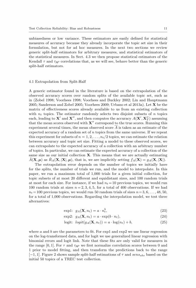
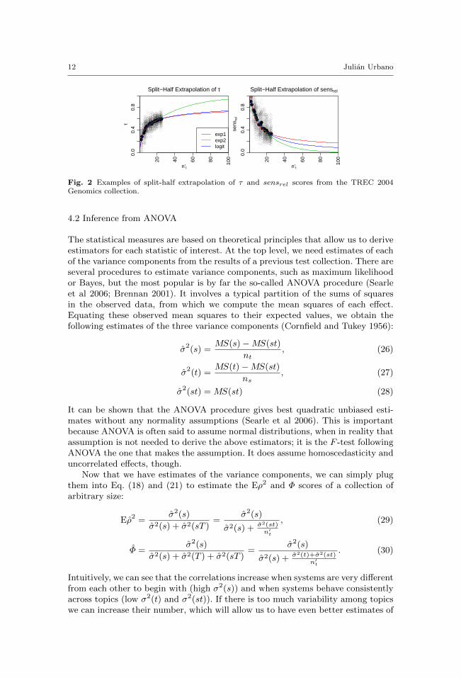
where a and b are the parameters to fit. For exp1 and exp2 we use linear regressionon the log-transformed data, and for logit we use generalized linear regression withbinomial errors and logit link. Note that these fits are only valid for measures inthe range [0, 1]. For τ and τAP we first normalize correlation scores between 0 and1 prior to model fitting, and then transform the predictions back to the range[−1, 1]. Figure 2 shows sample split-half estimations of τ and sensabs based on theinitial 50 topics of a TREC test collection.

12 Julian Urbano

20 40 60 80 100

0.0

0.4

0.8

Split−Half Extrapolation of τ

n't

τ

●●

●●●●●

●●●●●●●●●

●●●●

exp1exp2logit

20 40 60 80 100

0.0

0.4

0.8

Split−Half Extrapolation of sensrel

n't

sens

rel

●●

●●●●●

●●●●

●●●●●

●●●●

Fig. 2 Examples of split-half extrapolation of τ and sensrel scores from the TREC 2004Genomics collection.

4.2 Inference from ANOVA

The statistical measures are based on theoretical principles that allow us to deriveestimators for each statistic of interest. At the top level, we need estimates of eachof the variance components from the results of a previous test collection. There areseveral procedures to estimate variance components, such as maximum likelihoodor Bayes, but the most popular is by far the so-called ANOVA procedure (Searleet al 2006; Brennan 2001). It involves a typical partition of the sums of squaresin the observed data, from which we compute the mean squares of each effect.Equating these observed mean squares to their expected values, we obtain thefollowing estimates of the three variance components (Cornfield and Tukey 1956):

σ2(s) =MS(s)−MS(st)

nt, (26)

σ2(t) =MS(t)−MS(st)

ns, (27)

σ2(st) = MS(st) (28)

It can be shown that the ANOVA procedure gives best quadratic unbiased esti-mates without any normality assumptions (Searle et al 2006). This is importantbecause ANOVA is often said to assume normal distributions, when in reality thatassumption is not needed to derive the above estimators; it is the F -test followingANOVA the one that makes the assumption. It does assume homoscedasticity anduncorrelated effects, though.

Now that we have estimates of the variance components, we can simply plugthem into Eq. (18) and (21) to estimate the Eρ2 and Φ scores of a collection ofarbitrary size:

Eρ2 =σ2(s)

σ2(s) + σ2(sT )=

σ2(s)

σ2(s) + σ2(st)n′

t

, (29)

Φ =σ2(s)

σ2(s) + σ2(T ) + σ2(sT )=

σ2(s)

σ2(s) + σ2(t)+σ2(st)n′

t

. (30)

Intuitively, we can see that the correlations increase when systems are very differentfrom each other to begin with (high σ2(s)) and when systems behave consistentlyacross topics (low σ2(t) and σ2(st)). If there is too much variability among topicswe can increase their number, which will allow us to have even better estimates of


system effectiveness. As with the split-half estimators, the above equations are alsoused to estimate the accuracy of an existing collection as the expected accuracy ofa hypothetical collection of the same size. This means that we are again estimatingA(X,µ) as RA(X, |X|,µ), that is, we are implicitly setting fA(X) = gA(X, |X|).

For the accuracy of a collection in terms of the F -test, we can use the abovemean squares to compute the F statistic

F =MS(s)

MS(st), (31)

which, under the null hypothesis, follows and F distribution with ns − 1 andns(nt − 1) degrees of freedom. Intuitively, if the systems are very different fromeach other (high numerator), or if there is low error variance because systems donot vary too much across topics (low denominator), the F -test is more likely tocome up statistically significant.

Under the framework of significance testing, the expected accuracy of a testcollection corresponds to the statistical power of the test (Webber et al 2008).In order to estimate the power of a new collection with n′t topics, we need tospecify a target effect size. Sakai (2014a) proposed the use of a minimum detectabledifference δmin between the best and the worst systems, assuming that all othersystems are centered in the middle. That is, the best system has an effect δmin/2,the worst system has an effect−δmin/2, and all others have effect 0. This dispersionof the system mean scores results in a between-system variance

σ2(s) =

∑s ν

2s

ns=

(δmin/2)2 + (−δmin/2)2

ns=δ2min2ns

(32)

which, standardized with the within-system variance, results in the following targeteffect size for power analysis:

F1 =δ2min

2nsσ2(st). (33)

The square root of this effect size is coined f1 by Cohen (1988). We must notethat the dispersion of mean system scores assumed above is the one that yields thesmallest between-system variance, and hence the one that yields the least statis-tical power. That is, it assumes the worst case scenario where all but two systemshave the same mean, but in practice they spread near uniformly throughout therange. Cohen (1988) defines another two effect sizes assuming intermediate andmaximum between-system variance for a given δmin.

For simplicity, we use this effect size in our experiments, but stress again thatit contemplates a worst-case scenario that will inevitably underestimate reliability;we leave the topic of appropriate effect size selection for further study. We finallynote that the variance decomposition we employ is based on two-way ANOVAbecause we account for the topic effect as well. This results in a smaller error vari-ance and therefore in higher statistical power than with one-way ANOVA, whichconfounds the topic and residual effects. In this sense, our estimates are more inline with (Sakai 2014b) than with (Sakai 2014a)5. Following the traditional sugges-tion by Sparck Jones (1974), we set δmin = 0.05 to detect noticeable differences.

5 In both papers, Sakai uses total variance rather than error variance in the denominatorof F1, so statistical power is even more underestimated and there is virtually no differencebetween one- and two-way ANOVA. Sakai (2015) reports the results with error variance.

14 Julian Urbano

Note though that this threshold is arbitrary. Urbano and Marrero (2015) recentlysuggested an approach to define meaningful thresholds based on expectations ofuser satisfaction, but we leave the choice of thresholds to future research.

4.3 Statistical Estimation of Kendall τ and τAP

Even though Kendall τ and τAP are two very popular measures in IR evaluation,their split-half estimation for arbitrary topic sets can become computationallyexpensive for large-scale studies. In addition, as we will see in Sect. 6 and 7, theyproduce biased estimates. To partially overcome these problems, we propose heretwo statistical estimators of τ and τAP .

For simplicity, let us assume that systems are already sorted by their meanobserved score, so that for any two systems i and j, i < j implies Xi > Xj . LetWij be a random variable that equals 1 if systems i and j are swapped (i.e. µi < µj)and 0 if they are not (i.e. µi > µj). These variables follow a Bernoulli distributionwith parameter wij equal to the probability of swap, so their expectation andvariance are simply

E[Wij ] = wij , Var[Wij ] = wij(1− wij). (34)

These probabilities can be estimated with the scores observed in an existing col-lection. Let Dt = Xit − Xjt be the difference between both systems for topic t.By the Central Limit Theorem, the sampling distribution of D is approximatelynormal when nt is large. Therefore, we can estimate wij as

wij = P (µi − µj ≤ 0) ≈ Φ(−√n′t

D

sd(D)

), (35)

where Φ is the cumulative distribution function of the standard normal distri-bution. Therefore, an existing collection allows us to estimate the variability ofthe differences between systems (i.e. sd(D)), which we can use to estimate theprobability that systems will be swapped with an arbitrary number of topics n′t.

4.3.1 Expected Kendall τ correlation: Eτ

The Kendall τ correlation can be formulated in terms of concordant pairs alone:

τ =#concordant−#discordant

n(n− 1)/2=

2 ·#concordant

n(n− 1)/2− 1, (36)

which for our purposes would be defined as:

τ =4∑i=1

∑j=i+1 1−Wij

ns(ns − 1)− 1. (37)

Given a test collection, we can estimate the probability of swap between everypair of systems, so we can estimate the τ correlation as well. The expectation andvariance are

Eτ ≡ E[τ ] =4∑i=1

∑j=i+1 1− wij

ns(ns − 1)− 1, (38)

Var[Eτ ] ≈16∑i=1

∑j=i+1 wij(1− wij)

n2s(ns − 1)2

. (39)


As mentioned above, using Eq. (35) we can easily estimate the probability ofswap with an arbitrary number of topics. Thus, Eq. (38) becomes an estimatorof the expected τ correlation when using an arbitrary number of topics, that is,En′

tτ(X′,µ). Additionally, Eq. (39) allows us to compute a confidence interval as

well, but this is a line we do not explore in this paper.

4.3.2 Expected AP correlation: EτAP

The τAP correlation can also be defined in terms of concordant pairs:

τAP =2

ns − 1

∑i=2

(∑i−1j=1 1−Wij

i− 1

)− 1. (40)

Having a test collection, we can again estimate the probabilities of swap, so wecan estimate the τAP correlation as well. Expectation and variance are

EτAP ≡ E[τAP ] =2

ns − 1

∑i=2

(∑i−1j=1 1− wiji− 1

)− 1, (41)

Var[EτAP ] ≈ 4

(ns − 1)2

∑i=2

(∑i−1j=1 wij(1− wij)

(i− 1)2

). (42)

Similarly, Eq. (41) is an estimator of the expected τAP correlation when usingan arbitrary number of topics, that is, En′

tτAP (X′,µ).

5 Stochastic Simulation of Evaluation Results

In order to evaluate the possible bias of each A and R, we need to be able tocompute the true A(X,µ) scores, which means that we need to know the trueeffectiveness of systems. For instance, to assess the possible bias of the exp1 split-half estimator of the τ correlation coefficient, we actually need to compute thecorrelation between the true ranking of systems and the ranking produced by atest collection. In principle, we thus need to know the true effectiveness of systemsand a way to obtain randomly parallel test collections of varying sizes where topicsare sampled from the same universe of topics. Finally, we also want to be able tocontrol which statistical assumptions are violated in the creation of these testcollections, so we can assess the robustness of the estimators to each of theseviolations. Unfortunately, there is no way of knowing the true effectiveness ofsystems, certain assumptions are not met by definition, and there is no archiveof past evaluation data large enough to serve our needs. Instead, we resort tostochastic simulation.

Let X be the nt×ns matrix of effectiveness scores obtained by a set of systemswith an existing set of topics. Our goal is to simulate a new matrix Y with scores bythe same set of systems with a randomly parallel set of n′t topics. The complexityof course resides in making this simulation realistic. There are four main pointswe must consider:

– We need to know the exact true mean scores of systems µ, each of which mustequal XsT in expectation: µs = ETXsT , which implies µ = ETEsXsT . Thiswill allow us to compute the actual accuracy of the simulated collections.

16 Julian Urbano

– Regardless of the assumptions, topic effects must be sampled from a fixed truedistribution of the universe of topics.

– The dependence structure underlying topic and residual effects must be pre-served to maintain the possible correlations between systems and topics (seethe bottom plots in Figure 1). This will allow us to preserve the inherent simi-larity between systems by the same group, or the interaction between systemsand topic difficulty, for example.

– Even though the residual distributions can sometimes be approximated bycertain families of well-known distributions, we need to adhere to their truedistributions, especially when we do not want the homoscedasticity or normal-ity assumptions to hold.

One could just set one Beta distribution for each system and draw randomvariables, but the resulting residuals would not necessarily follow the realisticdistributions. Even if one estimates each residual distribution and draws samplesfrom those estimates, the expected topic effects would all be zero. If one alsoestimates the topic effect distribution and draws from it as well, the dependencestructure would still be ignored. In the next section we outline the method wefollow to simulate realistic evaluation results.

5.1 Outline of the Simulation Method

Algorithm 1 details the full simulation method. For the time being, let us describeit without paying attention to how statistical assumptions are dealt with; theywill be covered in Sect. 5.2. We begin by considering again the model in Eq. (7)to decompose effects in the existing collection. For our purposes, we will fix thetrue grand average and the true system effects as the observed mean scores in X(lines 5–6):

µ ≡ Xst =1

nsnt

∑s

∑t

Xst, (43)

νs = µs − µ ≡ Xs − µ =1

nt

∑t

Xst − µ (44)

Fixing µ and νs allows us to compute the actual accuracy of a simulated randomlyparallel collection Y. The following mixed effects model will serve as the basis tosimulate such collection

Yst = µ+ νs + Tt + Est, (45)

where Tt and Est are random variables corresponding to the topic and residualeffects. Let FT be the true cumulative distribution function of topic effects, letFEs

be the true cumulative distribution function of residual effects for system s,and let F−1

T and F−1Es

be their inverses (i.e., the quantile functions). Under thismodel, each topic t corresponds to a random vector (E1t, . . . , Enst, Tt) from a jointmultivariate distribution F whose marginal distributions are (FE1

, . . . , FEns, FT ).

The simulation mainly consists in generating such random vectors and pluggingthem in Eq. (45).

If we just drew independent random variables from the distributions of top-ics and residuals, we would lose their inherent correlations. To avoid this, we use


copulas. A copula is a multivariate distribution that describes the dependence be-tween random variables whose marginals are all uniform. By Sklar’s theorem, anyjoint multivariate distribution, like our F distribution, can be defined in terms ofits marginal distributions and a copula describing their dependence structure (Joe2014). Copulas are used as follows. Let (A1, A2, . . . ) be a random vector whereeach variable follows some distribution FAi

. By the probability integral transform,if we pass each of them through their distribution function, we get a random vec-tor where the marginals are uniform: Ui = FAi

(Ai) ∼ Uniform(0, 1). Now, let Cbe the copula of the multivariate distribution of (U1, U2, . . . ); it contains the de-pendence structure between all Ui and its marginals are all uniform. We can nowuse the copula to generate a random vector (R1, R2, . . . ), which maintains thedependence structure and can be transformed back to our original distribution. Inparticular, we now compute A′i = F−1

Ai(Ri) to obtain a random vector with the

same marginals: A′i ∼ FAi.

There are many families of copulas to model different types of dependencestructure. Here we will use Gaussian copulas because they are easy to work withand they maintain the correlation between variables. First, we use kernel densityestimation to estimate and fix the true marginals of the topic and residual effects;let FT and FEs

be our estimates (lines 11–12). Now, we need to generate n′t ran-dom vectors from a Gaussian copula with the same variance-covariance matrix asour topic and residual effects (note from line 13 that topic effects are appended toresidual effects). We achieve this by generating independent standard normal vec-tors and multiplying them by the Cholesky factorization of the variance-covariancematrix Σ (lines 13, 22–24). Next, we pass each of the resulting Rs vectors throughthe normal cumulative distribution function Φ with mean 0 and variance Σs,s,which results in the uniform random vectors generated from the copula (line 25).

These random vectors have the desired correlations, but not the marginalsyet, so we pass each of them through the inverse distribution function of thecorresponding residual or topic effect (line 29). Each of the resulting variablesZst (s ≤ ns) corresponds to the residual effect of system s for the new topic t,and the Zns+1,t are the new topic effects. The simulated score Yst of system s fortopic t is computed by adding these two random effects to the fixed grand meanµ and the fixed true system effect νs (line 33).

5.2 Dealing with Statistical Assumptions

The basic algorithm presented so far allows us to simulate the effectiveness scoresobtained by a certain set of systems on an arbitrarily large set of topics from thesame universe. In this section we describe how this basic algorithm is expanded tosimulate data following various combinations of statistical assumptions.

Normality. In line 29 of the algorithm, we pass each of the random vectorsgenerated with the copula through the inverse distribution functions of the residualand topic effects, so the marginals are the same as in our original data. If we wantto force the normality assumption, all we have to do is substitute all FEs

(and theirinverses) with the normal distribution function with mean 0 and variance Σs,s, sothe resulting residuals are all normal and with the original variance (lines 26–28).Note that the transformation of the topic effects is still done with F−1

T , because thenormality assumption applies only to the residuals. If, on the other hand, we do

18 Julian Urbano

Algorithm 1 Stochastic simulation of evaluation results with n′t new topics, giventhe results with a previous test collection X.

1: function Simulate(X,n′t)2: if not normality then3: X← logit(X)4: end if5: µ← Xst

6: νs ← Xs

7: if homoscedasticity then8: σ2

p ← 1ns

∑s σ

2(Es)

9: Es ← Es/√σ2(Es) ·

√σ2p . σ2(Es) = σ2

p

10: end if

11: FT ← KernelEstimation(νt) . FT ≈ FT12: FEs ← KernelEstimation(Es) . FEs ≈ FEs

13: Σ← Cov[(E1, . . . ,Ens ,T)] . Σ ≈ Σ14: if uncorrelated effects then15: ∀i 6= j : Σij ← 016: end if

17: if random sampling then18: n′′t ← n′t19: else20: n′′t ← max(400, 4n′t)21: end if22: C← Cholesky(Σ) . Σ = CTC23: R← (R1, . . . ,Rns ,Rns+1) . |Ri| = n′′t , R ∼ Normal(0, I)

24: R← R×C . Cov[R] ≈ Σ , R ∼ Normal(0, Σ)

25: U← (Φ(R1; 0, Σ1,1), . . . , Φ(Rns+1; 0, Σns+1,ns+1)) . Ui ∼ Uniform(0, 1)

26: if normality then27: FEs ← Φ0,Σs,s

28: end if29: Z←

(F−1E1

(U1), . . . , F−1Ens

(Uns ), F−1T (Uns+1)

). Cov[Z] ≈ Σ

∀i ≤ ns : Zi ∼ FEi, Zns+1 ∼ FT

30: if not random sampling then31: Z← BetaSampling(Z, n′t)32: end if

33: Yst ← µ+ νs + Zns+1,t + Zst34: if not normality then35: Y ← logit−1(Y)36: end if37: return Y38: end function

not force the normality assumption, the residuals will have the correct marginals,but the actual scores may fall outside the [0, 1] range when adding all effects,resulting in unrealistic data. To avoid this, we first transform the original scoresX with the logit function, so the range becomes (−∞,+∞) instead of [0, 1] (lines2–4). The algorithm proceeds the same way to generate the new data Y in logitunits, and the inverse logit function is used at the end to transform the simulatedscores back to the [0, 1] range (lines 34-36). Through appropriate transformation,


0.0

0.2

0.4

0.6

0.8

1.00.

000.

040.

08

Non−random sampling of topic effects

νt quantile

Pro

babi

lity

of b

eing

sam

pled alpha = 0.01 , beta = 2

alpha = 2 , beta = 2alpha = 0.01 , beta = 8alpha = 2 , beta = 8Uniform sampling

Fig. 3 Sample Beta distributions used for non-random sampling of topic effects; they definethe probability that certain quantiles of the topic effects distribution will be sampled. Forinstance, with α = 0.01 and β = 8 (solid green line) we are most likely to select topics fromthe lower quantiles, that is, harder topics. A uniform distribution (dashed gray line) wouldachieve random sampling.

we can thus simulate data with residuals following normal distributions or realisticdistributions as in the original data.

Homoscedasticity. Because we use the variance-covariance matrix of the orig-inal data throughout the algorithm, the simulated scores have the same within-system variance as in the original data. This implies that if the original data isheteroscedastic, the simulated data will be heteroscedastic too. If we want to forcehomoscedasticity, we can re-scale all the residuals to have a common (pooled)variance σ2

p (lines 7–10). Note that the transformed residuals are still centered atzero, and the correlations among residual and topic effects do not change becausethis transformation is linear.

Uncorrelated effects. The use of copulas in the algorithm is motivated bythe observation that IR evaluation scores do present a certain level of correlationthat we want to preserve. If we still want to force uncorrelated effects we can simplyset all the off-diagonal components of the variance-covariance matrix to zero, sothat we maintain the residual variances but not their correlations (lines 14–16). Analternative is to just generate and transform independent normal random variableswith the appropriate variances instead of using the copula, but we prefer to modifythe variance-covariance matrix for simplicity.

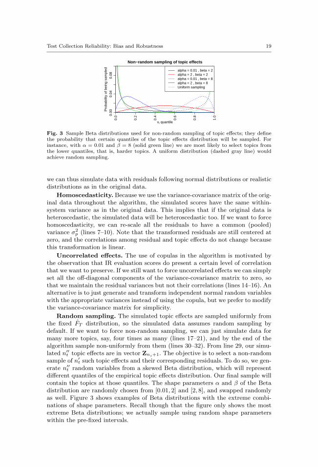
Random sampling. The simulated topic effects are sampled uniformly fromthe fixed FT distribution, so the simulated data assumes random sampling bydefault. If we want to force non-random sampling, we can just simulate data formany more topics, say, four times as many (lines 17–21), and by the end of thealgorithm sample non-uniformly from them (lines 30–32). From line 29, our simu-lated n′′t topic effects are in vector Zns+1. The objective is to select a non-randomsample of n′t such topic effects and their corresponding residuals. To do so, we gen-erate n′′t random variables from a skewed Beta distribution, which will representdifferent quantiles of the empirical topic effects distribution. Our final sample willcontain the topics at those quantiles. The shape parameters α and β of the Betadistribution are randomly chosen from [0.01, 2] and [2, 8], and swapped randomlyas well. Figure 3 shows examples of Beta distributions with the extreme combi-nations of shape parameters. Recall though that the figure only shows the mostextreme Beta distributions; we actually sample using random shape parameterswithin the pre-fixed intervals.

20 Julian Urbano

Track Measure ns nt σ2(s) σ2(t) σ2(st)Enterprise 2006 (expert) Average Precision 68 (91) 49 24% 33% 43%Genomics 2004 (ad hoc) Average Precision 35 (47) 50 6% 58% 35%Robust 2003 Average Precision 58 (78) 100 1% 80% 19%Web 2004 (home + named) Reciprocal Rank 55 (73) 150 6% 41% 53%

Table 1 Summary of the four TREC test collections used in the paper. The Enterprise,Genomics and Robust collections represent low, intermediate and high difficulty for evaluation,respectively. The Web collection merges the 75 topics for homepage finding and the 75 topicsfor named page finding. Numbers in parentheses indicate the original number of systems beforedropping the bottom 25%.

5.3 Data

In principle, the stochastic simulation algorithm can be applied to an arbitraryprevious collection given that all systems are evaluated with the same topics. Toassess how realistic the simulated evaluation scores are, we use four representativeTREC test collections. Note that for our purposes we are interested in collectionsthat are representative in terms of score distributions, not in terms of task orretrieval techniques. In particular, we are interested in how difficult they are toevaluate, as opposed to how difficult the task is.

A brief analysis of over 45 past TREC test collections, reveals that the av-erage variance components across collections are σ2(s) = 7%, σ2(t) = 57% andσ2(st) = 36%, with ns = 49 systems on average. Based on this, we selected threecollections with small, intermediate and large system effects, each representing var-ious levels of difficulty, and a fourth collection of intermediate difficulty but withan effectiveness measure whose score distributions diverge largely from a normaldistribution. As Table 1 shows, the selected test collections are from the Enter-prise 2006 expert search, Genomics 2004 ad hoc search, Robust 2003, and Web2004 collections. In order to avoid possibly buggy system implementations, wedrop the bottom 25% of systems from each collection, as done in previous studiessuch as (Voorhees and Buckley 2002; Sanderson and Zobel 2005; Bodoff and Li2007; Voorhees 2009; Urbano et al 2013b).

For each of the four initial collections we ran 100 random trials of the simulationalgorithm for each of the 16 combinations of statistical assumptions (normality,homoscedasticity, uncorrelated effects and random sampling), and for target topicsets of n′t = 5, 10, 15, 20, 25, 35, 50, 100, 150, 200, 250, 350 and 500 topics.Therefore, the results presented in this paper comprise 20,800 simulations for eachoriginal test collection and a total of 83,200 overall.

5.4 Results

In order to diagnose the simulations, we use several indicators to compare everysimulated collection with its original one under different criteria. In this analysiswe do not include simulated collections of 5 and 10 topics because they are highlyunstable to begin with.


No Yes No Yes No Yes No Yes

−0.

4−

0.2

0.0

0.2

0.4

µs − µs by Random sampling

Dev

iatio

n

●●

●

●●

●

●

●

●●●●●●

●●

●●●●●

●●●●●●●

●●

●●

●

●●●●●●

●

●

●

●

●

●

●

●

●

●● ●

●●●

●

●●●●●

●

●

●●

●●

●●●

●

●●

●●

●●

●●●●

●

●●

●

●●

●

●●

●

●●●●●●

●

●

●

●

●

●

●●●●

●●●

●●

●●●

●

●●●●

●

●●

●

●●

●

●

●●●

●

●●

●

●●●●●

●

●●

●

●●

●

●

●

●

●●●●●●

●●●●●

●

●

●●●●

●

●●●

●●●●●●

●

●

●

●

●

●●●●

●

●

●

●

●

●

●

●●●

●

●

●

●●

Enterprise Genomics Robust Web


5e−

055e

−04

5e−

035e

−02

ωt

2 by Random sampling

Dis

tanc

e (lo

g−sc

aled

)

●●●●●●●●●●●●●●●●●●●●●●●●●●●

●

●●●●●●●●●●

●●●●●●●●●●●●

●●●●

●●●●●

●●

●

●●●●●

●●●●●●

●●●

●

●

●●●●●●●●●●

●

●●●

●

●●●●●●●

●●●

●

●●

●

●

●●●●

●●●●

●

●●

●

●●●●●●●

●●

●

●●

●

●●●●●

●

●●●●●●●●●

●●

●

●

●

●●●●●●●●●●●●●●●●●●●●

●

●

●●

●●●●●

●

●●

●●●●●●

●

●●●●●

●●●●

●●●●●●●●●●●●●●●●●●●●●●●●●●●

●

●●●

●

●●●●●●

●

●●●●●

●

●●●●●●●●●●●●●●●

●

●●●●●●●●●●●●●●●

●


15 20 25 35 50 100

150

200

250

350

500 15 20 25 35 50 100

150

200

250

350

500

−0.

4−

0.2

0.0

0.2

0.4

µs − µs by n't

Dev

iatio

n

●●●●●●●●●

●

●●●

●

●

●

●

●●●

●●●●●●

●

●

●

●

●

●●

●

●●

●

●●●

●●

●

●●●

●●●● ●●●●●●●●●

●

●●

●

●●

●

●

●

●●●●

●

●●●

●

●

●●●

●

●●

●

●●●●●●

●

●●

●

●●●●

●

●●

●●●●●

●

●●●●●●

●●

●●●

●

●

●

●

●●●●●

●

●●

●

●●

●

●

●●●●

●

●●

●●●

●

●●●●●●●●

●●●●●●●●●●●●●●●●

●●●

●

●●

●●●

●

●●●

●

●

●

●●●●●●●●●●●●●●●●●●●

●●●●

●

●●●●●●●

●●●●●

●

●●●●●●●

●

●●●●●

●

●●●●●●

●

●●●●●●●●

●

●●

●

●●●●

●●●

●●●●●●

●

●●●●●●●●●●● ●●

●●

●

●●●●●●●●●●●

●

●●●●●

●

●●●●●●●●

●

●●●●●●●●●●●●●●

●

●●● ●●

●

●●●●●

●

●

●

●●●●●●●●●

●

●●●●●●●●●●●●●●●●●●●●

●

●

●

●●●●●●

●

●●●●●●

●

●●●

●●

●●●●●●●●●●●●●●

●

●●●●●●●●●●●●

●

●●●●●●●●● ●●●

●

●

●

●●●●●●●

●

●●●●●●●●●●●●●●●●●

●

●●●

●

●●●●●●●●●●●●●● ●●●●●●●●●●●●●●●●●●●●●●●●●●●●●

●●●●●●●●●●●●●●●●●●●

●

●

Non−random sampling Random sampling

15 20 25 35 50 100

150

200

250

350

500 15 20 25 35 50 100

150

200

250

350

500

5e−

055e

−04

5e−

035e

−02

ωt

2 by n't

Dis

tanc

e (lo

g−sc

aled

)

●●●●●●●●●●●●●●●● ●●●●●●●●●●●●●●●●●●●●●●●●●●●●●● ●●●●●●●●●●●●●●●●●●●● ●●●●●●●●●●●●● ●●●

●●●●●●●●●●●●●●●●●●●●

●

●●●●●●●

●

●●●●

●●●●●●●●●●●●●●●

●

●●●●●

●●●●●●●●●●●●●●●●●

●

●●●●●●●●●●●●●●●

●

●●●●●

●●●●●●●

●

●

●●●●●●●●

●●●●

●●●●●●●●●●●●●●●●●●●●●●●●●●●●●●

●●●

●

●●●●●●●

●

●●●●●●●●●●●●●●●●●

●

●●●●●●●●●●

●●

●

●●●●●●●●●●●

●●

●

●

●●●

●

●●●●

●●

●●●●●●●●●●

●

●●●●●●●●●

●

●●●●●●●●

●●

●●●●●●● ●

●●●●

●●●●

●

●

●●●●●●●●●●●●●●●●●●

●●

●

●●●●●●●●●●●●●●●●●●

●

●●●●●●●●●●●●●●●●●●●

●

●●

●●

●●●●●●●

●

●●●●●●●●●

●●●●●

●

●●

●●●

●●●

●●●●●

●●●●●●●●

●

●

●

●

●●●●●●●●●

●●●●●●●●●●

●●

●●●●

●● ●●

●●

●●

●

●

●●

●●●

●

●●

●●●●●●●●

●

●●●

●

●●●

●●

●●●●

●●●

●

●

●

●●●

●●●

●

●

●●●

●●●●●

●

●●

●●●●●

●●●●●●●●●●●●●●●●

●

●●●●●

●

●●

●●●

●●

●● ●

●●●

●

●●●●●●●●●●●●

●

●

●

●●●●●●●●●●●●●

●●●

●

●●

●

●●●●●●●

●

●

●


15 20 25 35 50 100

150

200

250

350

500 15 20 25 35 50 100

150

200

250

350

500

0.0

0.2

0.4

0.6

0.8

1.0

τAP by n't

Cor

rela

tion

●●

●

●●●●

●

●●●●●

●●

●

●●

●●●

●

●

●●

●

●●

●

●

●

●

●●●●●●●

●●●●●●

●

●

●●●

●

●●●●

●●

●

●●●●

●

●●●●

●●●●●

●

●●●●

●●

●●●●

●

●

●

●

●

●●●●●● ●

●

●

●●●

●●

●

●●

●●

●

●●●●●●●●

●●●

●●●●●●●●

●●●●●●●●●

●

●●●

●

●●

●

●

●●●●

●

●●

●●●●

●●

●●

●

●

●

●

●

●

●●

●●●

●

●●●

●

●

●

●

●●●

●●

●

●●

●

●

●

●●●●

●●

●●

●

●●

●

●

●

●●●●

●

●●

●

●

●

●●

●●

●

●

●

●

●

●

●

●●

●●●

●●

●

●●

●

●●

●

●

●

●

●

●

●

●●

●

●

●

●●

●

●

●●●●●●●

●

●

●●

●●●

●

●

●

●●●

●

●●

●

●

●

●●

●

●

●

●

●

●●●●

●

●●

●

●

●●●

●●

●●

●

●

●

●

●

●

●

●●

●●

●

●

●●

●●

●

●●

●

●

●

●

●

●

●

●●●

●

●

●

●

●

●●●●

●

● ●●

●●●

●

●●

●

●●

●

●●●

●

●●●●

●

●●●●●●●

●●

●●●●●●

●

●

●

●

●

●

●●

●●●

●

●●

●●●●●

●●●●

●

●

●●●●

●

●●

●●

●

●●●●●●

●

●

●●

●

●

●●●●

●

●●●

●

●

●

●●●●●●

●●●●●●

●

●

●●●

●

●

●

●

●●

●

●

●

●●

●

●

●

●●

●●

●

●

●

●●●

●

●●●

●●●●●

●●●●●

●●●●● ●●

●●●●●●●

●●●●●●●

●●●●●●●●●●●●●●●●●●●●●●●●●●●


15 20 25 35 50 100

150

200

250

350

500 15 20 25 35 50 100

150

200

250

350

5002e

−04

1e−

035e

−03

2e−

02

ωst

2 by n't

Dis

tanc

e (lo

g−sc

aled

)

●

●

●●●

●

●●

●●

●●●●●●

●●●●

●

●●●

●●●●●

●

●●

●

●●

●

●

●●●●

●

●

●

●

●●●●

●

●●

●

●●●●

●●

●

●●●●●●●

●●

●

●●

●●

●●

●

●

●●●

●

●●●

●

●●

●●

●●

●●

●●●●●●

●●

●

●●●

●●

●

●

●

●

●●

●

●

●●

●●●

●●●

●

●●

●

●●

●●

●●

●

●

●●●

●

●

●

●●●●●

●

●

●

●

●

●●●

●●●●

●

●

●

●

●●●

●

●●

●●

●●●

●

●●●

●

●●●

●●●●

●

●●●

●●

●

●●

●

●●

●

●

●●●●●●●●●●●●●●●

●●

●

●●●

●●●

●●●

●

●●

●●●

●

●●●●

●

●●●●●

●

●●

●

●●

●

●●●

●

●●

●

●●●●●

●

●

●●●●●●●

●●●●

●●●

●●●

●●

●●●

●

●

●●●●●●

●●●●●

●

●●

●●●●

●●●

●●

●

●

●●

●

●●

●

●●●

●●

●

●

●●●

●●●●

●●

●

●

●

●●●●●●

●

●●●

●

●●●●

●●

●

●

●

●

●●●●●●●●●●

●

●●

●●●

●●●

●

●●●●

●

●●●●●

●●

●

●

●●●●●●

●

●

●●●●●

●●

●

●●●●●●●●●

●

●

●●●

●

●

●●●●●●●●●

●●●●●

●

●

●●●●●

●●●

●●●

●●

●●

●

●

●●

●

●●●●●

●●●●●●●

●●●

●●●

●●

●●●●

●

●

●

●

●

●●

●●

●●

●●● ●

●●●

●●

●

●

●●●

●●

●

●●

●

●

●●●

●●

●

●

●●●

●

●●●

●●●●

●●

●●

●●

●●

●●●●●● ●●

●●●●●●●●●●●●●●●●●●●●●●●●●●●●

●

●●●●●●●●●●●

●●

●●●●●

●

●●●●●●●●●●●●●●●●●●●●●●●●●●●●●●●●●●●●●●●●●●●●●●●●●● ●●●

●

●●●●●●●●●●●●●●●●●●●●●●●●●●●●●●●●●●●

●

●●●●●●●●●●

●●●●●●●●●●●●●●●●●●●●●●●●●●●●●●●●●●●●●●●●●●●●●●●●●●

●

●●●●●●●●●●●●●●●●●●●●●●●●●●●●●●●●●●●●●●●●●●●●●●●●●

●●●●●●●

●●●●●●●●●●●●●●●●●●●●●●●

●●●●●●●●●●●●●●●●●●●●

●●●●●●●●●●●●●●●●●●●●●●●●●●

●

●●●●●●●●●●●●●●●●●●●

●●●● ●●●●●

●●●●●●●●●●●●●●●●●●●●●●●●●●●●●●●●●●●●●●●●●●●●● ●●●●●●●●●●●

●●●●●●●●●●●●●●●●●●●●●●●●●●●●●

●●●●●●●●●●

●●●●●●●●●●●●●●●●●●●●●●●●●●●●●●●●●●●●

●●●●●●●●●●●●●●

●●●●●●●●●●●●●●●●●●●●●●●●●●●●●●●●●●●●●●●●●●●●●●●●●●


Fig. 4 Distributions of first diagnosis indicators: deviation between observed and true systemscores (left, top and middle), τAP correlations (left, bottom), distance between observed andoriginal distributions of topic effects (right, top and middle), and distance between observedand original distributions of residuals (right, bottom).

5.4.1 Quality of the Simulations

The first indicator measures the deviation of the observed mean scores of systemswith respect to their true mean scores: Es(µs−µs) = Es(XsT −µs). For instance,if the deviation is positive it means that the effectiveness of systems is larger thanit should; as mentioned before, this deviation should be zero in expectation. Thetop-left plot in Figure 4 shows the distributions of deviations for each originalcollection and when the random sampling assumption holds or not. As expected,we see that the deviation is near zero in all cases, meaning that the mean systemscores are unbiased. We can see that single deviations are much more variable inthe absence of random sampling, because individual collections contain a biased

22 Julian Urbano

sample of topics that biases the mean system scores. The middle-left plot showsdeviations as a function of the number of topics in the simulated collection. Wecan see that not only is the mean deviation zero, but also that it is less and lessvariable as we increase the collection size. This evidences that larger collectionsare more reliable to estimate the true system scores. Finally, because larger collec-tions ensure smaller deviations, we should observe in general that the estimatedrankings of systems are closer to the true ranking. The bottom-left plot confirmsthat the τAP correlations between the simulated and the original collections doindeed increase with the topic set size. As expected, correlations are higher underrandom sampling.

Even though the mean system scores are unbiased, it is still possible that thedistributions differ largely from the original ones, so the next indicators comparethe topic and residual distributions. In particular, we compute the Cramer-vonMises ω2 distance (Cramer 1928; von Mises 1931) between the true distributions inthe original collection and the distributions observed in each simulated collection;let F be the one from the original and F be the corresponding one from thesimulation. The distance can be estimated from the empirical distributions as

ω2 =1

n

∑i

(F (i)− F (i))2,

where i iterates the n scores in the larger collection, original or simulated. Thetop-right plot in Figure 4 shows the distributions of ω2 distances in the topiceffect distributions, for each original collection and under random sampling ornot. We can observe that the distributions of topic effects in the simulations arefairly similar to the originals (small distances), and that non-random samplingproduces more different distributions. In the middle-right plot we can see that thedistributions get steadily closer to the originals as the number of topics increases.Finally, in the bottom-right plot we show the distance between the distributions ofresiduals, and similarly observe that they get closer to the originals as we increasethe number of topics, and that they are also closer under random sampling.

Another aspect of interest is the percentage of total variance due to the sys-tem, topic, and system-topic interaction effects (σ2(s), σ2(t) and σ2(st)). Thesevalues should be preserved in the simulated collections except with non-randomsampling, which biases the distribution of topic effects and, by extension, the con-tribution to total variance of the system and system-topic interaction effects. Wesimilarly compute a deviation score like σ2(s)−σ2(s) between the simulation andthe original. For instance, a positive deviation in the system variance componentwould mean that systems are farther apart in the simulation than in the original.The three left plots in Figure 5 show these deviations for all three componentsand for each original collection. When random sampling is in place the deviationsare all very close to zero. When random sampling is not assumed the topic effectis larger in the original collection (negative deviation) because it uniformly coversthe full support of the true topic effect distribution, while the simulated collectionsare skewed towards low or high quantiles (compare for instance the blue and graydistributions in Figure 3). In turn, the system and system-topic interaction effectsare larger in the simulated collections (positive deviations).

Yet another indicator of interest is the variability in the distribution of residualvariances: sd(Esσ

2(νst)). Under the homoscedasticity assumption, this standard



−0.

10.

00.

10.

20.

3

σ2(s) − σ2(s) (%) by Random sampling

Dev

iatio

n

●

●

●

●

●●●

●●

●●

●

●

●●

●

●

●

●

●●

●

●

●●

●●

●●●●●●

●

●

●●●●●

●

●●

●●●

●

●

●●

●●●●

●

●●

●●

●

●●●

●●●

●

●

●

●●

●●●

●

●

●●●

●

●

●●

●●

●

●●

●●

●●

●

●

●●

●

●

●

●

●●●

●

●●●

●

●●●

●

●

●●●

●

●●

●●

●

●

●

●●

●

●●

●

●

●●●●

●

●●

●

●

●

●●●

●●

●

●

●●

●●

●

●

●

●●●●●●●●

●●

●

●

●

●

●●

●

●

●●

●

●●

●

●●●

●●●●

●●●●

●●●

●

●●

●

●

●

●

●●

●

●●●●●●

●

●●

●

●●●

●

●●●●●●●●●●●

●

●●●●●

●

●

●●

●●●●

●

●●●●●●●

●

●●●

●●●●

●

●●●●●●

●

●●●●●●●●●●●●●●●

●●●●

●●●

●

●●●●●●

●

●●●●

●●●●●●●

●

●

●

●

●

●●

●

●

●

●●●

●

●

●

●●●●

●

●●

●

●

●

●●

●●●

●

●

●

●

●

●●

●

●

●●

●

●

●

●●

●●

●●

●

●

●

●

●

●

●

●●

●

●

●●●

●●●

●

●●●

●

●

●●

●●●●●

●●●

●●●●

●●●

●●



−0.

020.

000.

02

sd(Esσ2(νst)) − sd(Esσ2(νst)) by Homoscedasticity

Dev

iatio

n

●●●●●

●

●●●●●

●

●●●●●●●●●●●●●●●●●●●●●●●●●●●●●●●●●●●●●●

●●●●●●●●●●●●●●● ●●●●●

●

●●●●●●●

●

●●●●●●●●●

●●●●

●

●●●●

●

●●●●●

●

●●

●●●●●●●●● ●●

●●●●●●●

●●

●●

●●●●●

●●●●●●●●●●

●●●●●●●●●●

●●●●●

●●●●●●●

●

●●●

●

●●●●●●

●●●

●●●●●●●●●●●

●

●

●

●●●

●

●●

●

●●●●

●

●

●

●●●●●

●

●

●

●●●●

●●●●●●●●●●

●

●●●●●●●●●●●●●●●●●●●●●●●●●●●●●●●●●●●

●●

●

●

●

●

●

●

●

●●●

●

●

●

●●

●

●

●●

●●●

●

●

●

●

●

●

●

●●

●

●

●

●

●

●

●●●

●

●

●●●●

●●

●●●●

●●●●●

●

●●●

●

●

●●●●

●●●●●



−0.

6−

0.4

−0.

20.

00.

2

σ2(t) − σ2(t) (%) by Random sampling

Dev

iatio

n

●

●

●●●

●

●●●●

●

●●●

●

●●●●●

●

●●●●●●●●●●●●●●●●

●

●●●●●●●

●

●

●

●

●

●●●

●

●●●●

●

●

●

●●●

●

●

●●

●

●

●●

●●

●●

●

●

●

●

●●

●

●

●●

●

●

●

●

●

●●●●●●●●

●

●●●

●

●

●

●

●

●●●●

●

●

●

●

●●

●

●

●●●

●●

●●●

●

●●

●

●●

●

●

●●●●●●●●

●●

●

●

●

●

●●

●

●

●

●

●

●

●

●

●

●

●

●

●

●●●

●

●

●

●

●

●●●●●

●

●

●●

●

●

●

●

●

●●●●

●

●

●●

●

●

●●●

●●●●

●

●

●

●

●

●

●●●

●●●

●●

●

●●●●●

●●●

●

●●●●

●

●●

●

●

●

●

●

●

●

●●

●●

●

●

●

●●●●

●


15 20 25 35 50 100

150

200

250

350

500 15 20 25 35 50 100

150

200

250

350

500

−0.

020.

000.

02

sd(Esσ2(νst)) − sd(Esσ2(νst)) by n't

Dev

iatio

n

●

●●●●

●

●●

●

●●

●

●●

●

●

●

●

●

●

●

●

●

●

●

●

●

●

●

●

●

●●

●

●

●

●

●●●●●●

●

●●

●

●●

● ●

●●●

●●

●

●●

●●

●

●

●

●

●

●

●●●

●

●●

●

●

●

●

●

●

●●

●

●

●

●

●

●●

●

●●

●

●

●

●

●

●

●

●●

●●

●●●

●

●

●

●●

●●●

●

●

●

●●

●

●

●

●

●

●

●

●●

●

●

●

●

●

●

●

●●

●●

●

●

●

●

●

●

●●

●●●

●

●●●●

●

●

●

●●

●●●

●

●●●

●

●

●

●

●●

●

●

●

●

●

●

●

●●

●

●

●

●●

●●

●

●●

●●

●

●●●

●●

● ●

●

●

●

●

●

●●●

●

●

●●

●

●

●

●

●●●●●●●

●

●

●

●●●●●●

●

●●

●

●●

●

●

●

●

●

●

●

●

●●

●

●

●

●

●

●

●

●

●●

●

●

●●

●

●

●

●●

●

●

●●

●

●

●

●●

●

●●●

●●●

●●●

●●

●

●

●

●

●●

●●

●

●

●

●

●●●

●

●

●

●

●

●

●

●●

●●

●●

●

●

●

●●

●

●

●

●

●●

●

●●●

●

●

●●

●

●●●

●

●●

●●●●●

●●

●

●

●●

●

●

●●

●●●

●●●●●

●

●●

●●

●●●●

●

●

●

●●●

●●

●

●

●

●●

●●

●

●

●

●

●

●●●●

●

●

●

●

●●

●

●

●

●●●●●●●

●

●

●●

●

●

●

●●●●●

●●

●

●

●

●●

●

●

●

●

●

●

●●

●●●

●

●

●

●

●

●●

●

●

●

●

●

●

●

●●

●●

●●

●●●●●

●

●

●●

●●●●

●

●●●

●

●

●

●

●●

●

●

●

●

●

●

●

●

●

●

●

●

●

●●●

●

●

●

●

●

●

●●●●

●●

●

●

●●

●

●

●●

●

●

●●●

●

●●

●●●●

●

●

●

●●

●

●●●

●

●●●

●

●

●●●●●●

●

●

●

●

●

●

●●●●

●

●●

●

●●

●

●●

●●●

●

●●●●

●

●●

●

●●

●

●●

●●

●●

●

●

●

●●●●●●●

●

●

●●

●

●

●

●

●

●●

●

●

●

●●

●

●

●

●●

●

●

●

●●●●●

●

●●

●

●●●

●

●●

●●

●

●

●●●●●

●

●

●

●●

●

●●

●●●●●●

●●●●●●

●

●

●

●

●

●

●●●●●●●●●●●●●●●●●●●

●●

●

●●●●

●●

●●●●●●

●

●●●●●●●●●●●●●●●●●

●●●●●●●

●

●

●

●●●●

●●●

●●●●

●

●●●●●●●●●●●●●●●●●●●●●●●●

●

●●●●●●●●●●

●●●●●●●●●●

●●●●●●●●●

●●●

●●●●●●●●

●●

●●

●●●●

●●●●●●●●

●

●●●●

●●●

●

●●●●

●

●

●●●●●●●●●●●●●●

●

●●●●●

●●●●●

●●●●●●●●●●

●●●●

●

●●●●●●●●●

●●●

●

●

●●●●●●●●●●●

●

●●●●●●●●●●●●●

●●●●●●●

●

●●●●●●●●●●●● ●●

●●●●●●●●

●

●●

●●●●●●●●●●●●●●●●●●●●●●●

●●●●●

●

●●●●●●

●

● ●●●●●●●●●●●●●●●●

●

●●●

●●

●

●

●●●●

●

●●●●●●●●●●●●●●

●●

●

●●

●● ●●

●●●●●●●●●●●●●●●●

●●

●

●

●●●●●

●●

●●●●

●

●●

●

●●●●●●●●●●●●●

Heteroscedastic Homoscedastic


−0.

20.

00.

20.

40.

6

σ2(st) − σ2(st) (%) by Random sampling

Dev

iatio

n

●●

●

●●

●●●●●

●

●

●

●●

●

●

●

●●

●●●●●

●●●

●●

●

●

●

●

●

●●

●

●●●

●

●

●●

●

●

●

●

●●

●●

●

●●

●●

●●●

●

●●

●

●

●

●

●

●

●

●

●

●

●●

●

●●

●

●

●

●

●

●

●

●●

●●

●

●

●●

●●

●●●●

●

●●●

●

●

●

●●

●

●

●

●

●

●

●

●

●

●●

●●

●●

●

●

●

●●●●

●

●

●●●●

●

●●

●

●●●

●●●●●●

●

●

●

●

●

●●●●●

●

●●

●

●

●●●

●●●

●

●

●

●

●

●

●

●

●●●●●

●

●

●

●

●●

●

●

●

●

●

●●

●

●

●

●

●

●

●●

●●

●

●●●

●

●●

●●●●●●●●●●●●●●●

●

●●

●●●●●●●●●●●●●

●●

●●●●

●

●●●

●

●●●●●●●●

●

●●●

●

●

●●●

●●

●

●

●

●●●

●

●

●●

●●●

●

●●●

●

●

●



0.0

0.2

0.4

0.6

0.8

1.0

cor(Σ,Σ) by Uncorrelated effects

Cor

rela

tion

●

●●●●●●●●

●

●●●●●●●●●●●●●●●●●●

●●●

●

●

●

●

●

●●●●●●

●

●●●●●●●●●●●●●●●●●●●●●

●

●●●●●●●

●

●●●●●

●●●

●

●●●●●●●

●●

●●●●●

●

●

●●●●●●

●

●●

●●●●●●●●

●

●

●

●●●●●

●

●●●●●●●●●●●●●●●●●●●●●

●

●●●●●●●●●●●●●●●●●

●

●

●●●●●●●●●●●●●

●●●●

●●●●●●●●●●●●●●

●

●●●●●●●●

●

●

●

●●●●●●●●●●●●●●●

●●

●●●●●●●

●

●●●●●●●

●

●

●

●●

●

●

●

●

●

●●●●●●●●●●●●●●●●●●●●

●

●●●●●●●

●

●●

●


Fig. 5 Distributions of second diagnosis indicators: deviation between observed and true vari-ance of the system, topic and system-topic interaction effects (left), deviation in the variabilityof system residual variances (right, top and middle), and correlation between correlation ma-trices in the simulated and original collections (right, bottom).

deviation should be zero because the variances of the system residuals are all thesame. With heteroscedasticity we should observe a non-zero standard deviationbecause the variances of the residuals are not necessarily the same. In this casewe also compute a deviation score between a simulated collection and its corre-sponding original collection. The top-right plot show that when heteroscedastic-ity is present the deviations are nearly zero, meaning that the variability of thevariances is virtually the same as in the original collection. When homoscedastic-ity is assumed, the variability of variances is smaller in the simulated collections(negative deviation), as expected. The center-right plot shows that the indicatordeviations need a certain number of topics to converge because small collectionsare unstable and the indicators are too variable. Here we can similarly observe that

24 Julian Urbano

Effect µs τAP ω2t ω2

st σ2(s) σ2(t) σ2(st) sd(Esσ2(νst)) corNormality <1% 2% 2% 15% 2% <1% 1% <1% <1%Homoscedasticity <1% <1% <1% 1% <1% <1% <1% 31% <1%Uncorrelated effects <1% 2% <1% <1% 2% <1% <1% <1% 98%Random sampling <1% 6% 45% 14% 44% 70% 62% <1% <1%n′t <1% 38% 2% 21% <1% <1% <1% 16% <1%Collection <1% 23% 7% 6% 4% 2% 3% 11% <1%residual 99% 29% 44% 42% 48% 27% 33% 42% 1%Total variance 0.022 0.028 3e-4 2e-5 0.002 0.034 0.026 4e-5 0.36

Table 2 Variance decomposition analysis of the distributions of simulation diagnostic indica-tors. Each cell represents the contribution of an effect (row) to the variation in the scores ofan indicator (column) between the original and the simulated collections.

under heteroscedasticity the convergence is at zero, and under homoscedasticity itis at a negative quantity.

The final indicator is the correlation among residual effects in the simulationand the effects in the original collection. Let Σ be the correlation matrix amongresiduals in the original collection, and Σ among residuals in the simulation. Theindicator is itself the correlation between the off-diagonal components of thesematrices, that is, how well the correlations among effects are preserved in thesimulated collection. The bottom-right plot shows that when we assume uncor-related effects the correlation is indeed nearly zero, meaning that no dependenceis preserved among systems. When correlated effects are assumed, the indicatorapproaches one because the correlation matrices are very similar between the sim-ulation and the original collections.

5.4.2 Robustness of the Simulation Algorithm

In order to confirm what factors affect the quality of the simulations, and to whatextent, we next perform a variance decomposition analysis to see how much ofthe variability of each indicator is due to each of the main factors. If a factorhas a large effect it means that the indicator varies too much across the differentlevels of the factor. For instance, if the topic set size has a large effect on the τAPindicator, it means that there is a large difference in τAP across topic set sizes.Similarly, if the homoscedasticity assumption has a negligible effect, it means thatthe τAP scores do not vary depending on whether we assume homoscedasticity ornot. The overall correlations may be large or small, but they do not depend onthe homoscedasticity assumption.

Table 2 lists the results of the variance decomposition analysis for each indi-cator. The first column shows that virtually all the variability in the µs indicatorfalls under the residual effect. This residual effect merges the variation across the100 random trials of the simulation algorithm for each condition, as well as theinteractions among factors, which were not fitted. What the table tells us is thatnone of the main effects has a relevant effect on the deviation of the µs scores,so the mean of the deviations remains the same regardless of the original collec-tion, topic set size, etc. This was already suggested in Figure 4, because the meandeviations were all around zero. The second column shows that both the originalcollection to simulate from and the number of topics to simulate, affect the corre-


lation. This is expected because difficult collections need many topics to produceaccurate estimates and high correlations with the original ranking.

The third column shows that the similarity between the topic effect distribu-tions is affected by whether random sampling is in place or not: as we saw, non-random collections differ more than the random ones. The fourth column showsthat the similarity between the system residual distributions is also affected bythe random sampling assumption, but also by the normality assumption and thenumber of topics to simulate. This is also expected, as the normality assumptiondirectly transforms the residual distributions. The fifth to seventh columns showthat the system, topic and system-topic variance components are only affectedby the random sampling assumption, as we saw in Figure 5. The second to lastcolumn shows that the homoscedasticity assumption has the largest effect on thevariability of residual variances, followed by the topic set size and the particularoriginal collection (the degree to which it is heteroscedastic itself). Finally, we seethat virtually all the variability in the correlation indicator is in fact due to theuncorrelated effects assumption.

In summary, the diagnosis results confirm that the proposed algorithm forstochastic simulation of evaluation results produces realistic effectiveness scoresand behaves as expected under the combination of statistical assumptions in place.In addition, we have seen that it is robust to the characteristics of the originalcollection to simulate from.

6 Accuracy of an Existing Test Collection

Here we consider the first scenario where an IR researcher has an existing testcollection with nt topics and wants to estimate its accuracy. In particular, we areinterested in how well our A(X,µ) estimates of accuracy reflect the true accu-racy of the collection. To this end, we compute the bias of our estimates as inEq. (3). Recall that in this study we can compute the actual accuracy scores be-cause, thanks to the simulation algorithm, the true system scores are fixed andknown. First, we evaluate the bias of the estimators in the arguably most realis-tic scenario of non-normal distributions, heteroscedasticity, correlated effects andrandom sampling. Second, we evaluate how robust they are to these assumptions.

6.1 Bias of the Accuracy Estimates

For each measure of accuracy, we take the 100 randomly simulated collectionsfor each of the 13 topic set sizes, but only under non-normal distributions, het-eroscedasticity, correlated effects and random sampling. This makes a total of 1,300datapoints for each original TREC collection and 5,200 overall for each measure.

The top plots in Fig. 6 show the bias in the estimates of the Kendall τ corre-lation of the simulated collections. We can observe that the exp1 and logit modelsare extremely similar (the log transformation of Eq. (23) is actually very similarto Eq. (25)), and that both of them consistently underestimate the true τ scores ofthe collections (negative bias). On the other hand, the exp2 model underestimatesthe correlation for small collections and overestimates it for large collections, ap-parently converging to a constant positive bias. These behaviors are consistent

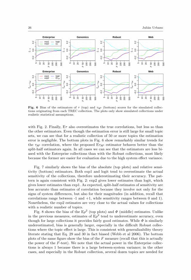
26 Julian Urbano

5 10 20 50 100

200

500

−0.

20.

00.

2

Enterprise

nt

τ−τ

exp1exp2

logitEτ

5 10 20 50 100

200

500

−0.

20.

00.

2

Genomics

nt

τ−τ

5 10 20 50 100

200

500

−0.

20.

00.

2

Robust

nt

τ−τ

5 10 20 50 100

200

500

−0.

20.

00.

2

Web

nt

τ−τ

5 10 20 50 100

200

500

−0.

20.

00.

2

Enterprise

nt

τ AP

−τ A

P

exp1exp2

logitEτAP

5 10 20 50 100

200

500

−0.

20.

00.

2

Genomics

nt

τ AP

−τ A

P

5 10 20 50 100

200

500

−0.

20.

00.

2

Robust

nt

τ AP

−τ A

P

5 10 20 50 100

200

500

−0.

20.

00.

2

Web

nt

τ AP

−τ A

P

Fig. 6 Bias of the estimators of τ (top) and τAP (bottom) scores for the simulated collec-tions originating from each TREC collection. The plots only show simulated collections underrealistic statistical assumptions.

with Fig. 2. Finally, Eτ also overestimates the true correlations, but less so thanthe other estimators. Even though the estimation error is still large for small topicsets, we can see that for a realistic collection of 50 or more topics the estimationerror is negligible. The bottom plots in Fig. 6 show remarkably similar trends forthe τAP correlation, where the proposed EτAP estimator behaves better than thesplit-half estimators again. In all cases we can see that the estimators are less bi-ased with the Enterprise collections than with the Robust collections, most likelybecause the former are easier for evaluation due to the high system effect variance.

Fig. 7 similarly shows the bias of the absolute (top plots) and relative sensi-tivity (bottom) estimators. Both exp1 and logit tend to overestimate the actualsensitivity of the collections, therefore underestimating their accuracy. The pat-tern is again consistent with Fig. 2: exp2 gives lower estimates than logit, whichgives lower estimates than exp1. As expected, split-half estimates of sensitivity areless accurate than estimates of correlation because they involve not only for thesigns of system differences, but also for their magnitudes (in addition, recall thatcorrelations range between -1 and +1, while sensitivity ranges between 0 and 1).Nonetheless, the exp2 estimates are very close to the actual values for collectionswith a realistic number of topics.

Fig. 8 shows the bias of the Eρ2 (top plots) and Φ (middle) estimates. Unlikein the previous measures, estimates of Eρ2 tend to underestimate accuracy, eventhough for large collections it provides fairly good estimates. While Φ is similarlyunderestimated, bias is generally larger, especially in the difficult Robust collec-tions where the topic effect is large. This is consistent with generalizability theoryliterate stating that Eq. 29 and 30 in fact biased (Webb et al 2006). The bottomplots of the same figure show the bias of the F measure (recall that this is actuallythe power of the F -test). We note that the actual power in the Enterprise collec-tions is always 1 because there is a large between-system variance; in the othercases, and especially in the Robust collection, several dozen topics are needed for


5 10 20 50 100

200

500−

0.05

0.05

0.15

0.25

Enterprise

nt

sens

abs

−se

nsab

s exp1exp2logit

5 10 20 50 100

200

500−

0.05

0.05

0.15

0.25

Genomics

nt

sens

abs

−se

nsab

s

5 10 20 50 100

200

500−

0.05

0.05

0.15

0.25

Robust

nt

sens

abs

−se

nsab

s

5 10 20 50 100

200

500−

0.05

0.05

0.15

0.25

Web

nt

sens

abs

−se

nsab

s

5 10 20 50 100

200

500−

0.05

0.05

0.15

0.25

Enterprise

nt

sens

rel−

sens

rel

exp1exp2logit

5 10 20 50 100

200

500−

0.05

0.05

0.15

0.25

Genomics

nt

sens

rel−

sens

rel

5 10 20 50 100

200

500−

0.05

0.05

0.15

0.25

Robust

nt

sens

rel−

sens

rel

5 10 20 50 100

200

500−

0.05

0.05

0.15

0.25

Web

nt

sens

rel−

sens

rel

Fig. 7 Bias of the estimators of sensabs (top) and sensrel (bottom) scores for the simulatedcollections originating from each TREC collection. The plots only show simulated collectionsunder realistic statistical assumptions.

the F -tests to come up significant. We can see that the F1 estimator has a veryclear bias, highly underestimating the accuracy of test collections. As a result, itsuggests the use of many more topics than actually needed to achieve a certainlevel of power in the F -test. This behavior is consistent with our comments inSect. 4.2. In particular, it evidences that the use of the F1 effect size can be mis-leading. It is defined from a minimum detectable difference δmin between the bestand worst systems, and the power analysis tells us how many topics we need todetect that difference. However, if the true difference between the best and worstsystems is larger than δmin to begin with, as is in our collections, the accuracy ofthe collection is systematically underestimated.

6.2 Robustness to Statistical Assumptions

The previous section showed the bias of the estimators in the arguably most re-alistic scenario of non-normal distributions, heteroscedasticity, correlated effectsand random sampling. We now study their robustness to these statistical assump-tions, taking the full set of 83,200 simulated collections. In particular, for eachestimator we run again a variance decomposition analysis over the distributionof estimation errors, thus showing how much of the variability in the estimationerror is attributable to each assumption, the topic set size, and the original TRECcollection. This allows us to detect effects that influence the estimation errors.

Table 3 shows the variance components for the τ and τAP measures. In thecase of the split-half estimators, we see that the largest non-residual effect is thetopic set size, confirming our previous observation that estimates with a handfulof topics are very unstable to begin with. On the other hand, our proposed Eτand EτAP estimators are significantly more robust to the topic set size, meaningthat they can generally be trusted even for small collections. They are also morerobust in general, as shown by the smaller total error variance. This means that

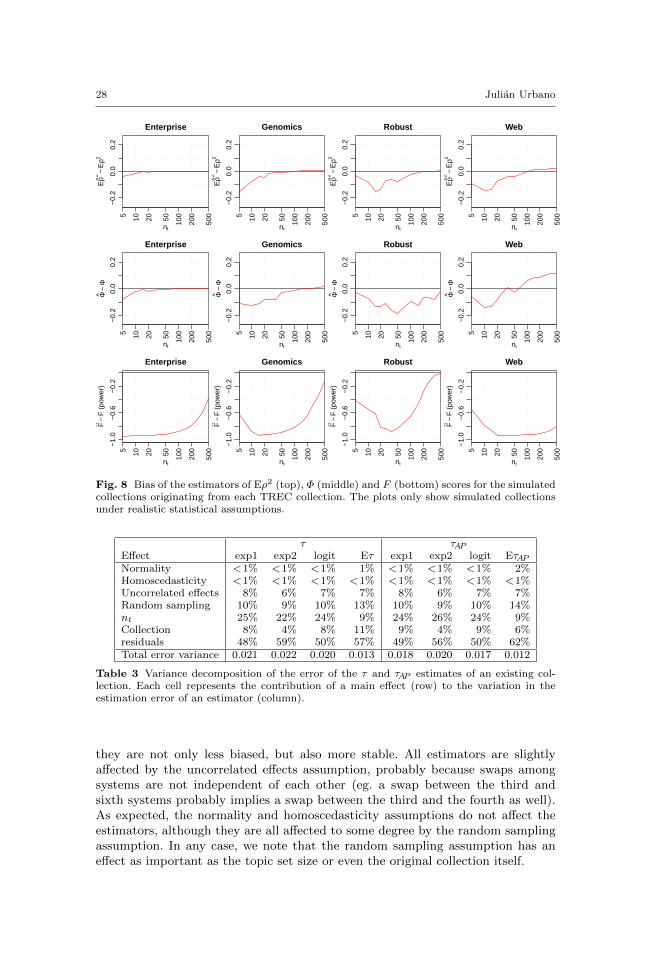
28 Julian Urbano

5 10 20 50 100

200

500

−0.

20.

00.

2

Enterprise

nt

Eρ2

−E

ρ2

5 10 20 50 100

200

500

−0.

20.

00.

2

Genomics

nt

Eρ2

−E

ρ2

5 10 20 50 100

200

500

−0.

20.

00.

2

Robust

nt

Eρ2

−E

ρ2

5 10 20 50 100

200

500

−0.

20.

00.

2

Web

nt

Eρ2

−E

ρ2

5 10 20 50 100

200

500

−0.

20.

00.

2

Enterprise

nt

Φ−

Φ

5 10 20 50 100

200

500

−0.

20.

00.

2

Genomics

nt

Φ−

Φ

5 10 20 50 100

200

500

−0.

20.

00.

2

Robust

nt

Φ−

Φ

5 10 20 50 100

200

500

−0.

20.

00.

2

Web

nt

Φ−

Φ

5 10 20 50 100

200

500

−1.

0−

0.6

−0.

2

Enterprise

nt

F−

F (

pow

er)

5 10 20 50 100

200

500

−1.

0−

0.6

−0.

2

Genomics

nt

F−

F (

pow

er)

5 10 20 50 100

200

500

−1.

0−

0.6

−0.

2

Robust

nt

F−

F (

pow

er)

5 10 20 50 100

200

500

−1.

0−

0.6

−0.

2

Web

nt

F−

F (

pow

er)

Fig. 8 Bias of the estimators of Eρ2 (top), Φ (middle) and F (bottom) scores for the simulatedcollections originating from each TREC collection. The plots only show simulated collectionsunder realistic statistical assumptions.

τ τAPEffect exp1 exp2 logit Eτ exp1 exp2 logit EτAPNormality <1% <1% <1% 1% <1% <1% <1% 2%Homoscedasticity <1% <1% <1% <1% <1% <1% <1% <1%Uncorrelated effects 8% 6% 7% 7% 8% 6% 7% 7%Random sampling 10% 9% 10% 13% 10% 9% 10% 14%nt 25% 22% 24% 9% 24% 26% 24% 9%Collection 8% 4% 8% 11% 9% 4% 9% 6%residuals 48% 59% 50% 57% 49% 56% 50% 62%Total error variance 0.021 0.022 0.020 0.013 0.018 0.020 0.017 0.012

Table 3 Variance decomposition of the error of the τ and τAP estimates of an existing col-lection. Each cell represents the contribution of a main effect (row) to the variation in theestimation error of an estimator (column).

they are not only less biased, but also more stable. All estimators are slightlyaffected by the uncorrelated effects assumption, probably because swaps amongsystems are not independent of each other (eg. a swap between the third andsixth systems probably implies a swap between the third and the fourth as well).As expected, the normality and homoscedasticity assumptions do not affect theestimators, although they are all affected to some degree by the random samplingassumption. In any case, we note that the random sampling assumption has aneffect as important as the topic set size or even the original collection itself.


sensabs sensrelEffect exp1 exp2 logit exp1 exp2 logitNormality < 1% < 1% < 1% < 1% 1% 1%Homoscedasticity < 1% < 1% < 1% < 1% < 1% < 1%Uncorrelated effects 5% 5% 2% 9% 9% 5%Random sampling 2% 4% 3% 4% 5% 8%nt 32% 5% 12% 27% 10% 10%Collection 18% 3% < 1% 3% 3% 1%residual 43% 83% 83% 56% 72% 75%Total error variance 0.005 0.002 0.003 0.023 0.018 0.022

Table 4 Variance decomposition of the error of the sensabs and sensrel estimates of anexisting collection. Each cell represents the contribution of a main effect (row) to the variationin the estimation error of an estimator (column).

Effect Eρ2 Φ F1

Normality <1% <1% <1%Homoscedasticity <1% <1% <1%Uncorrelated effects 7% <1% <1%Random sampling 15% 80% <1%nt 5% 5% 35%Collection 3% <1% 24%residuals 70% 15% 40%Total error variance 0.024 0.225 0.104

Table 5 Variance decomposition of the error of Eρ2, Φ and F estimates of an existing col-lection. Each cell represents the contribution of a main effect (row) to the variation in theestimation error of an estimator (column).

Table 4 shows the results of a similar analysis for the sensabs and sensrelmeasures. The first difference we notice is that absolute sensitivity has smallererror variance and is therefore more robust in general. The exp1 estimators arethe most clearly affected by the topic set size, as evidenced in Fig. 7 as well.The uncorrelated effects and random sampling assumptions appear to affect theestimators as well, though most of the observed variability in the estimation errorsfalls under the residual effect, especially for the exp2 and logit estimators. Thenormality and homoscedasticity assumptions do not affect the estimates.

Table 5 similarly shows the results for the Eρ2 and Φ measures. We can seethat both measures are slightly affected by the topic set size, but the largestnon-residual source of variability is the random sampling assumption. Its effectis remarkably large in Φ because, unlike Eρ2 it estimates the topic difficulties,which can vary considerably with non-random samples (see Sect. 5.4). The tablealso lists the results for the F -test measure, showing that its accuracy dependson the collection (actually, on the ratio of system-variance to topic-variance), andcertainly on the number of topics in the collection. As evidenced by Fig. 8, the F1

estimator is quite unreliable. The normality and homoscedasticity assumptions dono affect.

7 Expected Accuracy of a Hypothetical Test Collection (Reliability)

Here we consider the second scenario where an IR researcher has access to anexisting collection with nt topics and wants to estimate the expected accuracy of

30 Julian Urbano

a hypothetical collection with n′t topics from the same universe. This scenario ispresent for instance when deciding whether to spend resources in judging moretopics for an existing collection. In particular, we are interested in how well ourR(X, n′t,µ) estimates of reliability reflect the true reliability of a topic set size n′t.To this end, we compute the bias of our estimates as in Eq. (4). Recall again thatin this study we can compute the true reliability scores because we know the truesystem scores. As before, we first evaluate the bias of the reliability estimates inthe arguably most realistic scenario of non-normal distributions, heteroscedasticity,correlated effects and random sampling. After that, we evaluate how robust eachestimator is to these assumptions.

7.1 Bias of the Reliability Estimates

For each measure of accuracy, we take the 100 randomly simulated collections foreach of the 13 topic set sizes nt, but only for the case of non-normal distributions,heteroscedasticity, correlated effects and random sampling. For each of these wecompute the 13 estimates of the reliability of new topic set sizes n′t, and comparethe estimates with the actual accuracy observed with sizes n′t. This is done foreach original collection separately, and then all bias scores are averaged acrossthem. This makes a total of 16,900 datapoints for each original TREC collectionand 67,600 overall for each measure.

Fig. 9 shows the bias of the estimates of τ (top plots) and τAP (bottom) relia-bility. For simplicity, we only show the estimates from existing collections of nt =5, 10, 20, 50, 100 and 200 topics; the trends are evident from the figures. The firstdifference we can see is that exp2, which showed good behavior to estimate theaccuracy of an existing collection, is very erratic to estimate the expected accu-racy of a new collection. This is because of the observed behavior that exp2 is notconsistent: it underestimates accuracy until a certain number of topics is reached,beyond where it starts overestimating. Since we are now extrapolating to differenttopic set sizes n′t, this behavior becomes problematic. As the number of existingtopics nt increases, the exp1 and logit estimators get closer to the estimates ofaccuracy from the previous section, where nt = n′t (dashed black line). The ex-trapolations to large topic sets are quite good provided that we have about 100topics to begin with, which is hardly ever the case. With smaller existing collec-tions, both exp1 and logit highly underestimate the expected correlations of largecollections. The proposed Eτ and EτAP show significantly better performance. Infact, with as little as nt = 20 initial topics the predictions are very good. Moreimportantly, we can see that the estimators are consistent and, unlike the split-half estimators, they get closer to the true values as the initial number of topicsincreases.

Fig. 10 similarly shows the bias of the absolute (top plots) and relative sensi-tivity (bottom) reliability estimates. The exp2 estimator shows again very erraticbehavior, especially for small target topic set sizes. On the other hand, the logitestimator shows very good performance; with as little as nt = 20 initial topics itprovides close estimates of the reliability of larger collections. In the case of exp1,the convergence is slower; it requires about 50 initial topics for sensabs and about100 for sensrel. Once again, we appreciate that these split-half estimators also


5 10 20 50 100

200

500

−0.

40.

00.

2

τ exp1

n't

R−

R

nt = 5nt = 50

nt = 10nt = 100

n't = ntnt = 20nt = 200

5 10 20 50 100

200

500

−0.

40.

00.

2

τ exp2

n'tR

−R

5 10 20 50 100

200

500

−0.

40.

00.

2

τ logit

n't

R−

R

5 10 20 50 100

200

500

−0.

40.

00.

2

Eτ

n't

R−

R

5 10 20 50 100

200

500

−0.

40.

00.

2

τAP exp1

n't

R−

R

nt = 5nt = 50

nt = 10nt = 100

n't = ntnt = 20nt = 200

5 10 20 50 100

200

500

−0.

40.

00.

2

τAP exp2

n't

R−

R

5 10 20 50 100

200

500

−0.

40.

00.

2

τAP logit

n't

R−

R

5 10 20 50 100

200

500

−0.

40.

00.

2

EτAP

n't

R−

R

Fig. 9 Bias of the estimators of τ (top) and τAP (bottom) of a new collection with n′t topics,given an existing collection with nt topics. The plots only show simulated collections underrealistic statistical assumptions.

5 10 20 50 100

200

500

−0.

20.

00.

20.

4

sensabs exp1

n't

R−

R

nt = 5nt = 50

nt = 10nt = 100

n't = ntnt = 20nt = 200

5 10 20 50 100

200

500

−0.

20.

00.

20.

4

sensabs exp2

n't

R−

R

5 10 20 50 100

200

500

−0.

20.

00.

20.

4

sensabs logit

n't

R−

R

5 10 20 50 100

200

500

−0.

20.

00.

20.

4

sensrel exp1

n't

R−

R

nt = 5nt = 50

nt = 10nt = 100

n't = ntnt = 20nt = 200

5 10 20 50 100

200

500

−0.

20.

00.

20.

4

sensrel exp2

n't

R−

R

5 10 20 50 100

200

500

−0.

20.

00.

20.

4

sensrel logit

n't

R−

R

Fig. 10 Bias of the estimators of sensabs (top) and sensrel (bottom) of a new collection withn′t topics, given an existing collection with nt topics. The plots only show simulated collectionsunder realistic statistical assumptions.

estimate the expected (biased) estimate of accuracy instead of the expected (true)accuracy of a larger collection.

Fig. 11 shows the bias of the Eρ2 and Φ reliability estimates. We can observethat reliability is generally underestimated. Large initial collections provide betterestimates of new collections, but around nt = 20 initial topics seem sufficient tohave good estimates. These results agree with (Urbano et al 2013b), who analyzedthe effect of the initial collection size on the estimates of the required number oftopics to reach a certain level of reliability. As expected by its poor performance

32 Julian Urbano

5 10 20 50 100

200

500

−0.

20.

00.

10.

2

Eρ2

n't

R−

R

nt = 5nt = 50

nt = 10nt = 100

n't = ntnt = 20nt = 200

5 10 20 50 100

200

500

−0.

20.

00.

10.

2

Φ

n't

R−

R

5 10 20 50 100

200

500

−1.

0−

0.6

−0.

2

F1

n't

R−

R

Fig. 11 Bias of the estimators of Eρ2, Φ and F of a new collection with n′t topics, given anexisting collection with nt topics. The plots only show simulated collections under realisticstatistical assumptions.

in the previous section, the F1 estimator consistently underestimates the power ofthe F -test, regardless of the number of topics in the initial collection.

7.2 Robustness to Statistical Assumptions

In the previous section we evaluated the bias of the reliability estimators in thescenario of non-normal distributions, heteroscedasticity, correlated effects and ran-dom sampling. We now study their robustness to these assumptions with the fullset of 83,200 simulated collections. In particular, for each estimator we run a vari-ance decomposition analysis over the distribution of estimation errors, showingwhat fraction of the variability in the estimation error can be attributed to eachassumption, the initial nt and new n′t topic set sizes, and the original TRECcollection. This provides us with a total of 1,081,600 datapoints per measure.

Table 6 shows the results for τ and τAP . We can see that most of the variabil-ity in the split-half estimators is due to the topic set sizes, either through theirmain effects (nt and n′t) or their interaction effect (nt : n′t). This means thatthe estimation error depends highly on the number of topics available or underconsideration. This is again a direct consequence of the split-half method. On theother hand, the proposed Eτ and EτAP are not affected by the size of the newcollection, and evidence only minor dependence on the size of the existing col-lection. Indeed, through the total error variance we can see that their estimatesclearly outperform the split-half estimators. However, we see a large dependenceon the random sampling assumption, and a noticeable dependence on the uncor-related effects assumption. The normality and homoscedasticity assumptions havenegligible effects.

Table 7 shows similar results for the sensitivity measures. A very large part ofthe variability in the estimation errors is attributable again to the topic set sizeeffects, evidencing that the accuracy of these estimators depends very much onthe size of available data and the size we want to extrapolate to.

Table 8 shows that the estimation of the expected Eρ2 is very slightly affectedby the topic set sizes to extrapolate from and to. Recall that this does not meanthat the estimates are good across sizes, but that the estimation error remainsthe same across sizes. It also shows some dependence on the uncorrelated effectsassumption, but most of the variability in the estimation errors is due to therandom sampling assumption. This is where almost 90% of the variability in Φcomes from, evidencing stability problems if this assumption is not guaranteed.


τ τAPEffect exp1 exp2 logit Eτ exp1 exp2 logit EτAPNormality <1% <1% <1% 2% <1% <1% <1% 3%Homoscedasticity <1% <1% <1% <1% <1% <1% <1% <1%Uncorrelated effects 5% 2% 5% 12% 4% <1% 5% 12%Random sampling 7% 5% 8% 22% 7% 4% 8% 23%n′t 2% 11% 3% <1% <1% 13% 2% <1%nt 18% 1% 14% 9% 21% 2% 17% 12%nt : n′t 6% 9% 3% 2% 8% 10% 5% 2%Collection 13% 2% 14% 15% 14% 2% 14% 8%residuals 48% 70% 52% 37% 46% 68% 51% 40%Total error variance 0.029 0.044 0.027 0.008 0.026 0.048 0.024 0.007

Table 6 Variance decomposition of the estimation error of the expected τ and τAP of a newcollection. Each cell represents the contribution of a main effect (row) to the variation in theestimation error of an estimator (column).

sensabs sensrelEffect exp1 exp2 logit exp1 exp2 logitNormality <1% <1% <1% 2% 3% 4%Homoscedasticity <1% <1% <1% <1% <1% <1%Uncorrelated effects 2% 4% 3% 4% 4% 4%Random sampling 1% 3% 4% <1% <1% 1%n′t 18% 3% 35% 3% 2% 7%nt 6% <1% 1% 12% 1% <1%nt : n′t 21% 30% 4% 11% 5% 2%Collection 14% 2% 8% 2% 1% 1%residuals 38% 57% 44% 65% 83% 81%Total error variance 0.009 0.003 0.002 0.052 0.038 0.036

Table 7 Variance decomposition of the estimation error of the expected sensabs and sensrelof a new collection. Each cell represents the contribution of a main effect (row) to the variationin the estimation error of an estimator (column).

Effect Eρ2 Φ F1

Normality <1% <1% <1%Homoscedasticity <1% <1% <1%Uncorrelated effects 7% <1% <1%Random sampling 19% 86% <1%n′t 3% 4% 46%nt 2% <1% <1%nt : n′t <1% <1% <1%Collection 4% <1% 31%residuals 64% 9% 23%Total error variance 0.019 0.210 0.082

Table 8 Variance decomposition of the estimation error of the expected Eρ2, Φ and F of anew collection. Each cell represents the contribution of a main effect (row) to the variation inthe estimation error of an estimator (column).

In the case of the F1 estimator, we can clearly see robustness to assumptions,although the estimation errors are highly dependent on the target topic set sizes.The normality and homoscedasticity assumptions have negligible effects again.

34 Julian Urbano

8 Discussion

In this paper we were able to study for the first time the true behavior of vari-ous estimators of test collection accuracy and reliability. Thanks to the proposedalgorithm of stochastic simulation, we were able to simulate arbitrarily large col-lections where the expected mean system scores are fixed and known upfront. Thisallowed us to quantify the bias of the estimates and their robustness to several sta-tistical assumptions. The results showed that the common estimators used in theliterature are biased. In the particular case of the Kendall τ and τAP correlations,as well as of the measures from generalizability theory, the estimates tend to benegatively biased: they underestimate the similarity between the results of a testcollection and the true system scores. This is an important result that requiresfurther examination, as a number of studies recently suggested that test collec-tions are generally much smaller than they should, such as (Sakai 2014b; Urbanoet al 2013b; Webber et al 2008).

The results evidence the problems of split-half methods to estimate collectionaccuracy. First, the model they internally fit to the observations is usually selectedbased on its goodness of fit to sets of up to nt/2 topics, and not on the grounds oftheoretical arguments. For instance, the three models in Figure 2 seem to providesimilarly good fits of the data in the right plot, but the extrapolations diverge quitesignificantly as the number of topics increases. There is in principle no theoreticalbasis for choosing one or another, but clearly one of them should be better thanthe others. One could even say that, visually, the exp1 and logit models (red andblue) seem to give a better fit, but the results in Sect. 6 and 7 actually show thatit is exp2 (green) the one that is less biased. At the very least, the results confirmthat there is no single model suitable to all measures, and we even find that somemodels perform well for estimating the accuracy of an existing collection, but notto estimate the expected accuracy of a larger collection.

The second problem, already identified for instance by Sanderson and Zobel(2005), is that the split-half observations are not independent. In any given trial,the selection of topics for the second split is restricted by the random selection oftopics for the first split, because there is a limited number of existing data. Theconsequence is that even if the model to fit is correct, it will be fitted to biasedobservations. This distinction is directly accounted for and modeled in statisticaltheory when defining measures like Eρ2. As we mentioned earlier, it correspondsto the expected square of the correlation between the observed scores and thetrue scores, but it also corresponds to the expected value of the correlation (notsquared) between the observed scores in pairs of randomly parallel collections of thesame size (Cronbach et al 1972). The former is the quantity we are really interestedin, and the latter is what split-half estimators actually provide (Allen and Yen1979). We can directly observe this behavior in the estimates of τ in Figure 9. TheEτ and EτAP estimates converge to the actual expected accuracy En′

tA(X′,µ),

but the split-half estimates converge to our estimates En′tA(X′,µ) of accuracy.

Because the extrapolation models are rather arbitrary, and the observations usedto fit them are not really independent, their estimates are the expected (biased)estimate of accuracy and not the expected (true) accuracy. Since Eτ and EτAP areunbiased, they do estimate the expected true accuracy.


In terms of statistical assumptions, we have seen that the normality assumptionhas negligible effect. This can be explained by the fact that even when the raw ef-fectiveness distributions diverge largely from normality, the residual distributionsare approximately normal, as in Figure 1. In addition, we note that effectivenessmeasures are often defined as the sum of some form of utility across the rank-ing of documents, suggesting that the Central Limit Theorem may actually be atplay with sufficiently large evaluation cut-offs. The homoscedasticity assumptionhad a negligible effect as well. However, we must note that the simulation algo-rithm is designed to reproduce the actual residual distributions observed in theoriginal collection, and not some other distributions that maximize the level of het-eroscedasticity. That is, the simulated collections are heteroscedastic to the sameextend that the original collection is so. In practice, the level of heteroscedasticityis not necessarily large, so this assumption did not affect estimates significantly.The levels of divergence from normality and heteroscedasticity are in principleeasy to control in the simulation algorithm, allowing us to simulate some sortof adversarial systems from the point of view of evaluation. Additionally, we canstudy better ways of preserving the dependence structure of the original data. Inthe algorithm proposed here we focused on preserving the correlation matrix, butother aspects may be of interest, especially given that scores are bounded between0 and 1. These are lines of work we intend to pursue.

We also note that there are several other sources of variability taking placein IR evaluation. In this paper we only studied the variability due to topics, butseveral works have shown that variability due to relevance assessors (Voorhees1998; Carterette and Soboroff 2010; Bailey et al 2008), document corpus (Robert-son and Kanoulas 2012; Sanderson et al 2012), effectiveness measures and pooldepth (Buckley and Voorhees 2000; Voorhees 2001; Kekalainen 2005; Sakai 2006;Buckley et al 2007), and even users (Carterette et al 2011), are not negligible. Itis certainly worthwhile to extend the simulation algorithm to incorporate all thesefactors as well. Also, we note that there are other measures besides the ones westudy here, such as the drank distance (Carterette 2009) or variations of the rankcorrelations (Melucci 2007). Similarly, in this paper we focused on the F -test be-cause we were interested in simultaneously comparing a set of systems, but thereare other statistical tests that can be used to compare individual pairs of systems,such as the t-test, Wilcoxon, bootstrap or permutation tests (Hull 1993; Sakai2006; Smucker et al 2007; Urbano et al 2013a), which can be further coupled withmethods to adjust p-values for multiple comparisons (Carterette 2012; Boytsovet al 2013). We leave these lines for further work as well, especially the study,via simulation, of the actual Type I and Type II error rates of various statisticalsignificance tests.

We note that Eτ and EτAP are unbiased provided that the Wij estimates inEq. (35) are unbiased too. However, it is hard to ensure unbiasedness for arbitrarymeasures producing arbitrary distributions. The Central Limit Theorem applies,but it requires a couple dozen topics to work well. In particular, Figures 6 and 9show that the estimates from small available data are biased, probably becauseof the difficulty in estimating the population standard deviation from a smallsample. Even though the estimators behave very well with more than 20 topics,we should study how to compute better estimates of Wij . The estimators can alsobe extended to incorporate thresholds below which two systems are consideredequal, therefore accounting for ties.

36 Julian Urbano

Finally, throughout this paper we have worked exclusively with point estimates,but we should fully consider interval estimates as well. The split-half estimatorscan produce intervals from the model they fit internally, confidence intervals havebeen derived for the measures from generalizability theory, and simple intervalscan be computed for the proposed Eτ and EτAP estimators. Even though most ofthe point estimates are shown to be biased, this bias can probably be corrected inpractice if we use intervals. We leave this line for future work as well.

9 Conclusions

In this paper we discussed the measurement of test collection reliability from theperspective of traditional ad hoc measures and statistical measures as well. Pastresearch on this topic was partially limited because we do not know the true meaneffectiveness of systems, so it is impossible to assess how accurate our measure-ments really are. The best approximation involves split-half methods, but thisapproach is unfortunately limited by the lack of a theoretical basis, and the avail-able data. To overcome this limitation in IR evaluation research, we proposed analgorithm for stochastic simulation of evaluation results. The algorithm simulatesarbitrarily large test collections for the set of systems and universe of topics rep-resented by some previously available test collection, allowing us to fix the truesystem scores upfront and to control what statistical assumptions hold. Throughseveral indicators, we diagnosed how realistic the simulations are and how closethey resemble real TREC evaluation data. The results showed that the simulatedcollections are indeed realistic, opening new opportunities for IR evaluation re-search where it is necessary to know the true effectiveness of systems.

Through large-scale simulation from TREC data, we evaluated the bias ofestimators in a first scenario where we are interested in the accuracy of an existingtest collection. The results showed that ad hoc measures tend to underestimate theactual reliability of collections, especially when the number of topics is rather small.As a consequence, they suggest the use of more topics than actually needed. Onthe other hand, the statistical measures from generalizability theory provide muchbetter estimates, even though for very small collections they tend to underestimatereliability as well. Finally, we saw that the proper definition of target effect sizesis a non-trivial problem when estimating the power of the F -test.

We also evaluated the bias of the measures in a second scenario where we wantto estimate the expected accuracy of a new test collection of arbitrary size basedon the data available from previous collections. The results confirm that the esti-mates depend largely on the amount of data previously available. For instance, theτ and τAP correlations of hypothetical large collections are very underestimatedunless we have about 100 topics already. In fact, there is a very clear correlationbetween the number of topics available from the previous collection, and the biasof the estimates, indicating that predictions of the required number of topics toinclude in a collection under development are highly overestimated. For the gen-eralizability theory measures we found much smaller biases, especially for smallnumbers of topics. In general, with initial collections of about 50 topics we getquite accurate estimates. To overcome the limitations of the split-half extrapola-tion of τ and τAP , we proposed two new estimators, called Eτ and EτAP , based onstatistical principles. The results confirm that they are unbiased and consistent


estimators, behaving much better than the split-half alternatives and at a smallercomputational expense.

Finally, we studied how robust these measures are to violations of statisticalassumptions. In general, we found that all measures are robust to the normalityand homoscedasticity assumptions, because the actual distributions do not departmuch from these assumptions in practice. We found a slight effect of the uncorre-lated effects assumption, especially on the ad hoc measures in the first scenario andthe statistical measures in the second scenario. In terms of random sampling, wefound generally small effects except with the statistical measures. Even though theeffects are smaller than in principle thought, when absolute scores are of interestwe can have very high errors if random sampling is not guaranteed. The split-halfestimation of the ad hoc measures partially alleviates this problem because theyactually involve a form of resampling. In both scenarios, the most important factoris usually the amount of available data.

We created several scripts for the statistical software R to easily simulate newcollections and help researchers analyze the reliability of test collection designs.They can be downloaded from http://github.com/julian-urbano/irj2015-reliability.

Acknowledgements This work was supported by an A4U postdoctoral grant, a Juan dela Cierva postdoctoral fellowship and the Spanish Government (HAR2011-27540). I am verythankful to Monica Marrero, the anonymous reviewers and the editors for their help in makingthis paper. Thanks also to Rafa Nadal for convincing El Gran Guasch to stop shouting “¡LaDecima!”...that was definitely it.

References

Allen MJ, Yen WM (1979) Introduction to Measurement Theory. WadsworthBailey P, Craswell N, Soboroff I, Thomas P, de Vries AP, Yilmaz E (2008) Relevance As-

sessment: Are Judges Exchangeable and Does it Matter? In: International ACM SIGIRConference on Research and Development in Information Retrieval, pp 667–674

Bodoff D, Li P (2007) Test Theory for Assessing IR Test Collections. In: International ACMSIGIR Conference on Research and Development in Information Retrieval, pp 367–374

Boytsov L, Belova A, Westfall P (2013) Deciding on an Adjustment for Multiplicity in IRExperiments. In: International ACM SIGIR Conference on Research and Development inInformation Retrieval, pp 403–412

Brennan RL (2001) Generalizability Theory. SpringerBrennan RL, Kane MT (1977) An Index of Dependability for Mastery Tests. Journal of Edu-

cational Measurement 14(3):277–289Buckley C, Voorhees EM (2000) Evaluating Evaluation Measure Stability. In: International

ACM SIGIR Conference on Research and Development in Information Retrieval, pp 33–34Buckley C, Dimmick D, Soboroff I, Voorhees EM (2007) Bias and the Limits of Pooling for

Large Collections. Journal of Information Retrieval 10(6):491–508Carterette B (2009) On Rank Correlation and the Distance Between Rankings. In: Interna-

tional ACM SIGIR Conference on Research and Development in Information Retrieval,pp 436–443

Carterette B (2012) Multiple Testing in Statistical Analysis of Systems-Based InformationRetrieval Experiments. ACM Transactions on Information Systems 30(1)

Carterette B, Soboroff I (2010) The Effect of Assessor Error on IR System Evaluation. In: Inter-national ACM SIGIR Conference on Research and Development in Information Retrieval,pp 539–546

Carterette B, Pavlu V, Kanoulas E, Aslam JA, Allan J (2009) If I Had a Million Queries. In:European Conference on Information Retrieval, pp 288–300

38 Julian Urbano

Carterette B, Kanoulas E, Yilmaz E (2011) Simulating Simple User Behavior for System Ef-fectiveness Evaluation. In: ACM International Conference on Information and KnowledgeManagement, pp 611–620

Cohen J (1988) Statistical Power Analysis for the Behavioral Sciences. Lawrence ErlbaumCormack GV, Lynam TR (2006) Statistical Precision of Information Retrieval Evaluation.

In: International ACM SIGIR Conference on Research and Development in InformationRetrieval, pp 533–540

Cornfield J, Tukey JW (1956) Average Values of Mean Squares in Factorials. The Annals ofMathematical Statistics 27(4):907–949

Cramer H (1928) On the Composition of Elementary Errors II. Scandinavian Actuarial Journal11(1):141–180

Cronbach LJ, Gleser GC, Nanda H, Rajaratnam N (1972) The Dependability of BehavioralMeasurements: Theory of Generalizability for Scores and Profiles. Wiley & Sons

Hull D (1993) Using Statistical Testing in the Evaluation of Retrieval Experiments. In: Inter-national ACM SIGIR Conference on Research and Development in Information Retrieval,pp 329–338

Joe H (2014) Dependence Modeling with Copulas. CRC PressKekalainen J (2005) Binary and Graded Relevance in IR Evaluations: Comparison of the

Effects on Ranking of IR Systems. Information Processing and Management 41(5):1019–1033

Lin WH, Hauptmann A (2005) Revisiting the Effect of Topic Set Size on Retrieval Error.In: International ACM SIGIR Conference on Research and Development in InformationRetrieval, pp 637–638

Melucci M (2007) On Rank Correlation in Information Retrieval Evaluation. ACM SIGIRForum 41(1):18–33

von Mises R (1931) Wahrscheinlichkeitsrechnung und ihre Anwendungen in der Statistik undtheoretischen Physik

van Rijsbergen CJ (1979) Information Retrieval. ButterworthsRobertson S, Kanoulas E (2012) On Per-Topic Variance in IR Evaluation. In: International

ACM SIGIR Conference on Research and Development in Information Retrieval, pp 891–900

Sakai T (2006) Evaluating Evaluation Metrics Based on the Bootstrap. In: International ACMSIGIR Conference on Research and Development in Information Retrieval, pp 525–532

Sakai T (2007) On the Reliability of Information Retrieval Metrics Based on Graded Relevance.Information Processing and Management 43(2):531–548

Sakai T (2014a) Designing Test Collections for Comparing Many Systems. In: ACM Interna-tional Conference on Information and Knowledge Management, pp 61–70

Sakai T (2014b) Topic Set Size Design with Variance Estimates from Two-Way ANOVA. In:International Workshop on Evaluating Information Access, pp 1–8

Sakai T (2015) Topic Set Size Design. Information Retrieval JournalSakai T, Kando N (2008) On Information Retrieval Metrics Designed for Evaluation with

Incomplete Relevance Assessments. Journal of Information Retrieval 11(5):447–470Sanderson M (2010) Test Collection Based Evaluation of Information Retrieval Systems. Foun-

dations and Trends in Information Retrieval 4(4):247–375Sanderson M, Zobel J (2005) Information Retrieval System Evaluation: Effort, Sensitivity,

and Reliability. In: International ACM SIGIR Conference on Research and Developmentin Information Retrieval, pp 162–169

Sanderson M, Turpin A, Zhang Y, Scholer F (2012) Differences in Effectiveness Across Sub-collections. In: ACM International Conference on Information and Knowledge Manage-ment, pp 1965–1969

Searle SR, Casella G, McCulloch CE (2006) Variance Components. Wiley & SonsSmucker MD, Allan J, Carterette B (2007) A Comparison of Statistical Significance Tests for

Information Retrieval Evaluation. In: ACM International Conference on Information andKnowledge Management, pp 623–632

Smucker MD, Allan J, Carterette B (2009) Agreement Among Statistical Significance Tests forInformation Retrieval Evaluation at Varying Sample Sizes. In: International ACM SIGIRConference on Research and Development in Information Retrieval, pp 630–631

Sparck Jones K (1974) Automatic Indexing. Journal of Documentation 30(4):393–432, DOI10.1108/eb026524


Tague-Sutcliffe J (1992) The Pragmatics of Information Retrieval Experimentation, Revisited.Information Processing and Management 28(4):467–490

Urbano J, Marrero M (2015) How do Gain and Discount Functions Affect the Correlationbetween DCG and User Satisfaction? In: European Conference on Information Retrieval,pp 197–202

Urbano J, Marrero M, Martın D (2013a) A Comparison of the Optimality of Statistical Signifi-cance Tests for Information Retrieval Evaluation. In: International ACM SIGIR Conferenceon Research and Development in Information Retrieval, pp 925–928

Urbano J, Marrero M, Martın D (2013b) On the Measurement of Test Collection Reliability.In: International ACM SIGIR Conference on Research and Development in InformationRetrieval, pp 393–402

Voorhees EM (1998) Variations in Relevance Judgments and the Measurement of RetrievalEffectiveness. In: International ACM SIGIR Conference on Research and Development inInformation Retrieval, pp 315–323

Voorhees EM (2001) Evaluation by Highly Relevant Documents. In: International ACM SIGIRConference on Research and Development in Information Retrieval, pp 74–82

Voorhees EM (2009) Topic Set Size Redux. In: International ACM SIGIR Conference on Re-search and Development in Information Retrieval, pp 806–807

Voorhees EM, Buckley C (2002) The Effect of Topic Set Size on Retrieval Experiment Error.In: International ACM SIGIR Conference on Research and Development in InformationRetrieval, pp 316–323

Webb NM, Shavelson RJ, Haertel EH (2006) Reliability Coefficients and Generalizability The-ory. Handbook of Statistics 26:81–124

Webber W, Moffat A, Zobel J (2008) Statistical Power in Retrieval Experimentation. In: ACMInternational Conference on Information and Knowledge Management, pp 571–580

Yilmaz E, Aslam JA, Robertson S (2008) A New Rank Correlation Coefficient for InformationRetrieval. In: International ACM SIGIR Conference on Research and Development inInformation Retrieval, pp 587–594

Zobel J (1998) How Reliable are the Results of Large-Scale Information Retrieval Experiments?In: International ACM SIGIR Conference on Research and Development in InformationRetrieval, pp 307–314