Universidad de Castilla La Mancha TESIS DOCTORAL Three essays on computational finance and credit risk measurement and management Autor: Rub´ en Garc´ ıa C´ espedes Director: Manuel Moreno Fuentes Facultad de Ciencias Jur´ ıdicas y Sociales Departamento de An´alisis Econ´ omico y Finanzas Toledo 2014

Welcome message from author
This document is posted to help you gain knowledge. Please leave a comment to let me know what you think about it! Share it to your friends and learn new things together.
Transcript

Universidad de Castilla La Mancha
TESIS DOCTORAL
Three essays on computational finance andcredit risk measurement and management
Autor:
Ruben Garcıa Cespedes
Director:
Manuel Moreno Fuentes
Facultad de Ciencias Jurıdicas y Sociales
Departamento de Analisis Economico y Finanzas
Toledo 2014

To my family and friends
I

Contents
Acknowledgements V
Resumen VI
Summary X
List of Figures XIV
List of Tables XVI
1 Estimating the distribution of total default losses on the Span-
ish financial system 11.1 Introduction . . . . . . . . . . . . . . . . . . . . . . . . . . . . . . . . . . . . . . . . . 1
1.2 The Vasicek (1987) Model . . . . . . . . . . . . . . . . . . . . . . . . . . . . . . . . . 3
1.3 Importance sampling for credit risk . . . . . . . . . . . . . . . . . . . . . . . . . . . . 5
1.3.1 Optimal conditional distribution . . . . . . . . . . . . . . . . . . . . . . . . . 6
1.3.2 Optimal macroeconomic distribution . . . . . . . . . . . . . . . . . . . . . . . 8
1.4 Portfolio data . . . . . . . . . . . . . . . . . . . . . . . . . . . . . . . . . . . . . . . . 8
1.4.1 Probability of default (PD) . . . . . . . . . . . . . . . . . . . . . . . . . . . . 9
1.4.2 Exposure at default (EAD) . . . . . . . . . . . . . . . . . . . . . . . . . . . . 9
1.4.3 Loss given default (LGD) . . . . . . . . . . . . . . . . . . . . . . . . . . . . . 10
1.4.4 Factor correlation (α) . . . . . . . . . . . . . . . . . . . . . . . . . . . . . . . 11
1.4.5 Portfolio expected loss and Basel loss distribution . . . . . . . . . . . . . . . 11
1.5 Importance sampling results . . . . . . . . . . . . . . . . . . . . . . . . . . . . . . . . 12
1.6 Importance sampling modifications and extensions . . . . . . . . . . . . . . . . . . . 13
1.6.1 Random loss given default . . . . . . . . . . . . . . . . . . . . . . . . . . . . . 14
1.6.2 Market mode . . . . . . . . . . . . . . . . . . . . . . . . . . . . . . . . . . . . 18
1.7 Parameter variability . . . . . . . . . . . . . . . . . . . . . . . . . . . . . . . . . . . . 21
II

1.7.1 Pre-crisis analysis . . . . . . . . . . . . . . . . . . . . . . . . . . . . . . . . . 21
1.7.2 Parameter uncertainty . . . . . . . . . . . . . . . . . . . . . . . . . . . . . . . 22
1.8 Conclusions . . . . . . . . . . . . . . . . . . . . . . . . . . . . . . . . . . . . . . . . . 25
Appendix . . . . . . . . . . . . . . . . . . . . . . . . . . . . . . . . . . . . . . . . . . . . . 27
Multimodal distributions . . . . . . . . . . . . . . . . . . . . . . . . . . . . . . . . . . 27
Loop decoupling . . . . . . . . . . . . . . . . . . . . . . . . . . . . . . . . . . . . . . 28
Appendix of Tables . . . . . . . . . . . . . . . . . . . . . . . . . . . . . . . . . . . . . . . . 31
Appendix of Figures . . . . . . . . . . . . . . . . . . . . . . . . . . . . . . . . . . . . . . . 36
2 Extended saddlepoint methods for credit risk measurement 452.1 Introduction . . . . . . . . . . . . . . . . . . . . . . . . . . . . . . . . . . . . . . . . . 45
2.2 Saddlepoint methods . . . . . . . . . . . . . . . . . . . . . . . . . . . . . . . . . . . . 46
2.2.1 Density approximations . . . . . . . . . . . . . . . . . . . . . . . . . . . . . . 46
2.2.2 Cumulative distribution approximations . . . . . . . . . . . . . . . . . . . . . 47
2.3 Credit risk and saddlepoint approximation . . . . . . . . . . . . . . . . . . . . . . . . 49
2.3.1 Saddlepoint method for credit risk . . . . . . . . . . . . . . . . . . . . . . . . 49
2.3.2 Risk contributions . . . . . . . . . . . . . . . . . . . . . . . . . . . . . . . . . 51
2.3.3 Random LGD models . . . . . . . . . . . . . . . . . . . . . . . . . . . . . . . 55
2.3.4 Market mode models . . . . . . . . . . . . . . . . . . . . . . . . . . . . . . . . 57
2.4 Empirical analysis . . . . . . . . . . . . . . . . . . . . . . . . . . . . . . . . . . . . . 58
2.4.1 Data . . . . . . . . . . . . . . . . . . . . . . . . . . . . . . . . . . . . . . . . . 59
2.4.2 Results . . . . . . . . . . . . . . . . . . . . . . . . . . . . . . . . . . . . . . . 59
2.5 Conclusions . . . . . . . . . . . . . . . . . . . . . . . . . . . . . . . . . . . . . . . . . 65
Appendix of Tables . . . . . . . . . . . . . . . . . . . . . . . . . . . . . . . . . . . . . . . . 68
Appendix of Figures . . . . . . . . . . . . . . . . . . . . . . . . . . . . . . . . . . . . . . . 71
3 Taylor expansion based methods to measure credit risk 783.1 Introduction . . . . . . . . . . . . . . . . . . . . . . . . . . . . . . . . . . . . . . . . . 78
3.2 The Vasicek (1987) model . . . . . . . . . . . . . . . . . . . . . . . . . . . . . . . . . 79
3.3 The Pykhtin (2004) approximate model . . . . . . . . . . . . . . . . . . . . . . . . . 80
3.4 Portfolio Results . . . . . . . . . . . . . . . . . . . . . . . . . . . . . . . . . . . . . . 84
3.4.1 Portfolio VaR and ES . . . . . . . . . . . . . . . . . . . . . . . . . . . . . . . 85
3.4.2 Analytical VaR Contributions . . . . . . . . . . . . . . . . . . . . . . . . . . . 85
3.5 Correlated random LGD . . . . . . . . . . . . . . . . . . . . . . . . . . . . . . . . . . 88
3.5.1 Simple random LGD model . . . . . . . . . . . . . . . . . . . . . . . . . . . . 88
III

3.5.2 Advanced random LGD model . . . . . . . . . . . . . . . . . . . . . . . . . . 89
3.6 Conclusions . . . . . . . . . . . . . . . . . . . . . . . . . . . . . . . . . . . . . . . . . 93
Appendix of Figures . . . . . . . . . . . . . . . . . . . . . . . . . . . . . . . . . . . . . . . 94
Conclusions 98
Conclusiones 100
References 102
IV

Acknowledgements
This dissertation is the conclusion of many years of hard work. I have had the privilege to meet
some wonderful and interesting people during these years.
First and foremost, I would like to mention my gratitude to my supervisor Manuel Moreno
Fuentes. Over the past years he has guided me over the process to write this dissertation and helped
me with it. Without his motivation and support this thesis could not have been completed. Being
the advisor of a part-time PhD student can be a risky bet and I want to thank him for giving me
the opportunity to work with him.
The first ideas for this dissertation took place during the AFI - Quantitative Finance Executive
Master, I want to thank Jose Luis Fernandez and Paul MacManus, teachers at AFI, for their support
on the first stages of this dissertation and Juan Antonio de Juan for suggesting the initial topic.
What started as a game finished becoming a PhD dissertation.
I would like to thank professor Paul Glasserman, we met on the Financial Engineering Sum-
mer School 2012 and his suggestions and comments on the importance sampling chapter were ex-
tremely useful. The saddlepoint chapter also got very interesting comments from Cornelis Oosterlee,
Xinzheng Huang and Richard Martin, I am very grateful to them for their suggestions.
I am also indebted to the attendants to the Spanish Finance Forun 2013 for their comments, and
specially to Pedro Serrano and Alberto Bueno-Guerrero.
My family, “ama”, Juan Carlos and Marilo, and friends have always been there supporting me, I
am very grateful to all of them, without their support this dissertation would not had been possible.
Thank you!
V
Resumen
El riesgo de credito es el tipo de riesgo mas relevante al que se enfrentan las entidades financieras
puesto que los riesgos de mercado u operacional son generalmente menos relevantes para este tipo
de empresas. De hecho, durante la crisis financiera anterior el riesgo de credito fue la principal
fuente de perdidas en la cuenta de resultados de las entidades financieras. En este sentido, tanto los
reguladores como las instituciones financieras estan interesados en medir con precision el riesgo de
credito de una cartera. Sin embargo, el problema al que se enfrentan los reguladores es diferente de
aquel al que se enfrentan las instituciones financieras puesto que los primeros estan interesados en
la distribucion de perdidas de todo el sistema financiero en lugar de en la de una cartera concreta.
Los reguladores financieros miden de manera separada los riesgos de credito, de mercado y
operacional y exigen a las instituciones financieras que tengan un nivel de recursos propios suficiente
para soportar escenarios extremos de perdidas con muy baja probabilidad de ocurrencia. Esto se
conoce como la regulacion de Basilea que trata de asegurar la estabilidad del sistema financiero. En
el caso del riesgo de credito el escenario seleccionado tiene una probabilidad de ocurrencia del 0.1%.
Vasicek (1987) propuso el modelo para la medicion del riesgo de credito mas extendido en la
actualidad. Este modelo es utilizado tanto por los reguladores como por la industria bancaria para
obtener la distribucion de perdidas de una cartera. El supuesto fundamental de este modelo es que
el comportamiento de incumplimiento de un cliente j viene determinado por un conjunto de factores
macroeconomicos Z = z1, · · · , zk y un termino idiosincratico εj . El valor de los activos, Vj , de un
cliente se expresa como
Vj =k∑
f=1
αf,jzf + εj
√√√√1−k∑
f=1
α2f,j
El incumplimiento se produce si el valor de los activos cae por debajo de un determinado nivel kj .
En este modelo todos los clientes de la cartera comparten los mismo factores macroeconomicos pero
distintos terminos idiosincraticos. Por tanto, los factores macroeconomicos capturan la interrelacion
entre los clientes. Las perdidas totales de una cartera formada por M clientes se pueden expresar
VI

como
L =
M∑j=1
EADjLGDj1(Vj ≤ kj)
donde EADj es la exposicion en el momento del incumplimiento y LGDj es la tasa de perdida
provocada por el incumplimiento, es decir, 1 menos la tasa de recuperacion final. Bajo condiciones
muy restrictivas el modelo de Vasicek (1987) proporciona una solucion analıtica para la distribucion
de perdidas. Este es el caso de carteras expuestas a un unico factor macroeconomico y formadas por
muchos clientes identicos, esto se conoce como una cartera asintotica con un unico factor de riesgo
(ASRF). Bajo condiciones generales la distribucion de perdidas se suele estimar mediante metodos
de simulacion de Monte Carlo.
Sin embargo la estimacion de escenarios de baja probabilidad empleando metodos de Monte Carlo
puede ser una tarea que requiera mucho tiempo en el caso de carteras grandes y probabilidades de
perdidas muy bajas. Esta estimacion requiere mucho mas tiempo si queremos repartir el riesgo
entre los distintos clientes de la cartera. Como consecuencia, han surgido metodos alternativos al
“simple” Monte Carlo. Estas alternativas se pueden dividir en dos grandes grupos, metodos exactos
y aproximados. El metodo propuesto en Glasserman and Li (2005) se incluye dentro de los metodos
exactos mientras que dos de los metodos aproximados se pueden encontrar en Huang et al. (2007) y
Pykhtin (2004).
En esta tesis exploramos las distintas alternativas para estimar y repartir el riesgo de credito
de una cartera y proponemos nuevos modelos y extensiones para los actualmente disponibles. Con-
trastamos empıricamente la precision de los modelos empleando una cartera formada por todas las
instituciones del sistema financiero espanol. Esta es una cartera muy concentrada en la que todos
los clientes excepto dos (Santander y BBVA) estan expuestos a una unica geografıa. Por lo tanto
esta tesis presenta dos grandes contribuciones a la literatura sobre riesgo de credito:
1. Por un lado exploramos y extendemos algunos de los metodos actualmente disponibles para
medir el riesgo de credito a la vez que proponemos otros nuevos. Mas en detalle, proponemos
considerar un modelo de LGD aleatoria y un modelo de valoracion de mercado para los casos
de muestreo por importancia (IS) y los metodos de saddlepoint. En el caso de los metodos
de saddlepoint adicionalmente proponemos un nuevo metodo para repartir el riesgo que utiliza
polinomios de Hermite. Tambien obtenemos una formula analıtica que permite considerar la
correlacion entre los incumplimientos y las recuperaciones basada en las aproximaciones de
Taylor.
2. Por otro lado, medimos y repartimos el riesgo del sistema financiero espanol. Aunque en
Campos et al. (2007) se trato de medir el riesgo de este sistema financiero, hemos mejorado
su analisis mediante la utilizacion de estimaciones de LGD basadas en datos historicos, hemos
VII

repartido el riesgo entre las distintas instituciones financieras y hemos permitido que las mismas
esten expuestas a mas de un unico factor macroeconomico.
El Capıtulo 1 comienza analizando el modelo propuesto en Glasserman and Li (2005). Primero
introducimos el metodo del muestreo por importancia (IS) y obtenemos los parametros del modelo
para la cartera de instituciones financieras espanolas en Diciembre 2010. Para cada una de las in-
stituciones obtenemos una PD (probabilidad de incumplimiento) basada en su calificacion (rating)
externo, una LGD mediante el procedimiento descrito en Bennet (2002) y los datos historicos de
recuperaciones de la Federal Deposit Insurance Corporation (FDIC), una EAD basada en la infor-
macion publica del balance y, finalmente, la exposicion a los factores macroeconomicos basada en
la informacion publica anual de las instituciones financieras por paıs. A continuacion obtenemos
la distribucion de perdidas de la cartera y el reparto del riesgo basado en los criterios de Value-at-
Risk (VaR) y Expected Shortfall (ES). Encontramos que ambos criterios de reparto pueden generar
resultados muy distintos para las dos instituciones mas grandes.
Seguidamente extendemos el modelo de IS para los casos de recuperaciones aleatorias y valoracion
de mercado. En el caso de recuperaciones aleatorias permitimos que las mismas dependan solo
de factores macroeconomicos o, alternativamente, de factores macroeconomicos e idiosincraticos.
Ambos casos generan resultados similares para la distribucion de perdidas pero no para el reparto del
riesgo. De hecho el modelo mixto de recuperaciones macroeconomicas e idiosincraticas requiere un
numero elevado de simulaciones para generar repartos del riesgo con intervalos de confianza pequenos.
Respecto al modelo de valoraciones de mercado, la distribucion de perdidas se ve considerablemente
desplazada a la derecha ya que ahora existen nuevos estados que producen perdidas elevadas.
Este primer capıtulo finaliza midiendo el impacto de la variabilidad en los parametros del modelo
sobre la distribucion de perdidas. Primero medimos el efecto del ciclo economico obteniendo la
distribucion de perdidas en Diciembre 2007, una fecha anterior a la crisis. De acuerdo a nuestros
resultados la principal fuente de cambios en la distribucion de perdidas son los cambios de ratings. En
segundo lugar, medimos los efectos de la incertidumbre en los parametros calibrados del modelo, αf,j ,
PD y LGD. La incertidumbre en las estimaciones proviene del reducido numero de incumplimientos
disponibles para calibrar dichos parametros. En este caso, de acuerdo a nuestros resultados, la
incertidumbre en la LGD es la principal fuente de preocupacion en la estimacion de la distribucion
de perdidas. Adicionalmente incluimos otras dos extensiones del metodo de IS que desarrollamos,
llamadas “distribuciones multimodales” y “desacople de bucles”.
El Capıtulo 2 estudia el metodo de saddlepoint presentado en Huang et al. (2007) y propone un
nuevo metodo de reparto del riesgo junto con otras extensiones de los metodos de saddlepoint ac-
tualmente disponibles. Primero presentamos los metodos de saddlepoint. Seguidamente proponemos
un nuevo metodo de reparto del riesgo cuya idea principal consiste en no emplear un saddlepoint
VIII

distinto para cada cliente sino emplear el de la cartera total. Mostramos los detalles para modificar
el metodo clasico de aproximacion de saddlepoint. De modo similar al Capıtulo 1, este capıtulo
tambien extiende el modelo de saddlepoint para los casos de LGD aleatoria y valoracion de mercado.
Todas estas extensiones son contrastadas empıricamente empleando la cartera de instituciones
financieras espanolas. El nuevo metodo de reparto propuesto reduce considerablemente el numero
de calculos necesarios para realizar el reparto del riesgo y, comparado con el metodo aproximado
propuesto en Martin and Thompson (2001), este nuevo metodo requiere un tiempo similar de com-
putacion pero los resultados estan mas cercanos a los exactos. Tambien mostramos que los metodos
de saddlepoint no son la mejor opcion bajo recuperaciones mixtas, macroeconomicas e idiosincraticas,
o valoracion de mercado debido al alto numero de calculos necesarios.
Finalmente, en el Capıtulo 3 se aplican las ideas de Pykhtin (2004) sobre aproximaciones basadas
en expansiones de Taylor a nuestro cartera y se propone un nuevo modelo de LGD aleatoria. Comen-
zamos explicando el modelo de Pykhtin (2004) para aproximar la distribucion de perdidas de una
cartera y los criterios de reparto del riesgo basados en VaR y ES presentados en Morone et al. (2012).
Mostramos que los modelos basados en expansiones de Taylor no pueden capturar de manera precisa
el perfil de concentracion de nuestra cartera tanto en la distribucion de perdidas como en el reparto
del riesgo. Este capıtulo finaliza empleando las ideas de la expansion de Taylor para estimar la
distribucion de perdidas de una cartera expuesta a un unico factor que determina el incumplimiento
bajo LGD aleatoria. Este nuevo modelo permite que la LGD tenga un componente idiosincratico y
otro macroeconomico que puede estar correlacionado con el factor macroeconomico que determina el
incumplimiento. Empleando las ideas basadas en la expansion de Taylor y una cartera de referencia
obtenemos resultados muy satisfactorios para los casos de distribucion normal y lognormal en la
LGD y para distintos niveles de correlacion. Creemos que este modelo puede ser implementado de
manera sencilla bajo la regulacion actual de Basilea para considerar las recuperaciones aleatorias
mejor de como lo hace la downturn LGD.
IX

Summary
The credit risk is the most relevant type of risk that financial institutions face as market or oper-
ational risk are usually less relevant for this type of firms. In fact, during the previous financial
crisis credit risk has been the main source of P&L losses. In this sense both financial institutions
and regulators are interested in accurately measuring the credit risk of a given portfolio. However
the problem faced by regulators is different from that faced by financial institutions as they are
concerned about the loss distribution of the whole financial system rather than with that of a given
portfolio.
Financial regulators measure separately the credit, market, and operational risks and force finan-
cial institutions to have a level of own resources so that they can bear extreme scenarios with very
low probability of occurrence. This is known as the Basel regulation and tries to ensure the stability
of the financial system. In the case of the credit risk the target scenario is a 99.9% probability loss
scenario.
Vasicek (1987) proposed the most widely used model to measure credit risk. This model is
used by practitioners and regulators to obtain the loss distribution of a given portfolio. Its main
assumption is that the default behavior of a counterparty j is driven by a set of macroeconomic
factors Z = z1, · · · , zk and an idiosyncratic term εj . The assets value, Vj , of this counterparty is
expressed as
Vj =k∑
f=1
αf,jzf + εj
√√√√1−k∑
f=1
α2f,j
Default happens if the assets value drops below a given threshold level kj . In this model all
the counterparties in the portfolio share the same macroeconomic factors but different idiosyncratic
ones, then the macroeconomic factors capture the interrelation between the counterparties. The
total loss of a portfolio made up of M counterparties can be expressed as
L =
M∑j=1
EADjLGDj1(Vj ≤ kj)
where EADj is the exposure at default and LGDj is one minus the final recovery rate. Under
very restrictive conditions the model in Vasicek (1987) has a closed form representation. This is
X

the case of a single macroeconomic factor and a portfolio made up of many identical counterparties,
this is known as Asymptotic Single Risk Factor (ASRF) portfolio. Under general conditions the loss
distribution is usually estimated through Monte Carlo simulation methods.
However estimating low probability scenarios with simple Monte Carlo methods can be very
time demanding in the case of very low probability losses and big portfolios. This gets even more
time demanding when we want to allocate the risk over the different counterparties in the portfolio.
As a consequence, alternative methods to the pure Monte Carlo one have arisen. We can divide
these alternatives in two broad groups, exact and approximate methods. The method proposed in
Glasserman and Li (2005) is among the exacts methods and two approximate methods can be found
in Huang et al. (2007) and Pykhtin (2004).
In this thesis we explore the different alternatives to estimate and allocate the credit risk of
a portfolio and we propose new models and extensions to the currently available ones. We test
empirically the accuracy of the models considering a portfolio that includes all the institutions in
the Spanish financial system. This is a very concentrated portfolio where all the counterparties but
two of them (Santander and BBVA) are exposed to only one geography. Therefore this thesis has
two broad contributions to the literature:
1. On one hand we explore and extend some of the currently available methods to measure the
credit risk and propose new ones. In more detail, we propose to consider a random LGD model
and a market valuation model for the case of the importance sampling (IS) and the saddle-
point methods. In the case of the saddlepoint we additionally propose a new risk allocation
method that uses Hermite polynomials. We also obtain a closed-form formula that captures
the correlation between default and recoveries based on Taylor expansion approximations.
2. On the other hand, we measure and allocate the risk of the Spanish financial system. Although
Campos et al. (2007) tried to measure the risk of this system, we have improved their anal-
ysis using a historical data based LGD, allocating the risk over the financial institutions and
allowing institutions to be exposed to more than one macroeconomic factor.
Chapter 1 starts analyzing the model proposed in Glasserman and Li (2005). First we introduce
the importance sampling (IS) method and obtain the model parameters for the portfolio of the
Spanish financial system at December 2010. For each institution we obtain a PD based on its external
rating, a LGD based on the Federal Deposit Insurance Corporation (FDIC) historical recovery data
and the procedure described in Bennet (2002), an EAD based on the public balance information, and,
finally, the macroeconomic factor loadings based on the public country by country yearly reports
information of the financial institutions. Then we obtain the loss distribution of the portfolio and the
risk allocation based on the Value-at-Risk (VaR) and the Expected Shortfall (ES) criteria. We find
XI
that both loss allocation criteria can generate very different results for the two biggest institutions.
Next we extend the IS model to work under random recoveries and market valuation. In the case
of the random recoveries we allow for pure macroeconomic recoveries and for mixed idiosyncratic
and macroeconomic recoveries. Both methods produce similar results for the loss distribution but
not for the risk allocation. In fact the mixed idiosyncratic and macroeconomic recoveries model
requires a very high number of simulations to generate risk allocation results with narrow confidence
intervals. Regarding the market valuation model the loss distribution gets considerably shifted to
the right as it allows for new rating states producing high losses.
This first chapter concludes measuring the impact of the variability in the model parameters on
the estimated loss distribution. First we measure the effect of the business cycle obtaining the loss
distribution at December 2007, a pre-crisis date. According to our results the main source of changes
in the loss distribution are changes in the ratings. Secondly, we measure the effects of the uncertainty
in the calibrated model parameters, αf,j , PD, and LGD. The uncertainty in the estimates comes
from the reduced number of historical defaults used to calibrate these parameters. In this case,
according to our results, the LGD uncertainty is the main source of concern in the estimation of the
loss distribution. Additionally we include other two extensions of the IS method that we developed
called, respectively, “multimodal distributions” and “loop decoupling”.
Chapter 2 studies the saddlepoint method introduced in Huang et al. (2007) and proposes a new
risk allocation method and other extensions to the currently available saddlepoint methods. We first
introduce the saddlepoint methods. Later we propose a new risk allocation method whose underlying
idea is based on not using a different saddlepoint for each counterparty in the portfolio but the one of
the whole portfolio. We show the detailed steps to modify the classical saddlepoint approximation.
This chapter also extends the random LGD and market valuation framework exposed in Chapter 1
to work under the saddlepoint approximations.
All these extensions are tested using the portfolio of the Spanish financial system. Our new risk
allocation method reduces considerably the number of calculations required to estimate the risk con-
tributions and, compared with the approximate method presented in Martin and Thompson (2001),
this new method requires a similar computation time but the results are closer to the exact ones.
We also show that the saddlepoint methods are not the best alternative under mixed idiosyncratic
and macroeconomic recoveries or market valuation due to the high number of calculations that are
needed.
Finally, Chapter 3 applies the Taylor expansion based ideas in Pykhtin (2004) to our portfolio and
proposes a new random LGD model. We start explaining the model presented in Pykhtin (2004)
to approximate the loss distribution of a portfolio and the VaR and ES allocation criteria based
on Morone et al. (2012). We show that the Taylor expansion models can not accurately capture
XII

the concentration profile of our portfolio in the loss distribution nor do they in the risk allocation
process. This chapter ends employing the Taylor expansion ideas to estimate the loss distribution of
a portfolio exposed to a single default driving factor under random LGD. This new model allows the
LGD to have an idiosyncratic and a macroeconomic term that may be correlated with the default
driving macroeconomic factor. Using the Taylor expansion based ideas and a benchmark portfolio
we obtain very good results for normal and lognormal LGD models and for different correlation
levels. We consider that this model can be easily implemented under the current Basel regulation
to account for random recoveries better than the downturn LGD does.
XIII

List of Figures
1.1 Assets and deposits share of the top twenty-five Spanish financial institutions. . . . . 36
1.2 Assets, Expected Loss, and Basel 99.9% loss share . . . . . . . . . . . . . . . . . . . 36
1.3 Loss distribution . . . . . . . . . . . . . . . . . . . . . . . . . . . . . . . . . . . . . . 37
1.4 Expected Shortfall (ES) . . . . . . . . . . . . . . . . . . . . . . . . . . . . . . . . . . 37
1.5 Risk Allocation under constant LGD . . . . . . . . . . . . . . . . . . . . . . . . . . . 38
1.6 Comparison of the random LGD and constant LGD loss distributions . . . . . . . . 38
1.7 Risk Allocation under macroeconomic random LGD . . . . . . . . . . . . . . . . . . 39
1.8 Comparison of the two random LGD models and constant LGD . . . . . . . . . . . . 39
1.9 Risk Allocation under mixed macroeconomic and idiosyncratic random LGD . . . . 40
1.10 Median 5Y CDS spread evolution . . . . . . . . . . . . . . . . . . . . . . . . . . . . . 40
1.11 Loss distribution under the market mode . . . . . . . . . . . . . . . . . . . . . . . . 41
1.12 Risk Allocation under market valuation . . . . . . . . . . . . . . . . . . . . . . . . . 41
1.13 Loss distribution of the portfolio at December 2007 . . . . . . . . . . . . . . . . . . . 42
1.14 Loss distribution of the portfolio under the different macroeconomic sensitivity pa-
rameter estimates . . . . . . . . . . . . . . . . . . . . . . . . . . . . . . . . . . . . . . 42
1.15 Loss distribution of the portfolio under PD uncertainty . . . . . . . . . . . . . . . . . 43
1.16 Loss distribution of the portfolio under LGD uncertainty . . . . . . . . . . . . . . . . 43
1.17 Multimodal distributions . . . . . . . . . . . . . . . . . . . . . . . . . . . . . . . . . . 44
2.1 Loss distribution of the Spanish portfolio . . . . . . . . . . . . . . . . . . . . . . . . 71
2.2 Loss distribution of the portfolio under the adaptative saddlepoint approximation . . 71
2.3 Risk Allocation based on 100 simulations . . . . . . . . . . . . . . . . . . . . . . . . 72
2.4 Risk Allocation based on 1000 simulations . . . . . . . . . . . . . . . . . . . . . . . . 72
2.5 Risk Allocation Normal Macroeconomic LGD . . . . . . . . . . . . . . . . . . . . . . 73
2.6 Risk Allocation Lognormal Macroeconomic LGD . . . . . . . . . . . . . . . . . . . . 73
2.7 Risk Allocation Logit Normal Macroeconomic LGD . . . . . . . . . . . . . . . . . . 74
2.8 Risk Allocation Probit Normal Macroeconomic LGD . . . . . . . . . . . . . . . . . . 74
XIV
2.9 Risk Allocation Normal Square Macroeconomic LGD . . . . . . . . . . . . . . . . . . 75
2.10 Risk Allocation Basel Macroeconomic LGD . . . . . . . . . . . . . . . . . . . . . . . 75
2.11 Loss distribution of the Spanish portfolio under market valuation . . . . . . . . . . . 76
2.12 Loss on current value distribution of the Spanish portfolio . . . . . . . . . . . . . . . 76
2.13 VaR and ES contributions for the market mode model . . . . . . . . . . . . . . . . . 77
2.14 VaR and ES contributions on an equally weighted (EAD) portfolio . . . . . . . . . . 77
3.1 Loss distribution and expected shortfall for the Spanish financial institutions . . . . 94
3.2 Risk Allocation for the Spanish financial institutions . . . . . . . . . . . . . . . . . . 95
3.3 Simplified random LGD model . . . . . . . . . . . . . . . . . . . . . . . . . . . . . . 95
3.4 Advanced random LGD model . . . . . . . . . . . . . . . . . . . . . . . . . . . . . . 96
3.5 Advanced random LGD model under Normal LGD . . . . . . . . . . . . . . . . . . . 96
3.6 Advanced random LGD model under Lognormal LGD . . . . . . . . . . . . . . . . . 97
XV

List of Tables
1.1 Spanish financial institutions involved in a merger / acquisition . . . . . . . . . . . . 31
1.2 LGD estimates for losses on deposits and losses on assets . . . . . . . . . . . . . . . 32
1.3 BBVA and Santander country exposures . . . . . . . . . . . . . . . . . . . . . . . . . 32
1.4 Comparison of the 99.9% probability loss levels under different random LGD models 33
1.5 Discount factors by rating grade . . . . . . . . . . . . . . . . . . . . . . . . . . . . . 33
1.6 Average 1-year rating migration matrix . . . . . . . . . . . . . . . . . . . . . . . . . 33
1.7 Comparison of the possible values of α . . . . . . . . . . . . . . . . . . . . . . . . . . 34
1.8 Average S&P default rates . . . . . . . . . . . . . . . . . . . . . . . . . . . . . . . . . 34
1.9 PD uncertainty . . . . . . . . . . . . . . . . . . . . . . . . . . . . . . . . . . . . . . . 35
2.1 Constant conditional LGD models . . . . . . . . . . . . . . . . . . . . . . . . . . . . 68
2.2 Random conditional LGD models . . . . . . . . . . . . . . . . . . . . . . . . . . . . . 68
2.3 Calibrated parameters for the constant conditional LGD model . . . . . . . . . . . . 68
2.4 Tail probabilities for different loss levels for the pure macroeconomic LGD . . . . . . 69
2.5 Calibrated parameters for the random conditional LGD model . . . . . . . . . . . . 69
2.6 Tail probabilities for different loss levels for the mixed macroeconomic and idiosyn-
cratic random LGD . . . . . . . . . . . . . . . . . . . . . . . . . . . . . . . . . . . . 70
2.7 Discount factors by rating grade . . . . . . . . . . . . . . . . . . . . . . . . . . . . . 70
2.8 Average 1-year rating migration matrix . . . . . . . . . . . . . . . . . . . . . . . . . 70
XVI
Chapter 1
Estimating the distribution of total default losses on the Spanish
financial system
1.1 Introduction
This paper quantifies the credit risk loss distribution of the Spanish financial system under a general
Monte Carlo importance sampling (IS) model. One of the main activities in financial institutions
consists on financing investors and paying depositors. Under the Basel regulation the financial
institutions are required to have a minimum level of own resources so that they will not go bankruptcy
in the case that investors do not pay back their loans.
Micro-prudential financial regulation focuses on a one by one supervision of the financial in-
stitutions in order to ensure a maximum default probability of each institution, however a macro-
prudential financial regulation focuses on the whole loss distribution of the financial system. In the
past regulators did just a micro-prudential supervision (see Basel (2006)) however they have recently
switched to a macro-prudential supervision (see Basel (2011)) that tries to capture the interconnect-
edness between the financial institutions, their size and the magnitude of the possible negative effects
in the economy. Over the current economic crisis many financial institutions had to be rescued by
the governments due to their size and potential negative effects in the economy, among others we
have Fannie Mae, Freddie Mac, AIG, Northern Rock, RBS, Lloyds, Nordea, Dexia, ING, Fortis, IKB,
Commerzbank, Hypo Real Estate or Bankia, CAM, CatalunyaCaixa, Novacaixagalicia (NCG), and
Unnim in Spain and some have merged or been absorbed by others financial institutions. Therefore
knowing the loss distribution of a whole financial system and being able to correctly allocate the
risk of each institution is crucial for a good banking supervision and the financial system stability.
This paper estimates the loss distribution of the Spanish financial system under the model
introduced in Vasicek (1987). This model is widely used in practice and is the starting point for
the Basel Internal Rating Based capital charges (see Basel (2006)). As far as we know, Campos et
al. (2007) is the only previous study that tried to measure the risk of the Spanish financial system.
1

However, these authors a) did not take into account the diversification effect of the institutions that
are not only based in Spain, b) used a base recovery value of 60% which, according to USA default
data, is too low, and c) did not allocate the risk over the different financial institutions. Bennet
(2002), Kuritzkes et al. (2002), and Cariboni et al. (2011) used a similar approach to that in Campos
et al. (2007) to define an optimum deposits insurance fund.
As we have said, Campos et al. (2007) considered a unique macroeconomic factor that links all
the institutions in the economy. Our paper goes one step forward as we define as many factors as
countries. We propose to use the public information of consolidated net interest income generated
by the banking groups in the different countries (see BBVA (2009) and Santander (2009)) as a way
to capture the risk exposure of the institutions to the different countries.
We use the Monte Carlo Importance Sampling (IS) technique introduced in Glasserman (2005)
and Glasserman and Li (2005) to measure and allocate the total risk of a certain portfolio. One of
the main advantages of this technique is that it can generate very accurate loss distributions and risk
allocation at a low computational cost compared with that of the standard Monte Carlo method.
In addition, compared with other approximate methods to obtain loss distributions like those in
Pykhtin (2004) and Huang et al. (2007), its accuracy can be improved by increasing the number of
simulations.
To address some criticism raised from the constant recoveries assumption we have used data
of the deposits guarantee fund in United States (FDIC, Federal Deposit Insurance Corporation)
to extend the IS model to deal with random recoveries. After testing several random recoveries
models, our results show that the random recoveries impact on the risk allocation over the different
institutions but not on the portfolio 99.9% probability loss. We have also extended the IS framework
in Glasserman and Li (2005) to obtain the market valuation of the portfolio by using a model similar
to that in Grundke (2009). The impact of this valuation on the loss distribution can double that of
the random recovery model.
This paper provides three major contributions. First, we measure and allocate the risk of the
Spanish financial system under the IS method. Second, we extend the IS method to deal with
more realistic assumptions such as random recoveries and market valuation. Third, we study the
variability of the loss distribution over the business cycle and the variability of the loss distribution
due to the uncertainty in the model inputs. We also highlight that a simple default mode model
can seriously underestimate the possible losses and the risk allocation compared with a market
mode model. We suggest not to focus only in one model but to test the impact of the different
models to asses the solvency of a financial system and the impact of each financial institution. We
believe that our approach goes one step forward in the current risk measurement methods applied by
financial system supervisors and it can be a basic tool to identify Systemically Important Financial
2
Institutions (SIFI) and to quantify the required capital surcharge for these institutions. As stated
in Basel (2011), the Basel banking supervision Committee considers a number of global systemic
banks and sets additional capital requirements using a score function that quantifies the effects of
a default in one of these banks on the whole system. Among other variables, this score function
considers the size, the cross-jurisdictional claims and liabilities, and positions (loans, liabilities) with
other institutions. As we will see later, this interconnectedness among entities is captured in the
Vasicek (1987) model through the macroeconomic common variables.
This paper is organized as follows. Section 2 reviews the main ideas regarding credit risk and the
Vasicek (1987) model. Section 3 introduces the IS model proposed in Glasserman and Li (2005) and
explains the optimal changes in the sampling distributions. Section 4 describes the main features
of the Spanish financial system portfolio. Section 5 presents the IS results, loss distribution, and
risk allocation for this financial system. Section 6 develops the random recoveries and market
mode valuation extensions. Section 7 analyzes the variability of the the loss distribution over the
business cycle and its variability due to the uncertainty in the model parameters estimates. Section
8 summarizes our main results and concludes.
1.2 The Vasicek (1987) Model
Vasicek (1987) introduced the most extended credit risk models assuming that the default behavior of
a given client j (or counterparty) is driven by a set of macroeconomic factors Z = z1, z2, · · · , zk and
an idiosyncratic (client-specific) term εj . The factors ziki=1 and εj are independent and distributed
as standard normal random variables.1 Under these assumptions, default is modeled through the so
called asset value of the client j, defined as
Vj =k∑
f=1
αf,jzf + εj
√√√√1−k∑
f=1
α2f,j (1.1)
This client defaults in her obligations if Vj falls below a given default threshold level k. As
Vj ∼ N(0, 1), we have that k = Φ−1(PDj,C), where Φ(·) denotes the normal distribution function
and PDj,C denotes the historical average default rate of the client j over long enough periods.2
Given the specification (3.1) and conditional to the macroeconomic factors Z, the default prob-
ability of the client j is
Prob(Dj = 1|Z) = Prob(Vj ≤ k|Z) = Φ
Φ−1(PDj,C)−∑k
f=1 αf,jzf√1−
∑kf=1 α
2f,j
1Dependent factors can always be orthogonalized.2It might be more useful to think on the historical average default rates of clients similar to j rather than on the
historical average default rates of the client j.
3

Bank portfolios are composed of this kind of contracts. The total loss of a portfolio including M
contracts or clients is given as L =∑M
j=1 xj , being xj the individual loss of the client or contract
j. Under homogeneous granular portfolios,3 the probability of default Prob(Dj = 1|Z) and the
observed default rates DRz tend to be equal. This means that all the idiosyncratic risk of the
different clients disappear and there is no uncertainty on the loss conditional to the macroeconomic
scenario.
Under granular homogeneous single factor portfolios, the unconditional default rate distribution
function is given as
Prob(DRz ≤ L) = Prob
(Φ
(Φ−1(PDC)− αz√
1− α2
)≤ L
)= Φ
(Φ−1(L)
√1− α2 − Φ−1(PDC)
α
)
Since the Basel II accord, the banking regulation uses the Vasicek (1987) asymptotic single factor
model and forces the financial institutions to have an amount of own resources (equity and other
assets with similar behavior to the equity) equal to the worst loss with a 99.9% probability.
The estimation of the portfolio loss distribution requires estimating PDC for the different portfo-
lios. This can be done by using the historical default rates of the portfolios but another components
are also needed:
1. EAD : Exposure at default, the amount of money owed by the investor when he defaults.
2. LGD : Loss given default, the final loss after all the recovery processes.4
3. α: Sensitivity of the asset value to the macroeconomic factors. The Basel accord provides
standard α values for the different portfolios of a bank.
Then, the portfolio loss can be expressed as
L =
M∑j=1
xj =
M∑j=1
EADjLGDj1(Vj ≤ Φ−1(PDj,C))
In the general case of non-granular, non-homogeneous and multi-factor portfolios, the loss dis-
tribution of a loan portfolio can be obtained by Monte Carlo methods or by approximated ones.
It should be noted that our objective is to know just some statistical measures of the accumulated
loss distribution F (L), being the most important the following ones:
3This type of portfolios is made up of many identical contracts, with the same risk parameters.4For a certain client j, both EADj and LGDj are random variables although they are commonly assumed to be
constant. Along the paper, we will indicate whether the LGD is in percentage terms of the EAD or in euros.
4

1. Value at Risk: V aR(q) = F−1(q).5
2. Expected Shortfall or Tail VaR, that is, the expected loss given that a minimum loss level has
been reached: ES(q) = E(L|L ≥ V aR(q)).
3. Risk contributions of the client j. We can consider two alternatives:
(a) Value at Risk contribution, CV aRj(q) = E(xj |L = V aR(q)).
(b) Expected Shortfall contribution, CESj(q) = E(xj |L ≥ V aR(q)).
1.3 Importance sampling for credit risk
The importance sampling (IS) is a Monte Carlo simulation method that helps to estimate expec-
tations of random variables through an smart change of the sampling distribution. As explained
previously, the most general measure in credit risk is Prob(L ≥ l), directly related to the VaR at a
given confidence level, or the maximum loss with a given probability. Then, to apply the IS method,
we start transforming this probability into an expectation as follows
Prob(L ≥ l) = E(1(L ≥ l)) =
∫ ∞−∞
1(L ≥ l)f(L)dL =
∫ ∞−∞
1(L ≥ l)f(L)
g(L)g(L)dL
One estimator of Prob(L ≥ l) is then given as
P rob(L ≥ l) =1
N
N∑i=1
1(Li ≥ l)f(Li)
g(Li)
where Li is sampled from g(L). As the simulated random variables are independent, the variance
of this estimator is6
V ar(P rob(L ≥ l)) =1
N2
N∑i=1
V ar
(1(Li ≥ l)
f(Li)
g(Li)
)=
1
NV ar
(1(Li ≥ l)
f(Li)
g(Li)
)
≈ 1
N
1
N
N∑i=1
1(Li ≥ l)f2(Li)
g2(Li)−
(1
N
N∑i=1
1(Li ≥ l)f(Li)
g(Li)
)2
where we have used sample statistics. Using this variance estimate and the central limit theorem
we can get the confidence intervals of the probability estimates.
The expected shortfall (ES) is defined as
ES = E(L|L ≥ l) =
∫ ∞−∞
Lf(L|L ≥ l)dL =
∫∞L Lf(L)dL∫∞L f(L)dL
5The Basel regulation requires a bank to have an amount of own resources equal to the V aR(99.9%).6It can be noted that the variance of this estimator vanishes for the sampling distribution g(Li) ∝ 1(Li ≥ l)f(Li).
5

and can be estimated using the IS method as
ES =
∑Ni=1 Li1(Li ≥ l)
f(Li)
g(Li)∑Ni=1 1(Li ≥ l)
f(Li)
g(Li)
The estimators for the VaR and ES risk contributions of the client j are respectively
CV aRj =
∑Ni=1 xj,i1(Li = l)
f(Li)
g(Li)∑Ni=1 1(Li = l)
f(Li)
g(Li)
, CESj =
∑Ni=1 xj,i1(Li ≥ l)
f(Li)
g(Li)∑Ni=1 1(Li ≥ l)
f(Li)
g(Li)
As CV aRj can not be implemented computationally, the following modification is required:
CV aRj =
∑Ni=1 xj,i1(l(1−R) ≤ Li ≤ l(1 +R))
f(Li)
g(Li)∑Ni=1 1(l(1−R) ≤ Li ≤ l(1 +R))
f(Li)
g(Li)
where R is an interval defining parameter. From now on we will employ R = 1%.
The confidence intervals of the expected shortfall and the risk contributions can be derived using
Serfling (1980) to obtain that
V ar(ES) ≈ N
∑Ni=1 (Li − ES)21(Li ≥ l)
(f(Li)g(Li)
)2
(∑Ni=1 1(Li ≥ l)f(Li)
g(Li)
)2 (1.2)
This equation can be extended to provide estimators of the variance of the empirical estimates
of the ES and VaR risk contributions just replacing (Li − ES) by (xj,i − ES) or (xj,i − V aR) and
1(Li ≥ l) by 1(l(1−R) ≤ Li ≤ l(1 +R)) in (1.2).
So far no functional form for the function g(L) has been suggested. Glasserman and Li (2005)
suggested to obtain g(L) in two steps, changing a) the default probabilities conditional on the
macroeconomic factors and b) the macroeconomics factors distribution, respectively.
1.3.1 Optimal conditional distribution
Conditional to the macroeconomic factors realization, the default probability of the client j is
PDj,Z = Φ
Φ−1(PDj,C)−∑k
f=1 αf,jzf√1−
∑kf=1 α
2f,j
Glasserman and Li (2005) suggested to change the default probability by a new one using an
exponential twist
PDj,Z,θ =PDj,Ze
LGDjEADjθ
1 + PDj,Z(eLGDjEADjθ − 1)
6

The change in the default probability of a client depends only on his specific default parameters
plus a parameter θ, common for all the clients. Under this twist, the weight to be assigned to every
loss simulation i of the total portfolio is
W1,i =f(Di,1, · · · , Di,M )
g(Di,1, · · · , Di,M )=
M∏j=1
(PDj,Z
PDj,Z,θ
)Dj,i ( 1− PDi,Z
1− PDj,Z,θ
)1−Dj,i
where Dj,i is the default indicator of the client j in the simulation i. A little algebra leads to
W1,i = e−Liθ+ψ(θ)
where
ψ(θ) =
M∑j=1
ln(
1 + Pj,Z
(eLGDjEADjθ − 1
))(1.3)
Note that, conditional to the macroeconomic state Z, the losses of every client j are independent.
Then, (1.3) implies that ψ(θ) is the cumulant generating function of the random variable L(Z), with
an important role in the saddlepoint approximation method.
Now the problem is to estimate the optimal value of θ that minimizes the variance of the estimator
under the new distribution g(L, θ). Glasserman and Li (2005) proved that
V arg(L,θ)
(1
N
N∑i=1
1(Li ≥ l)W1,i
)≤ e−2θL+2ψ(θ)
Differentiating this upper bound and using the convexity of ψ(θ), the optimum shift θl sat-
isfies ψ′(θl) = l if l > ψ′(0) being null otherwise. Straightforward calculations lead to ψ′(θ) =∑Mj=1 LGDjEADjPDj,Z,θ = Eg(L,θ)(L).
The intuition behind this result is that we aim to obtain high enough losses close to the loss
value l. Under the current macroeconomic factor simulations, expected losses can be much lower
than l and, then, the default probabilities are changed so that the new expected losses equate the
desired loss level, this is done by using θl ≥ 0. However, if the actual expected losses are higher than
the desired one (l), default probabilities are not changed at all. In this case θl should be negative to
get an expected loss of l.
If the VaR based loss contributions (CVaR) are calculated, the default probabilities will always
be shifted to the desired loss level l, so that many simulations will lay inside the interval l(1 ± R).
According to our experience, the number of simulations in the VaR interval can be doubled from
that obtained when forcing θl ≥ 0.
Another interesting property of the Glasserman and Li (2005) approach is that, as ψ(θ) equates
the cumulant generating function, the optimization problem ψ′(θ) = l to be solved under the IS
method coincides with that solved under a saddlepoint approach. The value θl is computed through
7

a non-linear iterative process that departs from an initial estimate obtained by applying a third-order
Taylor expansion to ψ(θ) around θ = 0.7
1.3.2 Optimal macroeconomic distribution
As with the default probability it is possible to change the distribution of the macroeconomic factors
to a new one that reduces the variance of the estimates. The probability we are interested in is
Prob(L ≥ l) =
∫ ∞−∞
Prob(L ≥ l|Z)f(Z)dZ ∝∫ ∞−∞
Prob(L ≥ l|Z)e−Z′Z
2 dZ
The optimal sampling distribution g(Z) is proportional to Prob(L ≥ l|Z)e−(Z′Z)/2. Sampling
from this distribution is complex but feasible through the Markov chain Monte Carlo technique using
the Metropolis-Hasting algorithm. However, Glasserman and Li (2005) suggested sampling from a
normal distribution with the same mode as the optimum distribution, that is, g(Z) ∼ N(µ, I), where
µ = maxZ
Prob(L ≥ l|Z)e−(Z′Z)/2
. According to this, a new weight W2,i = e−µ
′Z+µ′µ/2 has to be
applied and the IS estimators will be given by
P rob(L ≥ l) =1
N
N∑i=1
1(Li ≥ l)W1,iW2,i
E(L|L ≥ l) =1N
∑Ni=1 Li1(Li ≥ l)W1,iW2,i
P rob(L ≥ l)
It still remains to estimate Prob(L ≥ l|Z). To this aim, we decided to use a simple approach
assuming that L|Z ∼ N(a, b2) where8
a = E(L|Z) =
M∑j=1
PDj,ZLGDjEADj
b2 = V ar(L|Z) =M∑j=1
V ar(xj |z) =M∑j=1
PDj,Z(1− PDj,Z)LGD2jEAD
2j
1.4 Portfolio data
We evaluate alternative credit risk measures (loss distribution and risk contributions) considering the
157 financial entities covered by the Spanish deposit guarantee fund (FGD) at December, 2010.9 This
7We used this expansion to approximate the non-linear problem that has to be solved and defined a rule to choose
among the three possible solutions. This approach generated initial estimates very close to the real value of θl.8Other alternatives such as the constant approach or the tail bound approach can be found in Glasserman and Li
(2005).9The FGD is built up to help the financial system stability and includes the three previously existing funds (for
banks, saving banks, and cooperative banks) that were merged in October, 14th, 2011 under the Real Decreto 16/2011.
8
fund was analyzed in Campos et al. (2007) by using a simple single factor model and Monte Carlo
simulations. These authors just tested a range of constant LGDs not directly linked to historical
recovery rates and did not estimate any risk contribution measure. We will try to overcome these
limitations and will assume that the two biggest institutions (BBVA and Santander) are exposed to
other economies and, hence, to other macroeconomic factors.
1.4.1 Probability of default (PD)
We use the credit ratings available at December, 2010 for the Spanish financial institutions and the
historical observed default rates reported by the rating agencies10 to infer a probability of default.
This probability is obtained adjusting an exponential function to the default rates of the ratings up
to B- and imposing a value of 0.3% for a rating AA, a commonly accepted feature. Entities with
no external rating are assigned one notch less than the average rating of the portfolio with external
rating.11 This implies that banks without external rating are assigned a A- rating and the remaining
institutions a BB+ rating, values that are consistent with Campos et al. (2007). Once a rating is
recovered, a long-term default rate is assigned to each institution.
We obtain that the S&P and Moody’s ratings have very similar historical default rates for the
different rating letters while Fitch rating is very different from the other two.12 Even though Fitch
and S&P use the same letters to measure credit risk, the underlying default risk is different, specially
for the very bad ratings. Luckily, no institution had this rating at the date of analysis and, then,
we can still use the calibrated probabilities of default.
1.4.2 Exposure at default (EAD)
Details on assets, liabilities, and deposits for the FGD institutions are available in the AEB, CECA,
and AECR webpages.13 The FGD covers not only depositors but also any loss due to a Governmental
intervention of a financial institution. Hence, our analysis focuses on total assets losses and not only
on losses to depositors.
Balance information at December 2010 was used for the analysis. As many mergers took place
during 2010 (see Table 1.1), we have summed all the information from the different institutions that
belong to the same group.
[INSERT TABLE 1.1 AROUND HERE]
10See S&P (2009), Moody’s (2009), and Fitch (2009).11This average is computed weighting by assets and distinguishing between banks and saving banks.12For the sake of brevity, these results are not reported here and are available upon request.13AEB is the Spanish Bank Association, CECA is the Spanish Saving Bank Association, and AECR is the Spanish
Credit Cooperatives Association. Other sources as Bankscope were tested, however the set of available institutions
was smaller.
9

Figure 1.1 shows the assets and the deposits shares of the top 25 financial institutions. These
entities account for 92.1% of the assets and 92.8% of the deposits in the financial system. The
inverse of the Herfindahl index14 H shows that there are only 10.8 and 13.7 effective counterparties
(from both assets and deposits points of view). This means that the Spanish financial system has
few players and is very concentrated, a common feature in most of the countries worldwide.
[INSERT FIGURE 1.1 AROUND HERE]
1.4.3 Loss given default (LGD)
Schuermann (2004) provided a review of the (academic and practitioner) literature on the LGD. In
more detail, this author focused on the meaning of the LGD and its role in the internal ratings based
(IRB) approach, described the main factors that can drive LGDs, and discussed several approaches
that can be applied to model and estimate the LGD. See also Carey (1998), Altman and Suggitt
(2000), Amihud et al. (2000), Thorburn (2000), Unal et al. (2003), and Altman et al. (2005), among
others, for details on the LGD main characteristics.
As Schuermann (2004) stated in its Section 7, “the factors (or drivers or explanatory variables)
included in any LGD model will likely come from the set of factors we found to be important de-
terminants for explaining the variation in LGD. They include factors such as place in the capital
structure, presence and quality of collateral, industry and timing of the business cycle.” In practice,
industry models such as LossCalcTM use most of these factors, see Gupton and Stein (2002) for
more details on this model.
Bennet (2002) computed the losses due to financial institutions default in the FDIC and showed
that the average losses are bigger in the smallest banks for the period 1986-1998. We update this
analysis for the period 1986-2009 using FDIC public data and the banks assets are updated using the
USA CPI series aiming to have comparable asset sizes. We obtain an average LGD for deposits of
20.73% but this value may be biased as there are many observations in the initial and final years of the
database. Hence, we decide to use E(E(LGDj,t|t)) as an estimate of the real average LGD and obtain
18.35%, that is, 88.56% of the initial average LGD. Then, we estimate E (LGDj,t|Asset Bucket) and
multiply it by the 88.56% adjustment factor. Finally, these LGDs on deposits are transformed into
LGDs on assets using a multiplicative factor of 1.378.15 Table 1.2 provides the LGDs obtained in
this way.
14The Herfindahl index is a measure of portfolio concentration and its inverse can be seen as the number of effective
counterparties in the portfolio. See Allen et al. (2006), Hartmann et al. (2006), and Carbo et al. (2009) for further
details on the Herfindahl index in the banking sector.15This factor is based on the numbers obtained in Bennet and Unal (2011) that used FDIC data for 1986-2007 and
estimated an average depositors LGD of 24.4%, equivalent to a 29.95% total LGD over assets before the time effect
and a 33.61% after the discount effect.
10

[INSERT TABLE 1.2 AROUND HERE]
1.4.4 Factor correlation (α)
We use the total factor sensitivities (α) stated in the Basel accord. These values are computed
according to the formula√
0.12ω + 0.24 (1− ω) where ω = 1−e−50PD
1−e−50 and, hence, range between√
0.12 and√
0.24.16 Recently, the Basel III accord has increased the previous Basel II correlations
by a factor of√
1.25. In this way, we would generate correlations in the range of those used in
Campos et al. (2007). In the following analysis we use the Basel III correlations.
We assume geographic macroeconomic factors and that all the financial institutions are exposed
only to the Spanish factor except for BBVA and Santander that are exposed to additional geogra-
phies. This assumption seems reasonable and its motivation can be seen in Figure 1.1 which shows
that, among the 25 biggest financial institutions, apart from these two entities, only Barclays is not
a fully Spain based bank and its share is very small.
The exposure of BBVA and Santander to the macroeconomic factors is computed using the
reported net interest income by geography obtained from the public 2010 annual reports. We think
that this variable can be a good proxy of the risk faced by a financial institution and, then, it
can indicate appropriately its exposure to the different countries in which the institution operates.
Hence, an income based allocation method can be better than a method only based on exposures
that would assign small weights to the non-Spanish geographies.
Finally, we assume that the correlation between the macroeconomic factors for different countries
is equal to that between the GDP of the countries.17
Table 1.3 shows the exposure of BBVA and Santander to the different countries according to
their net interest incomes. As these country factors are correlated, those exposures have to be
standardized so that the total variance of the sum of each client’s macroeconomic factors equates
one.
[INSERT TABLE 1.3 AROUND HERE]
1.4.5 Portfolio expected loss and Basel loss distribution
The total assets, expected loss, and BIS 99.9% probability loss for the Spanish financial institutions
are 2,921,504 MM e, 453 MM e, and 13,733 MM e, respectively.
Figure 1.2 includes these numbers for the top 25 Spanish financial institutions. The left graph
in this Figure shows the share of these variables for the biggest (ordered by assets) 25 financial
16Kuritzkes et al. (2002) and Campos et al. (2007) use√
0.15 and√
0.30, respectively. In practice, most of the
entities show sensitivities closer to√
0.24.17These correlations are available upon request.
11

institutions. For example, Santander represents 21% of the total assets, 7% of the total BIS 99.9%
loss, and 4% of the expected loss of the Spanish financial system, approximately.
[INSERT FIGURE 1.2 AROUND HERE]
Two conclusions can be extracted from this Figure:
1. Expected loss and Basel 99.9% probability loss generate a very similar ordering.
2. The ordering according to the assets amount is very different from that based on expected or
Basel losses.
The right graph in Figure 1.2 shows the expected loss and Basel 99.9% loss divided by the size
of each institution. We find that the two biggest institutions (BBVA and Santander) share very low
risk parameters.
We will introduce now the results obtained with the IS method as a way to deal with non-
granular and multifactorial portfolios. The main ideas behind this modification of the asymptotic
single factor model are a) BBVA and Santander have some diversification effects as they are exposed
to more than one macroeconomic factor that reduces their risk and b) having non-granular portfolios
increases the risk.
1.5 Importance sampling results
We start orthogonalizing the country factors by applying principal components analysis. As the
correlation between the different economies is very high we end up having a very important common
factor across all the financial institutions. When we obtain the optimum change in the factor mean
for a target loss of 10 times the expected loss we get a 1.62 value in the main common factor and
almost zero otherwise.
Figure 1.3 shows the loss distribution under IS and Monte Carlo simulations. According to
the Basel model the loss level with 99.9% probability is 13,733 MMe. While under multifactorial
non-granular portfolios this loss level is 32,102 MMe, 2.3 times more!18
[INSERT FIGURE 1.3 AROUND HERE]
Figure 1.4 shows the results for the expected shortfall. The VaR contributions are usually less
stable as few simulations fall inside the interval. That is why it is quite common using the expected
shortfall contributions at a loss level whose tail expectation equals the VaR(99.9%) = 32,102 MM
e. In this case this loss level is 16,274 MM e.
18All the figures in the paper are based on the IS results rather than on the Monte Carlo method.
12

[INSERT FIGURE 1.4 AROUND HERE]
Figure 1.5 shows the risk allocation rule according to the ES and VaR contributions and the
confidence intervals for the IS technique.19 These intervals are quite thin after only 10,000 simula-
tions, one of the main advantages of the IS method over the Monte Carlo simulations. Moreover,
the IS method can generate many high loss simulations from a thin loss interval and, then, more
accurate estimates at a lower computation time. The risk picture is completely different from that
obtained using the simple expected loss or the Basel loss model. The main reason for this is that the
non-granularity effect increases (decreases) the risk allocated to the biggest (smallest) institutions.
[INSERT FIGURE 1.5 AROUND HERE]
The main ideas that can be extracted from this Figure are the following:
1. The LGDs (in euros) for BBVA and Santander are higher than the VaR(99.9%). Then their
VaR contributions are zero.
2. The LGD of Bankia is 28,948 MM e, close to the VaR(99.9%) value. Then, this firm copes
most of the risk under the VaR contribution allocation criterion.
3. The risk allocations of Caixabank and Unnim have big confidence intervals. This is due to
the fact that the LGD of both entities together is close to the VaR(99.9%) and there are few
simulations in which Caixabank and Unnim default.
4. The confidence intervals of the 99.9% probability loss ratio are bigger as the risk is adjusted
by the institution size and Unnim has the biggest confidence intervals for the risk allocation.
1.6 Importance sampling modifications and extensions
This Section extends the classical IS framework to deal with random recoveries and market valuation.
Other extensions were performed:20
1. We found that using the mode for the macroeconomic factor shifts may introduce a low sampled
region problem and we developed a method based on the mean of the optimal distribution to
overcome this problem.
2. For granular multifactorial portfolios, we found that the 99.9% probability losses of the Spanish
financial are 13,478 MM e.
19For the VaR contributions we have used a ±1% interval around the desired loss level20For the sake of brevity, we just enumerate here these additional extensions and defer the details to a final Appendix.
13
3. We also evaluated the suitability of the simulation loop decoupling, based on simulating NMacro
macroeconomic scenarios and NDefault default scenarios for each (simulated) macroeconomic
scenario. This modification is very interesting in terms of speed and accuracy for portfolios
with few counterparties that are exposed to the same macroeconomic factor, as it is our case.
The following IS results are based on this extension.
1.6.1 Random loss given default
So far the LGD has been considered as constant but it is a random variable with the same span as
the default rates. Then, it seems natural to assume that the LGD follows a similar distribution to
that of the default rate. Considering this, the simplest case assumes that the whole recovery risk
comes from macroeconomic factors, for example, a single factor called zLGD:
LGDj,Z = Φ
Φ−1(LGDj,C)− αjzLGD√1− α2
j
Under this specification the only parameters to be estimated are αj and the correlation between
zLGD and the rest of the macroeconomic factors. This model also allows to have more macroeconomic
factors but the idea is that no idiosyncratic risk is considered.
The previous formula has been widely studied21 and some of their moments have a closed-form
expression, for example
E(LGDj,Z) = LGDj,C
E(LGD2j,Z) = Φ2
(Φ−1 (LGDj,C) ,Φ−1 (LGDj,C) , α2
j
)where Φ2(x, y, ρ) stands for the probability distribution function (evaluated at the point (x, y))
of a bivariate standard normal random variable with correlation parameter ρ.
We have shown previously that the LGD depends on the institution size and that most of the
defaults in our sample correspond to institutions with less than 1,000 MM e in assets. To keep the
database as clean as possible we will estimate the parameters using just the institutions with this
assets size.
The above formulas and the historical recovery rates from the FDIC data imply LGDj,C =
19.13%, E(LGD2j,Z) = 4.3178% and, therefore, αj = 29.26%. Using these estimates we recover the
zPD and zLGD factors from the historical default series of the FDIC and obtain that the correlation
between the default and recovery factors is 22.63%. The random LGD is introduced replicating the
21See Gordy (2000) or Dullmann et al. (2008).
14

factor correlation of the PD for the LGD as follows:
G =
22.63% 0% · · ·MPD 0% · · · 0%
· · · 0% 22.63%
22.63% 0% · · ·0% · · · 0% MLGD
· · · 22.63%
where MPD = MLGD equates the GDP correlation matrix of the different countries.22 Now not
only PDj,z has to be estimated but also LGDj,z in every simulation step. The optimal exponential
twist and the optimal change in the mean of the macroeconomic factors are obtained using PDj,Z
and LGDj,Z .
Figure 1.6 shows the comparison between the loss distributions of the portfolio under random
and constant LGDs. The 99.9% probability loss is 36,970 MM e, that is, 1.15 times the loss level
under constant LGD. The equivalent expected shortfall level is 19,326 MM e. Figure 1.7 shows the
risk allocation under VaR and ES for the new 99.9% probability loss level. Comparing with Figure
1.5 we can see that this model assigns risk to all the institutions, even to Santander whose initial
LGD was 53,146 MM e, much higher than the 99.9% probability loss. However, as now the LGD is
random, there are some scenarios where Santander defaults and the total loss is close to 36,970 MM
e.
[INSERT FIGURES 1.6 AND 1.7 AROUND HERE]
Compared with the constant LGD case, the random LGD provides the following facts:
1. The confidence intervals in the risk allocation are wider. Now, in the event of default, the
losses have a bigger variability and, hence, the estimation of E(Xi|L = V aR) is also more
volatile.
2. The risk allocations based on the VaR and the ES are relatively “similar” and the risk is not
concentrated in some institutions as in the case of constant LGD.
Under the Basel accord, the random LGD is considered under a very broad definition of a
downturn LGD, defined as the LGD under a stress scenario. This constant downturn LGD tries to
capture somehow the effect of the random LGD.
22For BBVA and Santander the weights of the LGD to the different LGD factors are the same as those defined before
according to their net interest incomes.
15

In the previous setup, two clients with the same LGDj,C and the same sensitivity to the macroe-
conomic variables will have the same LGDj,Z . To avoid this possibility, an idiosyncratic term
γj ∼ N(0, 1) can be included in the previous formula:
LGDj,z,γj = Φ
Φ−1(LGDj,C)− αj(rzLGD + sγj)√1− α2
j
with r2 + s2 = 1. This second specification reduces the correlation between the LGD and the
defaults as a new independent term is considered but it can increase the variability of the recoveries.
The parameter r controls the variability in LGDj,Z over the business cycle. According to our
data, we obtain E(V ar(LGDj,z|z)) = 1.338%,23 implying a variability that is higher than the average
LGDs of the big financial institutions. Intuitively, now, more institutions can generate high and low
loss levels compared to the constant LGD case and the confidence intervals will be wider than under
constant LGD and under fully macroeconomic random LGD. Calibration of the LGD data provides
r = 59.39%
Using these data, for every default and recovery observation in the FDIC database, we recover
the value rzLGD + sγj using the previous formula. Then, for every year, we obtain empirically
E(rzLGD + sγj) that equates rzLGD. In this way we estimate zLGD for every year and obtain that
the correlation between zLGD and the default driving macroeconomic factor zPD is 19.02%.
This new specification causes some changes in the IS framework. For instance, the exponential
twist of the default probabilities conditional to a given set of macroeconomic factors was defined as
that generating an expected loss equal to the target loss level. Now, conditional to these factors,
LGDj,z is not constant and we have two alternatives to find the optimum exponential twist:
1. To keep using the average loss given default LGDj,C regardless of the macroeconomic factors.
2. To estimate E (LGDj,z | z) and E(LGD2
j,z | z)
for every macroeconomic factor simulation.
We use the second method given that E(LGDj,z) has a closed-form expression given as
E(LGDj,z) = Prob(Vj,z < Φ−1(LGDj,C)) = Φ
(Φ−1(LGDj,C)− αrzLGD√
α2(s2 − 1) + 1
)Computing the optimal change in the mean of the factors is a bit more complex as it requires
estimating V ar(LGDj,z|z) or, equivalently, E(LGD2
j,z|z)
, this is,24
E(LGD2
j,z|z)
= Φ2
((Φ−1(LGDj,C)
Φ−1(LGDj,C)
),M,Σ
)23Then, the LGD can change ±11.56% with respect to its mean.24Φ2(X,M,Σ) denotes the probability distribution function (evaluated at the point X) of a bivariate normal random
variable with mean vector M and covariance matrix Σ.
16

with
M =
(αrzLGD
αrzLGD
)
Σ =
(α2s2 + (1− α2) α2s2
α2s2 α2s2 + (1− α2)
)It is worthy to note that the optimal exponential twist is generated using E
(LGDj,Z,γj | Z
)rather
than the simulated LGDj,Z,γj . Then the weightW1,i must be obtained using E(LGDj,Z,γj | Z
)rather
than the realized LGDj,Z,γj , that is, using L∗i =∑M
j=1Dj,iEADjE (LGDj | Z) instead of Li. This is
W1,i = e−L∗i θ+ψ(θ)
where
ψ(θ) =M∑j=1
ln(
1 + Pj,Z
(eE(LGDj,Z,γj |Z)EADjθ − 1
))Figure 1.8 provides the loss distributions under the three possible specifications: constant LGD,
macroeconomic random LGD (LGDC), and macroeconomic plus idiosyncratic random LGD (LGDR).
It can be seen that considering the idiosyncratic term adds some more risk to the 99.9% loss level.
[INSERT FIGURE 1.8 AROUND HERE]
The effect of the idiosyncratic risk is quite small in the loss distribution. Using the IS results,
the 99.9% loss level under the idiosyncratic risk is 37,934 MMe, only 964 MM e more than that
under the macroeconomic LGD model.25 Hence, the impact of the idiosyncratic LGD on the loss
distribution is small compared with that of the macroeconomic LGD. It can also be noted that, for
small (large) loss levels, the idiosyncratic risk term reduces (increases) the chance of those losses.
Regarding the risk allocation, Figure 1.9 shows that, in this case, the (absolute and relative)
risk allocation has even bigger confidence intervals than in the previous models. The reason is that
previously highlighted: given default, the variability of the losses of the client j are wider under the
idiosyncratic LGD model than under the pure macroeconomic LGD.
[INSERT FIGURE 1.9 AROUND HERE]
Other LGD distributions have been tested for the pure macroeconomic LGD model (LGDC) and
the mixed macroeconomic and idiosyncratic LGD model (LGDR).26
Table 1.4 includes the resulting loss distributions using the IS method and shows that the results
of the different random LGD models for the 99.9% loss level are quite similar in all the cases except
for the Log-Normal one.
25The ES equivalent loss is 19,473 MM e.26Detailed results are not reported here and are available upon request.
17

[INSERT TABLE 1.4 AROUND HERE]
To conclude this subsection, we want to mention that, in the random LGD framework, an alter-
native is to apply the IS method to the LGD distribution rather that to the default distribution.27
In fact with the IS ideas we are interested in changing the conditional losses distribution so that
the probability of high losses increases regardless we change the default probabilities or the LGD
distribution. This way of thinking only applies to the case of random conditional LGD. In our case
we have decided to maintain the ideas introduced in the previous sections and change just the default
probabilities.
1.6.2 Market mode
This Subsection evaluates the portfolio risk under a market value model instead of a default mode
one. Under this model the rating of the companies may change over the time and these changes affect
the firm valuation. Then, it is more intuitive to talk about the portfolio value for a given scenario
rather than about portfolio losses. To calibrate a discount factor we obtain the median CDS spread
for a sample of European financial institutions ordered by ratings.28 Figure 1.10 illustrates that
the worse the ratings the higher the CDS spread and that the spread required by the market has
increased considerably since 2008.
[INSERT FIGURE 1.10 AROUND HERE]
We have linearly extended the CDS values for the remaining ratings according to their average
default probability and obtained the daily series of the median CDS spread level for each rating
grade for the period 2008-2011. We assume that this is a representative spread to obtain a discount
factor for the different ratings. However this spread assumes a LGD of 60% for bonds while we
have an average LGD value of 18.35% x 1.378 = 25.28% over assets.29 Hence we adjust linearly the
spread. We assume an average maturity of 3 years for the assets in the portfolio; this is a mixture
of the retail banking assets with longer maturity (like mortgages) and the corporate banking assets
with shorter maturity. The average maturity of the assets is a key assumption in the model, the
greater the maturity the higher the chance of high losses. Unluckily this information is not public
for banks. Table 2.7 reports the 3-year discount factors obtained for each rating in this way.
[INSERT TABLE 2.7 AROUND HERE]
27We acknowledge one of the referees for highlighting this alternative.28These data correspond to 5-year senior CDS since 2008 and were obtained from Markit.29As the financial institutions with available data in Markit have a high level of assets, it is quite possible that the
LGDs of these entities will be smaller than 25.28% but this is a conservative assumption.
18

To simulate the rating transitions, we use an average rating transition matrix over the business
cycle. We adjust the S&P public data in S&P (2010) to take into account the non-rated companies
and we do impose the average probability of default previously adjusted. Table 2.8 includes the
rating transition matrix employed.
[INSERT TABLE 2.8 AROUND HERE]
Migration rule
For a default mode model, the default probability of the client j conditional to a given macroeconomic
scenario is
PDj,Z = Φ
Φ−1(PDj,C)−∑k
f=1 αf,jzf√1−
∑kf=1 α
2f,j
This means that, to simulate the defaults, we can generate a random number Uj ∼ U(0, 1) and
the client defaults if Uj ≤ PDj,Z .
In the case of a market mode model a client can move from an initial rating to a new one.
Let MPj,C,IR,FR denote the average probability (over the cycle) for the client j of migrating
from an initial rating IR to FR, a final one. We can construct the accumulated probabilities
AccumMPj,C,IR,FR.30
Then, for a given macroeconomic state, we can calculate the point in time accumulated proba-
bility of migration between ratings, AccumMPj,Z,IR,FR, as
AccumMPj,Z,IR,FR = Φ
Φ−1(AccumMPj,C,IR,FR)−∑k
f=1 αf,jzf√1−
∑kf=1 α
2f,j
We generate a random number Uj ∼ U(0, 1). Now, if Uj ≤ AccumMPj,Z,IR,D, the new rating of
the client would be D. If AccumMPj,Z,IR,CCC ≤ Uj ≤ MPj,Z,IR,D, the new rating would be CCC
and so on. For each possible final rating state the whole portfolio is evaluated.
Importance sampling
The IS framework must be modified in two ways: a) the exponential twisting rule should be ex-
tended to deal with more than two possible states and b) the conditional portfolio value must be
approximated to estimate the macroeconomic factor mean shift.
Given a macroeconomic scenario Z, the exponential twist of the migration probabilities MP of
the client j from the rating state IR to FR can be extended as follows
MPj,Z,IR,FR,θ =MPj,Z,IR,FRe
Vj,FRθ∑ki=1MPj,Z,IR,ieVj,iθ
30For example, AccumMPj,C,IR,B− = MPj,C,IR,B− +MPj,C,IR,CCC +MPj,C,IR,D.
19

where Vj,i is the loan value to the counterparty j given the rating state i, that is, EADj ×DFiwhere DFi is the discount factor in the state i. Now, the natural extension of the default mode twist
to the case of the mark to market valuation is
Vl =
M∑j=1
k∑h=1
VhMPj,Z,IR,he
Vj,hθ∗∑k
i=1MPj,Z,IR,ieVj,iθ∗
that is, the expected value of the portfolio equates the target value.
We use the normal approximation to change the mean of the factors. Under this approximation,
conditional to the macroeconomic state Z, the portfolio value is distributed as N (µZ , σZ) with
µZ =M∑j=1
k∑h=1
Vj,hMPj,Z,IR,h, σZ =
√√√√ M∑j=1
k∑h=1
V 2j,hMPj,Z,IR,h − (µZ)2
According to the ratings, the market value of the Spanish financial system is 2,842,499 MM e,
representing a 2.7% discount with respect to the total assets. Applying the discounting factors to the
migration probabilities, we get that the expected value of the portfolio is 2,839,535 MM e. Under a
default mode model we focused on 4,528 MM e losses (ten times the expected loss) and, then, the
equivalent market value is equal to 2,842,499 - 4,528 = 2,837,971 MM e. We will use this number
as the target value for the IS method.
We will focus on value losses compared with the current market value rather than with total
assets. The idea is that the difference between total assets and the current market value has been
previously recognized through profit and losses statement and, hence, it does not represent a possible
future loss. It means that debt holders and depositors should be concerned about the possible losses
over the current market value and the amount of own resources that the institution has.
Figure 1.11 shows the loss distribution of the portfolio. For each simulation, losses are obtained
as the market value minus the starting market value, 2,842,499 MM e. The 99.9% probability loss is
68,852 MM e, additional to the current market value loss, equal to 79,006 MM e. As the simulation
speed is very sensitive to the number of possible states, it is very important to use only clearly
different ratings.31
[INSERT FIGURE 1.11 AROUND HERE]
Regarding the VaR and ES based contributions we will allocate the 68,852 MM e loss over
the current market value. Figure 1.12 provides the results and shows that the top contributor is
Santander.
[INSERT FIGURE 1.12 AROUND HERE]
31The analysis has been performed using the rating scale considering modifiers but it could be done without these
modifiers.
20

1.7 Parameter variability
The previous sections have analyzed the credit loss distribution of the Spanish financial system at
December 2010 by considering different credit risk models. We study now the variability of the
main parameters of the Vasicek (1987) model, namely, the EAD, PD, LGD, and the macroeconomic
sensitivity α. We start analyzing the business cycle variability obtaining the loss distribution of the
Spanish financial system at December 2007, a pre-crisis period. Later, we will study the impact of
the variability of the risk parameters on the loss distribution by performing a sensitivity analysis.
1.7.1 Pre-crisis analysis
We estimate the loss distribution at December 2007 to asses the variability of the credit risk measures
over the business cycle. The results can be different from those for December 2010 because of four
possible reasons:
i) The ratings of the financial institutions may be different, therefore their PD may have changed.
ii) Many mergers took place after 2007, therefore the portfolio at December 2007 is more granular.
iii) The amount of assets of the institutions in the portfolio is different, as a consequence their
EAD is different.
iv) As the LGD is assigned using asset buckets and the assets may have changed, the LGD may
have also changed.
In the case of the portfolio at December 2007 the size of the institutions was similar to that
at December 2010. However the ratings changed quite a lot between both dates, being this the
main driver of the change in the loss distribution, followed by the change in the granularity of the
portfolio.
Figure 1.13 includes the loss distribution of the Spanish financial portfolio at December 2007 un-
der the default mode valuation and constant LGD. Compared with the loss distribution at December
2010, the loss distribution is shifted to the left assigning less probability to higher losses. This is
mainly because the ratings deteriorated in the crisis period. In this case the 99.9% probability losses
are only 13,995 MM e, a 44% of the estimate for December 2010. It can also be seen that even
though many mergers had not taken place by December 2007 the loss distribution still has some
discontinuities due to the presence of very big institutions.
[INSERT FIGURE 1.13 AROUND HERE]
21
Regulators should be aware of this kind of risk measurement variability if they want to use this
type of models to quantify the risk of the financial system and to require a financial institution to
have enough capital to make it safe. As suggested in Repullo et al. (2010), one way to deal with
this issue can be to set a variable confidence level for capital requirements so that in periods with
“high” ratings they can focus on more extreme probabilities while they may reduce the confidence
levels in periods with “low” ratings.
1.7.2 Parameter uncertainty
The variability of the risk parameters can be related to the business cycle but also to some uncertainty
in their estimates. The main reason for this uncertainty is that financial institutions do not default
frequently and, then, the estimates of the risk parameters may not be very accurate. In this section
we study the effects of this uncertainty on the loss distribution. Our analysis is based on several
alternatives proposed in the literature for the three most important risk parameters in the default
mode and constant LGD model.
α uncertainty
Our previous results were based on the functional form of the parameter α proposed by the Basel
committee. According to this, αBIS varied between 38% and 54% depending on the PD of the
counterparty. Few studies analyze possible values of α for financial companies. Most of these studies
come from the Moody’s corporation as they have a commercial software32 to implement the Vasicek
(1987) model. Examples of these studies are Lopez (2002), Lee et al. (2009), Qibin et al. (2009),
and Castro (2012).
Lopez (2002) estimated α for general corporations ordered by PD and size buckets while Lee et
al. (2009) estimated this parameter differentiating by financial-industrial sector, PD buckets, and
size buckets. Qibin et al. (2009) obtained quarterly estimates for α and their percentiles considering
several companies grouped by sector (financial vs. industrial) and by geography (Europe-USA).
Finally, Castro (2012) estimated a mean value of α considering three different models. Table 1.7
shows the values of α from these papers and illustrates that the Basel Committee estimates33 are
close or lower than the results in all these papers but for two of the models in Castro (2012).
[INSERT TABLE 1.7 AROUND HERE]
Figure 1.14 reports the loss distributions obtained for the different macroeconomic sensitivity
parameters for the portfolio of Spanish financial institutions at December 2010.
32This software is currently called RiskFrontier and it was previously known as KMV.33These estimates will tend to be closer to 54% rather than to 38% because of the low PD in banks.
22
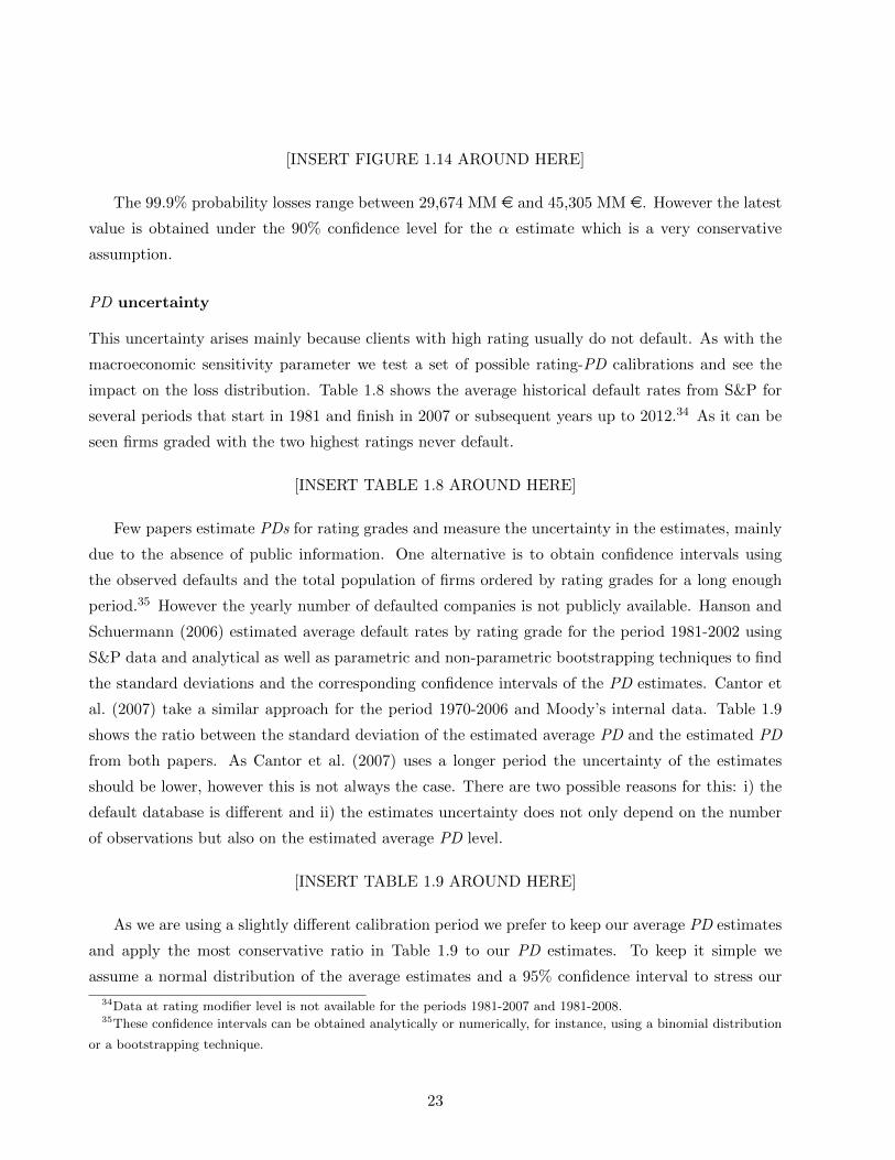
[INSERT FIGURE 1.14 AROUND HERE]
The 99.9% probability losses range between 29,674 MM e and 45,305 MM e. However the latest
value is obtained under the 90% confidence level for the α estimate which is a very conservative
assumption.
PD uncertainty
This uncertainty arises mainly because clients with high rating usually do not default. As with the
macroeconomic sensitivity parameter we test a set of possible rating-PD calibrations and see the
impact on the loss distribution. Table 1.8 shows the average historical default rates from S&P for
several periods that start in 1981 and finish in 2007 or subsequent years up to 2012.34 As it can be
seen firms graded with the two highest ratings never default.
[INSERT TABLE 1.8 AROUND HERE]
Few papers estimate PDs for rating grades and measure the uncertainty in the estimates, mainly
due to the absence of public information. One alternative is to obtain confidence intervals using
the observed defaults and the total population of firms ordered by rating grades for a long enough
period.35 However the yearly number of defaulted companies is not publicly available. Hanson and
Schuermann (2006) estimated average default rates by rating grade for the period 1981-2002 using
S&P data and analytical as well as parametric and non-parametric bootstrapping techniques to find
the standard deviations and the corresponding confidence intervals of the PD estimates. Cantor et
al. (2007) take a similar approach for the period 1970-2006 and Moody’s internal data. Table 1.9
shows the ratio between the standard deviation of the estimated average PD and the estimated PD
from both papers. As Cantor et al. (2007) uses a longer period the uncertainty of the estimates
should be lower, however this is not always the case. There are two possible reasons for this: i) the
default database is different and ii) the estimates uncertainty does not only depend on the number
of observations but also on the estimated average PD level.
[INSERT TABLE 1.9 AROUND HERE]
As we are using a slightly different calibration period we prefer to keep our average PD estimates
and apply the most conservative ratio in Table 1.9 to our PD estimates. To keep it simple we
assume a normal distribution of the average estimates and a 95% confidence interval to stress our
34Data at rating modifier level is not available for the periods 1981-2007 and 1981-2008.35These confidence intervals can be obtained analytically or numerically, for instance, using a binomial distribution
or a bootstrapping technique.
23

PD estimates. This approach imposes that all the estimates must be inside their 95% confidence
interval at the same time. According to this methodology our 95% confidence level for the AAA
estimate is greater than the 95% confidence level for the AA, therefore we bounded the PDs by that
of the next rating. Figure 1.15 reports the loss distribution of the portfolio under this approach.
[INSERT FIGURE 1.15 AROUND HERE]
It can be seen that, under the PD uncertainty and with a 95% confidence level, the 99.9%
probability losses are 36,021 MM e, a 12% higher than the initial estimate.
LGD uncertainty
Regarding estimates of the LGD there is some information about bond LGDs in financial institutions
(see Altman and Kishore (1996)) but few papers estimate the LGD on total assets of defaulted
financial firms. James (1991) provided a first estimate of average losses on assets of 30.51% using
data of US defaulted financial institutions over the period 1985-1988. This number is much higher
than that used by us mainly because a) it is a point-in-time LGD estimate and b) most of the
defaults in the sample were due to small institutions with higher LGD. Therefore shifting the mean
estimates.
More recent papers have focused on the losses for the depositors or the deposits guarantee fund.
Kuritzkes et al. (2002) analyzed the solvency of the FDIC and based their results on the historical
losses suffered by the FDIC estimated in Bennet (2002) for the period 1986-1998. Kaufman (2004)
gets similar results to those in Bennet (2002) but for the period 1980-2002.
Bennet (2002) provided a very detailed analysis of the total losses on total assets and for the
FDIC due to bank failures but they do not perform an analysis by asset buckets. Then we decided to
update the results of Bennet (2002) for losses to depositors and apply the ratio of losses to depositors
to losses on total assets from Bennet and Unal (2011).
Two reasons can explain the statistical uncertainty in the LGDs estimates: i) the ratio of losses
to depositors to losses on total assets may change over the asset buckets36 and ii) the number of
defaults is very low in the highest assets bucket; this may affect the average LGD estimate if the
real LGD is not constant, as it is the case in the observed data. Regarding this issue we can test the
effect of the LGD uncertainty using the 95% confidence level of the estimated LGD.37 Figure 1.16
includes the loss distribution of the portfolio after considering these two sources of uncertainty.
[INSERT FIGURE 1.16 AROUND HERE]
36Table 2 in Bennet and Unal (2011) shows that this ratio can be up to 1.47.37If we have R defaults the LGD estimate is normally distributed with mean µ =
∑Ri=1 LGDi/R and variance∑R
i=1 (LGDi − µ)2/R.
24
Under the LGD uncertainty the 99.9% probability losses are 50,804 MM e with a 95% confidence
level. The effect of the LGD uncertainty is much higher than that of α or PD. This is because the
LGD has a linear impact on the portfolio losses and the uncertainty in the LGD estimates of the
biggest institutions is very high due to the lack of historical defaults.
1.8 Conclusions
This paper has successfully extended the IS framework introduced by Glasserman and Li (2005) to
the case of random recoveries and market mode models. We also tested the extensions of granular
portfolios, simulation loop decoupling, and mean based macroeconomic factors shift.
Considering the LGD as a constant is an assumption that is not supported by the historical
data, therefore this extension allows us to better capture the real behavior of the defaults. A similar
conclusion can be drawn from the market mode valuation: real portfolios can be exposed to mark
to market losses derived from rating changes. The simulation loop decoupling and mean based
macroeconomic factors shift extensions allow for a faster and more accurate risk measurement. The
loop decoupling is very interesting under unifactorial but not granular portfolios as it reduces the
number of calculations required. On the other hand, mean based macroeconomic factors shift enables
a better sampling process and therefore it also reduces the number of simulations required to obtain
narrow confidence intervals of the estimates.
All these extensions allow to use this method inside financial institutions or for regulatory pur-
poses. The extensions and modifications have been tested on a portfolio including Spanish financial
institutions using Monte Carlo simulations as benchmark. Based on Bennet (2002), the LGD of the
different institutions has been obtained and used to estimate the loss distribution of this financial
system.
According to our results the 99.9% probability losses can range between 30,000 and 70,000
MM e depending on the LGD model and the valuation method employed. However, under a
granular portfolio with constant LGD, the 99.9% probability losses would be only 13,478 MM e. The
confidence intervals of the loss distribution obtained using the IS approach are very thin regardless
of the LGD model or the valuation method used.
The confidence intervals of the risk allocation obtained using IS are much thinner than those
obtained with the Monte Carlo method, specially for the VaR based risk allocation. In general,
the risk allocation based on the VaR has wider confidence intervals than that based on the ES.
More precisely, under constant LGD, the VaR based risk allocation has thin confidence intervals
and requires a low number of simulations. However, as we move to a random LGD framework, the
number of simulations required to obtain small confidence intervals in the risk allocation increases
25

considerably. Hence, one possible way to deal with this issue is to use the IS method to estimate the
risk allocation in the case of constant LGD and try to extend other methods such as those in Huang
et al. (2007), Pykhtin (2004) and Voropaev (2011) to deal with the random LGD risk allocation.
Analyzing the suitability of the allocation criteria, we have found that the results can vary
considerably. Probably the best approach is to obtain all the possible results and compare them.
For example, under the CVaR, a given client may have a null risk allocation (as happened with BBVA
and Santander in the constant LGD model) and, hence, provide a infinite risk adjusted return, but
this would lead to a higher concentration.
Finally we have studied the variability of the estimates over the business cycle and the variability
due to the uncertainty in the model parameters estimates. We have shown that the risk estimates
can vary considerably over the business cycle. Regarding the parameters uncertainty we have shown
that currently the main driver of uncertainty in the risk estimates is the LGD. This is due to the
low number of historical defaults for the biggest financial institutions bucket.
This kind of analysis can provide a basic tool for regulators to analyze the solvency of the
financial system and to study the relevance of the financial institutions in the economy. This last
issue is specially interesting to establish the so called systematically important financial institutions
surcharge in BIS III.
26
Appendix
Multimodal distributions
We studied the behavior of the importance sampling algorithm on a symmetric portfolio made up
of clients with the same PDi, LGDi, EADi, and macroeconomic factor sensitivity. These clients
were split in two halves that are sensitive to two different macroeconomic factors. Surprisingly,
we obtained a mode of the optimum sampling distribution that was not symmetric although the
problem was completely symmetric.
To understand this issue, Figure 1.17 provides the function g(Z) = Prob(L ≥ l|Z)e−Z′Z
2 for a
simple case.38 Two modes can clearly be seen. These modes have a direct impact on the estimated
risk and on the risk contributions estimates and generate a bias. The intuition is that using one
of the modes will simulate normal macroeconomic factors with a mean that is very close to zero
for one of the factors and positive for the other one. Then, most of the simulations will generate
large losses on half of the portfolio and almost no losses on the other half. Hence, the importance
sampling algorithm will generate two effects:
• The loss distribution will be underestimated because only half of the portfolio defaults in the
simulations and the estimation confidence intervals will be very big.
• Even though the portfolio is symmetric, the half of the portfolio that does not default on the
simulations will have very low risk contributions.
[INSERT FIGURE 1.17 AROUND HERE]
This bimodal characteristic should generate large confidence intervals for the estimates. However,
this is only the case if the two modes are not close. To our knowledge, this is the first time that this
bias has been detected in the literature.
Glasserman and Li (2005) proposed using the mode of the optimun sampling distribution to
change the mean of the macroeconomic factors because it is easier to be estimated than other
statistical moments as the mean or the median.39 Trying to solve this problem, we decided to
estimate the mean or the median of the optimum distribution g(Z). Reitan and Aas (2010) proposed
estimating the mean using Markov Chain Monte Carlo (MCMC)40 and the Metropolis-Hasting
38We use the normal approximation, 1,000 counterparties, parameters PD=1%, LGD=40%, EAD=1,000, α = 55%,
and target loss equal to 10 times the expected loss.39It is easier to find numerically the maximum of a multivariate distribution than obtaining random samples from
it.40However, they did not highlight any bias related to the use of the mode.
27

algorithm, a very suitable procedure as it does not require having a proper density function that
integrates one as is our case.
However the MCMC method is not very fast and we propose a method based again on importance
sampling to estimate the mean and variance of g(Z). We will sample from a normal distribution
and then use weights to estimate these two moments. In more detail, these estimators are41
µg(Z) =1
N
N∑i=1
ZjcProb(Li > l|Zi)e−ZiZ′i
21
φ(Zi)µ,Ω
σ2g(Z) =
1
N
N∑i=1
Z2i cProb(Li > l|Zi)e−
ZiZ′i
21
φ(Zi)µ,Ω− µ2
g(Z)
where Zi is obtained from a multivariate normal random variable φ(Z)µ,Ω. After many trials,
the best results are obtained when the parameter µ is set to zero and the variance matrix Ω is the
identity one.
The constant c ensures that we are working with a probability distribution, that is,
1 =1
N
N∑i=1
cProb(Li > l|Zi)e−ZiZ′i
21
φ(Zi)µ,Ω
This method is much faster than the MCMC and, at the same time, generates accurate results.
Alternatively to the mean, the median of the optimum g(Z) can also be used. This median is
estimated for every macroeconomic factor of the set Z = z1, · · · , zk. In the case of the component
k, the median is obtained ordering the simulations 1 to N according to the values of zk and then
adding the weight 1N cProb(Li > l|Zi)e−
ZiZ′i
21
φ(Zi)µ,Ωuntil the value 50% is obtained, that is,
mediang(Zi) = min
(zi,n
∣∣∣∣∣ 1
N
n∑i=1
[cProb(Lj > l|Zi)e−
ZiZ′i
21
φ(Zi)µ,σ
]= 50%
)
Loop decoupling
The importance sampling (IS) framework explained in Glasserman and Li (2005) assumed that, for
every macroeconomic factor simulation, an optimal exponential twist is calculated and one default
simulation is performed. However, we can also generate several default simulations for every macroe-
conomic factor simulation. This is interesting when dealing with almost unifactorial portfolios that
are not granular as the number of required optimizations gets reduced.
Let Ne and Ni denote the number of macroeconomic scenarios and default simulations conditional
to a macroeconomic scenario, respectively. Then, N = NeNi. Again the confidence intervals for the
41After all the experiments, the best results where obtained using as variance the maximum between 1 and the
optimum variance.
28

estimations can be estimated as explained before but, now, the defaults are not totally independent
as some of them share macroeconomic scenarios. Hence, the confidence interval formulas must be
slightly modified:
V ar( Prob(L ≥ l)) =1
N2
Ne∑i=1
V ar
(Ni∑k=1
1(Li,k ≥ l)f(Li,k)
g(Li,k)
)
=Ne
N2V ar
(Ni∑k=1
1(Li,k ≥ l)f(Li,k)
g(Li,k)
)
=Ne
N2V ar(Ri) ≈
Ne
N2
1
Ne
Ne∑i=1
R2i −
(1
Ne
Ne∑i=1
Ri
)2
where Li,k stands for the loss on the external simulation i and the internal simulation k.
A similar result can be obtained for the expected shortfall (ES)
Xn1 =1
N
Ne∑i=1
Ni∑k=1
Li,k1(Li,k ≥ l)f(Li,k)
g(Li,k)=
1
N
Ne∑i=1
Si
Xn2 =1
N
Ne∑i=1
Ni∑k=1
1(Li,k ≥ l)f(Li,k)
g(Li,k)=
1
N
Ne∑i=1
Ri
V ar(ES) =V ar(Xn1 − ESXn2)
X2n2
=1N2
∑Nei=1 V ar(Si − ESRi)
X2n2
≈ N
∑Nei=1 (Si − ESRi)2∑Ne
i=1Ri(1.4)
The previous formula can be used to obtain the variance of the risk contributions. The variance
of the expected shortfall contributions of client j can be obtained replacing Si in (1.4) by Si,j
Si,j =
Ni∑k=1
xi,k,j1(Li,k ≥ l)f(Li,k)
g(Li,k)
The variance of the VaR contribution estimates of the client j is obtained changing ES by V aR
in (1.4) and redefining Si and Ri by Si,j and Ri,j , respectively
Si,j =
Ni∑k=1
xi,k,j1(l(1−R) ≤ Li,k ≤ l(1 +R))f(Li,k)
g(Li,k)
Ri,j =
Ni∑k=1
1(l(1−R) ≤ Li,k ≤ l(1 +R))f(Li,k)
g(Li,k)
As it can be seen, the sums of the default simulations for every macroeconomic factor simulation
have to be performed. This forces to keep all the default data for one macroeconomic simulation.
However, this is a tractable problem as, in general, 1, 000 ≤ Ne ≤ 10, 000 and 100 ≤ Ni ≤ 1, 000.
29

In the case of the financial institutions there is a big non-granular effect and, then, it may be
interesting to decouple the simulation loops. In this case we generate the loss distribution using, for
example, 1,000 x 100 simulations. This method generates very accurate results and, at the same
time, is much faster than the general one on the case of very non-granular portfolios as happens in
the Spanish financial system.
30
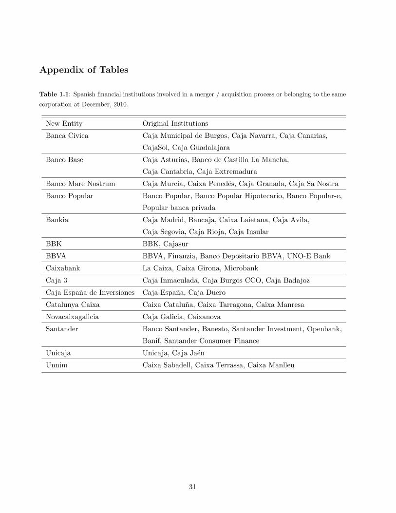
Appendix of Tables
Table 1.1: Spanish financial institutions involved in a merger / acquisition process or belonging to the same
corporation at December, 2010.
New Entity Original Institutions
Banca Civica Caja Municipal de Burgos, Caja Navarra, Caja Canarias,
CajaSol, Caja Guadalajara
Banco Base Caja Asturias, Banco de Castilla La Mancha,
Caja Cantabria, Caja Extremadura
Banco Mare Nostrum Caja Murcia, Caixa Penedes, Caja Granada, Caja Sa Nostra
Banco Popular Banco Popular, Banco Popular Hipotecario, Banco Popular-e,
Popular banca privada
Bankia Caja Madrid, Bancaja, Caixa Laietana, Caja Avila,
Caja Segovia, Caja Rioja, Caja Insular
BBK BBK, Cajasur
BBVA BBVA, Finanzia, Banco Depositario BBVA, UNO-E Bank
Caixabank La Caixa, Caixa Girona, Microbank
Caja 3 Caja Inmaculada, Caja Burgos CCO, Caja Badajoz
Caja Espana de Inversiones Caja Espana, Caja Duero
Catalunya Caixa Caixa Cataluna, Caixa Tarragona, Caixa Manresa
Novacaixagalicia Caja Galicia, Caixanova
Santander Banco Santander, Banesto, Santander Investment, Openbank,
Banif, Santander Consumer Finance
Unicaja Unicaja, Caja Jaen
Unnim Caixa Sabadell, Caixa Terrassa, Caixa Manlleu
31

Table 1.2: LGD estimates for losses on deposits and losses on assets for the period 1986-2009 obtained from
the FDIC public data by institution size.
Assets (in $bn) Count Mean (deposits) Mean (assets)
< 1 1148 18.61% 25.65%
1 - 5 49 15.50% 21.37%
5 - 15 7 9.95% 13.72%
> 15 8 6.39% 8.82%
Table 1.3: BBVA and Santander country exposures obtained according to the net interest income data
published in their 2010 Annual Reports.
Country BBVA Santander
Spain 37.7% 18.8%
Mexico 33.5% 5.9%
United States 9.6% 6.8%
Argentina 2.8% 0%
Chile 4.0% 5.3%
Colombia 4.0% 0%
Peru 4.8% 0%
Venezuela, RB 3.7% 0%
Portugal 0% 2.6%
United Kingdom 0% 14.5%
Brazil 0% 36.8%
Italy 0% 0.7%
Finland 0% 0.8%
Germany 0% 7.5%
Total 100% 100%
32

Table 1.4: Comparison of the 99.9% probability loss levels under different random LGD models. We consider
a pure macroeconomic LGD (LGDC), based on transformations of a random normal macroeconomic variable
zLGD, the random LGD conditional to the macroecomic variable zLGD (LGDR), and the case of LGD|zLGD
with Beta and Gamma distributions.
Model Loss (MM e) Model Loss (MM e)
Normal LGDC 37,160 Probit Normal LGDC 35,999
Normal LGDR 38,131 Probit Normal LGDR 35,318
Lognormal LGDC 29,309 Normal2 LGDC 36,826
Lognormal LGDR 36,139 Normal2 LGDR 36,587
Logit Normal LGDC 35,909 Beta LGDR 37,616
Logit Normal LGDR 34,997 Gamma LGDR 37,578
Table 1.5: Discount factors by rating grade based on the average CDS spread and 3-year average maturity.
Investment Grade
Rating AAA AA+ AA AA- A+ A A- BBB+ BBB BBB-
Discount Factor 98.71% 98.69% 98.6% 98.37% 97.93% 97.14% 96.96% 96.63% 96.02% 95.94%
Speculative Grade
Rating BB+ BB BB- B+ B B- CCC/C
Discount Factor 95.79% 95.51% 94.99% 94.04% 92.33% 89.26% 83.93%
Table 1.6: Average 1-year rating migration matrix from S&P (2010).
AAA AA+ AA AA- A+ A A- BBB+ BBB BBB- BB+ BB BB- B+ B B- CCC D
AAA 91% 4% 3% 1% 0% 0% 0% 0% 0% 0% 0% 0% 0% 0% 0% 0% 0% 0.0249%
AA+ 2% 79% 12% 4% 1% 1% 0% 0% 0% 0% 0% 0% 0% 0% 0% 0% 0% 0.0253%
AA 1% 1% 84% 8% 3% 1% 0% 0% 0% 0% 0% 0% 0% 0% 0% 0% 0% 0.027%
AA- 0% 0% 5% 80% 10% 3% 1% 0% 0% 0% 0% 0% 0% 0% 0% 0% 0% 0.03%
A+ 0% 0% 1% 5% 81% 9% 3% 1% 0% 0% 0% 0% 0% 0% 0% 0% 0% 0.0356%
A 0% 0% 0% 1% 5% 81% 7% 3% 1% 0% 0% 0% 0% 0% 0% 0% 0% 0.0459%
A- 0% 0% 0% 0% 1% 7% 79% 8% 3% 1% 0% 0% 0% 0% 0% 0% 0% 0.0651%
BBB+ 0% 0% 0% 0% 0% 1% 7% 78% 9% 2% 0% 0% 0% 0% 0% 0% 0% 0.1005%
BBB 0% 0% 0% 0% 0% 1% 1% 7% 80% 6% 2% 1% 0% 0% 0% 0% 0% 0.1659%
BBB- 0% 0% 0% 0% 0% 0% 0% 2% 9% 76% 6% 3% 1% 1% 0% 0% 0% 0.2871%
BB+ 0% 0% 0% 0% 0% 0% 0% 1% 2% 13% 69% 7% 4% 1% 1% 0% 1% 0.5112%
BB 0% 0% 0% 0% 0% 0% 0% 0% 1% 3% 9% 71% 9% 3% 2% 1% 1% 0.9257%
BB- 0% 0% 0% 0% 0% 0% 0% 0% 0% 1% 2% 9% 71% 9% 4% 1% 1% 1.6925%
B+ 0% 0% 0% 0% 0% 0% 0% 0% 0% 0% 0% 2% 7% 73% 9% 3% 2% 3.111%
B 0% 0% 0% 0% 0% 0% 0% 0% 0% 0% 0% 0% 2% 9% 66% 9% 7% 5.735%
B- 0% 0% 0% 0% 0% 0% 0% 0% 0% 0% 0% 0% 1% 3% 10% 60% 14% 10.5892%
CCC/C 0% 0% 0% 0% 0% 0% 0% 0% 0% 0% 0% 0% 1% 2% 3% 11% 63% 19.5689%
33
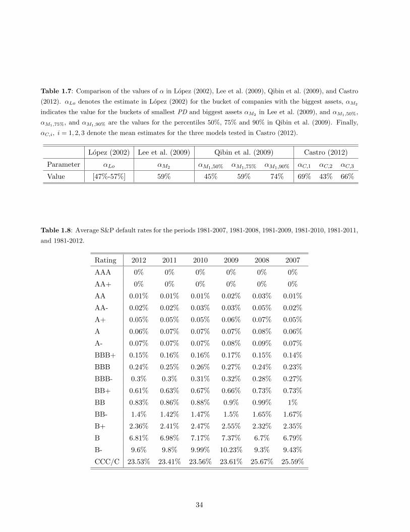
Table 1.7: Comparison of the values of α in Lopez (2002), Lee et al. (2009), Qibin et al. (2009), and Castro
(2012). αLo denotes the estimate in Lopez (2002) for the bucket of companies with the biggest assets, αM2
indicates the value for the buckets of smallest PD and biggest assets αM2 in Lee et al. (2009), and αM1,50%,
αM1,75%, and αM1,90% are the values for the percentiles 50%, 75% and 90% in Qibin et al. (2009). Finally,
αC,i, i = 1, 2, 3 denote the mean estimates for the three models tested in Castro (2012).
Lopez (2002) Lee et al. (2009) Qibin et al. (2009) Castro (2012)
Parameter αLo αM2 αM1,50% αM1,75% αM1,90% αC,1 αC,2 αC,3
Value [47%-57%] 59% 45% 59% 74% 69% 43% 66%
Table 1.8: Average S&P default rates for the periods 1981-2007, 1981-2008, 1981-2009, 1981-2010, 1981-2011,
and 1981-2012.
Rating 2012 2011 2010 2009 2008 2007
AAA 0% 0% 0% 0% 0% 0%
AA+ 0% 0% 0% 0% 0% 0%
AA 0.01% 0.01% 0.01% 0.02% 0.03% 0.01%
AA- 0.02% 0.02% 0.03% 0.03% 0.05% 0.02%
A+ 0.05% 0.05% 0.05% 0.06% 0.07% 0.05%
A 0.06% 0.07% 0.07% 0.07% 0.08% 0.06%
A- 0.07% 0.07% 0.07% 0.08% 0.09% 0.07%
BBB+ 0.15% 0.16% 0.16% 0.17% 0.15% 0.14%
BBB 0.24% 0.25% 0.26% 0.27% 0.24% 0.23%
BBB- 0.3% 0.3% 0.31% 0.32% 0.28% 0.27%
BB+ 0.61% 0.63% 0.67% 0.66% 0.73% 0.73%
BB 0.83% 0.86% 0.88% 0.9% 0.99% 1%
BB- 1.4% 1.42% 1.47% 1.5% 1.65% 1.67%
B+ 2.36% 2.41% 2.47% 2.55% 2.32% 2.35%
B 6.81% 6.98% 7.17% 7.37% 6.7% 6.79%
B- 9.6% 9.8% 9.99% 10.23% 9.3% 9.43%
CCC/C 23.53% 23.41% 23.56% 23.61% 25.67% 25.59%
34

Table 1.9: Ratio of standard deviation of the PD estimate and the PD estimate.
Rating Cantor et al. (2007) Schuermann (2004)
AAA - -
AA 71.19% 62.78%
A 38.27% 23.12%
BBB 14.24% 23.52%
BB 6.64% 9.87%
B 3.51% 4.37%
CCC 3.84% 4.36%
35

Appendix of Figures
0
5
10
15
20
Assets Share
%
SANTANDER
BBVA
BANKIA
LA C
AIXA
POPULAR
SABADELL
CATALUNYACAIX
ANCG
BANCA CIV
ICACAM
MARE N
OST.
BANKINTER, S
ABASE
CAJA E
SPAÑABBK
IBERCAJA
UNICAJA
BARCLAYS
BANCO PASTOR
UNIMM
CAJAM
AR
BANCO DE V
ALENCIA
CAJA L
ABORAL
KUTXA
CAJA 3
Total share: 0.92145
1/H: 10.8308
0
2
4
6
8
10
12
14
16
Deposits Share
%
SANTANDER
BBVA
BANKIA
LA C
AIXA
POPULAR
MARE N
OST.
BANCA CIV
ICA
SABADELLNCG
CAM
CATALUNYACAIX
A
BASE
CAJA E
SPAÑABBK
BANKINTER, S
A
IBERCAJA
UNICAJA
UNIMM
CAJAM
AR
BARCLAYS
CAJA L
ABORAL
CAJA 3
KUTXA
BANCO PASTOR
BANCO DE V
ALENCIA
Total share: 0.92808
1/H: 13.6687
Figure 1.1: Assets and deposits share of the top twenty-five Spanish financial institutions.
0
5
10
15
20
25
%
Total Assets, Expected Loss and BIS Loss(99.9%) share
SANTANDER
BBVA
BANKIA
LA C
AIXA
POPULAR
SABADELL
CATALUNYACAIX
ANCG
BANCA CIV
ICACAM
MARE N
OST.
BANKINTER, S
ABASE
CAJA E
SPAÑABBK
IBERCAJA
UNICAJA
BARCLAYS
BANCO PASTOR
UNIMM
CAJAM
AR
BANCO DE V
ALENCIA
CAJA L
ABORAL
KUTXA
CAJA 3
Assets: 0.92145Expected Loss: 0.64632BIS Loss(99.9%): 0.75048
0
0.01
0.02
0.03
0.04
0.05
0.06
0.07
0.08
0.09
0.1
Exp
ecte
d Lo
ss (
%)
Expected Loss (%) and BIS Loss (%)
Expected LossBIS Loss(99.9%)
0
0.2
0.4
0.6
0.8
1
1.2
1.4
1.6
1.8
2
BIS
Los
s (%
)
SANTANDER
BBVA
BANKIA
LA C
AIXA
POPULAR
SABADELL
CATALUNYACAIX
ANCG
BANCA CIV
ICACAM
MARE N
OST.
BANKINTER, S
ABASE
CAJA E
SPAÑABBK
IBERCAJA
UNICAJA
BARCLAYS
BANCO PASTOR
UNIMM
CAJAM
AR
BANCO DE V
ALENCIA
CAJA L
ABORAL
KUTXA
CAJA 3
Figure 1.2: Assets, Expected Loss, and Basel 99.9% loss share of the top 25 Spanish financial institutions.
Left and right graphs show, respectively, the amount allocation and the allocated amount relative to the
institution size.
36

0 1 2 3 4 5 6 7 8
x 104
10−6
10−5
10−4
10−3
10−2
10−1
100
Loss Distribution
IS 10,000MC 1,000,000
2.2 2.4 2.6 2.8 3 3.2 3.4 3.6 3.8 4
x 104
10−3
Loss Distribution
IS 10,000MC 1,000,000
Figure 1.3: Loss distribution using 10,000 importance sampling (IS) and 1,000,000 Monte Carlo (MC)
simulations. The black and red lines show, respectively, the Monte Carlo and IS results while the blue lines
indicate the 5%-95% confidence interval of the IS estimates. Left and right graphs show, respectively, the tail
distribution and its detail in the neighborhood of the 99.9% probability loss level.
0 0.5 1 1.5 2 2.5 3 3.5 4 4.5 5
x 104
0
0.5
1
1.5
2
2.5
3
3.5
4
4.5
5x 10
4 Expected Shortfall
1.2 1.4 1.6 1.8 2 2.2
x 104
2.6
2.8
3
3.2
3.4
3.6
3.8
x 104 Expected Shortfall
Figure 1.4: Expected Shortfall (ES) using 10,000 importance sampling (IS) simulations. The red and blue
lines show, respectively, the IS results for the expected shortfall estimate and its 5%-95% confidence intervals.
37

0
20
40
60
80
100
%
Loss (99.9%) Allocation
SANTANDER
BBVA
BANKIA
LA C
AIXA
POPULAR
SABADELL
CATALUNYACAIX
ANCG
BANCA CIV
ICACAM
MARE N
OST.
BANKINTER, S
ABASE
CAJA E
SPAÑABBK
IBERCAJA
UNICAJA
BARCLAYS
BANCO PASTOR
UNIMM
CAJAM
AR
BANCO DE V
ALENCIA
CAJA L
ABORAL
KUTXA
CAJA 3
ELBIS Loss(99.9%)IS CVaRIS CESMC CVaRMC CES
0
2
4
6
8
10
12
%
Loss (99.9%) ratio (%)
SANTANDER
BBVA
BANKIA
LA C
AIXA
POPULAR
SABADELL
CATALUNYACAIX
ANCG
BANCA CIV
ICACAM
MARE N
OST.
BANKINTER, S
ABASE
CAJA E
SPAÑABBK
IBERCAJA
UNICAJA
BARCLAYS
BANCO PASTOR
UNIMM
CAJAM
AR
BANCO DE V
ALENCIA
CAJA L
ABORAL
KUTXA
CAJA 3
BIS Loss(99.9%)IS CVaRIS CESMC CVaRMC CES
Figure 1.5: Risk allocation under constant LGD based on expected loss (EL), Basel loss 99.9% (BIS),
contributions to VaR (CVaR) and ES (CES) both using importance sampling (IS) and Monte Carlo (MC)
criteria. Left and right graphs show, respectively, the total risk allocation and the allocated risk relative to
the institution size.
0 1 2 3 4 5 6 7 8
x 104
10−6
10−5
10−4
10−3
10−2
10−1
100
Loss Distribution
IS 10,000 x 100 Const LGDMC 1,000,000 Const LGDIS 10,000 x 100 Rnd LGDMC 1,000,000 Rnd LGD
2.9 3 3.1 3.2 3.3 3.4 3.5 3.6 3.7 3.8
x 104
10−3
Loss Distribution
IS 10,000 x 100 Const LGDMC 1,000,000 Const LGDIS 10,000 x 100 Rnd LGDMC 1,000,000 Rnd LGD
Figure 1.6: Comparison of the random LGD (Rnd LGD) and constant LGD (Const LGD) loss distributions.
Black lines show the results of the Monte Carlo (MC) method using 1,000,000 simulations. The red and blue
lines show, respectively, the importance sampling (IS) estimates and their 5%-95% confidence intervals using
10,000 macroeconomic scenarios and 100 default simulations on each macroeconomic scenario. Left and right
graphs show, respectively, the tail distribution and its detail in the neighborhood of the 99.9% probability
loss level.
38

0
5
10
15
20
25
30
35
40
%
Loss (99.9%) Allocation
SANTANDER
BBVA
BANKIA
LA C
AIXA
POPULAR
SABADELL
CATALUNYACAIX
ANCG
BANCA CIV
ICACAM
MARE N
OST.
BANKINTER, S
ABASE
CAJA E
SPAÑABBK
IBERCAJA
UNICAJA
BARCLAYS
BANCO PASTOR
UNIMM
CAJAM
AR
BANCO DE V
ALENCIA
CAJA L
ABORAL
KUTXA
CAJA 3
IS CVaRIS CES
0
0.5
1
1.5
2
2.5
3
3.5
4
%
Loss (99.9%) ratio (%)
SANTANDER
BBVA
BANKIA
LA C
AIXA
POPULAR
SABADELL
CATALUNYACAIX
ANCG
BANCA CIV
ICACAM
MARE N
OST.
BANKINTER, S
ABASE
CAJA E
SPAÑABBK
IBERCAJA
UNICAJA
BARCLAYS
BANCO PASTOR
UNIMM
CAJAM
AR
BANCO DE V
ALENCIA
CAJA L
ABORAL
KUTXA
CAJA 3
IS CVaRIS CES
Figure 1.7: Risk allocation under macroeconomic random LGD (LGDC) for the VaR (CVaR) and the
ES (CES) criteria. Continuous and dashed lines represent, respectively, the IS estimates and the 5%-95%
confidence intervals. Left and right graphs show, respectively, the total risk allocation and the allocated risk
relative to the institution size.
0 1 2 3 4 5 6 7 8
x 104
10−6
10−5
10−4
10−3
10−2
10−1
100
Loss Distribution
IS 10,000 x 100 Const LGDMC 1,000,000 Const LGDIS 10,000 x 100 Rnd LGD 1MC 1,000,000 Rnd LGD 1IS 10,000 x 100 Rnd LGD 2MC 1,000,000 Rnd LGD 2
3 3.1 3.2 3.3 3.4 3.5 3.6 3.7 3.8 3.9 4
x 104
10−3
Loss Distribution
IS 10,000 x 100 Const LGDMC 1,000,000 Const LGDIS 10,000 x 100 Rnd LGD 1MC 1,000,000 Rnd LGD 1IS 10,000 x 100 Rnd LGD 2MC 1,000,000 Rnd LGD 2
Figure 1.8: Comparison of the two random LGD models (Rnd LGDC / Rnd LGDR) and constant LGD
(Const LGD) loss distributions. Black lines show the results of the Monte Carlo (MC) method using 1,000,000
simulations. The red and blue lines show, respectively, the importance sampling (IS) estimates and their 5%-
95% confidence intervals using 10,000 macroeconomic scenarios and 100 default simulations on each macroeco-
nomic scenario. Left and right graphs show, respectively, the tail distribution and its detail in the neighborhood
of the 99.9% probability loss level.
39
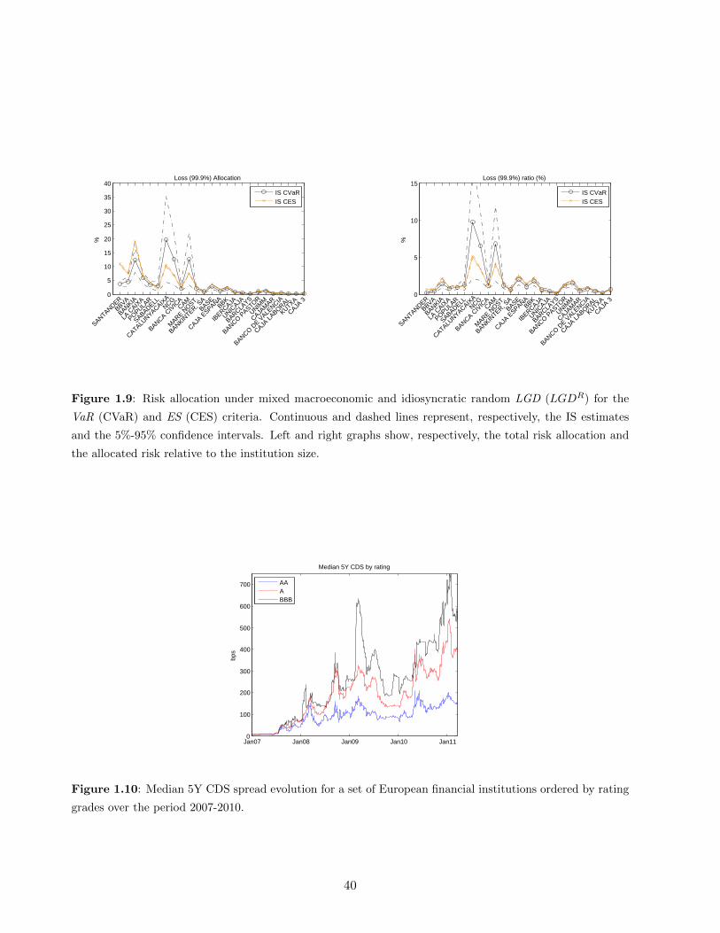
0
5
10
15
20
25
30
35
40
%
Loss (99.9%) Allocation
SANTANDER
BBVA
BANKIA
LA C
AIXA
POPULAR
SABADELL
CATALUNYACAIX
ANCG
BANCA CIV
ICACAM
MARE N
OST.
BANKINTER, S
ABASE
CAJA E
SPAÑABBK
IBERCAJA
UNICAJA
BARCLAYS
BANCO PASTOR
UNIMM
CAJAM
AR
BANCO DE V
ALENCIA
CAJA L
ABORAL
KUTXA
CAJA 3
IS CVaRIS CES
0
5
10
15
%
Loss (99.9%) ratio (%)
SANTANDER
BBVA
BANKIA
LA C
AIXA
POPULAR
SABADELL
CATALUNYACAIX
ANCG
BANCA CIV
ICACAM
MARE N
OST.
BANKINTER, S
ABASE
CAJA E
SPAÑABBK
IBERCAJA
UNICAJA
BARCLAYS
BANCO PASTOR
UNIMM
CAJAM
AR
BANCO DE V
ALENCIA
CAJA L
ABORAL
KUTXA
CAJA 3
IS CVaRIS CES
Figure 1.9: Risk allocation under mixed macroeconomic and idiosyncratic random LGD (LGDR) for the
VaR (CVaR) and ES (CES) criteria. Continuous and dashed lines represent, respectively, the IS estimates
and the 5%-95% confidence intervals. Left and right graphs show, respectively, the total risk allocation and
the allocated risk relative to the institution size.
Jan07 Jan08 Jan09 Jan10 Jan110
100
200
300
400
500
600
700
bps
Median 5Y CDS by rating
AAABBB
Figure 1.10: Median 5Y CDS spread evolution for a set of European financial institutions ordered by rating
grades over the period 2007-2010.
40

0 1 2 3 4 5 6 7 8 9 10
x 104
10−6
10−5
10−4
10−3
10−2
10−1
100
Loss Distribution
IS 10,000 x 100MC 1,000,000
6 6.5 7 7.5 8
x 104
10−3
Loss Distribution
IS 10,000 x 100MC 1,000,000
Figure 1.11: Loss distribution under the market mode. The black line shows the results of the Monte Carlo
(MC) method using 1,000,000 simulations. The red and blue lines show, respectively, the importance sampling
(IS) estimates and their 5%-95% confidence intervals using 10,000 macroeconomic scenarios and 100 default
simulations on each macroeconomic scenario.
0
10
20
30
40
50
%
Loss (99.9%) Allocation
SANTANDER
BBVA
BANKIA
LA C
AIXA
POPULAR
SABADELL
CATALUNYACAIX
ANCG
BANCA CIV
ICACAM
MARE N
OST.
BANKINTER, S
ABASE
CAJA E
SPAÑABBK
IBERCAJA
UNICAJA
BARCLAYS
BANCO PASTOR
UNIMM
CAJAM
AR
BANCO DE V
ALENCIA
CAJA L
ABORAL
KUTXA
CAJA 3
CVaRCES
0
1
2
3
4
5
%
Loss (99.9%) ratio (%)
SANTANDER
BBVA
BANKIA
LA C
AIXA
POPULAR
SABADELL
CATALUNYACAIX
ANCG
BANCA CIV
ICACAM
MARE N
OST.
BANKINTER, S
ABASE
CAJA E
SPAÑABBK
IBERCAJA
UNICAJA
BARCLAYS
BANCO PASTOR
UNIMM
CAJAM
AR
BANCO DE V
ALENCIA
CAJA L
ABORAL
KUTXA
CAJA 3
IS CVaRIS CES
Figure 1.12: Risk allocation under market valuation for the VaR (CVaR) and ES (CES) criteria. Continuous
and dashed lines represent, respectively, the IS estimates and the 5%-95% confidence intervals. Left and right
graphs show, respectively, the total risk allocation and the allocated risk relative to the institution size.
41

0 1 2 3 4 5 6 7 8
x 104
10−6
10−5
10−4
10−3
10−2
10−1
100
Loss Distribution
IS 10,000 x 100MC 1,000,000
1 1.1 1.2 1.3 1.4 1.5 1.6 1.7 1.8 1.9
x 104
10−3
Loss Distribution
IS 10,000 x 100MC 1,000,000
Figure 1.13: Loss distribution of the portfolio at December 2007 using 10,000 x 100 importance sampling
(IS) and 1,000,000 Monte Carlo (MC) simulations. The black and red lines show, respectively, the Monte
Carlo and IS results while the blue lines indicate the 5%-95% confidence interval of the IS estimates. Left
and right graphs show, respectively, the tail distribution and its detail in the neighborhood of the 99.9%
probability loss level.
0 1 2 3 4 5 6 7 8
x 104
10−6
10−5
10−4
10−3
10−2
10−1
100
Loss Distribution
M1, 0.5
M1, 0.75
M1, 0.9
M2
C1
C2
C3
Lo
2.8 3 3.2 3.4 3.6 3.8 4 4.2 4.4 4.6
x 104
10−3
10−2
Loss Distribution
M1, 0.5
M1, 0.75
M1, 0.9
M2
C1
C2
C3
Lo
Figure 1.14: Loss distribution of the portfolio at December 2010 under the different macroeconomic sensi-
tivity parameter estimates and using 10,000 x 100 importance sampling (IS) and 1,000,000 Monte Carlo (MC)
simulations. Left and right graphs show, respectively, the tail distribution and its detail in the neighborhood
of the 99.9% probability loss level.
42

0 1 2 3 4 5 6 7 8
x 104
10−6
10−5
10−4
10−3
10−2
10−1
100
Loss Distribution
IS 10,000 x 100MC 1,000,000
2.6 2.8 3 3.2 3.4 3.6 3.8 4 4.2 4.4
x 104
10−3
Loss Distribution
IS 10,000 x 100MC 1,000,000
Figure 1.15: Loss distribution of the portfolio at December 2010 under PD uncertainty and using 10,000 x
100 importance sampling (IS) and 1,000,000 Monte Carlo (MC) simulations. The black and red lines show,
respectively, the Monte Carlo and IS results while the blue lines indicate the 5%-95% confidence interval of the
IS estimates. Left and right graphs show, respectively, the tail distribution and its detail in the neighborhood
of the 99.9% probability loss level.
0 1 2 3 4 5 6 7 8
x 104
10−6
10−5
10−4
10−3
10−2
10−1
100
Loss Distribution
IS 10,000 x 100MC 1,000,000
4.2 4.4 4.6 4.8 5 5.2 5.4 5.6 5.8 6
x 104
10−3
Loss Distribution
IS 10,000 x 100MC 1,000,000
Figure 1.16: Loss distribution of the portfolio at December 2010 under LGD uncertainty and using 10,000
x 100 importance sampling (IS) and 1,000,000 Monte Carlo (MC) simulations. The black and red lines show,
respectively, the Monte Carlo and IS results while the blue lines indicate the 5%-95% confidence interval of the
IS estimates. Left and right graphs show, respectively, the tail distribution and its detail in the neighborhood
of the 99.9% probability loss level.
43
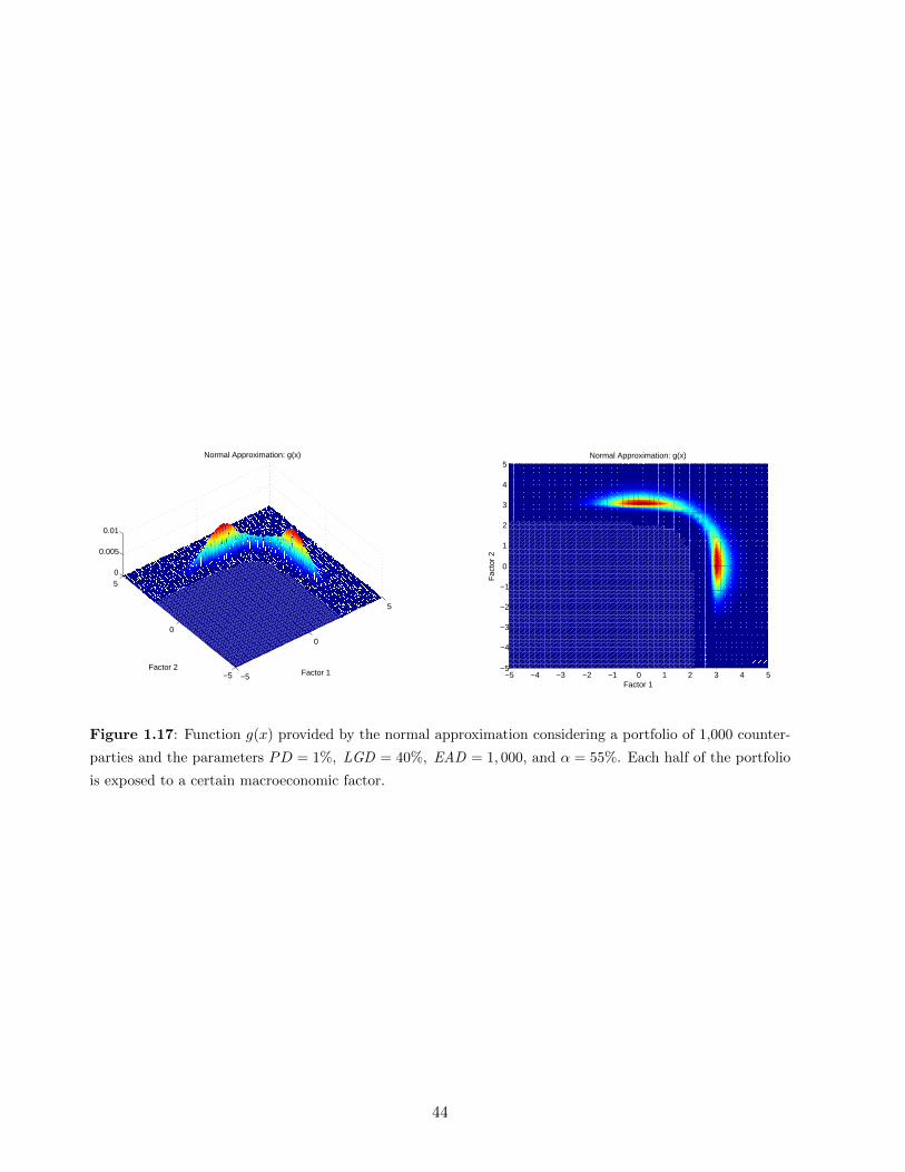
−5
0
5
−5
0
50
0.005
0.01
Factor 1
Normal Approximation: g(x)
Factor 2−5 −4 −3 −2 −1 0 1 2 3 4 5
−5
−4
−3
−2
−1
0
1
2
3
4
5
Factor 1
Normal Approximation: g(x)
Fac
tor
2
Figure 1.17: Function g(x) provided by the normal approximation considering a portfolio of 1,000 counter-
parties and the parameters PD = 1%, LGD = 40%, EAD = 1, 000, and α = 55%. Each half of the portfolio
is exposed to a certain macroeconomic factor.
44

Chapter 2
Extended saddlepoint methods for credit risk measurement
2.1 Introduction
This paper reviews and extends the saddlepoint methods currently available to measure credit risk.
We propose an approximate saddlepoint based method to allocate credit risk that, according to
our results, performs very well and even better than other alternatives currently available as, for
instance, Martin and Thompson (2001). We do also modify the default mode valuation saddlepoint
method to deal with random recoveries and market valuation. All these modifications are tested for
a portfolio including the Spanish financial institutions and compared with the results of a Monte
Carlo importance sampling method (IS) as a benchmark.
The credit risk loss distribution of a portfolio can be obtained in many ways being the Monte
Carlo simulation the simplest one, although it can be quite time consuming. As a consequence,
methods such as the importance sampling introduced in Glasserman and Li (2005) to speed up
the calculations have arisen. Other authors have developed approximate methods to estimate the
loss distribution of a portfolio, see Pykhtin (2004) or Voropaev (2011). The saddlepoint approach
is among these approximate alternatives. In more detail, this approach aims to approximate the
inverse Laplace transform of a certain function and, then, can be applied in many fields as statistics
and finance. In statistics it has been mainly used to approximate the distribution of the sum of
independent random variables, see Daniels (1954, 1980, 1987) or Reid (1988). More recently, the
saddlepoint method has been used to estimate the loss distribution of a loan portfolio, see Martin
and Thompson (2001) and Huang et al. (2007), among others.
Pure or importance sampling based Monte Carlo methods rely on simulations to estimate the loss
distribution and, hence, are exposed to sampling noise. In some cases, such as random idiosyncratic
recoveries, the confidence intervals of the Monte Carlo estimates get reduced very slowly as the
number of simulations increases (see Garcıa-Cespedes and Moreno (2014)). The saddlepoint method
proposed in Huang et al. (2007) is a semi-analytic technique that can be a reasonable candidate to
45

generate more stable estimates than a pure simulation one.
We show that the classic saddlepoint methods can be modified in a very intuitive way to deal with
pure macroeconomic random recoveries and market valuation. However in the case of idiosyncratic
random recoveries the saddlepoint methods can not be extended in a simple way and other methods
to obtain the inverse Laplace transform are required, see Abate and Whitt (1995).
This paper provides two major computational contributions to the literature. First, we propose
a risk allocation method based on the saddlepoint approach that, according to our results, is faster
and more accurate than other approaches previously analyzed in the literature. Second, we extend
the classic default mode saddlepoint model to deal with more realistic assumptions such as random
recoveries and market valuation.
Finally, for illustrative purposes, we consider the portfolio of the Spanish financial institutions
to test the accuracy of our extensions. In this way we quantify the risk of this financial system as a
whole and allocate it over the different financial entities. According to our results, our risk allocation
approximate method is more accurate than other alternatives such as that in Martin and Thompson
(2001) and requires a similar computational time. Compared with an exact risk allocation method,
we generate similar results but at a time cost that is independent on the number of counterparties
in the portfolio. The results for the random recoveries and the market valuation extensions are also
very close to those obtained with the Monte Carlo benchmark. However in this last case the number
of calculations increases considerably and the IS method can be more appropriate.
This paper is organized as follows. Section 2 introduces the first ideas of density and cumulative
distribution approximations using saddlepoint methods. Section 3 describes how to use saddlepoint
methods to measure credit risk and presents the new method to allocate risk based on the Hermite
polynomials and the random loss given default and market valuation extensions. Section 4 applies
the saddlepoint methods and our extensions to the portfolio of the Spanish financial institutions.
This Section shows how to calibrate the model parameters and how to obtain the portfolio loss
distributions and risk allocations. Finally, Section 5 summarizes our main results and concludes.
2.2 Saddlepoint methods
2.2.1 Density approximations
Let us define the moment and cumulant generating functions of a random variable x as Mx(t) =
E(ext) and Kx(t) = ln (Mx(t)), respectively. According to this, the moment generating function of
the sum of random variables L =∑M
j=1 xj is ML(t) = E(eLt). For independent random variables we
have that ML(t) =∏Mj=1Mxj (t) and KL(t) =
∑Mj=1Kxj (t).
Replicating the steps in Daniels (1987) let us define x = 1n
∑nj=1 xj . Using the cumulant gener-
46

ating function of x, Kx(t), we get the density function as the inverse Laplace transform
fx(x) =n
2πi
∫ c+i∞
c−i∞enKx(t)−ntxdt
Expanding the exponent in the integrand around a point t such that K ′x(t) = x, we have that
fx(x) =nen(Kx(t)−tx)
2πi
∫ c+i∞
c−i∞e∑∞q=2
nq!Kqx(t)(t−t)q
dt
where Kqx(t) = dqKx(t)dtq . Defining V =
√nK2x(t)(t− t), some computations lead to
fx(x) =nen(Kx(t)−tx)
2πi
∫ +i∞
−i∞eV 2
2A1√nK2x(t)
dV
where
A1 =∞∑i=0
1
i!
∞∑j=3
1
nj/2−1j!λjV
j
i
with λj = Kjx(t)(K2x(t))−j/2. Using that∫ +∞−∞ ikV ke−
V 2
2 dV = 0 for k odd and applying some
algebra, we get
fx(x) =nen(Kx(t)−tx)
2π
∫ +∞
−∞e−
V 2
2
(1 +
B1
n+C1
n2+ · · ·
)1√
nK2x(t)dV
where
B1 =1
24
(λ4V
4 − λ23V
6
3
)C1 =
1
144
(−λ6V
6
5+λ2
4V8
8− λ2
3λ4V10
12
)Previous integrals can be obtained using the statistical moments of a standard normal variable.
Then, considering the terms up to n−2, we get1
fx(x) ≈√nen(Kx(t)−tx)√
2πK2x(t)
[1 +
1
8n
(λ4 −
5λ23
3
)+
5
48n2
(−λ6
5+
7λ24
8− 21λ2
3λ4
4
)](2.1)
2.2.2 Cumulative distribution approximations
One way to obtain the cumulative probability distribution Fx(x) is to integrate the saddlepoint
approximation of fx(x) in (2.1). However this is not optimum because the density function fx(x)
1Daniels (1987) only shows the approximation up to terms in n−1.
47

must be integrated over a region but the approximation (2.1) is accurate just around a given point
x. The cumulative probability function can be obtained as
1− Fx(x) =1
2πi
∫ c+i∞
c−i∞
eKx(t)−tx
tdt, c > 0 (2.2)
In a similar way to the previous Subsection, Daniels (1987) applies a Taylor expansion to expres-
sion (2.2) and approximates the cumulative distribution by
P (X > x) =en(Kx(t)−tx)
2πi
∫ c+i∞
c−i∞en2K2x(t)(t−t)2A2
tdt
with
A2 =∞∑i=0
ni
i!
∞∑j=3
1
j!Kjx(t)(t− t)j
i
Defining z = t√nK2x(t) and z = t
√nK2x(t) provides
P (X > x) =en(Kx(t)−tx)+ z2
2
2πi
∫ c+i∞
c−i∞e
12z2−zzA3
zdz
with
A3 =∞∑i=0
1
i!
∞∑j=3
1
nj/2−1j!λj(z − z)j
i
Reordering we have
P (X > x) ≈ en(Kx(t)−tx)+ z2
2
[I0 +
λ3I3
6n0.5+
1
n
(λ4I4
24+λ2
3I6
72
)+
1
n1.5
(λ5I5
5!+λ3
3I9
3!4
)+
1
n2
(λ6I6
6!+λ2
4I8
2!4!2+ 3
λ4λ23I10
4!3!3
)]where
Ir =1
2πi
∫ c+i∞
c−i∞
(z − z)r
ze
12z2−zzdz, r = 0, 1, 2, · · ·
We have that I0 = P (z > z) = 1 − Φ(z) where Φ(·) indicates the distribution function of a
standard normal variable.2 Integration by parts provides the recursive relation Ir = ir−1φ(z)Mr−1−zIr−1 where φ(·) and Mi denote, respectively, the density function and the i-th moment of a standard
normal variable. Using this relation we have the next approximation for the cumulative probability
2The cumulant generating function of a normal random variable x ∼ N(µ, σ) is Kx(t) = µt+ 12σ2t2.
48

distribution up to the term n−1:
P (X > x) ≈ en(Kx(t)−tx)+ z2
2
[I0 +
λ3I3
6√n
+1
n
(λ4I4
24+λ2
3I6
72
)]= en(Kx(t)−tx)+ z2
2
[(1− Φ(z))
(1− λ3z
3
6√n
+1
n
(λ4z
4
24+λ2
3z6
72
))+φ(z)
(λ3(z2 − 1)
6√n
− 1
n
(λ4(z3 − z)
24+λ2
3(z5 − z3 + 3z)
72
))]Due to some technicalities the final saddlepoint approximation is
P (X > x) ≈
eKx(t)−tx+ z2
2 [(1− Φ(z))B2 + φ(z)C2] X > E(x)12 X = E(x)
1− eKx(t)−tx+ z2
2 [(1− Φ(z))B2 + φ(z)C2] X < E(x)
(2.3)
with
B2 = 1− λ3z3
6+λ4z
4
24+λ2
3z6
72
C2 =λ3(z2 − 1)
6− λ4(z3 − z)
24− λ2
3(z5 − z3 + 3z)
72
2.3 Credit risk and saddlepoint approximation
2.3.1 Saddlepoint method for credit risk
According to the Vasicek (1987) model the default behavior of the client j is driven by a set of
random macroeconomic factors Z = z1, z2, · · · , zk and an idiosyncratic random term εj . This
idiosyncratic term is a client specific random variable. The factors ziki=1 and εj are independent
and distributed as standard normal random variables. Given this specification, the default of this
client is modeled through the asset value variable Vj , defined as
Vj =
k∑f=1
αf,jzf + εj
√√√√1−k∑
f=1
α2f,j
where the terms αf,j capture the macroeconomic sensitivity of the asset value. Then, the client j
defaults if Vj falls below a threshold level k. By construction Vj ∼ N(0, 1) and k equates Φ−1(PDj,C),
where PDj,C denotes the historical average default probability of the client j.
The total loss of a portfolio including M contracts or clients is given as L =∑M
j=1 xj , where xj
is the individual loss of the client or contract j. According to this the portfolio loss can be expressed
using the exposure at default (EADj) and the loss given default (LGDj) parameters of each client
as
L =
M∑j=1
xj =
M∑j=1
EADjLGDj1(Vj ≤ Φ−1(PDj,C))
49

In the case of default mode models with constant LGD, the cumulants of the loss distribution
conditional to a macroeconomic scenario can be obtained in a very simple way. Conditional to
a given macroeconomic scenario, the defaults are independent and the cumulants of the sum of
independent random variables are given by the sum of the cumulants of each random variable. Then,
assuming that the portfolio is made up of M clients with default probability PDj(Z) conditional to
the scenario Z, the cumulant generating function of the loss distribution L =∑M
j=1 xj is given by
Kx(t) =∑M
j=1 kx(j, t) with kx(j, t) = ln(1 − PDj(Z) + PDj(Z)etwj ) where wj = EADj × LGDj .
The derivatives of Kx(t) can be easily computed up to any order by applying a recursive relation.3
Based on these cumulants, an approximation for P(∑M
j=1 xj > l∣∣∣ Z) can be obtained for dif-
ferent values of Z and then empirically estimate E(P(∑M
j=1 xj > l∣∣∣ Z)). Under the usual credit
risk framework, the scenarios Z are distributed as N(0,Σ) and can be simulated using Monte Carlo
techniques.
For heavily concentrated portfolios the usual saddlepoint approximation is not accurate and a
modification is required. This modification is called adaptative saddlepoint approximation and was
proposed in Huang et al. (2007). Consider a portfolio where the firms A and B are the two biggest
counterparties in terms of the final loss given default (EAD × LGD). Let xA and xB be the LGDs
(in currency units) of these firms and consider l ∈ (xB, xA). Then, P (L > x|Z) can be obtained as
P
M∑j=1
xj ≥ l
∣∣∣∣∣∣Z = 1− P
M∑j=1
xj < l
∣∣∣∣∣∣Z
= 1− (1− PDA(Z))P
M∑j 6=A
xj < l
∣∣∣∣∣∣Z
= 1− (1− PDA(Z))
1− P
M∑j 6=A
xj ≥ l
∣∣∣∣∣∣Z
= 1− (1− PDA(Z))(1− Sad(LA, l, Z)) (2.4)
where LA represents the loss of the portfolio excluding the client A and Sad(LA, l, Z) stands for
the saddlepoint approximation of the cumulative probability of LA for a loss level l and conditional
to a macroeconomic scenario Z. If the loss level is just below xB, expression (2.4) becomes
P
M∑j=1
xj ≥ l
∣∣∣∣∣∣Z = 1− (1− PDA(Z))(1− PDB(Z))(1− Sad(LA,B, l, Z))
In a similar way, the density distribution can be written as fL(l|Z) = (1− PDA)Sadf (LA, l, Z).
3Details are available upon request. It can be observed that the first derivative is equivalent to the exponential
twist of the conditional default probabilities proposed in the IS framework by Glasserman and Li (2005).
50

2.3.2 Risk contributions
The two most extended ways to allocate the risk of a portfolio among its different counterparties are
the Value-at-Risk (VaR) contribution (CVaR) and the expected shortfall (ES) contribution (CES).
Both measures indicate, respectively, the contribution of a client to a given percentile and to a given
conditional moment of the loss distribution. The main reason for considering a moment rather than
a percentile is that, under the usual Monte Carlo framework, the stability of the CES is much higher
than that of the CVaR.
According to the CVaR criterion, the risk contribution of the client j is
CV aRj = E
xj∣∣∣∣∣∣M∑j=1
xj = V aR
=E(xj1(
∑Mj=1 xj = V aR))
f(∑M
j=1 xj = V aR)
= wjE(f(Dj = 1, L = V aR|Z))
E(f(L = V aR|Z))
= wjE(f(Lj = V aR− wj |Z)PDj(Z))
E(f(L = V aR|Z))(2.5)
where Lj =∑M
k 6=j xk is the loss of the total portfolio excluding the client j.
For the ES contribution, a similar formula can be derived
CESj = wjE(P (Lj > V aR− wj |Z)PDj(Z))
E(P (Lj > V aR|Z))(2.6)
Then if we want to use saddlepoint methods we need to approximate f(Lj = V aR− wj |Z) and
P (Lj > V aR − wj |Z) for each client j. This requires to estimate a different saddlepoint for each
client and macroeconomic scenario, a very time demanding procedure.
To obtain the CV aR of each client, an alternative way that avoids this client by client estimation
is proposed in Martin and Thompson (2001) who suggested a formula that depends on the derivatives
of the cumulant generating function of the whole portfolio and that, after some algebra, becomes
CV aRj ≈E
(f(L = V aR|Z)wj
PDj(Z)ewj t
1−PDj(Z)+PDj(Z)ewj t
)E(f(L = V aR|Z))
However, some papers as Huang et al. (2007) have suggested that this approximate formula may
be not accurate enough. Then, we have decided to take a different approach. From now on, we
consider that the saddlepoint of the whole portfolio loss L in the point l = V aR conditional to a
given macroeconomic scenario, tZ , should be close to tj,Z , the saddlepoint of the portfolio once the
client j is removed in the point l = V aR− wj .4
4This is a reasonable assumption if the portfolio is not very concentrated.
51

As a result we try to approximate the density and distribution functions of Lj around l =
V aR − wj using the value tZ rather than tj,Z . Of course, as tZ is not the real saddlepoint of the
portfolio loss Lj in l = V aR− wj , some adjustments will be required in formulas (2.1) and (2.3).
Tsao (1995) provided the detailed steps to obtain the adjustments to extend expression (2.1)
and approximate f(Lj = V aR − wj |Z) around a general point tZ . Using a Taylor expansion of the
exponent in the integral, we know that
fx(x) =1
2πi
∫ c+i∞
c−i∞eKx(t)−txdt
=eKx(tZ)−tZx
2π
∫ ∞−∞
e(K′x(tZ)−x)it+1/2K2x(tZ)(it)2+1/6K3x(tZ)(it)3+···dt
=eKx(tZ)−tZx
2π
∫ ∞−∞
e−K2x(tZ )
2(t−ci)2− (K′x(tZ )−x)2
2K2x(tZ )+1/6K3x(tZ)(it)3+···
dt
=eKx(tZ)−tZx−
(K′x(tZ )−x)2
2K2x(tZ )
2π
∫ ∞−∞
e−K2x(tZ )
2(t−ci)2+1/6K3x(tZ)(it)3+···dt
where c = K′x(tZ)−xK2x(tZ) . Defining V =
√K2x(tZ)(t − ci), expanding the exponential function, and
working with the imaginary terms provides
fx(x) =eKx(tZ)−tZx−
(K′x(tZ )−x)2
2K2x(tZ )√2πK2x(tZ)
∫ ∞−ic√K2x(tZ)
−∞−ic√K′′x (tZ)
φ(V )
×
1 +
∞∑j=3
λjx(tZ)
j!(iV − c
√K2x(tZ))j +
1
2
∞∑j=3
λjx(tZ)
j!(iV − c
√K2x(tZ))j
2
+ · · ·
dV
As the integrand is an analytic function, the integration limits can be changed to ±∞. Moreover,
we have ∫ ∞−∞
φ(V )(iV − x)kdV = (−1)kHk(x)
where Hk(x) is the k-th order Hermite polynomial.5
Finally we have
fx(x) =eKx(tZ)−tZx−
(K′x(tZ )−x)2
2K2x(tZ )√2πK2x(tZ)
[1− λ3x(tZ)
6H3
(K ′(tZ)− x√K ′′(tZ)
)
+λ4x(tZ)
24H4
(K ′(tZ)− x√K ′′(tZ)
)+λ3x(tZ)2
72H6
(K ′(tZ)− x√K ′′(tZ)
)+ · · ·
](2.7)
5See Abramowitz and Stegun (1964) for details.
52
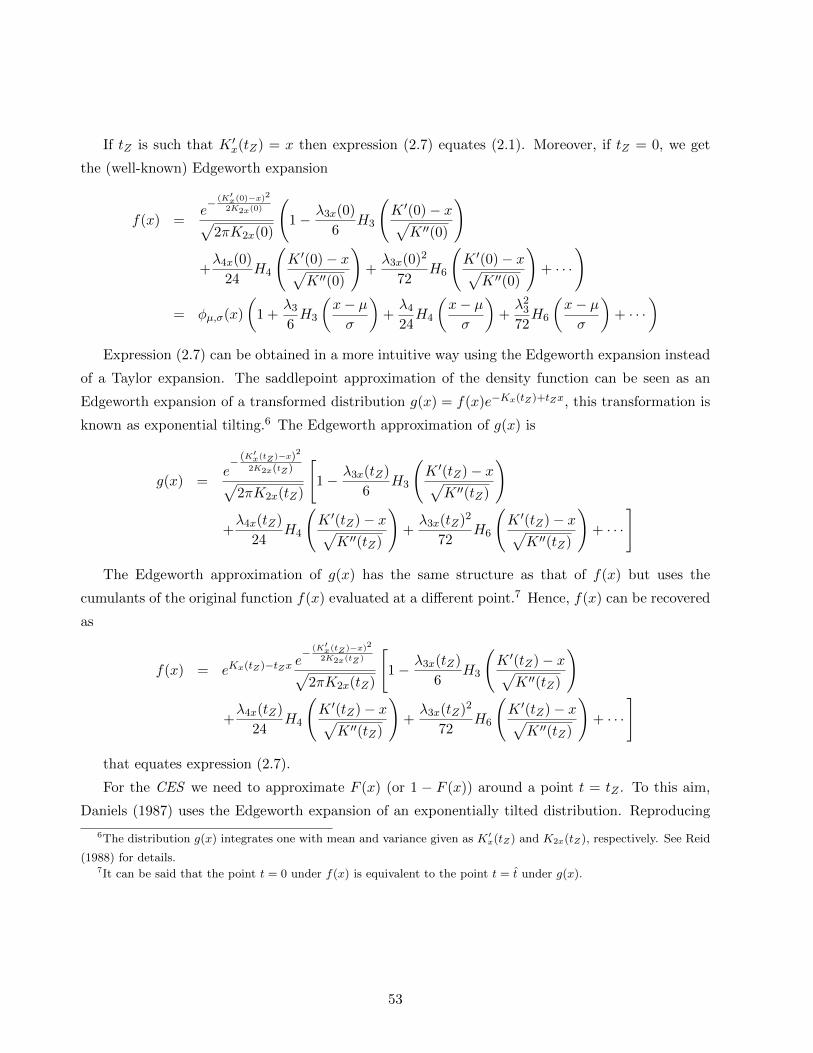
If tZ is such that K ′x(tZ) = x then expression (2.7) equates (2.1). Moreover, if tZ = 0, we get
the (well-known) Edgeworth expansion
f(x) =e− (K′x(0)−x)2
2K2x(0)√2πK2x(0)
(1− λ3x(0)
6H3
(K ′(0)− x√K ′′(0)
)
+λ4x(0)
24H4
(K ′(0)− x√K ′′(0)
)+λ3x(0)2
72H6
(K ′(0)− x√K ′′(0)
)+ · · ·
)
= φµ,σ(x)
(1 +
λ3
6H3
(x− µσ
)+λ4
24H4
(x− µσ
)+λ2
3
72H6
(x− µσ
)+ · · ·
)Expression (2.7) can be obtained in a more intuitive way using the Edgeworth expansion instead
of a Taylor expansion. The saddlepoint approximation of the density function can be seen as an
Edgeworth expansion of a transformed distribution g(x) = f(x)e−Kx(tZ)+tZx, this transformation is
known as exponential tilting.6 The Edgeworth approximation of g(x) is
g(x) =e− (K′x(tZ )−x)2
2K2x(tZ)√2πK2x(tZ)
[1− λ3x(tZ)
6H3
(K ′(tZ)− x√K ′′(tZ)
)
+λ4x(tZ)
24H4
(K ′(tZ)− x√K ′′(tZ)
)+λ3x(tZ)2
72H6
(K ′(tZ)− x√K ′′(tZ)
)+ · · ·
]
The Edgeworth approximation of g(x) has the same structure as that of f(x) but uses the
cumulants of the original function f(x) evaluated at a different point.7 Hence, f(x) can be recovered
as
f(x) = eKx(tZ)−tZx e− (K′x(tZ )−x)2
2K2x(tZ )√2πK2x(tZ)
[1− λ3x(tZ)
6H3
(K ′(tZ)− x√K ′′(tZ)
)
+λ4x(tZ)
24H4
(K ′(tZ)− x√K ′′(tZ)
)+λ3x(tZ)2
72H6
(K ′(tZ)− x√K ′′(tZ)
)+ · · ·
]
that equates expression (2.7).
For the CES we need to approximate F (x) (or 1 − F (x)) around a point t = tZ . To this aim,
Daniels (1987) uses the Edgeworth expansion of an exponentially tilted distribution. Reproducing
6The distribution g(x) integrates one with mean and variance given as K′x(tZ) and K2x(tZ), respectively. See Reid
(1988) for details.7It can be said that the point t = 0 under f(x) is equivalent to the point t = t under g(x).
53

his steps we have that
1− F (x) =
∫ ∞x
f(y)dy
= eK(tZ)−tZx∫ +∞
xe−tZ(y−x)f(y)etZy−K(tZ)dy
= eK(tZ)−tZx∫ +∞
x
e−tZ(y−x)√K ′′(tZ)
φ
(K ′(tZ)− y√K ′′(tZ)
)[1− λ3x(tZ)
6H3
(K ′(tZ)− y√K ′′(tZ)
)
+λ4x(tZ)
24H4
(K ′(tZ)− y√K ′′(tZ)
)+λ3x(tZ)2
72H6
(K ′(tZ)− y√K ′′(tZ)
)+ · · ·
]dy
= eK(tZ)−tZx∫ v
−∞e−tZ(K′(tZ)−x−V
√K′′(tZ))φ(V )
×[1− λ3x(tZ)
6H3(V ) +
λ4x(tZ)
24H4(V ) +
λ3x(tZ)2
72H6(V ) + · · ·
]dV
= eK(tZ)−tZK′(tZ)
∫ v
−∞etZ(V
√K′′(tZ))φ(V )
×[1− λ3x(tZ)
6H3(V ) +
λ4x(tZ)
24H4(V ) +
λ3x(tZ)2
72H6(V ) + · · ·
]dV
= eK(tZ)−tZK′(tZ)+t2ZK
′′(tZ )
2
×[I0(v)− λ3x(tZ)
6I3(v) +
λ4x(tZ)
24I4(v) +
λ3x(tZ)2
72I6(v) + · · ·
](2.8)
with
v =K ′(tZ)− x√K ′′(tZ)
Ii(v) =
∫ v
−∞e−
t2ZK′′(tZ )
2+tZV
√K′′(tZ)φ(V )Hi(V )dV =
∫ v
−∞φ(V − a)Hi(V )dV
where a = tZ√K ′′(tZ). As in the previous Section we have that I0(v) = Φ(v − a) and integrating
Ii by parts leads to the recursive relation Ii(v) = −φ(v − a)Hi−1(v) + aIi−1(v) that can be very
easily implemented in a computer.
Truncating equation (2.8) at I3(v) and using a point tZ such that K ′(tZ) = x’ provides the
saddlepoint approximation in expression (2.3)
1− F (x) ≈ e(K(tZ)−tK′(tZ))+t2ZK
′′(tZ )
2
[(1− Φ(a))
(1− a3λ3x(tZ)
6
)+ φ(a)
(a2 − 1)λ3x(tZ)
6
]As before, if tZ = 0, then a = 0, I0(v) = Φ(v), and Ii(v) = −φ(v)Hi−1(v). Then, we get the
Edgeworth expansion
1− F (x) = Φ(v)− φ(v)
(−λ3
6H2(v) +
λ4
24H3(v) +
λ23
72H5(v) + · · ·
)54

The approximations in (2.7) and (2.8) are named Hermite polynomials based saddlepoint approx-
imations (Sad-Her). Using these formulas the estimation of the risk contributions requires much less
time as, for each macroeconomic scenario, we do not need to estimate a saddlepoint for each client
and we can use a unique value tZ . Later, the empirical Section will show that these formulas pro-
vide a much better accuracy than the Martin’s approximation and with similar results to the exact
method.
2.3.3 Random LGD models
The loss given default (LGD) is usually considered to be constant although it can be a random
variable. The two simplest ways to model LGD as a random variable are, respectively, constant
or random LGD conditional to a given macroeconomic scenario, Z. We discuss now these two
alternatives.
1. In the first case (LGDC), the saddlepoint approximation method does not need any modifica-
tion and, for each macroeconomic scenario, we have to use LGDi(Z) instead of LGDi. This
way to introduce the random LGD behavior implies no restriction on the functional form of the
LGD that can be used. Table 2.1 includes several possible pure macroeconomic LGD models
(LGDC |z), where z represents a set of macroeconomic factors driving the recoveries behavior.
A usual assumption is that these factors follow a standard normal distribution.
[INSERT TABLE 2.1 AROUND HERE]
Calibrating these pure macroeconomic LGD models is not complex, assuming a single macroe-
conomic LGD factor zLGD with a standard normal distribution we can obtain expressions for
the unconditional mean and variance that depend only on the parameters a and b in Table
2.1.8 Then using a time series of average LGDs (LGDt1 , LGDt2 , · · · , LGDty) we can calibrate
the parameters that best fit these two moments.
After estimating the parameters a and b we can recover the time series of the LGD and default
driving macroeconomic factors, zLGD,t1 , zLGD,t2 , · · · , zLGD,ty and zPD,t1 , zPD,t2 , · · · , zPD,tyand, then, we can calibrate the correlation between both factors, ρzPD,zLGD .
2. In the case of the random conditional LGD (LGDR), the saddlepoint approximation requires
to consider the moment generating function of the random variable LGDi(Z) of each client in
8This can be done for all the distributions in Table 2.1 but for the logit and probit distributions. For these two
cases a Monte Carlo method was implemented to calibrate the parameters.
55

the portfolio (MLGDi|Z(EADit)). Now, the cumulants of the portfolio are
Kx(t) =M∑j=1
ln[1− PDj(Z) + PDj(Z)MLGDj |Z(EADjt)]
Then, not all the distributions are suitable to characterize the LGD behavior. The most
common continuous random variables with known moment generating function are the normal,
gamma, and beta distributions.9 Table 2.2 includes the different models that will be analyzed
in the empirical Section.
[INSERT TABLE 2.2 AROUND HERE]
Under random conditional recoveries the calibration of the LGD model parameters is much
more complex. For the gamma and beta distributions we sample numerically from these
distributions to obtain the parameters a, b, and c in Table 2.2 that provide the best fit
to the values E(LGDR
), V ar
(LGDR
), and E
(V ar
(LGDR|zLGD
))of the real recoveries
sample.10 As in the previous case, after estimating these parameters, we can recover a time
series of zLGD,t1 , zLGD,t2 , · · · , zLGD,ty and estimate ρzPD,zLGD , the correlation between the
macroeconomic default driving factor and the recoveries driving factor.
The extension of the adaptative saddlepoint approximation gets slightly more complex. Now,
for l ∈ (xB, xA), the probability P (L > l|Z) is given as
P
M∑j=1
xj ≥ l
∣∣∣∣∣∣ Z = 1−
∫ l
0fA(y|Z)P
M∑j 6=A
xj < l − y
∣∣∣∣∣∣ Z dy
where fA(y) stands for the loss distribution of a portfolio including just the counterparty A.
This integral can be obtained approximating the probability inside the integrand using the
saddlepoint method and applying numerical integration. However this method gets complex
and slow and we think that other methods to obtain the inverse Laplace transform can provide
better results. Reproducing the ideas in Abate and Whitt (1995) and Glasserman and Ruiz-
Mata (2006) we have
1− Fx(x) =1
2πi
∫ c+i∞
c−i∞
eKx(t)−tx
tdt =
2e−cx
π
∫ ∞0
Re
(eKx(c+ui)
c+ ui
)cos(ux)du
9See the Appendix for further details.10The calibration of the normal idiosyncratic LGD can be done without the Monte Carlo sampling process as its
conditional and unconditional moments are straightforward.
56

The numerical approximation for this integral provides
1− Fx(x) ≈ e−cx∆u
π
[Re
(eKx(c)
c
)+ 2
N∑k=1
Re
(eKx(c+ik∆u)
c+ ik∆u
)cos(xk∆u)
](2.9)
Later, the empirical Section will show that this method to obtain the inverse Laplace transform
is very accurate once the model parameters have been carefully chosen. However, the time
required to obtain the numerical integral is much higher than that of the saddlepoint methods.
In the case of the risk allocation under random conditional recoveries, the number of calcula-
tions needed to implement the VaR and ES based risk contribution formulas increases consid-
erably and the time advantage of the approximate methods completely disappears. Then, we
decide to stop here the methodological analysis of the saddlepoint and inverse Laplace trans-
form methods for the default mode models.The next Subsection will extend the saddlepoint
method to the case of market valuation.
2.3.4 Market mode models
Under a market valuation model the rating of a firm may change over time and these changes affect
the firm value and can generate losses. Then we need to compute Vi,h, the value of the client i under
any of the possible rating states h.
To build the state migration rule, let MPj,C,IR,FR denote the average (over the cycle) migration
probability from an initial rating IR to a final rating state FR for the client j. Then we can
compute AccumMPj,Z,IR,FR, the accumulated probabilities for all the possible final rating states
FR = AAA,AA+, · · · , CCC,D.11
For a given macroeconomic state z, we can calculate the point in time accumulated probability
of migration between ratings, AccumMPj,Z,IR,FR, as
AccumMPj,Z,IR,FR = Φ
Φ−1(AccumMPj,C,IR,FR)−∑k
f=1 αf,jzf√1−
∑kf=1 α
2f,j
From these conditional accumulated probabilities we can recover the non accumulated ones.
Under market valuation the cumulant generating function of the portfolio value function is given by
Kx(t) =
M∑j=1
ln
(s∑
h=1
MPj,Z,IR,hetVj,h
)(2.10)
We can work with the market mode value Vj,h or, inversely, xM,j,h, the losses of each client j at
each state h. As we did in the default mode, using the cumulant generating function (2.10) we can
11For example, AccumMPj,Z,IR,B− = MPj,Z,IR,B− +MPj,Z,IR,CCC +MPj,Z,IR,D.
57

approximate the loss distribution of the portfolio and the risk contributions. We need to extend the
adaptative saddlepoint approximation. Focusing on the losses of the portfolio, we get
P
M∑j=1
xM,j,h ≥ l
∣∣∣∣∣∣Z = 1− P (xM,j,h < l|Z)P
M∑j=1
xM,j,h < l
∣∣∣∣∣∣ xM,j,h < l, Z
(2.11)
As it can be seen, we have to condition on all the possible final states h where the losses of the
client j do not exceed l. Recall that, under the default mode, for each client there was only one final
state that could generate losses greater than l. Now, under the market valuation, there may exist
several states that generate these high losses. We must also note that the expression (2.11) is true
as long as losses are positive.12
Regarding the risk allocation, the VaR and ES contributions of the client j are given by
CV aRi = E
xM,j,h
∣∣∣∣∣∣M∑j=1
xM,j,h = V aR
=E (∑s
h=1 xM,j,hf(hj |z)f(LM,j = V aR− xM,j,h|z))E (f (LM = V aR|Z))
CESj =E (∑s
h=1 xM,j,hf (hj |z) f (LM,j > V aR− xM,j,h|z))E (P (LM > V aR|Z))
with LM =∑M
j=1 xM,j,h and LM,j =∑M
k 6=j xM,k,h.
Note that the expression of CVaR and CES under the market valuation are very similar to those
for the default mode but, in the numerator, we sum over all the possible final rating states and,
hence, we have to estimate a saddlepoint for each client, final rating, and macroeconomic scenario.
Therefore, the use of the Hermite polynomials based saddlepoint approximations becomes a very
interesting tool as we must estimate just one saddlepoint tZ for each macroeconomic scenario and
maintain it for all the different clients and final rating states.
2.4 Empirical analysis
This Section illustrates empirically the theoretical framework and the extensions that we have pro-
posed in previous Sections. In more detail, we consider a portfolio that includes the Spanish financial
institutions at December 2010 and obtain the loss distribution and the risk contribution of each en-
tity. We start introducing this portfolio and describing the data sources that we have employed to
obtain the main risk drivers of the portfolio. Later, we obtain the loss distribution and the risk
allocation of these institutions for the case of constant and random LGDs and for market valuation
losses. In all the cases, the results from a Monte Carlo importance sampling method are used as
benchmark. Finally, we do also test the Hermite polynomials based saddlepoint method that we
have proposed to allocate the risk.
12This is the case for losses on total notional or on best state valuation but not necessarily for losses on current state
valuation.
58
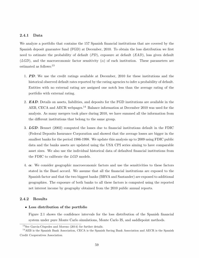
2.4.1 Data
We analyze a portfolio that contains the 157 Spanish financial institutions that are covered by the
Spanish deposit guarantee fund (FGD) at December, 2010. To obtain the loss distribution we first
need to estimate the probability of default (PD), exposure at default (EAD), loss given default
(LGD), and the macroeconomic factor sensitivity (α) of each institution. These parameters are
estimated as follows:13
1. PD : We use the credit ratings available at December, 2010 for these institutions and the
historical observed default rates reported by the rating agencies to infer a probability of default.
Entities with no external rating are assigned one notch less than the average rating of the
portfolio with external rating.
2. EAD : Details on assets, liabilities, and deposits for the FGD institutions are available in the
AEB, CECA and AECR webpages.14 Balance information at December 2010 was used for the
analysis. As many mergers took place during 2010, we have summed all the information from
the different institutions that belong to the same group.
3. LGD : Bennet (2002) computed the losses due to financial institutions default in the FDIC
(Federal Deposits Insurance Corporation and showed that the average losses are bigger in the
smallest banks for the period 1986-1998. We update this analysis up to 2009 using FDIC public
data and the banks assets are updated using the USA CPI series aiming to have comparable
asset sizes. We also use the individual historical data of defaulted financial institutions from
the FDIC to calibrate the LGD models.
4. α: We consider geographic macroeconomic factors and use the sensitivities to these factors
stated in the Basel accord. We assume that all the financial institutions are exposed to the
Spanish factor and that the two biggest banks (BBVA and Santander) are exposed to additional
geographies. The exposure of both banks to all these factors is computed using the reported
net interest income by geography obtained from the 2010 public annual reports.
2.4.2 Results
• Loss distribution of the portfolio
Figure 2.1 shows the confidence intervals for the loss distribution of the Spanish financial
system under pure Monte Carlo simulations, Monte Carlo IS, and saddlepoint methods.
13See Garcıa-Cespedes and Moreno (2014) for further details.14AEB is the Spanish Bank Association, CECA is the Spanish Saving Bank Association and AECR is the Spanish
Credit Cooperatives Association.
59

[INSERT FIGURE 2.1 AROUND HERE]
It can be seen that the accuracy of the saddlepoint approximation is quite bad for loss levels
below 53,146 MM e, a value that indicates the LGD of Santander, the biggest institution in
our sample. This result is expected as we are not using the adaptative saddlepoint approx-
imation. Figure 2.2 shows the loss distribution considering this modification and illustrates
that the accuracy of the saddlepoint approximation increases considerably. As in the previous
Figure, we provide the results from the saddlepoint approximation with 1,000 macroeconomic
scenarios15, a pure Monte Carlo method with 1,000,000 simulations, and a Monte Carlo IS
method with 1,000 x 100 simulations. The 99.9% probability loss level is 31,352 MMe, a value
that will be used in the next issues.
[INSERT FIGURE 2.2 AROUND HERE]
• Risk contribution of each financial institution
We test the accuracy of the Hermite polynomials based saddlepoint approximations (Sad-Her)
(see equations (2.7)-(2.8)) to estimate the risk contributions (see equations (2.5)-(2.6)) for
a loss level of 31,352 MMe. The results of these approximations are compared with those
obtained using a pure Monte Carlo method (MC), the Monte Carlo IS method (IS), the exact
saddlepoint approximation (Sad), and the method proposed in Martin and Thompson (2001)
(Sad-Mar). Figures 2.3 and 2.4 show the results for the VaR and ES risk allocation simulating,
respectively, 100 and 1,000 macroeconomic scenarios.
[INSERT FIGURES 2.3 AND 2.4 AROUND HERE]
Figure 2.3 shows that, for the VaR based risk allocation, all the methods except the Martin’s
one produce very similar risk allocations. This is the case even though the IS and the saddle-
point methods use a very small number of macroeconomic scenarios. It is worth to mention
that the risk allocated to BBVA and Santander is null. This is because their LGDs are higher
than 31,352 MMe and, then, they can not have defaulted conditional to scenarios that gener-
ate a total portfolio loss of 31,352 MMe. For the ES based risk allocation, the results for the
IS and the saddlepoint methods are very close to each other16 but very far from those of the
15The mean of the macroeconomic scenarios is changed and a weighting function is introduced according to the ideas
in Glasserman and Li (2005). However, the shift in the mean of the macroeconomic variables is done according to the
mean (and not to the mode) of the optimum distribution. See Garcıa-Cespedes and Moreno (2014) for further details.16Both methods share the same macroeconomic scenarios in the simulation process.
60
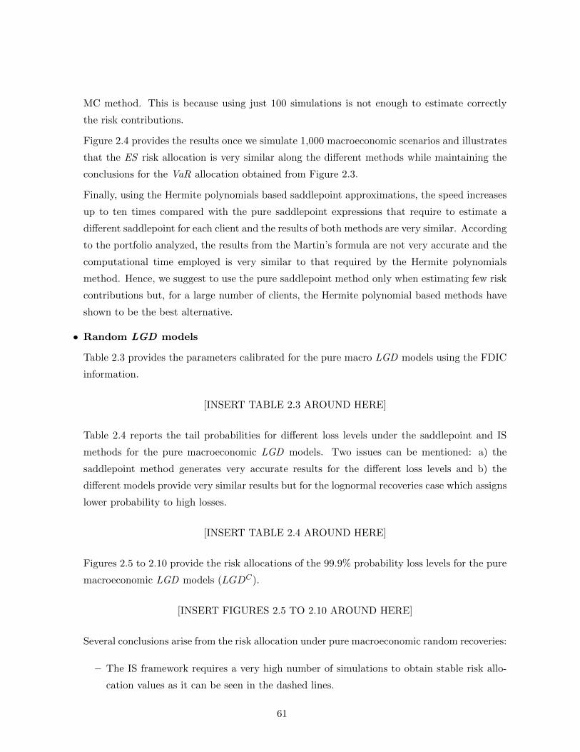
MC method. This is because using just 100 simulations is not enough to estimate correctly
the risk contributions.
Figure 2.4 provides the results once we simulate 1,000 macroeconomic scenarios and illustrates
that the ES risk allocation is very similar along the different methods while maintaining the
conclusions for the VaR allocation obtained from Figure 2.3.
Finally, using the Hermite polynomials based saddlepoint approximations, the speed increases
up to ten times compared with the pure saddlepoint expressions that require to estimate a
different saddlepoint for each client and the results of both methods are very similar. According
to the portfolio analyzed, the results from the Martin’s formula are not very accurate and the
computational time employed is very similar to that required by the Hermite polynomials
method. Hence, we suggest to use the pure saddlepoint method only when estimating few risk
contributions but, for a large number of clients, the Hermite polynomial based methods have
shown to be the best alternative.
• Random LGD models
Table 2.3 provides the parameters calibrated for the pure macro LGD models using the FDIC
information.
[INSERT TABLE 2.3 AROUND HERE]
Table 2.4 reports the tail probabilities for different loss levels under the saddlepoint and IS
methods for the pure macroeconomic LGD models. Two issues can be mentioned: a) the
saddlepoint method generates very accurate results for the different loss levels and b) the
different models provide very similar results but for the lognormal recoveries case which assigns
lower probability to high losses.
[INSERT TABLE 2.4 AROUND HERE]
Figures 2.5 to 2.10 provide the risk allocations of the 99.9% probability loss levels for the pure
macroeconomic LGD models (LGDC).
[INSERT FIGURES 2.5 TO 2.10 AROUND HERE]
Several conclusions arise from the risk allocation under pure macroeconomic random recoveries:
– The IS framework requires a very high number of simulations to obtain stable risk allo-
cation values as it can be seen in the dashed lines.
61

– The introduction of the random LGD increases the risk allocated to the two biggest
financial institutions.
– Even for a small number of simulations, the pure saddlepoint method generates very
accurate risk allocation results although it is very time consuming.
– Compared to the pure saddlepoint approach, the Hermite polynomials based saddlepoint
method generates very close results and is much faster.
Table 2.5 shows the parameters calibrated for the mixed macro and idiosyncratic LGD models
using the FDIC information.
[INSERT TABLE 2.5 AROUND HERE]
To get the loss distribution under idiosyncratic recoveries we use the method to obtain the
inverse Laplace transform described in Subsection 3.3. Following Abate and Whitt (1995), the
Euler summation method can be used to increase the convergence speed.17 We will use c = t
where K ′x(t) = x and ∆u = t10 aiming to guarantee that eKx(c+ik∆u) can be computed and
that the distance between Re(eKx(c+i(k−1)∆u)
c+i(k−1)∆u
)and Re
(eKx(c+ik∆u)
c+ik∆u
)is reasonably small.
To obtain the loss distribution we first define a vector Vl = (l1, l2, · · · , lN ) of loss levels whose
mean l is considered a representative loss value. Then, we obtain t(l, Z) for each macroeconomic
scenario and estimate 1 − Fx(Vl|Z) using t(l, Z) and equation (2.9). Finally we compute the
weighted average of the estimates of 1− Fx(Vl|Z) over all the simulated scenarios Z.
This method to estimate the loss distribution is faster than that in Abate and Whitt (1995) as,
now, the values c and ∆u do not depend on the loss level li. Hence, Re(eKx(c+2ik∆u)
a+2ik∆u
)remains
constant for every loss value in Vl and the number of calculations required to estimate the loss
distribution is reduced.
Table 2.6 provides the tail probabilities for different loss levels for the different mixed macroe-
conomic and idiosyncratic LGD models under saddlepoint and IS methods. It can be observed
that the Laplace inversion method generates very accurate results.
[INSERT TABLE 2.6 AROUND HERE]
Comparing Tables 2.4 and 2.6 we can see that the loss distributions under the mixed idiosyn-
cratic and macroeconomic LGD model are very close to those under the pure macro LGD
17This method approximates the sum of a series using the first Nd terms plus a weighted sum of Nl terms that uses
the first Nd terms.
62

model. Then, we can say that, at least for the portfolio under analysis, modeling the idiosyn-
cratic behavior of the recoveries is not important to measure the loss distribution.
Finally, using the inverse Laplace transform to recover the loss distribution requires much more
time than the saddlepoint method. This gets even worse for the beta LGD distribution as we
must evaluate numerically the moment generating function of the beta distribution.18 Com-
pared with a pure Monte Carlo or an IS method, the time required to solve the idiosyncratic
LGD case under the inverse Laplace transform approach is several times higher and the results
are very similar if not equal.
• Market mode models
We conclude this Section analyzing the market mode losses. For the market mode valuation
we use a discount factor by rating grade obtained from the average historical credit spreads.
Table 2.7 shows the discount factors that we have used while Table 2.8 includes the migration
matrix employed for the migration rule.
[INSERT TABLES 2.7 AND 2.8 AROUND HERE]
Figure 2.11 shows the results from applying equation (2.11) to the losses on a) total assets and
on b) best state value (AAA valuation). We can see that these results are not very satisfactory
and that the definition of the losses affects the results.
[INSERT FIGURE 2.11 AROUND HERE]
Next we test the case of losses on the current state valuation, in which equation (2.11) is
not valid as we may have negative losses (that is, earnings). Let S (G) denote the set of the
clients-states with losses smaller (greater) than l. Let Sn and Gn be the number of elements
in S and G, respectively. Then we have that
P
(M∑i=1
xM,i,h ≥ l
∣∣∣∣∣Z)
= 1−∞∑i=1
Ti (2.12)
18See the Appendix for further details.
63

where
T1 = P (S|Z)P
(M∑i=1
xM,i,h < l
∣∣∣∣∣S,Z)
T2 =∑i∈G
P (i ∈ G|Z)P
xM,i,h +∑j 6=i
xM,j,h < l
∣∣∣∣∣∣ i ∈ G, j ∈ S,Z
T3 =∑i∈G
∑j∈G
P (i ∈ G|Z)P (j ∈ G|Z)P
xM,i,h + xM,j,h +∑k 6=i,j
xM,j,h < l
∣∣∣∣∣∣ i ∈ G, j ∈ G, k ∈ S,Z
...
The terms Ti represent the probability of extreme losses in i − 1 clients while total losses
are smaller than l. The probability terms inside Ti can be approximated using saddlepoint
methods. It is interesting to note that T1 only requires one saddlepoint approximation, T2
requires Gn saddlepoint approximations and so on. Hence, for clients-states with many possible
high losses, the process becomes very time consuming if the pure saddlepoint method is used
to estimate all the probabilities. Therefore we explore the utilization of a simple normal
approximation to estimate the terms in T2 and T3.19
Figure 2.12 provides the results using just the term T1 in equation (2.12).20 It can be seen that
the accuracy of the saddlepoint method is very good and the 99.9% probability losses over the
current state market value is 69,940 MM e.
[INSERT FIGURE 2.12 AROUND HERE]
Figure 2.13 shows the CVaR and CES risk allocations using the saddlepoint and the IS meth-
ods. In the case of the CVaR risk allocation the pure saddlepoint method performs very well
with just 100 macroeconomic scenarios although it is much slower than the Hermite polynomi-
als based saddlepoint method which performs poorer. For the CES risk allocation none of the
saddlepoint methods performs well, probably due to the high concentration in the portfolio.
[INSERT FIGURE 2.13 AROUND HERE]
To show this, Figure 2.14 provides the risk allocation of the 99.9% probability losses if all the
institutions in the portfolio would have the same EAD. We can see that the pure saddlepoint
19The Hermite polynomials based approximation can also be tested.20Using the normal approximation, our results show that the effect of T2 is negligible.
64

method produces results very close to those of the IS and so do the Hermite polynomials based
results. Then, we can conclude that the pure saddlepoint and the Hermite based methods
work well in non-concentrated portfolios although the latter method is much faster.
[INSERT FIGURE 2.14 AROUND HERE]
2.5 Conclusions
This paper has introduced a modified saddlepoint approximation trying to improve the estimation
process of the credit risk contributions for both VaR and ES based credit risk allocations. We have
also extended the saddlepoint methods to deal with random LGDs and market valuation. The new
risk contribution method is based on Hermite polynomials and requires as many calculations as the
method in Martin and Thompson (2001) and, then, it is much faster than the exact method.
We have extended the saddlepoint technique to deal with random LGDs and market mode
models. Under idiosyncratic random LGD the saddlepoint method can be applied just if the moment
generating function of the LGD random variable has a closed-form representation. We have also
shown that it may not work properly if the portfolio contains big clients with low default probability
under the idiosyncratic random LGD model. In this case we have suggested a numerical inverse
Laplace transform method. For the market mode models the proposed risk allocation does not
require to estimate a different saddlepoint for each final rating state and therefore speeds up the
calculations.
All these extensions have been empirically illustrated with the portfolio of Spanish financial
institutions in order to analyze the accuracy and possible drawbacks of the method using Monte
Carlo simulations as benchmark. We have shown that our risk allocation method is as accurate
and less time demanding than the exact one. Compared with the method suggested in Martin and
Thompson (2001) our results are more accurate with similar computational time. We have analyzed
several random LGD models providing the detailed steps to calibrate the parameters. One of the
main conclusions is that modeling a mixed macroeconomic and idiosyncratic LGD does not generate
higher risk numbers than a pure macroeconomic LGD model. In the case of market valuation and
concentrated portfolios, we find that the saddlepoint method may not provide good results at an
acceptable time and a IS method may be more suitable.
To conclude with the suitability of the saddlepoint methods for credit risk measurement we want
to mention that, according to our empirical analysis, these methods have shown to be very fast
and accurate to estimate the credit risk loss distribution for constant (or conditionally constant)
LGD and default mode. In the case of idiosyncratic random LGD or market mode models, the
65

Monte Carlo method may produce more reliable results at a smaller computational time than the
saddlepoint approach. Similar conclusions apply to the risk allocation.
66

Appendix
This Appendix includes the moment generating functions for the normal, gamma, and beta distri-
butions.
• Normal distribution
MN(µ,σ)(t) = eµt+12σ2t2
• Gamma distribution
MΓ(k,θ)(t) = (1− tθ)−k
• Beta distribution
The moment generating function of the beta distribution is related to the Kummer function
MB(α,β)(t) =∞∑n=0
(α)n(α+ β)n
tn
n!
with (x)n =∏ni=1(x+ i− 1).
The derivatives of the Kummer function are given by
∂nMB(α,β)(t)
∂tn=
(α)n(α+ β)n
MB(α+n,α+β+n)(t)
For large values of |t| (|t| > 5.5 min|α|, |α + β|), the Kummer function at a given point is
evaluated by applying an asymptotic expansion that provides21
MB(α,β)(t) = e±iπαt−αΓ(α+ β)
Γ(β)
R−1∑n=0
(−t)−n (α)n(1− β)nn!
+ett−βΓ(α+ β)
Γ(α)
S−1∑n=0
t−n(β)n(1− α)n
n!
We set the maximum number of terms used in the expansion at 500 and implement a stopping
rule when the relative weight of an additional term is smaller than 10−15.
21See expression (13.5.1) in Abramowitz and Stegun (1964).
67

Appendix of Tables
Table 2.1: Constant conditional LGD models(LGDC
).
Model Normal Lognormal Logit Normal Probit Normal Normal Square Basel
Distribution(LGDC |z
)a+ bz ea+bz ea+bz
1+ea+bz Φ(a+ bz) (a+ bz)2 Φ(
Φ−1(a)−bz√1−b2
)
Table 2.2: Random conditional LGD models(LGDR
).
Model Distribution E(LGDR|z
)V ar
(LGDR|z
)Normal LGDR|z = a+ b
(cz + γ
√1− c2
)a+ bcz b2(1− c2)
Gamma LGDR|z ≈ Γ(c−1Logit(a+ bz), c
)Logit(a+ bz) cLogit(a+ bz)
Beta LGDR|z ≈ B (cLogit(a+ bz), c (1− Logit(a+ bz))) Logit(a+ bz) Logit(a+bz)(1−Logit(a+bz))c+1
Table 2.3: Calibrated parameters for the LGDC model.
LGDC Model a b
Normal 0.192 0.081
Lognormal -1.736 0.405
Logit Normal -1.526 0.535
Probit Normal -0.913 0.307
Normal Square 0.427 0.094
Basel 0.190 0.292
68
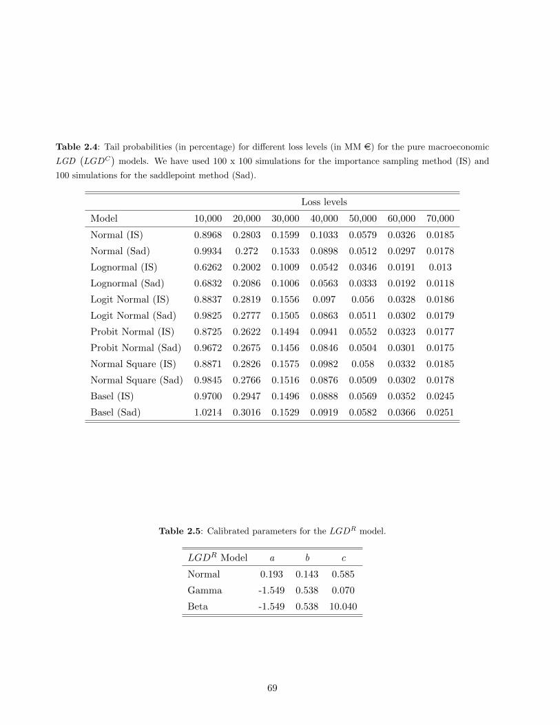
Table 2.4: Tail probabilities (in percentage) for different loss levels (in MM e) for the pure macroeconomic
LGD(LGDC
)models. We have used 100 x 100 simulations for the importance sampling method (IS) and
100 simulations for the saddlepoint method (Sad).
Loss levels
Model 10,000 20,000 30,000 40,000 50,000 60,000 70,000
Normal (IS) 0.8968 0.2803 0.1599 0.1033 0.0579 0.0326 0.0185
Normal (Sad) 0.9934 0.272 0.1533 0.0898 0.0512 0.0297 0.0178
Lognormal (IS) 0.6262 0.2002 0.1009 0.0542 0.0346 0.0191 0.013
Lognormal (Sad) 0.6832 0.2086 0.1006 0.0563 0.0333 0.0192 0.0118
Logit Normal (IS) 0.8837 0.2819 0.1556 0.097 0.056 0.0328 0.0186
Logit Normal (Sad) 0.9825 0.2777 0.1505 0.0863 0.0511 0.0302 0.0179
Probit Normal (IS) 0.8725 0.2622 0.1494 0.0941 0.0552 0.0323 0.0177
Probit Normal (Sad) 0.9672 0.2675 0.1456 0.0846 0.0504 0.0301 0.0175
Normal Square (IS) 0.8871 0.2826 0.1575 0.0982 0.058 0.0332 0.0185
Normal Square (Sad) 0.9845 0.2766 0.1516 0.0876 0.0509 0.0302 0.0178
Basel (IS) 0.9700 0.2947 0.1496 0.0888 0.0569 0.0352 0.0245
Basel (Sad) 1.0214 0.3016 0.1529 0.0919 0.0582 0.0366 0.0251
Table 2.5: Calibrated parameters for the LGDR model.
LGDR Model a b c
Normal 0.193 0.143 0.585
Gamma -1.549 0.538 0.070
Beta -1.549 0.538 10.040
69

Table 2.6: Tail probabilities (in percentage) for different loss levels (in MM e) for the mixed macroeconomic
and idiosyncratic random LGD(LGDR
)models. We have used 100 x 100 simulations for the importance
sampling (IS) method and 100 simulations for the Laplace inversion method (Lap).
Loss levels
Model 10,000 20,000 30,000 40,000 50,000 60,000 70,000
Normal (IS) 1.0061 0.2752 0.1429 0.0947 0.0612 0.0373 0.0246
Normal (Lap) 1.0492 0.2502 0.136 0.0838 0.0509 0.0335 0.0233
Gamma (IS) 1.074 0.3102 0.1395 0.0787 0.0479 0.0356 0.0266
Gamma (Lap) 1.0106 0.3242 0.1454 0.0857 0.0572 0.0386 0.0287
Beta (IS) 1.0296 0.3498 0.1583 0.0969 0.0633 0.0491 0.0376
Beta (Lap) 1.0203 0.3224 0.1424 0.0811 0.0529 0.0357 0.0242
Table 2.7: Discount factors by rating grade based on the average CDS spread and 3-year average maturity.
Investment Grade
Rating AAA AA+ AA AA- A+ A A- BBB+ BBB BBB-
Discount Factor 98.71% 98.69% 98.6% 98.37% 97.93% 97.14% 96.96% 96.63% 96.02% 95.94%
Speculative Grade
Rating BB+ BB BB- B+ B B- CCC/C
Discount Factor 95.79% 95.51% 94.99% 94.04% 92.33% 89.26% 83.93%
Table 2.8: Average 1-year rating migration matrix from S&P (2010).
AAA AA+ AA AA- A+ A A- BBB+ BBB BBB- BB+ BB BB- B+ B B- CCC/C D
AAA 91% 4% 3% 1% 0% 0% 0% 0% 0% 0% 0% 0% 0% 0% 0% 0% 0% 0.0249%
AA+ 2% 79% 12% 4% 1% 1% 0% 0% 0% 0% 0% 0% 0% 0% 0% 0% 0% 0.0253%
AA 1% 1% 84% 8% 3% 1% 0% 0% 0% 0% 0% 0% 0% 0% 0% 0% 0% 0.027%
AA- 0% 0% 5% 80% 10% 3% 1% 0% 0% 0% 0% 0% 0% 0% 0% 0% 0% 0.03%
A+ 0% 0% 1% 5% 81% 9% 3% 1% 0% 0% 0% 0% 0% 0% 0% 0% 0% 0.0356%
A 0% 0% 0% 1% 5% 81% 7% 3% 1% 0% 0% 0% 0% 0% 0% 0% 0% 0.0459%
A- 0% 0% 0% 0% 1% 7% 79% 8% 3% 1% 0% 0% 0% 0% 0% 0% 0% 0.0651%
BBB+ 0% 0% 0% 0% 0% 1% 7% 78% 9% 2% 0% 0% 0% 0% 0% 0% 0% 0.1005%
BBB 0% 0% 0% 0% 0% 1% 1% 7% 80% 6% 2% 1% 0% 0% 0% 0% 0% 0.1659%
BBB- 0% 0% 0% 0% 0% 0% 0% 2% 9% 76% 6% 3% 1% 1% 0% 0% 0% 0.2871%
BB+ 0% 0% 0% 0% 0% 0% 0% 1% 2% 13% 69% 7% 4% 1% 1% 0% 1% 0.5112%
BB 0% 0% 0% 0% 0% 0% 0% 0% 1% 3% 9% 71% 9% 3% 2% 1% 1% 0.9257%
BB- 0% 0% 0% 0% 0% 0% 0% 0% 0% 1% 2% 9% 71% 9% 4% 1% 1% 1.6925%
B+ 0% 0% 0% 0% 0% 0% 0% 0% 0% 0% 0% 2% 7% 73% 9% 3% 2% 3.111%
B 0% 0% 0% 0% 0% 0% 0% 0% 0% 0% 0% 0% 2% 9% 66% 9% 7% 5.735%
B- 0% 0% 0% 0% 0% 0% 0% 0% 0% 0% 0% 0% 1% 3% 10% 60% 14% 10.5892%
CCC/C 0% 0% 0% 0% 0% 0% 0% 0% 0% 0% 0% 0% 1% 2% 3% 11% 63% 19.5689%
70

Appendix of Figures
0 1 2 3 4 5 6 7 8
x 104
10−6
10−5
10−4
10−3
10−2
10−1
100
Loss (MM )
Tai
l pro
babi
lity
Loss Distribution
Sad 1,000MC 1,000,000IS 1,000 x 100
Figure 2.1: Loss distribution of the Spanish portfolio. We use the saddlepoint method (Sad) with 1,000
simulations, Monte Carlo (MC) with 1,000,000 simulations, and the importance sampling method (IS) with
1,000 x 100 simulations. The red circles indicate the saddlepoint estimates. The black and blue lines show,
respectively, the Monte Carlo and IS results and their 5%-95% confidence intervals (dashed lines).
0 1 2 3 4 5 6 7 8
x 104
10−6
10−5
10−4
10−3
10−2
10−1
100
Loss (MM )
Tai
l pro
babi
lity
Loss Distribution
Sad 1,000MC 1,000,000IS 1,000 x 100
2.7 2.8 2.9 3 3.1 3.2 3.3 3.4 3.5 3.6
x 104
10−3
Loss (MM )
Tai
l pro
babi
lity
Loss Distribution
Sad 1,000MC 1,000,000IS 1,000 x 100
Figure 2.2: Loss distribution of the Spanish portfolio considering the adaptative saddlepoint approximation.
Left and right graphs show, respectively, the tail distribution and the detail of the distribution in the neigh-
borhood of the 99.9% probability loss level. We use the saddlepoint method (Sad) with 1,000 simulations,
Monte Carlo (MC) with 1,000,000 simulations, and the importance sampling method (IS) with 1,000 x 100
simulations. The red circles indicate the saddlepoint estimates. The black and blue lines show, respectively,
the Monte Carlo and IS results and their 5%-95% confidence intervals (dashed lines).
71

0
10
20
30
40
50
60
70
80
%
VaR Based Risk Allocation
SANTANDER
BBVA
BANKIA
LA C
AIXA
POPULAR
SABADELL
CATALUNYACAIX
ANCG
BANCA CIV
ICACAM
MARE N
OST.
BANKINTER, S
ABASE
CAJA E
SPAÑABBK
IBERCAJA
UNICAJA
BARCLAYS
BANCO PASTOR
UNIMM
CAJAM
AR
BANCO DE V
ALENCIA
CAJA L
ABORAL
KUTXA
CAJA 3
Sad 100Sad−Mar 100Sad−Her 100
MC 106
IS 100x100
0
5
10
15
20
25
30
%
ES Based Risk Allocation
SANTANDER
BBVA
BANKIA
LA C
AIXA
POPULAR
SABADELL
CATALUNYACAIX
ANCG
BANCA CIV
ICACAM
MARE N
OST.
BANKINTER, S
ABASE
CAJA E
SPAÑABBK
IBERCAJA
UNICAJA
BARCLAYS
BANCO PASTOR
UNIMM
CAJAM
AR
BANCO DE V
ALENCIA
CAJA L
ABORAL
KUTXA
CAJA 3
Sad 100Sad−Her 100
MC 106
IS 100x100
Figure 2.3: Risk allocation. Left and right graphs show, respectively, the risk allocations based on the
VaR and the ES. We use the pure saddlepoint method (Sad), the saddlepoint based Martin approximation
(Sad-Mar), and the Hermite polynomials based saddlepoint approximation (Sad-Her) with 100 simulations,
Monte Carlo (MC) with 1,000,000 simulations, and the importance sampling method (IS) with 100 x 100
simulations.
0
10
20
30
40
50
60
70
80
%
VaR Based Risk Allocation
SANTANDER
BBVA
BANKIA
LA C
AIXA
POPULAR
SABADELL
CATALUNYACAIX
ANCG
BANCA CIV
ICACAM
MARE N
OST.
BANKINTER, S
ABASE
CAJA E
SPAÑABBK
IBERCAJA
UNICAJA
BARCLAYS
BANCO PASTOR
UNIMM
CAJAM
AR
BANCO DE V
ALENCIA
CAJA L
ABORAL
KUTXA
CAJA 3
Sad 1,000Sad−Mar 1,000Sad−Her 1,000
MC 106
IS 1,000x100
0
5
10
15
20
25
30
%
ES Based Risk Allocation
SANTANDER
BBVA
BANKIA
LA C
AIXA
POPULAR
SABADELL
CATALUNYACAIX
ANCG
BANCA CIV
ICACAM
MARE N
OST.
BANKINTER, S
ABASE
CAJA E
SPAÑABBK
IBERCAJA
UNICAJA
BARCLAYS
BANCO PASTOR
UNIMM
CAJAM
AR
BANCO DE V
ALENCIA
CAJA L
ABORAL
KUTXA
CAJA 3
Sad 1,000Sad−Her 1,000
MC 106
IS 1,000x100
Figure 2.4: Risk allocation. Left and right graphs show, respectively, the risk allocations based on the
VaR and the ES. We use the pure saddlepoint method (Sad), the saddlepoint based Martin approximation
(Sad-Mar), and the Hermite polynomials based saddlepoint approximation (Sad-Her) with 1,000 simulations,
Monte Carlo (MC) with 1,000,000 simulations, and the importance sampling method (IS) with 1,000 x 100
simulations.
72

0
10
20
30
40
50
60
%
VaR Allocation Normal LGD
SANTANDER
BBVA
BANKIA
LA C
AIXA
POPULAR
SABADELL
CATALUNYACAIX
ANCG
BANCA CIV
ICACAM
MARE N
OST.
BANKINTER, S
ABASE
CAJA E
SPAÑABBK
IBERCAJA
UNICAJA
BARCLAYS
BANCO PASTOR
UNIMM
CAJAM
AR
BANCO DE V
ALENCIA
CAJA L
ABORAL
KUTXA
CAJA 3
Sad 1,000Sad−Her 1,000IS 1,000x1,000
0
5
10
15
20
25
30
35
40
%
ES Allocation Normal LGD
SANTANDER
BBVA
BANKIA
LA C
AIXA
POPULAR
SABADELL
CATALUNYACAIX
ANCG
BANCA CIV
ICACAM
MARE N
OST.
BANKINTER, S
ABASE
CAJA E
SPAÑABBK
IBERCAJA
UNICAJA
BARCLAYS
BANCO PASTOR
UNIMM
CAJAM
AR
BANCO DE V
ALENCIA
CAJA L
ABORAL
KUTXA
CAJA 3
Sad 1,000Sad−Her 1,000IS 1,000x1,000
Figure 2.5: Risk Allocation Normal Macroeconomic LGD. We use the pure saddlepoint method (Sad) and the
Hermite polynomials based saddlepoint approximation (Sad-Her) with 1,000 simulations and the importance
sampling method (IS) with 1,000 x 1,000 simulations.
0
10
20
30
40
50
60
%
VaR Allocation Lognormal LGD
SANTANDER
BBVA
BANKIA
LA C
AIXA
POPULAR
SABADELL
CATALUNYACAIX
ANCG
BANCA CIV
ICACAM
MARE N
OST.
BANKINTER, S
ABASE
CAJA E
SPAÑABBK
IBERCAJA
UNICAJA
BARCLAYS
BANCO PASTOR
UNIMM
CAJAM
AR
BANCO DE V
ALENCIA
CAJA L
ABORAL
KUTXA
CAJA 3
Sad 1,000Sad−Her 1,000IS 1,000x1,000
0
5
10
15
20
25
30
35
40
%
ES Allocation Lognormal LGD
SANTANDER
BBVA
BANKIA
LA C
AIXA
POPULAR
SABADELL
CATALUNYACAIX
ANCG
BANCA CIV
ICACAM
MARE N
OST.
BANKINTER, S
ABASE
CAJA E
SPAÑABBK
IBERCAJA
UNICAJA
BARCLAYS
BANCO PASTOR
UNIMM
CAJAM
AR
BANCO DE V
ALENCIA
CAJA L
ABORAL
KUTXA
CAJA 3
Sad 1,000Sad−Her 1,000IS 1,000x1,000
Figure 2.6: Risk Allocation Lognormal Macroeconomic LGD. We use the pure saddlepoint method (Sad)
and the Hermite polynomials based saddlepoint approximation (Sad-Her) with 1,000 simulations and the
importance sampling method (IS) with 1,000 x 1,000 simulations.
73

0
10
20
30
40
50
60
%
VaR Allocation Logit Normal LGD
SANTANDER
BBVA
BANKIA
LA C
AIXA
POPULAR
SABADELL
CATALUNYACAIX
ANCG
BANCA CIV
ICACAM
MARE N
OST.
BANKINTER, S
ABASE
CAJA E
SPAÑABBK
IBERCAJA
UNICAJA
BARCLAYS
BANCO PASTOR
UNIMM
CAJAM
AR
BANCO DE V
ALENCIA
CAJA L
ABORAL
KUTXA
CAJA 3
Sad 1,000Sad−Her 1,000IS 1,000x1,000
0
5
10
15
20
25
30
35
40
%
ES Allocation Logit Normal LGD
SANTANDER
BBVA
BANKIA
LA C
AIXA
POPULAR
SABADELL
CATALUNYACAIX
ANCG
BANCA CIV
ICACAM
MARE N
OST.
BANKINTER, S
ABASE
CAJA E
SPAÑABBK
IBERCAJA
UNICAJA
BARCLAYS
BANCO PASTOR
UNIMM
CAJAM
AR
BANCO DE V
ALENCIA
CAJA L
ABORAL
KUTXA
CAJA 3
Sad 1,000Sad−Her 1,000IS 1,000x1,000
Figure 2.7: Risk Allocation Logit Normal Macroeconomic LGD. We use the pure saddlepoint method (Sad)
and the Hermite polynomials based saddlepoint approximation (Sad-Her) with 1,000 simulations and the
importance sampling method (IS) with 1,000 x 1,000 simulations.
0
10
20
30
40
50
60
%
VaR Allocation Probit Normal LGD
SANTANDER
BBVA
BANKIA
LA C
AIXA
POPULAR
SABADELL
CATALUNYACAIX
ANCG
BANCA CIV
ICACAM
MARE N
OST.
BANKINTER, S
ABASE
CAJA E
SPAÑABBK
IBERCAJA
UNICAJA
BARCLAYS
BANCO PASTOR
UNIMM
CAJAM
AR
BANCO DE V
ALENCIA
CAJA L
ABORAL
KUTXA
CAJA 3
Sad 1,000Sad−Her 1,000IS 1,000x1,000
0
5
10
15
20
25
30
35
40
%
ES Allocation Probit Normal LGD
SANTANDER
BBVA
BANKIA
LA C
AIXA
POPULAR
SABADELL
CATALUNYACAIX
ANCG
BANCA CIV
ICACAM
MARE N
OST.
BANKINTER, S
ABASE
CAJA E
SPAÑABBK
IBERCAJA
UNICAJA
BARCLAYS
BANCO PASTOR
UNIMM
CAJAM
AR
BANCO DE V
ALENCIA
CAJA L
ABORAL
KUTXA
CAJA 3
Sad 1,000Sad−Her 1,000IS 1,000x1,000
Figure 2.8: Risk Allocation Probit Normal Macroeconomic LGD. We use the pure saddlepoint method
(Sad) and the Hermite polynomials based saddlepoint approximation (Sad-Her) with 1,000 simulations and
the importance sampling method (IS) with 1,000 x 1,000 simulations.
74

0
10
20
30
40
50
60
%
VaR Allocation Normal Square LGD
SANTANDER
BBVA
BANKIA
LA C
AIXA
POPULAR
SABADELL
CATALUNYACAIX
ANCG
BANCA CIV
ICACAM
MARE N
OST.
BANKINTER, S
ABASE
CAJA E
SPAÑABBK
IBERCAJA
UNICAJA
BARCLAYS
BANCO PASTOR
UNIMM
CAJAM
AR
BANCO DE V
ALENCIA
CAJA L
ABORAL
KUTXA
CAJA 3
Sad 1,000Sad−Her 1,000IS 1,000x1,000
0
5
10
15
20
25
30
35
40
%
ES Allocation Normal Square LGD
SANTANDER
BBVA
BANKIA
LA C
AIXA
POPULAR
SABADELL
CATALUNYACAIX
ANCG
BANCA CIV
ICACAM
MARE N
OST.
BANKINTER, S
ABASE
CAJA E
SPAÑABBK
IBERCAJA
UNICAJA
BARCLAYS
BANCO PASTOR
UNIMM
CAJAM
AR
BANCO DE V
ALENCIA
CAJA L
ABORAL
KUTXA
CAJA 3
Sad 1,000Sad−Her 1,000IS 1,000x1,000
Figure 2.9: Risk Allocation Normal Square Macroeconomic LGD. We use the pure saddlepoint method
(Sad) and the Hermite polynomials based saddlepoint approximation (Sad-Her) with 1,000 simulations and
the importance sampling method (IS) with 1,000 x 1,000 simulations.
0
10
20
30
40
50
60
%
VaR Allocation Basel LGD
SANTANDER
BBVA
BANKIA
LA C
AIXA
POPULAR
SABADELL
CATALUNYACAIX
ANCG
BANCA CIV
ICACAM
MARE N
OST.
BANKINTER, S
ABASE
CAJA E
SPAÑABBK
IBERCAJA
UNICAJA
BARCLAYS
BANCO PASTOR
UNIMM
CAJAM
AR
BANCO DE V
ALENCIA
CAJA L
ABORAL
KUTXA
CAJA 3
Sad 1,000Sad−Her 1,000IS 1,000x1,000
0
5
10
15
20
25
30
35
40
%
ES Allocation Basel LGD
SANTANDER
BBVA
BANKIA
LA C
AIXA
POPULAR
SABADELL
CATALUNYACAIX
ANCG
BANCA CIV
ICACAM
MARE N
OST.
BANKINTER, S
ABASE
CAJA E
SPAÑABBK
IBERCAJA
UNICAJA
BARCLAYS
BANCO PASTOR
UNIMM
CAJAM
AR
BANCO DE V
ALENCIA
CAJA L
ABORAL
KUTXA
CAJA 3
Sad 1,000Sad−Her 1,000IS 1,000x1,000
Figure 2.10: Risk Allocation Basel Macroeconomic LGD. We use the pure saddlepoint method (Sad) and the
Hermite polynomials based saddlepoint approximation (Sad-Her) with 1,000 simulations and the importance
sampling method (IS) with 1,000 x 1,000 simulations.
75
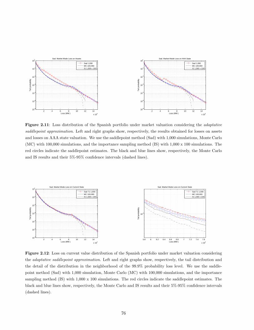
2 4 6 8 10 12 14
x 104
10−6
10−5
10−4
10−3
10−2
10−1
100
Loss (MM )
Tai
l pro
babi
lity
Sad. Market Mode Loss on Assets
Sad 1,000MC 100,000IS 1,000 x 100
2 4 6 8 10 12 14
x 104
10−6
10−5
10−4
10−3
10−2
10−1
100
Loss (MM )
Tai
l pro
babi
lity
Sad. Market Mode Loss on AAA State
Sad 1,000MC 100,000IS 1,000 x 100
Figure 2.11: Loss distribution of the Spanish portfolio under market valuation considering the adaptative
saddlepoint approximation. Left and right graphs show, respectively, the results obtained for losses on assets
and losses on AAA state valuation. We use the saddlepoint method (Sad) with 1,000 simulations, Monte Carlo
(MC) with 100,000 simulations, and the importance sampling method (IS) with 1,000 x 100 simulations. The
red circles indicate the saddlepoint estimates. The black and blue lines show, respectively, the Monte Carlo
and IS results and their 5%-95% confidence intervals (dashed lines).
2 4 6 8 10 12 14
x 104
10−6
10−5
10−4
10−3
10−2
10−1
100
Loss (MM )
Tai
l pro
babi
lity
Sad. Market Mode Loss on Current State
Sad T1 1,000MC 100,000IS 1,000 x 100
5.8 6 6.2 6.4 6.6 6.8 7 7.2 7.4 7.6
x 104
10−3
Loss (MM )
Tai
l pro
babi
lity
Sad. Market Mode Loss on Current State
Sad T1 1,000MC 100,000IS 1,000 x 100
Figure 2.12: Loss on current value distribution of the Spanish portfolio under market valuation considering
the adaptative saddlepoint approximation. Left and right graphs show, respectively, the tail distribution and
the detail of the distribution in the neighborhood of the 99.9% probability loss level. We use the saddle-
point method (Sad) with 1,000 simulation, Monte Carlo (MC) with 100,000 simulations, and the importance
sampling method (IS) with 1,000 x 100 simulations. The red circles indicate the saddlepoint estimates. The
black and blue lines show, respectively, the Monte Carlo and IS results and their 5%-95% confidence intervals
(dashed lines).
76

0
10
20
30
40
50
%
VaR Based Risk Allocation
SANTANDER
BBVA
BANKIA
LA C
AIXA
POPULAR
SABADELL
CATALUNYACAIX
ANCG
BANCA CIV
ICACAM
MARE N
OST.
BANKINTER, S
ABASE
CAJA E
SPAÑABBK
IBERCAJA
UNICAJA
BARCLAYS
BANCO PASTOR
UNIMM
CAJAM
AR
BANCO DE V
ALENCIA
CAJA L
ABORAL
KUTXA
CAJA 3
Sad 100Sad−Her 100IS 10,000x100
0
10
20
30
40
50
60
70
%
ES Based Risk Allocation
SANTANDER
BBVA
BANKIA
LA C
AIXA
POPULAR
SABADELL
CATALUNYACAIX
ANCG
BANCA CIV
ICACAM
MARE N
OST.
BANKINTER, S
ABASE
CAJA E
SPAÑABBK
IBERCAJA
UNICAJA
BARCLAYS
BANCO PASTOR
UNIMM
CAJAM
AR
BANCO DE V
ALENCIA
CAJA L
ABORAL
KUTXA
CAJA 3
Sad 100Sad−Her 100IS 10,000x100
Figure 2.13: VaR and ES contributions for the market mode model. Left and right graphs show, respectively,
the risk allocations based on the VaR and the ES. We use the pure saddlepoint method (Sad) and the Hermite
polynomials based saddlepoint approximation (Sad-Her) with 100 simulations and the importance sampling
method (IS) with 10,000 x 100 simulations.
0
0.2
0.4
0.6
0.8
1
%
VaR Based Risk Allocation
SANTANDER
BBVA
BANKIA
LA C
AIXA
POPULAR
SABADELL
CATALUNYACAIX
ANCG
BANCA CIV
ICACAM
MARE N
OST.
BANKINTER, S
ABASE
CAJA E
SPAÑABBK
IBERCAJA
UNICAJA
BARCLAYS
BANCO PASTOR
UNIMM
CAJAM
AR
BANCO DE V
ALENCIA
CAJA L
ABORAL
KUTXA
CAJA 3
Sad 100Sad−Her 100IS 10,000x100
0
0.2
0.4
0.6
0.8
1
%
ES Based Risk Allocation
SANTANDER
BBVA
BANKIA
LA C
AIXA
POPULAR
SABADELL
CATALUNYACAIX
ANCG
BANCA CIV
ICACAM
MARE N
OST.
BANKINTER, S
ABASE
CAJA E
SPAÑABBK
IBERCAJA
UNICAJA
BARCLAYS
BANCO PASTOR
UNIMM
CAJAM
AR
BANCO DE V
ALENCIA
CAJA L
ABORAL
KUTXA
CAJA 3
Sad 100Sad−Her 100IS 10,000x100
Figure 2.14: VaR and ES contributions on an equally weighted (EAD) portfolio for the market mode model.
Left and right graphs show, respectively, the risk allocations based on the VaR and the ES. We use the pure
saddlepoint method (Sad) and the Hermite polynomials based saddlepoint approximation (Sad-Her) with 100
simulations and the importance sampling method (IS) with 10,000 x 100 simulations.
77

Chapter 3
Taylor expansion based methods to measure credit risk
3.1 Introduction
This paper uses the Taylor expansion based method in Pykhtin (2004) to obtain an analytical
estimation of the credit risk loss distribution of the Spanish financial system. We compare the results
of the method with those obtained using Monte Carlo simulations. We also propose an approximate
method to calculate the loss distribution of a portfolio under random correlated recoveries. We
consider that this kind of approximations can be easily implemented under the Basel capital charge
regulation.
In previous papers (see Garcıa-Cespedes and Moreno (2014) and Garcıa-Cespedes and Moreno
(2014b)) we studied the loss distribution of the Spanish financial system using importance sampling
techniques and the saddlepoint methods, respectively. Both methods are subject to random variabil-
ity due to the Monte Carlo simulation, this noise is more intense in the risk allocation process. One
of the objectives of this paper is to analyze the suitability of the Taylor expansion based method to
measure the credit risk of a portfolio. In the Taylor expansion based method introduced in Pykhtin
(2004), the real loss distribution is approximated using the loss distribution of a similar portfolio
plus several adjustment terms. This type of expansion is related with the Taylor expansion of the
real loss distribution and the adjustment terms are related with the derivatives of the moments of
the portfolio loss.
This paper provides two major contributions to the literature. First, we use the approximation in
Pykhtin (2004) to measure the risk of the Spanish financial system portfolio built in Garcıa-Cespedes
and Moreno (2014) and we allocate it over the different financial institutions. To allocate the risk we
use some of the results in Morone et al. (2012). Second, we develop two simple correlated recoveries
models and we use the Taylor expansion ideas to approximate the loss distribution under random
correlated recoveries.
According to our results, the Pykhtin model does not perform well in the case of concentrated
78

portfolios, it is not able to capture the sudden jumps in the loss distribution, neither it is able to
properly allocate the risk over the counterparties. However we get very satisfactory results when we
apply the Taylor expansion ideas to approximate the loss distribution of a portfolio under random
and correlated recoveries.
This paper is organized as follows. Sections 2 and 3 introduce, respectively, the Vasicek (1987)
and the Pykhtin (2004) models. Section 4 describes the Spanish financial institutions portfolio and
obtains its loss distribution and risk allocation applying the Pykhtin (2004) model. In Section 5 we
develop two correlated recoveries models and use the Taylor expansion ideas to approximate the loss
distribution. Finally, Section 6 summarizes our main results and concludes.
3.2 The Vasicek (1987) model
We will start remembering the credit risk model developed in Vasicek (1987). This model states that
the value of a counterparty j, Vj , is driven by a own macroeconomic normal factor Yj and an idiosyn-
cratic independent normal term ξj . The own macroeconomic factor Yj is the linear combination of
some more general macroeconomic independent factors zf . Then we can write
Vj = rjYj +√
1− r2j ξj = rj
k∑f=1
αf,jzf +√
1− r2j ξj
=k∑
f=1
βf,jzf +
√√√√1−k∑
f=1
(βf,j)2 ξj (3.1)
The client j defaults in his obligations if the assets value Vj falls below a given level k. As
Vj ∼ N(0, 1) there exist a direct relation between the default threshold k and the historical average
default rates of client j, PDj,C (or over the cycle default rate), this is k = Φ−1(PDj,C), where Φ−1(·)denotes the inverse normal distribution. The total losses L of a portfolio made up of M clients can
be obtained adding the individual ones, that is,
L =
M∑j=1
xj(Yj , ξj) =
M∑j=1
EADjLGDjDj(Yj , ξj)
where Dj is a dummy variable that indicates if the clients defaults, EADj is the exposure at
default (the amount owed by the client j, or by the clients in the subportfolio j, in the default
moment), and LGDj is the loss given default (the percentage of the final loss after all the recovery
process relative to the exposure at default). For the sake of simplicity we will use the notation
EADjLGDj = gj .
79

Given the specification in (3.1) and conditional to the macroeconomic factors Z = z1, z2, · · · , zk,the default probability of the client j is
pj(Z) = Prob(Dj = 1|Z) = Prob(Vj ≤ k) = Prob
ξj ≤ k − rj∑k
f=1 αfzf√1− r2
j
= Φ
Φ−1(PDj,C)− rj∑k
f=1 αfzf√1− r2
j
In a granular portfolio (many identical clients) made up of M different subportfolios, the losses
conditional to a macroeconomic scenario are
L|z =
M∑j=1
gjΦ
Φ−1(PDj,C)− rj∑k
f=1 αfzf√1− r2
j
=
M∑j=1
gjpj(Z)
If all the clients in the portfolio are exposed to the same macroeconomic factor, the loss at a
given probability level q can be obtained just replacing z by Φ−1(q) in the previous formula. But in
the general case of multi-factor and non-granular portfolios, closed-form expressions are not available
and Monte Carlo methods or approximate formulas are needed.1
3.3 The Pykhtin (2004) approximate model
Given a certain confidence level q, Pykhtin (2004) suggests to estimate the value at risk (V aR(q))
and the expected shortfall (ES(q)) by approximating the loss distribution of the real portfolio
through a Taylor expansion. This author considers a granular and unifactorial portfolio as starting
point and then adds some adjustment terms to capture the non-granularity and the multifactoriality
of the real portfolio. Following Pykhtin (2004), we consider the random variable L and define
Lε = L+ εU, ε ∈ R, with U = L− L.2 Let tq(L) denote the percentile q of the random variable L.
Then, a Taylor expansion of tq(Lε=1) around ε = 0 leads to
tq(L) = tq(Lε=1) = tq(L) +dtq(Lε)
dε
∣∣∣∣ε=0
+1
2
d2tq(Lε)
dε2
∣∣∣∣ε=0
+ · · · (3.2)
Gourieroux et al. (2000) and Martin and Wilde (2002) provide an analytical expression for the
previous two derivatives
dtq(Lε)
dε
∣∣∣∣ε=0
= E(U |L = tq
(L))
(3.3)
d2tq(Lε)
dε2
∣∣∣∣ε=0
= − 1
fL(l)
d
dl
(fL(l)var
(U |L = l
))∣∣∣∣l=tq(L)
(3.4)
1See, for instance, Pykhtin (2004), Glasserman and Li (2005) or Voropaev (2011).2It is straightforward to see that Lε=1 = L.
80

where var() stands for the variance of a random variable. Pykhtin (2004) suggests to define L
as the losses of a granular and unifactorial portfolio that depends on a single macroeconomic factor
Y =∑k
f=1 bfzf where∑k
f=1 b2f = 1. Intuitively this unique macroeconomic factor should try to
capture most of the influence of the different zf on the losses of the real portfolio. Then, we have
L(Y ) =
M∑j=1
gjΦ
Φ−1(PDj,C)− ajY√1− a2
j
=
M∑j=1
gj pj(Y ) (3.5)
The terms aj are the sensitivities of the clients in the granular portfolio to the single macroeco-
nomic factor Y .3
According to the previous definitions of L and Y , we can rewrite the macroeconomic factor Yj
and the asset value of each client Vj as
Yj = Y
k∑f=1
αj,fbf +
√√√√√1−
k∑f=1
αj,fbf
2
γj
Vj = rjY
k∑f=1
αj,fbf +
√√√√√1−
rj k∑f=1
αj,fbf
2
ψj (3.6)
where the random variables γj and ψj are independent of Y but γj and γi are correlated between
clients, and so are ψj and ψi.
Now we can estimate E(L|L). Looking at equation (3.6), we have that
E(L|L
)= E
(L|Y
)=
M∑j=1
gjΦ
Φ−1(PDj,C)− rjY∑k
f=1 αj,fbf√1−
(rj∑k
f=1 αj,fbf
)2
(3.7)
Comparing equations (3.5) and (3.7) we can see that if we define aj = rj∑k
f=1 αj,fbf =∑kf=1 βj,fbf then equation (3.3) equals to zero and the first derivative term in the Taylor expan-
sion vanishes. It is also important to note that, given the previous definition of aj , we can rewrite
equation (3.6) in a much shorter way
Vj = ajY +√
1− a2j ψj (3.8)
Then, Vj conditional to Y is distributed as N(ajY ,
√1− a2
j
). The correlation between Vj and
Vi conditional to Y will be required later in order to obtain equation (3.4) and it is equal to that
between ψj and ψi. Using equations (3.1) and (3.8), we can get
E(ψjψi) =
∑kf=1 βf,jβf,i − aiaj√(1− a2
j )(1− a2i )
(3.9)
3In the next paragraphs we will show a criterion to set aj such that the first derivative in equation (3.2) vanishes.
81

On the other hand, Pykhtin (2004) suggests to set the coefficients bf that define the single
macroeconomic factor Y as
bf (q) =
∑Mj=1 αj,fgjpj(Yj)√∑k
f=1
(∑Mj=1 αj,fgjpj(Yj)
)2
∣∣∣∣∣∣∣∣Yj=Φ−1(q)
This is a weighted sum of the expected losses of every client in the portfolio given that each of
the own macroeconomic factors is in its q percentile.
To estimate the second derivative in equation (3.4) we first note that conditioning to L is the
same as conditioning to Y . As Y ∼ N(0, 1), we have φ′(y) = −yφ(y). Then, equation (3.4) becomes
d2tq(Lε)
dε2
∣∣∣∣ε=0
= − 1
φ(Y )
d
dY
(φ(Y )
L′(Y )
var(U |Y )
)∣∣∣∣∣Y=Φ−1(q)
=1
L′(Y )
(−v′(Y ) + v(Y )
(Y +
L′′(Y )
L′(Y )
))∣∣∣∣∣Y=Φ−1(q)
(3.10)
where v(Y ) = var(U |Y ). Equation (3.10) requires the following inputs
L′(Y ) = −
M∑j=1
gjaj√
1− a2j
φ
Φ−1(PDj,C)− ajY√1− a2
j
L′′(Y ) = −
M∑j=1
gja2j
1− a2j
Φ−1(PDj,C)− ajY√1− a2
j
φ
Φ−1(PDj,C)− ajY√1− a2
j
v(Y ) = var(U |Y ) = var(L|Y ) = var
M∑j=1
gjDj
∣∣∣∣∣∣Y
= E
M∑j=1
gjDj
2∣∣∣∣∣∣Y−
E M∑
j=1
gjDj
∣∣∣∣∣∣Y2
=
M∑j=1
M∑i=1
gjgiE(DiDj |Y
)−
E M∑
j=1
gjDj
∣∣∣∣∣∣Y2
=M∑j=1
M∑i 6=j
gjgiE(DiDj |Y
)+
M∑j=1
g2jE(Dj |Y
)−
M∑j=1
gjE(Dj |Y )
2
=M∑j=1
M∑i 6=j
gjgiΦ2
(Φ−1(pj(Y )),Φ−1(pi(Y )), ρi,j
)+
M∑j=1
g2j pj(Y )
−
M∑j=1
gj pj(Y )
2
(3.11)
82

where Φ2 (·, ·, ·) denotes the bivariate cumulative standard normal distribution and ρi,j is given
by equation (3.9). We explored different algorithms to implement this bivariate distribution4 and
obtained the best results in terms of accuracy, speed, and possibility to be vectorized using the
method proposed in Genz (2004).
Equation (3.10) also requires to compute the first derivative of v(Y ), v′(Y ). Setting Zj(Y ) =
Φ−1(pj(Y )) we have that Z ′j(Y ) =p′j(Y )
φ(Zj(Y ))and some algebra leads to
d
dY
[Φ2
(Zj(Y ), Zi(Y ), ρi,j
)]= p′j(Y )Φ
Zi(Y )− ρi,jZj(Y )√1− ρ2
i,j
+p′i(Y )Φ
Zj(Y )− ρi,jZi(Y )√1− ρ2
i,j
Therefore we get that
v′(Y ) = 2
M∑j=1
M∑i 6=j
gjgip′i(Y )Φ
Zj(Y )− ρi,jZi(Y )√1− ρ2
i,j
+
M∑j=1
g2j p′j(Y )
−2M∑j=1
gj pj(Y )M∑j=1
gj p′j(Y ) (3.12)
Pykhtin (2004) also obtains an analytical approximation for the expected shortfall (ES) given by
ESq(L) =1
1− q
∫ 1
qts(L)ds =
1
1− q
∫ 1
q[ts(L) + ∆ts(L)]ds
= ESq(L) +1
1− q
∫ 1
q∆ts(L)ds = ESq(L) + ∆ESq(L)
where
ESq(L) =1
1− q
∫ Φ−1(1−q)
−∞L(Y )φ(Y )dY
=1
1− q
M∑j=1
gjΦ2
(Φ−1 (PDj,C) ,Φ−1(1− q), aj
)∆ESq(L) = − 1
2(1− q)
∫ Φ−1(1−q)
−∞
1
φ(Y) d
dY
(φ(Y)
L′ (Y)v (Y ))φ(Y )dY
= −v(Y)
2(1− q)φ(Y)
L′ (Y)∣∣∣∣∣Y=Φ−1(1−q)
4See Chance and Agca (2003) for a general review of these alternatives or Owen (1956), Vasicek (1996), Genz
(2004), and Hull (2011) for a more detailed explanation.
83

As it can be observed all the information required to obtain the expected shortfall has been
obtained previously to estimate the VaR, this is a big advantage of this method.
Now let us focus on two extreme cases:
1. For a single factor and non-granular portfolio, we have ρi,j = 0 and equations (3.11)-(3.12)
simplify to
v(Y)
=
M∑j=1
M∑i 6=j
gjgipj(Y)pi(Y)
+
M∑j=1
g2j pj(Y)−
M∑j=1
gj pj(Y)2
v′(Y)
= 2
M∑j=1
M∑i 6=j
gjgip′i
(Y)pj(Y)
+
M∑j=1
g2j p′j
(Y)
−2
M∑j=1
gj pj(Y) M∑j=1
gj p′j
(Y)
2. In the case of multifactorial and granular portfolio, equations (3.11)-(3.12) simplify to
v(Y)
=M∑j=1
M∑i=1
gjgiΦ2
(Φ−1(pj
(Y)),Φ−1(pi
(Y)), ρi,j
)−
M∑j=1
M∑i=1
gjgipi(Y)pj(Y )
v′(Y)
= 2
M∑j=1
M∑i=1
gjgip′i
(Y)Φ
Zj (Y )− ρi,jZi (Y )√1− ρ2
i,j
− pj (Y )
3.4 Portfolio Results
We study the portfolio of financial institutions covered by the Spanish deposit guaranty fund (FGD)
at December, 2010. To obtain the risk measures of the portfolio first we need to have an estimate
of the probability of default (PD), exposure at default (EAD), loss given default (LGD) and the
macroeconomic factor sensitivity (α) of each institution.
We estimate the EAD based on the information on assets and liabilities for the Spanish financial
institutions at December 2010. This information can be obtained from the AEB, CECA, and AECR
webpages.5 During year 2010 many mergers took place, therefore we sum all the balance information
from the different institutions that belong to the same group.
For the PD we use the public credit ratings available at December 2010 and the historical
observed default rates reported by the rating agencies (see S&P (2009), Moody’s (2009) and Fitch
5AEB is the Spanish Bank Association, CECA is the Spanish Saving Bank Association, and AECR is the Spanish
Credit Cooperatives Association.
84

(2009)). Based on those data we infer a default probability for each institution. For those financial
institutions with no external rating we assign one notch less than the average rating of the portfolio
of financial institutions with external rating.
We extend the LGD results for financial institutions in Bennet (2002) to the period 1986-2009
using the FDIC (deposits guarantee fund in United States) public data of default recoveries.
The macroeconomic factor sensitivity, α, is set as the one in the Basel accord. Additionally all
the financial institutions in the portfolio are exposed to a single macroeconomic factor, the Spanish
factor. This is the case for all the institutions but for BBVA and Santander that are exposed to
additional geographies. The exposure of those two institutions to the geographic factors is computed
according to their net interest income by geography obtained from the public 2010 annual reports.
As we have more than one macroeconomic factor we need a factor correlation matrix, we obtain this
matrix using the GDP series of the different countries. Finally we compute orthogonalized factors
so that we can apply Pykhtin model.
3.4.1 Portfolio VaR and ES
We have tested the accuracy of the approximate formulas in Pykhtin (2004) using the portfolio of the
Spanish financial system at December 2010. The left graph in Figure 3.1 shows the loss distribution
obtained using a simple Monte Carlo method (MC) and the Pykhtin approximation. We show the
results of the Pykhtin model when only the first term or the first two terms of the approximation
are considered (Pykhtin 1, Pykhtin 2). It can be seen that the Pykhtin method underestimates the
probability of high losses for our portfolio. Another issue to be noted is that this method generates
an approximation of the percentiles of the loss distribution which is smooth (continuous derivatives)
and can not capture the sudden jumps of the portfolio loss distribution.
[INSERT FIGURE 3.1 AROUND HERE]
The right graph in Figure 3.1 provides the expected shortfall estimates using the Pykhtin (2004)
method (Pykhtin 1, 2) and the exact ones obtained using the Monte Carlo method (MC). The
conclusions are similar to those obtained from the loss distribution approximation.
3.4.2 Analytical VaR Contributions
The VaR contribution of a client i can be defined as the derivative of the VaR with respect to the
current exposure share of the client i, this is
CV aRi =∂V aR(w1, · · · , wm)
∂wi
∣∣∣∣wi=1
(3.13)
85

where the portfolio loss is defined as L =∑M
j=1[wjEADj ]LGDjDj . Under the Pykhtin approx-
imation approach, we need to obtain the derivative of (3.2) with respect to wi. This can be done
numerically by computing the values tq (L,w1, · · · , wi, · · · , wM ) and tq (L,w1, · · · , wi + λ, · · · , wM )
with λ being small enough and using these values to approximate the derivative in equation (3.13).
Unfortunately, this method must be repeated for all the clients as the information used to obtain
the derivative of the client j can not be used for another client with the corresponding lack of
computational synergies.
Alternatively, we can try to derivate equation (3.2) analytically. However, this derivative involves
those of aj(w1, · · · , wi, · · · , wM ) with respect to wi and this increases the complexity of the analytical
derivation. This derivation is considerably simplified if we assume aj(w1, · · · , wi, · · · , wM ) to be
constant, a (naive) case considered in Morone et al. (2012). We will obtain the terms of the analytical
approximation of the VaR contributions under this assumption and will compare the results against
a numerical derivation rule and against a Monte Carlo risk allocation rule. The analytical derivation
rule has a big computational advantage, namely, most of the terms required in the derivation process
have already being obtained for the VaR calculation.
Therefore, the VaR contribution of the client i can be obtained as
CV aRi ≈∂tq(L)
∂wi
∣∣∣∣wi=1
+∂
2∂wi
(d2tq(Lε)
dε2
∣∣∣∣ε=0
)∣∣∣∣wi=1
(3.14)
Under the assumption that aj(w1, · · · , wi, · · · , wM ) is constant, obtaining the first term of the
right-hand side of this equation is straightforward considering equation (3.5). Looking at (3.10), the
second term in equation (3.14) is given by
1
2(L′(Y ))2
×
[−L′(Y )
∂v′(Y )
∂wi+ v′(Y )
∂L′(Y )
∂wi
+
(Y +
L′′(Y )
L′(Y )
)(L′(Y )
∂v(Y )
∂wi− v(Y )
∂L′(Y )
∂wi
)
+ v(Y )L(Y )∂
∂wi
(Y +
L′′(Y )
L′(Y )
)]∣∣∣∣∣Y=Φ−1(1−q),wi=1
where
86

∂L′(Y )
∂wi
∣∣∣∣∣wi=1
= gip′i(Y )
∂L′′(Y )
∂wi
∣∣∣∣∣wi=1
= gip′′i (Y )
∂v(Y )
∂wi
∣∣∣∣wi=1
= 2∑j 6=i
gjgiΦ2
(Φ−1(pj(Y )),Φ−1(pi(Y )), ρi,j
)+ 2g2
i pi(Y )
−2gipi(Y )M∑j=1
gj pj(Y )
∂v′(Y )
∂wi
∣∣∣∣wi=1
= 2∑j 6=i
gigj p′i(Y )Φ
Zj(Y )− ρi,jZi(Y )√1− ρ2
i,j
+2∑j 6=i
gigj p′j(Y )Φ
Zi(Y )− ρi,jZj(Y )√1− ρ2
i,j
+2g2
i p′i(Y )− 2gipi(Y )
M∑j=1
gj p′j(Y )− 2gip
′i(Y )
M∑j=1
gj pj(Y )
The left graph in Figure 3.2 shows the loss allocation of the 99.9% probability loss level6 based
on the VaR contribution. We show the results for the risk allocation using Monte Carlo method
(MC) and three alternatives in the Pykhtin approximation derivatives: analytical derivation formula
(Pykthin Anal), and two types of numerical derivatives, one that varies the values of aj and bf as
λ varies on the derivation process (Pykthin Num. Der.) and another one that maintains them
constant (Pykthin Num. Der. Const.). It can be seen that the results from the analytical derivation
rule coincide with those from the numerical derivation rules. We also observe that the Pykhtin rule
based method does not provide accurate results for our portfolio. This is obvious for BBVA and
Santander as their contributions should be zero.
[INSERT FIGURE 3.2 AROUND HERE]
In the case of the expected shortfall we have a similar formula
CESi =∂ES(w1, · · · , wm)
∂wi
∣∣∣∣wi=1
≈ gi1− q
Φ2
(Φ−1(PDi,C),Φ−1(1− q), ai
)− φ(Y )
2(1− q)(L′(Y ))2
[∂v(Y )
∂wiL′(Y )− ∂L
′(Y )
∂wiv(Y )
]625,645 MMe and 31,053 MMe for the Pykhtin approximation and the Monte Carlo method, respectively.
87

The results for the expected shortfall based risk allocation can be observed in the right graph in
Figure 3.2. We can see that the results obtained using the Pykhtin approximation are quite close to
those provided by the Monte Carlo method.
We finish here our study of the Taylor expansions for the Vasicek (1987) model. An obvious
further research is to extend the Pykhtin model for the case of market valuation. In this case, the
different clients in a portfolio can migrate to several discrete states (not only to the default one) and,
on each state, the loans have a different valuation or loss. Therefore, the estimation of v(y) requires
to consider all the possible combinations of states of clients i and j. This problem is quadratic
in the number of clients and in the number of states. For instance, considering 156 clients and a
rating scale with 17 grades, we must estimate 156 x 156 x 17 x 17 bivariate cumulative standard
normal probabilities. This makes the utilization of the Pykhtin method less interesting in the case
of market valuation. In the next Section we will apply the Taylor expansion ideas to approximate
the loss distribution in the case of random recoveries in the Vasicek (1987) model.
3.5 Correlated random LGD
So far we have introduced the Taylor approximation method proposed in Pykhtin (2004) and used
it to estimate the loss distribution of the portfolio of Spanish financial institutions and its risk
contributions. We believe that this Taylor based approximation can be also used to approximate
the case of random correlated recoveries. In the next sections we will introduce a simple model of
random LGD and use the Taylor expansion ideas to approximate a more general model.
3.5.1 Simple random LGD model
We have developed a very simple random LGD model based on a single macroeconomic factor z
that drives both default and recoveries in a granular portfolio. To keep it simple we assume that the
recoveries follow a Bernoulli random variable that takes the values 0, 1 depending on the value of
the random variable Vj,LGD. According to this we have that
L =M∑j=1
xj =M∑j=1
gj DPD,j (Vj,PD) DLGD,j (Vj,LGD)
Each client has a default value function (Vj,PD) and a LGD value function (Vj,LGD) given by
Vj,PD = ρj,PDz + εj
√1− ρ2
j,PD
Vj,LGD = ρj,LGDz + ψj
√1− ρ2
j,LGD
As usual, if Vj,PD < Φ−1(PDj,C), the client defaults but now we also have that if Vj,LGD <
Φ−1(LGDj,C) the LGD is 100%. Conditional to a macroeconomic scenario, the loss distribution of
88
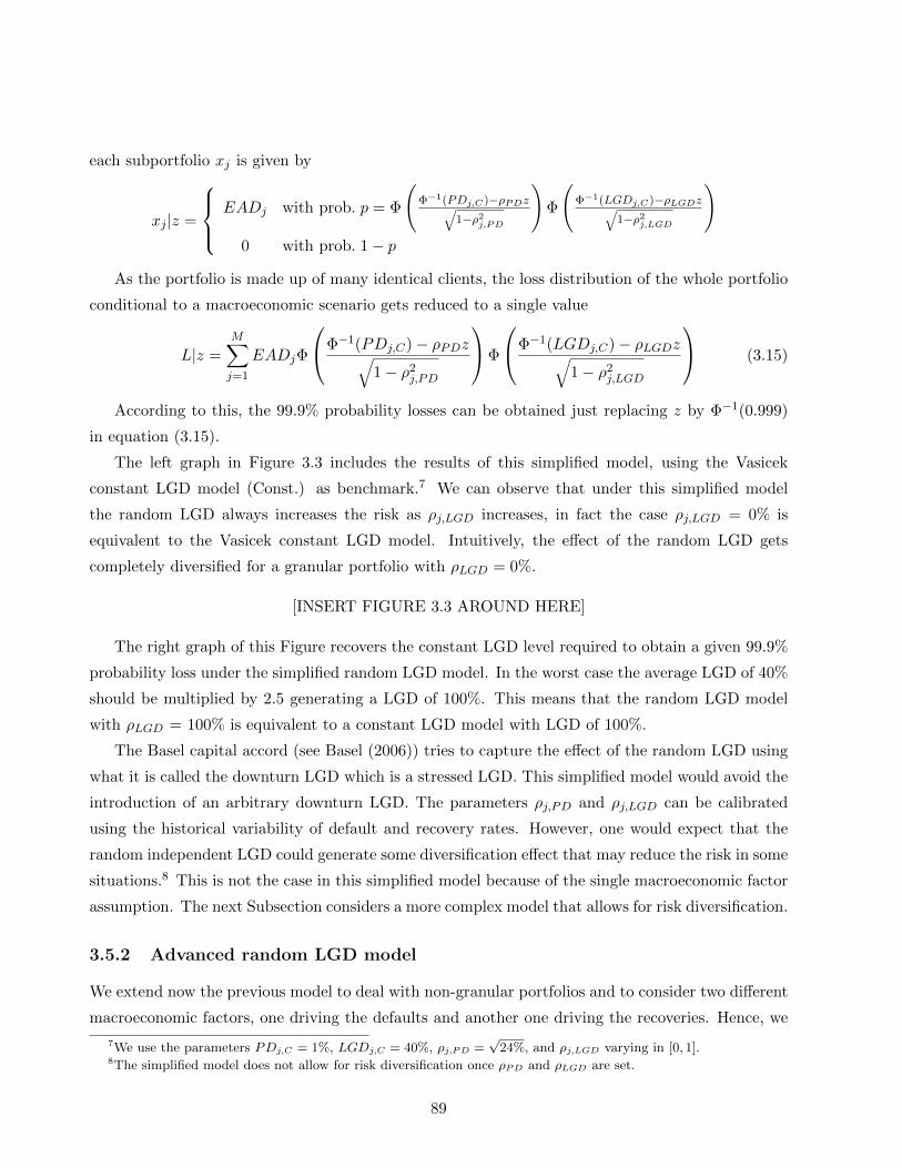
each subportfolio xj is given by
xj |z =
EADj with prob. p = Φ
(Φ−1(PDj,C)−ρPDz√
1−ρ2j,PD
)Φ
(Φ−1(LGDj,C)−ρLGDz√
1−ρ2j,LGD
)0 with prob. 1− p
As the portfolio is made up of many identical clients, the loss distribution of the whole portfolio
conditional to a macroeconomic scenario gets reduced to a single value
L|z =M∑j=1
EADjΦ
Φ−1(PDj,C)− ρPDz√1− ρ2
j,PD
Φ
Φ−1(LGDj,C)− ρLGDz√1− ρ2
j,LGD
(3.15)
According to this, the 99.9% probability losses can be obtained just replacing z by Φ−1(0.999)
in equation (3.15).
The left graph in Figure 3.3 includes the results of this simplified model, using the Vasicek
constant LGD model (Const.) as benchmark.7 We can observe that under this simplified model
the random LGD always increases the risk as ρj,LGD increases, in fact the case ρj,LGD = 0% is
equivalent to the Vasicek constant LGD model. Intuitively, the effect of the random LGD gets
completely diversified for a granular portfolio with ρLGD = 0%.
[INSERT FIGURE 3.3 AROUND HERE]
The right graph of this Figure recovers the constant LGD level required to obtain a given 99.9%
probability loss under the simplified random LGD model. In the worst case the average LGD of 40%
should be multiplied by 2.5 generating a LGD of 100%. This means that the random LGD model
with ρLGD = 100% is equivalent to a constant LGD model with LGD of 100%.
The Basel capital accord (see Basel (2006)) tries to capture the effect of the random LGD using
what it is called the downturn LGD which is a stressed LGD. This simplified model would avoid the
introduction of an arbitrary downturn LGD. The parameters ρj,PD and ρj,LGD can be calibrated
using the historical variability of default and recovery rates. However, one would expect that the
random independent LGD could generate some diversification effect that may reduce the risk in some
situations.8 This is not the case in this simplified model because of the single macroeconomic factor
assumption. The next Subsection considers a more complex model that allows for risk diversification.
3.5.2 Advanced random LGD model
We extend now the previous model to deal with non-granular portfolios and to consider two different
macroeconomic factors, one driving the defaults and another one driving the recoveries. Hence, we
7We use the parameters PDj,C = 1%, LGDj,C = 40%, ρj,PD =√
24%, and ρj,LGD varying in [0, 1].8The simplified model does not allow for risk diversification once ρPD and ρLGD are set.
89

have
Vj,PD = ρj,PD zPD + εj
√1− ρ2
j,PD
Vj,LGD = ρj,LGD zLGD + ψj
√1− ρ2
j,LGD
where the macroeconomic factors are correlated with corr(zPD, zLGD) = ρzPD,zLGD . Then,
Vj,LGD|ZPD ∼ N(ρj,LGDρzPD,zLGDzPD,
√1− ρ2
j,LGDρ2zPD,zLGD
).
To apply the ideas in Pykhtin (2004) we can define L as the losses of a constant LGD portfolio
with LGDj,C = LGD∗j , that is,
L =
M∑j=1
EADj LGD∗j Φ
Φ−1(PDj,C)− ρj,PDzPD√1− ρ2
j,PD
Then, we have that
E(L|L) = E (L|zPD)
=
M∑j=1
EADj
Φ
Φ−1(LGDj,C)− zPD ρj,LGD ρzPD,zLGD√1− ρ2
j,LGD ρ2zPD,zLGD
× Φ
Φ−1(PDj,C)− zPD ρj,PD√1− ρ2
j,PD
=
M∑j=1
EADj Φ(Gj(zPD)) pj(zPD).
Therefore, if we set LGD∗j = Φ (Gj(zPD)), we get that E(L− L|L
)= 0 and equation (3.3)
vanishes. To estimate equations (3.4) and (3.10) we have that
E(L2|zPD) =M∑j=1
M∑i 6=j
EADj EADi pj(zPD) pi(zPD) Φ2 (Gj(zPD), Gi(zPD), ρi,j)
+
M∑j=1
EAD2j Φ(Gj(zPD)) pj(zPD)
with
ρi,j =ρi,LGD ρj,LGD
(1− ρ2
zPD,zLGD
)√1− ρ2
i,LGD ρ2zPD,zLGD
√1− ρ2
j,LGD ρ2zPD,zLGD
90
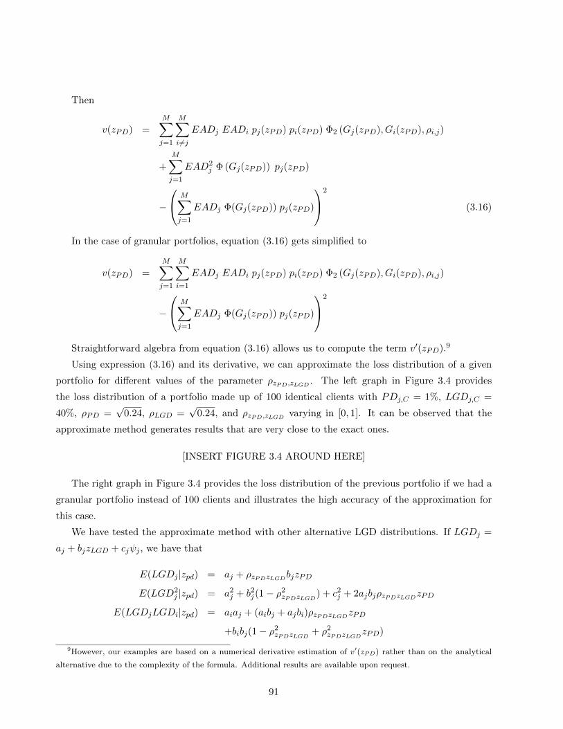
Then
v(zPD) =M∑j=1
M∑i 6=j
EADj EADi pj(zPD) pi(zPD) Φ2 (Gj(zPD), Gi(zPD), ρi,j)
+M∑j=1
EAD2j Φ (Gj(zPD)) pj(zPD)
−
M∑j=1
EADj Φ(Gj(zPD)) pj(zPD)
2
(3.16)
In the case of granular portfolios, equation (3.16) gets simplified to
v(zPD) =
M∑j=1
M∑i=1
EADj EADi pj(zPD) pi(zPD) Φ2 (Gj(zPD), Gi(zPD), ρi,j)
−
M∑j=1
EADj Φ(Gj(zPD)) pj(zPD)
2
Straightforward algebra from equation (3.16) allows us to compute the term v′(zPD).9
Using expression (3.16) and its derivative, we can approximate the loss distribution of a given
portfolio for different values of the parameter ρzPD,zLGD . The left graph in Figure 3.4 provides
the loss distribution of a portfolio made up of 100 identical clients with PDj,C = 1%, LGDj,C =
40%, ρPD =√
0.24, ρLGD =√
0.24, and ρzPD,zLGD varying in [0, 1]. It can be observed that the
approximate method generates results that are very close to the exact ones.
[INSERT FIGURE 3.4 AROUND HERE]
The right graph in Figure 3.4 provides the loss distribution of the previous portfolio if we had a
granular portfolio instead of 100 clients and illustrates the high accuracy of the approximation for
this case.
We have tested the approximate method with other alternative LGD distributions. If LGDj =
aj + bjzLGD + cjψj , we have that
E(LGDj |zpd) = aj + ρzPDzLGDbjzPD
E(LGD2j |zpd) = a2
j + b2j (1− ρ2zPDzLGD
) + c2j + 2ajbjρzPDzLGDzPD
E(LGDjLGDi|zpd) = aiaj + (aibj + ajbi)ρzPDzLGDzPD
+bibj(1− ρ2zPDzLGD
+ ρ2zPDzLGD
zPD)
9However, our examples are based on a numerical derivative estimation of v′(zPD) rather than on the analytical
alternative due to the complexity of the formula. Additional results are available upon request.
91

As before we set LGD∗j = E(LGDj |zpd), then we have
E(L|L) =M∑j=1
EADj E(LGDj |zpd) pj(zPD)
v(zPD) =
M∑j=1
M∑i 6=j
EADj EADi pj(zPD) pi(zPD) E(LGDjLGDi|zpd)
+M∑j=1
EAD2j E(LGD2
j |zpd) pj(zPD)
−
M∑j=1
EADj E(LGDj |zpd) pj(zPD)
2
In Figure 3.5 we show the result of the approximate method and the Monte Carlo method under
Gaussian recoveries.10 The correlation between the two macroeconomic factors varies between 0
and -1, where the value -1 implies the maximum positive correlation between default and loss given
default. It can be observed that the model accuracy is very high.
[INSERT FIGURE 3.5 AROUND HERE]
Finally, for LGDj = eaj+bjzLGD+cjψj , we get
E(
(LGDj)k∣∣∣ zpd) = ekµ1+ 1
2(kσ1)2
, k = 1, 2
with
µ1 = aj + ρzPDzLGDbjzPD
σ21 = b2j (1− ρ2
zPDzLGD) + c2
j
Moreover, we obtain
E(LGDjLGDi|zpd) = eµ2+ 12σ2
2
with
µ2 = (ai + aj) + (bi + bj)ρzPD,zLGDzPD
σ22 = c2
i + c2j + (1− ρ2
zPD,zLGD)(bi + bj)
2
Figure 3.6 shows the results for the lognormal recoveries11 and illustrates that the model perfor-
mance is very similar to that of Gaussian recoveries.
[INSERT FIGURE 3.6 AROUND HERE]
10We use PDj,C = 1%, ρPD =√
0.24, aj = 0.19, bj = 0.08, and cj = 0.11.11We use PDj,C = 1%, ρPD =
√0.24, aj = −1.88, bj = 0.4, and cj = 0.51.
92

3.6 Conclusions
This paper has described the Taylor expansion based method introduced in Pykhtin (2004) and
applied it to measure the credit risk of the Spanish financial system. We have shown that in the case
of concentrated portfolios the approximation does not perform very well and it can underestimate
the probability of high losses. We have also shown that the risk allocation based on this method
does not generate accurate results for our portfolio. This is the case for the VaR and the ES based
risk allocation. Additionally we have evaluated different ways to allocate the risk based on three
different derivation rules.
We have also introduced a simple model to consider the effect of correlated random recoveries
on the Basel capital requirements formula. The main drawback of this model is that it does not
allow for any diversification effect as it assumes that the defaults and the recoveries are driven by
the same macroeconomic factor.
Finally we have built a more flexible model that considers correlated random recoveries and we
have used the Taylor expansion method to approximate the loss distribution. Our results suggest that
this a robust method that generates accurate results and that can handle many different recoveries
distributions. We believe that this method can be easily implemented under the Basel capital charge
framework in order to consider the correlated random recoveries.
93

Appendix of Figures
0 1 2 3 4 5 6 7 8
x 104
10−6
10−5
10−4
10−3
10−2
10−1
100
Loss (MM )
Tai
l pro
babi
lity
Loss Distribution
MC 1,000,000Pykhtin 1Pykhtin 2
0 0.5 1 1.5 2 2.5 3 3.5 4 4.5 5
x 104
0
0.5
1
1.5
2
2.5
3
3.5
4
4.5
5x 10
4
Loss (MM )
ES
(M
M )
Expected Shortfall
MC 1,000,000Pykhtin 1Pykhtin 2
Figure 3.1: Loss distribution and expected shortfall for the Spanish financial institutions. These results are
obtained using a Monte Carlo method with 1,000,000 simulations (MC) and the Pykhtin approximation when
only the first term or both terms are considered (Pykhtin 1, Pykhtin 2). The black line indicates the MC
results and the blue crosses and the red circles are the Pykhtin 1 and Pykhtin 2 results, respectively. Left
and right graphs show the loss distribution and the expected shortfall results, respectively.
94

0
20
40
60
80
100
%
CVaR Loss (99.9%) Allocation
SANTANDER
BBVA
BANKIA
LA C
AIXA
POPULAR
SABADELL
CATALUNYACAIX
ANCG
BANCA CIV
ICACAM
MARE N
OST.
BANKINTER, S
ABASE
CAJA E
SPAÑABBK
IBERCAJA
UNICAJA
BARCLAYS
BANCO PASTOR
UNIMM
CAJAM
AR
BANCO DE V
ALENCIA
CAJA L
ABORAL
KUTXA
CAJA 3
Pykthin Num. Der.Pykthin Num. Der. Const.Pykthin Anal.MC 1,000,000
0
5
10
15
20
25
30
35
40
%
CES Loss (99.9%) Allocation
SANTANDER
BBVA
BANKIA
LA C
AIXA
POPULAR
SABADELL
CATALUNYACAIX
ANCG
BANCA CIV
ICACAM
MARE N
OST.
BANKINTER, S
ABASE
CAJA E
SPAÑABBK
IBERCAJA
UNICAJA
BARCLAYS
BANCO PASTOR
UNIMM
CAJAM
AR
BANCO DE V
ALENCIA
CAJA L
ABORAL
KUTXA
CAJA 3
Pykthin Num. Der.Pykthin Num. Der. Const.Pykthin Anal.MC 1,000,000
Figure 3.2: Risk allocation for the Spanish financial institutions. These results are obtained using a Monte
Carlo method with 1,000,000 simulations (MC) and the Pykhtin approximation derivatives, using a numerical
derivation method and the analytical derivation formula (Pykthin Anal.). We use two types of numerical
derivations, one that varies the values of aj and bf as λ varies on the derivation process (Pykthin Num. Der.)
and another one that maintains them constant (Pykthin Num. Der. Const.). Left and right graphs show the
loss allocation result based on the VaR and the expected shortfall criteria, respectively.
0 0.05 0.1 0.15 0.2 0.25 0.310
−4
10−3
10−2
10−1
Constant Vs Random LGD models comparison
Default Rate
1−C
umul
ativ
e P
roba
bilit
y
Const.00.10.20.30.40.50.60.70.80.91
0 0.1 0.2 0.3 0.4 0.5 0.6 0.7 0.8 0.9 11
1.5
2
2.5LGD Adjustment (99.9%)
Rho LGD
x LG
D A
djus
tem
ent
Figure 3.3: Simplified random LGD model. The left graph shows the tail loss for the cases of constant LGD
(Const.) and for ρLGD varying in [0, 1]. The right graph provides the constant LGD multiplier required to
achieve the random LGD 99.9% probability loss as the parameter ρLGD increases.
95
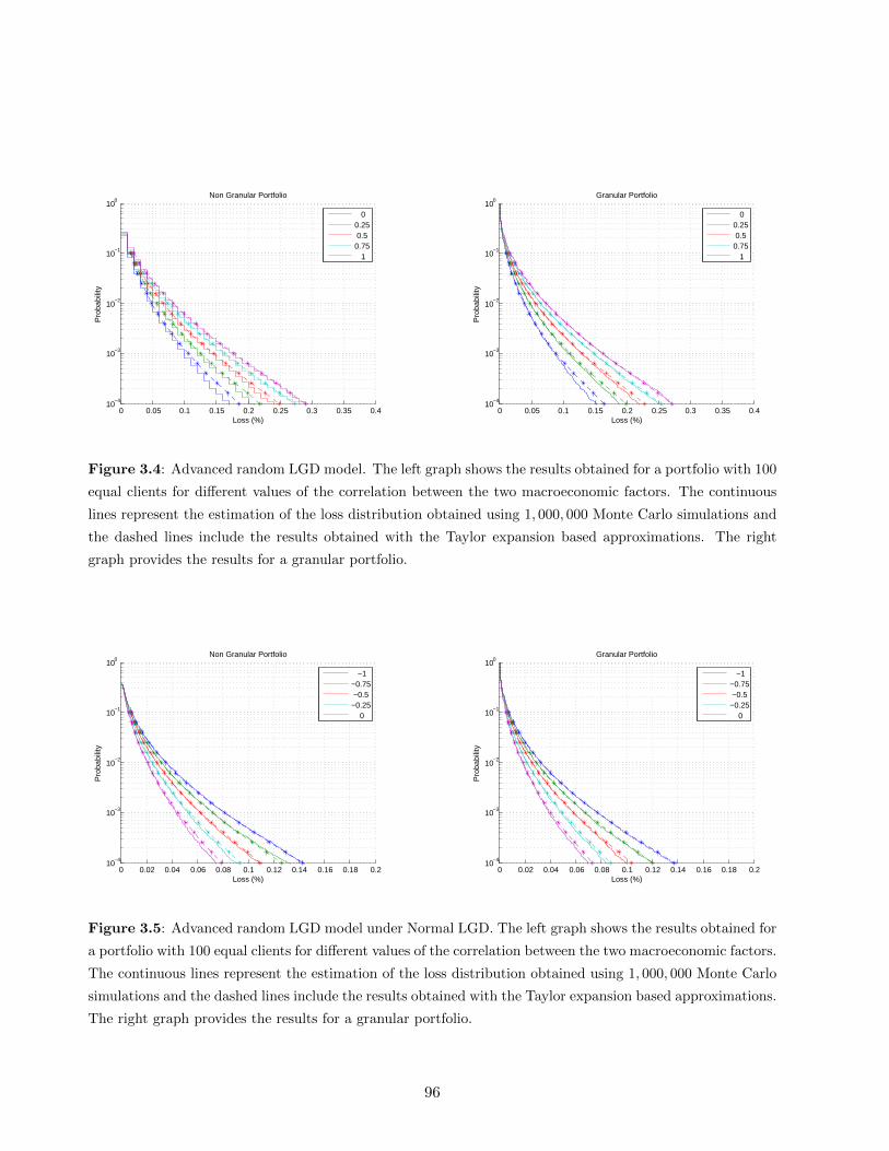
0 0.05 0.1 0.15 0.2 0.25 0.3 0.35 0.410
−4
10−3
10−2
10−1
100
Non Granular Portfolio
Loss (%)
Pro
babi
lity
00.25 0.50.75 1
0 0.05 0.1 0.15 0.2 0.25 0.3 0.35 0.410
−4
10−3
10−2
10−1
100
Granular Portfolio
Loss (%)
Pro
babi
lity
00.25 0.50.75 1
Figure 3.4: Advanced random LGD model. The left graph shows the results obtained for a portfolio with 100
equal clients for different values of the correlation between the two macroeconomic factors. The continuous
lines represent the estimation of the loss distribution obtained using 1, 000, 000 Monte Carlo simulations and
the dashed lines include the results obtained with the Taylor expansion based approximations. The right
graph provides the results for a granular portfolio.
0 0.02 0.04 0.06 0.08 0.1 0.12 0.14 0.16 0.18 0.210
−4
10−3
10−2
10−1
100
Non Granular Portfolio
Loss (%)
Pro
babi
lity
−1−0.75 −0.5−0.25 0
0 0.02 0.04 0.06 0.08 0.1 0.12 0.14 0.16 0.18 0.210
−4
10−3
10−2
10−1
100
Granular Portfolio
Loss (%)
Pro
babi
lity
−1−0.75 −0.5−0.25 0
Figure 3.5: Advanced random LGD model under Normal LGD. The left graph shows the results obtained for
a portfolio with 100 equal clients for different values of the correlation between the two macroeconomic factors.
The continuous lines represent the estimation of the loss distribution obtained using 1, 000, 000 Monte Carlo
simulations and the dashed lines include the results obtained with the Taylor expansion based approximations.
The right graph provides the results for a granular portfolio.
96

0 0.02 0.04 0.06 0.08 0.1 0.12 0.14 0.16 0.18 0.210
−4
10−3
10−2
10−1
100
Non Granular Portfolio
Loss (%)
Pro
babi
lity
−1−0.75 −0.5−0.25 0
0 0.02 0.04 0.06 0.08 0.1 0.12 0.14 0.16 0.18 0.210
−4
10−3
10−2
10−1
100
Granular Portfolio
Loss (%)
Pro
babi
lity
−1−0.75 −0.5−0.25 0
Figure 3.6: Advanced random LGD model under Lognormal LGD. The left graph shows the results obtained
for a portfolio with 100 equal clients for different values of the correlation between the two macroeconomic
factors. The continuous lines represent the estimation of the loss distribution obtained using 1, 000, 000
Monte Carlo simulations and the dashed lines include the results obtained with the Taylor expansion based
approximations. The right graph provides the results for a granular portfolio.
97

Conclusions
The credit risk model proposed in Vasicek (1987) is the most common method to measure credit
risk. However, under this model, estimating the loss distribution of a given portfolio usually requires
Monte Carlo simulations. Estimating and allocating the credit risk of a portfolio using this type of
simulations can be a very time demanding procedure. As a consequence alternative techniques have
arisen to optimize the risk measurement process. This thesis has provided several contributions to
the literature on credit risk from both methodological and empirical points of view.
From a methodological point of view, we have studied and extended the methods to estimate
the credit risk of a portfolio presented in Pykhtin (2004), Glasserman and Li (2005), and Huang
et al. (2007). We have modified the importance sampling and saddlepoint methods to work under
random recoveries and market valuation. Additionally in the case of the saddlepoint method we
have proposed a new risk allocation method that uses the Hermite polynomials. This new method
has performed better than other approximate methods currently available (see Martin and Thomp-
son (2001)) and, compared with an exact method, it has produced similar results but with fewer
calculations.
Using the Taylor expansion based approximate methods we have developed a random LGD model
that has allowed to consider the correlation between the default and the recoveries. Compared with
a Monte Carlo method the results of this approximate method are very similar but this method has
the advantage of providing a closed-form representation. Other methodological contributions that
can be found in this thesis are the “multimodal distributions” and “loop decoupling” that allowed for
a faster and more accurate estimation of the credit risk under the importance sampling method.
From an empirical point of view, we have obtained the loss distribution of the Spanish financial
system based on the models and extensions previously mentioned. Additionally we have allocated
the risk over the financial institutions in the financial system. We have used the data of the Spanish
financial system at December 2010 and obtained the loss distribution under constant LGD for the
three credit risk models analyzed. Compared with Campos et al. (2007) we have provided the
detailed steps used to calibrate all the model parameters, even the LGD, and allowed institutions to
be exposed to more than one macroeconomic factor.
98

We have also quantified the variability of the loss distribution by means of two different analysis:
i) first, we have obtained the loss distribution at December 2007, a pre-crisis year and ii) secondly,
we have studied the uncertainty in the model parameters, αf,j , PD, and LGD. This uncertainty
comes from the lack of long enough historical time series to calibrate these parameters. The main
qualitative conclusion of this analysis is that the LGD is the main source of uncertainty in the loss
distribution estimation.
Under constant LGD the importance sampling and the saddlepoint methods have provided very
accurate results; however the Taylor expansion based method introduced in Pykhtin (2004) has not
been able to capture accurately the concentration profile of our portfolio. The same has happened
for the risk allocation.
For the importance sampling and saddlepoint methods we have also obtained the loss distribution
of the portfolio under random LGD and market valuation. We have provided all the detailed steps
to calibrate the model parameters. Under random LGD the loss distribution is slightly shifted to the
right compared with the constant LGD case and the results for the different random LGD models
have been very similar, even between the pure macroeconomic models and the mixed idiosyncratic
and macroeconomic models. When we have moved to the market valuation, the loss distribution
gets considerably shifted to the right as we have more states that produce high losses.
Regarding the risk allocation we have shown that the risk allocated is very sensitive to the
allocation criteria and to the loss definition. In the extreme, under constant LGD and VaR based
risk allocation, Santander and BBVA have been allocated a null risk. In the case of the Hermite
polynomials based risk allocation new method that we have proposed, the results for the portfolio
have been very satisfactory. The method has shown to be more accurate than other approximate
methods (see Martin and Thompson (2001)) while requiring a similar number of calculations.
Given our results for the portfolio we suggest not to focus on a unique model or risk allocation
criteria but to test several of them. We consider that this thesis has contributed to the previous
literature with new methodological issues and empirical results related to the measurement of credit
risk. The methods we have proposed can be used directly by practitioners and regulators to monitor
the credit risk of given portfolios. Finally, in the case of regulators some of the ideas proposed and
developed in this thesis can serve as a reference to identify and monitor the so called systemically
important financial institutions (SIFIs).
99

Conclusiones
El modelo de riesgo de credito propuesto en Vasicek (1987) es el metodo mas habitual para medir
el riesgo de credito. Sin embargo, estimar la distribucion de perdidas de una cartera bajo este
modelo suele requerir la utilizacion de simulaciones Monte Carlo. La estimacion y reparto del riesgo
de credito de una cartera empleando este tipo de metodo de simulacion puede ser un proceso que
requiera un elevado consumo de tiempo. Como consecuencia han surgido tecnicas alternativas para
optimizar el proceso de medicion del riesgo. Esta tesis proporciona diversas contribuciones a la
literatura del riesgo de credito tanto desde un punto de vista metodologico como empırico.
Desde un punto de vista metodologico, hemos estudiado y extendido los metodos para cuantificar
el riesgo de credito de una cartera presentados en Pykhtin (2004), Glasserman and Li (2005) y Huang
et al. (2007). Hemos modificado los metodos de muestreo por importancia y de saddlepoint para
los casos de recuperaciones aleatorias y valoracion de mercado. Adicionalmente, en el caso de
los metodos de saddlepoint, hemos propuesto un nuevo metodo para repartir el riesgo que emplea
polinomios de Hermite. Este nuevo metodo se comporta mejor que otros metodos aproximados
disponibles actualmente (ver Martin and Thompson (2001)) y, comparado con un metodo exacto,
produce resultados similares pero con un numero menor de calculos.
Empleando los metodos aproximados basados en expansiones de Taylor hemos desarrollado un
modelo de LGD aleatoria que nos permite considerar la correlacion entre el incumplimiento y las
recuperaciones. Comparado con el metodo Monte Carlo los resultados de este metodo aproximado
son muy similares pero este metodo tiene la ventaja de proporcionar una representacion analıtica.
Otras contribuciones metodologicas que se encuentran en esta tesis son las llamadas “distribuciones
multimodales” y el “desacople de bucles” que permiten una estimacion del riesgo de credito mas
rapida y precisa cuando se utiliza el metodo del muestreo por importancia.
Desde un punto de vista empırico, hemos obtenido la distribucion de perdidas del sistema fi-
nanciero espanol empleando los modelos y extensiones mencionadas previamente. Adicionalmente
hemos repartido el riesgo entre las distintas instituciones financieras. Hemos empleado datos del sis-
tema financiero espanol correspondientes a Diciembre de 2010 y obtenido la distribucion de perdidas
bajo LGD constante para los tres modelos de riesgo de credito analizados. Comparado con Cam-
100

pos et al. (2007) presentamos los pasos detallados seguidos para calibrar todos los parametros del
modelo, incluida la LGD, y permitimos que las instituciones financieras esten expuestas a mas de
un factor macroeconomico.
Tambien hemos cuantificado la variabilidad de la distribucion de perdidas realizando dos tipos
de analisis: i) primero, hemos obtenido la distribucion de perdidas en Diciembre de 2007, una fecha
anterior a la crisis y ii) segundo, hemos estudiado la incertidumbre en los parametros αf,j , PD y
LGD del modelo. Esta incertidumbre proviene de la ausencia de series temporales suficientemente
largas para calibrar estos parametros. La principal conclusion cualitativa de este analisis es que la
LGD es la principal fuente de incertidumbre en la estimacion de la distribucion de perdidas.
Considerando LGD constante, los metodos de muestreo por importancia y de saddlepoint han
proporcionado resultados muy precisos; sin embargo el metodo basado en la expansion de Taylor
propuesto en Pykhtin (2004) no ha sido capaz de capturar adecuadamente el perfil de concentracion
de nuestra cartera. La misma conclusion se obtiene para el reparto del riesgo.
Adicionalmente, para los metodos de muestreo por importancia y de saddlepoint, hemos obtenido
la distribucion de perdidas de la cartera considerando LGD aleatoria y valoracion de mercado.
Hemos proporcionado todos los pasos detallados para calibrar los parametros del modelo. Bajo
LGD aleatoria la distribucion de perdidas se desplaza ligeramente a la derecha comparada con el
caso de LGD constante y los resultados para los distintos modelos de LGD aleatoria han sido simi-
lares, incluso entre los modelos de recuperaciones macroeconomicas y los modelos de recuperaciones
macroeconomicas e idiosincraticas. Cuando consideramos la valoracion de mercado, la distribucion
de perdidas se desplaza considerablemente a la derecha pues, en este caso. tenemos mas estados que
producen perdidas elevadas.
Hemos mostrado que el reparto del riesgo es muy sensible al criterio de reparto y a la definicion
de perdidas empleada. En el caso extremo de LGD constante y reparto de riesgo basado en el VaR,
se asigna un riesgo nulo a Santander y BBVA. En el caso del nuevo metodo de reparto basado en
polinomios de Hermite, los resultados para la cartera han sido muy satisfactorios. El metodo ha
generado una mayor precision que otros metodos aproximados (ver Martin and Thompson (2001))
mientras que requiere un numero similar de calculos.
De acuerdo a nuestros resultados empıricos sugerimos contrastar varios modelos o criterios de
reparto. Consideramos que esta tesis ha contribuido a la literatura previa sobre la medicion del riesgo
de credito con nuevas propuestas metodologicas y resultados empıricos novedosos y utiles a nivel
practico. Los metodos que hemos propuesto pueden ser empleados directamente por reguladores y la
industria bancaria para monitorizar las carteras. Finalmente, en el caso de los reguladores, algunas
de las ideas propuestas y desarrolladas en esta tesis pueden servir como referencia para identificar y
monitorizar las conocidas como instituciones financieras sistemicamente importantes (SIFIs).
101
References
Abate, J. and Whitt, W. (1995). Numerical inversion of Laplace transforms. ORSA Journal on
Computing, 7 (1), 36-43.
Abramowitz, M. and Stegun, I.A. (1964). Handbook of mathematical functions with formulas, graphs
and mathematical tables, Courier Dover Publications.
Allen, F., Bartiloro, L. and Kowalewski, O. (2006). The Financial System of the EU 25, In Finan-
cial Development, Integration and Stability: Evidence from Central, Eastern and South-Eastern
Europe, edited by K. Liebscher, J. Christl, P. Mooslechner and D. Ritzberger-Grunwald, Edward
Elgar, Cheltenham.
Altman, E.I., Brady, B., Resti, A. and Sironi, A. (2005). The link between default and recovery
rates: Theory, empirical evidence and implications. Journal of Business, 78 (6), 2203-2227.
Altman, E.I. and Kishore, V.M. (1996). Almost Everything You Wanted to Know about Recoveries
on Defaulted Bonds. Financial Analysts Journal, 52 (6), 57-64.
Altman, E.I and Suggitt, H. (2000). Default rates in the syndicated bank loan market: A mortality
analysis. Journal of Banking and Finance, 24 (1-2), 229-253.
Amihud, Y., Garbade, K. and Kahan, M. (2000). An institutional innovation to reduce agency costs
of public corporate bonds. Journal of Applied Corporate Finance, 13 (1), 114-121.
Basel Committee on Bank Supervision (2006). Basel II: International Convergence of Capital Mea-
surement and Capital Standards: A Revised Framework - Comprehensive Version. Available at
http://www.bis.org.
Basel Committee on Bank Supervision (2011). Global systemically important banks: Assessment
methodology and the additional loss absorbency requirement. Available at http://www.bis.org.
BBVA Bank (2009). 2008 Annual Report. Available at http://www.bbva.com.
102

Bennet, R.L. (2002). Evaluating the adequacy of the deposits insurance fund: A Credit-Risk mod-
eling approach. FDIC Working Papers, No. 2001-2002.
Bennet, R.L. and Unal, H. (2011). The cost effectiveness of the private sector reorganization of failed
banks. FDIC Working Papers, No. 2009-2011.
Campos, P., Yague, M. and Chinchetru, I. (2007). Un nuevo marco de seguro de depositos para
Espana. Banco de Espana Estabilidad Financiera, 12, 93-110.
Cantor, R., Hamilton, D. and Tennant, J. (2007). Confidence Intervals for Corporate Default Rates.
Moody’s Special Comment, Moody’s Investors Service.
Carbo, S., Humphrey, D., Maudos, J. and Molyneux, P. (2009). Cross-country comparisons of com-
petition and pricing power in European banking. Journal of International Money and Finance,
28 (1), 115-134.
Carey, M. (1998). Credit risk in private debt portfolios. Journal of Finance, 53 (4), 1363-1387.
Cariboni, J., Maccaferri, S. and Schoutens, W. (2011). Applying Credit Risk Techniques to Design an
Effective Deposit Guarantee Schemes Funds. International Risk Management Conference working
Paper.
Castro, C. (2012). Confidence sets for asset correlations in portfolio credit risk. Revista de Economia
del Rosario, 15 (1), 19-58.
Chance, D. M. and Agca, S. (2003). Speed and Accuracy Comparisons of Bivariate Normal Prob-
ability Distribution Approximations for Option Pricing. Journal of Computational Finance, 6,
61-96.
Daniels, H.E. (1954). Saddlepoint approximations in statistics. The Annals of Mathematical Statis-
tics, 25 (4), 631-650.
Daniels, H.E. (1980). Exact saddlepoint approximations. Biometrika, 67 (1), 59-63.
Daniels, H.E. (1987). Tail probability approximations. International Statistical Review, 55 (1), 37-48.
Dullmann, K., Kull, J. and Kunisch M. (2008). Estimating asset correlations from stock prices or
default rates which method is superior?. Deutsche Bundesbank Banking and Financial Studies, No
04/2008.
Fitch (2009). Global Corporate Finance 2008 Transition and Default Study. Credit Market Research,
Fitch Corporation.
103
Garcıa-Cespedes, R. and Moreno, M. (2014). Estimating the distribution of total default losses on
the Spanish Financial system, mimeo, BBVA and University of Castilla-La Mancha.
Garcıa-Cespedes, R. and Moreno, M. (2014b). Extended saddlepoint methods for credit risk mea-
surement, mimeo, BBVA and University of Castilla-La Mancha.
Genz, A. (2004). Numerical Computation of Rectangular Bivariate and Trivariate Normal and t
Probabilities. Statistics and Computing, 14, 151-160.
Glasserman, P. (2005). Measuring Marginal Risk Contributions in Credit Portfolios. Journal of
Computational Finance, 9 (2), 1-41.
Glasserman, P. and Li, J. (2005). Importance Sampling for Portfolio Credit Risk. Management
Science, 51 (11), 1643-1653.
Glasserman, P. and Ruız-Mata, J. (2006). Computing the credit loss distribution in the Gaussian
copula model: a comparison of methods. Journal of Credit Risk, 2 (4), 33-66.
Gordy, M. (2000). A comparative anatomy of credit risk models. Journal of Banking and Finance,
24, 119-149.
Gourieroux, C., Laurent, J.P. and Scaillet, O. (2000). Sensitivity Analysis of Values at Risk. Journal
of Empirical Finance, 7 (3-4), 225-245.
Grundke, P. (2009). Importance sampling for integrated market and credit portfolio models. Euro-
pean Journal of Operational Research, 194 (1), 206-226.
Gupton, G.M. and Stein, R.M. (2002). LossCalcTM : Moody’s model for predicting loss given default
(LGD). Moody’s Investor Service, February.
Hanson, S.G. and Schuermann, T. (2006). Confidence intervals for probabilities of default. Journal
of Banking and Finance, 30 (8), 2281-2301.
Hartmann, P., Ferrando, A., Fritzer, F., Heider, F., Lauro, B. and Lo Duca, M. (2006). The Perfor-
mance of the European Financial System, mimeo, European Central Bank, August.
Huang, X., Oosterlee, C.W. and Van Der Weide, H. (2007). Higher Order Saddlepoint Approx-
imations on the Vasiceck Portfolio Credit Loss Model. Journal of Computational Finance, 11,
93-113.
Hull, J. (2011). Options, Futures, and Other Derivatives, eighth edn. Prentice Hall.
James, C. (1991). The loss realized in banks failures. Journal of Finance, 46, 1223-1242.
104

Kaufman, G. (2004). FDIC Losses in Bank Failures: Has FDICIA made a difference?. Federal Reserve
Bank of Chicago working paper.
Kuritzkes, A., Schuermann, T. and Weiner, S. (2002). Deposit Insurance and Risk Management
of the U.S. Banking System: How Much? How Safe? Who Pays?. Wharton School Center for
Financial Institutions Working Papers, 02-02.
Lee, J., Wang, J. and Zhang, J. (2009). The relationship between average asset correlation and
default probability. Moody’s KMV Company.
Lopez, J. (2002). The Empirical Relationship between Average Asset Correlation, Firm Probability
of Default and Asset Size. Federal Reserve Bank of San Francisco.
Martin, R. and Thompson, K. (2001). VaR: who contributes and how much?. Risk Magazine, 14 (8),
99-103.
Martin, R. and Wilde, T. (2002). Unsystematic Credit Risk. Risk Magazine, 15 (11), 123-128.
Moody’s (2005). Default, Losses and Rating Transitions on Bonds Issued by Financial Institutions:
1983-2004. Moody’s Investor service.
Moody’s (2009). Corporate Default and Recovery rates 1920-2008. Moody’s Investor service.
Morone, M., Cornaglia, A. and Mignola, G. (2012) Determining marginal contributions of the eco-
nomic capital of credit risk portfolio: an analytical approach, mimeo, Intesa Sanpaolo.
Owen, D. B. (1956). Tables for computing bi-variate normal probabilities. Annals of Mathematical
Statistics, 27(4), 1075-1090.
Pykhtin, M. (2004). Multi-factor adjustment. Risk Magazine, 17 (3), 85-90.
Qibin, C., Amnon, L. and Nihil, P. (2009). Understanding asset correlation dynamics from stress
testing. Moody’s KMV Company.
Reid, N. (1988). Saddlepoint methods and statistical inference. Statistical Science, 3 (2), 213-238.
Reitan, T. and Aas, K. (2010). A new robust importance-sampling method for measuring value-at-
risk and expected shortfall allocations for credit portfolios. Journal of Credit Risk, 6 (4), 113-149.
Repullo, R., Saurina, J. and Trucharte, C., 2010. Mitigating the pro-cyclicality of Basel II. Economic
Policy, 25 (64), 659-702.
Santander Bank (2009). 2008 Annual Report. Available at http://www.santander.com.
105

Schuermann, T. (2004). What do we know about loss given default? In: Shimko, D. (Ed.), Credit
Risk: Models and Management, second ed. Risk Books, London, UK (chapter 9).
Serfling, R.J. (1980). Approximation Theorems of Mathematical Statistics. John Wiley & Sons.
S&P (2009). 2008 Annual Global Corporate Default Study And Rating Transitions. S&P Corporation
Ratings Direct.
S&P (2010). 2009 Annual Global Corporate Default Study And Rating Transitions. S&P Corporation
Ratings Direct.
Thorburn, K. (2000). Bankruptcy auctions: costs, debt recovery and firm survival. Journal of Fi-
nancial Economics, 58 (3), 337-368.
Tsao, M. (1995). Asymptotic and numerical methods for approximating distributions. PhD Thesis,
Simon Fraser University.
Unal, H., Madan, D. and Guntay, L. (2003). Pricing the risk of recovery in default with APR
violations. Journal of Banking and Finance, 27 (6), 1001-1025.
Vasicek, O.A. (1987). Probability of loss on loan portfolio. Working Paper, KMV Corporation.
Vasicek, O.A. (1996). A Series Expansion for the Bivariate Normal Integral. Working Paper, KMV
Corporation.
Voropaev, M. (2011). An analytical framework for credit portfolio risk measures. Risk Magazine, 24
(5), 72-78.
106
Related Documents