TESI On the Proof of E¢ cacy of Functional Foods: Design Considerations · UNIVERSITA™DEGLI STUDI DI MILANO BICOCCA DOTTORATO DI RICERCA IN STATISTICA XXIII CICLO TESI On the Proof

UNIVERSITA’DEGLI STUDI DI MILANO BICOCCA

DOTTORATO DI RICERCA IN STATISTICA

XXIII CICLO

TESI

On the Proof of Effi cacy of Functional Foods:Design Considerations

Relatore:

Prof. Dario Gregori

Candidata:

Dott.ssa Ileana Baldi

2011

Contents

1 Introduction 1

2 Functional Foods 32.1 Regulation and health claims for functional foods . . . . . . . 4

2.2 Endpoint identification . . . . . . . . . . . . . . . . . . . . . . 8

2.3 Study design . . . . . . . . . . . . . . . . . . . . . . . . . . . . 10

3 Surrogate Endpoints 113.1 Validation on individual data . . . . . . . . . . . . . . . . . . 12

3.2 Validation on summary statistics: a meta-analysis perspective 18

4 Evidence-based research 224.1 Evidence-based nutrition . . . . . . . . . . . . . . . . . . . . . 25

4.2 Continuos data . . . . . . . . . . . . . . . . . . . . . . . . . . 25

4.3 Validation of a prognostic model . . . . . . . . . . . . . . . . . 28

5 Surrogate Endpoint for Cardiovascular Risk Reduction: acase-study 305.1 Methods . . . . . . . . . . . . . . . . . . . . . . . . . . . . . . 31

5.2 Results . . . . . . . . . . . . . . . . . . . . . . . . . . . . . . . 34

5.3 Discussion . . . . . . . . . . . . . . . . . . . . . . . . . . . . . 40

6 Conclusions 41

7 Appendix 43

References 59

1

1 Introduction

At the turn of the 21st century, modern society faces new challenges, from

exponentially growing costs of health care, increase in life expectancy, im-

proved scientific knowledge, and development of new technologies to major

changes in lifestyles. Nutrition has to adapt to these new challenges by devel-

oping new concepts. Optimal nutrition is one of these, aimed at maximizing

physiologic functions of each individual to ensure both maximum well-being

and health, and, at the same time, confer a minimum risk of disease through-

out the lifespan. Although the connection between diet and health has long

been recognized, currently we are learning more about how global lifestyle

and dietary approaches can prevent disease. Knowledge of the role of phys-

iologically active food components, from plant, animal, and microbial food

sources, has changed the role of diet in health. Nutritional issues have shown

the relationship between diet and ageing, obesity, heart disease, and cancer

[1].

Many interventions have been proposed through policy makers, most of

them regarding the deprivation of normal components (salt, sugar or fat) in

order to provide healthier products. A different proposal has, as principal

category of interest, functional food, with the aim of following usual dietary

pattern, adding functionality to the common nutrients.

By definition, functional foods benefit human health beyond the effect of

nutrients alone. Functional foods have evolved as food and nutrition science

has advanced beyond the treatment of deficiency syndromes to reduction of

disease risk and health promotion and, owing to their ability to confer health

and physiological benefits, are increasing in popularity.

The aims of functional food science, as summarized in [2], are, to iden-

tify beneficial interactions between a functional food component and one or

more target functions in the body and to obtain evidence for the underlying

mechanisms; to identify and validate markers for these functions and their

modulation by food components; to assess the safety of the amount of food

1

or its components needed for functionality; to formulate hypotheses to be

tested in human intervention studies that aim to show that the relevant in-

take of specified food components is associated with improvement in one or

more target functions, either directly, or in terms of a valid marker of an

improved state of health and well-being and/or a reduced risk of a disease.

A sound scientific evidence from such studies, both observational studies and

randomized clinical trials (RCTs), is required to substantiate claims on a

functional food.

A direct measurement of the effect a food on health and well-being and/or

reduction of disease risk is often not possible. Therefore, one key, but diffi cult,

step in the development of functional foods is the identification and validation

of relevant markers that can predict potential benefits or risks relating to

certain health conditions.

The second key step, once the surrogate has been identified and validated,

is to frame the proof within a study design that is able to link the inference

on the surrogate with the inference that would be made on the true endpoint,

had it been observed.

The aim of this work is to address this research question, by assuming that

there is a known relationship between the surrogate and the true endpoint

explored during the surrogacy assessment. Statistical inference on the true

(unobserved) endpoint is derived on the basis of its predicted values.

After a brief review of the concept of statistical surrogacy, we illustrate

this approach through a motivating example from literature on surrogates

for cardiovascular risk prevention, integrated with simulated scenarios.

2

2 Functional Foods

The term “functional food”was introduced for the first time in the middle

of 1980s in Japan when, faced with escalating health care costs, the Ministry

of Health and Welfare initiated a regulatory system to approve certain foods

with documented health benefits in hopes of improving the health of the

nation’s aging population.

Several definitions of functional food exist. These include, the working

definition given by The European Commission Concerted Action on Func-

tional Food Science in Europe, co-ordinated by The International Life Sci-

ences Institute (ILSI- Europe) [2] that regards a food as functional “ if it is

satisfactorily demonstrated to affect beneficially one or more target functions

in the body, beyond adequate nutritional effects, in a way that is relevant to

either an improved state of health and well-being and/or reduction of risk of

disease”.

Functional foods may be broadly grouped into three categories: conven-

tional food containing naturally occurring bioactive substance, food to which

a component has been added or from which a component has been removed

by technological or biotechnological means, and food in which a component

has been modified in nature and/or bioavailability. Examples of these are

shown in Table 1.

Functional foods are not medicines. In fact, their purpose is to restore

or enhance normal function in order to optimize health, well-being and per-

formance, and to reduce risk factors for disease and not to treat or prevent

diseases, or to heighten physiological performance outside the normal range.

Functional foods are intended to be consumed as part of a normal diet and

they take the form of foods whereas medicines are intended to be taken as

part of a controlled regimen in tablets or pills which can be administered

in precise doses. Ultimately, the manufacture and marketing of medicines is

subject to different regulatory controls than those that apply to the manu-

facture and marketing of foods.

3

Functional food Food Component Potential health benefit

Spinach Calcium may reduce the risk of osteo-

porosis

Processed tomato prod-

ucts

Lycopene may contribute to maintenance

of prostate health

Table spreads (butter or

margarine alternatives)

fortified with stanol

and/or sterol esters

Stanol/Sterol

esters

may reduce the risk of coronary

heart disease (CHD)

Soy-based products Soy protein may reduce the risk of coronary

heart disease (CHD)

Wheat bran Insoluble Fiber may contribute to maintenance

of a healthy digestive tract may

reduce the risk of some types of

cancer

Table 1. Functional Foods Component Chart 2009. Adapted from International

Food Information Council (IFIC) Foundation

(http://www.ific.org/nutrition/functional/index.cfm).

2.1 Regulation and health claims for functional foods

Several mid- and long-term developments in society, as well as socio-demo-

graphic trends are in favor of functional food, so that it can be assumed

that functional food represents a sustainable category in the food market.

Moreover, it is beyond doubt that persuading people to make healthier food

choices would provide substantial (public) health effects, therefore it is a

common economic and public interest.

Foods are typically chosen for their good taste, convenience and price with

health being only one reason among many and functional foods are not ex-

ceptions in this. Consumers can only be expected to substitute conventional

4

with functional foods if these latter are perceived as comparatively healthy

and the promised health benefits are regarded as relevant. As consumers

become more health conscious, the demand and market value for health-

promoting foods and food components is expected to grow. Before the full

market potential can be realized, however, consumers need to be assured of

the safety and effi cacy of functional foods. These are two key aspects in a

potential food evaluation.

As in most other regulations, with Japan and its “foods for specified

health use, FOSHU”as a notable exception, in the USA and in Europe there

is no regulatory policy specific to functional foods. Rather they are regulated

under the same framework as conventional food.

As the relationship between nutrition and health gains public acceptance

and as the market for functional foods grows, the question of how to com-

municate the specific advantages of such foods becomes increasingly impor-

tant. The fundamental principle defining food allegations or claims is that

they must be scientifically proved, not ambiguous and clear to the consumer.

However, different definitions exist, depending on the country and its pol-

icy. In Europe, the Regulation 1924/2006/EC on nutrition and health claims

was agreed in December 2006 and came into force in 2007 [3]. The Regu-

lation 1924/2006/EC provides the definitions of nutrition claim (any claim

that states, suggests or implies that a food has particular beneficial nutri-

tional properties), health claim (any claim that states, suggests or implies

that a relationship exists between a food category, a food or one of its con-

stituents and health) and reduction of disease risk claim (any health claim

that states, suggests or implies that the consumption of a food category, a

food or one of its constituents significantly reduces the risk of a human dis-

ease) [4]. Health claims are divided into Article 14 and Article 13 claims

depending on whether they refer or not to either the reduction of disease risk

or to children’s development and health, respectively.

The assessment of the scientific evidence to support health claims is the

responsibility of the European Food Safety Authority (EFSA). In USA the

responsibility for ensuring the validity of these claims rests with the manufac-

turer, Food and Drug Administration (FDA), or, in the case of advertising,

5

with the Federal Trade Commission. Claims that can be used on food and

dietary supplement labels fall into three categories: health claims (imply a

relationship between dietary components and reducing risk of a disease or

health condition), nutrient content claims (characterize the level of a nutri-

ent or a dietary substance in a food), and structure/function claims (describe

the role of substances that affect normal functioning of the body).

The ways by which FDA exercises its oversight in determining which

health claims may be used on a label or in labeling for a food or dietary sup-

plement are the 1990 Nutrition Labeling and Education Act, the 1997 Food

and Drug Administration Modernization Act and the 2003 FDA Consumer

Health Information for Better Nutrition Initiative.

There are generally two types of labeling claims that embrace but are not

restricted to functional foods: structure/function claims (similar to Article 13

health claims in Europe) and health claims (similar to disease-risk reduction

claims in Europe). No statements about treating a disease should be made,

otherwise a functional food would be a drug [5].

Examples of strong scientific evidence of clinical effi cacy is for functional

foods that satisfied rich in fiber (oat brain or psyllium), which are associated

with several health effects. The major direct effects include improved bowel

function as treatment of irritable bowel syndrome, increased mineral absorp-

tion, altered lipid metabolism as reduced incidence of coronary heart disease

[1]. Examples of approved health claims by FDA are given in Table 2.

Several guidelines have been developed, for example, those in the USA,

Canada, Australia/New Zealand and the UK give detailed guidance on the

nature of scientific evidence required and suggest how it should be evaluated.

In Europe, the project “Process for the Assessment of Scientific Support for

Claims on Foods”(PASSCLAIM) had as its main objective the production

of a generic tool to assess the scientific support for health-related claims for

foods and food components [6]. The future of functional foods will undoubt-

edly involve a continuation of the labeling and safety debates.

6

Approved Health Claims Requirement for the food Model claim

Soluble Fiber (SF)

from certain foods

and risk of CHD

Low saturated fat

Low cholesterol

Low fat

Whole oat or barley foods*

>0.75 g SF/RACC

Oatrim

>0.75 g β-glucan SF/RACC

Psyllium husk

>1.7 g SF/RACC

The amount of SF/RACC

must be declared in

nutrition label.

SF from foods such as

[name of SF source, and,

if desired, name of food

product], as part of a diet

low in saturated fat and

cholesterol, may reduce

the risk of heart disease.

A serving of [name of

food product] supplies

. g of the [necessary

daily dietary intake

for the benefit] SF

from [name of SF source]

necessary per day

to have this effect.

Soy-protein

and risk of CHD

Low saturated fat

Low cholesterol

Low fat**

≥6.25 g soy protein/RACC

25 g of soy protein a day,

as part of a diet low in

saturated fat and

cholesterol, may

reduce the risk of heart

disease. A serving of

[name of food] supplies

. g of soy protein.

Table 2. Some approved health claim by FDA (CHD: Coronary Heart Disease;

RACC: Reference Amount Customarily Consumed; *include oat bran and/or rolled

oats and/or whole oat flour and/or whole grain barley or dry milled barley; **ex-

cept that foods made from whole soybeans that contain no fat in addition).

Adapted from: http://www.fda.gov/Food/GuidanceComplianceRegulatoryInfor-

mation/GuidanceDocuments/FoodLabelingNutrition/FoodLabelingGuide/

ucm064919.htm.

7

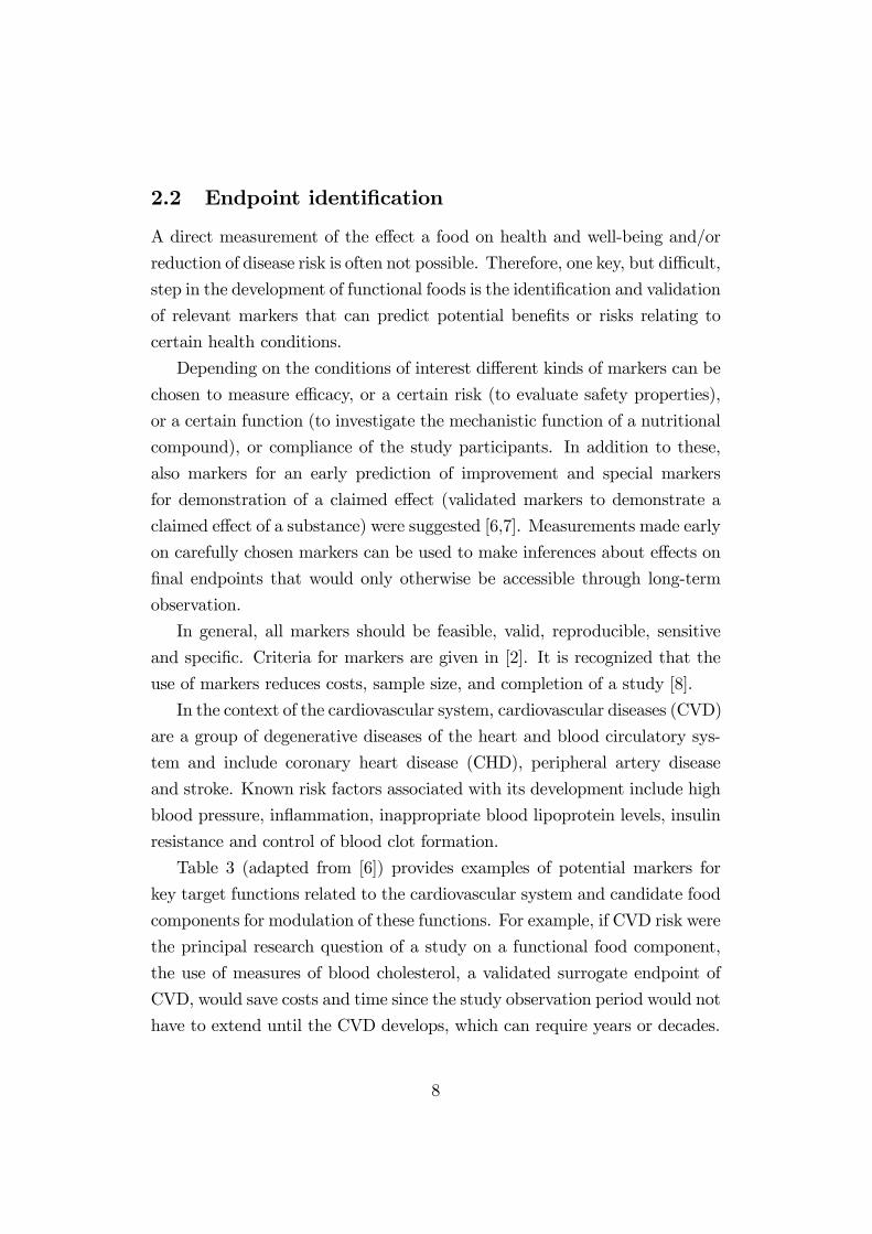
2.2 Endpoint identification

A direct measurement of the effect a food on health and well-being and/or

reduction of disease risk is often not possible. Therefore, one key, but diffi cult,

step in the development of functional foods is the identification and validation

of relevant markers that can predict potential benefits or risks relating to

certain health conditions.

Depending on the conditions of interest different kinds of markers can be

chosen to measure effi cacy, or a certain risk (to evaluate safety properties),

or a certain function (to investigate the mechanistic function of a nutritional

compound), or compliance of the study participants. In addition to these,

also markers for an early prediction of improvement and special markers

for demonstration of a claimed effect (validated markers to demonstrate a

claimed effect of a substance) were suggested [6,7]. Measurements made early

on carefully chosen markers can be used to make inferences about effects on

final endpoints that would only otherwise be accessible through long-term

observation.

In general, all markers should be feasible, valid, reproducible, sensitive

and specific. Criteria for markers are given in [2]. It is recognized that the

use of markers reduces costs, sample size, and completion of a study [8].

In the context of the cardiovascular system, cardiovascular diseases (CVD)

are a group of degenerative diseases of the heart and blood circulatory sys-

tem and include coronary heart disease (CHD), peripheral artery disease

and stroke. Known risk factors associated with its development include high

blood pressure, inflammation, inappropriate blood lipoprotein levels, insulin

resistance and control of blood clot formation.

Table 3 (adapted from [6]) provides examples of potential markers for

key target functions related to the cardiovascular system and candidate food

components for modulation of these functions. For example, if CVD risk were

the principal research question of a study on a functional food component,

the use of measures of blood cholesterol, a validated surrogate endpoint of

CVD, would save costs and time since the study observation period would not

have to extend until the CVD develops, which can require years or decades.

8

Target functions Potential marker Candidate food component

Lipoprotein

Homeostasis

Lipoprotein profile:

LDL-cholesterol

HDL-cholesterol

Triacylglycerol

SFA(↓)MUFA, PUFA

Plant sterol and stanol esters

Soluble fiber

Tocotrienols

Soy protein

Fat replacers

β-glucan

trans-fatty acids (↓)Endothelial

and

arterial integrity

Growth factors

Adhesion molecules

Cytokines

Certain antioxidants

Vitamin E

n-3 PUFA

Thrombogenic potential Platelet function

Clotting function

n-3 PUFA

Linoleic acid

Certain antioxidants

Control of hypertension Systolic and diastolic

blood pressure

Total energy intake (↓)Sodium chloride (↓)n-3 PUFA

Control of homocysteine Plasma homocysteine

levels

Folic acid

Vitamin B6

Vitamin B12

Table 3. Examples of potential markers for key target functions related to the car-

diovascular system and candidate food components for modulation of these func-

tions. (LDL=low-density lipoprotein; HDL=high-density lipoprotein; (↓)=reducedintake; SFA=saturated fatty acids; MUFA=monounsaturated fatty acids;

n-3 PUFA=n-3 series of long-chain fatty acids).

9

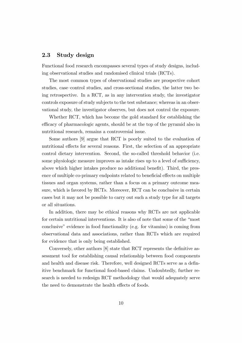
2.3 Study design

Functional food research encompasses several types of study designs, includ-

ing observational studies and randomised clinical trials (RCTs).

The most common types of observational studies are prospective cohort

studies, case—control studies, and cross-sectional studies, the latter two be-

ing retrospective. In a RCT, as in any intervention study, the investigator

controls exposure of study subjects to the test substance; whereas in an obser-

vational study, the investigator observes, but does not control the exposure.

Whether RCT, which has become the gold standard for establishing the

effi cacy of pharmacologic agents, should be at the top of the pyramid also in

nutritional research, remains a controversial issue.

Some authors [9] argue that RCT is poorly suited to the evaluation of

nutritional effects for several reasons. First, the selection of an appropriate

control dietary intervention. Second, the so-called threshold behavior (i.e.

some physiologic measure improves as intake rises up to a level of suffi ciency,

above which higher intakes produce no additional benefit). Third, the pres-

ence of multiple co-primary endpoints related to beneficial effects on multiple

tissues and organ systems, rather than a focus on a primary outcome mea-

sure, which is favored by RCTs. Moreover, RCT can be conclusive in certain

cases but it may not be possible to carry out such a study type for all targets

or all situations.

In addition, there may be ethical reasons why RCTs are not applicable

for certain nutritional interventions. It is also of note that some of the “most

conclusive”evidence in food functionality (e.g. for vitamins) is coming from

observational data and associations, rather than RCTs which are required

for evidence that is only being established.

Conversely, other authors [8] state that RCT represents the definitive as-

sessment tool for establishing causal relationship between food components

and health and disease risk. Therefore, well designed RCTs serve as a defin-

itive benchmark for functional food-based claims. Undoubtedly, further re-

search is needed to redesign RCT methodology that would adequately serve

the need to demonstrate the health effects of foods.

10

3 Surrogate Endpoints

Markers and surrogate endpoints have an increasingly important role in both

clinical and nutritional research. However, the challenges that must be over-

come in their adoption are many, and range from discovery and verification

through to statistical validation, successful use in nutritional epidemiology

studies and, lastly, routine use.

From a statistical standpoint, according to the definitions given in [10]

that best pertain to functional food research, we refer to a validated marker

as one that has been demonstrated by robust statistical methods to fore-

cast the likely response to a dietary intervention (predictive biomarker) or

to be able to replace a clinical endpoint to assess the effect of a relevant

intake of specified food components (surrogate endpoint). Despite the po-

tential of surrogate endpoints, there is no widely accepted agreement about

what constitutes a valid surrogate endpoint. In early discussions about sur-

rogate endpoints, a common misconception was that it was suffi cient for this

endpoint to be prognostic for the clinical endpoint to establish surrogacy.

Different approaches have been taken by researchers to quantify the treat-

ment effect on the clinical outcome explained by the surrogate endpoint: 1)

analysis based on individual patient data (IPD), and 2) meta-regression based

on summary statistics from published literature.

It is widely recognized that by accessing original data, one can enhance

comparability among studies with respect to inclusion/exclusion criteria, de-

finitions of variables, adjustments of covariates, estimation of parameters by

the same statistical method and perform model building and diagnostics [11].

Providing summary statistics is logistically simpler than transferring original

data. Moreover, protection of human subjects and other study policies often

prohibit investigators from releasing IPD.

11

3.1 Validation on individual data

The mathematical construct to a problem that had traditionally been car-

ried out by intuition, was given by Prentice [12] in his landmark paper.

Prentice proposed a formal definition of a surrogate endpoint and suggested

operational criteria for its validation in the case of a single trial and single

surrogate.

Define T and S to be the random variables that denote the true and surro-

gate endpoints, respectively, Z to be a binary indicator variable for treatment

and j the index for the j-th subject enrolled in the study. The endpoints

T and S can be discrete or continuous, possibly censored, random variables.

Prentice’s definition can be written as f(S|Z) = f(S) ⇐⇒ f(T |Z) = f(T ),

where f(·) denotes the probability distribution of random variable and f(·|·)denotes the conditional probability distribution. Note that this definition

involves the triplet (T, S, Z), hence the endpoint S is a surrogate for T only

with respect to the effect of some specific treatment Z, except if S were a

perfect surrogate for T , i.e., if S and T were the same endpoint up to a

deterministic transformation.

According to the definition, a surrogate endpoint is a random variable for

which a test for the null hypothesis of no treatment effect is also a valid test

for the corresponding null hypothesis for the true endpoint.

Prentice proposed four operational criteria to check if a triplet (T, S, Z)

fulfills the definition. Symbolically, they can be written as follows:

f(S|Z) 6= f(S)

f(T |Z) 6= f(T )

f(T |S) 6= f(T )

f(T |S,Z) = f(T |S)

In words, the first criterion states that the surrogate endpoint is associ-

ated with treatment. The second states that the true endpoint is associated

with treatment. The third is that the surrogate and the true endpoints are

associated. The last criterion states that, given the surrogate endpoint, treat-

12

ment and the true endpoint are independent. Popularly, the last criterion is

referred to as the Prentice criterion.

To exemplify as in [13], we consider a formulation for joint modeling of

the endpoints through a bivariate model where the effect of the treatment

on the surrogate is modeled by:

Sj = µS + αZj + εSj (1)

and the effect of the treatment on the true endpoint is modeled by:

Tj = µT + βZj + εTj (2)

and the error terms have a joint zero-mean Normal distribution with variance-

covariance matrix Σ =

(σSS σST

σTT

).

The first two operational criteria require testing the significance of pa-

rameters α and β. The third criterion can be verified using the test for

parameter γ in the model describing the relationship between S and T :

Tj = µ+ γSj + εj (3)

The so-called Prentice criterion is verified through the conditional distri-

bution of T given Z and S:

Tj = µT + βSZj + γZSj + εTj (4)

where βS = β − σSTσ−1SSα and γZ = σSTσ

−1SS and it requires that βS be

non-significant. This raises a conceptual diffi culty.

Freedman, Graubard, and Schatzkin [14] argued that the last Prentice

criterion might be adequate to reject a poor surrogate endpoint (if a test

for treatment effect upon the true endpoint remains statistically significant

after adjustment for the surrogate), but it is inadequate to validate a good

surrogate endpoint, since failing to reject the null hypothesis may be due

merely to insuffi cient power. Therefore, they proposed to use the proportion

of treatment effect explained by the surrogate endpoint as a measure of the

validity of a potential surrogate. A high proportion would indicate that a

13

surrogate is useful.

Let PE(T, S, Z) be for the proportion of the effect of Z on T which can

be explained by S. An estimate of the explained proportion is

PE(T, S, Z) = (β − βS) /β (5)

where β and βS are the estimates of the effect of Z on T , respectively,

without and with adjustment for S. PE being the ratio of two parameters,

its confidence limits can be calculated using Fieller’s theorem or the delta

method [15].

Several authors have pointed towards drawbacks of the measure. For

instance, Buyse and Molenberghs [16] have shown that the proportion of

treatment effect explained by the surrogate is not truly a proportion, as it

can fall out of the [0, 1] interval. As an alternative, Buyse and Molenberghs

[16] proposed to replace the proportion of treatment effect explained by the

surrogate by another set of surrogacy criteria closely related to it: the rel-

ative effect (RE) and the adjusted association (AA). The former, defined

at the population level, is the ratio of the overall treatment effect on the

true endpoint over that on the surrogate endpoint (β/α, under the current

notation). The second one is the individual-level association between both

endpoints, after accounting for the effect of treatment.

Intuitively, RE is a conversion factor between the treatment effect on

the surrogate to that on the primary endpoint. If the multiplicative relation

could be assumed, and if RE were known exactly, it could be used to predict

the effect of Z on T based on an observed effect of Z on S. In practice, RE

will have to be estimated, and the precision of the estimation will be relevant

for the precision of the prediction.

Generically, AA = corr(T |Z, S|Z) is the correlation between the true and

surrogate endpoint after adjusting for the treatment effect. In the previous

example of normally distributed endpoints, AA = σST/√σSSσTT . It follows

that, if AA = 1, one could call the surrogate “perfect at the individual level”,

as the knowledge of S and Z would allow for an exact prediction of the value

of T for an individual subject. In a general situation, it is then important to

14

judge whether the correlation is considered high enough for the surrogate to

be trustworthy.

Another line of research has been in the setting corresponding to a multi-

center trial or a meta-analysis of trials [17]. Thus, the current notation will be

supplemented using index i for the i-th center or trial. A natural formulation

for joint modeling of the endpoints is through a bivariate mixed model:

Sj = µS + αZij +mSi + aiZij + εSij (6)

Tj = µT + βZij +mT i + biZij + εT ij

where µS and µT are fixed intercepts, α and β are the fixed effects of Z on

the endpoints, mSi and mT i are random intercepts and, ai and bi the random

effects of Z on the endpoints in the i-th trial. The correlated error terms εSijand εT ij are assumed to be zero-mean normally distributed with variance-

covariance matrix Σ =

(σSS σST

σTT

)and the vector of random effects is

assumed to be zero-mean normally distributed with variance-covariance ma-

trix:

D =

dSS dST dSA dSB

dTT dTA dTB

dAA dAB

dBB

We denote with θ the vector of fixed-effects parameters and variance

components.

The association between both endpoints after adjustment for the treat-

ment effect is captured by the squared correlation between S and T after

adjustment for both the trial effects and the treatment effect:

R2between-trial = σ2ST/σSSσTT (7)

This aspect of surrogacy is generally referred to as individual-level sur-

rogacy, which means that for individual patients, the marker or surrogate

outcome must correlate well with the final endpoint of interest. It general-

izes AA to the case of several trials.

15

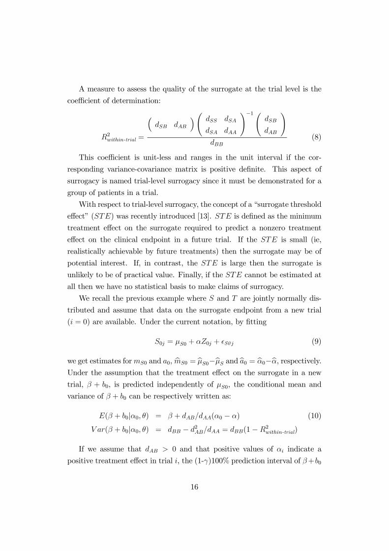
A measure to assess the quality of the surrogate at the trial level is the

coeffi cient of determination:

R2within-trial =

(dSB dAB

)( dSS dSA

dSA dAA

)−1(dSB

dAB

)dBB

(8)

This coeffi cient is unit-less and ranges in the unit interval if the cor-

responding variance-covariance matrix is positive definite. This aspect of

surrogacy is named trial-level surrogacy since it must be demonstrated for a

group of patients in a trial.

With respect to trial-level surrogacy, the concept of a “surrogate threshold

effect”(STE) was recently introduced [13]. STE is defined as the minimum

treatment effect on the surrogate required to predict a nonzero treatment

effect on the clinical endpoint in a future trial. If the STE is small (ie,

realistically achievable by future treatments) then the surrogate may be of

potential interest. If, in contrast, the STE is large then the surrogate is

unlikely to be of practical value. Finally, if the STE cannot be estimated at

all then we have no statistical basis to make claims of surrogacy.

We recall the previous example where S and T are jointly normally dis-

tributed and assume that data on the surrogate endpoint from a new trial

(i = 0) are available. Under the current notation, by fitting

S0j = µS0 + αZ0j + εS0 j (9)

we get estimates formS0 and a0, mS0 = µS0−µS and a0 = α0−α, respectively.Under the assumption that the treatment effect on the surrogate in a new

trial, β + b0, is predicted independently of µS0, the conditional mean and

variance of β + b0 can be respectively written as:

E(β + b0|α0, θ) = β + dAB/dAA(α0 − α) (10)

V ar(β + b0|α0, θ) = dBB − d2AB/dAA = dBB(1−R2within-trial)

If we assume that dAB > 0 and that positive values of αi indicate a

positive treatment effect in trial i, the (1-γ)100% prediction interval of β+b0

16

can be expressed as:

E(β + b0|α0, θ)± z1−γ/2√V ar(β + b0|α0, θ) (11)

where z1−γ/2 is the quantile 1 − γ/2 of the standard normal distribution.

The lower and upper limit of this interval, l(α0) and u(α0), respectively, are

functions of α0.The value of α0 such that l(α0) = 0 is the STE.

Many advocate that results from studies where only the surrogate is ob-

served should never be considered definitive. As a consequence, several meth-

ods have been proposed for augmented surrogate endpoints. Such methods

assume that there is a sample where complete information on the surrogate,

primary endpoint and covariates are observed, and a sample where the pri-

mary endpoint cannot be observed and only information on the surrogate

and the covariates are available. This is data coarsening [18], a generalized

concept of missingness. According to a recent review [19], these methods

encompass likelihood-based approaches assuming a full parametric model for

the joint distribution for (T, S) and requiring few assumption on coarsen-

ing; non-likelihood approaches where the lack of a full specification on the

joint distribution for (T, S) is compensated by stronger assumptions on the

coarsening mechanisms; and non-likelihood based methods making just some

assumptions on the joint distribution of (T, S). Although there is not a single

overall best method, in general the gains in using augmented surrogate end-

point approaches is high only if S is a good correlate for T and if the amount

of missing assessments of the primary endpoint is moderate or high [19].

The mechanism that governs this missingness (i.e. at random, completely at

random,. . . ) is crucial in all the methods.

More recent research has been utilizing ideas of causal inference to the

assessment of surrogacy. The first approach was described by Robins and

Greenland [20]. In their work, the surrogate endpoint is an intermediate

variable measured after the baseline covariates and before the outcome. This

variable is manipulable and can affect the outcome independently of the

treatment. From the causal viewpoint towards surrogacy, it is crucial to

be able to formulate appropriate causal pathways in considering the effects

17

of a treatment on a surrogate and the true endpoint. This underscore the

necessity in enhancing understanding of the biological role of surrogates on

mechanisms by which food components positively affect health. Figure 1

shows a valid pathway for a surrogate endpoint.

time

Healthcondition

Surrogateendpoint

True clinicalendpoint

Dietaryintervention

Figure1: Paradigm for valid surrogate endpoint

Lassere [21] has proposed a formal schema for numerically assessing the

strength of the relationship between S and T , based on a weighted evalu-

ation of biological, epidemiological, statistical, clinical trial and risk-benefit

evidence.

3.2 Validation on summary statistics: a meta-analysis

perspective

The basic situation in meta-analysis is that we are dealing with n studies

in which a parameter of interest is estimated. In a meta-analysis of clinical

trials the parameter is a measure of the difference in effi cacy between the two

treatment arms. Combination of estimates is usually achieved using one of

two assumptions, yielding a fixed-effect or random-effects meta-analysis (see

[22] for a review).

Methods based on the mathematical assumption that a single common

(or ’fixed’) effect underlies every study in the meta-analysis are referred to

as fixed effect meta-analyses. Methods that assume individual studies to es-

timate different true treatment effects are referred to as random-effect met-

analyses. Another term for such between-study variation is heterogeneity.

18

Prior to performing a meta-analysis, it customary to test for heterogene-

ity. In general, Q test [23] is computed by summing the squared deviations of

each study’s effect estimate from the combined effect estimate, weighting the

contribution of each study by its inverse variance. It is well recognized that

the power of this test is low and that may be preferable to know the extent of

true heterogeneity. The I2 statistic [24] accomplishes this task by describing

the percentage of variation in effect estimates that is due to heterogeneity.

There is a great deal of debate about whether it is better to use a fixed or

random effect meta-analysis. The debate is not about whether the underlying

assumption of a fixed effect is likely but more about which is the better

trade off, stable robust techniques with an unlikely underlying assumption

or less stable techniques based on a somewhat more likely assumption. The

random-effects method has long been associated with problems due to the

poor estimation of among-study variance when there is little information.

In contrast to simple meta-analysis, combinations of meta-analytic princi-

ples with regression ideas (of predicting study effects using study-level covari-

ates) have been developed, namely meta-regressions. Meta-regression aims

to relate the size of effect to one or more study-level characteristics. It is

appropriate to use meta-regression to explore sources of heterogeneity even

if an initial overall Q test for heterogeneity is non-significant. Some would

argue that, given the diversity of trials in any meta-analysis, that hetero-

geneity must exist and whether we happen to be able to detect it or not is

irrelevant.

The outcome (or dependent) variable in a meta-regression analysis is

usually a summary statistic, for example the observed log odds ratio from

each trial. The estimated variance of this summary statistic is assumed to be

the true variance, an assumption that is questionable when trials are small.

Under a fixed-effect meta-regression model, we may assume that the ob-

served log odds ratio (yi) are independently normally distributed as:

yi ∼ N(φ+ γxi, ν2i ) (12)

where ν2i is the variance of the log odds ratio and xi denotes the covariate

19

value in the i-th trial.

Maximum Likelihood (ML) estimates may be obtained by ordinary least

squares with weights wi = 1/ν2i . This method is known as Weighted Least

Squares (WLS) regression. The ratio between Pearson goodness-of-fit χ2

and the model degrees of freedom, provides an estimate of the overdispersion

parameter. This give indications of residual heterogenity and can be thought

as a multiplicative factor for ν2i .

Heterogeneity can be incorporated in a meta-regression model by adding

to (12) a between-study variance component (τ 2) that represents the excess

variation in observed effects over that expected from within-study variation:

yi ∼ N(φ+ γxi, ν2i + τ 2) (13)

ML estimates may be obtained by ordinary least squares with weights

wi = 1/(ν2i + τ 2). τ 2 must be explicitly estimated in order to undertake the

weighted regression and this is somewhat problematic. Different estimates

have been advocated such as restricted ML (REML) estimate and the em-

pirical Bayes estimate. Methods which use the binomial model for observed

proportions rather than assuming normality of the log-odds ratios, though

preferable in principle, often give similar results in practice [25].

When the independent variable in a meta-regression represents a dose or

exposure level and summarized data are reported as a series of dose-specific

odds ratios, with one category serving as the common referent group, the

WLS method to trend estimation is no longer suitable. Greenland and Long-

necker [26] suggested the use of Generalized Least Squares (GLS) to allow for

the correlation between log odds ratios. This method is then incorporated

in the estimation of fixed and random-effects meta-regression models for the

analysis of multiple studies.

The correlation between yjk and yjl, the k-th and l-th log odds ratio in

the i-th study, is ri,kl = vi0/√

(vikvil), where for i 6= k, vi0 = 1/Ci0 + 1/Di0

and vik = 1/Ci0 + 1/Di0 + 1/Cik + 1/Dik, being (Ci0;Di0) and (Cik;Dik) the

numbers of cases and controls, respectively, for the unexposed group (x = 0)

and the exposed group with assigned dose xik. Assuming that the log odds

20

ratio in the unexposed group (reference category) is zero, no intercept models

are used.

Adaptations to this method for trend estimation that allow for both cor-

relation between log odds ratios and arbitrarily aggregated dose-levels have

been implemented [27].

The criteria for surrogacy given in the previous section, except those

defined at individual-level, may be assessed on summary statistics via meta-

regression although several limitations of this approach must be recognized.

The associations derived from meta-regressions are observational, although

the original studies may be randomized trials, and have a weaker interpre-

tation than the causal relationships derived from randomized comparisons.

This applies particularly when averages of patient characteristics in each

study are used as covariates in the regression since the relationship with pa-

tient averages across studies may not be the same as the relationship for

patients within studies (ecological bias) [28]. Furthermore a meta-regression

approach will typically have lower power than an IPD meta-analysis.

IPD, both of outcomes and covariates, can alleviate some of the problems

in meta-regression. In particular within-trial and between-trial relationships

can be more clearly distinguished, and confounding by individual level co-

variates can be investigated. Nevertheless many of the problems remain, not

least those related to data dredging, the main pitfall in reaching reliable con-

clusions from meta-regression. It can only be avoided by prespecification of

covariates that will be investigated as potential sources of heterogeneity [28].

21

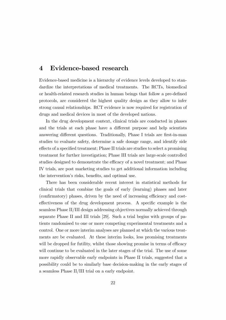
4 Evidence-based research

Evidence-based medicine is a hierarchy of evidence levels developed to stan-

dardize the interpretations of medical treatments. The RCTs, biomedical

or health-related research studies in human beings that follow a pre-defined

protocols, are considered the highest quality design as they allow to infer

strong causal relationships. RCT evidence is now required for registration of

drugs and medical devices in most of the developed nations.

In the drug development context, clinical trials are conducted in phases

and the trials at each phase have a different purpose and help scientists

answering different questions. Traditionally, Phase I trials are first-in-man

studies to evaluate safety, determine a safe dosage range, and identify side

effects of a specified treatment; Phase II trials are studies to select a promising

treatment for further investigation; Phase III trials are large-scale controlled

studies designed to demonstrate the effi cacy of a novel treatment; and Phase

IV trials, are post marketing studies to get additional information including

the intervention’s risks, benefits, and optimal use.

There has been considerable recent interest in statistical methods for

clinical trials that combine the goals of early (learning) phases and later

(confirmatory) phases, driven by the need of increasing effi ciency and cost-

effectiveness of the drug development process. A specific example is the

seamless Phase II/III design addressing objectives normally achieved through

separate Phase II and III trials [29]. Such a trial begins with groups of pa-

tients randomised to one or more competing experimental treatments and a

control. One or more interim analyses are planned at which the various treat-

ments are be evaluated. At these interim looks, less promising treatments

will be dropped for futility, whilst those showing promise in terms of effi cacy

will continue to be evaluated in the later stages of the trial. The use of some

more rapidly observable early endpoints in Phase II trials, suggested that a

possibility could be to similarly base decision-making in the early stages of

a seamless Phase II/III trial on a early endpoint.

22

Not all intervention programmes are candidates for these designs, partic-

ularly if complex treatment regimens are involved and a long follow-up time

to assess the surrogate is needed [30].

Methods for the use of early endpoint data based on the group-sequential

approach have been proposed in settings where the correlation between the

endpoints can be assumed known or estimated from data on both endpoints

from an interim analysis, or based on the combination test approach when

no primary endpoint data are available at the interim analysis. In both ap-

proaches, it is a challenge to determine sample size for achieving the desidered

power and to carry out a valid final analysis combining data from both phases.

The use of an early endpoint at the interim analysis and of a primary

endpoint at a later analysis on the same patients, leads to potential type

I error inflation due to correlation between the two endpoints. The basic

idea behind group sequential designs is to avoid excessive false conclusions

by using much lower significance levels than the overall α at each interim

analysis.

In a classical design, the test statistic S (i.e. a t-test, a Chi-square test

or a z-test depending on the response variable chosen as the trial endpoint),

is used to derive the probability of rejection of the null or the alternative hy-

pothesis. Such exercise is performed once, at the end of the study enrolment

and outcome evaluation.

In a one-sided group sequential test, such exercise is repeated at each

k-th interim analysis, k=1,. . . ,K. In this case, the test statistics Sk that are

appropriate for the type of response data being monitored are compared with

boundary values lk and uk:

• if Sk > uk, the trial will be stopped with the null hypothesis rejected

in favour of the one-sided alternative;

• if Sk > lk, the trial will be stopped and the null hypothesis will not be

rejected;

• if lk < Sk < uk the trials continues to the (k+1)-th interim analysis.

23

Here l1, u1,. . . , lK , uK are constants with lK < uK for k=1,. . . ,K-1

and lK = uK in order to ensure a final decision. These stopping limits are

chosen to control the type I error probability, i.e., P (S1 > u1 or . . . or SK >

uK) = α. The nominal significance level at the k-th analysis is defined as

the marginal probability αk= P (SK > uK) and should not be confused with

the probability πk of stopping at stage k and rejecting the null hypothesis,

πk = P (l1 < S1 < u1, . . . , lk−1 < Sk−1 < uk−1, Sk > uk). Since π1 + . . . +

πK = α, πk is sometimes referred to as the error spent at stage k.

The values of lk and uk can be obtained via a recursive numerical inte-

gration technique first described by Armitage et al [31]. Further details are

given by Jennison and Turnbull [32].

An alternative approach to analysing data at interim analyses, is the

combination test approach proposed by Bauer and Köhne [33]. The origin

of this procedure lies in Fisher combination test which combines the one-

sided p-values p1 and p2 from the two separate stages of the trial through

an appropriate function. The null hypothesis is rejected if p1p2 <l2 = exp(-

1/2χ24,α) where χ24,α is the 100(1-α)-th percentile of a Chi-square distribution

with four degrees of freedom. To stop the trial for futility, a lower bound for

p1, α0, must be specified. To get an overall α-level test, a value α1 > l2 has

to be determined.

The application of the combination test can be summarized as follows:

• if p1 > α0, the trial will be stopped and the null hypothesis will not be

rejected (stopping for futility);

• if p1 < α1, the trial will be stopped and the null hypothesis will be

rejected;

• if α1 < p1 < α0 the trials continues to the second stage.

Alternatively, the independent test statistics from the different stages

of the trial can be combined directly [34]. These two types of adaptive

procedures have been compared by Wassmer [35].

24

4.1 Evidence-based nutrition

During the last decade, approaches to evidence-based medicine, have been

adapted to nutrition science and policy. However, there are distinct differ-

ences between the evidence that can be obtained for the testing of drugs using

RCTs and those needed for the development of nutrient requirements or di-

etary guidelines. Although RCTs present one approach toward understand-

ing the effi cacy of nutrient interventions, the innate complexities of nutrient

actions and interactions cannot always be adequately addressed through any

single research design [36].

The difference we focus on is between endpoints.

While drugs acts promptly and their endpoint can be measured over rel-

atively short periods of time, nutrients effects tend to manifest themselves

in small differences over long periods of time. This is the reason why the

use of surrogate endpoints is particularly relevant for functional food re-

search. Although the motivation for using seamless designs incorporating

short-term and long-term endpoints may be shared by evidence-based medi-

cine and evidence-based nutrition, the unavailability of the true endpoint

even at later stages of the trial, makes such methods not completely fit to

functional food research.

Our proposal is to adapt to the functional food context the method devel-

oped by Chow [37] for a two-stage seamless designs. In his work he proposed a

test statistic for the final analysis, based on combined data from the learning

phase and the confirmatory phase of a seamless Phase II/III trial, assuming

an established linear relationship between the two different study endpoints.

Similarly, under a relationship between the surrogate and the true endpoint,

established in the surrogacy assessment, we derive design considerations, in

terms of sample size and power of a test on the true endpoint based on its

conditional variance.

4.2 Continuos data

Suppose the investigators are planning a single arm Phase II study to evaluate

activity of a dietary intervention on a validated surrogate endpoint S.

25

Let us assume that Sj are independently and normally distributed random

variables with mean µ unknown and variance ξ2 known. The following null

(H0) and alternative hypotheses (H1) are considered:

H0 : µ = γ0 vs. H1 : µ = γ1 (γ1 > γ0)

The sample size nS1 determined such that the corresponding α-level test

would achieve a fixed (1-β) power is:

nS1 =(z1−β − zα/2)2ξ2

(γ1 − γ0)2(14)

where z1−β and zα/2 are the quantiles 1 − β and α/2, respectively, of the

standard normal distribution.

Suppose that S is a valid surrogate endpoint for the true endpoint T and

they can be related by the following relationship (as in equation (3)):

Tj = φ+ γSj + εj (15)

We assume that this relationship is well-explored, φ and γ are known, and

εj are zero-mean normally distributed error terms with variance σ2. We recall

that the assessment of the third Prentice’s criterion for surrogacy requires

the exploration of this relationship through a the test for parameter γ.

Even though T is unobservable, the investigators may be interested in

linking a test on S with a test on T with the same power and α level, both

in terms of hypotheses specification and sample size.

Let us define a generic set of hypotheses for a one-sample test on the

mean of T :

H0 : µ = µ0 vs. H1 : µ = µ1 (µ1 > µ0)

By replacing µ1 with the predicted value of T at Sj = γ1, µ1, in the following

equation :γ1 − γ0

ξ=µ1 − µ0

σ(16)

we get µ0 = µ1 + (γ0−γ1)σξ

.

Therefore, the sample size nT1, as a function of the value of µ1, determined

26

such that the corresponding α-level test would achieve the fixed (1-β) power

is:

nT1 =(z1−β − zα/2)2σ2[µ1 − µ1 + (γ1−γ0)σ

ξ

]2 (17)

that can be rewritten as:

nT1 = nS1(γ1 − γ0)2σ2

[(µ1 − µ1)ξ + (γ1 − γ0)σ]2(18)

The same connection can be made between the sample size nS1 and the

sample size for a Phase III trial with two balanced arms, A and B, with T

as primary endpoint, say nT2. In this case the set of hypotheses is:

H0 : µA − µB = 0 vs. H1 : µA − µB = µ1 − µ0 (> 0)

Assuming that the variance σ2 is the same in both arms and recalling

that nT2 = 4nT1 (with the same power and α level), nT2 may be rewritten

as:

nT2 = nS1(γ1 − γ0)24σ2

[(µ1 − µ1)ξ + (γ1 − γ0)σ]2(19)

Suppose the investigators are planning a two-arm Phase III study to

evaluate effi cacy of a dietary intervention on a validated surrogate endpoint

S, with the same variance ξ2 in both arms with:

H0 : µA − µB = 0 vs. H1 : µA − µB = γ1 − γ0 (> 0)

Directly from equation (18), it follows:

nT2 = nS2(γ1 − γ0)2σ2

[(µ1 − µ1)ξ + (γ1 − γ0)σ]2(20)

These results are summarized in Table 4 and can be extended to the case

of unknown variance by referring to a t-test rather than a z-test. Obviously,

by setting µ1 = µ1, nT1 = nS1 and nT2 = nS2. This means that the same

sample size that provides a fixed power for an α-level test on the difference

of means γ1 − γ0 on the surrogate, also provides the same power for an α-level test on the difference (γ1 − γ0)σ/ξ on the true endpoint. The joint

27

consideration of these two sets of hypotheses, one on the surrogate and the

other on the true endpoint, helps orienting the investigators and, hopefully,

discourages studies on the surrogate that would allow to test only unrealistic

effects on the true endpoint.

Surrogate\True Phase II Phase III

Phase II nT1=nS1(γ1−γ0)2σ2

[(µ1−µ1)ξ+(γ1−γ0)σ]2nT2=nS1

(γ1−γ0)24σ2[(µ1−µ1)ξ+(γ1−γ0)σ]2

Phase III - nT2=nS2(γ1−γ0)2σ2

[(µ1−µ1)ξ+(γ1−γ0)σ]2

Table 4. Sample size of a single-arm Phase II (nT1) trial and two-arm Phase

III (nT2) trial for the true endpoint as a function of the sample sizes for the surro-

gate endpoint under equation (13). Power and two-sided α-level are the same for

all study designs.

4.3 Validation of a prognostic model

In medical research, regression models for investigating patient outcome in

relation to patient and disease characteristics as in (15) are termed prognostic

models.

According to the definition given by Altman [38], a statistically validated

prognostic model is one which passes all appropriate statistical checks, in-

cluding goodness-of-fit on the original data and unbiased prediction on new

data.

One common way of establishing how well a model might perform for

further patients is data splitting or cross-validation. Here the original sample

is split into two parts before the modelling begins. The model is derived on

the first portion of the data (often called the training set) and then its ability

to predict outcome is evaluated on the second or test data set. A variation

is to carry out the modelling procedure on each portion of the data and to

evaluate each model on the other portion.

An issue is how to split the data set. Although cross-validation is widely

recommended, authors rarely consider what proportion of patients should

be in the test and training sets (or fail to justify any recommendation).

28

Random splitting must lead to data sets that are the same other than for

chance variation and is thus a weak procedure. Furthermore, estimates of

predictive accuracy from data-splitting procedures, though unbiased, tend to

be imprecise (see Efron and Tibshirani [39]).

A tougher test is to split the data in a non-random way. For example,

we might take groups of patients seen in different time periods. Rather

different, and better, approaches are to use bootstrapping or leave-one out

cross-validation. From these analyses shrinkage factors can be estimated and

applied to the regression coeffi cients to counter overoptimism (see Harrell

[40]).

In the case of univariable ordinary least squares regression we can define

the ordinary predictor for any value s of S as µ = T + (S− s)γ, where T andS are the sample mean of T and S, respectively.

Van Houwelingen and Le Cessie [41] suggest shrinking this ordinary pre-

dictor in dependence on a shrinkage factor c. The resulting predictor is then

defined by µS = T + (S − s)cγ. Furthermore they suggest to estimate theshrinkage factor c by cross- validation which is performed in the following

way: for each individual j of the sample the estimate γ−1 based on all indi-

viduals except j is computed. Next for each individual the linear predictor

ηj = φ+ sj γ−1 is computed. Then a generalized linear model with Tj and ηjas dependent and independent variable, respectively, is fitted to the obser-

vations. The regression coeffi cient c obtained is then taken as the shrinkage

factor, resulting in a new predictor µS, preferable to the ordinary predictor

with respect to the expected average prediction error.

As we would expect to predict a variation on the true enpoint for future

patients consequent upon a variation on the surrogate, attention to the issue

of overoptimistic prediction in (15) should be paid.

29

5 Surrogate Endpoint for Cardiovascular Risk

Reduction: a case-study

CVD, a major cause of death in Western populations and a constantly grow-

ing cause of morbidity and mortality worldwide, can be prevented by lifestyle

changes, one of which is diet [42].

Numerous potential surrogate endpoints of CVD are being evaluated as

the pathophysiology of heart disease is becoming better understood. Func-

tional foods marketed with the claim of reduction of heart disease risk often

focus on these surrogates.

High cholesterol concentration is a well-established risk factor for CVD as

it can lead to atherosclerotic plaque formation, which can lead to a narrowing

of the coronary arteries. Atherosclerotic plaques can rupture and lead to a

heart attack or a stroke. Primary prevention trials using cholesterol-lowering

drugs and dietary interventions have shown that lowering blood cholesterol

can reduce the risk of myocardial infarction and death from CHD. Elevated

blood cholesterol concentration has been associated with increased risk of

CVD in several observational studies [43].

For example, the FDA used blood total cholesterol concentration as a

surrogate endpoint for CVD risk to substantiate several authorized health

claims: 1) saturated fat and cholesterol and increased risk of CHD, 2) fruits,

vegetables, and grain products that contain fiber (particularly soluble fiber)

and reduced risk of CHD, 3) soluble fiber from certain foods and reduced

risk of CHD, 4) soy protein and reduced risk of CHD, and 5) stanols/sterols

and reduced risk of CHD. In addition, three health claims based on credible

scientific evidence, the so-called qualified health claims, were issued based on

studies using blood total cholesterol as a surrogate endpoint. These claims

include the following: 1) unsaturated fatty acids from canola oil and reduced

risk of CHD, 2) monounsaturated fatty acids from olive oil and reduced risk

of CHD, and 3) corn oil and products containing corn oil and reduced risk

30

of heart disease.

5.1 Methods

Surrogacy assessment.

The meta-analyses by Gould et al. [44-46] contributed to the validation of

total cholesterol as a surrogate endpoint for CVD.

Using the 27 trials included in [45] that regard a unifactorial primary

or secondary intervention classified as “Diet/Other”or “Statin”, we verified

Prentice criteria for surrogacy under a random-effect metanalysis perspective.

The CHD mortality log odds ratio (CHDlogOR) is the true endpoint and

the net improvement in percentage cholesterol reduction (%ChRed) is the

surrogate endpoint.

The within-study variance of %ChRed was not reported in [45], there-

fore we used an approximation to verify the first criterion, by calculating

the weighted mean of %ChRed using the same inverse variance weights for

CHDlogOR.

The other criteria were verified through random-effect meta-regression

analyses, assuming a normal distribution for the residuals (as in (13)) and dif-

ferent predictors (intercept only, average within-study %ChRed, and average

within-study %ChRed and treatment, respectively). REML and empirical

Bayes estimates of τ 2 were considered.

The data are given in Table 5. The odds ratio of CHD is the summary

of the results in each trial. Each odds ratio is estimated as the cross-product

of cell counts in the corresponding 2x2 contingency table, with the variance

of the log-odds ratio equal to the sum of the reciprocal cell counts, as usual.

In the trials with no events in one group, 0.5 is added to each cell for these

calculations.

On the basis of the investigated relation between CHDlogOR and%ChRed

we make sample size considerations for a test on means between two groups.

31

Intervention %ChRed CHD deaths/NI CHD deaths/NCDiet/Other 9 32/1906 44/1900

9.8 19/1149 31/1129

12.7 41/424 50/422

23.3 33/421 41/417

14 13/77 23/143

9.9 238/1119 632/2789

4 97/1018 97/1015

4.3 37/221 24/237

8.3 17/123 20/129

8.8 8/54 1/26

13.5 25/199 25/194

13.9 37/206 50/206

30.3 NA NA

19.1 NA NA

12.2 1/26 3/28

23.3 0/24 3/28

16 NA NA

22 NA NA

Statin 20 41/3302 61/3293

26 111/2221 189/2223

20 96/2081 119/2078

12.1 2/76 4/75

20 0/460 6/459

31 NA NA

20 2/168 1/166

22 4/193 4/188

20 10/955 12/936

Table 5. Trials included in [45] being "Diet/Other" or "Statin" the interventions.

NI : sample size of the intervention arm, NC : sample size of the control arm, NA:

data not available.

32

Simulation study.

The scenario chosen for simulation aims to represent the investigated relation

between CHDlogOR and %ChRed where an hypothetical shrinkage factor of

0.8 (with an assigned between-study distribution) is applied to correct for

overestimation of the conditional expectation of CHDlogOR.

The individual value of CHDlogOR (Ti) as a function of %ChRed (Si)

was generated for 50 studies according to the relation Ti = γSici + εi,

where Si and εi were from a Normal with mean equal to 14 and variance

ξ2 =49 and a zero-mean Normal with two different choices for the variance

σ2: 0.04 and 0.64, respectively. Two different values of the regression coeffi -

cient γ were chosen, namely -0.017 and -0.17, and three different shrinkage

(ci) mechanisms were considered: ci generated according to a Gamma with

mean 0.8 and variance σ2S =0.01, σ2S =0.04 or σ2S =0.1, respectively. This

means that a factor of 0.8 is needed to correct for overestimation of the

conditional expectation of CHDlogOR and the conditional variance, now de-

pending on the value taken by %ChRed, is increased.

The sample size to achieve a 80% or a 90% power for a two-sided (α = 5%)

test on the difference of means (µA−µB) of %ChRed was calculated accord-ing to formulas given in subsection 4.1, assuming ξ2 = 49 and under different

alternative hypotheses: µA − µB = 1, µA − µB = 1.5, µA − µB = 2 and

µA − µB = 5. On the basis of the surrogacy results, corresponding hypothe-

ses formulation for a test on the difference of means of CHDlogOR were

derived (see Table 6).

Finally, the Monte Carlo experiment was conducted by estimating the power

of a test with effect size and sample size as in Table 6 under known (het-

eroschedastic) variance ((%ChRed·γ)2σ2S + σ2) due to shrinkage for each de-

picted scenario, each with 1000 runs, using the default random number gener-

ating functions in R software. Monte Carlo statistics such as the mean power

and the mean square error (MSE), which equals the mean of the squared

difference between estimated and true power in each simulation, were calcu-

lated.

33

%ChRed CHDlogOR (σ2=0.04) CHDlogOR (σ2=0.64) n80%S2 n90%S2

1 0.029 (OR=1.03) 0.114 (OR=1.12) 1542 2062

1.5 0.043 (OR=1.04) 0.171 (OR=1.19) 686 918

2 0.057 (OR=1.06) 0.229 (OR=1.26) 388 518

5 0.143 (OR=1.15) 0.571 (OR=1.77) 64 86

Table 6. Sample size (npowerS2 ) of a two-arm Phase III trial testing the difference

of means for % Net cholesterol reduction (%ChRed) with ξ2=49 and correspond-

ing hypotheses formulation for a Phase III trial for mean CHDlogOR with the

same sample size and known variance σ2=0.04 or σ2=0.64. Power=0.8 or 0.9 and

two-sided α=0.05. OR: Odds Ratio.

5.2 Results

Surrogacy assessment.

The estimate of the mean %ChRed is 10.7 with 95% Confidence Interval

(95%CI) equal to 7.6-13.8 and 21.9 (95%CI: 19.1-24.7) for “Diet/Other”and

“Statin”, respectively (first criterion verified). The estimate of the mean

CHDlogOR is -0.115 (95%CI: -0.227; -0.003) and -0.41 (95%CI: -0.570; -

0.250) for “Diet/Other”and “Statin”, respectively (second criterion verified).

For one unit increase in %ChRed, the estimated mean of CHDlogOR is -0.026

(95%CI: -0.039; -0.013) (third criterion verified) and the intercept is 0.159

(95%CI: -0.047; 0.365). The trend estimate (model without intercept) is

-0.017 (95%CI: -0.023; -0.011) as shown in Figure 2.

After adjustment for %ChRed, the treatment effect (“Statin”vs. “Diet/

Other”) on CHDlogOR is 0.09 (95%CI: -0.252 ; 0.440) (Prentice criterion

verified).

The fact that a common slope applies for both interventions implies that

there is no evidence to conclude that CHD mortality risk reduction is any-

thing other than proportional to net reduction in cholesterol.

The REML and empirical Bayes estimates of τ 2 were equal to zero for all

models therefore the results of the random-effects meta-regression reduce to

those of the fixed-effect model.

34

­3­2

­10

12

CH

D m

orta

lity 

log(

Odd

s R

atio

)

5 10 15 20 25 30Net Improvement in % Cholesterol Reduction

®

Figure 2: Observed CHDlogOR and predicted regression line relating CHDlogOR

and %ChRed. The area of each circle is inversely proportional to the variance of

the CHDlogOR.

Simulation study.

The results of the simulation study for power=80% are shown in Tables 7a

and 7b and those for power=90% are shown in Tables 8a and 8b.

When the effect of %ChRed is small (γ=-0.017) the effect of shrinkage on

power is negligible, regardless of its variance σ2S.

For increasing values of γ, a test relying on nS2 is underpowered.

The higher the hypothesized difference in means of CHDlogOR and the

shrinkage variance σ2S, the larger the extent of underpowering. This effect is

inversely related to σ2. For example, given an estimated reduction of CHDlo-

gOR of -0.17 for one unit increase in %ChRed and a shrinkage with σ2S = 0.1,

the power of a test to detect a difference of means of CHDlogOR equal to

0.143 (corresponding to σ2 = 0.04) on 64 subjects (32 per arm), would be

reduced from 80% to 39% (Table 7a). This reduction would be smaller, from

80% to 76%, for a larger variance σ2 = 0.64 (Table 7b).

35

Shrinkage Effect (γ) %ChRed CHDlogOR Power MSE

Gamma -0.017 1 0.029 0.800 0.025

σ2S = 0.01 1.5 0.043 0.799 0.024

2 0.057 0.801 0.024

5 0.143 0.801 0.025

-0.17 1 0.029 0.797 0.025

1.5 0.043 0.793 0.026

2 0.057 0.790 0.027

5 0.143 0.736 0.072

Gamma -0.017 1 0.029 0.800 0.025

σ2S = 0.04 1.5 0.043 0.799 0.024

2 0.057 0.801 0.025

5 0.143 0.799 0.024

-0.17 1 0.029 0.789 0.028

1.5 0.043 0.774 0.037

2 0.057 0.757 0.052

5 0.143 0.573 0.230

Gamma -0.017 1 0.029 0.800 0.025

σ2S = 0.1 1.5 0.043 0.799 0.024

2 0.057 0.800 0.024

5 0.143 0.796 0.026

-0.17 1 0.029 0.772 0.039

1.5 0.043 0.738 0.069

2 0.057 0.696 0.108

5 0.143 0.390 0.410

Table 7a. Power of a two-sided (α = 5%) test on CHDlogOR with heteroschedas-

tic variance due to shrinkage and sample size equal to the one of a 80% powered

test on CHDlogOR with variance σ2=0.04. MSE: mean square error.

36

Shrinkage Effect (γ) %ChRed CHDlogOR Power MSE

Gamma -0.017 1 0.114 0.801 0.025

σ2S = 0.01 1.5 0.171 0.799 0.024

2 0.229 0.801 0.025

5 0.571 0.801 0.025

-0.17 1 0.114 0.800 0.025

1.5 0.171 0.800 0.024

2 0.229 0.800 0.027

5 0.571 0.799 0.072

Gamma -0.017 1 0.114 0.800 0.025

σ2S = 0.04 1.5 0.171 0.800 0.024

2 0.229 0.801 0.025

5 0.571 0.802 0.024

-0.17 1 0.114 0.800 0.025

1.5 0.171 0.799 0.025

2 0.229 0.798 0.026

5 0.571 0.786 0.030

Gamma -0.017 1 0.114 0.800 0.025

σ2S = 0.1 1.5 0.171 0.800 0.025

2 0.229 0.803 0.025

5 0.517 0.800 0.026

-0.17 1 0.114 0.799 0.025

1.5 0.171 0.796 0.025

2 0.229 0.794 0.026

5 0.571 0.760 0.049

Table 7b. Power of a two-sided (α = 5%) test on CHDlogOR with heteroschedas-

tic variance due to shrinkage and sample size equal to the one of a 80% powered

test on CHDlogOR with variance σ2=0.64. MSE: mean square error.

37

Shrinkage Effect (γ) %ChRed CHDlogOR Power MSE

Gamma -0.017 1 0.029 0.900 0.018

σ2S = 0.01 1.5 0.043 0.900 0.018

2 0.057 0.900 0.018

5 0.143 0.905 0.019

-0.17 1 0.029 0.898 0.018

1.5 0.043 0.895 0.019

2 0.057 0.891 0.021

5 0.143 0.854 0.051

Gamma -0.017 1 0.029 0.900 0.018

σ2S = 0.04 1.5 0.043 0.900 0.018

2 0.057 0.900 0.101

5 0.143 0.903 0.018

-0.17 1 0.029 0.892 0.020

1.5 0.043 0.882 0.027

2 0.057 0.867 0.039

5 0.143 0.704 0.198

Gamma -0.017 1 0.029 0.900 0.018

σ2S = 0.1 1.5 0.043 0.900 0.018

2 0.057 0.899 0.102

5 0.143 0.900 0.018

-0.17 1 0.029 0.880 0.028

1.5 0.043 0.853 0.052

2 0.057 0.816 0.088

5 0.143 0.500 0.401

Table 8a. Power of a two-sided (α = 5%) test on CHDlogOR with heteroschedas-

tic variance due to shrinkage and sample size equal to the one of a 90% powered

test on CHDlogOR with variance σ2=0.04. MSE: mean square error.

38

Shrinkage Effect (γ) %ChRed CHDlogOR Power MSE

Gamma -0.017 1 0.114 0.900 0.019

σ2S = 0.01 1.5 0.171 0.900 0.018

2 0.229 0.901 0.018

5 0.571 0.905 0.018

-0.17 1 0.114 0.900 0.019

1.5 0.171 0.900 0.018

2 0.229 0.900 0.018

5 0.571 0.902 0.017

Gamma -0.017 1 0.114 0.900 0.019

σ2S = 0.04 1.5 0.171 0.900 0.018

2 0.229 0.901 0.018

5 0.571 0.905 0.018

-0.17 1 0.114 0.899 0.019

1.5 0.171 0.899 0.018

2 0.229 0.899 0.018

5 0.571 0.893 0.020

Gamma -0.017 1 0.114 0.900 0.019

σ2S = 0.1 1.5 0.171 0.900 0.018

2 0.229 0.900 0.018

5 0.517 0.905 0.018

-0.17 1 0.114 0.899 0.019

1.5 0.171 0.897 0.018

2 0.229 0.896 0.019

5 0.571 0.875 0.032

Table 8b. Power of a two-sided (α = 5%) test on CHDlogOR with heteroschedas-

tic variance due to shrinkage and sample size equal to the one of a 90% powered

test on CHDlogOR with variance σ2=0.64. MSE: mean square error.

39

5.3 Discussion

The joint consideration of the two sets of hypotheses, one on the surrogate

and the other on the true endpoint, helps orienting the investigators and,

hopefully, discourages RCTs on the surrogate that would allow to test only

unrealistic effects on the true endpoint.

On the basis of the surrogacy results in the case study, if a study on

an intervention involving functional foods, with cholesterol reduction as the

primary endpoint, were designed, it would probably be powered to detect

small net improvements in percentage cholesterol reduction. Actually, this

sample size would provide the same power to a test on a likely CHDmortality

reduction.

A key issue is the accuracy in deriving the relation between the surrogate

and the true endpoint. As shown in the simulation study, under a model

that incorporates an among-study variation, the estimated power could be

seriously reduced compared to that expected under a mis-specified relation

that ignores such a variation.

If we interpret this variation as the between-study variation τ 2, incorpo-

rated in the formulation of a random-effect model, the issue of model-fitting

we are focusing on, relates to the choice of a random-effect rather than a

fixed-effect model. In the case study, the estimate of τ 2 is zero therefore the

results of the random-effects meta-regression reduce to those of the fixed-

effect model.

It is well recognized that τ 2 is a key parameter in a random-effect meta-

analysis and provides probably the most appropriate measure of the extent

of heterogeneity. It is conventional to assume a normal distribution for the

underlying effects in a random-effect distribution but it is important to recog-

nize that the suitability of this assumption should be assessed. If the effect

were not normally distributed (i.e. Gamma distributed as in the simula-

tions) flexible random effect approaches, avoiding a specific model assump-

tion, could be adopted [22]. Departures from linearity in the relation between

endpoints and the introduction of non-normal random effect distributions in

meta-regression remain interesting topics requiring further investigation.

40

6 Conclusions

Functional foods with their specific health effects could, in the future, indicate

a new mode of thinking about the relationships between food and health in

everyday life. Surrogate endpoints have great potential for use in functional

food research but their adoption should rely on the achievement of biological

and statistical requirements for validation.

Incomplete knowledge of the biological role of surrogates on mechanisms

by which food components positively affect health could lead to surrogate

endpoint failure for several reasons [21]: S may not be in the causal pathway

of the health condition of interest; of several causal pathways, the dietary

intervention affects only the pathway mediated through S; the dietary in-

tervention acts independently of the health process of interest; and S is

measured with error and its effect does not meaningfully alter T .

While validation criteria are still an area of intense statistical research,

the common basis is that the surrogate must be predictive of the true end-

point and the effect of the intervention on the surrogate must be suffi ciently

correlated with the effect on the true endpoint.

This study indicates that, besides being important per se, the surrogacy

assessment could provide useful information to link the inference on the sur-

rogate with the inference that would be made on the true endpoint.

As acknowledged in [13], on the one hand it is important to conduce the

investigations necessary to evaluate potential surrogates that include infor-

mation on Z, S, and T for study participants, and on the other hand, it is

obvious to recognize that the large, long, expensive studies required to fully

evaluate potential surrogates are exactly the studies that surrogates were de-

signed to replace. This limitation of surrogacy needs not be regarded as a

cause for pessimism in functional food research. It reminds for continuous re-

search on the relationships between food components and an improved state

of health and/or a reduced risk of a disease, and affi rms the continued im-

portance of either large clinical trials or observational epidemiologic studies

41

with true endpoints as well. Although surrogacy assessments on IPD repre-

sent the gold standard, at present, great efforts are needed to obtain IPD.

Issues of ownership and access to data for use in meta-analyses need to be

addressed, and we hope initiatives will be set in place to make meta-analyses

using IPD easier in the future.

42

7 Appendix

The present work will be presented at the ILSI Europe Symposium on “Health

Benefits of Foods - From Emerging Science to Innovative Products”, Prague,

Czech Republic, 05/10/2011 - 07/10/2011.

An article from the present work has been submitted for publication to

the peer-reviewed scientific journal International Journal of Food Sciences

and Nutrition.

43

I

Design considerations on the proof of

efficacy of functional foods

Baldi Ileana1,Gregori Dario

1

1 Department of Public Health and

Environmental Medicine, University of

Padua

Corresponding author:

Prof. Dario Gregori

Department of Environmental Medicine

and Public Health

Via Loredan 18

35131 Padova, Italy

Phone: +39 02 00612711

Fax: +39 02 700445089

Email:[email protected]

Abstract

Functional food research encompasses

several types of study designs, including

observational studies and randomised

clinical trials (RCTs). Markers that can

predict potential benefits or risks

relating to certain health conditions are

often the primary endpoints of such

studies since a direct measurement of

the effect a food on health and well-

being and/or reduction of disease risk is

often not possible. Whether RCT should

be at the top of the pyramid also in

nutritional research, remains a

controversial issue. Undoubtedly,

further research is needed to redesign

RCT methodology that would

adequately serve the need to

demonstrate the health effects of foods.

We address this functional food

research question, by assuming that

there is a known relationship between

the surrogate and the true endpoint

explored during the surrogacy

assessment. Statistical inference on the

true (unobserved) endpoint is derived

on the basis of its predicted values.

We illustrate this approach through a

motivating example from literature on

cardiovascular risk prevention,

integrated with simulated scenarios.

Key Words: random-effect, power, sample size

Introduction

The term functional food was

introduced for the first time in the

middle of 1980s in Japan when, faced

with escalating health care costs, the

Ministry of Health and Welfare initiated

a regulatory system to approve certain

foods with documented health benefits

in hopes of improving the health of the

nation’s aging population.

Several definitions of functional food

exist. These include, the working

definition given by The European

Commission Concerted Action on

Functional Food Science in Europe, co-

ordinated by The International Life

Sciences Institute (ILSI- Europe) (1999)

that regards a food as functional “ if it is

satisfactorily demonstrated to affect

beneficially one or more target

functions in the body, beyond adequate

nutritional effects, in a way that is

relevant to either an improved state of

health and well-being and/or reduction

of risk of disease”.

Functional foods may be broadly

grouped into three categories:

conventional food containing naturally

occurring bioactive substance, food to

which a component has been added or

from which a component has been

removed by technological or

biotechnological means, and food in

which a component has been modified

II

in nature and/or bioavailability.

Examples of these are shown in Table 1.

The ultimate objective of functional

food science, as summarized in (1999),

is to formulate hypotheses to be tested

in human intervention studies that aim

to show that the relevant intake of

specified food components is associated

with improvement in one or more target

functions, either directly, or in terms of

a valid marker of an improved state of

health and well-being and/or a reduced

risk of a disease.

A sound scientific evidence from such

studies, both observational studies and

randomized clinical trials (RCTs), is

required to substantiate claims on a

functional food. As in most other

regulations, with Japan as a notable

exception, in the USA and in Europe

there is no regulatory policy specific to

functional foods. Rather they are

regulated under the same framework as

conventional food (Jew et al., 2008).

There are generally two types of

labeling claims that embrace but are not

restricted to functional foods:

structure/function claims (describe the

role of substances that affect normal

functioning of the body) and health

claims (imply a relationship between

dietary components and reducing risk of

a disease or health condition).

A direct measurement of the effect a

food on health and well-being and/or

reduction of disease risk is often not

possible. Therefore, one key, but

difficult, step in the development of

functional foods is the identification and

validation of relevant markers that can

predict potential benefits or risks

relating to certain health conditions. In

general, all markers should be feasible,

valid, reproducible, sensitive and

specific. Criteria for markers are given

in (1999). Measurements made early on

carefully chosen markers can be used to

make inferences about effects on final

endpoints that would only otherwise be

accessible through long-term

observation. It is recognized that the use

of markers reduces costs, sample size,

and completion of a study (Abumweis

et al.).

The second key step, once the surrogate

has been identified and validated, is to

frame the proof within a study design

that is able to link the inference on the

surrogate with the inference that would

be made on the true endpoint, had it

been observed.

The aim of this work is to address this

research question, by assuming that

there is a known relationship between

the surrogate and the true endpoint

explored during the surrogacy

assessment. Statistical inference on the

true (unobserved) endpoint is derived

on the basis of its predicted values.

After a brief review of the concept of

statistical surrogacy, we illustrate this

approach through a motivating example

from literature on surrogates for

cardiovascular risk prevention,

integrated with simulated scenarios.

Surrogate endpoints Markers and surrogate endpoints have

an increasingly important role in both

clinical and nutritional research.

However, the challenges that must be

overcome in their adoption are many,

and range from discovery and

verification through to statistical

validation, successful use in nutritional

epidemiology studies and, lastly, routine

use.

From a statistical standpoint, according

to the definitions given in (Buyse et al.)

that best pertain to functional food

research, we refer to a validated marker

as one that has been demonstrated by

robust statistical methods to forecast the

likely response to a dietary intervention

(predictive biomarker) or to be able to

replace a clinical endpoint to assess the

III

effect of a relevant intake of specified

food components (surrogate endpoint).

Despite the potential of surrogate

endpoints, there is no widely accepted

agreement about what constitutes a

valid surrogate endpoint. In early

discussions about surrogate endpoints, a

common misconception was that it was

sufficient for this endpoint to be

prognostic for the clinical endpoint to

establish surrogacy.

The mathematical construct to a

problem that had traditionally been

carried out by intuition, was given by

Prentice (Prentice, 1989) in his

landmark paper. Prentice proposed a

formal definition of a surrogate

endpoint and suggested operational

criteria for its validation in the case of a

single trial and single surrogate.

According to the definition, a surrogate

endpoint is a random variable (S) for

which a test for the null hypothesis of

no treatment effect is also a valid test

for the corresponding null hypothesis

for the true endpoint (T).

In words, the first operational criterion

states that the surrogate endpoint is

associated with treatment. The second

states that the true endpoint is

associated with treatment. The third is

that the surrogate and the true endpoints

are associated. The last criterion states

that, given the surrogate endpoint,

treatment and the true endpoint are

independent. Popularly, the last

criterion is referred to as the Prentice

criterion.

Freedman, Graubard, and Schatzkin

(Freedman et al., 1992) argued that the

last Prentice criterion might be adequate

to reject a poor surrogate endpoint (if a

test for treatment effect upon the true

endpoint remains statistically significant

after adjustment for the surrogate), but

it is inadequate to validate a good

surrogate endpoint, since failing to

reject the null hypothesis may be due

merely to insufficient power. Therefore,

they proposed to use the proportion of

treatment effect explained by the

surrogate endpoint as a measure of the

validity of a potential surrogate. A high

proportion would indicate that a

surrogate is useful. An estimate of the

explained proportion is βββ /)( S−

where β and Sβ are the estimates of the

effect of treatment (Z) on T,

respectively, without and with

adjustment for S. Several authors have

pointed towards drawbacks of the

measure. For instance, Buyse and

Molenberghs (Buyse and Molenberghs,

1998) have shown that the proportion of

treatment effect explained by the

surrogate is not truly a proportion, as it

can fall out of the [0, 1] interval. As an

alternative, they proposed to replace the

proportion of treatment effect explained

by the surrogate by another set of

surrogacy criteria closely related to it:

the relative effect (RE) and the adjusted

association (AA). The former, defined

at the population-level, is the ratio of

the overall treatment effect on the true

endpoint over that on the surrogate

endpoint. The second one is the

individual-level association between

both endpoints, after accounting for the

effect of treatment.

Intuitively, RE is a conversion factor

between the treatment effect on the

surrogate to that on the primary

endpoint. If the multiplicative relation

could be assumed, and if RE were

known exactly, it could be used to

predict the effect of Z on T based on an

observed effect of Z on S. In practice,

RE will have to be estimated, and the

precision of the estimation will be

relevant for the precision of the

prediction.

Generically, AA is the correlation

between the true and surrogate endpoint

after adjusting for the treatment effect.

IV

In a general situation, it is then

important to judge whether the

correlation is considered high enough

for the surrogate to be trustworthy.

Another line of research has been in the

setting corresponding to a multi-center

trial or a meta-analysis of trials (Buyse,

2009). The association between both

endpoints after adjustment for the

treatment effect is captured by the

squared correlation between S and T

after adjustment for both the trial effects

and the treatment effect. This aspect of

surrogacy is generally referred to as

individual-level surrogacy, which

means that for individual patients, the

marker or surrogate outcome must

correlate well with the final endpoint of

interest. It generalizes AA to the case of

several trials.

A measure to assess the quality of the

surrogate at the trial level is the

correlation between the effect of Z on S

and the effect of Z on T. This aspect of

surrogacy is named trial-level surrogacy

since it must be demonstrated for a

group of patients in a trial.

With respect to within-trial surrogacy,

the concept of a surrogate threshold

effect (STE) was recently introduced

(Burzykowski et al., 2005). STE is

defined as the minimum treatment

effect on the surrogate required to

predict a nonzero treatment effect on the

clinical endpoint in a future trial. If the

STE is small (i.e., realistically

achievable by future treatments) then

the surrogate may be of potential

interest. If, in contrast, the STE is large

then the surrogate is unlikely to be of

practical value. Finally, if the STE

cannot be estimated at all then we have

no statistical basis to make claims of

surrogacy.

More recent research has been utilizing

ideas of causal inference to the

assessment of surrogacy. The first

approach was described by Robins and

Greenland (Robins and Greenland,

1992). From the causal viewpoint

towards surrogacy, it is crucial to be

able to formulate appropriate causal

pathways in considering the effects of a

treatment on a surrogate and the true

endpoint. Figure 1 shows a valid

pathway for a surrogate endpoint.

Lassere (Lassere, 2008) has proposed a

formal schema for numerically

assessing the strength of the relationship

between S and T, based on a weighted

evaluation of biological,

epidemiological, statistical, clinical trial

and risk-benefit evidence.

The criteria for surrogacy, except those

defined at individual-level, may be

assessed on summary statistics via

meta-regression although several

limitations of this approach must be

recognized (Thompson and Higgins,

2002, Li and Meredith, 2003). The

associations derived from meta-

regressions are observational, although

the original studies may be randomized

trials, and have a weaker interpretation

than the causal relationships derived

from randomized comparisons. This

applies particularly when averages of

patient characteristics in each study are

used as covariates in the regression

since the relationship with patient

averages across studies may not be the

same as the relationship for patients

within studies (ecological bias).

Furthermore a meta-regression

approach will typically have lower

power than an individual patient data

(IPD) meta-analysis.

IPD, both of outcomes and covariates,

can alleviate some of the problems in

meta-regression. In particular within-

trial and between-trial relationships can

be more clearly distinguished, and

confounding by individual level

covariates can be investigated.

Nevertheless many of the problems

remain, not least those related to data

V

dredging, the main pitfall in reaching

reliable conclusions from meta-

regression.

It is widely recognized that providing

summary statistics is logistically

simpler than transferring original data

and that protection of human subjects

and other study policies often prohibit

investigators from releasing IPD (Lin

and Zeng, 2010).

Study designs Functional food research encompasses

several types of study designs, including

observational studies and RCTs.

Whether RCT, which has become the

gold standard for establishing the

efficacy of pharmacologic agents,

should be at the top of the pyramid also

in nutritional research, remains a

controversial issue.

Some authors (Blumberg et al., Heaney,

2006) argue that RCT is poorly suited to

the evaluation of nutritional effects for

several reasons. First, the selection of an

appropriate control dietary intervention.

Second, the so-called threshold

behavior (i.e. some physiologic measure

improves as intake rises up to a level of

sufficiency, above which higher intakes

produce no additional benefit). Third,

the presence of multiple co-primary

endpoints related to beneficial effects

on multiple tissues and organ systems

that tend to manifest themselves over

long periods of time, rather than a focus

on a short-term primary outcome

measure, which is favored by RCTs.

Moreover, RCT can be conclusive in

certain cases but it may not be possible

to carry out such a study type for all

targets or all situations. In addition,

there may be ethical reasons why RCTs

are not applicable for certain nutritional

interventions.

Conversely, other authors (Abumweis et

al.) state that RCT represents the

definitive assessment tool for

establishing causal relationship between

food components and health and disease

risk. Therefore, well designed RCTs

serve as a definitive benchmark for

functional food-based claims.

Undoubtedly, further research is needed

to redesign RCT methodology that

would adequately serve the need to

demonstrate the health effects of foods.

There has been considerable recent

interest in statistical methods for

clinical trials that combine the goals of

early (learning) phases and later

(confirmatory) phases, driven by the

need of increasing efficiency of the drug

development process. A specific

example is the seamless phase II/III

design addressing objectives normally

achieved through separate phase II and

III trials (Stallard and Todd). The use of

some more rapidly observable early

endpoints in phase II trials, suggested

that a possibility could be to similarly

base decision-making in the early stages

of a seamless phase II/III trial on a

surrogate endpoint (Stallard).

Although differences exist between the

evidence that can be obtained for the

testing of drugs using RCTs and those

needed for the development of nutrient

requirements or dietary guidelines, the

motivation for using seamless designs

incorporating short-term and long-term

endpoints may be a shared one. As

discussed before, the use of surrogate

endpoints is particularly relevant for

functional food research where the true

endpoint is rarely or never observed.

Nevertheless, this unavailability of the

true endpoint even at later stages of the

trial, makes such methods not

completely fit to functional food

research and requires an adaptation to

the context. Our proposal is to exploit

all the available information used to

prove surrogacy, to derive design

considerations in terms of sample size

and power of a test on the true endpoint

VI

based on its predicted values under an

established relationship, as suggested by

Chow (Chow et al., 2007) for a two-

stage seamless designs.

Methods

Suppose the investigators are planning a

single arm study to evaluate activity of

a dietary intervention on a validated

surrogate endpoint S, potentially

corresponding to a Phase II in the

pharmacological setting.

Let us assume that S’s are

independently and normally distributed

random variables with mean µ unknown

and variance ξ² known. The following

null (H₀) and alternative hypotheses

(H₁) are considered:

H₀: µ=γ₀ vs. H₁: µ=γ₁ (γ₁>γ₀) The sample size nS1 determined such

that the corresponding α-level test

would achieve a fixed (1-β) power is:

nS1=(z1-β-zα/2)²ξ²/(γ₁-γ₀)² where z1-β and zα/2 are the quantiles 1-β

and α/2, respectively, of the standard

normal distribution.

Suppose that S is a valid surrogate

endpoint for the true endpoint T and

they can be related by the following

relationship:

Tj=φ+γSj+εj

We assume that this relationship is well-

explored at individual- or study-level, φ

and γ are known, and εj are zero-mean

normally distributed error terms with

variance σ². We recall that the

assessment of the third Prentice's

criterion for surrogacy requires the

exploration of this relationship through

a the test for parameter γ.

Even though T is unobservable, the

investigators may be interested in

linking a test on S with a test on T with

the same power and α-level, both in

terms of hypotheses specification and

sample size.

Let us define a generic set of

hypotheses for a one-sample test on the

mean of T:

H₀: µ=µ₀ vs. H₁: µ=µ₁ (µ₁>µ₀)

By replacing µ₁ with the predicted value

of T at Sj=γ₁, 1µ , in (γ₁-γ₀)/ξ=(µ₁-µ₀)/σ,

we get µ₀= 1µ +(γ₀-γ₁)σ/ξ.

Therefore, the sample size nT1, as a

function of the value of µ₁, determined such that the corresponding α-level test

would achieve the fixed (1-β) power is:

nT1=(z1-β-zα/2)²σ²/[µ₁- 1µ +(γ₁-γ₀)σ)/ξ)]²

that can be rewritten as:

nT1= nS1(γ₁-γ₀)²σ²/[(µ₁- 1µ )ξ +(γ₁-γ₀)σ]²

The same connection can be made

between the sample size nS1 and the

sample size nT2 for a comparison of

means between two samples (say a

Phase III trial with two balanced arms,

A and B), with T as primary endpoint.

In this case the set of hypotheses is:

H₀: µA-µB=0 vs. H₁: µA-µB=µ₁-µ₀ (>0) Assuming that the variance σ² is the

same in both arms and recalling that

nT2=4nT1 (with the same power and α

level), nT2 may be rewritten as:

nT2=nS1(γ₁-γ₀)²4σ²/[( 1µ -µ₁)ξ+(γ₁-γ₀)σ]²

Suppose the investigators are planning a

two-arm Phase III study to evaluate

efficacy of a dietary intervention on a

validated surrogate endpoint S, with the

same variance ξ² in both arms with:

H₀: µA-µB=0 vs. H₁: µA-µB=γ₁-γ₀ (>0) Directly from the relationship between

nT2 and nS1, it follows:

nT2=nS2(γ₁-γ₀)²σ²/[( 1µ -µ₁)ξ+(γ₁-γ₀)σ]²

These results are summarized in Table

2.

Obviously, by setting µ₁= 1µ , nT1= nS1

and nT2= nS2. This means that the same

sample size that provides a fixed power

for an α-level test on the difference of

means γ₁-γ₀ on the surrogate, also

provides the same power for an α-level

test on the difference (γ₁-γ₀)σ/ξ on the

true endpoint.

VII

As we would expect to predict a

variation on the true endpoint for future

patients consequent upon a variation on

the surrogate, attention to the issue of

predictive accuracy should be paid

(Altman and Royston, 2000).

Surrogate endpoint for

cardiovascular risk reduction: a case-

study. Cardiovascular diseases (CVD), a major

cause of death in Western populations

and a constantly growing cause of

morbidity and mortality worldwide, can

be prevented by lifestyle changes, one

of which is diet (Sirtori et al., 2009).

Numerous potential surrogate endpoints

of CVD are being evaluated as the

pathophysiology of heart disease is

becoming better understood. Functional

foods marketed with the claim of

reduction of heart disease risk often

focus on these surrogates.

High cholesterol concentration is a

well-established risk factor for CVD

and primary prevention trials using cholesterol-lowering drugs and dietary

interventions have shown that lowering

blood cholesterol can reduce the risk of

myocardial infarction and death from

coronary heart disease (CHD). Elevated

blood cholesterol concentration has

been associated with increased risk of

CVD in several observational studies

(Rasnake et al., 2008).

The FDA used blood total cholesterol

concentration as a surrogate endpoint

for CVD risk to substantiate several

authorized or qualified health claims

linking the consumption of fruits,

vegetables, and grain products that

contain fiber (particularly soluble fiber)

or soy protein and a reduced risk of

CHD, just to mention a few.

Surrogacy assessment

The meta-analyses by Gould et al.

(Gould et al., 2007, Gould et al., 1995,

Gould et al., 1998) contributed to the

validation of total cholesterol as a

surrogate endpoint for CVD. By

selecting the 27 trials included in

(Gould et al., 1998) that regard a

unifactorial intervention classified as

“Diet/Other” or “Statin”, we verify

Prentice criteria for surrogacy through a

random-effect meta-regression analysis,

assuming a normal distribution for the

residuals (Thompson and Higgins,

2002). The CHD mortality log odds

ratio (CHDlogOR) is the true endpoint

and the net improvement in percentage

cholesterol reduction (%ChRed) is the

surrogate endpoint.

On the basis of the investigated relation

between CHDlogOR and %ChRed we

make sample size considerations for a

test on means between two groups.

Results

The estimate of the weighted mean

%ChRed is 10.7 with 95% Confidence

Interval (95%CI) equal to 7.6-13.8 and

21.9 (95%CI: 19.1-24.7) for “Diet/Other” and “Statin”, respectively

(first criterion verified). The estimate of

the mean CHDlogOR is -0.115 (95%CI:

-0.227; -0.003) and -0.41 (95%CI: -

0.570; -0.250) for “Diet/Other” and

“Statin”, respectively (second criterion

verified). For one unit increase in

%ChRed, the estimated mean of

CHDlogOR is -0.026 (95%CI: -0.039; -

0.013) (third criterion verified) and the

estimated intercept is not significant.

The trend estimate (model without

intercept) is -0.017 (95%CI: -0.023; -

0.011) as shown in Figure 2.

After adjustment for %ChRed, the

treatment effect (“Statin” vs.

“Diet/Other”) on CHDlogOR is 0.09

(95%CI: -0.252 ; 0.440) (Prentice

criterion verified).

The fact that a common slope applies

for both interventions implies that there

is no evidence to conclude that CHD

VIII

mortality risk reduction is anything

other than proportional to net reduction

in cholesterol.

The estimates of the between-study

variance (τ²) were equal to zero for all

models.

From the surrogacy assessment we

derive the relation between CHDlogOR

and %ChRed by replacing φ=0, γ=-

0.017. For ease of illustration we

assume a common variance σ²=0.64.

The sample size to achieve a 80%

power for a two-sided (α=5%) test on

the difference of means of %ChRed was

calculated according to formulas given

in the Methods section, assuming ξ²=49

and under different values of the

alternative hypothesis: 1, 1.5, 2 and 5.

Table 3 reports these sample sizes and

corresponding hypotheses formulation

for a test on the difference of means of

CHDlogOR with σ²=0.64.

Simulation study

The scenario chosen for simulation aims

to represent a relation between CHDlogOR and %ChRed where an

hypothetical shrinkage factor of 0.8

(with an assigned between-study

distribution) is applied to correct for

overestimation of the conditional

expectation of CHDlogOR.

The individual value of ChDlogOR as a

function of %ChRed was generated for

50 studies according to the relation

Tj=φ+γcjSj+εj, where Sj and εj were from

a Normal with mean equal to 14 and

variance ξ²=49 and a zero-mean Normal

with variance σ²=0.64. Two different

values of the regression coefficient γ

were chosen, namely -0.017 and -0.17,

and three different generating

mechanisms for cj were considered: cj

generated according to a Gamma with

mean 0.8 and variance σS²=0.01,

σS²=0.04 or σS²=0.1, respectively.

Finally, the Monte Carlo experiment

was conducted by estimating the power

of a test with effect size and sample size

as in Table 3 under the increased

variance due to cj for each depicted

scenario, each with 1000 runs, using the

default random number generating

functions in R software. Monte Carlo

statistics such as the mean power and

the mean square error (MSE), which

equals the mean of the squared

difference between estimated and true

power (80%) in each simulation, were

calculated.

Results

The results of the simulation study are

shown in Table 4.

When the effect of %ChRed is small

(γ=-0.017) the effect of shrinkage on

power is negligible, regardless of its

variance σ²S. For increasing values of γ,

a test relying on nS2 is underpowered.

The higher the hypothesized difference

in means of CHDlogOR and the

shrinkage variance σ²S, the larger the

extent of underpowering. For example,

given an estimated reduction of CHDlogOR of -0.17 for one unit

increase in %ChRed and a shrinkage

with σ²S=0.1, the power of a test to

detect a difference of means of

CHDlogOR equal to 0.571 on 64

subjects (32 per arm), would be reduced

from 80% to 53%.

Discussion

The joint consideration of the two sets

of hypotheses, one on the surrogate and

the other on the true endpoint, helps

orienting the investigators and,

hopefully, discourages RCTs on the

surrogate that would allow to test only

unrealistic effects on the true endpoint.

On the basis of the surrogacy results in

the case study, if a study on an

intervention involving functional foods,

with cholesterol reduction as the

primary endpoint, were designed, it

would probably be powered to detect

IX

small net improvements in percentage

cholesterol reduction. Actually, this

sample size would provide the same

power to a test on a likely CHD

mortality reduction.

A key issue is the accuracy in deriving

the relation between the surrogate and

the true endpoint. As shown in the

simulation study, under a model that

incorporates an among-study variation,

the estimated power could be seriously

reduced compared to that expected

under a mis-specified relation that

ignores such a variation.

If we interpret this variation as the

between-study variation τ², incorporated

in the formulation of a random-effect

model, the issue of model-fitting we are

focusing on, relates to the choice of a

random-effect rather than a fixed-effect

model.

In the case study, the estimate of τ² is

zero therefore the results of the random-

effects meta-regression reduce to those

of the fixed-effect model.

It is conventional to assume a normal distribution for the underlying effects in

a random-effect distribution but it is

important to recognize that the

suitability of this assumption should be

assessed. If the effect were not normally

distributed (i.e. Gamma distributed as in

the simulations) flexible random effect

approaches, avoiding a specific model

assumption, could be adopted (Sutton

and Higgins, 2008).

Departure from linearity in the relation

between endpoints and the introduction

of non-normal random effect

distributions in meta-regression remain

interesting topics requiring further

investigation.

Conclusions

Surrogate endpoints have great potential

for use in functional food research but

their adoption should rely on the

achievement of biological and statistical

requirements for validation.

Incomplete knowledge of the biological

role of surrogates on mechanisms by

which food components positively

affect health could lead to surrogate

endpoint failure for several reasons

(Lassere, 2008): the surrogate may not

be in the causal pathway of the health

condition of interest; of several causal

pathways, the dietary intervention

affects only the pathway mediated

through the surrogate; the dietary

intervention acts independently of the

health process of interest; and the

surrogate is measured with error and its

effect does not meaningfully alter the

true endpoint.

While validation criteria are still an area

of intense statistical research, the

common basis is that the surrogate must

be predictive of the true endpoint and

the effect of the intervention on the

surrogate must be sufficiently correlated

with the effect on the true endpoint.

This study indicates that, besides being important per se, the surrogacy

assessment could provide useful

information to link the inference on the

surrogate with the inference that would

be made on the true endpoint.

As acknowledged in (Burzykowski et

al., 2005), on the one hand it is

important to conduce the investigations

necessary to evaluate potential

surrogates, and on the other hand, it is

obvious to recognize that the large,

long, expensive studies required to fully

evaluate potential surrogates are exactly

the studies that surrogates were

designed to replace. This limitation of

surrogacy needs not be regarded as a

cause for pessimism in functional food

research. It reminds for continuous

research on the relationships between

food components and an improved state

of health and/or a reduced risk of a

disease, and affirms the continued

X

importance of either large clinical trials

or observational epidemiologic studies

with true endpoints as well.

Although surrogacy assessments on IPD

represent the gold standard, at present,

great efforts are needed to obtain IPD,

and the pay-off for small, or low-

quality, studies may be low. Issues of

ownership and access to data for use in

meta-analyses need to be addressed, and

we hope initiatives will be set in place

to make meta-analyses using IPD easier

in the future.

References

(1999) Scientific concepts of functional

foods in Europe. Consensus

document. Br J Nutr, 81 Suppl

1, S1-27.

AbuMweis, S. S., Jew, S. & Jones, P. J.

Optimizing clinical trial design

for assessing the efficacy of

functional foods. Nutr Rev, 68,

485-99. Altman, D. G. & Royston, P. (2000)

What do we mean by validating

a prognostic model? Stat Med,

19, 453-73.

Blumberg, J., Heaney, R. P.,

Huncharek, M., Scholl, T.,

Stampfer, M., Vieth, R.,

Weaver, C. M. & Zeisel, S. H.

Evidence-based criteria in the

nutritional context. Nutr Rev, 68,

478-84.

Burzykowski, T., Molenberghs, G. &

Buyse, M. (Eds.) (2005) The

Evaluation of Surrogate

Endpoint, New York, Springer.

Buyse, M. (2009) Use of meta-analysis

for the validation of surrogate

endpoints and biomarkers in

cancer trials. Cancer J, 15, 421-

5.

Buyse, M. & Molenberghs, G. (1998)

Criteria for the validation of

surrogate endpoints in

randomized experiments.

Biometrics, 54, 1014-29.

Buyse, M., Sargent, D. J., Grothey, A.,

Matheson, A. & de Gramont, A.

Biomarkers and surrogate end

points--the challenge of

statistical validation. Nat Rev

Clin Oncol, 7, 309-17.

Chow, S. C., Lu, Q. & Tse, S. K. (2007)

Statistical analysis for two-stage

seamless design with different

study endpoints. J Biopharm

Stat, 17, 1163-76.

Freedman, L. S., Graubard, B. I. &

Schatzkin, A. (1992) Statistical

validation of intermediate

endpoints for chronic diseases.

Stat Med, 11, 167-78.

Gould, A. L., Davies, G. M., Alemao,

E., Yin, D. D. & Cook, J. R.

(2007) Cholesterol reduction

yields clinical benefits: meta-

analysis including recent trials.

Clin Ther, 29, 778-94.

Gould, A. L., Rossouw, J. E., Santanello, N. C., Heyse, J. F. &

Furberg, C. D. (1995)

Cholesterol reduction yields

clinical benefit. A new look at

old data. Circulation, 91, 2274-

82.

Gould, A. L., Rossouw, J. E.,

Santanello, N. C., Heyse, J. F. &

Furberg, C. D. (1998)

Cholesterol reduction yields

clinical benefit: impact of statin

trials. Circulation, 97, 946-52.

Heaney, R. P. (2006) Nutrition, chronic

disease, and the problem of

proof. Am J Clin Nutr, 84, 471-

2.

Jew, S., Vanstone, C. A., Antoine, J. M.

& Jones, P. J. (2008) Generic

and product-specific health

claim processes for functional

foods across global jurisdictions.

J Nutr, 138, 1228S-36S.

XI

Lassere, M. N. (2008) The Biomarker-

Surrogacy Evaluation Schema: a

review of the biomarker-

surrogate literature and a

proposal for a criterion-based,

quantitative, multidimensional

hierarchical levels of evidence

schema for evaluating the status

of biomarkers as surrogate

endpoints. Stat Methods Med

Res, 17, 303-40.

Li, Z. & Meredith, M. P. (2003)

Exploring the relationship

between surrogates and clinical

outcomes: analysis of individual

patient data vs. meta-regression

on group-level summary

statistics. J Biopharm Stat, 13,

777-92.

Lin, D. Y. & Zeng, D. (2010) On the

relative efficiency of using

summary statistics versus

individual-level data in meta-

analysis. Biometrika, 97, 321-

332.

Prentice, R. L. (1989) Surrogate endpoints in clinical trials:

definition and operational

criteria. Stat Med, 8, 431-40.

Rasnake, C. M., Trumbo, P. R. &

Heinonen, T. M. (2008)

Surrogate endpoints and

emerging surrogate endpoints

for risk reduction of

cardiovascular disease. Nutr

Rev, 66, 76-81.

Robins, J. M. & Greenland, S. (1992)

Identifiability and

exchangeability for direct and

indirect effects. Epidemiology,

3, 143-55.

Sirtori, C. R., Galli, C., Anderson, J.

W., Sirtori, E. & Arnoldi, A.

(2009) Functional foods for

dyslipidaemia and

cardiovascular risk prevention.

Nutr Res Rev, 22, 244-61.

Stallard, N. A confirmatory seamless

phase II/III clinical trial design

incorporating short-term

endpoint information. Stat Med.

Stallard, N. & Todd, S. Seamless phase

II/III designs. Stat Methods Med

Res.

Sutton, A. J. & Higgins, J. P. (2008)

Recent developments in meta-

analysis. Stat Med, 27, 625-50.

Thompson, S. G. & Higgins, J. P. (2002) How should meta-

regression analyses be

undertaken and interpreted? Stat

Med, 21, 1559-73.

XII

Tables Functional food Food Component Potential health benefit

Spinach Calcium may reduce the risk of osteoporosis

Processed

tomato products

Lycopene may contribute to maintenance of

prostate health

Table spreads (butter or margarine

alternatives) fortified with stanol

and/or sterol esters

Stanol/Sterol esters

may reduce the risk of coronary heart

disease (CHD)

Soy-based products Soy protein

Wheat bran Insoluble fiber may contribute to maintenance of a

healthy digestive tract

may reduce the risk of some types of

cancer

Table 1. Functional Foods Component Chart 2009. Adapted from International Food

Information Council (IFIC) Foundation

(http://www.ific.org/nutrition/functional/index.cfm).

Surrogate\True Phase II Phase III

Phase II nT1= nS1(γ₁-γ₀)²σ²/[(µ₁- 1µ )ξ +(γ₁-γ₀)σ]² nT2=nS1(γ₁-γ₀)²4σ²/[(µ₁- 1µ )ξ+(γ₁-γ₀)σ]²

Phase III - nT2=nS2(γ₁-γ₀)²σ²/[(µ₁- 1µ )ξ+(γ₁-γ₀)σ]²

Table 2. Sample size of a single-arm Phase II (nT1) trial and two-arm Phase III (nT2) trial

for the true endpoint as a function of the sample sizes for the surrogate endpoint under

Tj=φ+γSj+εj. Power and two-sided α-level are the same for all study designs.

XIII

%ChRed CHDlogOR nS2

1 0.114 (OR=1.12) 1440

1.5 0.171 (OR=1.19) 684

2 0.229 (OR=1.26) 386

5 0.571 (OR=1.77) 64

Table 3. Sample size (nS2) of a two-arm Phase III trial testing the mean % Net

cholesterol reduction (%ChRed) with variance ξ2=49 and hypotheses formulation for a

Phase III trial for mean CHDlogOR with the same sample size (nT2= nS2) and variance

σ2=0.8. Power=0.8 and two-sided α=0.05. OR: Odds Ratio.

XIV

Shrinkage

factor ()

Effect %ChRed CHDlogOR power MSE

Gamma -0.017 1 0.114 0.801 0.025

σS²=0.01 1.5 0.171 0.799 0.024

2 0.229 0.801 0.025

5 0.571 0.801 0.025

-0.17 1 0.114 0.800 0.025

1.5 0.171 0.800 0.024

2 0.229 0.800 0.027

5 0.571 0.799 0.072

Gamma -0.017 1 0.114 0.800 0.025

σS²=0.04 1.5 0.171 0.800 0.024

2 0.229 0.801 0.025

5 0.571 0.802 0.024

-0.17 1 0.114 0.800 0.025

1.5 0.171 0.799 0.025

2 0.229 0.798 0.026

5 0.571 0.786 0.030

Gamma -0.017 1 0.114 0.800 0.025

σS²=0.1 1.5 0.171 0.800 0.025

2 0.229 0.803 0.025

5 0.571 0.800 0.026

-0.17 1 0.114 0.789 0.028

1.5 0.171 0.776 0.035

2 0.229 0.758 0.052

5 0.571 0.573 0.230

Table 4. Power of a two-sided (α=5%) test on CHDlogOR in presence of shrinkage and

sample size equal to the one of a 80% powered test on CHDlogOR with variance

σ²=0.64. MSE: mean square error.

XV

Figures

time

Health

condition

Surrogate

endpoint

True clinical

endpoint

Dietary

intervention

Figure 1. Paradigm for valid surrogate endpoint.

-3-2

-10

12

CH

D m

ort

alit

y log

Odds R

atio

5 10 15 20 25Net Improvement in % Cholesterol Reduction

Figure 2. Observed CHDlogOR and predicted meta-regression line relating CHDlogOR and

%ChRed. The area of each circle is inversely proportional to the variance of the CHDlogOR.

References

[1] Riezzo G, Chiloiro M, Russo F: Functional foods: salient features and

clinical applications. Curr Drug Targets Immune Endocr Metabol Disord

2005;5:331-337.

[2] Scientific concepts of functional foods in Europe. Consensus document.

Br J Nutr 1999;81 Suppl 1:S1-27.

[3] ECRegulation No 1924/2006: ECRegulation No 1924/2006 on nutrition

and health claims made on foods. Offi cial Journal of the European Union

L12/3 - L12/18.

[4] Buttriss JL, Benelam B: Nutrition and health claims: the role of food

composition data. Eur J Clin Nutr;64 Suppl 3:S8-13.

[5] Lupton JR: Scientific substantiation of claims in the USA: focus on

functional foods. Eur J Nutr 2009;48 Suppl 1:S27-31.

[6] Howlett J: Functional Foods from science to health and claims. Interna-

tional Life Science Institute (ILSI Europe), 2008.

[7] ILSI Europe: Beyond PASSCLAIM - Guidance to substantiate health

claims on foods. International Life Science Institute (ILSI Europe), 2009.

[8] AbuMweis SS, Jew S, Jones PJ: Optimizing clinical trial design for as-

sessing the effi cacy of functional foods. Nutr Rev;68:485-499.

[9] Heaney RP: Nutrition, chronic disease, and the problem of proof. Am J

Clin Nutr 2006;84:471-472.

[10] Buyse M, Sargent DJ, Grothey A, Matheson A, de Gramont A: Bio-

markers and surrogate end points—the challenge of statistical validation.

Nat Rev Clin Oncol;7:309-317.

[11] Lin DY, Zeng D: On the relative effi ciency of using summary statistics

versus individual-level data in meta-analysis. Biometrika 2010;97:321-

332.

59

[12] Prentice RL: Surrogate endpoints in clinical trials: definition and oper-

ational criteria. Stat Med 1989;8:431-440.

[13] Burzykowski T, Molenberghs G, Buyse M (eds): The Evaluation of Sur-

rogate Endpoint. New York, Springer, 2005.

[14] Freedman LS, Graubard BI, Schatzkin A: Statistical validation of inter-

mediate endpoints for chronic diseases. Stat Med 1992;11:167-178.

[15] Herson J: Fieller’s Theorem Versus the Delta Method for Significance

Intervals for Ratios. Journal of Statistical Computing and Simulation

1975;3:265-274.

[16] Buyse M, Molenberghs G: Criteria for the validation of surrogate end-

points in randomized experiments. Biometrics 1998;54:1014-1029.

[17] Buyse M: Use of meta-analysis for the validation of surrogate endpoints

and biomarkers in cancer trials. Cancer J 2009;15:421-425.

[18] Heitjan DF, Rubin D: Ignorability and coarse data. Annals of Statistics

1991;19:2244-2253.

[19] Leung DH-Y: Statistical methods for clinical studies in the presence of

surrogate end points. Journal of the Royal Statistical Society. Series A.

2001;164:485-503.

[20] Robins JM, Greenland S: Identifiability and exchangeability for direct

and indirect effects. Epidemiology 1992;3:143-155.

[21] Lassere MN: The Biomarker-Surrogacy Evaluation Schema: a review of

the biomarker-surrogate literature and a proposal for a criterion-based,

quantitative, multidimensional hierarchical levels of evidence schema for

evaluating the status of biomarkers as surrogate endpoints. Stat Meth-

ods Med Res 2008;17:303-340.

[22] Sutton AJ, Higgins JP: Recent developments in meta-analysis. Stat Med

2008;27:625-650.

60

[23] Cochran WG: The combination of estimates from different experiments.

Biometrics 1954;10:101-129.

[24] Higgins JP, Thompson SG, Deeks JJ, Altman DG: Measuring inconsis-

tency in meta-analyses. BMJ 2003;327:557-560.

[25] Thompson SG, Sharp SJ: Explaining heterogeneity in meta-analysis: a

comparison of methods. Stat Med 1999;18:2693-2708.

[26] Greenland S, Longnecker MP: Methods for trend estimation from sum-

marized dose-response data, with applications to meta-analysis. Am J

Epidemiol 1992;135:1301-1309.

[27] Shi JQ, Copas JB: Meta-analysis for trend estimation. Stat Med

2004;23:3-19; discussion 159-162.

[28] Thompson SG, Higgins JP: How should meta-regression analyses be

undertaken and interpreted? Stat Med 2002;21:1559-1573.

[29] Stallard N, Todd S: Seamless phase II/III designs. Stat Methods Med

Res.

[30] Orloff J, Douglas F, Pinheiro J, Levinson S, Branson M, Chaturvedi P,

Ette E, Gallo P, Hirsch G, Mehta C, Patel N, Sabir S, Springs S, Stanski

D, Evers MR, Fleming E, Singh N, Tramontin T, Golub H: The future of

drug development: advancing clinical trial design. Nat Rev Drug Discov

2009;8:949-957.

[31] Armitage P, McPherson K, Rowe BC: Repeated significance tests on

accumulating data. J R Stat Soc Ser A 1969;132:235-244.

[32] Jennison C, Turnbull BW: Group Sequential Methods with Applications

to Clinical Trials. New York, Chapman & Hall/CRC, 2000.

[33] Bauer P, Köhne K: Evaluation of experiments with adaptive interim

analyses Biometrics 1994;51:1029-1041.

61

[34] Proschan MA, Hunsberger SA: Designed estension of studies based on

conditional power. Biometrics 1995;51:1315-1324.

[35] Wassmer G: A comparison of two methods for adaptive interim analyses

in clinical trials. Biometrics 1998;54:831-838.

[36] Blumberg J, Heaney RP, Huncharek M, Scholl T, Stampfer M, Vieth

R, Weaver CM, Zeisel SH: Evidence-based criteria in the nutritional

context. Nutr Rev;68:478-484.

[37] Chow SC, Lu Q, Tse SK: Statistical analysis for two-stage seamless

design with different study endpoints. J Biopharm Stat 2007;17:1163-

1176.

[38] Altman DG, Royston P: What do we mean by validating a prognostic

model? Stat Med 2000;19:453-473.

[39] Efron T, Tibshirani R (eds): An introduction to the bootstrap. London,

Chapman & Hall, 1993.

[40] Harrell FE, Jr.: Regression Modeling Strategies. New York, Springer,

2001.

[41] Van Houwelingen JC, Le Cessie S: Predictive value of statistical models.

Stat Med 1990;9:1303-1325.

[42] Sirtori CR, Galli C, Anderson JW, Sirtori E, Arnoldi A: Functional

foods for dyslipidaemia and cardiovascular risk prevention. Nutr Res

Rev 2009;22:244-261.

[43] Rasnake CM, Trumbo PR, Heinonen TM: Surrogate endpoints and

emerging surrogate endpoints for risk reduction of cardiovascular dis-

ease. Nutr Rev 2008;66:76-81.

[44] Gould AL, Davies GM, Alemao E, Yin DD, Cook JR: Cholesterol reduc-

tion yields clinical benefits: meta-analysis including recent trials. Clin

Ther 2007;29:778-794.

62

[45] Gould AL, Rossouw JE, Santanello NC, Heyse JF, Furberg CD: Choles-

terol reduction yields clinical benefit. A new look at old data. Circulation

1995;91:2274-2282.

[46] Gould AL, Rossouw JE, Santanello NC, Heyse JF, Furberg CD: Choles-

terol reduction yields clinical benefit: impact of statin trials. Circulation

1998;97:946-952.

63