Terse Notes on Riemannian Geometryfletcher/RiemannianGeometryNotes.pdf · Terse Notes on Riemannian Geometry Tom Fletcher January 26, 2010 These notes cover the basics of Riemannian

Terse Notes on Riemannian Geometry

Tom Fletcher

January 26, 2010

These notes cover the basics of Riemannian geometry, Lie groups, andsymmetric spaces. This is just a listing of the basic definitions and theoremswith no in-depth discussion or proofs. Some exercises are included at theend of each section to give you something to think about. See the referencescited within for more complete coverage of these topics.

Many geometric entities are representable as Lie groups or symmetricspaces. Transformations of Euclidean spaces such as translations, rotations,scalings, and affine transformations all arise as elements of Lie groups. Ge-ometric primitives such as unit vectors, oriented planes, and symmetric,positive-definite matrices can be seen as points in symmetric spaces. Thischapter is a review of the basic mathematical theory of Lie groups and sym-metric spaces.

The various spaces that are described throughout these notes are all gen-eralizations, in one way or the other, of Euclidean space, Rn. Euclidean spaceis a topological space, a Riemannian manifold, a Lie group, and a symmetricspace. Therefore, each section will use Rn as a motivating example. Also,since the study of geometric transformations is stressed, the reader is en-couraged to keep in mind that Rn can also be thought of as a transformationspace, that is, as the set of translations on Rn itself.

1 Topology

The study of a topological spaces arose from the desire to generalize thenotion of continuity on Euclidean spaces to more general spaces. Topologyis a fundamental building block for the theory of manifolds and functionspaces. This section is a review of the basic concepts needed for the study

1

of differentiable manifolds. For a more thorough introduction see [14]. Forseveral examples of topological spaces, along with a concise reference fordefinitions, see [21].

1.1 Basics

Remember that continuity of a function on the real line is phrased in terms ofopen intervals, i.e., the usual ε-δ definition. A topology defines which subsetsof a set X are “open”, much in the same way an interval is open. As will beseen at the end of this subsection, open sets in Rn are made up of unions ofopen balls of the form B(x, r) = {y ∈ Rn : ‖x− y‖ < r}. For a general set Xthis concept of open sets can be formalized by the following set of axioms.

Definition 1.1. A topology on a set X is a collection T of subsets of Xsuch that

(1) ∅ and X are in T .(2) The union of an arbitrary collection of elements of T is in T .(3) The intersection of a finite collection of elements of T is in T .

The pair (X, T ) is called a topological space. However, it is a stan-dard abuse of notation to leave out the topology T and simply refer to thetopological space X. Elements of T are called open sets. A set C ⊂ X isa closed set if it’s complement, X − C, is open. Unlike doors, a set can beboth open and closed, and there can be sets that are neither open nor closed.Notice that the sets ∅ and X are both open and closed.

Example 1.1. Any set X can be given a topology consisting of only ∅ andX being open sets. This topology is called the trivial topology on X.Another simple topology is the discrete topology on X, where any subsetof X is an open set.

Definition 1.2. A basis for a topology on a set X is a collection B of subsetsof X such that

(1) For each x ∈ X there exists a B ∈ B containing x.(2) If B1, B2 ∈ B and x ∈ B1 ∩ B2, then there exists a B3 ⊂ B1 ∩ B2 such

that x ∈ B3.

The basis B generates a topology T by defining a set U ⊂ X to be openif for each x ∈ U there exists a basis element B ∈ B with x ∈ B ⊂ O. Thereader can check that this does indeed define a topology. Also, the reader

2

should check that the generated topology T consists of all unions of elementsof B.

Example 1.2. The motivating example of a topological space is Euclideanspace Rn. It is typically given the standard topological structure generated bythe basis of open balls B(x, r) = {y ∈ Rn : ‖x−y‖ < r} for all x ∈ Rn, r ∈ R.Therefore, a set in Rn is open if and only if it is the union of a collectionof open balls. Examples of closed sets in Rn include sets of discrete points,vector subspaces, and closed balls, i.e., sets of the form B(x, r) = {y ∈ Rn :‖x− y‖ ≤ r}.

1.2 Subspace and Product Topologies

Here are two simple methods for constructing new topologies from existingones. These constructions arise often in the study of manifolds. It is left asan exercise check that these two definitions lead to valid topologies.

Definition 1.3. Let X be a set with topology T and Y ⊂ X. Then Y canbe given the subspace topology T ′, in which the open sets are given byU ∩ Y ∈ T ′ for all U ∈ T .

Definition 1.4. LetX and Y be topological spaces. The product topologyon the product set X × Y is generated by the basis elements U × V , for allopen sets U ∈ X and V ∈ Y .

1.3 Metric spaces

Notice that the topology on Rn is defined entirely by the Euclidean distancebetween points. This method for defining a topology can be generalized toany space where a distance is defined.

Definition 1.5. A metric space is a set X with a function d : X ×X → Rthat satisfies

(1) d(x, y) ≥ 0, and d(x, y) = 0 if and only if x = y.(2) d(x, y) = d(y, x).(3) d(x, y) + d(y, z) ≥ d(x, z).

The function d above is called a metric or distance function. Usingthe distance function of a metric space, a basis for a topology on X can bedefined as the collection of open balls B(x, r) = {y ∈ X : d(x, y) < r} for all

3

x ∈ X, r ∈ R. From now on when a metric space is discussed, it is assumedthat it is given this topology.

One special property of metric spaces will be important in the review ofmanifold theory.

Definition 1.6. A metric d on a set X is called complete if every Cauchysequence converges in X. A Cauchy sequence is a sequence x1, x2, . . . ∈ Xsuch that for any ε > 0 there exists an integer N such that d(xi, xj) < ε forall i, j > N .

1.4 Continuity

As was mentioned at the beginning of this section, topology developed fromthe desire to generalize the notion of continuity of mappings of Euclideanspaces. That generalization is phrased as follows:

Definition 1.7. Let X and Y be topological spaces. A mapping f : X → Yis continuous if for each open set U ⊂ Y , the set f−1(U) is open in X.

It is easy to check that for a function f : R → R the above definition isequivalent to the standard ε-δ definition.

Definition 1.8. Again let X and Y be topological spaces. A mapping f :X → Y is a homeomorphism if it is bijective and both f and f−1 arecontinuous. In this case X and Y are said to be homeomorphic.

When X and Y are homeomorphic, there is a bijective correspondencebetween both the points and the open sets of X and Y . Therefore, as topo-logical spaces, X and Y are indistinguishable. This means that any propertyor theorem that holds for the space X that is based only on the topology ofX also holds for Y .

1.5 Various Topological Properties

This section is a discussion of some special properties that a topological spacemay possess. The particular properties that are of interest are the ones thatare important for the study of manifolds.

Definition 1.9. A topological space X is said to be Hausdorff if for anytwo distinct points x, y ∈ X there exist disjoint open sets U and V withx ∈ U and y ∈ V .

4

Notice that any metric space is a Hausdorff space. Given any two distinctpoints x, y in a metric space X, we have d(x, y) > 0. Then the two open ballsB(x, r) and B(y, r), where r = 1

2d(x, y), are disjoint open sets containing x

and y, respectively. However, not all topological spaces are Hausdorff. Forexample, take any set X with more than one point and give it the trivialtopology, i.e., ∅ and X as the only open sets.

Definition 1.10. Let X be a topological space. A collection O of opensubsets of X is said to be an open cover if X =

⋃U∈O U . A topological

space X is said to be compact if for any open cover O of X there exists afinite subcollection of sets from O that covers X.

The Heine-Borel theorem (see [15], Theorem 2.41) gives intuitive criteriafor a subset of Rn to be compact. It states that the compact subsets of Rn

are exactly the closed and bounded subsets. Thus, for example, a closed ballB(x, r) is compact, as is the unit sphere Sn−1 = {x ∈ Rn : ‖x‖ = 1}. Thesphere, like Euclidean space, will be an important example throughout thesenotes.

Definition 1.11. A separation of a topological space X is a pair of disjointopen sets U, V such that X = U ∪ V . If no separation of X exists, it is saidto be connected.

Exercises

1. Give an example of a topology on the three point setX = {a, b, c} wherethere exists a set that is neither open nor closed. Give an example ofa topology in which a set other than ∅ or X is both open and closed.

2. Let Y be a subspace of a topological space X, with basis B. Show thatthe sets {B ∩ Y : B ∈ B} form a basis for the subspace topology of Y .

3. Let X and Y be topological spaces. Show that an equivalent definitionfor continuity of a mapping f : X → Y is that for any closed set C ⊂ Y ,f−1(C) is closed in X.

4. Let X and Y be topological spaces and f : X → Y be a continuousmapping. Show that if X is compact, then its image, f(X), is alsocompact.

5

2 Differentiable Manifolds

Differentiable manifolds are spaces that locally behave like Euclidean space.Much in the same way that topological spaces are natural for talking aboutcontinuity, differentiable manifolds are a natural setting for calculus. Notionssuch as differentiation, integration, vector fields, and differential equationsmake sense on differentiable manifolds. This section gives a review of thebasic construction and properties of differentiable manifolds. A good intro-duction to the subject may be found in [2]. For a comprehensive overviewof differential geometry see [16, 17, 18, 19, 20]. Other good references in-clude [1, 13,6].

2.1 Topological Manifolds

A manifold is a topological space that is locally equivalent to Euclidean space.More precisely,

Definition 2.1. A manifold is a Hausdorff space M with a countable basissuch that for each point p ∈ M there is a neighborhood U of p that ishomeomorphic to Rn for some integer n.

At each point p ∈ M the dimension n of the Rn in Definition 2.1 turnsout to be unique (Exercise 1). If the integer n is the same for every point inM , then M is called a n-dimensional manifold. The simplest example ofa manifold is Rn, since it is trivially homeomorphic to itself. Likewise, anyopen set of Rn is also a manifold.

2.2 Differentiable Structures on Manifolds

The next step in the development of the theory of manifolds is to define anotion of differentiation of manifold mappings. Differentiation of mappingsin Euclidean space is defined as a local property. Although a manifold islocally homeomorphic to Euclidean space, more structure is required to makedifferentiation possible. First, recall that a function on Euclidean space f :Rn → R is smooth or C∞ if all of its partial derivatives exist. A mapping ofEuclidean spaces f : Rm → Rn can be thought of as a n-tuple of real-valuedfunctions on Rm, f = (f 1, . . . , fn), and f is smooth if each f i is smooth.

Given two neighborhoods U, V in a manifold M , two homeomorphismsx : U → Rn and y : V → Rn are said to be C∞-related if the mappings

6

M

U

x(U )

x

Figure 1: A local coordinate system (x, U) on a manifold M .

x◦y−1 : y(U∩V )→ x(U∩V ) and y◦x−1 : x(U∩V )→ y(U∩V ) are C∞. Thepair (x, U) is called a chart or coordinate system, and can be thought ofas assigning a set of coordinates to points in the neighborhood U (see Figure1). That is, any point p ∈ U is assigned the coordinates x1(p), . . . , xn(p). Aswill become apparent later, coordinate charts are important for writing localexpressions for derivatives, tangent vectors, and Riemannian metrics on amanifold. A collection of charts whose domains cover M is called an atlas.Two atlases A and A′ on M are said to be compatible if any pair of charts(x, U) ∈ A and (y, V ) ∈ A′ are C∞-related.

Definition 2.2. An atlas A on a manifold M is said to be maximal if forany compatible atlas A′ on M any coordinate chart (x, U) ∈ A′ is also amember of A.

Definition 2.3. A smooth structure on a manifold M is a maximal atlasA on M . The manifold M along with such an atlas is termed a smoothmanifold.

The next theorem demonstrates that it is not necessary to define everycoordinate chart in a maximal atlas, but rather, one can define enough com-patible coordinate charts to cover the manifold.

7

Theorem 2.1. Given a manifold M with an atlas A, there is a uniquemaximal atlas A′ such that A ⊂ A′.

Proof. It is easy to check that the unique maximal atlas A′ is given by theset of all charts that are C∞-related to all charts in A.

Example 2.1. The easiest example of a differentiable manifold is Euclideanspace, in which the differentiable structure can be defined by the global chartgiven by the identity map on Rn.

Example 2.2. Another simple example of a smooth manifold can be con-structed as the graph of a smooth function f : Rn → R. Recall that the graphof f is the set M = {(x, f(x)) : x ∈ Rn}, which is a subset of Rn+1. Now wecan see M is a smooth n-dimensional manifold by considering the global chartgiven by the projection mapping π : M → Rn, defined as π(x, f(x)) = x.

Example 2.3. Consider the sphere S2 as a subset of R3. The upper hemi-sphere U = {(x, y, z) ∈ S2 : z > 0} is an open neighborhood in S2. Nowconsider the homeomorphism φ : S2 → R2 given by

φ : (x, y, z) 7→ (x, y).

This gives a coordinate chart (φ, U). Similar charts can be produced forthe lower hemisphere, and for hemispheres in the x and y dimensions. Thereader may check that these charts are C∞-related and cover S2. Therefore,these charts make up an atlas on S2 and by Theorem 2.1 there is a uniquemaximal atlas containing these charts that makes S2 a smooth manifold. Asimilar argument can be used to show that the n-dimensional sphere, Sn, forany n ≥ 1 is also a smooth manifold.

2.3 Smooth Functions and Mappings

Now consider a function f : M → R on the smooth manifold M . Thisfunction is said to be a smooth function if for every coordinate chart (x, U)on M the function f ◦ x−1 : U → R is smooth. More generally, a mappingf : M → N of smooth manifolds is said to be a smooth mapping if foreach coordinate chart (x, U) on M and each coordinate chart (y, V ) on Nthe mapping y ◦f ◦x−1 : x(U)→ y(V ) is a smooth mapping. Notice that themapping of manifolds was converted locally to a mapping of Euclidean spaces,where differentiability is easily defined. We’ll denote the space of all smooth

8

functions on a smooth manifold M as C∞(M). This space forms an algebraunder pointwise addition and multiplication of functions and multiplicationby real constants.

As in the case of topological spaces, there is a desire to know when twosmooth manifolds are equivalent. This should mean that they are home-omorphic as topological spaces and also that they have equivalent smoothstructures. This notion of equivalence is given by

Definition 2.4. Given two smooth manifolds M,N , a bijective mappingf : M → N is called a diffeomorphism if both f and f−1 are smoothmappings.

Example 2.4. Two manifolds may be diffeomorphic even though they havetwo unique differentiable structures, i.e., atlases that are not compatible witheach other. For example, consider the manifold R, topologically equivalentto the real line, but with differentiable structure given by the global chartφ : R → R, defined as φ(x) = x3. This chart is a homeomorphism andsmooth, but it’s inverse is not smooth at x = 0. Therefore, φ is not C∞-related to the identity map, and the resulting atlas is not compatible withthe standard differentiable structure on R. However, R is diffeomorphic to Rby the mapping φ itself. So, R is in this sense equivalent to R with its usualmanifold structure, and we say that R and R have the same differentiablestructure up to diffeomorphism.

Interestingly, R has only one differentiable structure up to diffeomor-phism. However, R4 has several unique differentiable structures that arenot diffeomorphic to each other (in fact, an entire continuum of differen-tiable structures!). This is the only example of a Euclidean space with “non-standard” differentiable structure; in all other dimensions there is only thefamilar differentiable structure on Rn.

2.4 Tangent Spaces

Given a manifold M ⊂ Rd, it is possible to associate a linear subspace ofRd to each point p ∈ M called the tangent space at p. This space isdenoted TpM and is intuitively thought of as the linear subspace that bestapproximates M in a neighborhood of the point p. Vectors in this space arecalled tangent vectors at p.

Tangent vectors can be thought of as directional derivatives. Considera smooth curve γ : (−ε, ε) → M with γ(0) = p. Then given any smooth

9

function1 f : M → R, the composition f ◦ γ is a smooth function, and thefollowing derivative exists:

d

dt(f ◦ γ)(0).

This leads to an equivalence relation ∼ between smooth curves passingthrough p. Namely, if γ1 and γ2 are two smooth curves passing throughthe point p at t = 0, then γ1 ∼ γ2 if

d

dt(f ◦ γ1)(0) =

d

dt(f ◦ γ2)(0),

for any smooth function f : M → R. A tangent vector is now defined as oneof these equivalence classes of curves. It can be shown (see [1]) that theseequivalence classes form a vector space, i.e., the tangent space TpM , whichhas the same dimension as M . Given a local coordinate system (x, U) con-taining p, a basis for the tangent space TpM is given by the partial derivativeoperators ∂/∂xi|p, which are the tangent vectors associated with the coor-dinate curves of x. We can write an arbitrary vector v ∈ TpM using thesestandard coordinate vectors as a basis:

v =n∑i=1

vi∂

∂xi

∣∣∣p, where vi ∈ R.

Example 2.5. Again, consider the sphere S2 as a subset of R3. The tangentspace at a point p ∈ S2 is the set of all vectors in R3 perpendicular to p, i.e.,TpS

2 = {v ∈ R3 : 〈v, p〉 = 0}. This is of course a two-dimensional vectorspace, and it is the space of all tangent vectors at the point p for smoothcurves lying on the sphere and passing through the point p.

A vector field on a manifold M is a function that smoothly assigns toeach point p ∈ M a tangent vector Xp ∈ TpM . This mapping is smoothin the sense that the components of the vectors may be written as smoothfunctions in any local coordinate system. A vector field may be seen as anoperator X : C∞(M) → C∞(M) that maps a smooth function f ∈ C∞(M)to the smooth function Xf : p 7→ Xpf . In other words, the directionalderivative is applied at each point on M . Given a coordinate system (x, U),

1Strictly speaking, the tangent vectors at p are defined as directional derivatives ofsmooth germs of functions at p, which are equivalence classes of functions that agree insome neighborhood of p.

10

the partial derivatives ∂/∂xi are a vector field, and an arbitrary vector fieldX can be written

X =n∑i=1

Xi∂

∂xi, where Xi ∈ C∞(M).

For two manifolds M and N a smooth mapping φ : M → N induces alinear mapping of the tangent spaces φ∗ : TpM → Tφ(p)N called the differ-ential of φ. It is given by φ∗(Xp)f = Xp(f ◦φ) for any vector Xp ∈ TpM andany smooth function f ∈ C∞(M). A smooth mapping of manifolds does notalways induce a mapping of vector fields (for instance, when the mapping isnot onto). However, a related concept is given in the following definition.

Definition 2.5. Given a mapping of smooth manifolds φ : M → N , avector field X on M and a vector field Y on N are said to be φ-related ifφ∗(X(p)) = Y (q) holds for each q ∈ N and each p ∈ φ−1(q).

Exercises

1. Prove that in Definition 2.1 the n for a fixed x ∈M must be unique.

2. Show that the charts in the atlas A′ in Theorem 2.1 are C∞-related.

3. Prove that a differentiable manifold can always be specified with acountable number of charts. Give an example of a manifold that cannotbe specified with only a finite number of charts.

4. The general linear group on Rn is the space of all nonsingular n×nmatrices, denoted GL(n) = {A ∈ Rn×n | det(A) 6= 0}. Prove thatGL(n) is a differentiable manifold. (Hint: Use the fact that it is asubspace of Euclidean space and that det is a continuous function.)

5. Given two smooth mappings φ : M → N and ψ : N → P , with M,N,Pall smooth manifolds, show that the composition ψ ◦ φ : M → P is asmooth mapping.

3 Riemannian Geometry

As mentioned at the beginning of this chapter, the idea of distances on amanifold will be important in the definition of manifold statistics. The no-tion of distances on a manifold falls into the realm of Riemannian geometry.

11

This section briefly reviews the concepts needed. A good crash course inRiemannian geometry can be found in [12]. Also, see the books [2, 16,17,9].

Recall the definition of length for a smooth curve in Euclidean space. Letγ : [a, b]→ Rd be a smooth curve segment. Then at any point t0 ∈ [a, b] thederivative of the curve γ′(t0) gives the velocity of the curve at time t0. Thelength of the curve segment γ is given by integrating the speed of the curve,i.e.,

L(γ) =

∫ b

a

‖γ′(t)‖dt.

The definition of the length functional thus requires the ability to take thenorm of tangent vectors. On manifolds this is handled by the definition of aRiemannian metric.

3.1 Riemannian Metrics

Definition 3.1. A Riemannian metric on a manifold M is a function thatsmoothly assigns to each point p ∈M an inner product 〈·, ·〉 on the tangentspace TpM . A Riemannian manifold is a smooth manifold equipped withsuch a Riemannian metric.

Now the norm of a tangent vector v ∈ TpM is defined as ‖v‖ = 〈v, v〉 12 .Given local coordinates x1, . . . , xn in a neighborhood of p, the coordinatevectors vi = ∂/∂xi at p form a basis for the tangent space TpM . The Rie-mannian metric may be expressed in this basis as an n× n matrix g, calledthe metric tensor, with entries given by

gij = 〈vi, vj〉.

The gij are smooth functions of the coordinates x1, . . . , xn.Given a smooth curve segment γ : [a, b] → M , the length of γ can be

defined just as in the Euclidean case as

L(γ) =

∫ b

a

‖γ′(t)‖dt, (1)

where now the tangent vector γ′(t) is a vector in Tγ(t)M , and the norm isgiven by the Riemannian metric at γ(t).

Given a manifolds M and a manifold N with Riemannian metric 〈·, ·〉, amapping φ : M → N induces a metric φ∗〈·, ·〉 on M defined as

φ∗〈Xp, Yp〉 = 〈φ∗(Xp), φ∗(Yp)〉.

12

This metric is called the pull-back metric induced by φ, as it maps themetric in the opposite direction of the mapping φ.

3.2 Geodesics

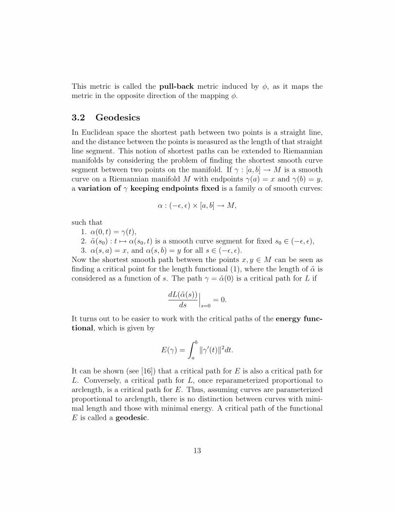
In Euclidean space the shortest path between two points is a straight line,and the distance between the points is measured as the length of that straightline segment. This notion of shortest paths can be extended to Riemannianmanifolds by considering the problem of finding the shortest smooth curvesegment between two points on the manifold. If γ : [a, b] → M is a smoothcurve on a Riemannian manifold M with endpoints γ(a) = x and γ(b) = y,a variation of γ keeping endpoints fixed is a family α of smooth curves:

α : (−ε, ε)× [a, b]→M,

such that1. α(0, t) = γ(t),2. α(s0) : t 7→ α(s0, t) is a smooth curve segment for fixed s0 ∈ (−ε, ε),3. α(s, a) = x, and α(s, b) = y for all s ∈ (−ε, ε).

Now the shortest smooth path between the points x, y ∈ M can be seen asfinding a critical point for the length functional (1), where the length of α isconsidered as a function of s. The path γ = α(0) is a critical path for L if

dL(α(s))

ds

∣∣∣s=0

= 0.

It turns out to be easier to work with the critical paths of the energy func-tional, which is given by

E(γ) =

∫ b

a

‖γ′(t)‖2dt.

It can be shown (see [16]) that a critical path for E is also a critical path forL. Conversely, a critical path for L, once reparameterized proportional toarclength, is a critical path for E. Thus, assuming curves are parameterizedproportional to arclength, there is no distinction between curves with mini-mal length and those with minimal energy. A critical path of the functionalE is called a geodesic.

13

Given a chart (x, U) a geodesic curve γ ⊂ U can be written in localcoordinates as γ(t) = (γ1(t), . . . , γn(t)). Using any such coordinate system,γ satisfies the following differential equation (see [16] for details):

d2γk

dt2= −

n∑i,j=1

Γkij(γ(t))dγi

dt

dγj

dt. (2)

The symbols Γkij are called the Christoffel symbols and are defined as

Γkij =1

2

n∑l=1

gkl(∂gjl∂xi

+∂gil∂xj− ∂gij∂xl

),

where gij denotes the entries of the inverse matrix g−1 of the Riemannianmetric.

Example 3.1. In Euclidean space Rn the Riemannian metric is given bythe identity matrix at each point p ∈ Rn. Since the metric is constant, theChristoffel symbols are zero. Therefore, the geodesic equation (2) reduces to

d2γk

dt2= 0.

The only solutions to this equation are straight lines, so geodesics in Rn mustbe straight lines.

Given two points on a Riemannian manifold, there is no guarantee that ageodesic exists between them. There may also be multiple geodesics connect-ing the two points, i.e., geodesics are not guaranteed to be unique. Moreover,a geodesic does not have to be a global minimum of the length functional, i.e.,there may exist geodesics of different lengths between the same two points.The next two examples demonstrate these issues.

Example 3.2. Consider the plane with the origin removed, R2 − {0}, withthe same metric as R2. Geodesics are still given by straight lines. There doesnot exist a geodesic between the two points (1, 0) and (−1, 0).

Example 3.3. Geodesics on the sphere S2 are given by great circles, i.e.,circles on the sphere with maximal diameter. This fact will be shown laterin the section on symmetric spaces. There are an infinite number of equal-length geodesics between the north and south poles, i.e., the meridians. Also,given any two points on S2 that are not antipodal, there is a unique greatcircle between them. This great circle is separated into two geodesic segmentsbetween the two points. One geodesic segment is longer than the other.

14

The idea of a global minimum of length leads to a definition of a distancemetric d : M ×M → R (not to be confused with the Riemannian metric). Itis defined as

d(p, q) = inf{L(γ) : γ a smooth curve between p and q}.

If there is a geodesic γ between the points p and q that realizes this dis-tance, i.e., if L(γ) = d(p, q), then γ is called a minimal geodesic. Minimalgeodesics are guaranteed to exist under certain conditions, as described bythe following definition and the Hopf-Rinow Theorem below.

Definition 3.2. A Riemannian manifold M is said to be complete if everygeodesic segment γ : [a, b]→M can be extended to a geodesic from all of Rto M .

The reason such manifolds are called “complete” is revealed in the nexttheorem.

Theorem 1 (Hopf-Rinow). If M is a complete, connected Riemannian man-ifold, then the distance metric d(·, ·) induced on M is complete. Furthermore,between any two points on M there exists a minimal geodesic.

Example 3.4. Both Euclidean space Rn and the sphere S2 are complete.A straight line in Rn can extend in both directions indefinitely. Also, agreat circle in S2 extends indefinitely in both directions (even though itwraps around itself). As guaranteed by the Hopf-Rinow Theorem, there isa minimal geodesic between any two points in Rn, i.e., the unique straightline segment between the points. Also, between any two points on the spherethere is a minimal geodesic, i.e., the shorter of the two great circle segmentsbetween the two points. Of course, for antipodal points on S2 the minimalgeodesic is not unique.

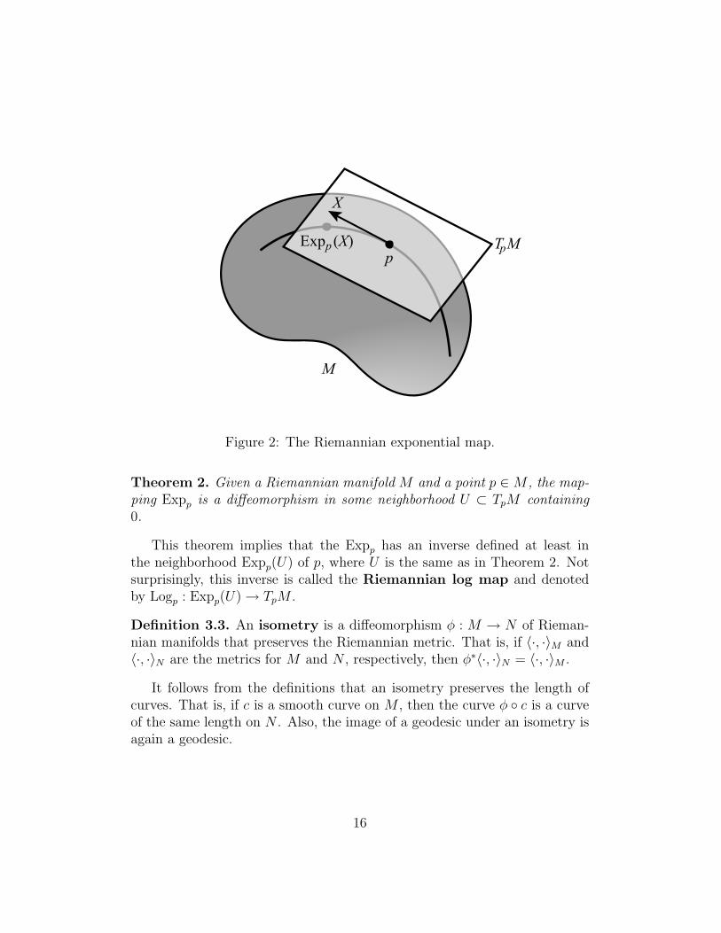
Given initial conditions γ(0) = p and γ′(0) = v, the theory of second-orderpartial differential equations guarantees the existence of a unique solutionto the defining equation for γ (2) at least locally. Thus, there is a uniquegeodesic γ with γ(0) = p and γ′(0) = v defined in some interval (−ε, ε). Whenthe geodesic γ exists in the interval [0, 1], the Riemannian exponentialmap at the point p (see Figure 2), denoted Expp : TpM →M , is defined as

Expp(v) = γ(1).

If M is a complete manifold, the exponential map is defined for all vectorsv ∈ TpM .

15

pT MpExp (X)p

X

M

Figure 2: The Riemannian exponential map.

Theorem 2. Given a Riemannian manifold M and a point p ∈M , the map-ping Expp is a diffeomorphism in some neighborhood U ⊂ TpM containing0.

This theorem implies that the Expp has an inverse defined at least inthe neighborhood Expp(U) of p, where U is the same as in Theorem 2. Notsurprisingly, this inverse is called the Riemannian log map and denotedby Logp : Expp(U)→ TpM .

Definition 3.3. An isometry is a diffeomorphism φ : M → N of Rieman-nian manifolds that preserves the Riemannian metric. That is, if 〈·, ·〉M and〈·, ·〉N are the metrics for M and N , respectively, then φ∗〈·, ·〉N = 〈·, ·〉M .

It follows from the definitions that an isometry preserves the length ofcurves. That is, if c is a smooth curve on M , then the curve φ ◦ c is a curveof the same length on N . Also, the image of a geodesic under an isometry isagain a geodesic.

16

4 Lie Groups

The set of all possible translations of Euclidean space Rn is again the spaceRn. A point p ∈ Rn is transformed by the vector v ∈ Rn by vector addition,p + v. This transformation has a unique inverse transformation, namely,translation by the negated vector, −v. The operation of translation is asmooth mapping of the space Rn. Composing two translations (i.e., additionin Rn) and inverting a translation (i.e., negation in Rn) are also smoothmappings. A set of transformations with these properties, i.e., a smoothmanifold with smooth group operations, is known as a Lie group. Manyother interesting transformations of Euclidean space are Lie groups, includingrotations, reflections, and magnifications. However, Lie groups also arisemore generally as smooth transformations of manifolds. This section is abrief introduction to Lie groups. More detailed treatments may be foundin [2, 4, 5, 6, 8, 16].

It is assumed that the reader knows the basics of group theory (see [7] foran introduction), but the definition of a group is listed here for reference.

Definition 4.1. A group is a set G with a binary operation, denoted hereby concatenation, such that

1. (xy)z = x(yz), for all x, y, z ∈ G,2. there is an identity, e ∈ G, satisfying xe = ex = x, for all x ∈ G,3. each x ∈ G has an inverse, x−1 ∈ G, satisfying xx−1 = x−1x = e.

As stated at the beginning of this section, a Lie group adds a smoothmanifold structure to a group.

Definition 4.2. A Lie group G is a smooth manifold that also forms agroup, where the two group operations,

(x, y) 7→ xy : G×G→ G Multiplication

x 7→ x−1 : G→ G Inverse

are smooth mappings of manifolds.

Example 4.1. The space of all n×n non-singular matrices forms a Lie groupcalled the general linear group, denoted GL(n). The group operation ismatrix multiplication, and GL(n) can be given a smooth manifold structureas an open subset of Rn2

. The equations for matrix multiplication and inverseare smooth operations in the entries of the matrices. Thus, GL(n) satisfies

17

the requirements of a Lie group in Definition 4.2. A matrix group is anyclosed subgroup of GL(n). Matrix groups inherit the smooth structure ofGL(n) as a subset of Rn2

and are thus also Lie groups. The books [3,5] focuson the theory of matrix groups.

Example 4.2. The n× n rotation matrices are a closed matrix subgroup ofGL(n) and thus form a Lie group. This group is called the special orthogo-nal group and is defined as SO(n) = {R ∈ GL(n) : RTR = I and det(R) =1}. This space is a closed and bounded subset of Rn2

, so it is compact bythe Heine-Borel theorem.

Given a point y in a Lie group G, it is possible to define the followingtwo diffeomorphisms:

Ly : x 7→ yx (Left multiplication)

Ry : x 7→ xy (Right multiplication)

A vector field X on a Lie group G is called left-invariant if it is invariantunder left multiplication, i.e., Ly∗X = X for every y ∈ G. Right-invariantvector fields are defined similarly. A left-invariant (or right-invariant) vectorfield is uniquely defined by its value on the tangent space at the identity,TeG.

Recall that vector fields on G can be seen as operators on the space ofsmooth functions, C∞(G). Thus two vector fields X and Y can be composedto form another operator XY on C∞(G). However, the operator XY is notnecessarily vector field. Surprisingly, however, the operator XY − Y X is avector field on G. This leads to a definition of the Lie bracket of vectorfields X, Y on G, defined as

[X, Y ] = XY − Y X. (3)

Definition 4.3. A Lie algebra is a vector space V equipped with a bilinearproduct [·, ·] : V × V → V , called a Lie bracket, that satisfies

(1) [X, Y ] = −[Y,X],(2) [[X, Y ], Z] + [[Y, Z], X] + [[Z,X], Y ] = 0,

for all X, Y, Z ∈ V.

The tangent space of a Lie group G, typically denoted g (a GermanFraktur font), forms a Lie algebra. The Lie bracket on g is induced by theLie bracket on the corresponding left-invariant vector fields. If X, Y are two

18

vectors in g, then let X, Y be the corresponding unique left-invariant vectorfields on G. Then the Lie bracket on g is given by

[X, Y ] = [X, Y ](e).

The Lie bracket provides a test for whether the Lie group G is commuta-tive. A Lie group G is commutative if and only if the Lie bracket on thecorresponding Lie algebra g is zero, i.e., [X, Y ] = 0 for all X, Y ∈ g.

Example 4.3. The Lie algebra for Euclidean space Rn is again Rn. The Liebracket is zero, i.e., [X, Y ] = 0 for all X, Y ∈ Rn. In fact, the Lie bracket forthe Lie algebra of any commutative Lie group is always zero.

Example 4.4. The Lie algebra for GL(n) is gl(n), the space of all real n×nmatrices. The Lie bracket operation for X, Y ∈ gl(n) is given by

[X, Y ] = XY − Y X.

Here the product XY denotes actual matrix multiplication, which turns outto be the same as composition of the vector field operators (compare to (3)).All Lie algebras corresponding to matrix groups are subalgebras of gl(n).

Example 4.5. The Lie algebra for the rotation group SO(n) is so(n), thespace of skew-symmetric matrices. A matrix A is skew-symmetric if A =−AT .

The following theorem will be important later.

Theorem 3. A direct product G1×· · ·×Gn of Lie groups is also a Lie group.

4.1 Lie Group Exponential and Log Maps

Definition 4.4. A mapping of Lie groups φ : G1 → G2 is called a Lie grouphomomorphism if it is a smooth mapping and a homomorphism of groups,i.e., φ(e1) = e2, where e1, e2 are the respective identity elements of G1, G2,and φ(gh) = φ(g)φ(h) for all g, h ∈ G1.

The image of a Lie group homomorphism h : R → G is called a one-parameter subgroup. A one-parameter subgroup is both a smooth curveand a subgroup of G. This does not mean, however, that any one-parametersubgroup is a Lie subgroup of G (it can fail to be an imbedded submanifoldof G, which is required to be a Lie subgroup of G). As the next theoremshows, there is a bijective correspondence between the Lie algebra and theone-parameter subgroups.

19

Theorem 4. Let g be the Lie algebra of a Lie group G. Given any vectorX ∈ g there is a unique Lie group homomorphism hX : R → G such thath′X(0) = X.

The Lie group exponential map, exp : g → G, not to be confusedwith the Riemannian exponential map, is defined by

exp(X) = hX(1).

Example 4.6. For the Lie group Rn the unique Lie group homomorphismhX : R→ Rn in Theorem 4 is given by hX(t) = tX. Therefore, one-parametersubgroups are given by straight lines at the origin. The Lie group exponentialmap is the identity. In this case the Lie group exponential map is the sameas the Riemannian exponential map at the origin. This is not always thecase, however, as will be shown later.

For matrix groups the Lie group exponential map of a matrix X ∈ gl(n)is computed by the formula

exp(X) =∞∑k=0

1

k!Xk. (4)

This series converges absolutely for all X ∈ gl(n).

Example 4.7. For the Lie group of 3D rotations, SO(3), the matrix ex-ponential map takes a simpler form. For a matrix X ∈ so(3) the followingidentity holds:

X3 = −θX, where θ =

√1

2tr(XTX).

Substituting this identity into the infinite series (4), the exponential map forso(3) can now be reduced to

exp(X) =

I, θ = 0,

I +sin θ

θX +

1− cos θ

θ2X2, θ ∈ (0, π).

The Lie group log map for a rotation matrix R ∈ SO(3) is given by

log(R) =

I, θ = 0,θ

2 sin θ(R−RT ), |θ| ∈ (0, π),

20

where tr(R) = 2 cos θ + 1.The exponential map for 3D rotations has an intuitive meaning. Any

vector X ∈ so(3), i.e., a skew-symmetric matrix, may be written in the form

X =

0 −z yz 0 −x−y x 0

.

If v = (x, y, z) ∈ R3, then the rotation matrix given by the exponential mapexp(X) is a 3D rotation by angle θ = ‖v‖ about the unit axis v/‖v‖.

21

References

[1] L. Auslander and R. E. MacKenzie. Introduction to Differentiable Man-ifolds. Dover, 1977.

[2] W. M. Boothby. An Introduction to Differentiable Manifolds and Rie-mannian Geometry. Academic Press, 2nd edition, 1986.

[3] M. L. Curtis. Matrix Groups. Springer-Verlag, 1984.

[4] J. J. Duistermaat and J. A. C. Kolk. Lie Groups. Springer, 2000.

[5] B. C. Hall. Lie groups, Lie algebras, and representations: an elementaryintroduction. Springer-Verlag, 2003.

[6] S. Helgason. Differential Geometry, Lie Groups, and Symmetric Spaces.Academic Press, 1978.

[7] I. N. Herstein. Topics in Algebra. John Wiley and Sons, 2nd edition,1975.

[8] K. Kawakubo. The Theory of Transformation Groups. Oxford Univer-sity Press, 1991.

[9] J. M. Lee. Riemannian Manifolds: An Introduction to Curvature.Springer, 1997.

[10] J. M. Lee. Introduction to Topological Manifolds. Springer, 2000.

[11] J. M. Lee. Introduction to Smooth Manifolds. Springer, 2002.

[12] J. W. Milnor. Morse Theory. Princeton University Press, 1963.

[13] J. W. Milnor. Topology from the Differentiable Viewpoint. PrincetonUniversity Press, 1997.

[14] J. R. Munkres. Topology: A First Course. Prentice-Hall, 1975.

[15] W. Rudin. Principles of Mathematical Analysis. McGraw-Hill, 1976.

[16] M. Spivak. A Comprehensive Introduction to Differential Geometry,volume 1. Publish or Perish, 3rd edition, 1999.

22

[17] M. Spivak. A Comprehensive Introduction to Differential Geometry,volume 2. Publish or Perish, 3rd edition, 1999.

[18] M. Spivak. A Comprehensive Introduction to Differential Geometry,volume 3. Publish or Perish, 3rd edition, 1999.

[19] M. Spivak. A Comprehensive Introduction to Differential Geometry,volume 4. Publish or Perish, 3rd edition, 1999.

[20] M. Spivak. A Comprehensive Introduction to Differential Geometry,volume 5. Publish or Perish, 3rd edition, 1999.

[21] L. A. Steen and J. A. Seebach. Counterexamples in Topology. Dover,1995.

23