Terrestrial mechanisms of interannual CO2 variability

Terrestrial mechanisms of interannual CO2 variability

N. ZengDepartment of Meteorology and Earth System Science Interdisciplinary Center, University of Maryland, College Park,Maryland, USA

A. Mariotti1

ENEA Climate Section, Rome, Italy

P. WetzelMax-Planck Institute for Meteorology, Hamburg, Germany

Received 30 March 2004; revised 19 November 2004; accepted 7 January 2005; published 2 March 2005.

[1] The interannual variability of atmospheric CO2 growth rate shows remarkablecorrelation with the El Nino Southern Oscillation (ENSO). Here we present results frommechanistically based terrestrial carbon cycle model VEgetation-Global-Atmosphere-Soil(VEGAS), forced by observed climate fields such as precipitation and temperature.Land is found to explain most of the interannual CO2 variability with a magnitude ofabout 5 PgC yr�1. The simulated land-atmosphere flux has a detrended correlation of0.53 (0.6 at the 2–7 year ENSO band) with the CO2 growth rate observed at MaunaLoa from 1965 to 2000. We also present the total ocean flux from the Hamburg OceanCarbon Cycle Model (HAMOCC) which shows ocean-atmosphere flux variation ofabout 1 PgC yr�1, and it is largely out of phase with land flux. On land, much of thechange comes from the tropical regions such as the Amazon and Indonesia where ENSOrelated climate anomalies are in the same direction across much of the tropics. Thesubcontinental variations over North America and Eurasia are comparable to the tropicsbut the total interannual variability is about 1 PgC yr�1 due to the cancellation fromthe subregions. This has implication for flux measurement network distribution. Thetropical dominance also results from a ‘‘conspiracy’’ between climate and plant/soilphysiology, as precipitation and temperature changes drive opposite changes innet primary production (NPP) and heterotrophic respiration (Rh), both contributing toland-atmosphere flux changes in the same direction. However, NPP contributes to aboutthree fourths of the total tropical interannual variation and the rest is fromheterotrophic respiration; thus precipitation appears to be a more important factor thantemperature on the interannual timescales as tropical wet and dry regimes controlvegetation growth. Fire, largely driven by drought, also contributes significantly to theinterannual CO2 variability at a rate of about 1 PgC yr�1, and it is not totally inphase with NPP or Rh. The robust variability in tropical fluxes agree well withatmospheric inverse modeling results. Even over North America and Eurasia, whereENSO teleconnection is less robust, the fluxes show general agreement with inversionresults, an encouraging sign for fruitful carbon data assimilation.

Citation: Zeng, N., A. Mariotti, and P. Wetzel (2005), Terrestrial mechanisms of interannual CO2 variability, Global Biogeochem.

Cycles, 19, GB1016, doi:10.1029/2004GB002273.

1. Introduction

[2] The observed atmospheric CO2 growth rate consistsof a large interannual variability superimposed on a gradual

increase due to human fossil fuel carbon release and landuse change (Figure 1) [Conway et al., 1994; Keeling et al.,1995; Houghton, 2000; Marland et al., 2001; Prentice etal., 2001]. In particular, the interannual CO2 variabilityshows a high correlation with the El Nino Southern Oscil-lation (ENSO). The CO2 growth rate measured at MaunaLoa has a correlation of 0.54 with the negative SouthernOscillation Index (SOI) at a lag of 5 months (Figure 2). Theinterannual variability amplitude is about 5 PgC yr�1. Such

GLOBAL BIOGEOCHEMICAL CYCLES, VOL. 19, GB1016, doi:10.1029/2004GB002273, 2005

1Also at Earth System Science Interdisciplinary Center, University ofMaryland, College Park, Maryland, USA.

Copyright 2005 by the American Geophysical Union.0886-6236/05/2004GB002273$12.00

GB1016 1 of 15

variability is a major source of uncertainty in our knowledgeof the ‘‘missing’’ carbon sink (about 2 PgC yr�1 [Dai andFung, 1993; Prentice et al., 2001]).[3] The interannual CO2 variability is mostly caused by

climate-driven variations in oceanic and terrestrial carbonsources and sinks because other factors such as fossil fuelemission and land use change on longer timescales. In orderto influence the carbon sources and sinks, ENSO anomalieshave to cascade through a host of processes, especially onland, such as land precipitation and temperature responsethrough teleconnection patterns, soil hydrology, and plantand soil physiology. Thus the high correlation between CO2

and ENSO is remarkable, as correlation often degradesdown the chain of causal links.[4] When the relation between CO2 and ENSO was first

noted [Bacastow, 1976], much of the focus was to explainthe CO2 variability based on oceanic changes. In particular,the equatorial Pacific Ocean has been identified as a majorregion of CO2 flux change. Although initially it was thoughtto have enhanced outgassing, it has now been shown toproduce up to 0.5 PgC yr�1 reduction in the outgassingduring El Nino years, largely due to the reduced upwellingof dissolved inorganic carbon from the cold waters below[Feely, 1987; Winguth et al., 1994; Francey et al., 1995;Feely et al., 2002]. Recent studies based on a variety ofmethods including pCO2 measurements, forward oceanmodeling, and atmospheric inversion found relatively mod-est oceanic contribution [Winguth et al., 1994; Ciais et al.,1995; Nakazawa et al., 1997; Lee et al., 1998; Feely et al.,2002; Le Quere et al., 2000, 2003; Bousquet et al., 2000;Roedenbeck et al., 2003; Wetzel et al., 2005].[5] In contrast to the general agreement on oceanic fluxes,

recent land carbon cycle research has produced widelydiffering results [e.g., Kaduk and Heimann, 1994; Knorr,2000; Prentice et al., 2000; Jones et al., 2001; McGuire etal., 2001; Dargaville et al., 2002; Schaefer et al., 2002] (seealso below). The degree to which these results explain the

amplitude and phasing of observed atmospheric CO2

changes varies greatly, and the exact partitioning betweenterrestrial and oceanic contributions remains uncertain. Forinstance, the interannual amplitude from four models ana-lyzed by Dargaville et al. [2002] differs by a factor of 2 to3, and the phasing also differs significantly compared toeach other or to inversion results. Even higher uncertaintiesexist when more detailed spatial patterns are consideredsuch as the relative contributions from the tropics versushigh latitudes, North America versus Eurasia, and monsoonregions versus subtropical savanna regions. Additional andimportant uncertainties come from anthropogenic processessuch as reforestation and nitrogen deposition which may

Figure 1. Anthropogenic CO2 emission and atmospheric CO2 growth rate (monthly from January 1965to June 2000 with seasonal cycle removed) at Mauna Loa, Hawaii, in PgC yr�1. Data are fromGLOBALVIEW-CO2 (2001). Also plotted below these is the negative Southern Oscillation Index (-SOI;in mbar) which is an indicator of the tropical ENSO phenomenon. See color version of this figure at backof this issue.

Figure 2. Lagged correlation between the observedCO2 growth rate and the negative Southern OscillationIndex (-SOI, solid circles), compared to the autocorrelationof SOI, for the period 1965–2000. CO2 at Mauna Loacorrelates with -SOI at 0.54 at about 5 months lag.

GB1016 ZENG ET AL.: INTERANNUAL CO2 VARIABILITY

2 of 15

GB1016

interfere with ‘‘natural’’ interannual variability which wouldbe occurring in their absence.[6] The physical and biological mechanisms of such

changes are not very well known. Some terrestrial carbonmodeling and data analysis has suggested that ENSO relatedtemperature variation is a dominant factor [Kindermann etal., 1996; Braswell et al., 1997; Gerard et al., 1999], but thestrength of respiration and soil decomposition rate depen-dence on temperature is highly uncertain on global scalesand is model dependent [Trumbore et al., 1996; Liski et al.,1999; Kirschbaum, 2000;Giardina and Ryan, 2000; Barrett,2002; Melillo et al., 2002]. Thus this sensitivity dependslargely on a parameterization not very well constrained.Others found a major contribution from precipitation throughits impact on soil moisture and subsequently NPP [Craig,1998; Tian et al., 1998; Foley et al., 2002; Nemani et al.,2003], while yet others foundmore comparable contributionsor more complicated regional dependence [Jones et al., 2001;

Cao and Prince, 2002]. A less studied factor is change insolar radiation which could also play an important role, suchas during the post-Pinatubo period 1991–1993 [Knorr, 2000;Roderick et al., 2001; Gu et al., 2003; Reichenau and Esser,2003] and possibly on decadal timescales [Nemani et al.,2003], but its relative importance and pathway have been amatter of controversy [Angert et al., 2004]. Firemay also playan important role because drought induced by climateanomalies is a major driver of fire occurrence [Keeling etal., 1995; Page et al., 2002; Langenfelds et al., 2002; van derWerf et al., 2004], which may be further enhanced by humaninterventions, as man-made fires tend to happen under dryconditions.[7] Here we use a terrestrial carbon cycle model forced by

observed climate variability to study the mechanisms un-derlying the interannual atmospheric CO2 variability, focus-ing on the spatial and temporal patterns of the variation incarbon sources and sinks, and how physical climate anoma-

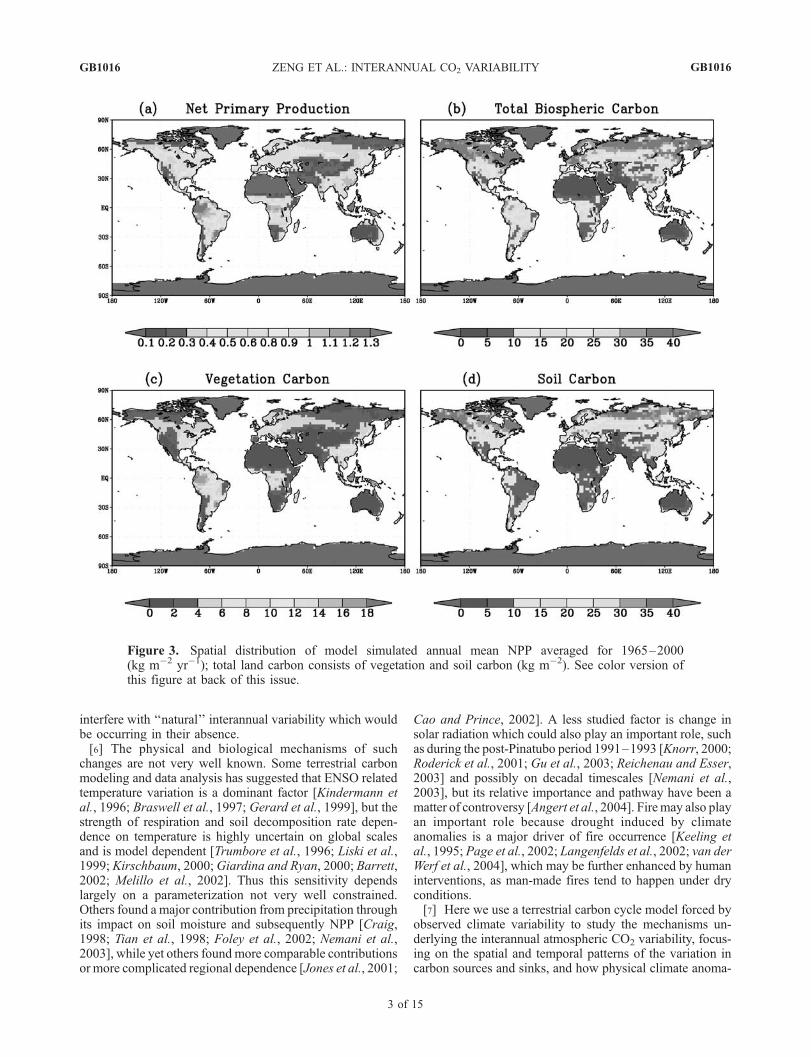
Figure 3. Spatial distribution of model simulated annual mean NPP averaged for 1965–2000(kg m�2 yr�1); total land carbon consists of vegetation and soil carbon (kg m�2). See color version ofthis figure at back of this issue.


3 of 15

GB1016

lies interact with biochemistry to produce the observedchanges. We also present a glimpse of total ocean flux froman ocean carbon model with the details discussed by Wetzelet al. [2005]. Our analysis focuses on land as it is the majorsource of interannual variability as well as the larger sourceof uncertainty.

2. Methodology

[8] The terrestrial carbon model VEgetation-Global-Atmosphere-Soil (VEGAS) [Zeng, 2003] (see alsoAppendix A) is coupled to the physical land surfacemodel Simple-Land (SLand [Zeng et al., 2000a]). The landmodel was forced by the observed land precipitation andtemperature ofNew et al. [2000], updated by T. D.Mitchell etal. (A comprehensive set of high-resolution grids of monthlyclimate for Europe and the globe: The observed record(1901–2000) and 16 scenarios (2001–2100), submitted toJournal of Climate, 2004) to cover the period of 1901–2000.The seasonal climatologies of radiation, humidity, and windspeed are used so that the potential CO2 variability related tothese, in particular, the change in radiation, is not studied here.Atmospheric CO2 for photosynthesis was held at constantpreindustrial value, as the greenhouse effect variation oninterannual timescale is very small. The Hamburg OceanCarbon Cycle Model (HAMOCC [Six and Maier-Reimer,1996] (see also results from the most recent version 5 ofWetzel et al. [2005]) was forced by a physical ocean modelwhich is in turn forced by the near-surface atmospheric fieldsfrom the NCEP/NCAR reanalysis [Kalnay et al., 1996]. Thisindirect approach may lead to some uncertainties as thephysical model may not best represent the actual oceanvariabilities.[9] The land model was run at 2.5� � 2.5� resolution

using 1901 climate forcing repeatedly until the carbon poolsreach equilibrium with the climate. This state was then usedas the initial condition for the 1901–2000 run. Figure 3shows the annual mean fields averaged for 1965–2000 ofNPP, total land, vegetation, and soil carbon pools. WhileNPP follows closely precipitation in the tropics, temperatureand radiation are also important for high-latitude produc-tivity. The simulated NPP is similar to the average of model

results from the Potsdam NPP Model Intercomparisonproject [Cramer et al., 1999] both in terms of the spatialpattern and range. Vegetation carbon is high in the tropicaland midlatitude moist regions, but soil carbon poolsare dominated by higher-latitude cold regions becauseof the slow soil decomposition rate there. The globaltotal gross primary production (GPP) is 122 PgC yr�1,NPP is 58 PgC yr�1, vegetation carbon pool is 550 PgC,and soil carbon is 1850 PgC, within the range of observa-tionally based estimates.[10] Most of the analysis here focuses on the period

1965–2000 when noninterrupted CO2 observations fromMauna Loa are available (Figure 1), and the seasonal cycleshave been removed by a 12-month running mean filterbecause the focus here is the interannual variability. Ideally,the surface-atmosphere flux should be compared withglobal total CO2 growth rate, but only the Mauna LoaCO2 time series spans several decades, and it has beenshown that the Mauna Loa data can be used as a proxy ofglobal CO2, especially on interannual and longer timescaleswhich are substantially longer than CO2 mixing time in theatmosphere [Gammon et al., 1985]. The slight trend in theCO2 data is mostly due to the increasing anthropogenicemission (Figure 1), and it does not have a major impact onthe interannual focus here.

3. Global Total and Spatial Patterns

[11] Figure 4 shows the model simulated global total landto atmosphere carbon flux. The range of interannual varia-tions is from �6 to 2 PgC yr�1. In particular, land was alarge carbon source of 2 PgC yr�1 to the atmosphere duringthe 1997–1998 El Nino event, followed by a 2.5 PgC yr�1

sink during the ensuing La Nina event. Overall, the modelland-atmosphere flux agrees well with the CO2 growth rateobserved at Mauna Loa both in terms of interannualamplitude and phasing, with a correlation of 0.53 after thetrends are removed. The correlation is higher at 0.6 onENSO timescales after a band-pass filter of 2–7 years isapplied to the data. This is because the correlation ondecadal timescale is significantly lower, so that after re-moving the lower frequencies, the interannual correlation

Figure 4. Monthly carbon flux from land to the atmosphere from January 1965 to June 2000 (labeled onthe left in PgC yr�1), simulated using the terrestrial carbon model VEGAS forced by the observedprecipitation and temperature, compared to CO2 growth rate observed at Mauna Loa, Hawaii (labeled onthe right). Seasonal cycle has been removed from both using 12-month running mean. The observed CO2

growth rate has higher values because it also contains the anthropogenic emission signal, and note thedifferent scale for CO2 growth rate on the right. The correlation between the two is 0.53 after removingthe trends. See color version of this figure at back of this issue.


4 of 15

GB1016

becomes higher. We also compared the model flux withtotal land-atmosphere flux from the inversion of Bousquet etal. [2000] for 1980–1998, and the result is very similar tothe comparison with Mauna Loa CO2 growth here. The fastsubseasonal variations in the CO2 growth rate are likely dueto influence of synoptic atmospheric circulation at a singlemeasuring station. The modeled land-atmosphere flux has acorrelation of 0.58 with the negative SOI index at 3 monthslag.[12] Most noticeable differences are 1991–1993, 1969–

1970, and to a lesser extent, 1982–1983. The discrepanciesduring 1991–1993 and 1982–1983 have been attributed tovolcanic aerosol effects, but the issue is still a matter ofdebate [Jones and Cox, 2001; Lucht et al., 2002; Gu et al.,2003; Krakauer and Randerson, 2003; Angert et al., 2004].In particular, Jones and Cox [2001] and Lucht et al. [2002]were able to explain part of the unusual flux anomaliesduring the 1991–1993 and 1982–1983 periods using thecooling caused by Pinatubo and El Chichon volcanicaerosols. Our model does not reproduce the full amplitudeand phasing of these changes, despite the fact that thevolcanic cooling is included in the temperature forcing data.One source of difference is that Jones and Cox used acoupled carbon-climate model which produced regionalclimate anomalies somewhat different from the observationsused in our model (despite the general agreement globally),while Lucht et al. studied only the contribution from theboreal regions. Our results here are compared to observa-tions in greater details.[13] If precipitation and temperature change cannot ex-

plain the early CO2 drawdown during the Pinatubo periodas our model results suggest, one is forced to turn to othermechanisms. One such possibility is enhanced diffuse lightdue to the large volcanic aerosol loading [Roderick et al.,2001; Gu et al., 2003]. However, the degree to which thiscan explain the CO2 change is not clear [Angert et al.,2004], and tree ring study does not appear to supportenhanced growth after historical volcanic eruptions[Krakauer and Randerson, 2003].[14] While this work focuses on terrestrial sources and

sinks, ocean also plays a nonnegligible role. In order to put

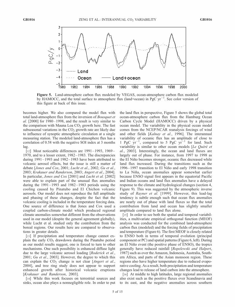
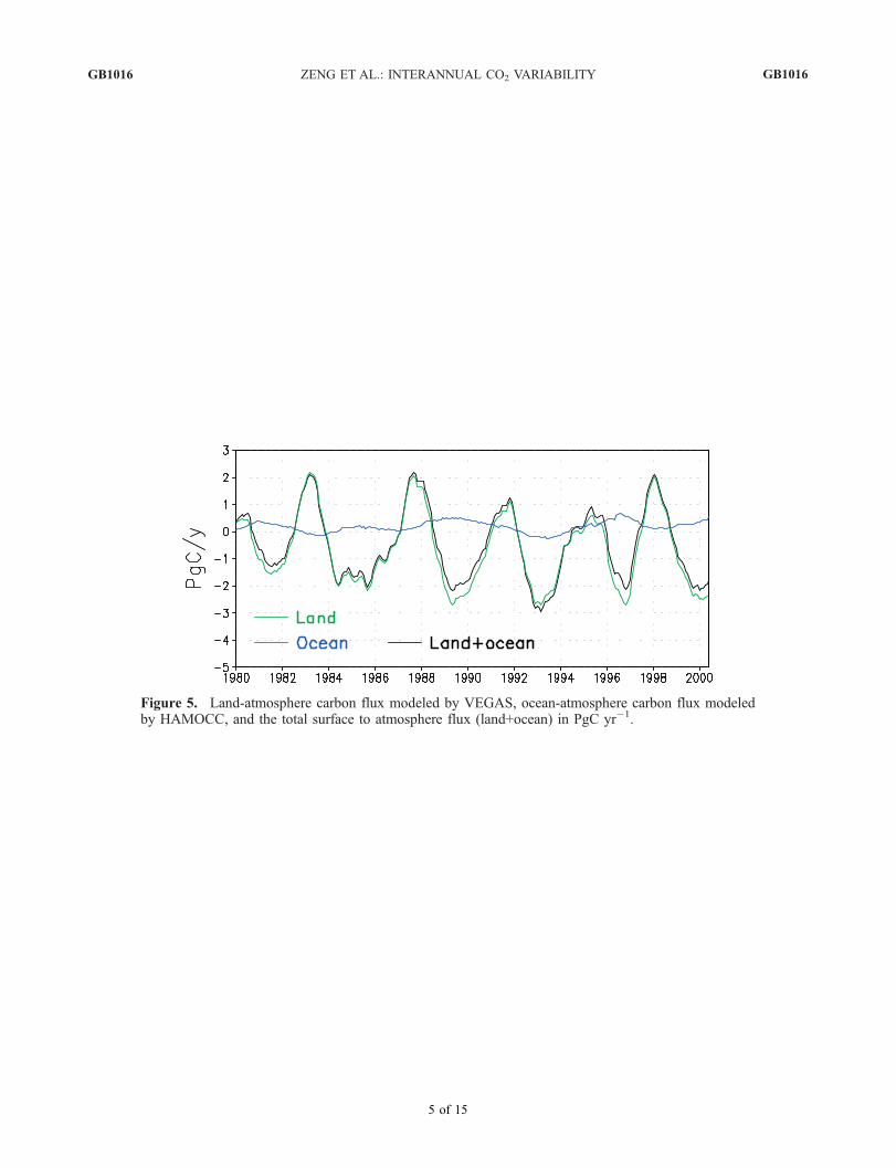
the land flux in perspective, Figure 5 shows the global totalocean-atmosphere carbon flux from the Hamburg OceanCarbon Cycle Model (HAMOCC) driven by a physicalocean model. The variability in the physical ocean modelcomes from the NCEP/NCAR reanalysis forcings of windand other fields [Kalnay et al., 1996]. The interannualvariability of oceanic flux has an amplitude of close to1 PgC yr�1, compared to 5 PgC yr�1 for land. Suchvariability is similar to other ocean models [Le Quere etal., 2003]. Interestingly, the ocean and land fluxes arelargely out of phase. For instance, from 1997 to 1998 asthe El Nino becomes stronger, oceanic flux decreased whileland flux increased. During the transitions such as the1996–1997 transition to El Nino and early 1998 transitionto La Nina, ocean anomalies appear somewhat earlierbecause ENSO signal first appears in the equatorial Pacificand Indian oceans and land flux anomalies have a delayedresponse to the climate and hydrological changes (section 4,Figure 9). This was suggested by the atmospheric inversestudy of Rayner et al. [1999]. However, this lead-lagtendency is subtle enough such that ocean flux anomaliesare nearly out of phase with land fluxes so that the totalcontribution from land and ocean has slightly smalleramplitude compared to land flux alone.[15] In order to see both the spatial and temporal variabil-

ities, a multivariate empirical orthogonal function (MEOF)analysis was conducted for the combined land-atmospherecarbon flux (modeled) and the forcing fields of precipitationand temperature (Figure 6). The first MEOF is closely relatedto ENSO both in terms of temporal evolution (principalcomponent or PC) and spatial patterns (Figure 6, left). Duringan El Nino event (the positive phase of ENSO), the tropicsgenerally have reduced rainfall [Ropelewski and Halpert,1987] such as over the Amazon, Indonesia, Australia, South-ern Africa, and parts of the Asian monsoon region. Theseregions also have higher temperature due to reduced evapo-rative cooling. As a result, both precipitation and temperaturechanges lead to release of land carbon into the atmosphere.[16] At middle to high latitudes, large regional anomalies

also exist such as the positive fluxes over Scandinavia andto its east, and the negative anomalies across southern

Figure 5. Land-atmosphere carbon flux modeled by VEGAS, ocean-atmosphere carbon flux modeledby HAMOCC, and the total surface to atmosphere flux (land+ocean) in PgC yr�1. See color version ofthis figure at back of this issue.


5 of 15

GB1016

Figure 6. Time evolution (principal components or PC) and spatial patterns of the first two MEOF froma detrended multivariate empirical orthogonal function (MEOF) analysis of modeled land-atmospherecarbon flux, observed precipitation, and temperature. Plotted together with PC1 is the SouthernOscillation Index (SOI, green line). The spatial patterns of MEOF1 of precipitation and temperature areENSO-like, while MEOF2 temperature is similar to multidecadal surface warming pattern. See colorversion of this figure at back of this issue.


6 of 15

GB1016

Europe and central Asia. At these latitudes, precipitationand temperature have a less straightforward relation than inthe tropics. In North America, large spatial variations occurfrom northwestern to southeastern United States as well asfrom Alaska to Canada. When summed over a continentsuch as North America, the subcontinental variations tend tocancel each other so that the total contribution from thecontinent is small compared to tropical regions. Furtherdetails of these mechanisms are discussed in section 4.[17] The El Nino event in 1997–1998 was the largest in

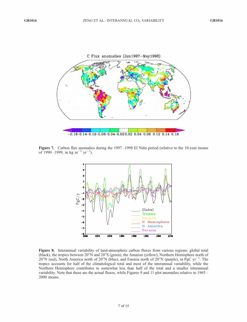
the twentieth century; Figure 7 shows a tropical-widerelease of carbon into the atmosphere such as over theAmazon, Indonesia, and Eastern Australia. In the extra-tropics, major sinks are located along the east and westcoasts of North America and the southern Europe and BlackSea region, while many other regions are mild sources.[18] It is interesting to compare this particular event with

the MEOF1 pattern in Figure 6 which depicts long-termspatially coherent variability dominated by ENSO. Thetropical patterns such as over South America are largelysimilar, with notable exception in southern Africa where1997–1998 has a negative anomaly while the MEOF1pattern shows strong positive flux. Extratropics showslarger differences especially over North America, but thesink anomalies over southern Europe–central Asia and thetripole pattern over East Asia appear to be more consistent.Thus, farther away from the tropics, the teleconnection ofENSO influence becomes weaker, and the response incarbon cycle also becomes less robust.[19] The second MEOF (Figure 6, right) depicts multi-

decadal variation that is largely a signature of the twentiethcentury global temperature change. This linkage can be seenin the warming of the 1940s, cooling in the 1960s andsubsequent warming since the 1970s [Hansen et al., 1996;Stott et al., 2000]. An overall warming caused tropical and

midlatitude carbon release as plant respiration and soildecomposition increase. Interestingly, the strong warmingat high latitude, especially over Siberia, leads to a carbonsink due to enhanced vegetation growth because these cold

Figure 7. Carbon flux anomalies during the 1997–1998 El Nino period (relative to the 10-year meansof 1990–1999, in kg m�2 yr�1). See color version of this figure at back of this issue.

Figure 8. Interannual variability of land-atmospherecarbon fluxes from various regions: global total (black),the tropics between 20�N and 20�S (green), the Amazon(yellow), Northern Hemisphere north of 20�N (red), NorthAmerica north of 20�N (blue), and Eurasia north of 20�N(purple), in PgC yr�1. The tropics accounts for half of theclimatological total and most of the interannual variability,while the Northern Hemisphere contributes to somewhatless than half of the total and a smaller interannualvariability. Note that these are the actual fluxes, whileFigures 9 and 11 plot anomalies relative to 1965–2000means. See color version of this figure at back of this issue.


7 of 15

GB1016

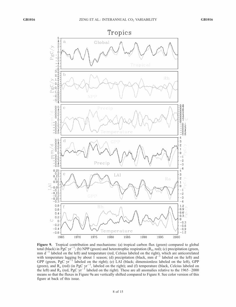
Figure 9. Tropical contribution and mechanisms: (a) tropical carbon flux (green) compared to globaltotal (black) in PgC yr�1; (b) NPP (green) and heterotrophic respiration (Rh, red); (c) precipitation (green,mm d�1 labeled on the left) and temperature (red, Celsius labeled on the right), which are anticorrelatedwith temperature lagging by about 1 season; (d) precipitation (black, mm d�1 labeled on the left) andGPP (green, PgC yr�1 labeled on the right); (e) LAI (black; dimensionless labeled on the left), GPP(green), and Ra (red) (in PgC yr�1, labeled on the right); and (f) temperature (black, Celcius labeled onthe left) and Rh (red, PgC yr�1 labeled on the right). These are all anomalies relative to the 1965–2000means so that the fluxes in Figure 9a are vertically shifted compared to Figure 8. See color version of thisfigure at back of this issue.


8 of 15

GB1016

regions are strongly temperature limited [Zhou et al., 2001;Lucht et al., 2002]. Precipitation of MEOF2 also appearsimportant in various regions, such as over the Europe-Mediterranean-central Asian region where a North AtlanticOscillation (NAO) related pattern [Mariotti et al., 2002] ispartly responsible for the positive carbon flux.[20] An implication of these results is that the variability

of carbon sources and sinks has multiple spatial andtemporal scales. Because the spatial variations are typicallysubcontinental, atmospheric inversions with continentalresolution return aggregated results due to cancellation ofdifferent regions. On the other hand, these spatial patternsare coherent and large scale, reflecting the characteristicclimate anomaly patterns; thus subcontinental observationalnetwork such as the FLUXNET, if reasonably distributed,will be able to capture much of these climate relatedchanges in carbon sources and sinks.

4. Regional Contributions

[21] Figure 8 shows the global total land to atmosphereflux and the contributions from a few selected regions: thewhole tropics from 20�S to 20�N, the Amazon, Northern

Hemisphere extratropics (north of 20�N), North America,and Eurasia. The land-atmosphere flux is dominated bycontribution from the tropics with an interannual amplitudeof about 5 PgC yr�1. The Amazon region alone contributesabout half of the total tropical flux (more than 2 PgC yr�1).The Amazon thus contributes a disproportionately largefraction to the total flux (its total area is less than one thirdof the tropical land). The Northern Hemisphere extratropicsconsists of North America and Eurasia, it contributes asmall fraction of the total variability, and it has only a weakcorrelation with the total flux which follows ENSO closely.We now take a closer look at the processes responsible forthese changes.

4.1. Tropics

[22] The dominance of the tropics can be seen clearly inFigure 9a as most of the global total land-atmospherecarbon flux can be explained by the tropical contribution.To understand the origin of this tropical contribution, totalland to atmosphere flux Fta is split into net primaryproduction (NPP: gross primary production GPP minusplant respiration Ra) and heterotrophic respiration (Rh: soilto atmosphere flux),

Fta ¼ Rh � NPP: ð1Þ

Fta is sometimes referred to as net carbon exchange (NCE)or net biome exchange (NBE), and we do not consider thecontribution from anthropogenic effects in our model. Ingeneral, NPP and Rh vary in the opposite direction such thatthey contribute to Fta in the same direction (Figure 9b).However, the amplitude of Rh is smaller than NPP. Forinstance, from the 1997–1998 El Nino to 1999–2000 LaNina, NPP increased by 4 PgC yr�1 while Rh dropped by1.7 PgC yr�1. Thus Rh contributes to less than one third ofthe total Fta change while NPP contributes the remainder.[23] The change in NPP and Rh can be understood using

Figures 9c–9f. Leaf area index (LAI) (Figure 9e), anindicator of leaf biomass, correlates closely with GPP withslight lag because part of the assimilated carbon throughGPP is converted into leaf biomass almost immediately.Autotrophic respiration Ra (vegetation to atmosphere car-bon flux) follows GPP and LAI with a lag of a few monthsas the vegetation carbon anomalies gets respired.[24] The change in GPP follows precipitation (Figure 9d)

closely with a lag of about one season because soil moistureresponds to precipitation with a delay [Zeng, 1999] whichdetermines the photosynthesis rate. Soil respiration Rh

correlates very well with temperature (Figure 9f). Interest-ingly, Rh appears to lead rather than lag temperature (albeitonly slightly), which could be due to factors other thantemperature such as soil decomposition rate dependence onsoil moisture which may lead temperature because precip-itation leads temperature (Figure 9c). Alternatively, anincreased turnover from litterfall in response to early pre-cipitation and growth can also lead to an early increase inrespiration [Gu et al., 2004].[25] The fact that precipitation and temperature are anti-

correlated (Figure 9c) is not a coincidence and has funda-mental importance for the tropical flux. In the tropics where

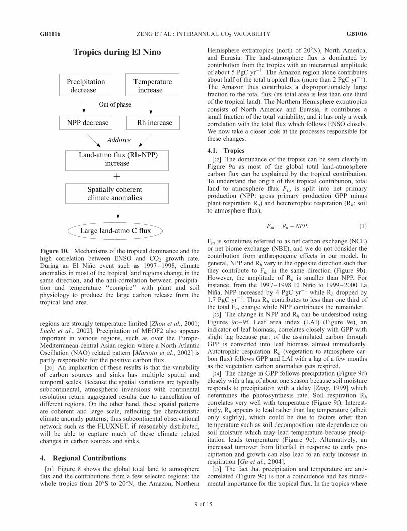
Tropics during El Nino

Figure 10. Mechanisms of the tropical dominance and thehigh correlation between ENSO and CO2 growth rate.During an El Nino event such as 1997–1998, climateanomalies in most of the tropical land regions change in thesame direction, and the anti-correlation between precipita-tion and temperature ‘‘conspire’’ with plant and soilphysiology to produce the large carbon release from thetropical land area.


9 of 15

GB1016

Figure 11. Northern Hemisphere land contribution and mechanisms: (a) Northern Hemisphereextratropics (north of 20�N) flux anomalies (green) compared to global total (black) in PgC yr�1;(b) NPP (green) and heterotrophic respiration (red); and (c) Precipitation (green, mm d�1 labeled on the left)and temperature (red, Celsius labeled on the right). The correlation between precipitation and temperaturegives rise to largely covarying NPP and Rh which partially cancel each other, leading to a relatively smallcontribution to the global total carbon flux. See color version of this figure at back of this issue.

Figure 12. Model carbon fluxes (PgC yr�1) from North America and Eurasia from 1987 to 1998compared to those from the atmospheric inversion of Bousquet et al. [2000]. See color version of thisfigure at back of this issue.


10 of 15

GB1016

thermodynamics and the hydrological cycle dominatessurface energy balance, a decrease in precipitation leads todrier land surface and less evapotranspiration, thus lessevaporative cooling and higher temperature, and vice versa[Zeng and Neelin, 1999]. During El Nino, this thermody-namic effect tends to outweigh the direct tropical warmingdue to atmospheric dynamics which is nonetheless in thesame direction. On one hand, decreased precipitation duringan El Nino leads to lower soil moisture, and thus lower GPPand NPP (less carbon uptake); on the other hand, warmertemperature leads to more respiration carbon loss, bothleading to carbon loss to the atmosphere. Thus the anti-correlation between precipitation and temperature ‘‘con-spire’’ with plant and soil physiology to produce the largecarbon release from the tropical land area during an El Ninoevent. This is further enhanced by the fact that during suchan event, most of the tropical land has reduced rainfall suchas over the Amazon, Indonesia, eastern Australia, andsouthern Africa (Figure 6); thus they all contribute toincreased atmospheric CO2 during an El Nino. Thesemechanisms are further illustrated in Figure 10. In contrast,higher latitudes behave differently in many of these aspects,to which we shift our attention now.

4.2. Northern Hemisphere Extratropics

[26] The contribution from the Northern Hemisphereextratropics (north of 20�N; Figure 11a) is relatively smallcompared to the total land-atmosphere carbon flux which isdominated by the tropics. The temporal variation also showssomewhat less coherent ENSO signal, but nonethelesslargely changes in the same direction as the tropics with adelay of a few months. The Northern Hemisphere contri-bution is small despite the large land area because of acancellation from different subcontinental regions as dis-cussed in section 3 (Figure 6). Second, at middle to highlatitudes where precipitation is mostly in the form of large-scale condensation as a result of dynamic baroclinic insta-bility, high temperature leads to high relative humidity and

often more rainfall [Zeng et al., 2000b]. This positivecorrelation in precipitation and temperature (Figure 11c),together with their respective influence on plant growth andrespiration, leads to positive correlation between NPP andRh (Figure 11b); thus they partially compensate each other(equation (1)). As a result of these largely compensatingfactors, higher latitude contribution to interannual CO2

variability as a whole is significantly smaller than thetropics, despite that the anomalies may be large on subcon-tinental scales (Figure 6). Interestingly, unlike in the tropicswhere Rh is much smaller than NPP, at high latitudes theyhave comparable sizes.[27] The Northern Hemisphere extratropics consists of

North America and Eurasia. The interannual amplitude isabout 1 PgC y�1 for both regions (Figure 12). Thesevariabilities compare favorably with the inverse modelingresults from 1988 to 1998 [Bousquet et al., 2000], but theinverse modeling shows somewhat larger amplitude inNorth America. They also show general agreement withthe inversion of Roedenbeck et al. [2003, Figure 5], al-though similarly large differences also exist between thetwo inversions, especially over Eurasia. The convergencebetween the forward modeling approach and inverse modelresults in these regions with relatively weak ENSO signalsuggesting a certain confidence in the results. Such conver-gence also lends optimism to carbon data assimilation.

5. Contribution From Fire

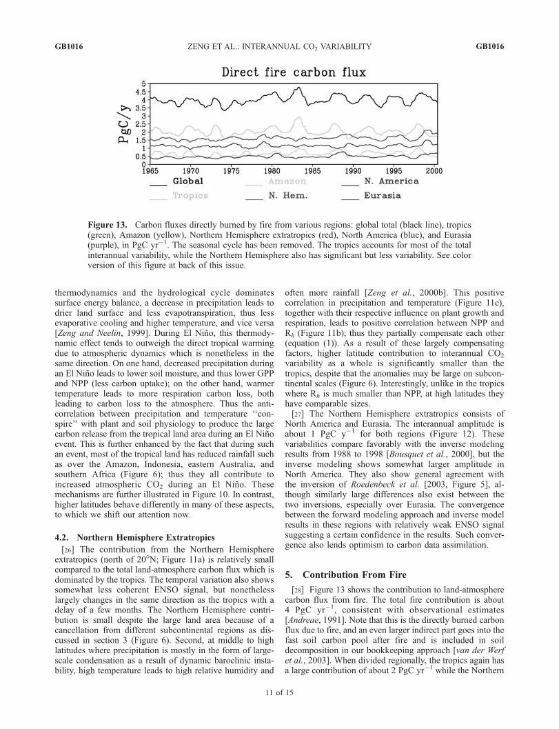
[28] Figure 13 shows the contribution to land-atmospherecarbon flux from fire. The total fire contribution is about4 PgC yr�1, consistent with observational estimates[Andreae, 1991]. Note that this is the directly burned carbonflux due to fire, and an even larger indirect part goes into thefast soil carbon pool after fire and is included in soildecomposition in our bookkeeping approach [van der Werfet al., 2003]. When divided regionally, the tropics again hasa large contribution of about 2 PgC yr�1 while the Northern

Figure 13. Carbon fluxes directly burned by fire from various regions: global total (black line), tropics(green), Amazon (yellow), Northern Hemisphere extratropics (red), North America (blue), and Eurasia(purple), in PgC yr�1. The seasonal cycle has been removed. The tropics accounts for most of the totalinterannual variability, while the Northern Hemisphere also has significant but less variability. See colorversion of this figure at back of this issue.


11 of 15

GB1016

Hemisphere contributes about 1.5 PgC yr�1, with theremainder from the Southern Hemisphere.[29] The amplitude of interannual fire carbon flux

variability is about 1 PgC yr�1, or about 20% of thetotal land-atmosphere flux anomaly. This also comesmostly from the tropics, where large wet and dryepisodes control the soil wetness and fire regimes. Ofthe tropical contribution, the Amazon basin aloneaccounts for 30% to 40% of the climatological andinterannual values. The variation in the Northern Hemi-sphere does not show a simple correlation with thetropical signal, with an interannual amplitude of about0.5 PgC yr�1. However, during 1997–1999, NorthernHemisphere appears to have equally large fire flux withmore than 1 year lag from the tropical flux.[30] A question of considerable interest is how important

carbon flux variability is relative to normal heterotrophicrespiration. Figure 14 shows the interannual anomalies inglobal total Rh, Ra, and fire carbon flux CFire. In ourbookkeeping approach, the burned aboveground biomass(live leaf+wood) is lumped into Ra, while the burned fastsoil carbon (mostly litterfall) is lumped into Rh, with theaboveground contribution dominant. The interannual vari-ability of fire flux can be as large as 1 PgC yr�1, about halfof the Rh or Ra. While Rh and Ra tend to covary due to thecommon influence from temperature, fire flux is often not inphase. Thus although fire contribution can be highly sig-nificant, especially compared to the Ra, the larger part of Rh

and Ra variabilities still come from normal respiration.Obviously this is an aspect sensitive to model parameteri-zation and needs to be further studied.[31] Thus our simulated fire flux is less than the estimate of

Page et al. [2002], who found a contribution of 0.81 to2.57 PgC yr�1 from Indonesia in 1997 alone, while ourtropical total fire flux is about 2 PgC yr�1 and 2.5 PgC yr�1

during 1997–1998 with major contribution from the Ama-zon.However, human drained peatland firewas amajor factorin their study, while our model does not include anthropo-genic effect. Our amplitude is also less than the estimate ofvan derWerf et al. [2004] where fire contribution accounts forabout 65% of the total flux anomaly during 1997–1998 ElNino, while ours is about 20%. Since van der Werf et al. usedsatellite observations of fire counts while we consideredclimate variability only, we may have again missed possiblehuman-induced fire contribution which could enhance natu-ral anomalies. However, the different methods and models

usedmay still be themajor reason for the differences, asmanyprocesses such as the estimate of fuel load and burned area arestill poorly constrained.[32] Our result is more in line with Langenfelds et al.

[2002], who estimated 0.8–3.7 PgC additional (relative tonormal year) fire C flux for the 1997/1998 El Nino period,while our model predicts about 1 PgC. Apart from uncertain-ties in model parameterization, our model does not consideranthropogenic impact on fire which tends to enhance fireextremes. The large range in their estimate is on one hand dueto the difficulty in distinguishing flux contribution of theimbalance in photosynthesis and respiration from that of fire,and on the other hand due to the uncertain CH4/CO2 or H2/CO2 ratios from biomass burning.

6. Conclusions

[33] The high-precision atmospheric CO2 measurementsat Mauna Loa and other places indicate large interannualvariability of CO2 growth rate on the order of 5 PgC yr�1

that can be attributed to terrestrial and oceanic sources andsinks. We have used terrestrial and ocean carbon cyclemodels forced by observed climate variability to study themechanisms underlying the interannual atmospheric CO2

variability.[34] In agreement with some recent studies, we found that

most of the interannual variability in the observed CO2

growth rate can be explained by climate forced changes inthe terrestrial biosphere with an interannual amplitude of 4–5 PgC yr�1. Ocean-atmosphere flux has an interannualvariability of 1 PgC yr�1, and it is largely out of phasewith terrestrial flux.[35] Most of the land-atmosphere flux variability comes

from the tropics where ENSO related climate anomaliesimpact the hydrological cycle and energy balance in acoherent fashion. The tropical dominance and high correla-tion with ENSO can be attributed to two major factors usingEl Nino warm event as example with La Nina largelyopposite sign:[36] 1. The first factor is the spatial coherence of climate

anomalies. During an El Nino event, most of the tropicsexperiences reduction of rainfall and higher temperature asthe result of shifting atmospheric circulation, such as overthe Amazon, Indonesia, southeastern Asia, eastern Aus-tralia, and Africa. These coherent changes lead to carbonrelease from all these regions.

Figure 14. Anomalies of global carbon fluxes relative to 1980–2000 mean due to heterotrophicrespiration (Rh), autotrophic respiration (Ra), and direct fire (Cfire), in PgC yr�1. See color version of thisfigure at back of this issue.


12 of 15

GB1016

[37] 2. The second factor is a ‘‘conspiracy’’ betweenclimate anomalies and plant/soil physiology. A reductionin tropical rainfall leads to higher temperature due to lessevaporative cooling; then reduced moisture lowers plantproductivity NPP (less carbon uptake), and higher temper-ature increases heterotrophic respiration Rh (more carbonrelease), thus leading to additive carbon release to theatmosphere.[38] In both respects, extratropics behave differently: The

large subcontinental spatial variations lead to cancellationfrom different regions, and the positive correlation betweenprecipitation and temperature there gives rise to additionalcancellation from positively correlated NPP and Rh. Anadditional factor is that at high-latitude temperature-limitedregions, higher temperature means more growth which addsto the complexity in extratropics, but the overall effects ofall these still lead to large cancellations.[39] Of the contributions from NPP and Rh in the tropics,

NPP contributes to about three fourths of the total flux inresponse to change in precipitation, thus supporting thenotion that precipitation has a larger effect than temperatureas NPP mostly responds to precipitation and Rh respondsmostly to temperature. This is partly because tropical andsubtropical regions are dominated by wet and dry climateregimes which control plant growth. Another factor whichmight have contributed to the smaller contribution from Rh

is that drier soil reduces its respiration rate during an ElNino, thus partially offsetting the higher temperatureinduced increase. It is somewhat surprising that in thetropical rain forests such as at the heart of the Amazonbasin, changes in NPP are still very large despite thenonlinear saturation behavior at high soil moisture in theseregions. One factor not considered in our modeling is thechange in solar radiation, as less precipitation means lesscloud and more solar radiation which would counteracteffects due to precipitation change [Potter et al., 2003;Nemani et al., 2003]. This is further complicated by therole of diffuse sunlight which could potentially explain partof the anomalous behavior during the volcanic periods suchas 1991–1993 [Roderick et al., 2001; Gu et al., 2003;Reichenau and Esser, 2003], but a satisfactory explanationremains elusive [Krakauer and Randerson, 2003; Angert etal., 2004]. Outside the tropics, NPP and Rh appear to havemore comparable amplitude.[40] Carbon flux from directly burned biomass and soil

carbon by fire is about 4 PgC yr�1, and varies on interan-nual timescale of about 1 PgC yr�1, about 20% of the totalinterannual variability. Again such variability mostly comesfrom the tropics in response to drought conditions. Midlat-itude fire flux varies typically less than 0.5 PgC yr�1, butcan be significantly larger such as during 1997–1999.Although midlatitude flux shows some relation with ENSO,it is not statistically significant.[41] Not surprisingly, the total tropical carbon flux agrees

very well with inverse modeling results. Further partitioningat continental scale agrees reasonably well, especially overthe Amazon. The continental scale partitioning of NorthernHemisphere extratropics into Eurasia and North Americashows general agreement with the inversion results ofBousquet et al. [2000] and Roedenbeck et al. [2003], but

our amplitude is somewhat smaller. Similar conclusionswere reached by Peylin et al. [2005], who used similarmethodology but with different models and focuses. Suchagreement is encouraging, as it has been more difficult toachieve in the past because of the less-than-robust ENSOteleconnection to midlatitude regions, and it indicates aconvergence in the understanding of continental scaleinterannual CO2 sources and sinks that can pave the wayfor fruitful carbon data assimilation.[42] It has been our hope that the study of interannual

variability will help us to understand the future of the carboncycle under climate change [Cox et al., 2000; Friedlingsteinet al., 2001; Zeng et al., 2004]. The analysis here cautionsagainst simplistic extrapolation of the results, as interannualand longer multidecadal variabilities may differ significantlyin their mechanisms and spatial patterns. Further observa-tional and modeling work is strongly needed for bothinterannual and longer-term changes in the carbon cycle.

Appendix A

[43] The terrestrial carbon model VEgetation-Global-Atmosphere-Soil (VEGAS [Zeng, 2003; Zeng et al.,2004]) simulates the dynamics of vegetation growth andcompetition among different plant functional types (PFTs).It includes four PFTs: broadleaf tree, needleleaf tree, coldgrass, and warm grass. The different photosynthetic path-ways are distinguished for C3 (the first three PFTs above)and C4 (warm grass) plants. Phenology is simulated dy-namically as the balance between growth and respiration/turnover. Competition is determined by climatic constraintsand resource allocation strategy such as temperature toler-ance and height-dependent shading. The relative competi-tive advantage then determines fractional coverage of eachPFT with possibility of coexistence. Accompanying thevegetation dynamics is the full terrestrial carbon cycle,starting from photosynthetic carbon assimilation in theleaves and the allocation of this carbon into three vegetationcarbon pools: leaf, root, and wood. After accounting forrespiration, the biomass turnover from these three vegeta-tion carbon pools cascades into a fast soil carbon pool, anintermediate, and finally a slow soil pool. Temperature- andmoisture-dependent decomposition of these carbon poolsreturns carbon back into atmosphere, thus closing theterrestrial carbon cycle. Wetland is parameterized as afunction of soil moisture and topography. A flat placebecomes wetland when soil moisture is above a value closeto saturation, and the corresponding decomposition rate Rh

decreases as soil moisture further increases. A fire moduleincludes the effects of moisture availability, fuel loading,and PFT dependent resistance. The vegetation component iscoupled to land and atmosphere through a soil moisturedependence of photosynthesis and evapotranspiration, aswell as dependence on temperature, radiation, and atmo-spheric CO2. The isotope carbon 13 is modeled by assum-ing a different carbon discrimination for C3 and C4 plants,thus providing a diagnostic quantity useful for distinguish-ing ocean and land sources and sinks of atmospheric CO2.Competition between C3 and C4 grass is a function oftemperature and CO2 following Collatz et al. [1998].


13 of 15

GB1016

Unique features of VEGAS include a vegetation heightdependent maximum canopy which introduces a decadaltimescale that can be important for feedback into climatevariability and a decreasing temperature dependence ofrespiration from fast to slow soil pools [Liski et al., 1999;Barrett, 2002]. Specifically, our two lower soil pools haveweaker temperature dependence of decomposition due tophysical protection underground (Q10 value of 2.2 for thefast pool, 1.35 for the intermediate pool, and 1.1 for theslow pool). In addition, the turnover times in the two lowerpools are decadal and longer so that the interannualvariability in Rh almost completely comes from the fastsoil (about 250 PgC).

[44] Acknowledgments. We have benefited from stimulatingdiscussions with W. Knorr, M. Heimann, M. Scholze, N. Gruber,R. Murtugudde, S. Denning, J. Collatz, C. Jones, C. J. Tucker, andD. Shulze. The original manuscript was significantly improved thanks tothe input from two anonymous reviewers. G. van der Werf, C. Roedenbeck,and P. Bousquet kindly provided their fire and inversion data for compar-ison. E. Maier-Reimer was instrumental in the ocean modeling. Thisresearch was supported by NSF grant ATM-0328286 and NOAA grantNA04OAR4310091.

ReferencesAndreae, M. O. (1991), Biomass burning: Its history, use, and distributionand its impact on environmental quality and global climate, in GlobalBiomass Burning: Atmospheric, Climatic, and Biospheric Implications,edited by J. S. Levine, pp. 3–21, MIT Press, Cambridge, Mass.

Angert, A., S. Biraud, C. Bonfils, W. Buermann, and I. Fung (2004), CO2

seasonality indicates origins of post-Pinatubo sink, Geophys. Res. Lett.,31, L11103, doi:10.1029/2004GL019760.

Bacastow, R. B. (1976), Modulation of atmospheric carbon dioxide by theSouthern Oscillation, Nature, 261, 116–118.

Barrett, D. J. (2002), Steady state turnover time of carbon in the Australianterrestrial biosphere, Global Biogeochem. Cycles, 16(4), 1108,doi:10.1029/2002GB001860.

Bousquet, P., et al. (2000), Regional changes in carbon dioxide fluxes ofland and oceans since 1980, Science, 290, 1342–1346.

Braswell, B. H., D. S. Schimel, E. Linder, and B. Moore (1997), Theresponse of global terrestrial ecosystems to interannual temperature varia-bility, Science, 278, 870–872.

Cao, M., and S. D. Prince (2002), Increasing terrestrial carbon uptake fromthe 1980s to the 1990s with changes in climate and atmospheric CO2,Global Bigeochem. Cycles, 16(4), 1092, doi:10.1029/2001GB001426.

Ciais, P., J. W. C. White, M. Trolier, R. J. Francey, J. A. Berry, D. R.Randall, P. J. Sellers, J. G. Collatz, and D. S. Schimel (1995), Partitioningof ocean and land uptake of CO2 as inferred by d-13C measurements fromthe NOAA Climate Monitoring and Diagnostics Laboratory Global AirSampling Network, J. Geophys. Res., 100(D3), 5051–5070.

Collatz, G. J., J. A. Berry, and J. S. Clark (1998), Effects of climate andatmospheric CO2 partial pressure on the global distribution of C-4grasses: Present, past, and future, Oecologia, 114, 441–454.

Conway, T. J., P. P. Tans, L. S. Waterman, K. W. Thoning, D. R. Kitzis,K. A. Masarie, and N. Zhang (1994), Evidence for interannual variabilityof the carbon cycle from the National Oceanic and Atmospheric Admin-istration/Climate Monitoring and Diagnostics Laboratory Global Air Sam-pling Network, J. Geophys. Res., 99(D11), 22,831–22,856.

Cox, P. M., et al. (2000), Acceleration of global warming due to carbon-cyclefeedbacks in a coupled climate model, Nature, 408, N6809, 184–187.

Craig, S. (1998), The response of terrestrial carbon exchange and atmo-spheric CO2 concentrations to El Nino SST forcing, Rep. CM-94, 39 pp.,Stockholm Univ., Stockholm, Sweden.

Cramer, W., D. W. Kicklighter, A. Bondeau, B. Moore III, G. Churlina,B. Nemry, A. Ruimy, A. L. Schloss, and the participants of thePotsdam NPP Model Intercomparison (1999), Comparing globalmodels of terrestrial net primary productivity (NPP): Overview andkey results, Global Change Biol., 5, Suppl. 1, 1–15.

Dai, A., and I. Y. Fung (1993), Can climate variability contribute to the‘‘missing’’ CO2 sink?, Global Biogeochem. Cycles, 7(3), 599–609.

Dargaville, R. J., et al. (2002), Evaluation of terrestrial carbon cycle modelswith atmospheric CO2 measurements: Results from transient simulations

considering increasing CO2, climate, and land-use effects, Global Bio-geochem. Cycles, 16(4), 1092, doi:10.1029/2001GB001426.

Feely, R. A. (1987), Distribution of chemical tracers in the eastern equato-rial Pacific during and after the 1982–1983 El Nino/Southern Oscillationevent, J. Geophys. Res., 92(C6), 6545–6558.

Feely, R. A., et al. (2002), Seasonal and interannual variability of CO2 inthe equatorial Pacific, Deep Sea Res., Part II, 49, 2443–2469.

Foley, J. A., A. Botta, M. T. Coe, and M. H. Costa (2002), El Nino–Southern Oscillation and the climate, ecosystems, and rivers of Amazo-nia, Global Biogeochem. Cycles , 16(4), 1132, doi:10.1029/2002GB001872.

Francey, R. J., et al. (1995), Changes in oceanic and terrestrial carbonuptake since 1982, Nature, 373, 326–330.

Friedlingstein, P., L. Bopp, P. Ciais, J.-L. Dufresne, L. Fairhead,H. LeTreut, P. Monfray, and J. Orr (2001), Positive feedback betweenfuture climate change and the carbon cycle, Geophys. Res. Lett., 28(8),1543–1546.

Gammon, R., E. Sundquist, and P. Frasier (1985), History of carbon dioxidein the atmosphere, in Atmospheric Carbon Dioxide and the Global Car-bon Cycle, edited by J. R. Trabalka, pp. 25–62, U.S. Dep. of Energy,Washington, D. C.

Gerard, J. C., B. Nemry, L. M. Francois, and P. Warnant (1999), Theinterannual change of atmospheric CO2: Contribution of subtropical eco-systems?, Geophys. Res. Lett., 26(2), 243–246.

Giardina, C. P., and M. G. Ryan (2000), Evidence that decomposition ratesof organic carbon in mineral soil do not vary with temperature, Nature,404, 858–861.

Gu, L. H., et al. (2003), Response of a deciduous forest to the MountPinatubo eruption: Enhanced photosynthesis, Science, 299(5615),2035–2038.

Gu, L., W. M. Post, and A. W. King (2004), Fast labile carbon turnoverobscures sensitivity of heterotrophic respiration from soil to temperature:A model analysis, Global Biogeochem. Cycles, 18, GB1022,doi:10.1029/2003GB002119.

Hansen, J., R. Ruedy, M. Sato, and R. Reynolds (1996), Global surface airtemperature in 1995: Return to pre-Pinatubo level, Geophys. Res. Lett.,23(13), 1665–1668.

Houghton, R. A. (2000), Interannual variability in the global carbon cycle,J. Geophys. Res., 105(D15), 20,121–20,130.

Jones, C. D., and P. M. Cox (2001), Modeling the volcanic signal in theatmospheric CO2 record, Global Biogeochem. Cycles, 15(2), 453–465.

Jones, C. D., M. Collins, P. M. Cox, and S. A. Spall (2001), The carboncycle response to ENSO: A coupled climate-carbon cycle model study,J. Clim., 14, 4113–4129.

Kaduk, J., and M. Heimann (1994), The climate sensitivity of the Osnab-ruck-biosphere-model on the ENSO time-scale, Ecol. Modell., 75, 239–256.

Kalnay, E., et al. (1996), The NCEP/NCAR 40 year reanalysis project, Bull.Am. Meteorol. Soc., 77, 437–471.

Keeling, C. D., T. P. Whorf, M. Wahlen, and J. Vanderplicht (1995), Inter-annual extremes in the rate of rise of atmospheric carbon dioxide since1980, Nature, 375, 666–670.

Kindermann, J., G. Wurth, G. H. Kohlmaier, and F. W. Badeck (1996),Interannual variation of carbon exchange fluxes in terrestrial ecosystems,Global Biogeochem. Cycles, 10(4), 737–755.

Kirschbaum, M. U. F. (2000), Will changes in soil organic carbon act as apositive or negative feedback on global warming?, Biogeochemistry,48(1), 21–51.

Knorr, W. (2000), Annual and interannual CO2 exchanges of the terrestrialbiosphere: Process-based simulations and uncertainties, Global Ecol. Bio-geogr., 9(3), 225–252.

Krakauer, N. Y., and J. R. Randerson (2003), Do volcanic eruptionsenhance or diminish net primary production? Evidence from tree rings,Global Bigeochem. Cycles, 17(4), 1118, doi:10.1029/2003GB002076.

Langenfelds, R. L., R. J. Francey, B. C. Pak, L. P. Steele, J. Lloyd, C. M.Trudinger, and C. E. Allison (2002), Interannual growth rate variations ofatmospheric CO2 and its d13C, H2, CH4, and CO between 1992 and 1999linked to biomass burning, Global Biogeochem. Cycles, 16(3), 1048,doi:10.1029/2001GB001466.

Lee, K., et al. (1998), Low interannual variability in recent oceanic uptakeof atmospheric carbon dioxide, Nature, 396, 155–159.

Le Quere, C., J. C. Orr, P. Monfray, and O. Aumont (2000), Interannualvariability of the oceanic sink of CO2 from 1979 through 1997, GlobalBiogeochem. Cycles, 14(4), 1247–1265.

Le Quere, C., et al. (2003), Two decades of ocean CO2 sink and variability,Tellus, B55(2), 649–656.

Liski, J., H. Ilvesniemi, A. Makela, and C. J. Westman (1999), CO2 emis-sions from soil in response to climatic warming are overestimated—The


14 of 15

GB1016

decomposition of old soil organic matter is tolerant of temperature,Ambio, 28, 171–174.

Lucht, W., I. C. Prentice, R. B. Myneni, S. Sitch, P. Friedlingstein,W. Cramer, P. Bousquet, W. Buermann, and B. Smith (2002), Climaticcontrol of the high-latitude vegetation greening trend and Pinatuboeffect, Science, 296, 1687–1689.

Mariotti, A., M. V. Struglia, N. Zeng, and K.-M. Lau (2002), The hydro-logical cycle in the Mediterranean region and implications for the waterbudget of the Mediterranean Sea, J. Clim., 15, 1674–1690.

Marland, G., T. A. Boden, and R. J. Andres (2001), Global, regional, andnational CO2 emissions, in Trends: A Compendium of Data on GlobalChange, Carbon Dioxide Inf. Anal. Cent., Oak Ridge Natl. Lab., U.S.Dep. of Energy, Oak Ridge, Tenn.

McGuire, A. D., et al. (2001), Carbon balance of the terrestrial biosphere inthe twentieth century: Analyses of CO2, climate, and land use effects withfour process-based ecosystem models, Global Biogeochem. Cycles,15(1), 183–206.

Melillo, J. M., et al. (2002), Soil warming and carbon-cycle feedbacks tothe climate system, Science, 298, 2173–2176.

Nakazawa, T., S. Morimoto, S. Aoki, and M. Tanaka (1997), Temporal andspatial variations of the carbon isotopic ratio of atmospheric carbondioxide in the western Pacific region, J. Geophys. Res., 102(D1),1271–1285.

Nemani, R. R., et al. (2003), Climate-driven increases in global terrestrialnet primary production from 1982 to 1999, Science, 300, 1560–1563.

New, M., M. Hulme, and P. Jones (2000), Representing twentieth-centuryspace-time climate variability: II. Development of 1901–96 monthlygrids of terrestrial surface climate, J. Clim., 13, 2217–2238.

Page, S. E., et al. (2002), The amount of carbon released from peat andforest fires in Indonesia during 1997, Nature, 420, 61–65.

Peylin, P., P. Bousquet, C. Le Quere, S. A. Sitch, P. Friedlingstein,G. McKinley, N. Gruber, P. Rayner, and P. Ciais (2005), Multiple con-straints on regional CO2 flux variations over land and oceans, GlobalBiogeochem. Cycles, GB1011, doi:10.1029/2003GB002214.

Potter, C., S. Klooster, M. Steinbach, P. Tan, V. Kumar, S. Shekhar,R. Nemani, and R. Myneni (2003), Global teleconnections of climate toterrestrial carbon flux, J. Geophys. Res., 108(D17), 4556, doi:10.1029/2002JD002979.

Prentice, I. C., M. Heimann, and S. Sitch (2000), The carbon balance of theterrestrial biosphere: Ecosystem models and atmospheric observations,Ecol. Appl., 10, 1553–1573.

Prentice, I. C., et al. (2001), The carbon cycle and atmospheric carbondioxide, in The Intergovernmental Panel on Climate Change (IPCC)Third Assessment Report, edited by J. T. Houghton and D. Yihui,pp. 183–239, Cambridge Univ. Press, New York.

Rayner, P. J., R. M. Law, and R. Dargaville (1999), The relationshipbetween tropical CO2 fluxes and the El Nino–Southern Oscillation, Geo-phys. Res. Lett., 26(4), 493–496.

Reichenau, T. G., and G. Esser (2003), Is interannual fluctuation of atmo-spheric CO2 dominated by combined effects of ENSO and volcanicaerosols?, Global Biogeochem. Cycles, 17(4), 1094, doi:10.1029/2002GB002025.

Roderick, M. L., G. D. Farquhar, S. L. Berry, and I. R. Noble (2001), Onthe direct effect of clouds and atmospheric particles on the productivityand structure of vegetation, Oecologia, 129, 21–30.

Roedenbeck, C., S. Houweling, M. Gloor, and M. Heimann (2003), CO2

flux history 1982–2001 inferred from atmospheric data using a globalinversion of atmospheric transport, Atmos. Chem. Phys., 3, 1919–1964.

Ropelewski, C. F., and M. S. Halpert (1987), Global and regional scaleprecipitation associated with El Nino/Southern Oscillation, Mon. WeatherRev., 115, 1606–1626.

Schaefer, K., A. S. Denning, N. Suits, J. Kaduk, I. Baker, S. Los, andL. Prihodko (2002), Effect of climate on interannual variability ofterrestrial CO2 fluxes, Global Biogeochem. Cycles, 16(4), 1102,doi:10.1029/2002GB001928.

Six, K. D., and E. Maier-Reimer (1996), Effects of plankton dynamics onseasonal carbon fluxes in an ocean general circulation model, GlobalBiogeochem. Cycles, 10(4), 559–583.

Stott, P. A., et al. (2000), External control of 20th century temperature bynatural and anthropogenic forcings, Science, 290, 2133–2137.

Tian, H. Q., et al. (1998), Effect of interannual climate variability on carbonstorage in Amazonian ecosystems, Nature, 396, 664–667.

Trumbore, S. E., O. A. Chadwick, and R. Amundson (1996), Rapidexchange between soil carbon and atmospheric carbon dioxide by tem-perature change, Science, 272, 393–396.

van der Werf, G. R., J. T. Randerson, G. J. Collatz, and L. Giglio (2003),Carbon emissions from fires in tropical and subtropical ecosystems, Glo-bal Change Biol., 9, 547–562.

van der Werf, G. R., et al. (2004), Continental-scale partitioning of fireemissions during the 1997 to 2001 El Nino/La Nina period, Science,303, 73–76.

Wetzel, P., A. Winguth, and E. Maier-Reimer (2005), Sea-to-air CO2 fluxfrom 1948 to 2003: A model study, Global Biogeochem. Cycles,doi:10.1029/2004GB002339, in press.

Winguth, A. M. E., M. Heimann, K. D. Kurz, E. Maier-Reimer,U. Mikolajewicz, and J. Segschneider (1994), El-Nino –SouthernOscillation related fluctuations of the marine carbon cycle, GlobalBigeochem. Cycles, 8(1), 39–63.

Zeng, N. (1999), Seasonal cycle and interannual variability in the Amazonhydrologic cycle, J. Geophys. Res., 104(D8), 9097–9106.

Zeng, N. (2003), Glacial-interglacial atmospheric CO2 changes–The gla-cial burial hypothesis, Adv. Atmos. Sci., 20, 677–693.

Zeng, N., and J. D. Neelin (1999), A land-atmosphere interaction theory forthe tropical deforestation problem, J. Clim., 12, 857–872.

Zeng, N., J. D. Neelin, and C. Chou (2000a), A quasi-equilibrium tropicalcirculation model—Implementation and simulation, J. Atmos. Sci., 57,1767–1796.

Zeng, N., J. W. Shuttleworth, and J. H. C. Gash (2000b), Influence oftemporal variability of rainfall on interception loss: I. Point analysis,J. Hydrol., 228, 228–241.

Zeng, N., H. Qian, E. Munoz, and R. Iacono (2004), How strong is carbon-climate feedback under global warming?, Geophys. Res. Lett., 31L20203, doi:10.1029/2004GL020904.

Zhou, L. M., C. J. Tucker, R. K. Kaufmann, D. Slayback, N. V. Shabanov,V. Nikolay, and R. B. Myneni (2001), Variations in northern vegetationactivity inferred from satellite data of vegetation index during 1981 to1999, J. Geophys. Res., 106(D17), 20,069–20,083.

��A. Mariotti, Earth System Science Interdisciplinary Center, University of

Maryland, 2207 Computer and Space Sciences Building, Room 2100,College Park, MD 20742-2425, USA.P. Wetzel, Max-Planck Institute for Meteorology, Bundestrasse 53,

D-20146 Hamburg, Germany. ([email protected])N. Zeng, Department of Meteorology, University of Maryland, College

Park, MD 20742-2425, USA. ([email protected])


15 of 15

GB1016

2 of 15

Figure 1. Anthropogenic CO2 emission and atmospheric CO2 growth rate (monthly from January 1965to June 2000 with seasonal cycle removed) at Mauna Loa, Hawaii, in PgC yr�1. Data are fromGLOBALVIEW-CO2 (2001). Also plotted below these is the negative Southern Oscillation Index (-SOI;in mbar) which is an indicator of the tropical ENSO phenomenon.

GB1016 ZENG ET AL.: INTERANNUAL CO2 VARIABILITY GB1016

3 of 15 and 4 of 15

Figure 3. Spatial distribution of model simulated annual mean NPP averaged for 1965–2000(kg m�2 yr�1); total land carbon consists of vegetation and soil carbon (kg m�2).

Figure 4. Monthly carbon flux from land to the atmosphere from January 1965 to June 2000 (labeled onthe left in PgC yr�1), simulated using the terrestrial carbon model VEGAS forced by the observedprecipitation and temperature, compared to CO2 growth rate observed at Mauna Loa, Hawaii (labeled onthe right). Seasonal cycle has been removed from both using 12-month running mean. The observed CO2

growth rate has higher values because it also contains the anthropogenic emission signal, and note thedifferent scale for CO2 growth rate on the right. The correlation between the two is 0.53 after removingthe trends.


5 of 15

Figure 5. Land-atmosphere carbon flux modeled by VEGAS, ocean-atmosphere carbon flux modeledby HAMOCC, and the total surface to atmosphere flux (land+ocean) in PgC yr�1.


6 of 15

Figure 6. Time evolution (principal components or PC) and spatial patterns of the first two MEOF froma detrended multivariate empirical orthogonal function (MEOF) analysis of modeled land-atmospherecarbon flux, observed precipitation, and temperature. Plotted together with PC1 is the SouthernOscillation Index (SOI, green line). The spatial patterns of MEOF1 of precipitation and temperature areENSO-like, while MEOF2 temperature is similar to multidecadal surface warming pattern.


7 of 15

Figure 7. Carbon flux anomalies during the 1997–1998 El Nino period (relative to the 10-year meansof 1990–1999, in kg m�2 yr�1).

Figure 8. Interannual variability of land-atmosphere carbon fluxes from various regions: global total(black), the tropics between 20�N and 20�S (green), the Amazon (yellow), Northern Hemisphere north of20�N (red), North America north of 20�N (blue), and Eurasia north of 20�N (purple), in PgC yr�1. Thetropics accounts for half of the climatological total and most of the interannual variability, while theNorthern Hemisphere contributes to somewhat less than half of the total and a smaller interannualvariability. Note that these are the actual fluxes, while Figures 9 and 11 plot anomalies relative to 1965–2000 means.


8 of 15

Figure 9. Tropical contribution and mechanisms: (a) tropical carbon flux (green) compared to globaltotal (black) in PgC yr�1; (b) NPP (green) and heterotrophic respiration (Rh, red); (c) precipitation (green,mm d�1 labeled on the left) and temperature (red, Celsius labeled on the right), which are anticorrelatedwith temperature lagging by about 1 season; (d) precipitation (black, mm d�1 labeled on the left) andGPP (green, PgC yr�1 labeled on the right); (e) LAI (black; dimensionless labeled on the left), GPP(green), and Ra (red) (in PgC yr�1, labeled on the right); and (f) temperature (black, Celcius labeled onthe left) and Rh (red, PgC yr�1 labeled on the right). These are all anomalies relative to the 1965–2000means so that the fluxes in Figure 9a are vertically shifted compared to Figure 8.


10 of 15

Figure 11. Northern Hemisphere land contribution and mechanisms: (a) Northern Hemisphereextratropics (north of 20�N) flux anomalies (green) compared to global total (black) in PgC yr�1;(b) NPP (green) and heterotrophic respiration (red); and (c) Precipitation (green, mm d�1 labeled on theleft) and temperature (red, Celsius labeled on the right). The correlation between precipitation andtemperature gives rise to largely covarying NPP and Rh which partially cancel each other, leading to arelatively small contribution to the global total carbon flux.

Figure 12. Model carbon fluxes (PgC yr�1) from North America and Eurasia from 1987 to 1998compared to those from the atmospheric inversion of Bousquet et al. [2000].


11 of 15 and 12 of 15

Figure 13. Carbon fluxes directly burned by fire from various regions: global total (black line), tropics(green), Amazon (yellow), Northern Hemisphere extratropics (red), North America (blue), and Eurasia(purple), in PgC yr�1. The seasonal cycle has been removed. The tropics accounts for most of the totalinterannual variability, while the Northern Hemisphere also has significant but less variability.

Figure 14. Anomalies of global carbon fluxes relative to 1980–2000 mean due to heterotrophicrespiration (Rh), autotrophic respiration (Ra), and direct fire (Cfire), in PgC yr�1.


Terrestrial mechanisms of interannual CO2 variability

Documents