TERRESTRIAL GAMMA-RAY FLASH PRODUCTION BY LIGHTNING A DISSERTATION SUBMITTED TO THE DEPARTMENT OF PHYSICS AND THE COMMITTEE ON GRADUATE STUDIES OF STANFORD UNIVERSITY IN PARTIAL FULFILLMENT OF THE REQUIREMENTS FOR THE DEGREE OF DOCTOR OF PHILOSOPHY Brant E. Carlson October 2009

Welcome message from author
This document is posted to help you gain knowledge. Please leave a comment to let me know what you think about it! Share it to your friends and learn new things together.
Transcript
TERRESTRIAL GAMMA-RAY FLASH
PRODUCTION BY LIGHTNING
A DISSERTATION
SUBMITTED TO THE DEPARTMENT OF PHYSICS
AND THE COMMITTEE ON GRADUATE STUDIES
OF STANFORD UNIVERSITY
IN PARTIAL FULFILLMENT OF THE REQUIREMENTS
FOR THE DEGREE OF
DOCTOR OF PHILOSOPHY
Brant E. Carlson
October 2009

c© Copyright by Brant E. Carlson 2010
All Rights Reserved
ii
I certify that I have read this dissertation and that, in my opinion, it is fully adequate
in scope and quality as a dissertation for the degree of Doctor of Philosophy.
(Umran S. Inan) Principal Adviser
I certify that I have read this dissertation and that, in my opinion, it is fully adequate
in scope and quality as a dissertation for the degree of Doctor of Philosophy.
(Peter F. Michelson) Co-Adviser
I certify that I have read this dissertation and that, in my opinion, it is fully adequate
in scope and quality as a dissertation for the degree of Doctor of Philosophy.
(Elliott D. Bloom)
I certify that I have read this dissertation and that, in my opinion, it is fully adequate
in scope and quality as a dissertation for the degree of Doctor of Philosophy.
(Nikolai G. Lehtinen)
Approved for the University Committee on Graduate Studies.
iii

iv
Abstract
Terrestrial gamma-ray flashes (TGFs) are brief flashes of gamma-rays originating in
the Earth’s atmosphere and observed by satellites. First observed in 1994 by the
Burst And Transient Source Experiment on board the Compton Gamma-Ray Ob-
servatory, TGFs consist of one or more ∼ 1 ms pulses of gamma-rays with a total
fluence of ∼ 1 /cm2, typically observed when the satellite is near active thunder-
storms. TGFs have subsequently been observed by other satellites to have a very
hard spectrum (harder than dN/dE ∝ 1/E) that extends from below 25 keV to above
20 MeV. When good lightning data exists, TGFs are closely associated with mea-
surable lightning discharge. Such discharges are typically observed to occur within
300 km of the sub-satellite point and within several milliseconds of the TGF obser-
vation. The production of these intense energetic bursts of photons is the puzzle
addressed herein.
The presence of high-energy photons implies a source of bremsstrahlung, while
bremsstrahlung implies a source of energetic electrons. As TGFs are associated with
lightning, fields produced by lightning are naturally suggested to accelerate these elec-
trons. Initial ideas about TGF production involved electric fields high above thunder-
storms as suggested by upper atmospheric lightning research and the extreme ener-
gies required for lower-altitude sources. These fields, produced either quasi-statically
by charges in the cloud and ionosphere or dynamically by radiation from lightning
v
strokes, can indeed drive TGF production, but the requirements on the source light-
ning are too extreme and therefore not common enough to account for all existing
observations.
In this work, studies of satellite data, the physics of energetic electron and photon
production, and consideration of lightning physics motivate a new mechanism for
TGF production by lightning current pulses. This mechanism is then developed and
used to make testable predictions.
TGF data from satellite observations are compared to the results of Monte Carlo
simulations of the physics of energetic photon production and propagation in air.
These comparisons are used to constrain the TGF source altitude, energy, and direc-
tional distribution, and indicate a broadly-beamed low-altitude source inconsistent
with production far above thunderstorms as previously suggested.
The details of energetic electron production by electric fields in air are then ex-
amined. In particular, the source of initial high-energy electrons that are accelerated
and undergo avalanche multiplication to produce bremsstrahlung is studied and the
properties of these initial seed particles as produced by cosmic rays are determined.
The number of seed particles available indicates either extremely large amplification
of the number of seed particles or an alternate source of seeds.
The low-altitude photon source and alternate source of seed particles required
by these studies suggest a production mechanism closely-associated with lightning.
A survey of lightning physics in the context of TGF emission indicates that current
pulses along lightning channels may trigger TGF production by both producing strong
electric fields and a large population of candidate seed electrons. The constraints on
lightning physics, thunderstorm physics, and TGF physics all allow production by
this mechanism.
A computational model of this mechanism is then presented on the basis of a
vi
method of moments simulation of charge and current on a lightning channel. Calcu-
lation of the nearby electric fields then drives Monte Carlo simulations of energetic
electron dynamics which determine the properties of the resulting bremsstrahlung.
The results of this model compare quite well with satellite observations of TGFs sub-
ject to requirements on the ambient electric field and the current pulse magnitude and
duration. The model makes quantitative predictions about the TGF source altitude,
directional distribution, and lightning association that are in overall agreement with
existing TGF observations and may be tested in more detail in future experiments.
vii
Acknowledgments
Despite the Hollywood image of the mad scientist, science is not a solitary process;
this dissertation would never have been possible without the help of many people.
First, I wish to thank my principle adviser, Umran Inan for not only agreeing to
take me on as a student with little more than an emailed request, but also for never
wavering in his support of his students. Secondly, I must thank Nikolai Lehtinen, for
careful guidance on everything from getting his programs to run to managing summer
research students.
I also wish to thank Peter Michelson, my co-advisor in the physics department,
who was always able to help and provide useful advice and guidance. Thanks also to
Elliott Bloom for helping greatly with other data analysis projects and for serving on
my reading committee. I must also thank Parviz Moin for serving as the chair of my
oral examination committee on very short notice, and Martin Walt for help editing
this dissertation.
Thanks are also due for my current and former office- and lab-mates who kept my
spirits up for the past four years. Forrest Foust, Robert Newsome, Dan Golden, Morris
Cohen, Kevin Graf, Ryan Said, Bob Marshall, Marek Go lkowski, Nader Moussa, Ben
Cotts, Andrew Gibby, Denys Piddyachiy, Sheila Bijour, Naoshin Haque, George Jin,
Rob Moore, and all the rest, it’s been fun.
I must also especially thank Shaolan Min and Helen Niu for keeping STAR Lab
running, making sure I got paid on time, and for never turning me away, no matter
viii

how odd or ill-timed my request may have been.
Nikolai Østgaard, Thomas Gjesteland, David Smith, Brian Grefenstette, Bryna
Hazelton, and Joe Dwyer also deserve thanks for very useful discussions at conferences
and meetings over the years.
Finally, I want to thank my parents for supporting me in all my endeavors, from
building a kayak to going off to grad school, even putting up with less than monthly
email contact along the way. I have no idea how I got away with that. I am also
very grateful to my good friend Qinzi Ji for being there throughout the trials and
tribulations of grad school.
Many thanks!
Brant Carlson
October 26, 2009
This work was supported in part by the Stanford Benchmark Fellowship program
and National Science Foundation grant ATM-0535461.
ix
Contents
Abstract iv
Acknowledgments vii
1 Introduction 1
1.1 History of terrestrial gamma-ray flashes . . . . . . . . . . . . . . . . . 2
1.2 Terrestrial gamma-ray flash observations . . . . . . . . . . . . . . . . 4
1.3 Motivation . . . . . . . . . . . . . . . . . . . . . . . . . . . . . . . . . 13
1.4 Contributions . . . . . . . . . . . . . . . . . . . . . . . . . . . . . . . 14
2 Theoretical background 16
2.1 Energetic particle dynamics . . . . . . . . . . . . . . . . . . . . . . . 17
2.2 Electric field effects . . . . . . . . . . . . . . . . . . . . . . . . . . . . 26
2.3 Spark physics . . . . . . . . . . . . . . . . . . . . . . . . . . . . . . . 32
2.4 TGF production theories . . . . . . . . . . . . . . . . . . . . . . . . . 42
3 Constraints on source mechanisms 50
3.1 Monte Carlo simulations . . . . . . . . . . . . . . . . . . . . . . . . . 51
3.2 Satellite data comparison . . . . . . . . . . . . . . . . . . . . . . . . . 55
3.3 Caveats . . . . . . . . . . . . . . . . . . . . . . . . . . . . . . . . . . 60
3.4 Summary of TGF source properties . . . . . . . . . . . . . . . . . . . 61
x
4 Electron avalanche seeding 62
4.1 Cosmic rays . . . . . . . . . . . . . . . . . . . . . . . . . . . . . . . . 62
4.2 Runaway relativistic electron avalanche seeding efficiency . . . . . . . 69
4.3 Overall seed population . . . . . . . . . . . . . . . . . . . . . . . . . . 72
4.4 Implications . . . . . . . . . . . . . . . . . . . . . . . . . . . . . . . . 73
5 Lightning and TGF production 76
5.1 Leaders as a RREA seed source . . . . . . . . . . . . . . . . . . . . . 78
5.2 Leaders as an electric field source . . . . . . . . . . . . . . . . . . . . 79
5.3 TGF production by lightning current pulses . . . . . . . . . . . . . . 82
5.4 Lightning current pulse mechanism predictions . . . . . . . . . . . . . 86
5.5 Comparison to relativistic feedback TGF production . . . . . . . . . 90
5.6 Summary . . . . . . . . . . . . . . . . . . . . . . . . . . . . . . . . . 95
6 Lightning TGF production model 96
6.1 Lightning electric field model . . . . . . . . . . . . . . . . . . . . . . 97
6.2 RREA in realistic lightning electric fields . . . . . . . . . . . . . . . . 106
6.3 TGF production requirements . . . . . . . . . . . . . . . . . . . . . . 109
7 Conclusions 115
7.1 Suggestions for future work . . . . . . . . . . . . . . . . . . . . . . . 116
xi

List of Tables
2.1 Discharge process parameters . . . . . . . . . . . . . . . . . . . . . . 43
5.1 Typical lightning process timescales . . . . . . . . . . . . . . . . . . . 85
xii
List of Figures
1.1 A schematic of the Compton Gamma-Ray Observatory . . . . . . . . 4
1.2 Sample BATSE TGFs . . . . . . . . . . . . . . . . . . . . . . . . . . 5
1.3 RHESSI TGF and LIS lightning map . . . . . . . . . . . . . . . . . . 9
1.4 Average RHESSI TGF spectra . . . . . . . . . . . . . . . . . . . . . . 10
2.1 Photon interaction cross sections in nitrogen . . . . . . . . . . . . . . 17
2.2 Feynman diagrams of pair production and bremsstrahlung . . . . . . 20
2.3 Friction on electrons in air at sea level . . . . . . . . . . . . . . . . . 21
2.4 Positive streamer discharge growth . . . . . . . . . . . . . . . . . . . 34
2.5 Atmospheric density vs. altitude . . . . . . . . . . . . . . . . . . . . . 35
2.6 Typical thunderstorm charges and discharges . . . . . . . . . . . . . . 36
2.7 Leader extension process . . . . . . . . . . . . . . . . . . . . . . . . . 38
2.8 Lightning and return stroke voltage . . . . . . . . . . . . . . . . . . . 39
2.9 Outline of TGF physics . . . . . . . . . . . . . . . . . . . . . . . . . . 44
2.10 Quasi-electrostatic TGF production mechanism . . . . . . . . . . . . 46
2.11 Electromagnetic pulse geometry . . . . . . . . . . . . . . . . . . . . . 47
2.12 Electromagnetic pulse TGF production mechanism . . . . . . . . . . 48
3.1 Lehtinen Monte Carlo validation . . . . . . . . . . . . . . . . . . . . . 53
3.2 Simulated and observed spectra . . . . . . . . . . . . . . . . . . . . . 56
3.3 Source energy requirements . . . . . . . . . . . . . . . . . . . . . . . 58
xiii
3.4 Simulated lateral extent of TGF emissions . . . . . . . . . . . . . . . 59
4.1 Sample cosmic ray air shower . . . . . . . . . . . . . . . . . . . . . . 64
4.2 Sample air shower secondary distributions . . . . . . . . . . . . . . . 65
4.3 Sample overall secondary distributions in region of interest . . . . . . 69
4.4 Sample RREA seed production . . . . . . . . . . . . . . . . . . . . . 71
4.5 Seeding efficiency . . . . . . . . . . . . . . . . . . . . . . . . . . . . . 72
4.6 Effective seed flux . . . . . . . . . . . . . . . . . . . . . . . . . . . . . 73
5.1 Line charge radius limits . . . . . . . . . . . . . . . . . . . . . . . . . 81
5.2 RREA growth factor in a limited line charge field . . . . . . . . . . . 82
5.3 Lightning and TGF electric field and voltage constraints . . . . . . . 84
5.4 Relativistic feedback constraints . . . . . . . . . . . . . . . . . . . . . 91
5.5 Relativistic feedback in limited line-charge fields . . . . . . . . . . . . 93
5.6 Photon feedback and charge polarity . . . . . . . . . . . . . . . . . . 94
6.1 Method of moments discretization scheme . . . . . . . . . . . . . . . 101
6.2 Current pulse simulation for straight antenna . . . . . . . . . . . . . 104
6.3 Current pulse simulation comparison to NEC2, TWTD . . . . . . . . 104
6.4 Realistic lightning channel simulation . . . . . . . . . . . . . . . . . . 106
6.5 Electric field intensification . . . . . . . . . . . . . . . . . . . . . . . . 107
6.6 Directional distribution of emissions from current pulse model . . . . 108
6.7 Photon energy spectra intensification from current pulse model . . . . 109
6.8 Charge density on a conducting wire in an electric field . . . . . . . . 111
6.9 Channel current and resulting charge enhancement . . . . . . . . . . 111
xiv
Chapter 1
Introduction
This dissertation examines the production of brief bursts of energetic photons by
lightning, the so-called terrestrial gamma-ray flashes. Terrestrial gamma-ray flashes
(TGFs) are observed by satellites to typically last less than a millisecond and can have
photons with energies exceeding 20 MeV (Fishman et al., 1994b; Smith et al., 2005).
The process by which lightning produces such intense bursts of photons with such high
energies is a puzzle that stretches existing ideas about the physics of thunderstorms
and lightning. Though such extreme physics was first suggested by Wilson (1924)
over 80 years ago, our understanding of such processes and their causes and effects
in the thunderstorm environment are still open questions.
This dissertation describes the history of TGF observations, places these observa-
tions in context, and describes existing understanding of TGF physics and its limita-
tions. The contributions of this dissertation to the field are then given. Specifically,
this dissertation constrains the TGF photon source, determines the properties of
the seed particles which initiate of TGFs, suggests and models a new mechanism of
lightning-driven TGF production, and gives the results of the model, inviting experi-
mental study. These studies continue a line of theoretical and experimental research
dating back to the early twentieth century.
1
2 CHAPTER 1. INTRODUCTION
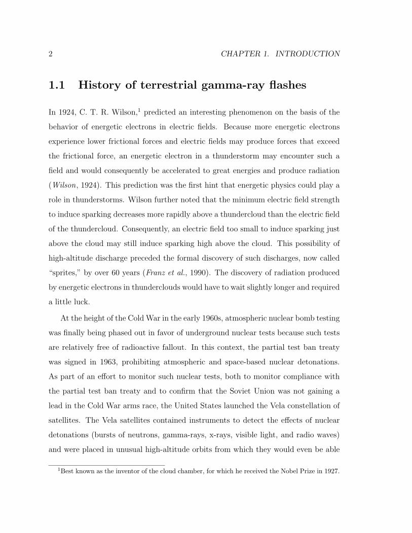
1.1 History of terrestrial gamma-ray flashes
In 1924, C. T. R. Wilson,1 predicted an interesting phenomenon on the basis of the
behavior of energetic electrons in electric fields. Because more energetic electrons
experience lower frictional forces and electric fields may produce forces that exceed
the frictional force, an energetic electron in a thunderstorm may encounter such a
field and would consequently be accelerated to great energies and produce radiation
(Wilson, 1924). This prediction was the first hint that energetic physics could play a
role in thunderstorms. Wilson further noted that the minimum electric field strength
to induce sparking decreases more rapidly above a thundercloud than the electric field
of the thundercloud. Consequently, an electric field too small to induce sparking just
above the cloud may still induce sparking high above the cloud. This possibility of
high-altitude discharge preceded the formal discovery of such discharges, now called
“sprites,” by over 60 years (Franz et al., 1990). The discovery of radiation produced
by energetic electrons in thunderclouds would have to wait slightly longer and required
a little luck.
At the height of the Cold War in the early 1960s, atmospheric nuclear bomb testing
was finally being phased out in favor of underground nuclear tests because such tests
are relatively free of radioactive fallout. In this context, the partial test ban treaty
was signed in 1963, prohibiting atmospheric and space-based nuclear detonations.
As part of an effort to monitor such nuclear tests, both to monitor compliance with
the partial test ban treaty and to confirm that the Soviet Union was not gaining a
lead in the Cold War arms race, the United States launched the Vela constellation of
satellites. The Vela satellites contained instruments to detect the effects of nuclear
detonations (bursts of neutrons, gamma-rays, x-rays, visible light, and radio waves)
and were placed in unusual high-altitude orbits from which they would even be able
1Best known as the inventor of the cloud chamber, for which he received the Nobel Prize in 1927.
1.1. HISTORY OF TERRESTRIAL GAMMA-RAY FLASHES 3
to detect nuclear tests on the far side of the Moon. Though the satellites did not
detect any nuclear tests,2 they did detect bursts of gamma-rays originating outside
the solar system. These observations are now recognized as the discovery of cosmic
gamma-ray bursts, first published by Klebesadel et al. (1973).
These cosmic gamma-ray bursts, being some of the most energetic explosions in
the entire universe, then became the subject of intense study. Though a wide range
of behaviors are observed, a typical gamma-ray burst lasts a few seconds and in
those seconds releases more energy than a typical star in its entire lifetime. Many
theories have been developed to explain these intense bursts, ranging from the collapse
of massive stars to star-quakes on highly-magnetized neutron stars (magnetars). A
review can be found in Fishman and Meegan (1995).
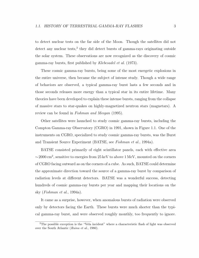
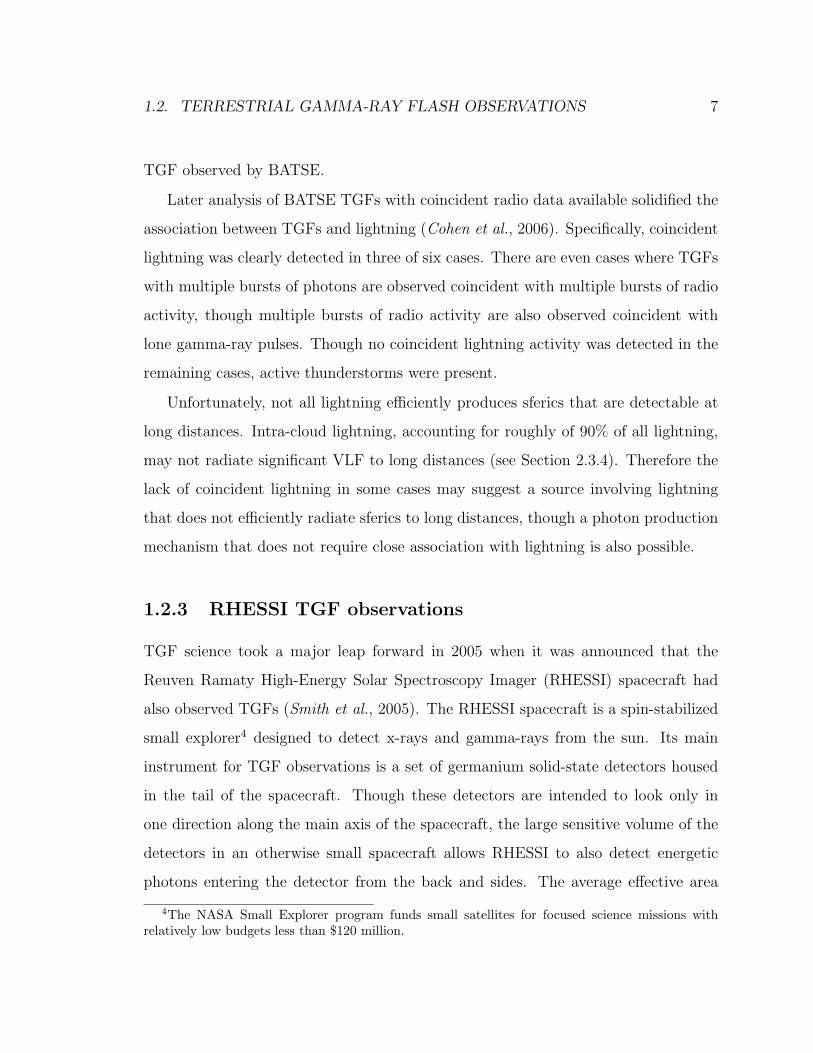
Other satellites were launched to study cosmic gamma-ray bursts, including the
Compton Gamma-ray Observatory (CGRO) in 1991, shown in Figure 1.1. One of the
instruments on CGRO, specialized to study cosmic gamma-ray bursts, was the Burst
and Transient Source Experiment (BATSE, see Fishman et al., 1994a).
BATSE consisted primarily of eight scintillator panels, each with effective area
∼2000 cm2, sensitive to energies from 25 keV to above 1 MeV, mounted on the corners
of CGRO facing outward as on the corners of a cube. As such, BATSE could determine
the approximate direction toward the source of a gamma-ray burst by comparison of
radiation levels at different detectors. BATSE was a wonderful success, detecting
hundreds of cosmic gamma-ray bursts per year and mapping their locations on the
sky (Fishman et al., 1994a).
It came as a surprise, however, when anomalous bursts of radiation were observed
only by detectors facing the Earth. These bursts were much shorter than the typi-
cal gamma-ray burst, and were observed roughly monthly, too frequently to ignore.
2The possible exception is the “Vela incident” where a characteristic flash of light was observedover the South Atlantic (Ruina et al., 1980).
4 CHAPTER 1. INTRODUCTION
Figure 1.1: A schematic of the Compton Gamma-Ray Observatory. TheBurst And Transient Source Experiment (BATSE) modules are mounted near thecorners of the main body of the spacecraft. The six visible modules of eight areindicated with arrows. Figure credit: NASA, GSFC, P.J.T. Leonard.
These observations are now recognized as the discovery of a new class of phenom-
ena known as terrestrial gamma-ray flashes (TGFs, Fishman et al., 1994b). Though
unexpected, these bursts of energetic radiation appeared to be the confirmation of
Wilson’s predictions 70 years earlier that energetic radiation would be emitted above
thunderstorms. Despite the prescience of Wilson’s basic predictions, the physical
picture of TGFs as short bursts of energetic photons was incomplete and required
further study.
1.2 Terrestrial gamma-ray flash observations
1.2.1 BATSE TGF observations
BATSE’s large detectors, limited storage space and limited telemetry bandwidth re-
quired a triggering scheme to limit data collection to just the most interesting events.
As such, the BATSE data focuses on events with intensities far above the background
noise. Such events would trigger the data acquisition system which would then store
1.2. TERRESTRIAL GAMMA-RAY FLASH OBSERVATIONS 5
0 10 20t (ms)
1457
0 10 20
2457
0
0.2
0.4
0.6
0.8
1
dN
/dt
(rel
.unit
s)
0 10 20
106
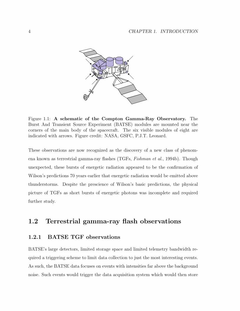
Figure 1.2: Sample BATSE TGFs. The y axis represents count rate of 25–1000 keVphotons, while the x axis is time in milliseconds. The trigger number from the BATSEcatalog is shown in the upper left. Data from the Compton Observatory ScienceSupport Center (COSSC) data archive at http://cossc.gsfc.nasa.gov.
every photon detected by the instrument as an arrival time and an energy in one of
four energy bins (25–50, 50–100, 100–300, and >300 keV with sensitivity decreasing
above 1 MeV). BATSE data thus shows TGFs as short bursts of up to 1000 photons
with energies ranging from 25 keV up to above 1 MeV. BATSE observed 76 TGFs
over its 9-year lifetime.3
Several BATSE TGFs are shown in Figure 1.2. Even in just three events, a wide
range of behavior can be seen, with bursts ranging from less than one to greater than
five milliseconds. The observed fluence ranges from 0.1–0.5 photons/cm2. Typically, a
single pulse is seen, but groups of seven or more pulses separated by a few milliseconds
have also been observed.
This wide range of behavior is difficult to explain with any one physical mech-
anism. Any postulated source mechanism must be able to explain both bursts less
than 1 ms and bursts longer than 8 ms. The question of how multiple pulses may be
produced in a short time is also a puzzle.
3A complete list of BATSE TGF observations can be found at http://www.batse.msfc.nasa.gov/batse/tgf/.
6 CHAPTER 1. INTRODUCTION
Though the initial BATSE TGF data provide little more than a picture of TGFs
as rare, short, and atmospheric, several useful inferences can be made. Analysis of
the shape of the light curves shows that the minimum variability timescale associated
with the emissions requires a source region smaller than 7 km to account for the rapid
variations in intensity in some especially short-duration cases (Nemiroff et al., 1997).
The BATSE data also shows significant numbers of photons with energy < 50 keV.
As photons with energy < 50 keV are heavily attenuated in air, these photons must
come from at least 30 km altitude, suggesting a high-altitude source (Fishman et al.,
1994b). Though the four channel spectral information in the BATSE data is crude,
the spectra recorded are consistent with photons produced by energetic electrons,
leading Fishman et al. (1994b) to suggest production associated with high-altitude
lightning.
1.2.2 BATSE TGFs and coincident lightning observations
The suggestion that lightning may be associated with TGFs was subsequently sup-
ported by lightning observations. As discussed in Section 2.3.4, cloud-to-ground light-
ning activity emits radio waves primarily in the very low frequency (VLF) band from
3 to 30 kHz (Rakov and Uman, 2003, p. 443). These signals propagate very efficiently
in a waveguide formed between the Earth and the conducting upper atmosphere (the
ionosphere), and can be detected thousands of kilometers from the source lightning.
The direction from receiver to source and the relative arrival time of the signal at
multiple receivers can be used to determine the location of the source lightning. Ex-
amination of radio recordings taken during time periods when TGFs were observed
therefore provides a way to examine cloud-to-ground lightning activity possibly asso-
ciated with TGF production. Inan et al. (1996) made such observations and found
active thunderstorm systems near CGRO for two TGFs. In one case, a radio signal
from lightning (a radio atmospheric or “sferic”) was observed within ±1.5 ms of the
1.2. TERRESTRIAL GAMMA-RAY FLASH OBSERVATIONS 7
TGF observed by BATSE.
Later analysis of BATSE TGFs with coincident radio data available solidified the
association between TGFs and lightning (Cohen et al., 2006). Specifically, coincident
lightning was clearly detected in three of six cases. There are even cases where TGFs
with multiple bursts of photons are observed coincident with multiple bursts of radio
activity, though multiple bursts of radio activity are also observed coincident with
lone gamma-ray pulses. Though no coincident lightning activity was detected in the
remaining cases, active thunderstorms were present.
Unfortunately, not all lightning efficiently produces sferics that are detectable at
long distances. Intra-cloud lightning, accounting for roughly of 90% of all lightning,
may not radiate significant VLF to long distances (see Section 2.3.4). Therefore the
lack of coincident lightning in some cases may suggest a source involving lightning
that does not efficiently radiate sferics to long distances, though a photon production
mechanism that does not require close association with lightning is also possible.
1.2.3 RHESSI TGF observations
TGF science took a major leap forward in 2005 when it was announced that the
Reuven Ramaty High-Energy Solar Spectroscopy Imager (RHESSI) spacecraft had
also observed TGFs (Smith et al., 2005). The RHESSI spacecraft is a spin-stabilized
small explorer4 designed to detect x-rays and gamma-rays from the sun. Its main
instrument for TGF observations is a set of germanium solid-state detectors housed
in the tail of the spacecraft. Though these detectors are intended to look only in
one direction along the main axis of the spacecraft, the large sensitive volume of the
detectors in an otherwise small spacecraft allows RHESSI to also detect energetic
photons entering the detector from the back and sides. The average effective area
4The NASA Small Explorer program funds small satellites for focused science missions withrelatively low budgets less than $120 million.
8 CHAPTER 1. INTRODUCTION
for such detection of photons with energies above 50 keV is ∼242 cm2 (Smith, 2006).
Unlike BATSE, all photons detected are stored and transmitted to ground without
need for a trigger.
RHESSI provides a novel view of TGFs. Without the requirement of a trigger,
RHESSI collects a large data set to be mined for TGFs. RHESSI is thus found to
observe TGFs much more frequently than BATSE, detecting one every several days,
compared with BATSE observations of approximately one per month.5 RHESSI also
collects higher resolution photon energy information than the four-channel spectra
produced by BATSE. RHESSI does not provide directional information, only iden-
tifying TGFs on the basis of duration; 1 ms TGFs are much shorter than typical
gamma-ray bursts. Though gamma-ray bursts are occasionally as short as 1 ms (see
for instance Figure 1 of Lee et al. (2000)) and RHESSI does occasionally trigger on
short pulses from soft gamma-ray repeaters, such events as identified by other satel-
lites are removed from the set of TGFs (Smith, 2009). RHESSI also has a much
smaller effective area than BATSE so it does not collect as many photons, typically
< 100 photons per TGF. Such small numbers of photons limit analysis of RHESSI
spectra to averages over many TGFs.
The greater frequency of RHESSI TGF observations requires a global frequency of
at least 50 /day given the optimistic assumption that TGFs are detectable if produced
less than 1000 km from the subsatellite point (Smith et al., 2005). The more realistic
assumption that TGFs are only detectable if produced less than 300 km from the
subsatellite point gives a global frequency of approximately 500 /day. Compared to
the global lightning frequency of ∼ 40 /second, it can therefore be estimated that 1
in approximately 104 lightning discharges produces a TGF. The better statistics also
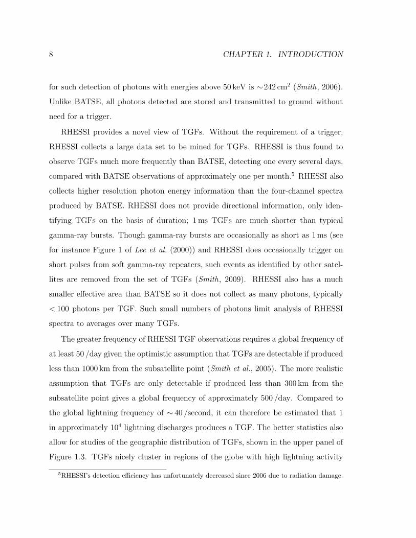
allow for studies of the geographic distribution of TGFs, shown in the upper panel of
Figure 1.3. TGFs nicely cluster in regions of the globe with high lightning activity
5RHESSI’s detection efficiency has unfortunately decreased since 2006 due to radiation damage.
1.2. TERRESTRIAL GAMMA-RAY FLASH OBSERVATIONS 9
Figure 1.3: RHESSI TGF and LIS lightning map. Upper panel: map showingthe location of the RHESSI satellite when TGFs were observed. The dashed linesindicate the typical regions of coverage limited by the 38 orbital inclination and theradiation conditions in the South Atlantic Anomaly. Lower panel: global lightningdistribution as seen by the Lightning Imaging Sensor. Darker colors indicate higherflash density. Clusters of TGFs are seen in regions of high lightning activity: Centraland South America, Central Africa, Southeast Asia, and Oceania. Data courtesy ofD. Smith taken from the RHESSI TGF data archive at http://scipp.ucsc.edu/
~dsmith/tgflib_public/ and the Lightning Imaging Sensor data server at http:
//thunder.msfc.nasa.gov/data/.
as seen by the Lightning Imaging Sensor (Christian et al., 1999), shown in the lower
panel of Figure 1.3.
10 CHAPTER 1. INTRODUCTION
10−2
10−1
100
101Ed
N/dE
(arb
.unit
s)
10−2 10−1 100 101
energy (MeV)
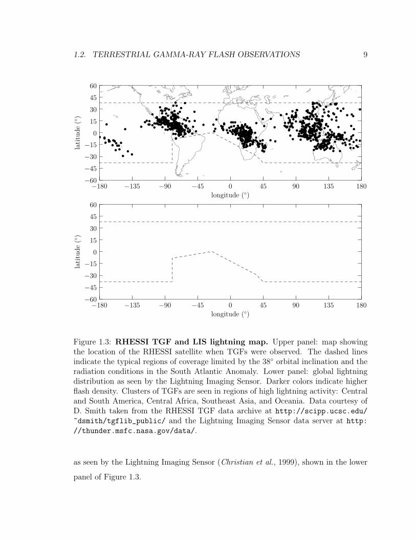
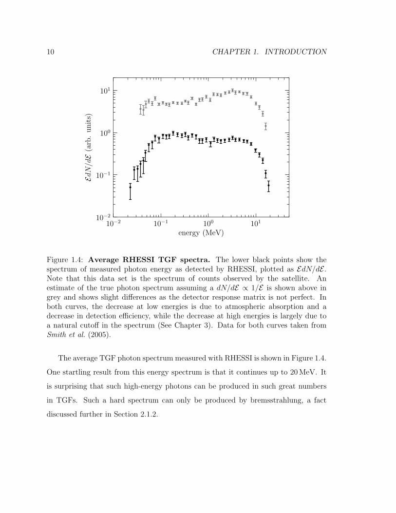
Figure 1.4: Average RHESSI TGF spectra. The lower black points show thespectrum of measured photon energy as detected by RHESSI, plotted as EdN/dE .Note that this data set is the spectrum of counts observed by the satellite. Anestimate of the true photon spectrum assuming a dN/dE ∝ 1/E is shown above ingrey and shows slight differences as the detector response matrix is not perfect. Inboth curves, the decrease at low energies is due to atmospheric absorption and adecrease in detection efficiency, while the decrease at high energies is largely due toa natural cutoff in the spectrum (See Chapter 3). Data for both curves taken fromSmith et al. (2005).
The average TGF photon spectrum measured with RHESSI is shown in Figure 1.4.
One startling result from this energy spectrum is that it continues up to 20 MeV. It
is surprising that such high-energy photons can be produced in such great numbers
in TGFs. Such a hard spectrum can only be produced by bremsstrahlung, a fact
discussed further in Section 2.1.2.
1.2. TERRESTRIAL GAMMA-RAY FLASH OBSERVATIONS 11
1.2.4 RHESSI TGFs and coincident lightning observations
Lightning associated with RHESSI TGFs has been studied very successfully due to
the large number of TGFs detected. Extension of the studies of Inan et al. (1996)
and Cohen et al. (2006) to RHESSI TGFs for which lightning data is available show
coincident lightning activity within several milliseconds for 76% of TGFs, much higher
than the ∼2% expected by random chance (Inan et al., 2006). The coincident radio
signals detected in Inan et al. (2006) indicate that the associated lightning discharge
often has unusually high peak current, especially for TGFs observed over the ocean,
but the association is not perfect. This result suggests relatively intense discharges,
though a complete picture of lightning activity is not provided by distant VLF mea-
surements. In particular, the role of intra-cloud discharges is not resolved and may
be relevant to TGF production. Though the timing of coincident lightning relative to
satellite observation is difficult to determine due to timing uncertainty in the RHESSI
spacecraft, the relative timing is consistent with geometric effects and measurement
error provided that an additional 2 ms variance is allowed for other effects. Further
analysis involving accurate geolocations of lightning associated with 34 TGFs (de-
scribed in Cohen et al., 2009) indicates that the distance between lightning and the
subsatellite point is typically <300 km, consistent with similar analyses by Cummer
et al. (2005). The timing coincidence between TGF and associated lightning is also
much closer when the geometric uncertainty can be resolved with known lightning lo-
cations. The remaining timing spread is consistent with poor timing on the RHESSI
satellite and the additional 2 ms variance mentioned above. Note that the additional
2 ms variance observed between the time of TGF production and the time of sferic
emission does not result from measurement error, and thus implies some displacement
in time and/or space between the sferic and TGF sources.
Some light was shed on the question of the specific lightning processes possibly
associated with TGFs by Stanley et al. (2006). Though their sample of 6 geolocated
12 CHAPTER 1. INTRODUCTION
lightning discharges associated with TGFs is smaller and therefore less useful than
those described in Cohen et al. (2009), the radio signals received for two of the cases
reported by Stanley et al. (2006) came from lightning that was close enough to their
receiver and rapid enough to show ionospheric reflections. In such cases, the relative
timing of the direct and reflected signals can be used to infer the altitude of the
source of the radio signal. The altitudes were measured to be 13.6 km and 11.5 km.
These altitudes are too high to be produced by cloud-to-ground lightning, strongly
suggesting that these two cases were associated with intra-cloud discharge.
1.2.5 Summary of TGF observations
These satellite observations of TGFs and analysis of coincident lightning activity
seen in radio observations provide a reasonably clear picture of the phenomenon of
terrestrial gamma-ray flashes. TGFs as observed on satellites are short, ranging from
less than one to several milliseconds with one or more pulses observed separated by a
few milliseconds. The photons themselves have a very hard spectrum with a maximum
energy at or above 20 MeV, strongly suggesting a bremsstrahlung source. The overall
fluence observed is approximately 1 photon/cm2. Radio observations coincident with
satellite TGF detections typically show lightning activity within several milliseconds.
When the lightning activity can be geolocated, it is typically less than 300 km from the
subsatellite point. Not all TGFs are associated with detectable VLF radio activity,
which together with the observations of source heights above 10 km by Stanley et al.
(2006) suggests intra-cloud lightning as the source of some TGFs. Closer scrutiny of
the radio emissions associated with TGFs shows a slight tendency toward discharges
with high peak current (Inan et al., 2006).
1.3. MOTIVATION 13
1.3 Motivation
TGFs have attracted a great deal of attention since their discovery. This attention
stems from the novelty of the subject and the implications of energetic processes for
such common phenomena as thunderstorms and lightning.
The presence of 20 MeV photons in a TGF is quite remarkable. Such energetic
photons cannot be produced by radioactive decay, and therefore require a physical
process akin to a natural particle accelerator. That such a particle accelerator may
exist in or above thunderstorms is a fascinating development and poses an irresistible
puzzle for atmospheric physics.
Even given such a particle accelerator, the production of sufficient numbers of
energetic photons to produce an observable TGF is by no means an obvious con-
sequence. How much energy is required, and where and how that energy must be
produced are also interesting questions.
The timing of TGFs also poses an interesting puzzle. If a typical TGF lasts 1 ms,
the source process must also last approximately 1 ms. A typical lightning discharge,
by contrast, has a total duration from initiation to quiescence of several hundred mil-
liseconds, while the relaxation timescale for electric fields in air ranges from 0.1–10 s.
TGFs must therefore be associated with very dynamic processes occurring as small
portions of the lightning discharge as a whole. The precise nature of these processes
and how they are associated with TGF production is an essential unanswered question
that motivates TGF research.
The energetic processes that must occur in a TGF have direct implications for
many processes in the Earth’s atmosphere. Lightning, clearly associated with TGFs,
itself is poorly-understood. Present understanding of lightning physics does not in-
clude the processes necessary for TGF production, so studies of TGF physics may
help advance the understanding of lightning. The unknown mechanism of lightning
14 CHAPTER 1. INTRODUCTION
initiation, one of the main open questions in thunderstorm dynamics, may also be
influenced by processes involved in TGF production. The contribution of TGFs to
the atmosphere and space radiation environment and the chemical effects of energetic
processes in the atmosphere are also of great interest. The possibility of addressing
these open questions motivates the studies of TGFs described herein.
1.4 Contributions
This dissertation addresses several of the open questions listed above and attempts
to explain relevant aspects of TGF physics. The investigations described in the sub-
sequent chapters follow from the theory of the physics involved in TGF production
as described in Chapter 2. In particular, the physics of relativistic electrons driven
by electric fields in materials (i.e., air) is central to the studies described in this work.
Existing theoretical mechanisms of TGF production are also discussed in Chapter 2.
The fact that these theories are unable to explain TGF observations directly motivates
our investigations.
The specific contributions of this dissertation are:
1. Development of constraints on properties of the TGF photon source by com-
parison of Monte Carlo simulation results with satellite data. These results
constrain the TGF source altitude, energy, and directional distribution (Chap-
ter 3).
2. Determination of the production and properties of energetic electrons by cosmic
rays in the Earth’s atmosphere and simulate the behavior of such electrons in
electric fields by Monte Carlo techniques. These results set further requirements
on the source of TGF photons (Chapter 4).
3. Conception and development of a new mechanism for TGF production driven
1.4. CONTRIBUTIONS 15
directly by lightning current pulses. This mechanism meets the requirements
described by the previous two contributions, and allows construction of testable
predictions (Chapter 5).
4. Modeling of the mechanism of TGF production by lightning current pulses by
use of the method of moments and Monte Carlo simulations. This model is
then used to derive requirements on TGF-associated lightning (Chapter 6).
This dissertation as a whole therefore provides a set of clear requirements on
TGF production mechanisms, provides a mechanism that attempts to meet these
requirements, and presents a model of this mechanism that determines the conditions
under which it can successfully reproduce TGF observations.
Chapter 2
Theoretical background
Though terrestrial gamma-ray flashes pose an interesting puzzle, the physical phe-
nomena involved in TGF production have been well-studied both experimentally and
theoretically. A broad understanding of TGF production can be derived from the
presence of 20 MeV photons. The behavior of energetic photons in a TGF as they
propagate through the atmosphere is governed by three processes: photoelectric ab-
sorption, Compton scattering, and pair production. Such photons can only be pro-
duced by acceleration of energetic electrons undergoing collisions, a process known
as bremsstrahlung.1 The behavior of the energetic electrons necessary for brems-
strahlung depends on the electron energy but largely reduces to simple collisional
processes. The electric field necessary to accelerate electrons to high energies allows
for additional interesting phenomena which draw energy from the electric field. The
electric fields come from thunderstorms and lightning, phenomena that are crucial to
the production of TGFs. These processes are described in detail in this chapter.
1“Braking radiation” in German.
16
2.1. ENERGETIC PARTICLE DYNAMICS 17
10−2
10−1
100
101
102
103
104
105
cros
sse
ctio
n(b
)
10−3 10−2 10−1 100 101 102 103
energy (MeV)
photoelectric
Comptonpair
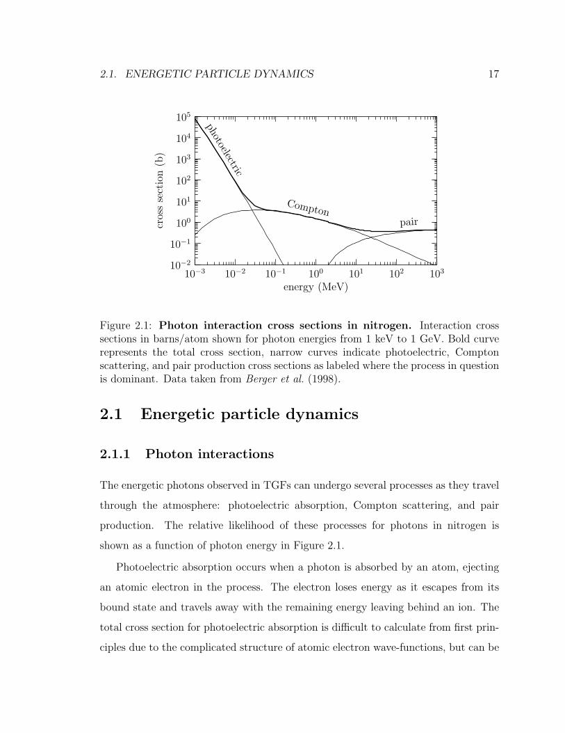
Figure 2.1: Photon interaction cross sections in nitrogen. Interaction crosssections in barns/atom shown for photon energies from 1 keV to 1 GeV. Bold curverepresents the total cross section, narrow curves indicate photoelectric, Comptonscattering, and pair production cross sections as labeled where the process in questionis dominant. Data taken from Berger et al. (1998).
2.1 Energetic particle dynamics
2.1.1 Photon interactions
The energetic photons observed in TGFs can undergo several processes as they travel
through the atmosphere: photoelectric absorption, Compton scattering, and pair
production. The relative likelihood of these processes for photons in nitrogen is
shown as a function of photon energy in Figure 2.1.
Photoelectric absorption occurs when a photon is absorbed by an atom, ejecting
an atomic electron in the process. The electron loses energy as it escapes from its
bound state and travels away with the remaining energy leaving behind an ion. The
total cross section for photoelectric absorption is difficult to calculate from first prin-
ciples due to the complicated structure of atomic electron wave-functions, but can be
18 CHAPTER 2. THEORETICAL BACKGROUND
approximated for photon energies above the binding energy of the K-shell electrons
but below the electron rest energy as:
σphoto =32√
2α4r2eZ
5
3
(mec
2
hν
)7/2
(2.1)
where α is the fine structure constant, re is the classical electron radius, Z is the
atomic number, me is the electron rest mass, c is the speed of light, h is Planck’s
constant, and ν is the frequency of the incident photon (Leo, 1994, p. 54–55). As
photon energy hν increases, the cross section decreases rapidly as (hν)−7/2.
As can be seen in Figure 2.1, for energies above ∼ 30 keV Compton scattering
becomes the dominant process for energetic photons in nitrogen.2 Compton scattering
occurs when an incident photon scatters off and imparts some of its energy to an
electron. Both the scattered photon and the recoil electron emerge from the collision.
The final energy of the photon hν ′ depends on the scattering angle θ and can be
calculated as a homework problem in special relativity:
hν ′ =hν
1 + γ(1− cos θ)(2.2)
where γ = hν/mec2. This collision leaves the recoil electron with a kinetic energy T
given by
T = hν − hν ′ = hνγ(1− cos θ)
1 + γ(1− cos θ)(2.3)
The cross section for Compton scattering can be calculated to lowest order from
elementary quantum electrodynamics and is referred to as the Klein-Nishina cross
section:dσ
dΩ=r2e
2
1
[1 + γ(1− cos θ)]2
[1 + cos2 θ +
γ2(1− cos θ)2
1 + γ(1− cos θ)2
](2.4)
2Note the very strong Z dependence in Equation 2.1 Elements with higher atomic number havemuch greater photoelectric absorption cross sections and therefore Compton scattering only becomesimportant for relatively larger energies.
2.1. ENERGETIC PARTICLE DYNAMICS 19
where the cross section is given as a differential in solid angle Ω. For a detailed
derivation, see Peskin and Schroeder (1995, pp 158–167). The total cross section can
be obtained by integrating over solid angle to yield
σc = 2πr2e
1 + γ
γ2
[2(1 + γ)
1 + 2γ− ln(1 + 2γ)
γ
]+
ln(1 + 2γ)
2γ− 1 + 3γ
(1 + 2γ)2
(2.5)
For large photon energy, the terms in Equation 2.5 have roughly 1/γ dependence,
leading the Compton scattering cross section to drop off at relativistic energies.
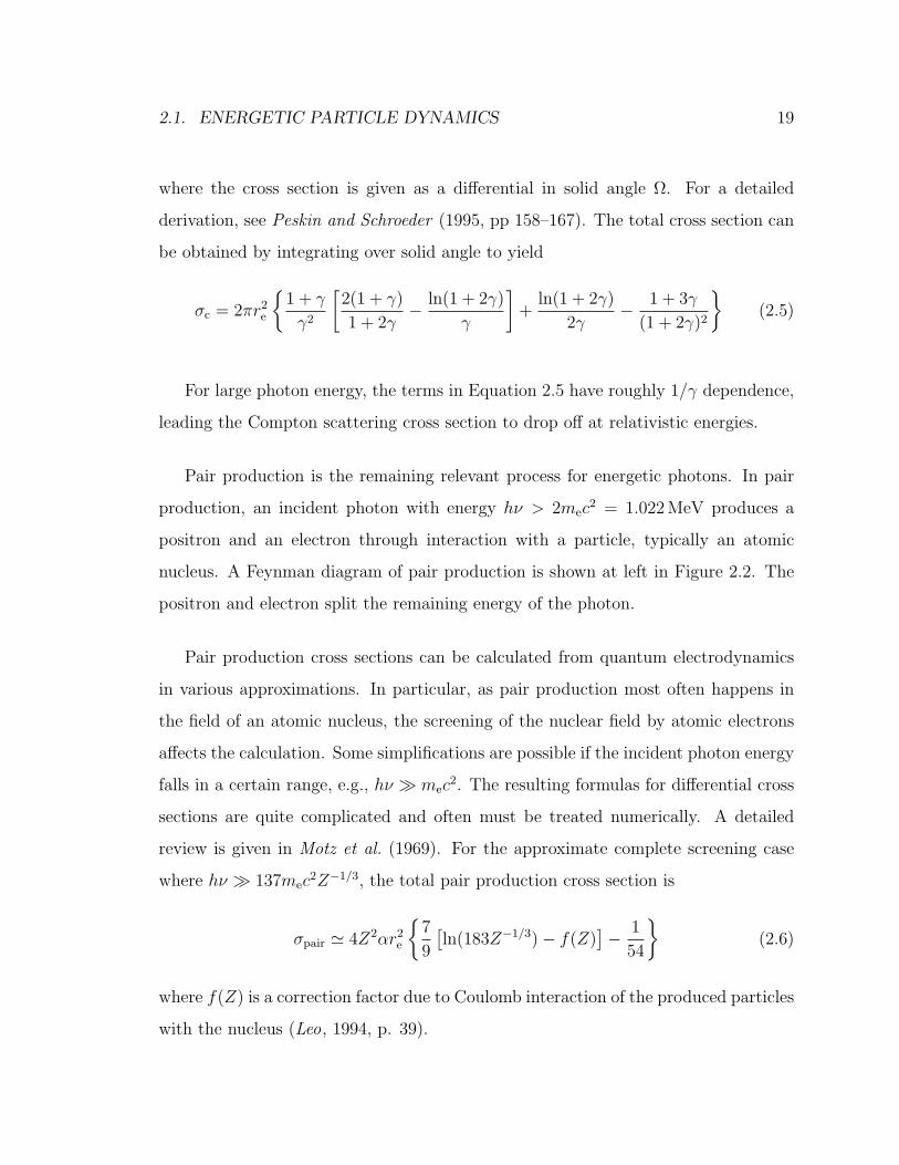
Pair production is the remaining relevant process for energetic photons. In pair
production, an incident photon with energy hν > 2mec2 = 1.022 MeV produces a
positron and an electron through interaction with a particle, typically an atomic
nucleus. A Feynman diagram of pair production is shown at left in Figure 2.2. The
positron and electron split the remaining energy of the photon.
Pair production cross sections can be calculated from quantum electrodynamics
in various approximations. In particular, as pair production most often happens in
the field of an atomic nucleus, the screening of the nuclear field by atomic electrons
affects the calculation. Some simplifications are possible if the incident photon energy
falls in a certain range, e.g., hν mec2. The resulting formulas for differential cross
sections are quite complicated and often must be treated numerically. A detailed
review is given in Motz et al. (1969). For the approximate complete screening case
where hν 137mec2Z−1/3, the total pair production cross section is
σpair ' 4Z2αr2e
7
9
[ln(183Z−1/3)− f(Z)
]− 1
54
(2.6)
where f(Z) is a correction factor due to Coulomb interaction of the produced particles
with the nucleus (Leo, 1994, p. 39).
20 CHAPTER 2. THEORETICAL BACKGROUND
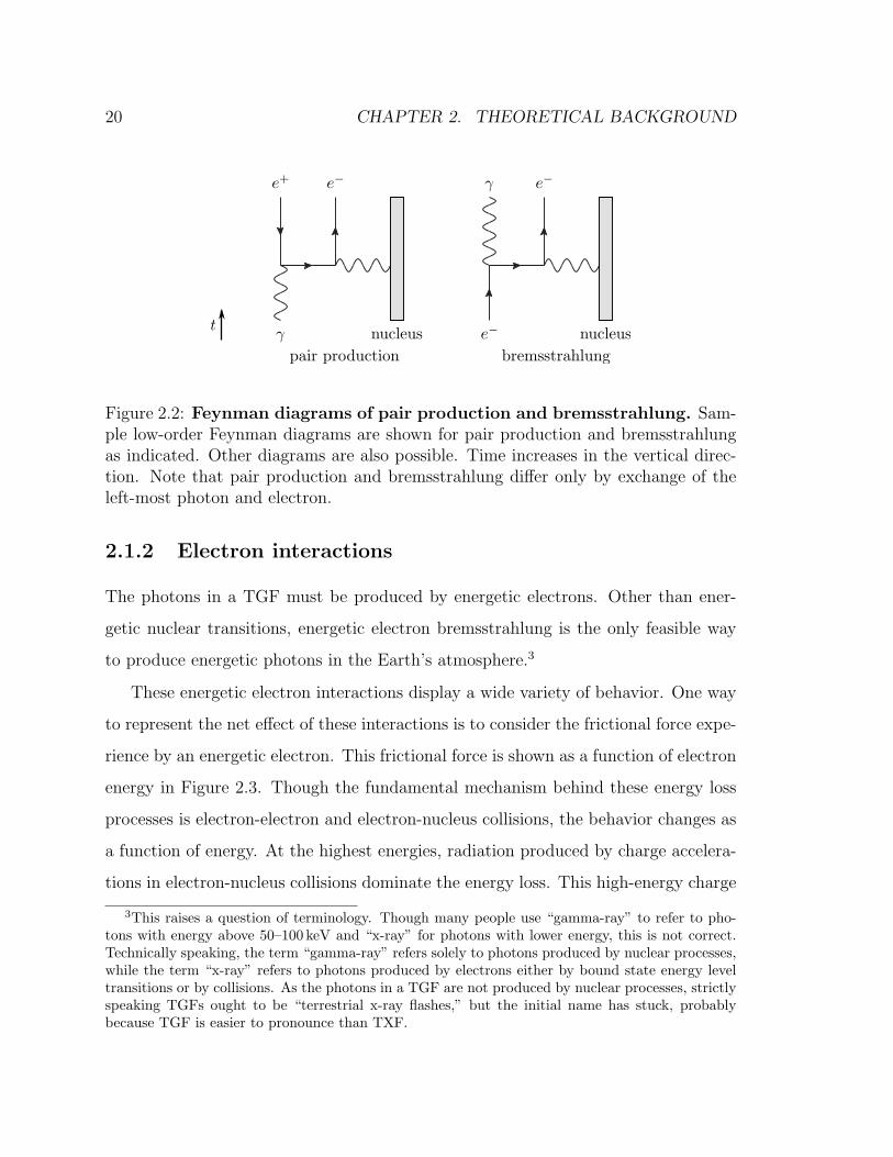
Figure 2.2: Feynman diagrams of pair production and bremsstrahlung. Sam-ple low-order Feynman diagrams are shown for pair production and bremsstrahlungas indicated. Other diagrams are also possible. Time increases in the vertical direc-tion. Note that pair production and bremsstrahlung differ only by exchange of theleft-most photon and electron.
2.1.2 Electron interactions
The photons in a TGF must be produced by energetic electrons. Other than ener-
getic nuclear transitions, energetic electron bremsstrahlung is the only feasible way
to produce energetic photons in the Earth’s atmosphere.3
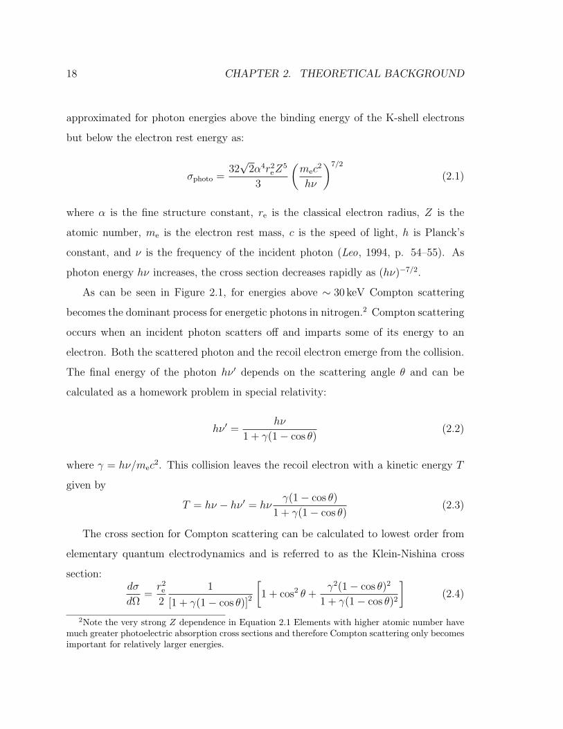
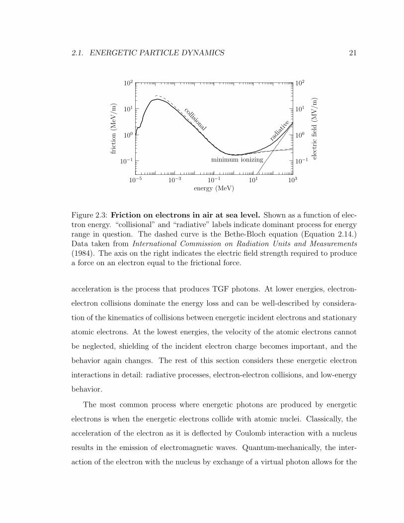
These energetic electron interactions display a wide variety of behavior. One way
to represent the net effect of these interactions is to consider the frictional force expe-
rience by an energetic electron. This frictional force is shown as a function of electron
energy in Figure 2.3. Though the fundamental mechanism behind these energy loss
processes is electron-electron and electron-nucleus collisions, the behavior changes as
a function of energy. At the highest energies, radiation produced by charge accelera-
tions in electron-nucleus collisions dominate the energy loss. This high-energy charge
3This raises a question of terminology. Though many people use “gamma-ray” to refer to pho-tons with energy above 50–100 keV and “x-ray” for photons with lower energy, this is not correct.Technically speaking, the term “gamma-ray” refers solely to photons produced by nuclear processes,while the term “x-ray” refers to photons produced by electrons either by bound state energy leveltransitions or by collisions. As the photons in a TGF are not produced by nuclear processes, strictlyspeaking TGFs ought to be “terrestrial x-ray flashes,” but the initial name has stuck, probablybecause TGF is easier to pronounce than TXF.
2.1. ENERGETIC PARTICLE DYNAMICS 21
10−1
100
101
102
elec
tric
fiel
d(M
V/m
)
10−1
100
101
102
fric
tion
(MeV
/m)
10−5 10−3 10−1 101 103
energy (MeV)
collisional
radiative
minimum ionizing
Figure 2.3: Friction on electrons in air at sea level. Shown as a function of elec-tron energy. “collisional” and “radiative” labels indicate dominant process for energyrange in question. The dashed curve is the Bethe-Bloch equation (Equation 2.14.)Data taken from International Commission on Radiation Units and Measurements(1984). The axis on the right indicates the electric field strength required to producea force on an electron equal to the frictional force.
acceleration is the process that produces TGF photons. At lower energies, electron-
electron collisions dominate the energy loss and can be well-described by considera-
tion of the kinematics of collisions between energetic incident electrons and stationary
atomic electrons. At the lowest energies, the velocity of the atomic electrons cannot
be neglected, shielding of the incident electron charge becomes important, and the
behavior again changes. The rest of this section considers these energetic electron
interactions in detail: radiative processes, electron-electron collisions, and low-energy
behavior.
The most common process where energetic photons are produced by energetic
electrons is when the energetic electrons collide with atomic nuclei. Classically, the
acceleration of the electron as it is deflected by Coulomb interaction with a nucleus
results in the emission of electromagnetic waves. Quantum-mechanically, the inter-
action of the electron with the nucleus by exchange of a virtual photon allows for the
22 CHAPTER 2. THEORETICAL BACKGROUND
emission of a real photon with nonzero amplitude as calculated in quantum electrody-
namics. A Feynman diagram of bremsstrahlung is shown at right in Figure 2.2. In the
context of quantum electrodynamics, bremsstrahlung and pair production are related
by rearrangements of particles in time. Pair production involves an outgoing positron
and an incoming photon, while bremsstrahlung involves an incoming electron and an
outgoing photon. The cross section formulas for bremsstrahlung are thus derived
similarly to pair production formulas and are similarly complicated and depend on
similar approximations. A detailed review is given in Koch and Motz (1959).
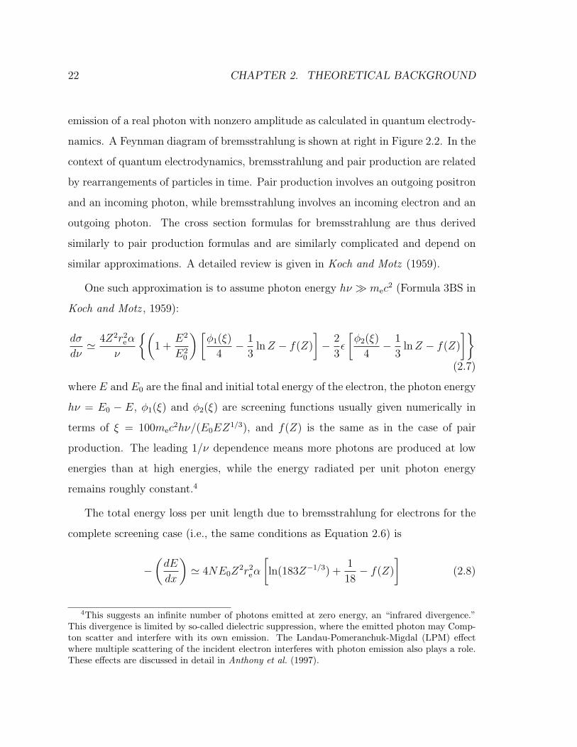
One such approximation is to assume photon energy hν mec2 (Formula 3BS in
Koch and Motz , 1959):
dσ
dν' 4Z2r2
eα
ν
(1 +
E2
E20
)[φ1(ξ)
4− 1
3lnZ − f(Z)
]− 2
3ε
[φ2(ξ)
4− 1
3lnZ − f(Z)
](2.7)
where E and E0 are the final and initial total energy of the electron, the photon energy
hν = E0 − E, φ1(ξ) and φ2(ξ) are screening functions usually given numerically in
terms of ξ = 100mec2hν/(E0EZ
1/3), and f(Z) is the same as in the case of pair
production. The leading 1/ν dependence means more photons are produced at low
energies than at high energies, while the energy radiated per unit photon energy
remains roughly constant.4
The total energy loss per unit length due to bremsstrahlung for electrons for the
complete screening case (i.e., the same conditions as Equation 2.6) is
−(dE
dx
)' 4NE0Z
2r2eα
[ln(183Z−1/3) +
1
18− f(Z)
](2.8)
4This suggests an infinite number of photons emitted at zero energy, an “infrared divergence.”This divergence is limited by so-called dielectric suppression, where the emitted photon may Comp-ton scatter and interfere with its own emission. The Landau-Pomeranchuk-Migdal (LPM) effectwhere multiple scattering of the incident electron interferes with photon emission also plays a role.These effects are discussed in detail in Anthony et al. (1997).
2.1. ENERGETIC PARTICLE DYNAMICS 23
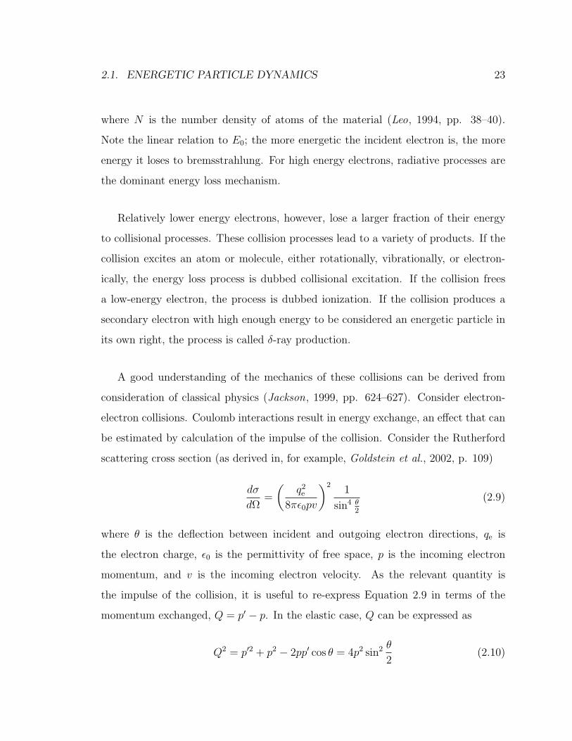
where N is the number density of atoms of the material (Leo, 1994, pp. 38–40).
Note the linear relation to E0; the more energetic the incident electron is, the more
energy it loses to bremsstrahlung. For high energy electrons, radiative processes are
the dominant energy loss mechanism.
Relatively lower energy electrons, however, lose a larger fraction of their energy
to collisional processes. These collision processes lead to a variety of products. If the
collision excites an atom or molecule, either rotationally, vibrationally, or electron-
ically, the energy loss process is dubbed collisional excitation. If the collision frees
a low-energy electron, the process is dubbed ionization. If the collision produces a
secondary electron with high enough energy to be considered an energetic particle in
its own right, the process is called δ-ray production.
A good understanding of the mechanics of these collisions can be derived from
consideration of classical physics (Jackson, 1999, pp. 624–627). Consider electron-
electron collisions. Coulomb interactions result in energy exchange, an effect that can
be estimated by calculation of the impulse of the collision. Consider the Rutherford
scattering cross section (as derived in, for example, Goldstein et al., 2002, p. 109)
dσ
dΩ=
(q2e
8πε0pv
)21
sin4 θ2
(2.9)
where θ is the deflection between incident and outgoing electron directions, qe is
the electron charge, ε0 is the permittivity of free space, p is the incoming electron
momentum, and v is the incoming electron velocity. As the relevant quantity is
the impulse of the collision, it is useful to re-express Equation 2.9 in terms of the
momentum exchanged, Q = p′ − p. In the elastic case, Q can be expressed as
Q2 = p′2 + p2 − 2pp′ cos θ = 4p2 sin2 θ
2(2.10)
24 CHAPTER 2. THEORETICAL BACKGROUND
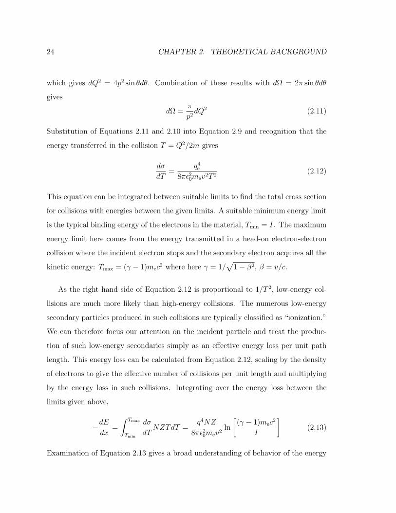
which gives dQ2 = 4p2 sin θdθ. Combination of these results with dΩ = 2π sin θdθ
gives
dΩ =π
p2dQ2 (2.11)
Substitution of Equations 2.11 and 2.10 into Equation 2.9 and recognition that the
energy transferred in the collision T = Q2/2m gives
dσ
dT=
q4e
8πε20mev2T 2(2.12)
This equation can be integrated between suitable limits to find the total cross section
for collisions with energies between the given limits. A suitable minimum energy limit
is the typical binding energy of the electrons in the material, Tmin = I. The maximum
energy limit here comes from the energy transmitted in a head-on electron-electron
collision where the incident electron stops and the secondary electron acquires all the
kinetic energy: Tmax = (γ − 1)mec2 where here γ = 1/
√1− β2, β = v/c.
As the right hand side of Equation 2.12 is proportional to 1/T 2, low-energy col-
lisions are much more likely than high-energy collisions. The numerous low-energy
secondary particles produced in such collisions are typically classified as “ionization.”
We can therefore focus our attention on the incident particle and treat the produc-
tion of such low-energy secondaries simply as an effective energy loss per unit path
length. This energy loss can be calculated from Equation 2.12, scaling by the density
of electrons to give the effective number of collisions per unit length and multiplying
by the energy loss in such collisions. Integrating over the energy loss between the
limits given above,
−dEdx
=
∫ Tmax
Tmin
dσ
dTNZTdT =
q4NZ
8πε20mev2ln
[(γ − 1)mec
2
I
](2.13)
Examination of Equation 2.13 gives a broad understanding of behavior of the energy
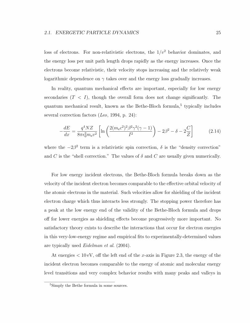
2.1. ENERGETIC PARTICLE DYNAMICS 25
loss of electrons. For non-relativistic electrons, the 1/v2 behavior dominates, and
the energy loss per unit path length drops rapidly as the energy increases. Once the
electrons become relativistic, their velocity stops increasing and the relatively weak
logarithmic dependence on γ takes over and the energy loss gradually increases.
In reality, quantum mechanical effects are important, especially for low energy
secondaries (T < I), though the overall form does not change significantly. The
quantum mechanical result, known as the Bethe-Bloch formula,5 typically includes
several correction factors (Leo, 1994, p. 24):
−dEdx
=q4NZ
8πε20mev2
[ln
(2(mec
2)2β2γ2(γ − 1)
I2
)− 2β2 − δ − 2
C
Z
](2.14)
where the −2β2 term is a relativistic spin correction, δ is the “density correction”
and C is the “shell correction.” The values of δ and C are usually given numerically.
For low energy incident electrons, the Bethe-Bloch formula breaks down as the
velocity of the incident electron becomes comparable to the effective orbital velocity of
the atomic electrons in the material. Such velocities allow for shielding of the incident
electron charge which thus interacts less strongly. The stopping power therefore has
a peak at the low energy end of the validity of the Bethe-Bloch formula and drops
off for lower energies as shielding effects become progressively more important. No
satisfactory theory exists to describe the interactions that occur for electron energies
in this very-low-energy regime and empirical fits to experimentally-determined values
are typically used Eidelman et al. (2004).
At energies < 10 eV, off the left end of the x-axis in Figure 2.3, the energy of the
incident electron becomes comparable to the energy of atomic and molecular energy
level transitions and very complex behavior results with many peaks and valleys in
5Simply the Bethe formula in some sources.
26 CHAPTER 2. THEORETICAL BACKGROUND
the stopping power. A good survey of these interactions, including detailed lists of
the transitions, threshold energies, and final states is given in Moss et al. (2006).
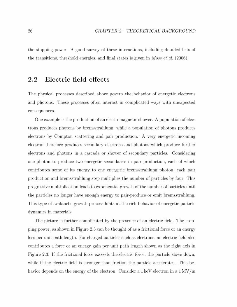
2.2 Electric field effects
The physical processes described above govern the behavior of energetic electrons
and photons. These processes often interact in complicated ways with unexpected
consequences.
One example is the production of an electromagnetic shower. A population of elec-
trons produces photons by bremsstrahlung, while a population of photons produces
electrons by Compton scattering and pair production. A very energetic incoming
electron therefore produces secondary electrons and photons which produce further
electrons and photons in a cascade or shower of secondary particles. Considering
one photon to produce two energetic secondaries in pair production, each of which
contributes some of its energy to one energetic bremsstrahlung photon, each pair
production and bremsstrahlung step multiplies the number of particles by four. This
progressive multiplication leads to exponential growth of the number of particles until
the particles no longer have enough energy to pair-produce or emit bremsstrahlung.
This type of avalanche growth process hints at the rich behavior of energetic particle
dynamics in materials.
The picture is further complicated by the presence of an electric field. The stop-
ping power, as shown in Figure 2.3 can be thought of as a frictional force or an energy
loss per unit path length. For charged particles such as electrons, an electric field also
contributes a force or an energy gain per unit path length shown as the right axis in
Figure 2.3. If the frictional force exceeds the electric force, the particle slows down,
while if the electric field is stronger than friction the particle accelerates. This be-
havior depends on the energy of the electron. Consider a 1 keV electron in a 1 MV/m
2.2. ELECTRIC FIELD EFFECTS 27
electric field in air at sea level. Figure 2.3 shows that for this electron, the fric-
tional force exceeds the electric field force, and the particle will lose energy. A 1 MeV
electron, by contrast, experiences much less friction and the electric force due to a
1 MV/m electric field exceeds the friction force and the particle will accelerate to be-
come what is called a “runaway” electron. The production of such runaway electrons
above thunderstorms was predicted by Wilson (1924) as mentioned in Section 1.1.
2.2.1 Runaway relativistic electron avalanche (RREA)
These runaway electrons continue to interact with the material as they accelerate,
and occasionally will undergo hard electron-electron collisions. These collisions may
impart a significant amount of energy to the secondary electron. If the secondary
electron has enough energy, it too may experience a sufficiently low frictional force to
be accelerated by the electric field and can also be considered a runaway. This multi-
plication in the number of runaway electrons leads to avalanche growth in the popu-
lation of energetic electrons, a process called runaway relativistic electron avalanche
(RREA). This possibility of avalanche growth was first predicted by Gurevich et al.
(1992).
Several properties of RREA are evident from Figure 2.3. First, there is a minimum
energy of runaway electrons given by the point where the electric force equals the
frictional force. For the 1 MV/m electric field mentioned above, this minimum energy
is approximately 30 keV. Second, note that at a given electric field, there is also an
upper limit on runaway electron energy, above which radiative losses dominate and
the particle will lose energy. For instance, a 0.25 MV/m electric field can accelerate
runaway electrons to energies no higher than 20 MeV. Third, electric forces below the
minimum ionizing friction force cannot produce runaway electrons. This minimum
electric field strength is '0.2 MV/m. Note that this minimum electric field strength
is much lower than the minimum electric field necessary to produce sparking, a fact
28 CHAPTER 2. THEORETICAL BACKGROUND
considered in more detail in Section 2.3.3. Fourth, for electric forces stronger than
the maximum frictional force on non-relativistic electrons, i.e., above Ec ' 25 MV/m
for 100 eV electrons, there is no minimum energy of runaway electrons. Such a field
can accelerate any free electron to relativistic energies, a process called cold runaway.
Finally, note that for E < Ec, low-energy electrons cannot be accelerated to high
energies. Seed energetic electrons are therefore needed to initiate RREA. In the
Earth’s atmosphere, these seed particles likely originate from cosmic rays, a topic
treated in more detail in Chapter 4.
Since the prediction of runaway electrons (Wilson, 1924) and avalanche growth
(Gurevich et al., 1992), the properties of RREA have been studied in more detail.
The distribution of electron velocities and energies and its time evolution can be
studied by solution of the Boltzmann equation, which describes the time-evolution
of the distribution function f , where f describes the number of electrons per phase
space volume. One implementation of this, ignoring spatial variations and assuming
cylindrical symmetry about the electric field is described in Roussel-Dupre et al.
(1994):∂f
∂t=
[1− µ2
p
∂f
∂µ+ µ
∂f
∂p
]eE +
∂ef
∂t(2.15)
where f = dNe/dµ dp, µ = cos θ, θ is the angle between the particle momentum
and the electric field, p is the magnitude of the momentum, e is the electron charge,
E is the electric field strength, and ∂ef/∂t describes the collision processes (both
loss due to scattering and gain due to scattering products from other momenta) and
can be derived from the physics behind the Bethe-Bloch equation (Equation 2.14), for
instance as in Gurevich et al. (1998). One weakness of this approach is that the Boltz-
mann equation is difficult to solve in practice as it is a partial differential equation in
principle involving 7 dimensions: space, momentum, and time. Symmetry arguments
and approximations must be made to render this computationally tractable, as in
2.2. ELECTRIC FIELD EFFECTS 29
the cylindrical symmetry applied in Equation 2.15, but even then the equation must
be approached with great care. Roussel-Dupre et al. (1994) for example accidentally
used an unstable discretization scheme for Equation 2.15 and thus derived incorrect
avalanche rates, an error only uncovered years later (Symbalisty et al., 1998).
Another approach is to further assume that all runaway electrons travel in the
direction of the electric field and to simply treat the number of runaway electrons,
neglecting their energy spectrum (Bell et al., 1995):
∂N
∂t+ v
∂N
∂z=N
τ+ S (2.16)
where N is the number density of relativistic electrons, v is the velocity of the
avalanche, τ is the avalanche growth time constant, and S is a source of relativistic
seed particles due to cosmic rays. Such simplifications allow for self-consistent sim-
ulations of avalanche growth, and can be used to calculate feedback effects such as
the overall current produced (Gurevich et al., 2004a) and the effects of this current
on the avalanche itself (Gurevich et al., 2006).
Another approach to the study of RREA is to use Monte Carlo simulations of the
trajectories and interactions of individual particles. Such Monte Carlo simulations
involve tracking individual particles and their interactions where the actual behavior
is drawn at random from the distributions given by the physics describing the inter-
actions. This approach, if repeated many times, gives the average behavior of the
system in question.
Such simulations can be very useful for determining the properties of RREA. In
particular, Coleman and Dwyer (2006) used Monte Carlo techniques to determine the
avalanche growth rate and propagation speed. The avalanche growth length-scale λ
and timescale τ cannot be determined analytically by Monte Carlo simulation, but the
30 CHAPTER 2. THEORETICAL BACKGROUND
simulation results can be very well fit by simple analytical forms for E > 300 kV/m:
λ(z) =(7300± 60) kV
E − n(z)n0
(276± 4) kV/m(2.17)
τ(z) =(27.3± 0.1) kV µs/m
E − n(z)n0
(277± 2) kV/m(2.18)
where E (> 300 kV/m) is the electric field strength, n is the atmospheric density, z
is the altitude, and n0 = n(0). As altitude increases, lower collision frequencies and
therefore lower frictional losses result in scaling of the relevant electric fields with
density, i.e., E ∝ n(z)/n0 while length and timescales scale as λ, τ ∝ n0/n(z). The
avalanche propagation speed is found to be nearly constant at v ' 2.65× 10⁸ m/s.
Another result from these studies is that the minimum electric field strength above
which RREA can occur is ERREA = 286 kV/m, larger than the ∼ 200 kV/m one might
expect from examination of Figure 2.3 and the ∼276 keV/m expected from consider-
ation of Equations 2.17 and 2.18. Note that this value is comparable to the minimum
electric field necessary to produce 20 MeV electrons mentioned in Section 2.2.1.
The Monte Carlo approach can be very accurate, but its accuracy is limited by the
number of particles that can be simulated within the capacity and speed of computers.
As the number of particles involved in the atmosphere is very large, Monte Carlo
simulations typically assume the response of the system to an initial seed population
to be purely linear. The results of a simulation of a manageable number of particles
can then be scaled up to match more realistic conditions. This assumption requires
that the electric fields produced during the RREA process does not in any way affect
the development of the avalanche, an assumption that is violated for large avalanches
which themselves generate an appreciable electric field.
One very interesting result uncovered by Monte Carlo studies of RREA is that for
large electric fields and large field regions, the effects of photon production cannot be
2.2. ELECTRIC FIELD EFFECTS 31
ignored (Dwyer , 2003). Consider an avalanche initiated in the low-voltage portion of
a region within which there is a strong electric field. Note that the dominant factor
in the growth of a single avalanche is electron-electron collisions where secondary
electrons from such interactions join the primary electrons as runaways. Such an
avalanche grows as it propagates toward the high voltage region, but once it propa-
gates out of the electric field region entirely, it rapidly decays away. However, there is
an inherent instability in the system due to the production of photons. This instabil-
ity is due to two effects: photon propagation and pair production. Photons produced
by bremsstrahlung in an initial avalanche as it grows can scatter and propagate back
toward the low voltage region. As such, these photons can produce energetic electrons
and thus initiate a second avalanche which also grows as it propagates toward the
high voltage region. Photons produced by bremsstrahlung may also pair-produce.
The resulting positrons are driven in the opposite direction of the avalanche by the
electric field. The positrons also therefore tend to travel back toward the low voltage
region and are capable of initiating avalanches.
There are therefore two effective growth rates: the exponential growth rate of a
single avalanche, and the exponential growth rate of the number of avalanches. The
growth rate in the number of avalanches is determined by the geometry of the electric
field as discussed in Dwyer (2003). This feedback effect can lead to “relativistic
breakdown.” When the number of avalanches increases exponentially with time, the
only effect that stops the overall exponential growth in the population of energetic
particles is the decay of the electric field. This effect is discussed in detail in Dwyer
(2007). Relativistic feedback and the likelihood of relativistic breakdown are discussed
further in Section 5.5.
32 CHAPTER 2. THEORETICAL BACKGROUND
2.3 Spark physics
TGF photons, produced by bremsstrahlung from energetic electrons in the context
of lightning imply the presence of energetic electrons in electric fields. RREA, the
avalanche growth of a population of energetic electrons driven by an electric field,
is naturally suggested as relevant to TGF production. However, the electric field
necessary to drive RREA as produced by lightning requires an understanding of the
behavior of low-energy electrons. Such electrons undergo similar processes to high-
energy electrons but the resulting physics is that of dielectric breakdown instead of
relativistic breakdown.
2.3.1 Low-energy electron behavior
Electrons with energy below 100 eV are not able to become relativistic except in the
case of cold runaway driven by very strong electric fields. From the perspective of
RREA, such electrons are not relevant and simply drift under the influence of the
electric field at energies ∼10 eV.
Nevertheless, the behavior of these electrons is in many ways more rich than
the behavior of relativistic electrons. Though a full discussion of their behavior is
far beyond the scope of this dissertation, a summary is presented below. A more
complete description can be found in Raizer (1997), Chapters 1–5.
Such low-energy electrons interact in two main ways: collisional ionization and
attachment. Attachment occurs when an incident low-energy electron remains at-
tached to an atom or molecule after a collision, producing a negative ion. Collisional
ionization occurs when an incident low-energy electron strikes an atom and releases
a secondary electron, leaving a positive ion. Without a driving electric field, the at-
tachment rate is much greater than the ionization rate and free low-energy electrons
are quickly lost to form ions.
2.3. SPARK PHYSICS 33
The key feature of ionization and attachment in the context of this dissertation is
that their overall rates depend on the strength of the applied electric field. Attachment
rates slowly increase with electric field strength, while collisional ionization rates
increase much more rapidly (Raizer , 1997, pp. 135–136). The ionization rate equals
the attachment rate for electric field strengths Ek ' 3 MV/m in air at sea level. If the
electric field is stronger than Ek, the ionization rate exceeds the attachment rate, and
the population of free low-energy electrons increases exponentially in a low-energy
avalanche growth process. Such avalanches grow rapidly over length scales typically
less than 1 mm.
2.3.2 Streamers, sparks
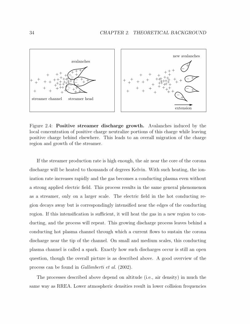
Though small, such avalanches can move enough charge to affect their surroundings.
This nonlinear feedback effect allows the production of “streamers,” self-sustaining
discharges continually fed by avalanches near their tip as shown in Figure 2.4. Es-
sentially, electric fields above Ek render air conducting. The conductivity leads to
a decay in the electric field in some regions, but intensification of the electric field
near the tip of the conducting region. This intensification allows the electric field to
remain above Ek over a small region, the so-called streamer head. The streamer head
constantly advances with the continual interplay of avalanche, field decay and field
intensification near the head at a velocity vs ' 106 m/s (for further detail, see Raizer ,
1997, p. 334–338).
Under conditions of sustained high voltage applied to an electrode, streamers are
continually produced and propagate away from the electrode resulting in a faint glow
around the tip of the electrode called corona discharge. Streamers propagate until
the electric field drops below a critical threshold value Ecr that depends on whether
the streamer is positively or negatively charged. For negatively charged streamers,
E−cr ' 1.25 MV/m, while for positively charged streamers E+cr ' 0.44 MV/m.
34 CHAPTER 2. THEORETICAL BACKGROUND
Figure 2.4: Positive streamer discharge growth. Avalanches induced by thelocal concentration of positive charge neutralize portions of this charge while leavingpositive charge behind elsewhere. This leads to an overall migration of the chargeregion and growth of the streamer.
If the streamer production rate is high enough, the air near the core of the corona
discharge will be heated to thousands of degrees Kelvin. With such heating, the ion-
ization rate increases rapidly and the gas becomes a conducting plasma even without
a strong applied electric field. This process results in the same general phenomenon
as a streamer, only on a larger scale. The electric field in the hot conducting re-
gion decays away but is correspondingly intensified near the edges of the conducting
region. If this intensification is sufficient, it will heat the gas in a new region to con-
ducting, and the process will repeat. This growing discharge process leaves behind a
conducting hot plasma channel through which a current flows to sustain the corona
discharge near the tip of the channel. On small and medium scales, this conducting
plasma channel is called a spark. Exactly how such discharges occur is still an open
question, though the overall picture is as described above. A good overview of the
process can be found in Gallimberti et al. (2002).
The processes described above depend on altitude (i.e., air density) in much the
same way as RREA. Lower atmospheric densities result in lower collision frequencies
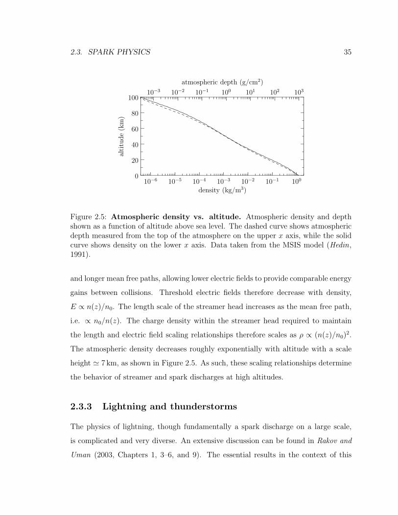
2.3. SPARK PHYSICS 35
0
20
40
60
80
100
alti
tude
(km
)
10−6 10−5 10−4 10−3 10−2 10−1 100
density (kg/m3)
10−3 10−2 10−1 100 101 102 103
atmospheric depth (g/cm2)
Figure 2.5: Atmospheric density vs. altitude. Atmospheric density and depthshown as a function of altitude above sea level. The dashed curve shows atmosphericdepth measured from the top of the atmosphere on the upper x axis, while the solidcurve shows density on the lower x axis. Data taken from the MSIS model (Hedin,1991).
and longer mean free paths, allowing lower electric fields to provide comparable energy
gains between collisions. Threshold electric fields therefore decrease with density,
E ∝ n(z)/n0. The length scale of the streamer head increases as the mean free path,
i.e. ∝ n0/n(z). The charge density within the streamer head required to maintain
the length and electric field scaling relationships therefore scales as ρ ∝ (n(z)/n0)2.
The atmospheric density decreases roughly exponentially with altitude with a scale
height ' 7 km, as shown in Figure 2.5. As such, these scaling relationships determine
the behavior of streamer and spark discharges at high altitudes.
2.3.3 Lightning and thunderstorms
The physics of lightning, though fundamentally a spark discharge on a large scale,
is complicated and very diverse. An extensive discussion can be found in Rakov and
Uman (2003, Chapters 1, 3–6, and 9). The essential results in the context of this
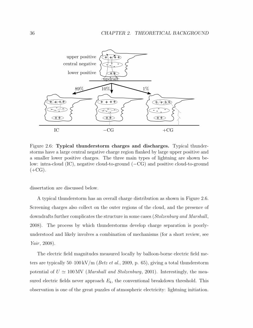
36 CHAPTER 2. THEORETICAL BACKGROUND
Figure 2.6: Typical thunderstorm charges and discharges. Typical thunder-storms have a large central negative charge region flanked by large upper positive anda smaller lower positive charges. The three main types of lightning are shown be-low: intra-cloud (IC), negative cloud-to-ground (−CG) and positive cloud-to-ground(+CG).
dissertation are discussed below.
A typical thunderstorm has an overall charge distribution as shown in Figure 2.6.
Screening charges also collect on the outer regions of the cloud, and the presence of
downdrafts further complicates the structure in some cases (Stolzenburg and Marshall ,
2008). The process by which thunderstorms develop charge separation is poorly-
understood and likely involves a combination of mechanisms (for a short review, see
Yair , 2008).
The electric field magnitudes measured locally by balloon-borne electric field me-
ters are typically 50–100 kV/m (Betz et al., 2009, p. 65), giving a total thunderstorm
potential of U ' 100 MV (Marshall and Stolzenburg , 2001). Interestingly, the mea-
sured electric fields never approach Ek, the conventional breakdown threshold. This
observation is one of the great puzzles of atmospheric electricity: lightning initiation.
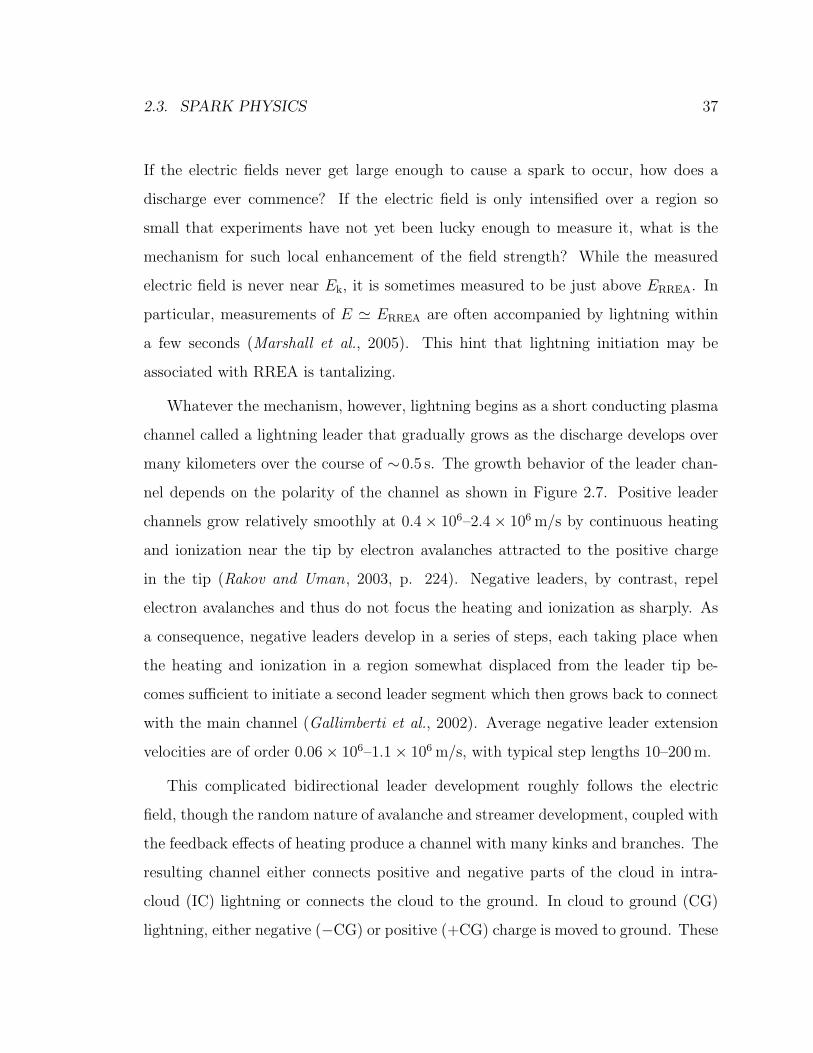
2.3. SPARK PHYSICS 37
If the electric fields never get large enough to cause a spark to occur, how does a
discharge ever commence? If the electric field is only intensified over a region so
small that experiments have not yet been lucky enough to measure it, what is the
mechanism for such local enhancement of the field strength? While the measured
electric field is never near Ek, it is sometimes measured to be just above ERREA. In
particular, measurements of E ' ERREA are often accompanied by lightning within
a few seconds (Marshall et al., 2005). This hint that lightning initiation may be
associated with RREA is tantalizing.
Whatever the mechanism, however, lightning begins as a short conducting plasma
channel called a lightning leader that gradually grows as the discharge develops over
many kilometers over the course of ∼0.5 s. The growth behavior of the leader chan-
nel depends on the polarity of the channel as shown in Figure 2.7. Positive leader
channels grow relatively smoothly at 0.4× 10⁶–2.4× 10⁶ m/s by continuous heating
and ionization near the tip by electron avalanches attracted to the positive charge
in the tip (Rakov and Uman, 2003, p. 224). Negative leaders, by contrast, repel
electron avalanches and thus do not focus the heating and ionization as sharply. As
a consequence, negative leaders develop in a series of steps, each taking place when
the heating and ionization in a region somewhat displaced from the leader tip be-
comes sufficient to initiate a second leader segment which then grows back to connect
with the main channel (Gallimberti et al., 2002). Average negative leader extension
velocities are of order 0.06× 10⁶–1.1× 10⁶ m/s, with typical step lengths 10–200 m.
This complicated bidirectional leader development roughly follows the electric
field, though the random nature of avalanche and streamer development, coupled with
the feedback effects of heating produce a channel with many kinks and branches. The
resulting channel either connects positive and negative parts of the cloud in intra-
cloud (IC) lightning or connects the cloud to the ground. In cloud to ground (CG)
lightning, either negative (−CG) or positive (+CG) charge is moved to ground. These
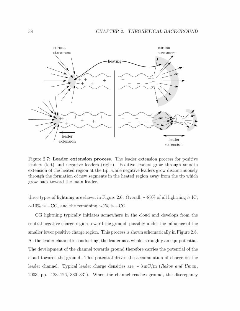
38 CHAPTER 2. THEORETICAL BACKGROUND
Figure 2.7: Leader extension process. The leader extension process for positiveleaders (left) and negative leaders (right). Positive leaders grow through smoothextension of the heated region at the tip, while negative leaders grow discontinuouslythrough the formation of new segments in the heated region away from the tip whichgrow back toward the main leader.
three types of lightning are shown in Figure 2.6. Overall, ∼89% of all lightning is IC,
∼10% is −CG, and the remaining ∼1% is +CG.
CG lightning typically initiates somewhere in the cloud and develops from the
central negative charge region toward the ground, possibly under the influence of the
smaller lower positive charge region. This process is shown schematically in Figure 2.8.
As the leader channel is conducting, the leader as a whole is roughly an equipotential.
The development of the channel towards ground therefore carries the potential of the
cloud towards the ground. This potential drives the accumulation of charge on the
leader channel. Typical leader charge densities are ∼ 3 mC/m (Rakov and Uman,
2003, pp. 123–126, 330–331). When the channel reaches ground, the discrepancy
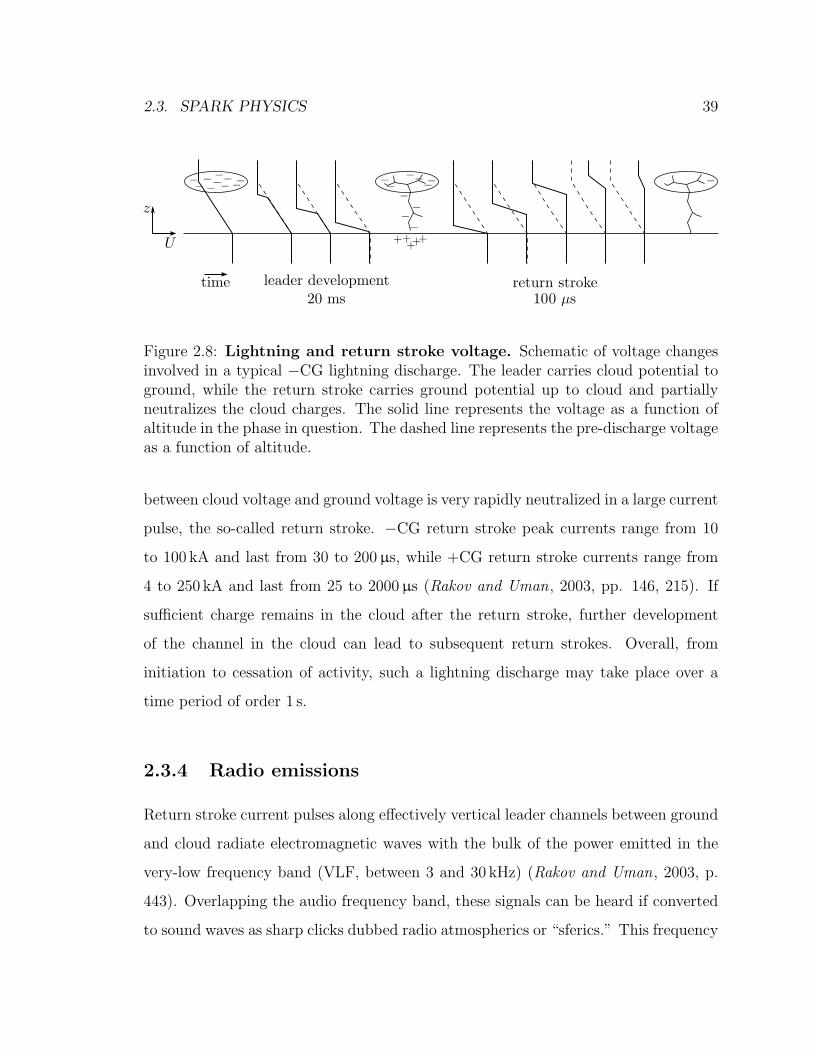
2.3. SPARK PHYSICS 39
Figure 2.8: Lightning and return stroke voltage. Schematic of voltage changesinvolved in a typical −CG lightning discharge. The leader carries cloud potential toground, while the return stroke carries ground potential up to cloud and partiallyneutralizes the cloud charges. The solid line represents the voltage as a function ofaltitude in the phase in question. The dashed line represents the pre-discharge voltageas a function of altitude.
between cloud voltage and ground voltage is very rapidly neutralized in a large current
pulse, the so-called return stroke. −CG return stroke peak currents range from 10
to 100 kA and last from 30 to 200 µs, while +CG return stroke currents range from
4 to 250 kA and last from 25 to 2000 µs (Rakov and Uman, 2003, pp. 146, 215). If
sufficient charge remains in the cloud after the return stroke, further development
of the channel in the cloud can lead to subsequent return strokes. Overall, from
initiation to cessation of activity, such a lightning discharge may take place over a
time period of order 1 s.
2.3.4 Radio emissions
Return stroke current pulses along effectively vertical leader channels between ground
and cloud radiate electromagnetic waves with the bulk of the power emitted in the
very-low frequency band (VLF, between 3 and 30 kHz) (Rakov and Uman, 2003, p.
443). Overlapping the audio frequency band, these signals can be heard if converted
to sound waves as sharp clicks dubbed radio atmospherics or “sferics.” This frequency
40 CHAPTER 2. THEORETICAL BACKGROUND
band is also efficiently reflected by both the ground and the ionosphere and is therefore
confined to and guided by the Earth-ionosphere waveguide. These signals can thus
be detected from great distances, up to 10 Mm or more.
Such VLF radio emissions allow for remote detection of lightning, a fact mentioned
in the context of TGF studies in Section 1.2.2. In particular, radio emissions can
be used to determine the location of the source lightning. A review of lightning
geolocation techniques can be found in Rakov and Uman (2003, pp. 555–587). The
direction from which a signal arrives at a receiver can be determined by comparing
the signals received by two orthogonal antennas (Wood and Inan, 2002). If the signal
is received at three or more receivers, advanced arrival time determination techniques
allow the location and time of the source lightning discharge to be determined very
accurately (Said , 2009). The shape and duration of the radio pulse received allows the
peak current and charge moment change parameters of the lightning to be determined
(Cummer and Inan, 2000; Wood , 2004).
IC lightning, by contrast, does not connect to the ground and therefore does not
show the rapid current pulses and voltage changes seen in return strokes. The current
structures in IC lightning are therefore largely driven by the development of the
channel into charge regions of varying density. Phenomena such as J- and K-processes
(measured electric field changes during a lightning discharge not associated with a
return stroke Rakov and Uman, 2003, pp. 183–188), and M-components (current
surges observed in lightning channels Rakov and Uman, 2003, pp. 177–182) are likely
due to such development and the resulting currents as charge densities on and near
the leader channel are rearranged.
As typical IC lightning does not have the characteristic vertical channel seen in CG
lightning, the lack of vertical currents prevents radio emissions from IC lightning from
efficiently driving modes of the Earth-ionosphere waveguide. IC lightning therefore
cannot typically be detected from large distances in VLF radio observations and is
2.3. SPARK PHYSICS 41
therefore relatively difficult to study. This difficulty, together with the fact that
IC lightning does not damage ground structures or start fires, has left study of IC
discharge a low priority.
This picture changed with the development of 3-dimensional lightning mapping
techniques such as those used by the New Mexico Tech Lightning Mapping Array
(LMA, see Rison et al., 1999). Such systems are limited to lightning no further than
a few hundred kilometers from the receivers, but observe each lightning discharge as
a sequence of high-frequency (HF, 60–66 MHz for the LMA) pulses, each associated
with small bursts of activity associated with extension of the leader channel. Such
HF pulses are emitted frequently by negative leaders due to the stepping process,
but also appear weakly for positive leaders. These HF pulses (discussed in detail in
Thomas et al., 2001) are detected at an array of receivers, and their arrival times are
used to triangulate the source location in three dimensions. The result is a map in
space and time of HF radio activity which allows the approximate path of the leader
channel in the cloud to be estimated. This window into IC activity can be used for
example to study lightning initiation (Betz et al., 2008), IC lightning currents, and
chemical effects (Betz et al., 2009, pp. 231–251).
The physics of lightning, though a complex process ranging from sub-millimeter
electron avalanches and streamers to multi-kilometer leader channels, can be summa-
rized as follows. Updrafts drive air currents which produce a charge structure as shown
in Figure 2.6. Some unknown mechanism subsequently initiates lightning. Lightning
then proceeds as the bidirectional development of a conducting leader channel which
allows charge from the thunderstorm to rearrange. If the leader reaches the ground
(CG lightning), the large and sudden voltage changes drive a powerful current (the
return stroke), which neutralizes charges along the channel and efficiently radiates
impulsive VLF radio waves that can be detected from great distances. If the leader
channel does not reach ground (IC lightning), current pulses are driven by channel
42 CHAPTER 2. THEORETICAL BACKGROUND
extension and the resulting rearrangements of charge. These discharge processes are
summarized in Table 2.1. How these processes may result in TGF production is the
subject of the next section.
2.4 TGF production theories
As discussed at the beginning of this chapter, TGFs involve high-energy photons
produced by bremsstrahlung. These bremsstrahlung photons come from energetic
electrons accelerated by electric fields. The observed coincidence with lightning sug-
gests that these electric fields are associated with lightning and thunderstorms. The
consideration of energetic electron and photon physics (Sections 2.1.1 and 2.1.2) and
their behavior in electric fields leads to predictions of the avalanche growth of pop-
ulations of energetic electrons (RREA), facilitating the production of large bursts of
bremsstrahlung photons. This outline of TGF physics is shown in Figure 2.9.
The main unknown in this picture is the mechanism of production of the elec-
tric field. Studies of thunderstorms and lightning do little more than suggest that
such fields might exist, leaving their behavior and magnitude unknown. To attempt
to provide a more complete picture, two main mechanisms have been proposed for
electric field production and subsequent TGF generation: the quasi-electrostatic and
electromagnetic pulse mechanisms.
2.4.1 Quasi-electrostatic mechanism
The quasi-electrostatic TGF production mechanism is a modernization of C. T.
R. Wilson’s observation that the electric field above a thundercloud decreases less
quickly than the atmospheric density, first discussed here in Section 1.1. The rapidly-
decreasing atmospheric density results in rapidly-decreasing threshold electric field
strengths, both for sparking as noted by Wilson and for RREA. This realization
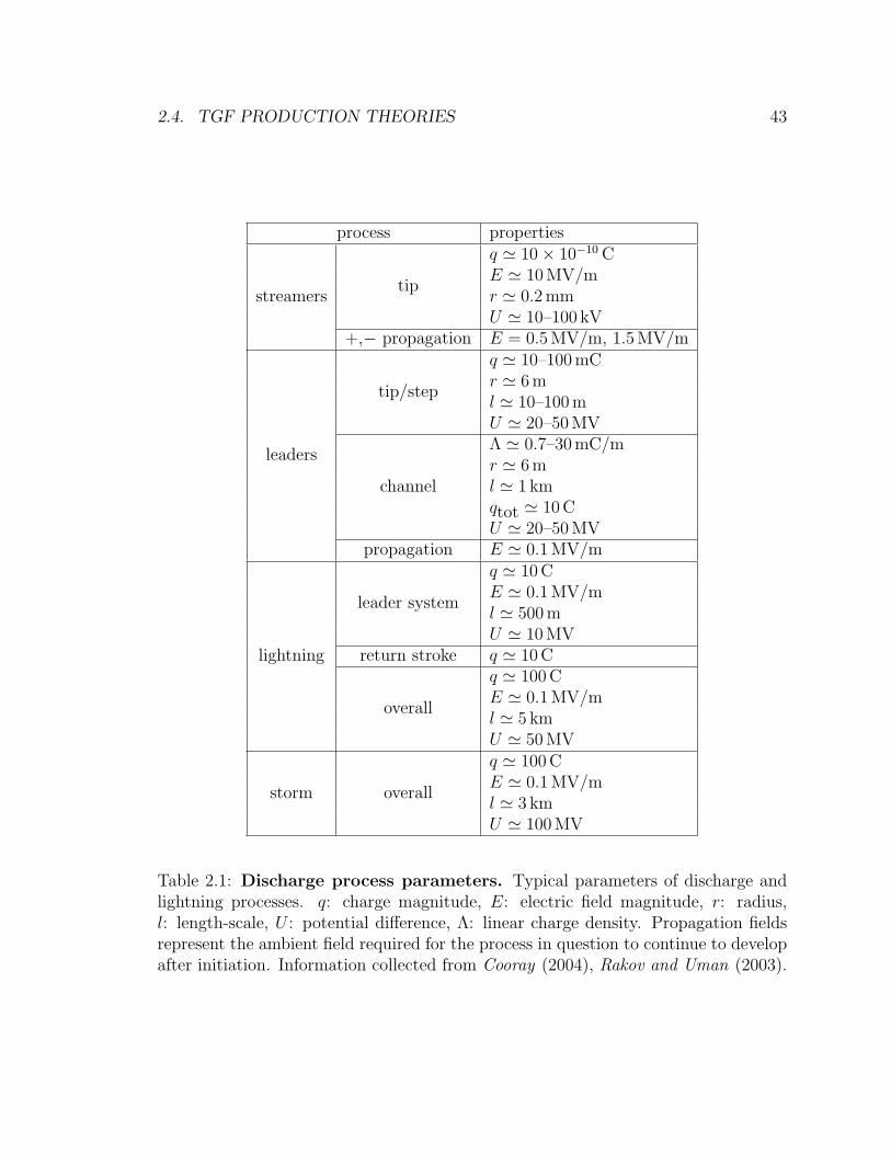
2.4. TGF PRODUCTION THEORIES 43
process properties
streamerstip
q ' 10× 10−10 CE ' 10 MV/mr ' 0.2 mmU ' 10–100 kV
+,− propagation E = 0.5 MV/m, 1.5 MV/m
leaders
tip/step
q ' 10–100 mCr ' 6 ml ' 10–100 mU ' 20–50 MV
channel
Λ ' 0.7–30 mC/mr ' 6 ml ' 1 kmqtot ' 10 CU ' 20–50 MV
propagation E ' 0.1 MV/m
lightning
leader system
q ' 10 CE ' 0.1 MV/ml ' 500 mU ' 10 MV
return stroke q ' 10 C
overall
q ' 100 CE ' 0.1 MV/ml ' 5 kmU ' 50 MV
storm overall
q ' 100 CE ' 0.1 MV/ml ' 3 kmU ' 100 MV
Table 2.1: Discharge process parameters. Typical parameters of discharge andlightning processes. q: charge magnitude, E: electric field magnitude, r: radius,l: length-scale, U : potential difference, Λ: linear charge density. Propagation fieldsrepresent the ambient field required for the process in question to continue to developafter initiation. Information collected from Cooray (2004), Rakov and Uman (2003).
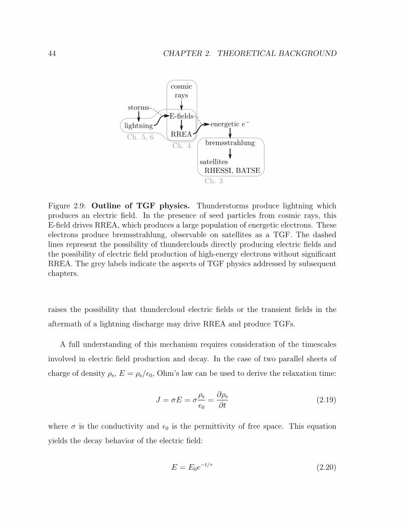
44 CHAPTER 2. THEORETICAL BACKGROUND
Figure 2.9: Outline of TGF physics. Thunderstorms produce lightning whichproduces an electric field. In the presence of seed particles from cosmic rays, thisE-field drives RREA, which produces a large population of energetic electrons. Theseelectrons produce bremsstrahlung, observable on satellites as a TGF. The dashedlines represent the possibility of thunderclouds directly producing electric fields andthe possibility of electric field production of high-energy electrons without significantRREA. The grey labels indicate the aspects of TGF physics addressed by subsequentchapters.
raises the possibility that thundercloud electric fields or the transient fields in the
aftermath of a lightning discharge may drive RREA and produce TGFs.
A full understanding of this mechanism requires consideration of the timescales
involved in electric field production and decay. In the case of two parallel sheets of
charge of density ρs, E = ρs/ε0, Ohm’s law can be used to derive the relaxation time:
J = σE = σρs
ε0=∂ρs
∂t(2.19)
where σ is the conductivity and ε0 is the permittivity of free space. This equation
yields the decay behavior of the electric field:
E = E0e−t/τ (2.20)
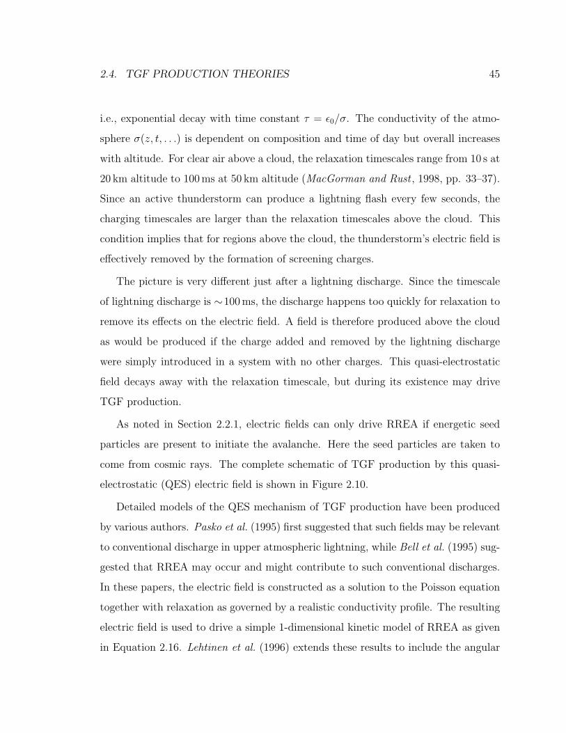
2.4. TGF PRODUCTION THEORIES 45
i.e., exponential decay with time constant τ = ε0/σ. The conductivity of the atmo-
sphere σ(z, t, . . .) is dependent on composition and time of day but overall increases
with altitude. For clear air above a cloud, the relaxation timescales range from 10 s at
20 km altitude to 100 ms at 50 km altitude (MacGorman and Rust , 1998, pp. 33–37).
Since an active thunderstorm can produce a lightning flash every few seconds, the
charging timescales are larger than the relaxation timescales above the cloud. This
condition implies that for regions above the cloud, the thunderstorm’s electric field is
effectively removed by the formation of screening charges.
The picture is very different just after a lightning discharge. Since the timescale
of lightning discharge is ∼100 ms, the discharge happens too quickly for relaxation to
remove its effects on the electric field. A field is therefore produced above the cloud
as would be produced if the charge added and removed by the lightning discharge
were simply introduced in a system with no other charges. This quasi-electrostatic
field decays away with the relaxation timescale, but during its existence may drive
TGF production.
As noted in Section 2.2.1, electric fields can only drive RREA if energetic seed
particles are present to initiate the avalanche. Here the seed particles are taken to
come from cosmic rays. The complete schematic of TGF production by this quasi-
electrostatic (QES) electric field is shown in Figure 2.10.
Detailed models of the QES mechanism of TGF production have been produced
by various authors. Pasko et al. (1995) first suggested that such fields may be relevant
to conventional discharge in upper atmospheric lightning, while Bell et al. (1995) sug-
gested that RREA may occur and might contribute to such conventional discharges.
In these papers, the electric field is constructed as a solution to the Poisson equation
together with relaxation as governed by a realistic conductivity profile. The resulting
electric field is used to drive a simple 1-dimensional kinetic model of RREA as given
in Equation 2.16. Lehtinen et al. (1996) extends these results to include the angular
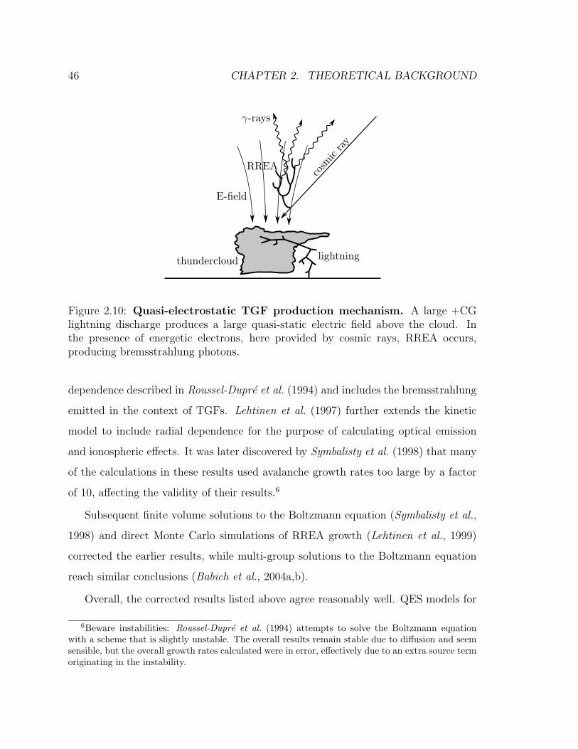
46 CHAPTER 2. THEORETICAL BACKGROUND
Figure 2.10: Quasi-electrostatic TGF production mechanism. A large +CGlightning discharge produces a large quasi-static electric field above the cloud. Inthe presence of energetic electrons, here provided by cosmic rays, RREA occurs,producing bremsstrahlung photons.
dependence described in Roussel-Dupre et al. (1994) and includes the bremsstrahlung
emitted in the context of TGFs. Lehtinen et al. (1997) further extends the kinetic
model to include radial dependence for the purpose of calculating optical emission
and ionospheric effects. It was later discovered by Symbalisty et al. (1998) that many
of the calculations in these results used avalanche growth rates too large by a factor
of 10, affecting the validity of their results.6
Subsequent finite volume solutions to the Boltzmann equation (Symbalisty et al.,
1998) and direct Monte Carlo simulations of RREA growth (Lehtinen et al., 1999)
corrected the earlier results, while multi-group solutions to the Boltzmann equation
reach similar conclusions (Babich et al., 2004a,b).
Overall, the corrected results listed above agree reasonably well. QES models for
6Beware instabilities: Roussel-Dupre et al. (1994) attempts to solve the Boltzmann equationwith a scheme that is slightly unstable. The overall results remain stable due to diffusion and seemsensible, but the overall growth rates calculated were in error, effectively due to an extra source termoriginating in the instability.
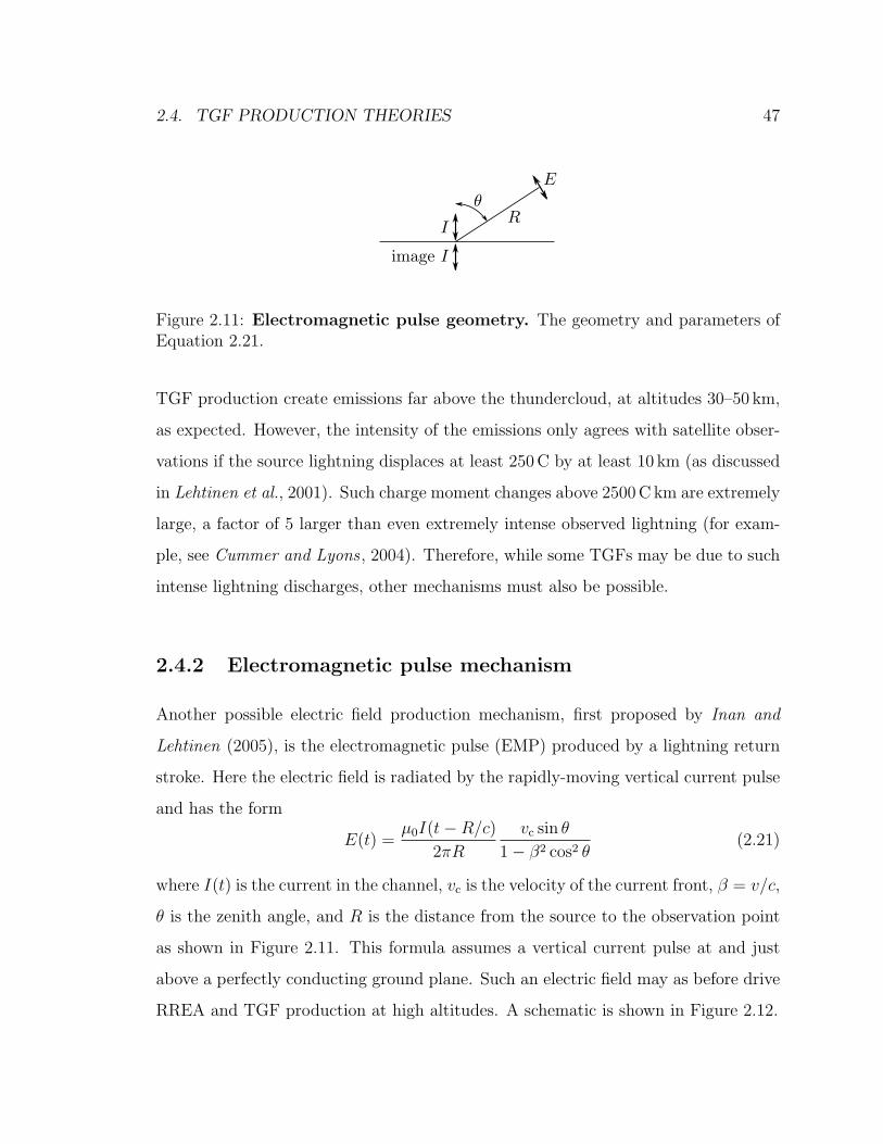
2.4. TGF PRODUCTION THEORIES 47
Figure 2.11: Electromagnetic pulse geometry. The geometry and parameters ofEquation 2.21.
TGF production create emissions far above the thundercloud, at altitudes 30–50 km,
as expected. However, the intensity of the emissions only agrees with satellite obser-
vations if the source lightning displaces at least 250 C by at least 10 km (as discussed
in Lehtinen et al., 2001). Such charge moment changes above 2500 C km are extremely
large, a factor of 5 larger than even extremely intense observed lightning (for exam-
ple, see Cummer and Lyons , 2004). Therefore, while some TGFs may be due to such
intense lightning discharges, other mechanisms must also be possible.
2.4.2 Electromagnetic pulse mechanism
Another possible electric field production mechanism, first proposed by Inan and
Lehtinen (2005), is the electromagnetic pulse (EMP) produced by a lightning return
stroke. Here the electric field is radiated by the rapidly-moving vertical current pulse
and has the form
E(t) =µ0I(t−R/c)
2πR
vc sin θ
1− β2 cos2 θ(2.21)
where I(t) is the current in the channel, vc is the velocity of the current front, β = v/c,
θ is the zenith angle, and R is the distance from the source to the observation point
as shown in Figure 2.11. This formula assumes a vertical current pulse at and just
above a perfectly conducting ground plane. Such an electric field may as before drive
RREA and TGF production at high altitudes. A schematic is shown in Figure 2.12.
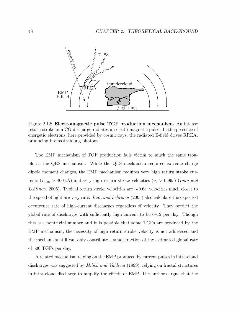
48 CHAPTER 2. THEORETICAL BACKGROUND
Figure 2.12: Electromagnetic pulse TGF production mechanism. An intensereturn stroke in a CG discharge radiates an electromagnetic pulse. In the presence ofenergetic electrons, here provided by cosmic rays, the radiated E-field drives RREA,producing bremsstrahlung photons.
The EMP mechanism of TGF production falls victim to much the same trou-
ble as the QES mechanism. While the QES mechanism required extreme charge
dipole moment changes, the EMP mechanism requires very high return stroke cur-
rents (Imax > 400 kA) and very high return stroke velocities (vc > 0.99c) (Inan and
Lehtinen, 2005). Typical return stroke velocities are ∼0.6c; velocities much closer to
the speed of light are very rare. Inan and Lehtinen (2005) also calculate the expected
occurrence rate of high-current discharges regardless of velocity. They predict the
global rate of discharges with sufficiently high current to be 6–12 per day. Though
this is a nontrivial number and it is possible that some TGFs are produced by the
EMP mechanism, the necessity of high return stroke velocity is not addressed and
the mechanism still can only contribute a small fraction of the estimated global rate
of 500 TGFs per day.
A related mechanism relying on the EMP produced by current pulses in intra-cloud
discharges was suggested by Milikh and Valdivia (1999), relying on fractal structures
in intra-cloud discharge to amplify the effects of EMP. The authors argue that the
2.4. TGF PRODUCTION THEORIES 49
fractal structures should result in amplification of the electric field by a factor of
∼5 by coherent summation of EMP emitted by different parts of the leader channel
and claim that their mechanism produces TGFs with current pulses >50 kA. While
intriguing, the mechanism does not account for any realistic current structure in the
lightning channel. Further, as described by Inan and Lehtinen (2005), Milikh and
Valdivia (1999) neglected a factor of 4π2 in one of their equations, a correction which
changes their current requirements from > 50 kA to > 2 MA, an unreasonably large
value.
2.4.3 Summary of TGF production mechanisms
The two main theories of TGF production by quasi-electrostatic (QES) and elec-
tromagnetic pulse (EMP) electric fields rely on extreme source lightning processes
to produce sufficiently strong electric fields. These mechanisms thus fall short of
explaining the observed TGFs.
The mechanisms have additional problems that are examined in more detail in
Chapters 3 and 4. First, both mechanisms predict emissions from high altitudes. As
discussed in Section 3.2.1, this prediction does not match the average observations
of TGFs, though this was not known when the mechanisms were constructed. The
QES and EMP mechanisms also involve various assumptions about the nature of
the source of RREA seed electrons. For instance, the EMP mechanism described in
Inan and Lehtinen (2005) assumes seed electrons produced by showers of secondary
particles from single primary cosmic rays with primary energies from 1016–1018 eV. As
discussed in Section 4.4, this assumption is not reasonable and the seed flux becomes
a limiting factor. These facts are explored in detail in the subsequent chapters.
Chapter 3
Constraints on source mechanisms
The terrestrial gamma-ray flash source poses a variety of questions. Fundamentally,
the source and behavior of the driving electric field are the key questions. More
practically, lower level questions are also posed, such as where the source is located
and what is its initial energy.
However, even these more direct questions cannot be immediately answered. All
that is known are the results of experiments, namely satellite observations of TGFs.
In the context of the summary of TGF physics given in Figure 2.9, the satellite
observations fall on the right end of the chain, while the most fundamental questions
about the physics of TGF production fall on the left. Examination of satellite data
to determine the properties of the TGF source therefore poses an inversion problem.
Given enough information toward the left half of Figure 2.9, the process can be
followed to the right to predict the satellite observations, but the satellite observations
themselves do not immediately allow inference of the nature of the processes at the
left in Figure 2.9.
This chapter describes a solution to this inversion problem by Monte Carlo sim-
ulation of the forward process. A source of photons is assumed and the resulting
50
3.1. MONTE CARLO SIMULATIONS 51
satellite observations are simulated. Comparison of the simulation results to the ac-
tual satellite data allows assessment of the assumed photon source. Results that do
not match the satellite observations can be used to rule out the particular assump-
tions used and thus constrain the TGF photon source. In particular, the results of
this chapter constrain the average TGF production altitude, energy, and the initial
angular distribution of TGF photons.
3.1 Monte Carlo simulations
The starting point for the simulations of TGF physics discussed in this chapter is taken
to be the emission of photons. This removes the electric field production mechanism
from consideration, greatly simplifying the inversion problem. Though this limits the
results to constraint of the photon source, such results are very useful as they can be
used to assess the validity of various photon production mechanisms.
As the goal is to study the photon source by comparing its effects to satellite data,
the assumed photon source should be taken to vary over as wide a range as possible.
Some overarching assumptions are necessary to limit the search, however. To render
the number of possible photon sources tractable, only point sources are considered.
This removes the complexity of the 3-dimensional shape of the photon source while
complicated shapes can be built by superposition of such point sources if required.
The altitude of the point source is taken to fall within 10–70 km. Sources lower than
10 km do not radiate significantly to satellite altitude, while the atmosphere above
70 km is too tenuous to produce a sufficient amount of bremsstrahlung.
Two initial photon energy spectra are considered. The first spectrum is that due
to thin-target bremsstrahlung produced by RREA electrons with energy spectrum
given in Lehtinen et al. (1999). The bremsstrahlung is generated by Monte Carlo
simulation with the GEANT4 software package (Agostinelli et al., 2003). This is the
52 CHAPTER 3. CONSTRAINTS ON SOURCE MECHANISMS
most realistic case, referred to as the bremsstrahlung initial spectrum hereafter. The
bremsstrahlung initial spectrum is similar to that used in Dwyer and Smith (2005) and
allows for comparison of results. The second spectrum is divorced from the mechanics
of photon emission and is the hardest spectrum producible by energetic electrons:
dN/dE ∝ 1/E , where 10 keV < E < 10 MeV. This limiting case is motivated by
the fact that the observed TGF spectrum is quite hard and is referred to as the
1/E case hereafter. Softer input spectra may be possible, but as the bremsstrahlung
initial spectrum is characteristic of energetic electrons driven by electric fields in air,
a substantially softer initial spectrum would likely require a mechanism inconsistent
with the general physical principles discussed in Chapter 2.
The initial directional distribution of the photons is chosen to be uniform with
zenith angle θ < θm. θm is taken to be either 1, 25, 45, or 90. θm = 1 corresponds
to the beam width of bremsstrahlung from unidirectional 35 MeV electrons, θm = 25
is characteristic of bremsstrahlung from RREA in a uniform electric field, and θm =
45 or 90 are broader beams that might result from nontrivial electric field structure.
The initial photons chosen from these distributions are then simulated as they
propagate in the Earth’s atmosphere. The Monte Carlo simulation tools used here
were written by Nikolai Lehtinen and are described in Lehtinen et al. (1999) and Lehti-
nen (2000). The atmosphere in which the photons propagate is taken to have con-
stant composition as a function of altitude with density taken from the MSIS model
(Hedin, 1991). Photoelectric absorption, Compton scattering, and pair production
are included with cross sections formulas similar to those given in Section 2.1.1. Pair
production is treated simplistically, with the produced positron immediately giving
rise to two oppositely-directed 0.511 MeV photons. As positron annihilation at rest
is more likely than annihilation in flight, this is a reasonable assumption.
This Monte Carlo code gives good results for the range of photon energies relevant
to TGFs. This can be validated by comparison to GEANT4, the industry-standard
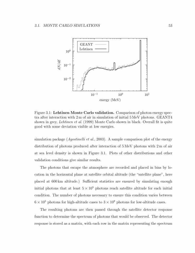
3.1. MONTE CARLO SIMULATIONS 53
Figure 3.1: Lehtinen Monte Carlo validation. Comparison of photon energy spec-tra after interaction with 2 m of air in simulation of initial 5 MeV photons. GEANT4shown in grey, Lehtinen et al. (1999) Monte Carlo shown in black. Overall fit is quitegood with some deviation visible at low energies.
simulation package (Agostinelli et al., 2003). A sample comparison plot of the energy
distribution of photons produced after interaction of 5 MeV photons with 2 m of air
at sea level density is shown in Figure 3.1. Plots of other distributions and other
validation conditions give similar results.
The photons that escape the atmosphere are recorded and placed in bins by lo-
cation in the horizontal plane at satellite orbital altitude (the “satellite plane”, here
placed at 600 km altitude.) Sufficient statistics are ensured by simulating enough
initial photons that at least 5× 10⁵ photons reach satellite altitude for each initial
condition. The number of photons necessary to ensure this condition varies between
6× 10⁵ photons for high-altitude cases to 3× 10⁹ photons for low-altitude cases.
The resulting photons are then passed through the satellite detector response
function to determine the spectrum of photons that would be observed. The detector
response is stored as a matrix, with each row in the matrix representing the spectrum
54 CHAPTER 3. CONSTRAINTS ON SOURCE MECHANISMS
that would be measured if a beam of photons of a particular energy was incident.
This analysis is carried out both for RHESSI and for BATSE. The detector response
matrices for BATSE are available in the Compton Observatory Science Support Cen-
ter (COSSC) data archive (http://cossc.gsfc.nasa.gov, discsc_drm files). The
detector response matrices for RHESSI were provided by Smith (2006). The result is
a set of possible observed spectra at various locations in the satellite plane.
The sensitivity of the satellite and the likelihood of detection of TGFs is then ac-
counted for by consideration of the relative intensities observed, similar to the method
used in Dwyer and Smith (2005). The most intense TGF observed by RHESSI is a
factor of 5 more intense than the least intense TGFs observable by RHESSI. BATSE
observes a similar ratio from most to least intense. Assuming that all TGFs have
similar inherent brightness and that all variation in TGF observations is therefore
due to observation of the TGF from various positions, the most intense TGF ob-
servations can be identified with the regions of the satellite plane where the spectra
are most intense. Likewise, the least intense observed TGFs can be identified with
the minimum sensitivity threshold for TGF detection. Those regions in the satellite
plane where the simulated spectra are less than one fifth as bright as the most intense
regions are therefore considered below the detection threshold and are discarded.
The remaining regions of the satellite plane, those with intensities within a factor
of 5 of the most intense regions, are considered as possible TGF observations. These
simulated observations contain spectra, relative intensity, and position information
ready for comparison to satellite observations. The simulated spectra vary with po-
sition but are averaged together for comparison with the average spectra seen by the
RHESSI and BATSE satellites. The number of photons simulated and the intensity
of the simulated spectrum is also tracked for calculation of the total energy input
necessary to produce simulated fluence that matches observations. The position as-
sociated with the simulated spectra and the resulting lateral displacement from the
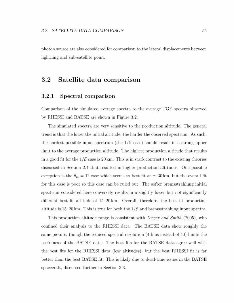
3.2. SATELLITE DATA COMPARISON 55
photon source are also considered for comparison to the lateral displacements between
lightning and sub-satellite point.
3.2 Satellite data comparison
3.2.1 Spectral comparison
Comparison of the simulated average spectra to the average TGF spectra observed
by RHESSI and BATSE are shown in Figure 3.2.
The simulated spectra are very sensitive to the production altitude. The general
trend is that the lower the initial altitude, the harder the observed spectrum. As such,
the hardest possible input spectrum (the 1/E case) should result in a strong upper
limit to the average production altitude. The highest production altitude that results
in a good fit for the 1/E case is 20 km. This is in stark contrast to the existing theories
discussed in Section 2.4 that resulted in higher production altitudes. One possible
exception is the θm = 1 case which seems to best fit at ' 30 km, but the overall fit
for this case is poor so this case can be ruled out. The softer bremsstrahlung initial
spectrum considered here conversely results in a slightly lower but not significantly
different best fit altitude of 15–20 km. Overall, therefore, the best fit production
altitude is 15–20 km. This is true for both the 1/E and bremsstrahlung input spectra.
This production altitude range is consistent with Dwyer and Smith (2005), who
confined their analysis to the RHESSI data. The BATSE data show roughly the
same picture, though the reduced spectral resolution (4 bins instead of 40) limits the
usefulness of the BATSE data. The best fits for the BATSE data agree well with
the best fits for the RHESSI data (low altitudes), but the best RHESSI fit is far
better than the best BATSE fit. This is likely due to dead-time issues in the BATSE
spacecraft, discussed further in Section 3.3.
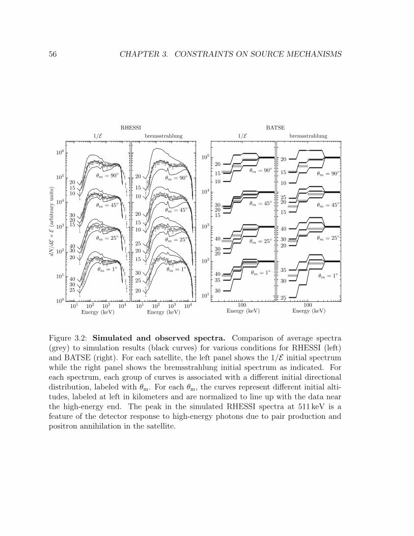
56 CHAPTER 3. CONSTRAINTS ON SOURCE MECHANISMS
Figure 3.2: Simulated and observed spectra. Comparison of average spectra(grey) to simulation results (black curves) for various conditions for RHESSI (left)and BATSE (right). For each satellite, the left panel shows the 1/E initial spectrumwhile the right panel shows the bremsstrahlung initial spectrum as indicated. Foreach spectrum, each group of curves is associated with a different initial directionaldistribution, labeled with θm. For each θm, the curves represent different initial alti-tudes, labeled at left in kilometers and are normalized to line up with the data nearthe high-energy end. The peak in the simulated RHESSI spectra at 511 keV is afeature of the detector response to high-energy photons due to pair production andpositron annihilation in the satellite.
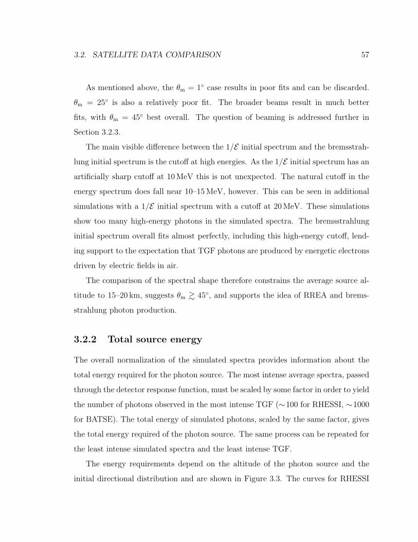
3.2. SATELLITE DATA COMPARISON 57
As mentioned above, the θm = 1 case results in poor fits and can be discarded.
θm = 25 is also a relatively poor fit. The broader beams result in much better
fits, with θm = 45 best overall. The question of beaming is addressed further in
Section 3.2.3.
The main visible difference between the 1/E initial spectrum and the bremsstrah-
lung initial spectrum is the cutoff at high energies. As the 1/E initial spectrum has an
artificially sharp cutoff at 10 MeV this is not unexpected. The natural cutoff in the
energy spectrum does fall near 10–15 MeV, however. This can be seen in additional
simulations with a 1/E initial spectrum with a cutoff at 20 MeV. These simulations
show too many high-energy photons in the simulated spectra. The bremsstrahlung
initial spectrum overall fits almost perfectly, including this high-energy cutoff, lend-
ing support to the expectation that TGF photons are produced by energetic electrons
driven by electric fields in air.
The comparison of the spectral shape therefore constrains the average source al-
titude to 15–20 km, suggests θm & 45, and supports the idea of RREA and brems-
strahlung photon production.
3.2.2 Total source energy
The overall normalization of the simulated spectra provides information about the
total energy required for the photon source. The most intense average spectra, passed
through the detector response function, must be scaled by some factor in order to yield
the number of photons observed in the most intense TGF (∼100 for RHESSI, ∼1000
for BATSE). The total energy of simulated photons, scaled by the same factor, gives
the total energy required of the photon source. The same process can be repeated for
the least intense simulated spectra and the least intense TGF.
The energy requirements depend on the altitude of the photon source and the
initial directional distribution and are shown in Figure 3.3. The curves for RHESSI
58 CHAPTER 3. CONSTRAINTS ON SOURCE MECHANISMS
Figure 3.3: Source energy requirements. The source energy required to matchsatellite observations for various conditions is shown by the grey and black lines. Thesolid grey bars and black lines represent the energy required to match the most andleast intense observed TGFs seen by the satellite as indicated in the key. Results areshown for different θm as indicated at right. The thin vertical lines and the dark greybox represent the best fit altitude from the spectral comparisons and the resultingenergy requirements. The results of the QES mechanisms due to Lehtinen et al.(1999) and Babich et al. (2004b) and the EMP mechanism due to Inan and Lehtinen(2005) are indicated.
and BATSE overall agree quite well, though they do not exactly overlap due to the
different detector response functions and the variability of the spectra with altitude
and directional distribution.
The energy and altitude of peak production for the existing mechanisms discussed
in Section 2.4 are also shown in this context. As mentioned above, though some
of the existing mechanisms can produce observable emissions, this only occurs for
unreasonably intense lightning and at altitudes higher than allowed by the spectral
consideration in Section 3.2.1. As the best fit spectra indicate a source altitude of
15–20 km and θm & 45, the total energy required is at least 1–10 kJ, corresponding to
a source population of 1015–1016 photons. Lower altitudes and broader beams require
even higher energies.
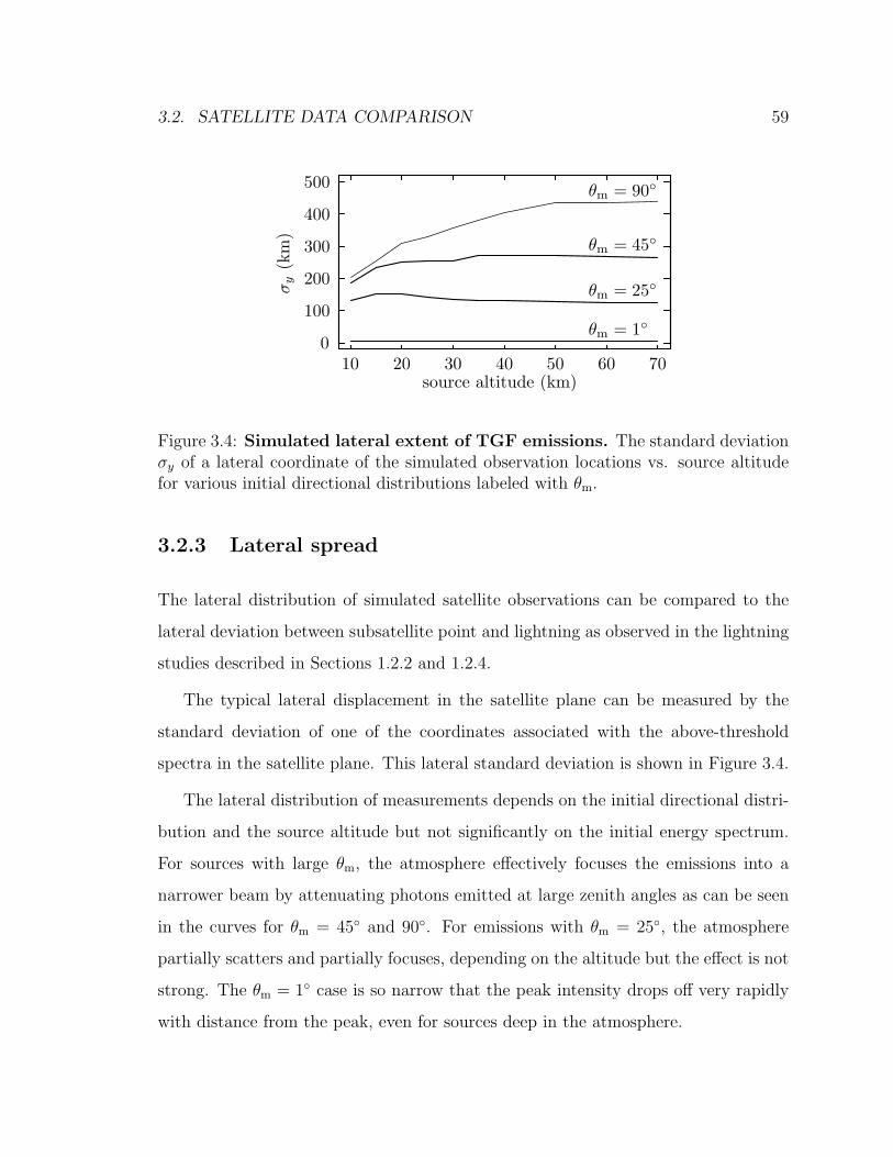
3.2. SATELLITE DATA COMPARISON 59
Figure 3.4: Simulated lateral extent of TGF emissions. The standard deviationσy of a lateral coordinate of the simulated observation locations vs. source altitudefor various initial directional distributions labeled with θm.
3.2.3 Lateral spread
The lateral distribution of simulated satellite observations can be compared to the
lateral deviation between subsatellite point and lightning as observed in the lightning
studies described in Sections 1.2.2 and 1.2.4.
The typical lateral displacement in the satellite plane can be measured by the
standard deviation of one of the coordinates associated with the above-threshold
spectra in the satellite plane. This lateral standard deviation is shown in Figure 3.4.
The lateral distribution of measurements depends on the initial directional distri-
bution and the source altitude but not significantly on the initial energy spectrum.
For sources with large θm, the atmosphere effectively focuses the emissions into a
narrower beam by attenuating photons emitted at large zenith angles as can be seen
in the curves for θm = 45 and 90. For emissions with θm = 25, the atmosphere
partially scatters and partially focuses, depending on the altitude but the effect is not
strong. The θm = 1 case is so narrow that the peak intensity drops off very rapidly
with distance from the peak, even for sources deep in the atmosphere.
60 CHAPTER 3. CONSTRAINTS ON SOURCE MECHANISMS
The typical subsatellite-lightning distances observed in radio observations of light-
ning coincident to TGFs are typically <300 km. For 15–20 km source altitudes as sug-
gested by the spectral studies, this is consistent with the θm & 45, also in agreement
with the spectral comparisons. Better statistics on subsatellite-lightning distance are
required to further address this issue.
3.3 Caveats
The studies described above are only as good as the assumptions used. The most
relevant assumptions are those that underlie the approximate treatment of the satel-
lite detection threshold. The key assumption is that all TGFs have the same source
properties and that all variation is due to the geometry of satellite observation. The
natural variation in TGF intensities is unknown, and it may be the case that an
observation of a TGF with relatively few photons is really an intrinsically dim TGF
observed at its brightest as opposed to an intrinsically bright TGF observed from a
relatively distant location. Studies involving nontrivial distributions in total initial
photon energy would help understand this effect.
Similarly, it is unlikely that TGFs are produced at only one altitude or with only
one effective θm. For instance, as mentioned in Section 2.4.2, it is possible that some
TGFs are produced by the EMP mechanism at high altitudes. While this is true, the
results here constrain the average TGF to be produced at relatively lower altitudes.
Studies involving nontrivial distributions in initial conditions may be useful, but for
the purposes of setting coarse constraints as is the goal here, the approach used should
be sufficient.
One important limitation to the BATSE spectrum and intensity analysis is dead-
time. The BATSE instrument was built with electronics that exhibit an energy-
dependent paralyzable dead-time that is shown to significantly affect BATSE TGF
3.4. SUMMARY OF TGF SOURCE PROPERTIES 61
observations by Grefenstette et al. (2008). This dead-time can be quite significant
(>50%) and contributes to an overall deficit in the total number of photons detected.
As suggested in Grefenstette et al. (2008), the dead-time also contributes to a relative
excess number of counts in the lowest-energy bin. As the most-energetic photons are
unlikely to have been significantly scattered and thus tend to have more direct paths
to the satellite and arrive sooner, the early photons at the peak brightness of the
TGF tend to have higher energies while late photons tend to have lower energies. As
a portion of the photons arriving during the peak brightness of the TGF are lost due
to dead-time, relatively more low-energy photons are observed as seen in Figure 4
of Grefenstette et al. (2008). Consideration of this fact helps to explain the poor
fits to BATSE spectra in Figure 3.2 but correspondingly limits the validity of the
comparison.
3.4 Summary of TGF source properties
These results show good agreement with the coarse ideas of TGF production described
in Chapter 2 if the photon source emits 1–10 kJ of energetic gamma-rays with a
bremsstrahlung spectrum at 15–20 km altitude and the photons are emitted in a broad
beam with effective half-angle θm & 45. These rough constraints are not dependent
on the details of any particular production mechanism, though the requirement of
photon emission by bremsstrahlung from electrons driven by electric fields is used to
determine feasible initial spectra. These constraints suggest that though the QES
and EMP production mechanisms may contribute some TGFs, the average behavior
indicates a new mechanism is required. The results described in this chapter are
available in the literature in Carlson et al. (2007).
Chapter 4
Electron avalanche seeding
The runaway relativistic electron avalanches suggested as crucial to TGF production
require seed runaway electrons to start the process, a fact first discussed in Sec-
tion 2.2.1. In the Earth’s atmosphere, these seed particles likely come from cosmic
rays. These statements raise more questions than they answer, however. For exam-
ple, do populations of such RREA seeds arrive all at once due to single relatively
energetic cosmic rays, or do they maintain a steady flux due to many lower-energy
cosmic rays? How does the seed population vary from one moment to the next?
Furthermore, how exactly do cosmic rays produce seeds? This chapter answers these
questions by consideration of cosmic ray physics and studies of the detailed physics
of RREA seeding.
4.1 Cosmic rays
Cosmic rays are the most energetic particles ever observed, with energies that some-
times exceed 1020 eV (Nagano and Watson, 2000), as much energy as a thrown base-
ball in a single atomic nucleus. Though little is known about their origins, results
from the Pierre Auger observatory suggest exotic astrophysical phenomena such as
62
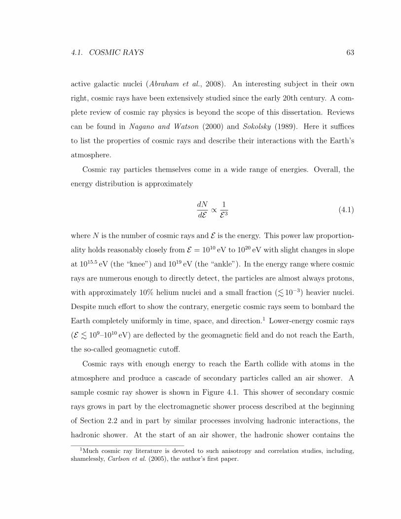
4.1. COSMIC RAYS 63
active galactic nuclei (Abraham et al., 2008). An interesting subject in their own
right, cosmic rays have been extensively studied since the early 20th century. A com-
plete review of cosmic ray physics is beyond the scope of this dissertation. Reviews
can be found in Nagano and Watson (2000) and Sokolsky (1989). Here it suffices
to list the properties of cosmic rays and describe their interactions with the Earth’s
atmosphere.
Cosmic ray particles themselves come in a wide range of energies. Overall, the
energy distribution is approximately
dN
dE ∝1
E3(4.1)
where N is the number of cosmic rays and E is the energy. This power law proportion-
ality holds reasonably closely from E = 1010 eV to 1020 eV with slight changes in slope
at 1015.5 eV (the “knee”) and 1019 eV (the “ankle”). In the energy range where cosmic
rays are numerous enough to directly detect, the particles are almost always protons,
with approximately 10% helium nuclei and a small fraction (. 10−3) heavier nuclei.
Despite much effort to show the contrary, energetic cosmic rays seem to bombard the
Earth completely uniformly in time, space, and direction.1 Lower-energy cosmic rays
(E . 109–1010 eV) are deflected by the geomagnetic field and do not reach the Earth,
the so-called geomagnetic cutoff.
Cosmic rays with enough energy to reach the Earth collide with atoms in the
atmosphere and produce a cascade of secondary particles called an air shower. A
sample cosmic ray shower is shown in Figure 4.1. This shower of secondary cosmic
rays grows in part by the electromagnetic shower process described at the beginning
of Section 2.2 and in part by similar processes involving hadronic interactions, the
hadronic shower. At the start of an air shower, the hadronic shower contains the
1Much cosmic ray literature is devoted to such anisotropy and correlation studies, including,shamelessly, Carlson et al. (2005), the author’s first paper.
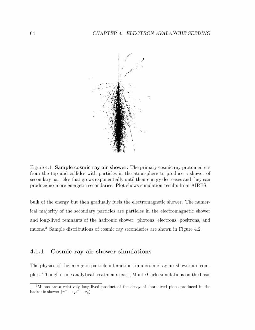
64 CHAPTER 4. ELECTRON AVALANCHE SEEDING
Figure 4.1: Sample cosmic ray air shower. The primary cosmic ray proton entersfrom the top and collides with particles in the atmosphere to produce a shower ofsecondary particles that grows exponentially until their energy decreases and they canproduce no more energetic secondaries. Plot shows simulation results from AIRES.
bulk of the energy but then gradually fuels the electromagnetic shower. The numer-
ical majority of the secondary particles are particles in the electromagnetic shower
and long-lived remnants of the hadronic shower: photons, electrons, positrons, and
muons.2 Sample distributions of cosmic ray secondaries are shown in Figure 4.2.
4.1.1 Cosmic ray air shower simulations
The physics of the energetic particle interactions in a cosmic ray air shower are com-
plex. Though crude analytical treatments exist, Monte Carlo simulations on the basis
2Muons are a relatively long-lived product of the decay of short-lived pions produced in thehadronic shower (π− → µ− + νµ).
4.1. COSMIC RAYS 65
0 10 20 30z, km
100
101
102
103
104
105
N(z
)(t
otal
par
ticl
es)
γe−
e+
µ−
y
x
5 kmy
x
y
x
y
x
Figure 4.2: Sample air shower secondary distributions. The number of photons,electrons, positrons, and muons is shown as a function of altitude in the main panel.Sample secondary particle lateral position distributions are shown above on a ±10 kmscale for 4, 11, 19, and 26 km altitudes. Data shown are AIRES simulation results foran air shower produced by a 1013 eV proton incident on the Earth’s atmosphere witha zenith angle θ ' 70 (cos θ = 0.35).
of descriptions of individual particle interactions are commonly used. There is unfor-
tunately some uncertainty in the models used to drive such Monte Carlo calculations,
especially in the hadronic shower, but overall it is well-accepted that such models
agree well with observations.
The simulations described in this chapter use the AIRES software package (Sci-
utto, 2002). AIRES is an advanced cosmic ray air shower simulation tool developed
by the Universidad Nacional de La Plata in Argentina. The version of AIRES used
here uses SIBYLL (a minijet model of hadronic processes) for simulation of hadronic
interactions, though AIRES also includes QGSJET and QGSJET-II (quark-gluon
string models.)
As cosmic ray air showers often contain too many secondary particles to feasibly
run simulations, AIRES implements a “thinning” algorithm whereby some low-energy
products of an interaction are ignored and the remaining low-energy products are
66 CHAPTER 4. ELECTRON AVALANCHE SEEDING
propagated as usual but with increased statistical weight. Fortunately, as discussed
later in this section, the highest-energy cosmic ray air showers for which computation
is prohibitively slow are not required here, so all simulation results reported are “un-
thinned.”
4.1.2 Overall cosmic ray secondary distributions
From the perspective of seeding RREA, the interesting question is what are the
distributions of cosmic ray secondaries in the electric field region? This reduces to
a determination of what cosmic ray primary particles are relevant, the properties of
these primary particles, and the properties of the secondary particles they contribute.
The starting point, however, is to consider a region of interest. The electric fields
relevant to TGF production must be roughly vertical and cover a large potential
difference and therefore must have significant vertical extent. The horizontal extent
is in principle unconstrained but here is assumed to be the same as the vertical extent.
The regions of interest considered are therefore spheres with radius chosen to range
from 100 m to 3 km. Also relevant is the timescale over which the electric field exists.
The light travel time over the region of interest is used here to focus on the initiation
of the avalanche before significant growth occurs. These regions of interest are taken
to fall at altitudes from 0 to 30 km, including the range of TGF production altitudes
allowed by the constraints discussed in Chapter 3.
The energies of cosmic ray primaries relevant to these regions of interest can then
be determined. The largest cross sectional area and timescale under consideration
are 28× 106 m2 and 10 µs. As the flux of cosmic rays with energies above 1015 eV
is ' 1 m−2 year−1, the expected number of such cosmic rays incident on the largest
region of interest within the timescale in question is '10−5. This therefore represents
a reasonable upper limit on the highest energy cosmic ray primary expected to be
relevant to the regions of interest considered. As mentioned above, cosmic rays with
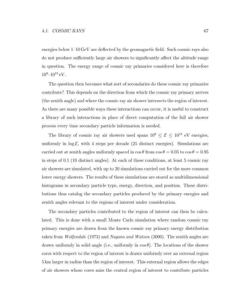
4.1. COSMIC RAYS 67
energies below 1–10 GeV are deflected by the geomagnetic field. Such cosmic rays also
do not produce sufficiently large air showers to significantly affect the altitude range
in question. The energy range of cosmic ray primaries considered here is therefore
109–1015 eV.
The question then becomes what sort of secondaries do these cosmic ray primaries
contribute? This depends on the direction from which the cosmic ray primary arrives
(the zenith angle) and where the cosmic ray air shower intersects the region of interest.
As there are many possible ways these interactions can occur, it is useful to construct
a library of such interactions in place of direct computation of the full air shower
process every time secondary particle information is needed.
The library of cosmic ray air showers used spans 109 ≤ E ≤ 1015 eV energies,
uniformly in log E , with 4 steps per decade (25 distinct energies). Simulations are
carried out at zenith angles uniformly spaced in cos θ from cos θ = 0.05 to cos θ = 0.95
in steps of 0.1 (10 distinct angles). At each of these conditions, at least 5 cosmic ray
air showers are simulated, with up to 20 simulations carried out for the more common
lower energy showers. The results of these simulations are stored as multidimensional
histograms in secondary particle type, energy, direction, and position. These distri-
butions thus catalog the secondary particles produced by the primary energies and
zenith angles relevant to the regions of interest under consideration.
The secondary particles contributed to the region of interest can then be calcu-
lated. This is done with a small Monte Carlo simulation where random cosmic ray
primary energies are drawn from the known cosmic ray primary energy distribution
taken from Wolfendale (1973) and Nagano and Watson (2000). The zenith angles are
drawn uniformly in solid angle (i.e., uniformly in cos θ). The locations of the shower
cores with respect to the region of interest is drawn uniformly over an external region
5 km larger in radius than the region of interest. This external region allows the edges
of air showers whose cores miss the central region of interest to contribute particles
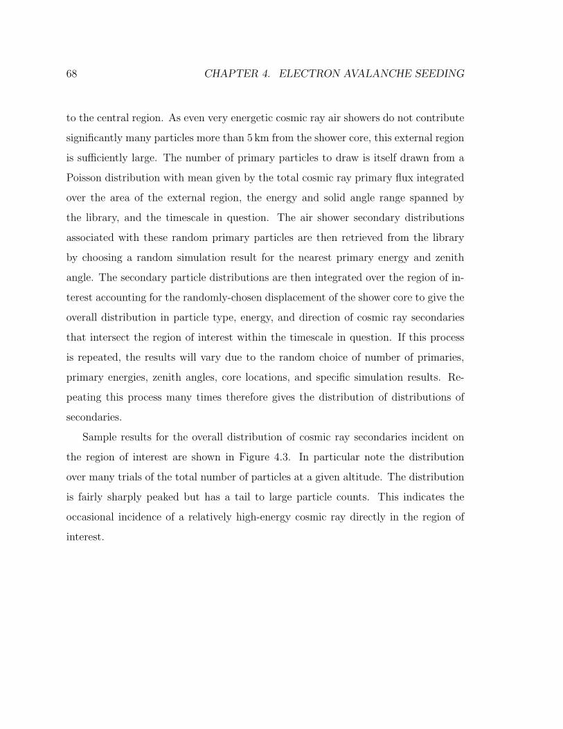
68 CHAPTER 4. ELECTRON AVALANCHE SEEDING
to the central region. As even very energetic cosmic ray air showers do not contribute
significantly many particles more than 5 km from the shower core, this external region
is sufficiently large. The number of primary particles to draw is itself drawn from a
Poisson distribution with mean given by the total cosmic ray primary flux integrated
over the area of the external region, the energy and solid angle range spanned by
the library, and the timescale in question. The air shower secondary distributions
associated with these random primary particles are then retrieved from the library
by choosing a random simulation result for the nearest primary energy and zenith
angle. The secondary particle distributions are then integrated over the region of in-
terest accounting for the randomly-chosen displacement of the shower core to give the
overall distribution in particle type, energy, and direction of cosmic ray secondaries
that intersect the region of interest within the timescale in question. If this process
is repeated, the results will vary due to the random choice of number of primaries,
primary energies, zenith angles, core locations, and specific simulation results. Re-
peating this process many times therefore gives the distribution of distributions of
secondaries.
Sample results for the overall distribution of cosmic ray secondaries incident on
the region of interest are shown in Figure 4.3. In particular note the distribution
over many trials of the total number of particles at a given altitude. The distribution
is fairly sharply peaked but has a tail to large particle counts. This indicates the
occasional incidence of a relatively high-energy cosmic ray directly in the region of
interest.
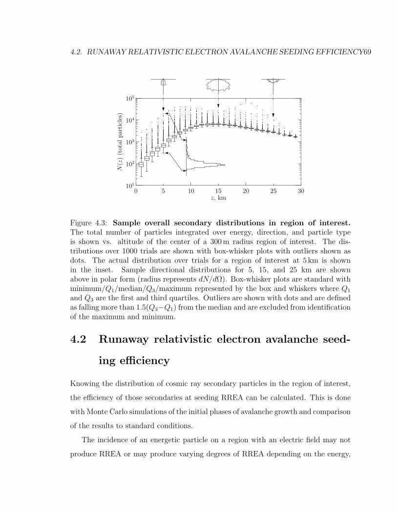
4.2. RUNAWAY RELATIVISTIC ELECTRON AVALANCHE SEEDING EFFICIENCY69
Figure 4.3: Sample overall secondary distributions in region of interest.The total number of particles integrated over energy, direction, and particle typeis shown vs. altitude of the center of a 300 m radius region of interest. The dis-tributions over 1000 trials are shown with box-whisker plots with outliers shown asdots. The actual distribution over trials for a region of interest at 5 km is shownin the inset. Sample directional distributions for 5, 15, and 25 km are shownabove in polar form (radius represents dN/dΩ). Box-whisker plots are standard withminimum/Q1/median/Q3/maximum represented by the box and whiskers where Q1
and Q3 are the first and third quartiles. Outliers are shown with dots and are definedas falling more than 1.5(Q3−Q1) from the median and are excluded from identificationof the maximum and minimum.
4.2 Runaway relativistic electron avalanche seed-
ing efficiency
Knowing the distribution of cosmic ray secondary particles in the region of interest,
the efficiency of those secondaries at seeding RREA can be calculated. This is done
with Monte Carlo simulations of the initial phases of avalanche growth and comparison
of the results to standard conditions.
The incidence of an energetic particle on a region with an electric field may not
produce RREA or may produce varying degrees of RREA depending on the energy,
70 CHAPTER 4. ELECTRON AVALANCHE SEEDING
direction, and type of the incoming particle. For instance, it is reasonable to expect
that energetic photons are not as good at seeding RREA as energetic electrons, and
that electrons moving in the direction of avalanche motion are better than electrons
moving opposite the avalanche.
These effects can be assessed by Monte Carlo simulation with the GEANT4 pack-
age (Agostinelli et al., 2003). In order to focus only on the seeding process without
losing information in the details of avalanche growth, specific time limits are imposed
on the simulations. The incident particle (the putative cosmic ray secondary) is only
simulated for 100 ns. This allows the incident particle enough time to interact and
produce energetic secondaries but limits other effects such as energy gain or loss in
the electric field. To allow for a standard small amount of avalanche growth, the
energetic secondary particles produced by the incident particle, together with any
other secondary particles produced, are tracked for up to 20 ns after the parent inci-
dent particle interaction. The particles are injected into an electric field 1.5 times the
RREA threshold field (E = 1.5ERREA). Sample electron production results of this
process are shown in Figure 4.4.
The total number of electrons that reach the end of their allowed lifetime is taken
to be a measure of the efficiency of RREA seeding of the incident particle. How-
ever, this number of electrons bears little physical insight as it depends on the time
limits used and thus must be compared to the number of electrons produced under
standard conditions to extract the relative seeding efficiency. The “standard” seed
particle is a typical avalanche particle: a 1 MeV electron (near the energy for min-
imum frictional losses) traveling in the direction of avalanche growth. The number
of electrons produced by this particle under the conditions of the simulation can be
used as a normalization to convert other seed conditions to the effective number of
1 MeV electrons moving with the avalanche, i.e. the effective number of RREA seed
particles.
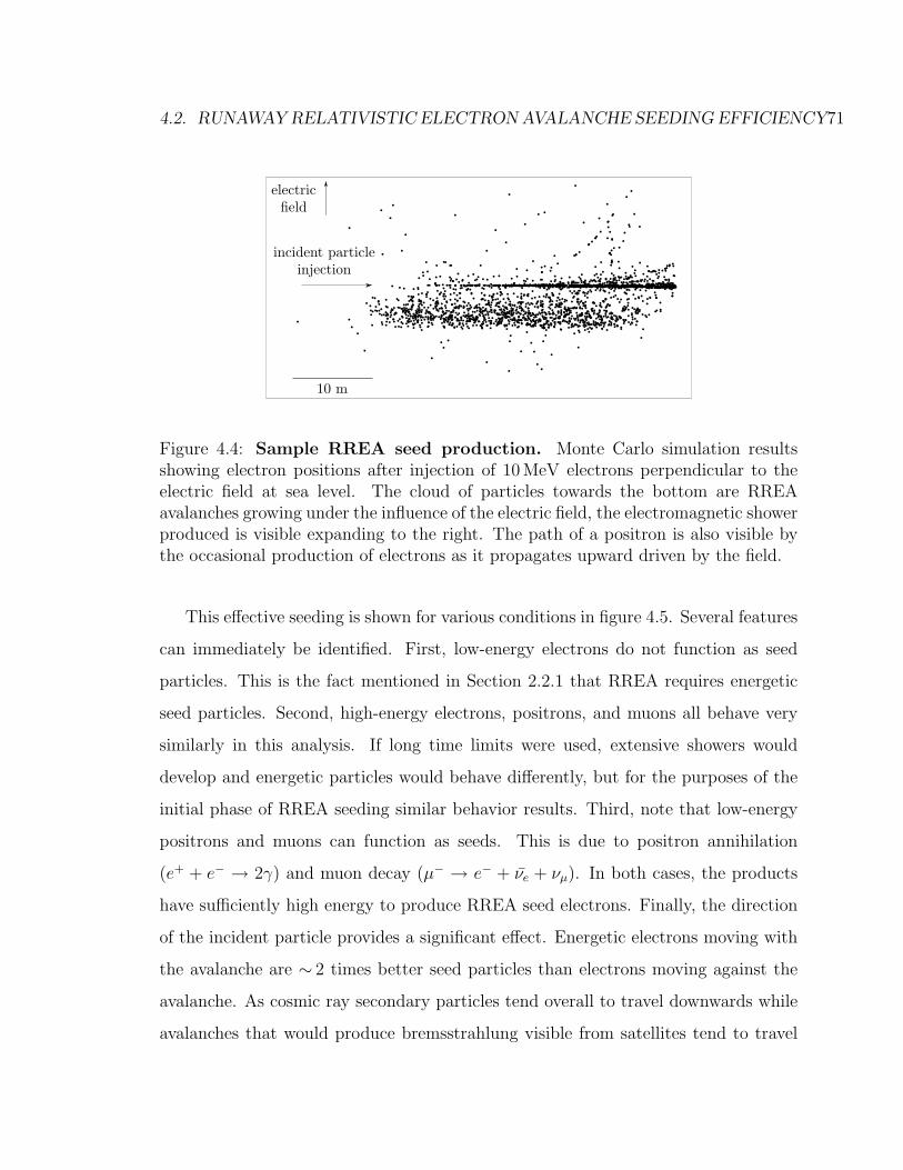
4.2. RUNAWAY RELATIVISTIC ELECTRON AVALANCHE SEEDING EFFICIENCY71
Figure 4.4: Sample RREA seed production. Monte Carlo simulation resultsshowing electron positions after injection of 10 MeV electrons perpendicular to theelectric field at sea level. The cloud of particles towards the bottom are RREAavalanches growing under the influence of the electric field, the electromagnetic showerproduced is visible expanding to the right. The path of a positron is also visible bythe occasional production of electrons as it propagates upward driven by the field.
This effective seeding is shown for various conditions in figure 4.5. Several features
can immediately be identified. First, low-energy electrons do not function as seed
particles. This is the fact mentioned in Section 2.2.1 that RREA requires energetic
seed particles. Second, high-energy electrons, positrons, and muons all behave very
similarly in this analysis. If long time limits were used, extensive showers would
develop and energetic particles would behave differently, but for the purposes of the
initial phase of RREA seeding similar behavior results. Third, note that low-energy
positrons and muons can function as seeds. This is due to positron annihilation
(e+ + e− → 2γ) and muon decay (µ− → e− + νe + νµ). In both cases, the products
have sufficiently high energy to produce RREA seed electrons. Finally, the direction
of the incident particle provides a significant effect. Energetic electrons moving with
the avalanche are ∼ 2 times better seed particles than electrons moving against the
avalanche. As cosmic ray secondary particles tend overall to travel downwards while
avalanches that would produce bremsstrahlung visible from satellites tend to travel
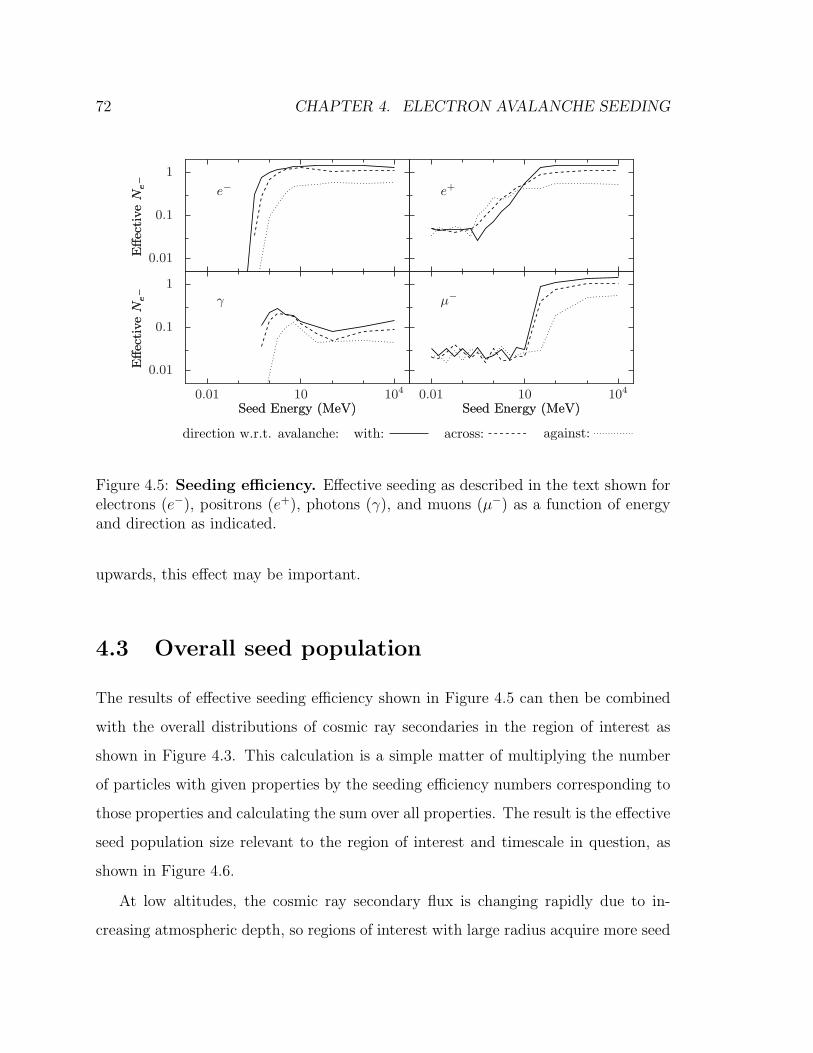
72 CHAPTER 4. ELECTRON AVALANCHE SEEDING
Figure 4.5: Seeding efficiency. Effective seeding as described in the text shown forelectrons (e−), positrons (e+), photons (γ), and muons (µ−) as a function of energyand direction as indicated.
upwards, this effect may be important.
4.3 Overall seed population
The results of effective seeding efficiency shown in Figure 4.5 can then be combined
with the overall distributions of cosmic ray secondaries in the region of interest as
shown in Figure 4.3. This calculation is a simple matter of multiplying the number
of particles with given properties by the seeding efficiency numbers corresponding to
those properties and calculating the sum over all properties. The result is the effective
seed population size relevant to the region of interest and timescale in question, as
shown in Figure 4.6.
At low altitudes, the cosmic ray secondary flux is changing rapidly due to in-
creasing atmospheric depth, so regions of interest with large radius acquire more seed
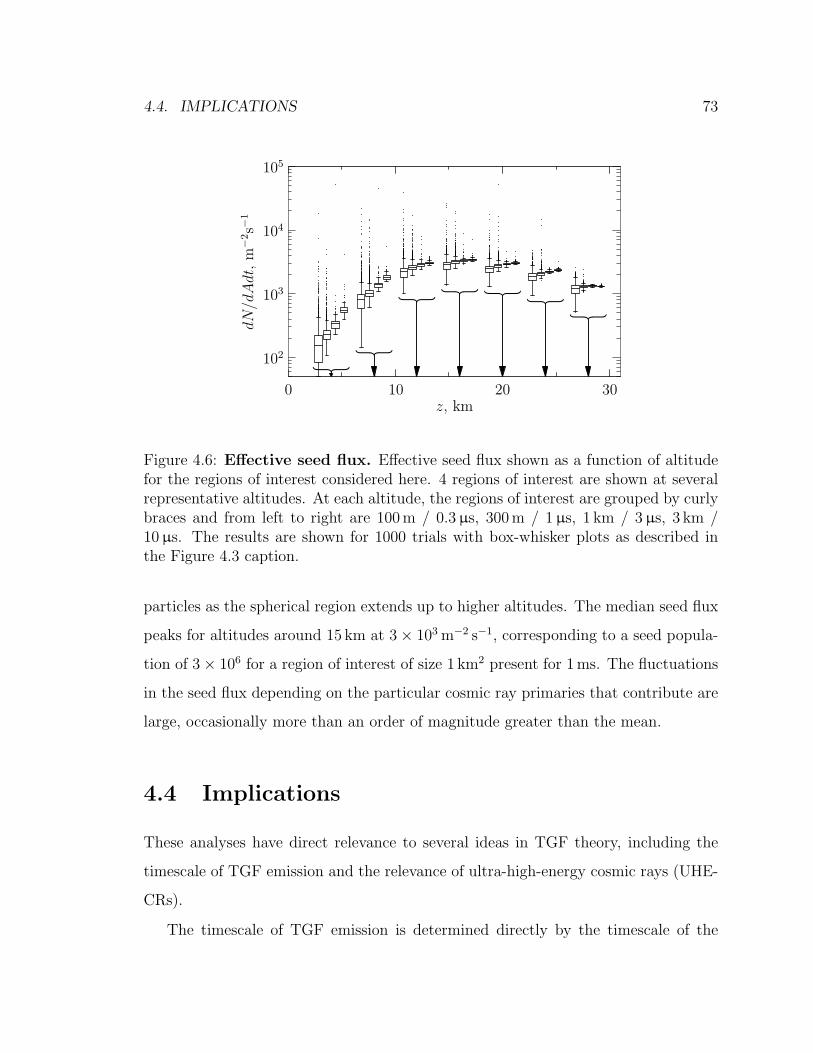
4.4. IMPLICATIONS 73
Figure 4.6: Effective seed flux. Effective seed flux shown as a function of altitudefor the regions of interest considered here. 4 regions of interest are shown at severalrepresentative altitudes. At each altitude, the regions of interest are grouped by curlybraces and from left to right are 100 m / 0.3 µs, 300 m / 1 µs, 1 km / 3 µs, 3 km /10 µs. The results are shown for 1000 trials with box-whisker plots as described inthe Figure 4.3 caption.
particles as the spherical region extends up to higher altitudes. The median seed flux
peaks for altitudes around 15 km at 3× 10³ m−2 s−1, corresponding to a seed popula-
tion of 3× 10⁶ for a region of interest of size 1 km2 present for 1 ms. The fluctuations
in the seed flux depending on the particular cosmic ray primaries that contribute are
large, occasionally more than an order of magnitude greater than the mean.
4.4 Implications
These analyses have direct relevance to several ideas in TGF theory, including the
timescale of TGF emission and the relevance of ultra-high-energy cosmic rays (UHE-
CRs).
The timescale of TGF emission is determined directly by the timescale of the
74 CHAPTER 4. ELECTRON AVALANCHE SEEDING
energetic electron population that emits the TGF via bremsstrahlung. The median
seed flux numbers show that seed particles are always present, even for small regions
of interest in short intervals of time. For example, at 15 km altitude, the 100 m radius
region of interest receives approximately 104 effective seed particles every 100 µs.
Essentially, as soon as the electric field exists, seed particles are present and RREA
will occur. The timescale of RREA therefore tracks the timescale of the electric field,
and if RREA growth alone is sufficient to produce detectable emissions, the TGF
timescale and the electric field timescale should be similar.
The relevance of ultra-high-energy cosmic rays (UHECRs) to RREA seeding is
contained in this analysis in the size of the fluctuations in the effective seed flux.
As the flux of UHECR primary particles is very low (integral flux above 1015 eV is
less than 1 m−2 year−1), the electric field must cover a large region if it is to catch a
UHECR and the large numbers of secondary particles it produces. However, exam-
ination of Figure 4.6 shows that as the region of interest gets larger, the size of the
fluctuations decreases. This is due to the increase in the number of lower-energy cos-
mic rays that intersect the region of interest as the area increases. In essence, though
large areas are more likely to catch UHECRs, the increased flux of UHECRs is out-
weighed by the increased flux of lower-energy cosmic rays such that the fluctuations
are damped out. This implies that UHECRs are not relevant in the context of seeding
RREA, and that the assumptions made in particular by Gurevich of single UHECR
air showers serving as seed particles are not valid without justification3 (Gurevich
and Zybin, 2004; Gurevich et al., 2004; Gurevich et al., 2002, 2004b, 2003). A similar
conclusion is reached by Dwyer (2007) by consideration of relativistic feedback limits
on the size of the electric field region, a topic discussed in more detail in Section 5.5.
3Selection effects where fluctuations so rare as to be completely negligible in this analysis nev-ertheless dominate the observable behavior may be relevant, but such effects are not consideredin existing mechanisms. These results indicate that claims of such behavior require very carefulconsideration.
4.4. IMPLICATIONS 75
In summary, initial RREA seed particles originate from cosmic rays, with the
majority of seed particles contributed by a large population of relatively low-energy
cosmic rays. The median seed flux is nontrivial, capable of seeding RREA whenever
a sufficiently-large electric field is present. The fluctuations in this median seed flux
are large, but not large enough to allow assumption of seed production by single
ultra-high-energy cosmic ray air showers. The results described in this chapter are
available in the literature in Carlson et al. (2008).
Chapter 5
Lightning and TGF production
The results derived in Chapters 3 and 4 pose a contradiction. The constraints on
source altitude and total photon source energy from Sections 3.2.1 and 3.2.2 indicate
a source of 1016 photons. Simulations of bremsstrahlung photon production such as
those executed with GEANT4 to construct the RREA initial spectrum used in Chap-
ter 3 indicate that production of such a population of photons requires a population
of electrons ∼10 times larger, i.e., 1017 total energetic electrons.
The largest seed population justifiable on the basis of the results in Chapter 4 is
∼ 107. A population of 1017 energetic electrons as produced by RREA from a seed
population of 107 electrons therefore requires a RREA avalanche growth factor of
M' 1010.
Equation 2.17, reproduced here without the parameter uncertainties, can be used
to calculate the RREA avalanche growth factor M:
λ(E) =7300 kV
E − 276 kV/m(5.1)
M = expL
λ(E)(5.2)
= exp
[L
(E − 276 kV/m
7300 kV
)](5.3)
76
77
= exp
(U − L276 kV/m
7300 kV
)(5.4)
Mmax = exp
(U
7300 kV
)(5.5)
where L is the length of the electric field region, U = LE is the total available volt-
age, and M is maximized at fixed U when L→ 0. As observed in Section 2.3.3, the
maximum thunderstorm potential available is typically U ' 100 MV. Equation 5.5
therefore gives Mmax = exp(100 MV/7.3 MV) ' 106, a factor of 104 less than the
M = 1010 required to produce an observable TGF. Though it is possible that maxi-
mum thunderstorm potentials exceed 100 MV, it is unlikely that the entire potential
in the thunderstorm is focused on a region where the electric field exceeds ERREA
sufficiently to reach such large growth factors, especially given the assumption that
L→ 0 in the above derivation of Mmax at sea level.
If RREA growth of seed populations produced by cosmic ray air showers is insuf-
ficient to properly account for TGF observations, new ideas are clearly required. One
such idea is relativistic feedback as put forth by Dwyer (2003) and expanded on in
Dwyer (2007). Relativistic feedback is discussed further in Section 5.5. This chapter
puts forth and develops another idea that avoids the limitations on cosmic ray seeding
while naturally providing an electric field source by consideration of lightning physics.
As discussed in Section 2.3.3, lightning involves hot conducting plasma channels
(leaders) that allow charge redistribution in the cloud. The extension of the plasma
channel occurs via corona discharge heating in the intensified electric field near the
leader tip. The electric field intensification near the leader tip and in streamer tips in
the associated corona discharge suggests that the electric field may be strong enough
to itself accelerate low-energy electrons into the runaway regime (cold runaway) (Moss
et al., 2006; Gurevich et al., 2007). These relatively low-energy runaways may then
be accelerated and undergo RREA in the electric field of the leader.
78 CHAPTER 5. LIGHTNING AND TGF PRODUCTION
5.1 Leaders as a RREA seed source
Consideration of the frictional force on energetic electrons in air as in Figure 2.3 and
the associated discussion (Section 2.2.1) gives the peak frictional force and therefore
the electric field necessary to overcome the peak frictional force as Ec ' 25 MV/m.
Such electric fields are impossible to sustain in air as they exceed the dielectric break-
down strength (Ek ' 3 MV/m). Such fields can be attained, however, on short length
and timescales such as those existing in the intensified fields near streamer tips.
Moss et al. (2006) discusses such electric fields in streamer tips in the context
of a detailed Monte Carlo model of low-energy electron behavior in air. Including
diverse relevant processes1 allows simulation of populations of low-energy electrons
in a simple model of the electric field of a streamer. The results indicate that such
streamers do indeed produce runaway electrons. Calculations of the rate of runaway
electron production in the streamer discharge regions associated with active extending
lightning leaders give 1018 runaway electrons per second (Moss et al., 2006, p. 32).
The same idea is explored in Gurevich et al. (2007) by solving the Boltzmann
equation. Making suitable approximations with a crude model of the lightning leader
electric field, Gurevich et al. (2007) arrives at a flux of runaway electrons of 1019 per
second produced during the leader extension process.
The presence of energetic electrons in discharges can also be observed experimen-
tally. Laboratory experiments searching for gamma-ray emission by spark discharges
find such gamma-rays with energies up to 100 keV, clear evidence for the existence of
electrons with energies in the runaway regime (Rahman et al., 2008; Nguyen et al.,
2008; Dwyer et al., 2008). Lightning leaders also produce such radiation as observed
in experiments with natural and rocket-triggered lightning (Dwyer et al., 2003; Dwyer
1For example, collisional excitation of specific oxygen electronic transitions. E.g., e + O2 →e+ O2(c1Σ+
g ), one of of 18 e+ O2 → . . . processes listed in Table 2 of Moss et al. (2006)
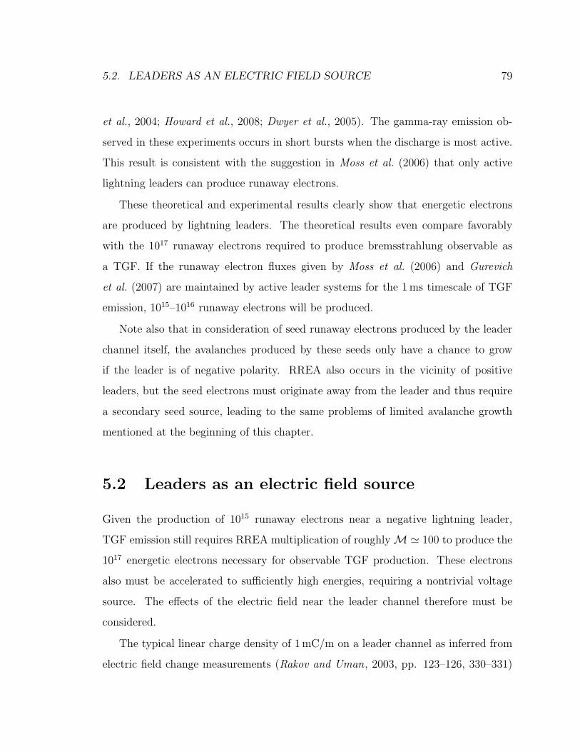
5.2. LEADERS AS AN ELECTRIC FIELD SOURCE 79
et al., 2004; Howard et al., 2008; Dwyer et al., 2005). The gamma-ray emission ob-
served in these experiments occurs in short bursts when the discharge is most active.
This result is consistent with the suggestion in Moss et al. (2006) that only active
lightning leaders can produce runaway electrons.
These theoretical and experimental results clearly show that energetic electrons
are produced by lightning leaders. The theoretical results even compare favorably
with the 1017 runaway electrons required to produce bremsstrahlung observable as
a TGF. If the runaway electron fluxes given by Moss et al. (2006) and Gurevich
et al. (2007) are maintained by active leader systems for the 1 ms timescale of TGF
emission, 1015–1016 runaway electrons will be produced.
Note also that in consideration of seed runaway electrons produced by the leader
channel itself, the avalanches produced by these seeds only have a chance to grow
if the leader is of negative polarity. RREA also occurs in the vicinity of positive
leaders, but the seed electrons must originate away from the leader and thus require
a secondary seed source, leading to the same problems of limited avalanche growth
mentioned at the beginning of this chapter.
5.2 Leaders as an electric field source
Given the production of 1015 runaway electrons near a negative lightning leader,
TGF emission still requires RREA multiplication of roughlyM' 100 to produce the
1017 energetic electrons necessary for observable TGF production. These electrons
also must be accelerated to sufficiently high energies, requiring a nontrivial voltage
source. The effects of the electric field near the leader channel therefore must be
considered.
The typical linear charge density of 1 mC/m on a leader channel as inferred from
electric field change measurements (Rakov and Uman, 2003, pp. 123–126, 330–331)
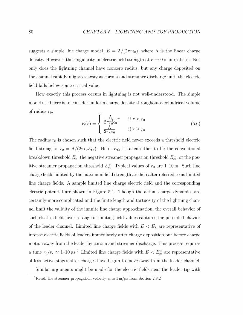
80 CHAPTER 5. LIGHTNING AND TGF PRODUCTION
suggests a simple line charge model, E = Λ/(2πrε0), where Λ is the linear charge
density. However, the singularity in electric field strength at r → 0 is unrealistic. Not
only does the lightning channel have nonzero radius, but any charge deposited on
the channel rapidly migrates away as corona and streamer discharge until the electric
field falls below some critical value.
How exactly this process occurs in lightning is not well-understood. The simple
model used here is to consider uniform charge density throughout a cylindrical volume
of radius r0:
E(r) =
Λ
2πr20ε0
r if r < r0
Λ2πrε0
if r ≥ r0
(5.6)
The radius r0 is chosen such that the electric field never exceeds a threshold electric
field strength: r0 = Λ/(2πε0Eth). Here, Eth is taken either to be the conventional
breakdown threshold Ek, the negative streamer propagation threshold E−cr, or the pos-
itive streamer propagation threshold E+cr. Typical values of r0 are 1–10 m. Such line
charge fields limited by the maximum field strength are hereafter referred to as limited
line charge fields. A sample limited line charge electric field and the corresponding
electric potential are shown in Figure 5.1. Though the actual charge dynamics are
certainly more complicated and the finite length and tortuosity of the lightning chan-
nel limit the validity of the infinite line charge approximation, the overall behavior of
such electric fields over a range of limiting field values captures the possible behavior
of the leader channel. Limited line charge fields with E < Ek are representative of
intense electric fields of leaders immediately after charge deposition but before charge
motion away from the leader by corona and streamer discharge. This process requires
a time r0/vs ' 1–10 µs.2 Limited line charge fields with E < E±cr are representative
of less active stages after charges have begun to move away from the leader channel.
Similar arguments might be made for the electric fields near the leader tip with
2Recall the streamer propagation velocity vs ' 1 m/µs from Section 2.3.2
5.2. LEADERS AS AN ELECTRIC FIELD SOURCE 81
5 10 15 20r (m)
−40
−30
−20
−10
0
10
U(M
V)
0
1
2
3
4
E(M
V/m
)
0 10 20r (m)
Figure 5.1: Line charge radius limits. Electric field and voltage limits for linecharges. The effective radius of the line charge is set such that the electric fieldmagnitude never exceeds Ek ' 3 MV/m
assumption of a point charge at the leader tip, but the magnitude of the effective
point charge on the leader tip is of order the linear charge density times the effective
radius of the wire (Jackson, 2000, 2002)3. A typical charge accumulation near the tip
is therefore Λr0 ' 5 mC. This effective point charge contributes less to the electric
field in the vicinity of the tip of the leader channel than the linear charge density
along the channel near the tip, especially for the regions which contribute most to
RREA multiplication.
The RREA multiplication for such electric fields can be easily calculated:
M = exp
(∫ rb
ra
dr
λ(E(r))
)(5.7)
where the integral in effect calculates the total number of avalanche lengths. The
resulting avalanche multiplication factor for the limited electric field described above
due to various linear charge densities is shown in Figure 5.2.
3The charge density on a charged conducting wire is very close to uniform. Though counterintu-itive, only slight non-uniformity is necessary to remove the electric field imbalance.
82 CHAPTER 5. LIGHTNING AND TGF PRODUCTION
10−1
101
103
105
107
109
M
10−1 100 101 102
Λ (mC/m)
Figure 5.2: RREA growth factor in a limited line charge field. The overallavalanche growth factor over the region where the electric field exceeds ERREA, cal-culated as described in the text. The horizontal dashed line shows M = 100, whilethe horizontal dotted line shows M = 106, the maximum avalanche growth factorallowed by the total thunderstorm potential. The solid, dashed, and dotted curvesrepresent line charges with electric fields limited to E < Ek, E < E−cr, and E < E+
cr,respectively.
Considering a seed source due to leader channels of 1015–1016 as described above,
the required multiplication factor is M ' 10–100 for this population to grow to the
1017 energetic electrons required to produce an observable TGF. Figure 5.2 shows
this growth factor is attained for charge densities Λ & 1–10 mC/m depending on the
limiting electric field strength, easily within the range of values inferred from lightning
observations (Rakov and Uman, 2003, pp. 123–126, 330–331).
5.3 TGF production by lightning current pulses
The above discussion can be put in unified context by consideration of the voltage
and electric field. The typical maximum thunderstorm voltage is ∼ 100 MV, while
any TGF production mechanism must have sufficient voltage to produce 20 MeV
5.3. TGF PRODUCTION BY LIGHTNING CURRENT PULSES 83
electrons. The large populations produced by RREA require an electric field stronger
than ERREA, while the large volumes necessary for RREA cannot support E > Ek.
The effective voltage available and average electric field available to runaway electrons
in the vicinity of limited line charge fields as described above can be estimated from
Equation 5.6 simply by calculating the size and potential difference of the region where
the electric field exceeds ERREA. Static thunderstorm fields are seldom observed above
ERREA but extend up to the maximum potential of the thunderstorm. These voltages
and electric fields are shown in a plot of total potential U vs. average electric field
E in Figure 5.3. The region that satisfies the constraints in potential and electric
field listed above is shaded in grey. Limited line charge electric fields as described
above fall nicely in the allowed range, meeting the required electric field strength and
producing the required voltage.
This mechanism is significantly different from previously proposed TGF produc-
tion mechanisms as it occurs very near the leader channel. The nonuniform and local
electric field that drives the mechanism also differs from the large-scale relatively-
uniform electric fields of the QES and EMP mechanisms discussed in Sections 2.4.1
and 2.4.2. The timescale of the resulting gamma-ray emission is closely tied to the
timescale of leader activity.
Lightning timescales vary from microseconds to seconds as listed in Table 5.1.
Leader activity takes place on a wide range of timescales from HF pulses from leader
stepping (3 mics) to dart leader processes (2 ms). The timescales that best match the
TGF timescale are current pulses indicative of leader activity throughout the lightning
system (return strokes, M-components, and K-changes), suggesting that large bursts
of leader activity are a possible source of TGFs, consistent with the discussion in
Section 5.1 where activity over a 1 ms timescale was required to produce a large seed
population. This connection between current pulse timescale and TGF timescale is
very useful as existing mechanisms do not fully address the TGF timescale. The
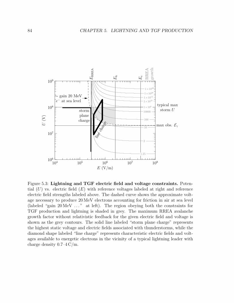
84 CHAPTER 5. LIGHTNING AND TGF PRODUCTION
106
107
108
109
U(V
)
104 105 106 107 108
E (V/m)
1×1030
1×10²⁰
1×10¹⁴
1×10¹⁰
1×10⁶
10000
100
10
2
1.25
stormplanecharge
line
char
ge max obs. Eγ
typical maxstorm U
ER
RE
A
Ek
Ec
RR
EA
grow
th
∼ gain 20 MeVe− at sea level
Figure 5.3: Lightning and TGF electric field and voltage constraints. Poten-tial (U) vs. electric field (E) with reference voltages labeled at right and referenceelectric field strengths labeled above. The dashed curve shows the approximate volt-age necessary to produce 20 MeV electrons accounting for friction in air at sea level(labeled “gain 20 MeV . . . ” at left). The region obeying both the constraints forTGF production and lightning is shaded in grey. The maximum RREA avalanchegrowth factor without relativistic feedback for the given electric field and voltage isshown as the grey contours. The solid line labeled “storm plane charge” representsthe highest static voltage and electric fields associated with thunderstorms, while thediamond shape labeled “line charge” represents characteristic electric fields and volt-ages available to energetic electrons in the vicinity of a typical lightning leader withcharge density 0.7–4 C/m.
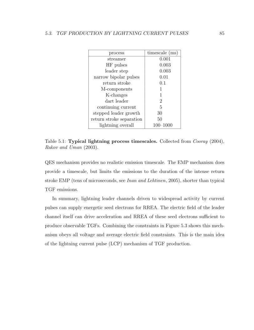
5.3. TGF PRODUCTION BY LIGHTNING CURRENT PULSES 85
process timescale (ms)streamer 0.001
HF pulses 0.003leader step 0.003
narrow bipolar pulses 0.01return stroke 0.1
M-components 1K-changes 1dart leader 2
continuing current 5stepped leader growth 30
return stroke separation 50lightning overall 100–1000
Table 5.1: Typical lightning process timescales. Collected from Cooray (2004),Rakov and Uman (2003).
QES mechanism provides no realistic emission timescale. The EMP mechanism does
provide a timescale, but limits the emissions to the duration of the intense return
stroke EMP (tens of microseconds, see Inan and Lehtinen, 2005), shorter than typical
TGF emissions.
In summary, lightning leader channels driven to widespread activity by current
pulses can supply energetic seed electrons for RREA. The electric field of the leader
channel itself can drive acceleration and RREA of these seed electrons sufficient to
produce observable TGFs. Combining the constraints in Figure 5.3 shows this mech-
anism obeys all voltage and average electric field constraints. This is the main idea
of the lightning current pulse (LCP) mechanism of TGF production.
86 CHAPTER 5. LIGHTNING AND TGF PRODUCTION
5.4 Lightning current pulse mechanism predictions
The LCP mechanism outlined above can be used to make predictions about TGF
coincidence with lightning, production altitude, and initial photon directional distri-
bution. These predictions are testable with satellite and lightning observation.
As the LCP mechanism produces TGFs with lightning leaders, an almost trivial
prediction is that TGFs should never be observed without lightning. It is useful to
make this an explicit prediction as it has been suggested that some TGFs can occur
without lightning. At the time of this writing, however, there are no clear candidate
TGF observations believed to occur without lightning. In particular, though there
have been cases suggested where TGFs were observed in locations where lightning
could not have occurred (i.e., over the Sahara desert, Smith et al., 2007) or should
have been observed had it occurred (Cohen et al., 2007), these cases have since been
explained either as indirect observations of electrons trapped on the geomagnetic
field produced by distant TGFs (see for example the beautiful modeling results in
Dwyer et al. (2008a) and other candidate observations in Carlson et al. (2009a)) or
as experimental anomalies4. This prediction can be tested by TGF observations near
lightning detector networks sensitive enough to detect even weak intra-cloud lightning
activity. If a TGF is observed under circumstances convincingly devoid of lightning,
other mechanisms must be considered.
Less trivially, the LCP mechanism requires active lightning leaders in order to
ensure RREA seed production. Lightning leader activity is driven by currents flow-
ing on the channel, so direct TGF production by leaders predicts that TGF emission
must always be accompanied not only by lightning as a whole but by leader activity
as evidenced by current flow in the leader channel network. As such currents emit
4Despite appearances, the case mentioned in Cohen et al. (2007), though presented as a TGFclearly not associated with lightning, was later retracted as an instrumental effect. The moral: whenyou have hundreds of events, one-in-a-hundred is actually quite frequent.
5.4. LIGHTNING CURRENT PULSE MECHANISM PREDICTIONS 87
electromagnetic waves, the mechanism as described predicts a close time coincidence
between TGF emission and radio emission. This is overall consistent with observa-
tions, though as mentioned in Section 1.2.4, timing uncertainty limits the accuracy of
existing analyses. This prediction may also be tested with accurate timing in the sen-
sitive coincident lightning observations necessary to detect weak intra-cloud lightning
activity mentioned above.
The LCP mechanism predicts TGF production very nearby lightning activity. In
particular, TGFs should be produced at effectively the same altitude as lightning
discharge. Typical lightning spans a range in altitudes, often up to the upper regions
of the thunderstorm but does not commonly extend above cloud-tops. The altitude
of high-altitude lightning is therefore less than that of the tropopause.5 Tropopause
height depends on the intensity of solar heating and thus on the latitude and season,
but typically varies from 11–18 km over the latitude range covered by RHESSI and
BATSE (Blair and Fite, 1957, p. 118). The altitude range predicted for TGF pro-
duction by lightning in the upper regions of a thunderstorm is therefore consistent
with the spectral constraints derived in Section 3.2.1 in regions of high tropopause
height. High tropopause height is confined to the tropics where both the majority of
lightning occurs and the majority of TGFs are observed, a fact suggested to explain
the relative lack of TGFs over regions where lightning is otherwise common such
as the continental United States and southeastern Australia (Williams et al., 2006).
The validity of the LCP mechanism can therefore be tested by searching for TGFs
with spectra requiring production significantly above the tropopause, as such TGFs
cannot be produced directly by lightning leaders.
As the lightning parameters used in this analysis are not extreme, it is expected
5The tropopause marks the boundary between the troposphere and the stratosphere. The tro-posphere, the “turning” or turbulent and well-mixed portion of the atmosphere is driven primarilyby solar heating from below and the instabilities that result. The stratosphere, the “layered” atmo-sphere, is not as well-mixed and is driven primarily by heating from above due to ozone absorptionof ultraviolet light from the sun. What we know as weather occurs entirely in the troposphere.
88 CHAPTER 5. LIGHTNING AND TGF PRODUCTION
that gamma-ray emission often accompanies lightning leaders. This is consistent with
observations (Dwyer et al., 2003; Dwyer et al., 2004; Howard et al., 2008; Dwyer et al.,
2005). However, not all lightning produces TGFs. First note that not all lightning-
induced gamma-ray emission is observable by satellites. Low-altitude emissions are
heavily attenuated and emissions of relatively few photons are difficult to distinguish
from noise. The mechanism we discuss here may require uncommonly large current
pulses to drive sufficient activity throughout a high-altitude leader network to produce
an observable TGF. Higher altitudes are also favorable due to lower atmospheric
density, lower frictional losses, and correspondingly greater RREA growth rates. Also
note that as the global frequency of TGFs is not known, a high rate of low-intensity
gamma-ray emission events as suggested by the mechanism described above may
indeed be present.
The electric fields that drive TGF production in the LCP mechanism are nonuni-
form and diverge away from the leader channel. The photons produced by energetic
electrons driven by such electric fields also diverge away from the leader channel in
a very broad beam. This broad beam is nominally consistent with the beaming con-
straints discussed in Sections 3.2.1 and 3.2.3. Results from Hazelton et al. (2009) also
indicate TGF data are better fit by beams broader than those due to bremsstrahlung
and RREA alone, so the broad beams naturally produced by the LCP mechanism
should be considered. More detailed spectral analysis and careful TGF-lightning co-
incidence studies can be used to test this prediction, as such analyses may indicate
narrower beams than can be produced by leader electric fields.
These predictions can all be tested with satellite and radio data. In particular,
data from the Fermi Gamma-ray Burst Monitor (GBM), the AGILE satellite,6 the
6Astro-rivelatore Gamma a Immagini LEggero, an Italian Space Agency satellite.
5.4. LIGHTNING CURRENT PULSE MECHANISM PREDICTIONS 89
ASIM experiment,7 and the TARANIS satellite8 could be used to provide the high
precision, high energy-resolution spectra necessary to accurately measure the pro-
duction altitude to confirm or refute close association with lightning. The ADELE
experiment9 will provide clear results on the likelihood of frequent low-intensity TGF-
like emissions predicted by the relatively common parameters suggested for lightning-
driven TGF production. Cameras on ASIM and TARANIS, together with more mod-
ern radio data, will help accurately measure the properties of coincident lightning and
the nature of the temporal and spatial association between lightning and TGF pro-
duction. This knowledge will help determine the validity of the LCP mechanism of
TGF production mechanism described above.
7The Atmosphere-Space Interactions Monitor, a European Space Agency experiment for theinternational space station.
8Named for the Celtic god of thunder and as the Tool for the Analysis of RAdiation from lightNIngand Sprites, a French (CNES) satellite.
9The Airborne Detector for Energetic Lightning Emissions, an aircraft-borne gamma-ray detectorexperiment funded by the NSF.
90 CHAPTER 5. LIGHTNING AND TGF PRODUCTION
5.5 Comparison to relativistic feedback TGF pro-
duction
An alternative mechanism to LCP TGF production is the relativistic feedback mecha-
nism in static thunderstorm electric fields as suggested by Dwyer (2009). Relativistic
feedback as described in Section 2.2.1 also removes the restriction on the seed pop-
ulation by effectively allowing an initial avalanche to seed a second generation of
avalanches. This requires the production of new effective seed particles by photon
and positron propagation back to near the starting point of the original avalanche. As
such, relativistic feedback depends on the size and shape of the electric field region.
Dwyer (2003) gives constraints on the size and shape for uniform electric fields. For
instance, a 1 MV/m electric field requires a size of at least 100 m (available poten-
tial U ≥ 100 MV) for relativistic feedback to occur. These are shown in Figure 5.4
superimposed on the central region of Figure 5.3.
Relativistic feedback in thunderstorm conditions therefore requires relatively high
electric field over a relatively long length-scale. Dwyer (2009) suggests these condi-
tions may be met in a thunderstorm and that TGFs may result.
Relativistic feedback in thunderstorm electric fields as a TGF source has several
key characteristics that distinguish it from LCP TGF production. Relativistic feed-
back does not require a lightning discharge, and therefore is a possible explanation if
TGFs are produced without lightning. Thunderstorm static electric fields are typi-
cally quite uniform, so relativistic feedback predicts photon emissions with relatively
narrow directional distribution. Finally, once initiated, relativistic feedback continues
to grow until the electric field either naturally decays or is forced to decay by the cur-
rents produced in RREA. The characteristic timescale of the decay of the electric field
under relativistic feedback process is 20 µs, shorter than the typical TGF timescale,
but is very strongly dependent on the electric field for E near ERREA and can be
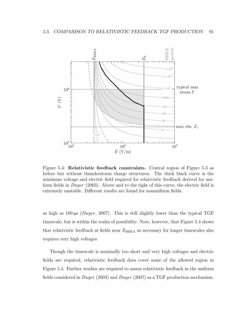
5.5. COMPARISON TO RELATIVISTIC FEEDBACK TGF PRODUCTION 91
107
108
U(V
)
105 106 107
E (V/m)
1×10¹⁴
1×10¹⁰
1×10⁶
10000
500
100
30
10
521.25
max obs. Eγ
typical maxstorm U
ER
RE
A
Ek
RR
EA
grow
thFigure 5.4: Relativistic feedback constraints. Central region of Figure 5.3 asbefore but without thunderstorm charge structures. The thick black curve is theminimum voltage and electric field required for relativistic feedback derived for uni-form fields in Dwyer (2003). Above and to the right of this curve, the electric field isextremely unstable. Different results are found for nonuniform fields.
as high as 100 µs (Dwyer , 2007). This is still slightly lower than the typical TGF
timescale, but is within the realm of possibility. Note, however, that Figure 5.4 shows
that relativistic feedback at fields near ERREA as necessary for longer timescales also
requires very high voltages.
Though the timescale is nominally too short and very high voltages and electric
fields are required, relativistic feedback does cover some of the allowed region in
Figure 5.4. Further studies are required to assess relativistic feedback in the uniform
fields considered in Dwyer (2003) and Dwyer (2007) as a TGF production mechanism.
92 CHAPTER 5. LIGHTNING AND TGF PRODUCTION
5.5.1 Relativistic feedback in nonuniform fields
As relativistic feedback may be relevant to thunderstorm electric fields, it may also
be relevant to the nonuniform electric fields surrounding lightning leader channels. In
such conditions the confinement of the electric field renders it much less likely that
a photon or positron will make its way to regions favorable to the production of a
second generation of avalanches. This depends on the geometry and polarity of the
electric field, however, so it is useful to measure the feedback behavior of such fields.
Here GEANT4 simulations of RREA are used as the basis for a feedback measure-
ment scheme. The limited electric field described above is used to drive RREA of a
population of seed 1 MeV electrons placed in the high potential energy region of the
field with their velocities pointing in the direction of avalanche growth. As RREA of
this population proceeds, the total number of electrons produced is recorded. Sec-
ondary particles produced by electrons are tracked without limitation, including brem-
sstrahlung photons and positrons resulting from pair production. However, electrons
produced by photons or positrons are classified as second-generation seed particles and
are recorded and removed from the simulation. The result of such simulations is the
number of electrons produced in the first generation avalanche and the positions and
momenta of seed particles for the next generation. The potential avalanche growth
of these possible second-generation seed particles is then calculated with Equation
5.7 integrated along the path of the avalanche that would result. The sum of these
avalanche multiplication factors for all of the possible second-generation seed elec-
trons is an estimate of the possible size of the second generation. The quotient of
this estimate of the second generation population with the measured first generation
population size is a measure of the feedback factor Γ. If Γ < 1, the second generation
is smaller than the first and the overall activity of the system should decay away with
time, while if Γ > 1 the second generation is bigger than the first generation, and
relativistic feedback effects must be considered.
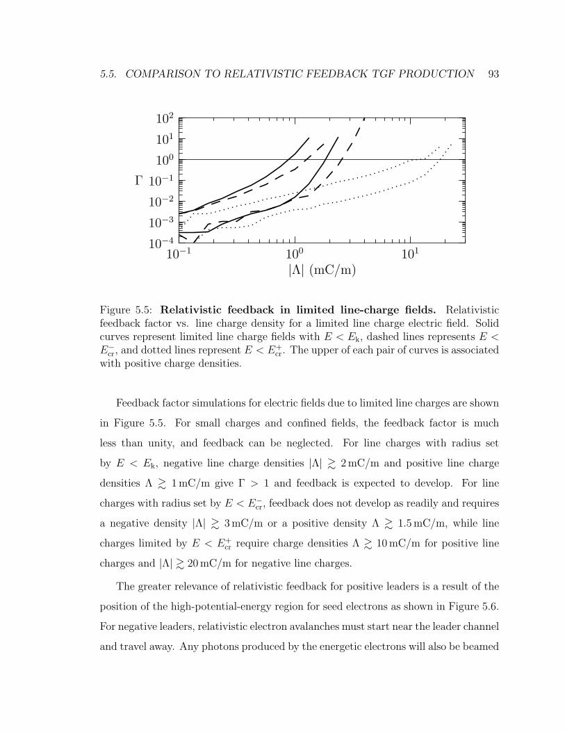
5.5. COMPARISON TO RELATIVISTIC FEEDBACK TGF PRODUCTION 93
10−4
10−3
10−2
10−1
100
101
102
Γ
10−1 100 101
|Λ| (mC/m)
Figure 5.5: Relativistic feedback in limited line-charge fields. Relativisticfeedback factor vs. line charge density for a limited line charge electric field. Solidcurves represent limited line charge fields with E < Ek, dashed lines represents E <E−cr, and dotted lines represent E < E+
cr. The upper of each pair of curves is associatedwith positive charge densities.
Feedback factor simulations for electric fields due to limited line charges are shown
in Figure 5.5. For small charges and confined fields, the feedback factor is much
less than unity, and feedback can be neglected. For line charges with radius set
by E < Ek, negative line charge densities |Λ| & 2 mC/m and positive line charge
densities Λ & 1 mC/m give Γ > 1 and feedback is expected to develop. For line
charges with radius set by E < E−cr, feedback does not develop as readily and requires
a negative density |Λ| & 3 mC/m or a positive density Λ & 1.5 mC/m, while line
charges limited by E < E+cr require charge densities Λ & 10 mC/m for positive line
charges and |Λ| & 20 mC/m for negative line charges.
The greater relevance of relativistic feedback for positive leaders is a result of the
position of the high-potential-energy region for seed electrons as shown in Figure 5.6.
For negative leaders, relativistic electron avalanches must start near the leader channel
and travel away. Any photons produced by the energetic electrons will also be beamed
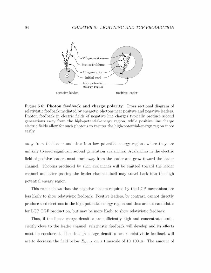
94 CHAPTER 5. LIGHTNING AND TGF PRODUCTION
Figure 5.6: Photon feedback and charge polarity. Cross sectional diagram ofrelativistic feedback mediated by energetic photons near positive and negative leaders.Photon feedback in electric fields of negative line charges typically produce secondgenerations away from the high-potential-energy region, while positive line chargeelectric fields allow for such photons to reenter the high-potential-energy region moreeasily.
away from the leader and thus into low potential energy regions where they are
unlikely to seed significant second generation avalanches. Avalanches in the electric
field of positive leaders must start away from the leader and grow toward the leader
channel. Photons produced by such avalanches will be emitted toward the leader
channel and after passing the leader channel itself may travel back into the high
potential energy region.
This result shows that the negative leaders required by the LCP mechanism are
less likely to show relativistic feedback. Positive leaders, by contrast, cannot directly
produce seed electrons in the high potential energy region and thus are not candidates
for LCP TGF production, but may be more likely to show relativistic feedback.
Thus, if the linear charge densities are sufficiently high and concentrated suffi-
ciently close to the leader channel, relativistic feedback will develop and its effects
must be considered. If such high charge densities occur, relativistic feedback will
act to decrease the field below ERREA on a timescale of 10–100 µs. The amount of
5.6. SUMMARY 95
energy released as energetic bremsstrahlung in this process is unknown and requires
detailed study with a full self-consistent mechanism of RREA, relativistic feedback,
the relativistic currents, and conductivity enhancements that result.
5.6 Summary
The maximum RREA growth factor together with the maximum allowed energetic
seed particle population are not sufficient to account for observable TGFs. This
realization leads to the suggestion of negative lightning leader channels as the key
driving force behind TGF production, providing both RREA seed source and driving
electric field. Evidence for the seed source is seen in experiments and total seed flux
derived in the literature for active leader channels is consistent with TGF production
if the leaders are driven to activity by current pulses for the ∼ 1 ms TGF timescale.
Estimates of the electric field near negative leader channels give sufficient avalanche
multiplication of the seed flux if the linear charge density |Λ| > 1–10 mC/m (de-
pending on the effective radius of the line charge), within range of values observed
in experiments. The total voltage and electric field constraints shown in Figure 5.3
are satisfied by this mechanism, leading to the suggestion of lightning current pulse
(LCP) TGF production. Relativistic feedback may also be relevant, especially for
positive leader channels, though further analysis is required. TGFs may therefore be
produced by active leader channels driven by current pulses. The core idea of LCP
TGF production is available in the literature in Carlson et al. (2009b).
Chapter 6
Lightning TGF production model
The analyses in Chapter 5 suggest that the electric fields of negative lightning leaders,
together with RREA seed production by active leaders driven by lightning current
pulses can drive TGF production, dubbed the lightning current pulse (LCP) TGF pro-
duction mechanism. The results of Chapter 5 indicate that the LCP TGF production
mechanism satisfies the electric field and voltage constraints. The LCP mechanism
may produce the overall energy required if sufficient leader activity occurs in the
timescale of TGF emission as suggested by the timescale of large current pulses in
leader channels.
The key question is whether or not the current pulses in leader systems actually
are capable of driving TGF production, and if so what currents are required. This
chapter describes a model of the LCP TGF production mechanism. Lightning cur-
rent pulse propagation is modeled by the method of moments. This model is used
to determine temporal and spatial dependence of the electric field over volumes near
the leader. This electric field is then used to drive GEANT4 simulations of RREA.
The properties of the resulting RREA including the energy spectra and photon direc-
tional distributions are derived and compared to the constraints on TGF production
discussed in Chapters 3 and 5.
96
6.1. LIGHTNING ELECTRIC FIELD MODEL 97
6.1 Lightning electric field model
The electric field surrounding a lightning leader is a combination of the ambient
thunderstorm electric field (Es) and the electric field due to charges on and currents
flowing along the leader channel (El). The total electric field Et = Es +El determines
the flow of charges on the resistive leader channel. The time evolution of the system
of charges and currents is also affected by the development of the channel. Sudden
extensions and connections of the channel with regions of positive or negative charge
lead to current pulses. Such pulses are proposed as associated with the leader activity
driving RREA seed production and TGF emission in the LCP mechanism discussed
in Chapter 5. A full model of the behavior of the currents and charges on the lightning
channel is therefore useful for consideration of TGF production by such currents.
Such models can be constructed in several ways, depending on the phenomenon
of interest. Complete reviews can be found in Rakov and Uman (1998) and Baba
and Rakov (2007). Existing modeling efforts treat a range of processes, from the
plasma physics of the leader channel to electromagnetic processes involved in current
flow. Plasma physics models strive to treat the leader by solving the gas dynamics
equations involving conservation of energy, momentum, and mass, together with the
equation of state of the plasma and energy input from applied currents. Electro-
magnetic models treat the leader as an abstract resistive or conducting channel and
solve Maxwell’s equations together with Ohm’s law, allowing determination of the
currents and electromagnetic fields. Higher level models are also possible, involv-
ing further approximations such as treatment of the channel as a transmission line
(solving the telegrapher’s equations) and “engineering models” that merely assume
properties grossly consistent with observed lightning discharges.
Here, the electric field produced by the lightning channel as a driver of energetic
98 CHAPTER 6. LIGHTNING TGF PRODUCTION MODEL
electron physics requires an electromagnetic model of the lightning channel. Electro-
magnetic models solve Maxwell’s equations by a variety of techniques. One approach
is by finite-difference methods (for instance, Noda and Yokoyama, 2002), which con-
vert Maxwell’s equations to a set of matrix equations describing the evolution of the
charges, currents, and electromagnetic fields on a grid spanning the volume of interest.
As lightning leaders have very tortuous structure, accurate representation of the fields
near the channel requires a very fine grid with correspondingly large memory require-
ments for full 3-dimensional simulation domains. The approach used here instead uses
the method of moments, which converts Maxwell’s equations in retarded-time inte-
gral form into a system of matrix equations involving segments of the channel (Rao,
1999, Chapter 2). This conversion reduces the memory requirements and allows for
treatment of detailed 3-dimensional channel structures.
The starting point for the electromagnetic model constructed herein is the electric
field integral equation which gives the electric field at any point in terms of the charges
and currents present in the system (EFIE, eq. 6.55 Jackson, 1999, pp. 247):
Et(x, t) =1
4πε0
∫d3x′
R
R2[ρ(x′, t′)]ret +
R
cR
[∂ρ(x′, t′)∂t′
]ret
− 1
c2R
[∂J(x′, t′)
∂t′
]ret
(6.1)
Where ρ is the volume charge density, J is the current density, R = x− x′, R = |R|,R = R/R, and the subscript “ret” indicates that the term in brackets is to be
evaluated at the retarded time t′ = t − R/c. The EFIE can be most readily derived
from the retarded-time integral solutions for the electric scalar potentials Φ and the
magnetic vector potential A, but the details are not illustrative (see Jackson, 1999,
pp. 246–7).
The electric field and the current are related by Ohm’s law:
J = σEt (6.2)
6.1. LIGHTNING ELECTRIC FIELD MODEL 99
Note that this simple form of Ohm’s law ignores the effects of magnetic fields. This
assumption is justified by the relatively low velocity of the electrons that carry the
bulk of the charge in a lightning stroke together with the high collision frequency for
such electrons at altitudes characteristic of lightning.
Together with the equation of charge conservation,
∂ρ
∂t+∇ · J = 0 (6.3)
Equations 6.1 and 6.2 provide a full system of integro-differential and partial differ-
ential equations describing the time evolution of charges and currents in a resistive
or conducting system.
6.1.1 Method of moments simulation
It remains to solve the system of Equations 6.1, 6.2 and 6.3 in the context of lightning.
Due to the difficulty of solving integral equations, let alone integro-partial-differential
equations, approximations and simplifications must be made. Here the thin wire
approximation and the method of moments are used. The approach used here is
similar to and motivated by the approach in Miller et al. (1973).
The thin wire approximation treats Equation 6.1 as a line integral over the leader
channel instead of a volume integral. This simplification is accomplished by assuming
that the currents flow purely in the direction of the leader and that the charges
and currents reside at the center of the leader while the electric field is evaluated
at the surface of the channel. This assumption allows the replacement of R with
L =√R2 + a2, effectively preventing any quantity from being evaluated at points
closer than a distance a away from the center of the channel. This approximation
is justified if the channel is sufficiently longer than its radius, typically by at least a
factor of 4. This condition is clearly applicable to lightning channels linear on a scale
100 CHAPTER 6. LIGHTNING TGF PRODUCTION MODEL
of 100 m with radius a ' 1–10 m.
Application of the thin wire approximation allows integration over the transverse
dimensions of the wire, giving:
El(x, t) =1
4πε0
∫ds′
R
L2[Λ(s′, t′)]ret +
R
cL
[∂Λ(s′, t′)
∂t′
]ret
− s
c2L
[∂I(s′, t′)∂t′
]ret
(6.4)
where s′ is a linear position coordinate along the leader, s is a unit vector in the
direction parallel to the channel, Λ is the linear charge density, and I is the current
in the channel. Charge conservation and Ohm’s law similarly become
∂Λ
∂t+∂I
∂s= 0 (6.5)
IRl = Et · s (6.6)
where Rl is the resistance per unit length of the channel, Et = Es +El, El is evaluated
as in Equation 6.4 and Es is the applied electric field due to thunderstorm charges not
on the leader channel. Ohm’s law (Equation 6.6) can then be applied to the electric
field integral equation to close the system and give an equation for I(s, t) in terms of
an integral of Λ and I. The quantity Λ can in turn be calculated as an integral of I,
Λ(s, t) = −∫ t
−∞
∂
∂sI(s, ξ)dξ (6.7)
leaving an equation for I in terms of past and present values of I, integrals of I, and
derivatives of I.
The method of moments then exploits the linearity of the integro-differential oper-
ator in Equation 6.4 to convert it into an algebraic equation. The method of moments
proceeds by breaking the charges and currents into segments. The discretization
scheme used here is shown schematically in Figure 6.1. The charge distribution is
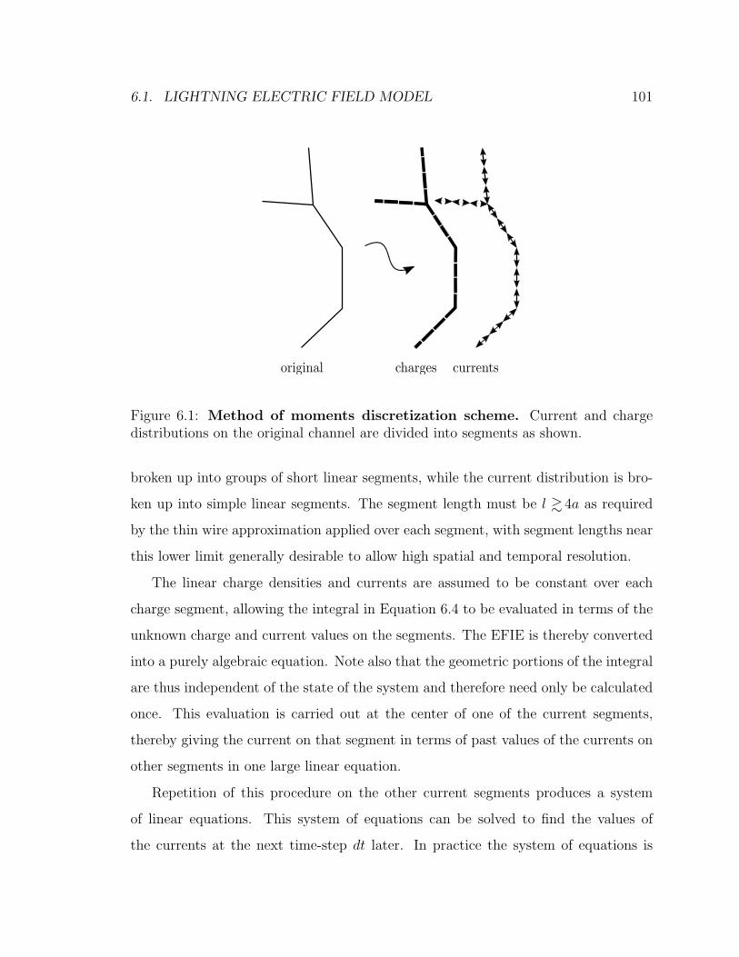
6.1. LIGHTNING ELECTRIC FIELD MODEL 101
Figure 6.1: Method of moments discretization scheme. Current and chargedistributions on the original channel are divided into segments as shown.
broken up into groups of short linear segments, while the current distribution is bro-
ken up into simple linear segments. The segment length must be l & 4a as required
by the thin wire approximation applied over each segment, with segment lengths near
this lower limit generally desirable to allow high spatial and temporal resolution.
The linear charge densities and currents are assumed to be constant over each
charge segment, allowing the integral in Equation 6.4 to be evaluated in terms of the
unknown charge and current values on the segments. The EFIE is thereby converted
into a purely algebraic equation. Note also that the geometric portions of the integral
are thus independent of the state of the system and therefore need only be calculated
once. This evaluation is carried out at the center of one of the current segments,
thereby giving the current on that segment in terms of past values of the currents on
other segments in one large linear equation.
Repetition of this procedure on the other current segments produces a system
of linear equations. This system of equations can be solved to find the values of
the currents at the next time-step dt later. In practice the system of equations is
102 CHAPTER 6. LIGHTNING TGF PRODUCTION MODEL
nearly diagonal as most of the contributions to the electric field are due to the known
past history of the system. Linear interpolation in time is used to evaluate these past
charge and current values. However, if the geometry of the system is such that certain
charges and currents fall less than a distance of c dt apart, the value of one current at
the next time-step depends on the unknown value of another current at the same time-
step. The evaluation of the contribution of one current to the other therefore requires
interpolation involving unknown values and produces off-diagonal components in the
system of equations. In particular, as the current and charge segments are offset, the
adjacent charge values are often separated from the currents that feed them by less
than c dt. The necessary interpolation improves the stability of the system effectively
by providing immediate feedback about the effect of the current in question on the
charges it connects, but requires solution of an approximately tridiagonal system of
linear equations.
The solution of the system of equations gives the next set of currents in the
system. Note that the matrix that describes the equations of this scheme depends
only on the geometry of the system and thus is not time dependent. Any matrix
inversions involved in the solution to the system necessary at each time-step can thus
be calculated only once at the start of the simulation and reused thereafter, though
in practice it can be faster to repeatedly invert the sparse matrices involved than
to repeatedly multiply dense matrices. Simple integration of currents in and out of
the charge segments then gives the corresponding set of charge values. Repeating
the process gives the time evolution of the current and charge values in the system.
Each step in the simulation therefore involves an integral over past values of the
charges and currents to calculate the electric field, construction of a matrix equation
incorporating the channel resistance and any dependence of the electric field on the
unknown currents, solution of the resulting linear system to determine the unknown
currents, and integration of the currents to determine the unknown charges.
6.1. LIGHTNING ELECTRIC FIELD MODEL 103
The system is implemented computationally as approximately 700 lines of Haskell,
a purely functional programming language featuring garbage collection and an opti-
mizing native-code compiler. The Haskell functions make use of the HMatrix1 bind-
ings to the GNU Scientific Library,2 BLAS,3, LAPACK4, and custom bindings to
CXSparse for sparse matrix operations.5 Geometric and interpolation factors are
pre-calculated and used repeatedly.
Though written in a high-level language, the results are sufficiently fast that fur-
ther optimization has not been necessary for systems with fewer than a few thousand
current segments. As the bulk of the computation time is spent calculating sums
over past current and charge states in the electric field integral, large performance
gains could be obtained by splitting the workload among many processors on a multi-
processor machine. Further performance gains could be obtained by vectorizing the
code for execution on a graphics processor. Graphical output is provided by simple
OpenGL code. Electric field output is supported on Cartesian grids covering regions
of interest. The scheme described is stable if the conditions of the thin wire approx-
imation are met. High frequency noise sometimes appears but can be removed with
a simple averaging procedure as discussed in Smith (1990).
The code has been validated by comparison to results given in Poggio et al. (1973)
for a thin wire antenna excited by an electric field pulse at its center. The current
induced at the center of the antenna is shown in Figure 6.2. The results are in
good agreement with the possible exception of the high-frequency components which
dissipate slightly more quickly in the current pulse simulation than in the results from
Poggio et al. (1973).
The simulation has also been validated in the context of lightning return strokes
1http://hackage.haskell.org/package/hmatrix2http://www.gnu.org/software/gsl/3http://www.netlib.org/blas/4http://www.netlib.org/lapack/5http://www.cise.ufl.edu/research/sparse/CXSparse/
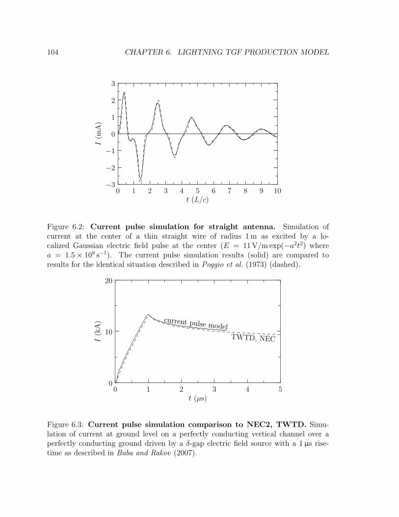
104 CHAPTER 6. LIGHTNING TGF PRODUCTION MODEL
−3
−2
−1
0
1
2
3
I(m
A)
0 1 2 3 4 5 6 7 8 9 10t (L/c)
Figure 6.2: Current pulse simulation for straight antenna. Simulation ofcurrent at the center of a thin straight wire of radius 1 m as excited by a lo-calized Gaussian electric field pulse at the center (E = 11 V/m exp(−a2t2) wherea = 1.5× 10⁹ s−1). The current pulse simulation results (solid) are compared toresults for the identical situation described in Poggio et al. (1973) (dashed).
Figure 6.3: Current pulse simulation comparison to NEC2, TWTD. Simu-lation of current at ground level on a perfectly conducting vertical channel over aperfectly conducting ground driven by a δ-gap electric field source with a 1 µs rise-time as described in Baba and Rakov (2007).
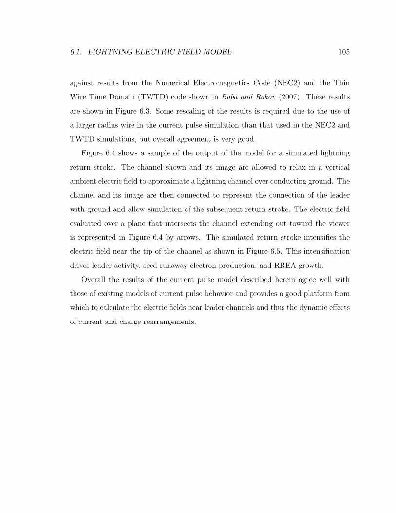
6.1. LIGHTNING ELECTRIC FIELD MODEL 105
against results from the Numerical Electromagnetics Code (NEC2) and the Thin
Wire Time Domain (TWTD) code shown in Baba and Rakov (2007). These results
are shown in Figure 6.3. Some rescaling of the results is required due to the use of
a larger radius wire in the current pulse simulation than that used in the NEC2 and
TWTD simulations, but overall agreement is very good.
Figure 6.4 shows a sample of the output of the model for a simulated lightning
return stroke. The channel shown and its image are allowed to relax in a vertical
ambient electric field to approximate a lightning channel over conducting ground. The
channel and its image are then connected to represent the connection of the leader
with ground and allow simulation of the subsequent return stroke. The electric field
evaluated over a plane that intersects the channel extending out toward the viewer
is represented in Figure 6.4 by arrows. The simulated return stroke intensifies the
electric field near the tip of the channel as shown in Figure 6.5. This intensification
drives leader activity, seed runaway electron production, and RREA growth.
Overall the results of the current pulse model described herein agree well with
those of existing models of current pulse behavior and provides a good platform from
which to calculate the electric fields near leader channels and thus the dynamic effects
of current and charge rearrangements.
106 CHAPTER 6. LIGHTNING TGF PRODUCTION MODEL
Figure 6.4: Realistic lightning channel simulation. Left: a possible lightningchannel. From ground to top the channel is ∼ 1 km tall. Right: the upper portions ofthe channel. The segment that extends toward the viewer is cut by a plane where theelectric field Et is represented by the arrows. In the simulations, the current pulsedue to connection of the channel with its image drives RREA near the tip of thechannel as indicated. Graphics generated by OpenGL.
6.2 RREA in realistic lightning electric fields
The electric fields calculated in the results of the current pulse model described above
can drive RREA. If the current pulse is sufficiently intense as is the case in Figure 6.5,
the electric field increases far above the threshold for runaway relativistic electron
avalanche (ERREA) and can accelerate runaway electrons to high energies and drive
RREA growth. In this section, the fields thus calculated are used to drive GEANT4
simulations of RREA such that the properties of the resulting energetic particles can
be simulated.
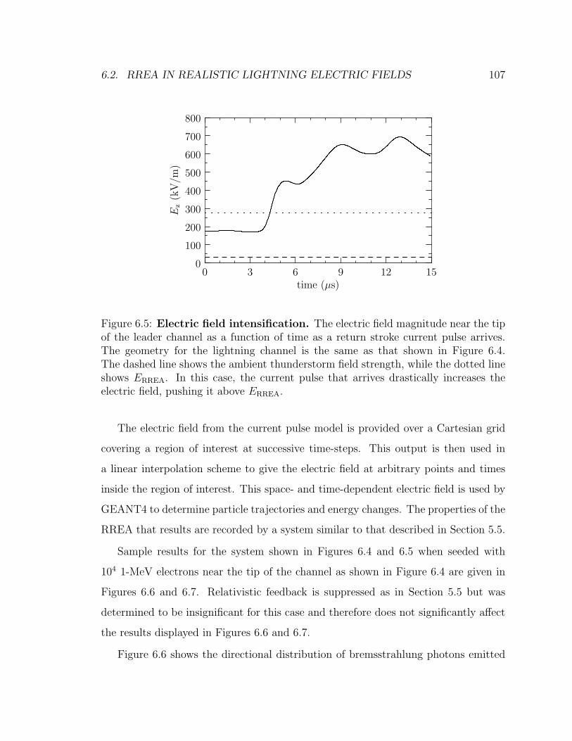
6.2. RREA IN REALISTIC LIGHTNING ELECTRIC FIELDS 107
Figure 6.5: Electric field intensification. The electric field magnitude near the tipof the leader channel as a function of time as a return stroke current pulse arrives.The geometry for the lightning channel is the same as that shown in Figure 6.4.The dashed line shows the ambient thunderstorm field strength, while the dotted lineshows ERREA. In this case, the current pulse that arrives drastically increases theelectric field, pushing it above ERREA.
The electric field from the current pulse model is provided over a Cartesian grid
covering a region of interest at successive time-steps. This output is then used in
a linear interpolation scheme to give the electric field at arbitrary points and times
inside the region of interest. This space- and time-dependent electric field is used by
GEANT4 to determine particle trajectories and energy changes. The properties of the
RREA that results are recorded by a system similar to that described in Section 5.5.
Sample results for the system shown in Figures 6.4 and 6.5 when seeded with
104 1-MeV electrons near the tip of the channel as shown in Figure 6.4 are given in
Figures 6.6 and 6.7. Relativistic feedback is suppressed as in Section 5.5 but was
determined to be insignificant for this case and therefore does not significantly affect
the results displayed in Figures 6.6 and 6.7.
Figure 6.6 shows the directional distribution of bremsstrahlung photons emitted
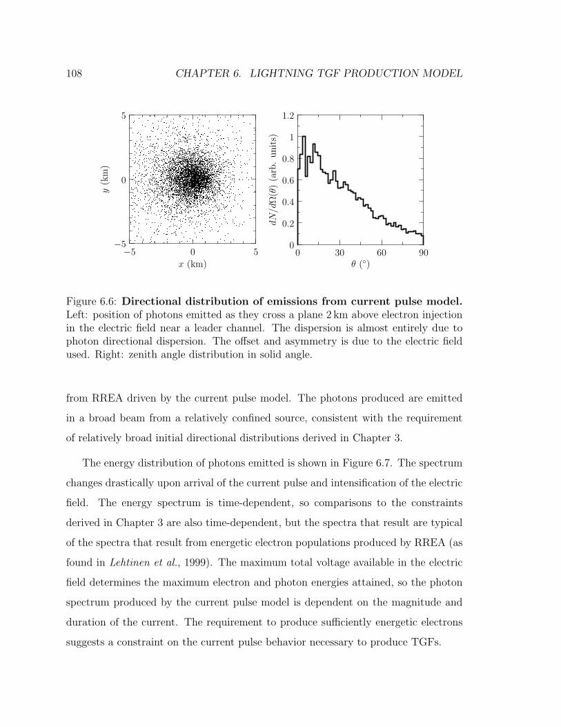
108 CHAPTER 6. LIGHTNING TGF PRODUCTION MODEL
−5
0
5y
(km
)
−5 0 5
x (km)
0
0.2
0.4
0.6
0.8
1
1.2
dN
/dΩ
(θ)
(arb
.unit
s)
0 30 60 90θ ()
Figure 6.6: Directional distribution of emissions from current pulse model.Left: position of photons emitted as they cross a plane 2 km above electron injectionin the electric field near a leader channel. The dispersion is almost entirely due tophoton directional dispersion. The offset and asymmetry is due to the electric fieldused. Right: zenith angle distribution in solid angle.
from RREA driven by the current pulse model. The photons produced are emitted
in a broad beam from a relatively confined source, consistent with the requirement
of relatively broad initial directional distributions derived in Chapter 3.
The energy distribution of photons emitted is shown in Figure 6.7. The spectrum
changes drastically upon arrival of the current pulse and intensification of the electric
field. The energy spectrum is time-dependent, so comparisons to the constraints
derived in Chapter 3 are also time-dependent, but the spectra that result are typical
of the spectra that result from energetic electron populations produced by RREA (as
found in Lehtinen et al., 1999). The maximum total voltage available in the electric
field determines the maximum electron and photon energies attained, so the photon
spectrum produced by the current pulse model is dependent on the magnitude and
duration of the current. The requirement to produce sufficiently energetic electrons
suggests a constraint on the current pulse behavior necessary to produce TGFs.
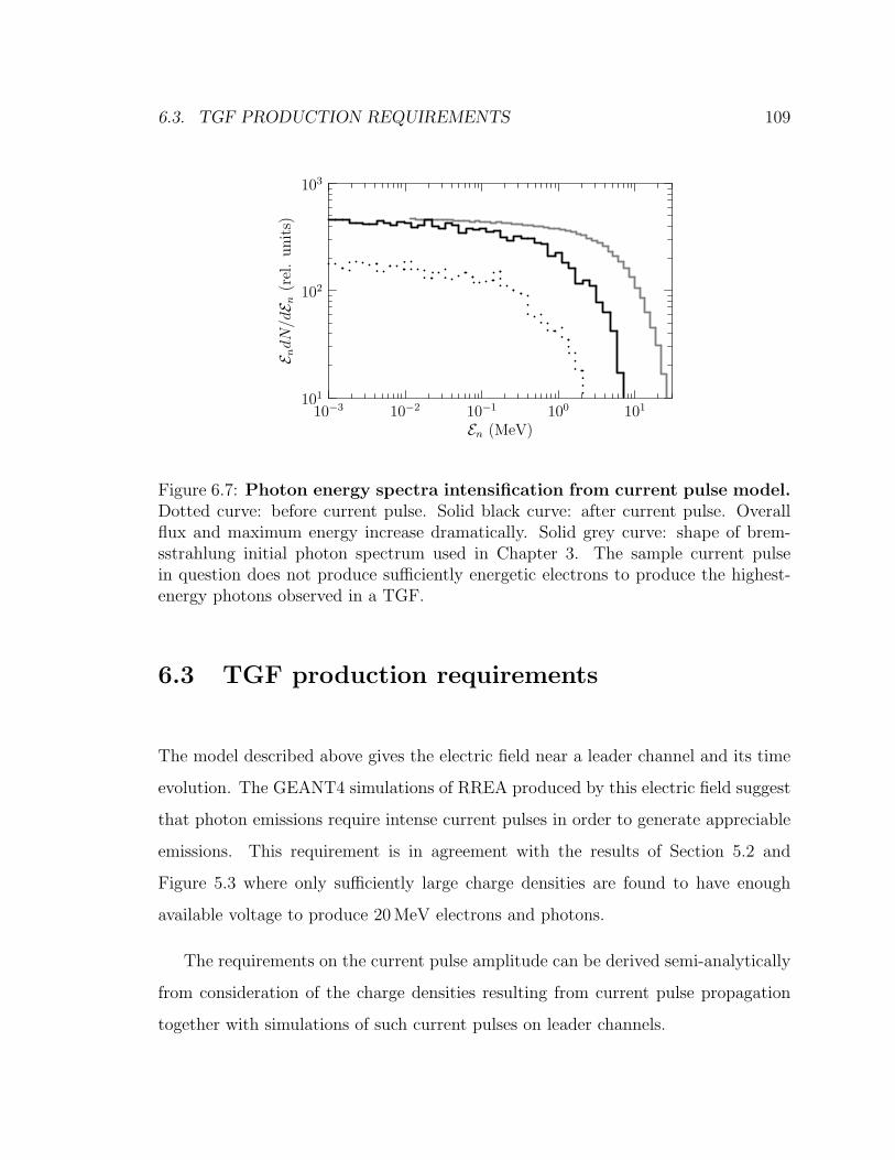
6.3. TGF PRODUCTION REQUIREMENTS 109
Figure 6.7: Photon energy spectra intensification from current pulse model.Dotted curve: before current pulse. Solid black curve: after current pulse. Overallflux and maximum energy increase dramatically. Solid grey curve: shape of brem-sstrahlung initial photon spectrum used in Chapter 3. The sample current pulsein question does not produce sufficiently energetic electrons to produce the highest-energy photons observed in a TGF.
6.3 TGF production requirements
The model described above gives the electric field near a leader channel and its time
evolution. The GEANT4 simulations of RREA produced by this electric field suggest
that photon emissions require intense current pulses in order to generate appreciable
emissions. This requirement is in agreement with the results of Section 5.2 and
Figure 5.3 where only sufficiently large charge densities are found to have enough
available voltage to produce 20 MeV electrons and photons.
The requirements on the current pulse amplitude can be derived semi-analytically
from consideration of the charge densities resulting from current pulse propagation
together with simulations of such current pulses on leader channels.
110 CHAPTER 6. LIGHTNING TGF PRODUCTION MODEL
The overall behavior can be derived from conservation of charge along a wire:
∂Λ
∂t+∂I
∂s= 0 (6.8)
With ∂Λ → Λ0, ∂t → dt, ∂I → I0, and ∂s → c dt, the typical charge density
associated with a current pulse of magnitude I0 is Λ0 = I0/c. The characteristic
charge magnitudes obtained from Figure 5.3 are of order Λ0 ' 1 mC/m, giving I0 'Λ0c = 300 kA. This result suggests we can expect large currents, but this crude
analysis does not include existing charge or the influence of the thunderstorm electric
field.
More rigorous results can be obtained by use of the current pulse model. First,
consider the static situation where charges have been allowed to relax in an applied
electric field. A conducting channel under these circumstances accumulates a positive
charges on one side and negative charges on the other as shown in Figure 6.8. The
charge density attained near the ends of the wire is approximately 0.5 mC/m for a
1 km wire in a 50 kV/m electric field. The scale of the simulation shown in Figure 6.8
is comparable to that present in segments of leader channels. As such, higher electric
fields are required to boost the equilibrium charge density further into the allowed
region of Figure 5.3, so 50 kV/m can be taken as a lower limit on the electric field
strength.
The current pulse magnitude necessary to boost the charge density near the end
of such a conducting channel can also be assessed with the current pulse model.
Simulations of the time evolution of the charge density on an initially-uncharged
straight wire embedded in an electric field show that the actual current magnitude
necessary to boost the charge density near the tip of a leader channel into the allowed
region in Figure 5.3 is nearly always I0 & 40 kA. A representative simulation is
shown in Figure 6.9. Current pulse magnitudes I0 ' 40 kA produce a charge density
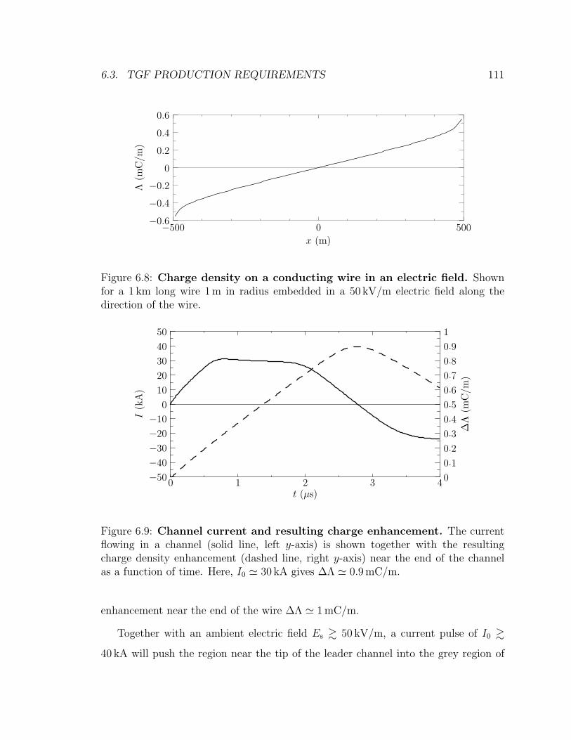
6.3. TGF PRODUCTION REQUIREMENTS 111
Figure 6.8: Charge density on a conducting wire in an electric field. Shownfor a 1 km long wire 1 m in radius embedded in a 50 kV/m electric field along thedirection of the wire.
Figure 6.9: Channel current and resulting charge enhancement. The currentflowing in a channel (solid line, left y-axis) is shown together with the resultingcharge density enhancement (dashed line, right y-axis) near the end of the channelas a function of time. Here, I0 ' 30 kA gives ∆Λ ' 0.9 mC/m.
enhancement near the end of the wire ∆Λ ' 1 mC/m.
Together with an ambient electric field Es & 50 kV/m, a current pulse of I0 &
40 kA will push the region near the tip of the leader channel into the grey region of
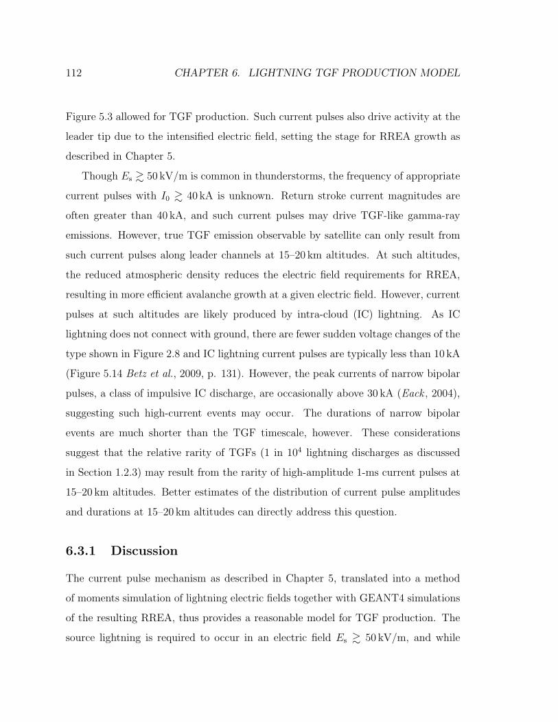
112 CHAPTER 6. LIGHTNING TGF PRODUCTION MODEL
Figure 5.3 allowed for TGF production. Such current pulses also drive activity at the
leader tip due to the intensified electric field, setting the stage for RREA growth as
described in Chapter 5.
Though Es & 50 kV/m is common in thunderstorms, the frequency of appropriate
current pulses with I0 & 40 kA is unknown. Return stroke current magnitudes are
often greater than 40 kA, and such current pulses may drive TGF-like gamma-ray
emissions. However, true TGF emission observable by satellite can only result from
such current pulses along leader channels at 15–20 km altitudes. At such altitudes,
the reduced atmospheric density reduces the electric field requirements for RREA,
resulting in more efficient avalanche growth at a given electric field. However, current
pulses at such altitudes are likely produced by intra-cloud (IC) lightning. As IC
lightning does not connect with ground, there are fewer sudden voltage changes of the
type shown in Figure 2.8 and IC lightning current pulses are typically less than 10 kA
(Figure 5.14 Betz et al., 2009, p. 131). However, the peak currents of narrow bipolar
pulses, a class of impulsive IC discharge, are occasionally above 30 kA (Eack , 2004),
suggesting such high-current events may occur. The durations of narrow bipolar
events are much shorter than the TGF timescale, however. These considerations
suggest that the relative rarity of TGFs (1 in 104 lightning discharges as discussed
in Section 1.2.3) may result from the rarity of high-amplitude 1-ms current pulses at
15–20 km altitudes. Better estimates of the distribution of current pulse amplitudes
and durations at 15–20 km altitudes can directly address this question.
6.3.1 Discussion
The current pulse mechanism as described in Chapter 5, translated into a method
of moments simulation of lightning electric fields together with GEANT4 simulations
of the resulting RREA, thus provides a reasonable model for TGF production. The
source lightning is required to occur in an electric field Es & 50 kV/m, and while
6.3. TGF PRODUCTION REQUIREMENTS 113
there is no requirement on the quantity of charge moved in the discharge, the current
pulses that stimulate leader activity, RREA seed production, and RREA must have
a magnitude of I0 & 40 kA and a duration similar to the TGF timescale. This
mechanism compares favorably with the QES and EMP TGF production mechanisms
described in Section 2.4.1 and 2.4.2 which required either extremely large charge
motions or current pulses with I0 > 400 kA.
The RREA driven by the electric field surrounding lightning leader channels as
shown in Figures 6.6 and 6.7 is emitted in a broad beam and with a spectrum char-
acteristic of RREA and bremsstrahlung as discussed in Section 3.2.1. The RREA
growth factors available in such electric fields, together with RREA seed production
by lightning leaders is sufficient to produce observable TGFs.
The model thus described therefore provides a picture of TGF production from
lightning behavior to photon emission to satellite observation. The mechanism does
not provide a complete picture, however. One limitation is the uncertainty in the
behavior of the lightning channel. In particular, the effective radius of the lightning
channel is a parameter in the current pulse simulation corresponding to the different
values of the maximum electric field considered to limit the radius of the line charges
in Chapter 5. In reality, this radius varies with time and depends on the history
of the current flowing in the channel. This dependence can significantly affect the
electric field near the channel and may also affect the behavior of current pulses on the
channel. A short review of efforts to study the behavior of the leader channel in detail
can be found in Section II of Rakov and Uman (1998). Another parameter used in the
current pulse simulation is the resistance per unit length of the channel, a parameter
that also in principle varies with time and history of the channel. Such nonlinear
resistance is easily added to the simulations described above, can affect the speed
of current pulse propagation, and may significantly complicate the overall dynamics
of the lightning discharge (De Conti et al., 2008). The effects of RREA on the

114 CHAPTER 6. LIGHTNING TGF PRODUCTION MODEL
development of the lightning channel and the behavior of the resulting electric fields
is also not treated in the model described above and may be significant, especially if
relativistic feedback is important as discussed in Section 5.5.
Chapter 7
Conclusions
This dissertation discusses a new mechanism by which terrestrial gamma-ray flashes
(TGFs) might be produced by lightning. The mechanism is arrived at as a result
first of studies of the available satellite data (Chapter 3) that indicate TGFs are
produced at 15–20 km altitudes, lower than predicted by previous mechanisms. The
low production altitude requires a total source energy of 1–10 kJ of energetic photons
as produced by bremsstrahlung from a population of 1017 electrons. In Chapter 4,
studies of the seeds available to initiate RREA give 107 as the maximum feasible
number of seed particles. The maximum avalanche multiplication factor available to
thunderstorms is roughly M = 106, thereby producing a maximum of 1013 energetic
electrons.
The discrepancy between the number of electrons that can be produced by simple
RREA of seed particles available in the thunderstorm environment and the number
required for TGF production motivates the study of TGF production by lightning
in Chapter 5. Results indicate that lightning is indeed capable of TGF production
through the action of active negative leaders. Such leaders are capable not only of
producing a large population of seed particles but also of driving RREA and ac-
celeration of these seed particles to high energies. This suggests lightning current
115
116 CHAPTER 7. CONCLUSIONS
pulse-driven TGF production, the LCP TGF production mechanism. This mecha-
nism is developed further in Chapter 6, where a model of lightning current pulses is
constructed and used to derive the properties of photon emission and the lightning
properties required to produce observable TGFs. The lightning is required to occur
in an ambient electric field of at least 50 kV/m and involve current pulses at cloud
altitude of magnitude I0 & 40 kA and duration ∼1 ms. The likelihood of such current
pulses is uncertain as intra-cloud lightning is not well-understood, but some results
indicate the requirements are not unreasonably extreme. The mechanism and model
thus put forth provide a reasonably complete picture of TGF production by lightning,
though the detailed physics of lightning discharge is not yet included in the model.
7.1 Suggestions for future work
Experimentally, new data not yet analyzed from satellites such as Fermi, AGILE,
TARANIS, and ASIM may shed new light on the physics of TGFs. Analysis of
such data as described in Chapter 3 can validate or refute the predictions made of
TGF emission by lightning in Chapter 5. Better average energy spectra and higher-
resolution energy spectra of individual TGFs can further determine the production
altitude and initial beaming of TGF photons. Correlations between TGF data and
lightning data with accurate timing, lightning geolocation, and lightning parameter
determination can provide better information not only on relative position of source
and satellite but can also help describe the properties of TGF-producing lightning.
Theoretically, the main uncertainties remaining in the physics of TGFs are the
role of relativistic feedback and the effects of RREA on the lightning discharge. Rel-
ativistic feedback can also possibly circumvent the limitations on simple avalanche
growth and seed particle populations, especially for positive leader channels. As the
effects of relativistic feedback in confined electric fields surrounding lightning and in
7.1. SUGGESTIONS FOR FUTURE WORK 117
realistic thunderstorm electric fields has not yet been well studied, examination of
relativistic feedback in the context of TGF production could be very useful. A full
model of RREA and relativistic feedback, together with the capability to model the
effects of RREA and relativistic feedback on the driving electric field, is required to
successfully address this issue. Inclusion of a model of lightning electric fields such as
the current pulse model described here would allow studies of how RREA and rela-
tivistic feedback relate to lightning discharge. Such a self-consistent model of TGFs
as may be produced by lightning and thunderstorm electric fields, with or without
relativistic feedback, would be quite valuable.
Use of the understanding gained from such studies of TGFs also provides an
opportunity to examine the implications of TGFs for atmospheric physics as a whole.
If energetic processes such as RREA are commonly associated with lightning as the
results of Chapter 5 indicate, the chemical effects could be of great interest. The
radiological implications may even be relevant as TGFs and TGF-like emissions have
been suggested to provide a significant radiation dose to a sufficiently-unlucky aircraft
(Dwyer et al., 2008b).
The lightning current pulse model described here also forms a solid basis for
future research. The detailed microphysics of the leader channel can be modeled
and included as time- and history-dependent radius and resistance parameters. The
formation and decay of the lightning channel with time can also be included by
introducing new uncharged leader channel segments or removal of existing inactive
channel segments. The resulting full time-dependent lightning model would be more
useful for lightning studies than existing time-independent fractal lightning models
(e.g., Krehbiel et al., 2008). A full time-dependent lightning model would allow for
studies of the development of intra-cloud components of lightning as well as the
resulting radio emissions and their effects such as so-called “sferic bursts” (Marshall
et al., 2007). Such a complete physically-motivated model and comparison of its

118 CHAPTER 7. CONCLUSIONS
results to observations, for instance with lightning mapping arrays, would further
overall understanding of lightning.
Bibliography
Abraham, J., et al. (2008), Correlation of the highest-energy cosmic rays with the
positions of nearby active galactic nuclei, Astroparticle Phys., 29 (3), 188–204, doi:
DOI:10.1016/j.astropartphys.2008.01.002.
Agostinelli, S., et al. (2003), G4–a simulation toolkit, Nucl. Inst. & Meth., 506 (3),
250–303.
Anthony, P. L., et al. (1997), Bremsstrahlung suppression due to the Landau-
Pomeranchuk-Migdal and dielectric effects in a variety of materials, Phys. Rev.
D, 56, 1373–1390, doi:10.1103/PhysRevD.56.1373.
Baba, Y., and V. A. Rakov (2007), Electromagnetic models of the lightning return
stroke, J. Geophys. Res., 112 (D11), D04,102, doi:10.1029/2006JD007222.
Babich, L. P., R. I. Il’kaev, I. M. Kutsyk, K. I. Bakhov, and R. A. Roussel-Dupre
(2004a), Self-consistent calculation of upward atmospheric discharge developing in
the mode relativistic runaway electron avalanches, Geomag. Aeron., 44 (2), 231–
242.
Babich, L. P., R. I. Il’kaev, I. M. Kutsyk, A. Y. Kudryavtsev, R. A. Roussel-Dupre,
and E. M. Symbalisty (2004b), Analysis of atmospheric gamma ray bursts based on
the mechanism of generation of relativistic electron avalanches, Geomag. Aeron.,
44 (2), 243–251.
119
120 BIBLIOGRAPHY
Bell, T. F., V. P. Pasko, and U. S. Inan (1995), Runaway electrons as a source of
Red Sprites in the mesosphere, Geophys. Res. Lett., 22, 2127–2130, doi:10.1029/
95GL02239.
Berger, M., J. Hubbell, S. Seltzer, J. Chang, J. Coursey, R. Sukumar, and D. Zucker
(1998), Xcom: Photon cross sections database, Tech. rep., National Institute of
Standards and Technology.
Betz, H., T. C. Marshall, M. Stolzenburg, K. Schmidt, W. P. Oettinger, E. Defer,
J. Konarski, P. Laroche, and F. Dombai (2008), Detection of in-cloud lightning with
VLF/LF and VHF networks for studies of the initial discharge phase, Geophys. Res.
Lett., 35, 23,802, doi:10.1029/2008GL035820.
Betz, H., U. Schumann, and P. Laroche (Eds.) (2009), Lightning: Principles, Instru-
ments and Applications, Springer Verlag.
Blair, T. A., and R. C. Fite (1957), Weather Elements, Prentice Hall, Englewood
Cliffs, NJ.
Carlson, B. E., N. G. Lehtinen, and U. S. Inan (2007), Constraints on terrestrial
gamma ray flash production from satellite observation, Geophys. Res. Lett., 34,
L08,809, doi:10.1029/2006GL029229.
Carlson, B. E., N. G. Lehtinen, and U. S. Inan (2008), Runaway relativistic electron
avalanche seeding in the Earth’s atmosphere, J. Geophys. Res., 113, A10,307, doi:
10.1029/2008JA013210.
Carlson, B. E., N. G. Lehtinen, and U. S. Inan (2009a), Observations of terrestrial
gamma-ray flash electrons, in COUPLING OF THUNDERSTORMS AND LIGHT-
NING DISCHARGES TO NEAR-EARTH SPACE: Proceedings of the Workshop,
BIBLIOGRAPHY 121
vol. 1118, edited by N. B. Crosby, T.-Y. Huang, and M. J. Rycroft, pp. 84–91, AIP,
doi:10.1063/1.3137717.
Carlson, B. E., N. G. Lehtinen, and U. S. Inan (2009b), Terrestrial gamma-ray flash
production by lightning current pulses, J. Geophys. Res, in press.
Carlson, B. E., et al. (2005), Search for correlated high energy cosmic ray events with
CHICOS, J. Phys. G. Nucl. Partic., 31, 409–416, doi:10.1088/0954-3899/31/5/011.
Christian, H., et al. (1999), The lightning imaging sensor, in Proceedings of the 11th
International Conference on Atmospheric Electricity, pp. 746–749, NASA.
Cohen, M. B., U. S. Inan, and G. Fishman (2006), Terrestrial gamma ray flashes ob-
served aboard the Compton Gamma Ray Observatory/Burst and Transient Source
Experiment and ELF/VLF radio atmospherics, J. Geophys. Res., 111, D24,109,
doi:10.1029/2005JD006987.
Cohen, M. B., U. S. Inan, R. K. Said, and D. M. Smith (2007), Terrestrial gamma-ray
flashes and very low frequency data, IUGG General Assembly, Perugia, Italy.
Cohen, M. B., U. S. Inan, R. K. Said, and D. M. Smith (2009), Terrestrial gamma-ray
flashes and updated very low frequency measurements, manuscript in preparation
for Geophysical Research Letters.
Coleman, L. M., and J. R. Dwyer (2006), Propagation speed of runaway electron
avalanches, Geophys. Res. Lett., 33, L11,810, doi:10.1029/2006GL025863.
Cooray, V. (2004), The lightning flash, Institution of Electrical Engineers, London.
Cummer, S. A., and U. S. Inan (2000), Modeling ELF radio atmospheric propagation
and extracting lightning currents from ELF observations, Radio Sci., 35, 385–394,
doi:10.1029/1999RS002184.
122 BIBLIOGRAPHY
Cummer, S. A., and W. A. Lyons (2004), Lightning charge moment changes in
U.S. High Plains thunderstorms, Geophys. Res. Lett., 31, 5114, doi:10.1029/
2003GL019043.
Cummer, S. A., Y. Zhai, W. Hu, D. M. Smith, L. I. Lopez, and M. A. Stanley (2005),
Measurements and implications of the relationship between lightning and terrestrial
gamma ray flashes, Geophys. Res. Lett., 32, L08,811, doi:10.1029/2005GL022778.
De Conti, A., S. Visacro, N. Theethayi, and V. Cooray (2008), A comparison of
different approaches to simulate a nonlinear channel resistance in lightning return
stroke models, J. Geophys. Res., 113 (D12), D14,129, doi:10.1029/2007JD009395.
Dwyer, J. (2003), A fundamental limit on electric fields in air, Geophys. Res. Lett.,
30 (20), 2055.
Dwyer, J., Z. Saleh, H. Rassoul, D. Concha, M. Rahman, V. Cooray, J. Jerauld,
M. Uman, and V. Rakov (2008), A study of X-ray emission from laboratory sparks
in air at atmospheric pressure, J. Geophys. Res., 113, D23,207.
Dwyer, J., et al. (2003), Energetic radiation produced during rocket-triggered light-
ning, Science, 299 (5607), 694–697.
Dwyer, J. R. (2007), Relativistic breakdown in planetary atmospheres, Phys. Plasmas,
14 (4), 042,901, doi:10.1063/1.2709652.
Dwyer, J. R. (2009), Relativistic positron/x-ray feedback and thundercloud electric
fields, AGU Chapman Conference on on the Effects of Thunderstorms and Light-
ning in the Upper Atmosphere.
Dwyer, J. R., and D. M. Smith (2005), A comparison between Monte Carlo simula-
tions of runaway breakdown and terrestrial gamma-ray flash observations, Geophys.
Res. Lett., 32, L22,804, doi:10.1029/2005GL023848.
BIBLIOGRAPHY 123
Dwyer, J. R., B. W. Grefenstette, and D. M. Smith (2008a), High-energy electron
beams launched into space by thunderstorms, Geophys. Res. Lett., 35, L02,815,
doi:10.1029/2007GL032430.
Dwyer, J. R., D. M. Smith, B. W. Grefenstette, and B. J. Hazelton (2008b), The high-
energy radiation dose received aboard aircraft exposed to a terrestrial gamma-ray
flash, AGU Fall Meeting, San Francisco.
Dwyer, J. R., et al. (2004), A ground level gamma-ray burst observed in as-
sociation with rocket-triggered lightning, Geophys. Res. Lett., 31, 5119, doi:
10.1029/2003GL018771.
Dwyer, J. R., et al. (2005), X-ray bursts associated with leader steps in cloud-to-
ground lightning, Geophys. Res. Lett., 32, 1803, doi:10.1029/2004GL021782.
Eack, K. B. (2004), Electrical characteristics of narrow bipolar events, Geophys. Res.
Lett., 31, 20,102, doi:10.1029/2004GL021117.
Eidelman, S., et al. (2004), Review of Particle Physics, Phys. Lett. B, 592, 1–1109,
doi:10.1016/j.physletb.2004.06.001.
Fishman, G. J., and C. A. Meegan (1995), Gamma-Ray Bursts, Ann. Rev. Astron.
Astrophys., 33, 415–458, doi:10.1146/annurev.aa.33.090195.002215.
Fishman, G. J., et al. (1994a), The first BATSE gamma-ray burst catalog, Astrophys.
J. Suppl., 92, 229–283, doi:10.1086/191968.
Fishman, G. J., et al. (1994b), Discovery of intense gamma-ray flashes of atmospheric
origin, Science, 264 (5163), 1313–1316.
Franz, R. C., R. J. Nemzek, and J. R. Winckler (1990), Television Image of a Large
Upward Electrical Discharge Above a Thunderstorm System, Science, 249, 48–51.
124 BIBLIOGRAPHY
Gallimberti, I., G. Bacchiega, A. Bondiou-Clergerie, and P. Lalande (2002), Fun-
damental processes in long air gap discharges, Comptes Rendus Physique, 3 (10),
1335–1359.
Goldstein, H., C. Poole, and J. Safko (2002), Classical Mechanics, Addison Wesley.
Grefenstette, B. W., D. M. Smith, J. R. Dwyer, and G. J. Fishman (2008), Time
evolution of terrestrial gamma ray flashes, Geophys. Res. Lett., 35, L06,802, doi:
10.1029/2007GL032922.
Gurevich, A., K. Zybin, and Y. Medvedev (2007), Runaway breakdown in strong
electric field as a source of terrestrial gamma flashes and gamma bursts in lightning
leader steps, Phys. Lett. A, 361 (1-2), 119–125.
Gurevich, A. V., and K. P. Zybin (2004), High energy cosmic ray particles and the
most powerful discharges in thunderstorm atmosphere, Phys. Lett. A, 329, 341–347,
doi:10.1016/j.physleta.2004.06.094.
Gurevich, A. V., G. M. Milikh, and R. A. Roussel-Dupre (1992), Runaway mechanism
of air breakdown and preconditioning during a thunderstorm, Phys. Lett. A, 165,
463–468, doi:10.1016/0375-9601(92)90348-P.
Gurevich, A. V., R. Roussel-Dupre, and K. P. Zybin (1998), Kinetic equation for
high energy electrons in gases, Phys. Lett. A, 237 (4–5), 240–246, doi:10.1016/
S0375-9601(97)00868-2.
Gurevich, A. V., L. M. Duncan, Y. V. Medvedev, and K. P. Zybin (2002), Radio emis-
sion due to simultaneous effect of runaway breakdown and extensive atmospheric
showers, Phys. Lett. A, 301, 320–326, doi:10.1016/S0375-9601(02)00900-3.
BIBLIOGRAPHY 125
Gurevich, A. V., L. M. Duncan, A. N. Karashtin, and K. P. Zybin (2003), Ra-
dio emission of lightning initiation, Phys. Lett. A, 312, 228–237, doi:10.1016/
S0375-9601(03)00511-5.
Gurevich, A. V., Y. V. Medvedev, and K. P. Zybin (2004), New type discharge
generated in thunderclouds by joint action of runaway breakdown and extensive
atmospheric shower, Phys. Lett. A, 329, 348–361, doi:10.1016/j.physleta.2004.06.
099.
Gurevich, A. V., Y. V. Medvedev, and K. P. Zybin (2004a), Thermal electrons and
electric current generated by runaway breakdown effect [rapid communication],
Phys. Lett. A, 321, 179–184, doi:10.1016/j.physleta.2003.10.062.
Gurevich, A. V., K. P. Zybin, and Y. V. Medvedev (2006), Amplification and
nonlinear modification of runaway breakdown, Phys. Lett. A, 349, 331–339, doi:
10.1016/j.physleta.2005.09.074.
Gurevich, A. V., et al. (2004b), Experimental evidence of giant electron-gamma bursts
generated by extensive atmospheric showers in thunderclouds, Phys. Lett. A, 325,
389–402, doi:10.1016/j.physleta.2004.03.074.
Hazelton, B., B. Grefenstette, D. Smith, J. Dwyer, X. Shao, S. Cummer, T. Chronis,
E. Lay, and R. Holzworth (2009), Spectral dependence of terrestrial gamma-ray
flashes on source distance, Geophys. Res. Lett., 36 (1), L01,108.
Hedin, A. E. (1991), Extension of the MSIS thermosphere model into the middle and
lower atmosphere, J. Geophys. Res., 96, 1159–1172, doi:10.1029/90JA02125.
Howard, J., M. A. Uman, J. R. Dwyer, D. Hill, C. Biagi, Z. Saleh, J. Jerauld, and
H. K. Rassoul (2008), Co-location of lightning leader x-ray and electric field change
sources, Geophys. Res. Lett., 35, 13,817, doi:10.1029/2008GL034134.
126 BIBLIOGRAPHY
Inan, U. S., and N. G. Lehtinen (2005), Production of terrestrial gamma-ray flashes
by an electromagnetic pulse from a lightning return stroke, Geophys. Res. Lett., 32,
L19,818, doi:10.1029/2005GL023702.
Inan, U. S., S. C. Reising, G. J. Fishman, and J. M. Horack (1996), On the association
of terrestrial gamma-ray bursts with lightning and implication for sprites, Geophys.
Res. Lett., 23 (9), 1017–1020, doi:10.1029/96GL00746.
Inan, U. S., M. B. Cohen, R. Said, D. M. Smith, and L. I. Lopez (2006), Terrestrial
Gamma-ray Flashes and Lightning Discharges, Geophys. Res. Lett., 33, L18,802,
doi:doi:10.1029/2006GL027085.
International Commission on Radiation Units and Measurements (1984), Stopping
powers for electrons and positrons, ICRU Rep., 37.
Jackson, J. (1999), Classical Electrodynamics, John Wiley & Sons.
Jackson, J. D. (2000), Charge density on thin straight wire, revisited, Amer. J. Phys.,
68, 789–799, doi:10.1119/1.1302908.
Jackson, J. D. (2002), Charge density on a thin straight wire: The first visit, Amer.
J. Phys., 70, 409–410, doi:10.1119/1.1432973.
Klebesadel, R. W., I. B. Strong, and R. A. Olson (1973), Observations of Gamma-Ray
Bursts of Cosmic Origin, Astrophys. J. Lett., 182, L85, doi:10.1086/181225.
Koch, H. W., and J. W. Motz (1959), Bremsstrahlung Cross-Section Formulas and
Related Data, Rev. Mod. Phys., 31, 920–955, doi:10.1103/RevModPhys.31.920.
Krehbiel, P., J. Riousset, V. Pasko, R. Thomas, W. Rison, M. Stanley, and H. Edens
(2008), Upward electrical discharges from thunderstorms, Nat. Geosci., 1 (4), 233–
237.
BIBLIOGRAPHY 127
Lee, A., E. D. Bloom, and V. Petrosian (2000), Properties of Gamma-Ray Burst Time
Profiles Using Pulse Decomposition Analysis, Astrophys. J. Suppl., 131, 1–19, doi:
10.1086/317364.
Lehtinen, N. G. (2000), Relativistic runaway electrons above thunderstorms, Ph.D.
thesis, Leland Stanford Junior University.
Lehtinen, N. G., M. Walt, U. S. Inan, T. F. Bell, and V. P. Pasko (1996), γ-ray
emission produced by a relativistic beam of runaway electrons accelerated by quasi-
electrostatic thundercloud fields, Geophys. Res. Lett., 23 (19), 2645–2648, doi:10.
1029/96GL02573.
Lehtinen, N. G., T. F. Bell, V. P. Pasko, and U. S. Inan (1997), A two-dimensional
model of runaway electron beams driven by quasi-electrostatic thundercloud fields,
Geophys. Res. Lett., 24, 2639, doi:10.1029/97GL52738.
Lehtinen, N. G., T. F. Bell, and U. S. Inan (1999), Monte Carlo simulation of runaway
MeV electron breakdown with application to red sprites and terrestrial gamma ray
flashes, J. Geophys. Res., 104 (A11), 24,699–24,712, doi:10.1029/1999JA900335.
Lehtinen, N. G., U. S. Inan, and T. F. Bell (2001), Effects of thunderstorm driven run-
away electrons in the conjugate hemisphere: Purple sprites and ionization enhance-
ments, J. Geophys. Res., 106 (A12), 28,841–28,856, doi:10.1029/2000JA000160.
Leo, W. (1994), Techniques for nuclear and particle physics experiments, 2 ed.,
Springer-Verlag, New York.
MacGorman, D. R., and W. D. Rust (1998), The Electrical Nature of Storms, Oxford
University Press, New York.
Marshall, R. A., U. S. Inan, and W. A. Lyons (2007), Very low frequency sferic bursts,
128 BIBLIOGRAPHY
sprites, and their association with lightning activity, J. Geophys. Res., 112 (D11),
22,105, doi:10.1029/2007JD008857.
Marshall, T. C., and M. Stolzenburg (2001), Voltages inside and just above thunder-
storms, J. Geophys. Res., 106 (D5), 4757–4768, doi:10.1029/2000JD900640.
Marshall, T. C., M. Stolzenburg, C. R. Maggio, L. M. Coleman, P. R. Krehbiel,
T. Hamlin, R. J. Thomas, and W. Rison (2005), Observed electric fields associated
with lightning initiation, Geophys. Res. Lett., 32, 3813, doi:10.1029/2004GL021802.
Milikh, G., and J. A. Valdivia (1999), Model of gamma ray flashes due to fractal
lightning, Geophys. Res. Lett., 26 (4), 525, doi:10.1029/1999GL900001.
Miller, E. K., A. J. Poggio, and G. J. Burke (1973), An Integro-Differential Equation
Technique for the Time-Domain Analysis of Thin Wire Structures. I. The Numerical
Method, J. Comp. Phys., 12, 24, doi:10.1016/0021-9991(73)90167-8.
Moss, G., V. Pasko, N. Liu, and G. Veronis (2006), Monte Carlo model for analysis
of thermal runaway electrons in streamer tips in transient luminous events and
streamer zones of lightning leaders, J. Geophys. Res., 111, A02,307.
Motz, J. W., H. A. Olsen, and H. W. Koch (1969), Pair Production by Photons, Rev.
Mod. Phys., 41, 581–639, doi:10.1103/RevModPhys.41.581.
Nagano, M., and A. A. Watson (2000), Observations and implications of the ultrahigh-
energy cosmic rays, Rev. Mod. Phys., 72, 689–732.
Nemiroff, R. J., J. T. Bonnell, and J. P. Norris (1997), Temporal and spectral char-
acteristics of terrestrial gamma flashes, J. Geophys. Res., 102 (A5), 9659–9666,
doi:10.1029/96JA03107.
BIBLIOGRAPHY 129
Nguyen, C. V., A. P. J. van Deursen, and U. Ebert (2008), Multiple x-ray bursts
from long discharges in air, J. Phys. D. Appl. Phys., 41 (23), 234,012, doi:10.1088/
0022-3727/41/23/234012.
Noda, T., and S. Yokoyama (2002), Thin wire representation in finite difference time
domain surge simulation, IEEE Trans. Power Deliver., 17 (3), 840–847, doi:10.
1109/TPWRD.2002.1022813.
Pasko, V. P., U. S. Inan, Y. N. Taranenko, and T. F. Bell (1995), Heating, ioniza-
tion and upward discharges in the mesosphere due to intense quasi-electrostatic
thundercloud fields, Geophys. Res. Lett., 22, 365–368, doi:10.1029/95GL00008.
Peskin, M., and D. Schroeder (1995), An introduction to quantum field theory, West-
view press.
Poggio, A. J., E. K. Miller, and G. J. Burke (1973), An Integro-Differential Equation
Technique for the Time-Domain Analysis of Thin-Wire Structures. II. Numerical
Results, J. Comp. Phys., 12, 210, doi:10.1016/S0021-9991(73)80012-9.
Rahman, M., V. Cooray, N. Ahmad, J. Nyberg, V. Rakov, and S. Sharma (2008), X
rays from 80-cm long sparks in air, Geophys. Res. Lett., 35.
Raizer, Y. P. (1997), Gas Discharge Physics, Springer.
Rakov, V., and M. Uman (1998), Review and evaluation of lightning return stroke
models including some aspects of their application, IEEE Trans. Electromagn. C.,
40 (4), 403–426.
Rakov, V., and M. Uman (2003), Lightning: Physics and Effects, Cambridge Univ.
Press, Cambridge.
Rao, S. (1999), Time domain electromagnetics, Academic Press.
130 BIBLIOGRAPHY
Rison, W., R. J. Thomas, P. R. Krehbiel, T. Hamlin, and J. Harlin (1999), A GPS-
based three-dimensional lightning mapping system: Initial observations in central
New Mexico, Geophys. Res. Lett., 26, 3573–3576, doi:10.1029/1999GL010856.
Roussel-Dupre, R. A., A. V. Gurevich, T. Tunnel, and G. M. Milikh (1994), Kinetic
theory of runaway breakdown, Phys. Rev. E, 49, 2257–2271, doi:0.1103/PhysRevE.
49.2257.
Ruina, J., L. Alvarez, W. Donn, R. Garwin, R. Giacconi, R. Muller, W. Panofsky,
A. Peterson, and F. W. Sarles (1980), Ad hoc panel on the september 22 event,
Tech. rep., Office of Science and Technology Policy, available at http://www.gwu.
edu/~nsarchiv/NSAEBB/NSAEBB190/09.pdf.
Said, R. (2009), Accurate and efficient long-range lightning geo-location using a vlf
radio atmospheric waveform bank, Ph.D. thesis, Leland Stanford Junior University.
Sciutto, S. J. (2002), AIRES User’s Manual and Reference Guide, version 2.6.0,
available online at http://www.fisica.unlp.edu.ar/auger/aires/.
Smith, D. M. (2006), personal communication.
Smith, D. M. (2009), personal communication.
Smith, D. M., L. I. Lopez, R. P. Lin, and C. P. Barrington-Leigh (2005), Terrestrial
gamma flashes observed up to 20 MeV, Science, 307 (5712), 1085–1088, doi:10.
1126/science.1107466.
Smith, D. M., J. R. Dwyer, B. W. Grefenstette, B. J. Hazelton, Y. Yair, J. Bor, E. H.
Lay, and R. H. Holzworth (2007), Unusual RHESSI TGFs: electron beams and
others, AGU Fall Meeting, San Francisco.
BIBLIOGRAPHY 131
Smith, P. (1990), Instabilities in time marching methods for scattering: Cause and
rectification, Electromagnetics, 10 (4), 439–451.
Sokolsky, P. (1989), Introduction to Ultrahigh Energy Cosmic Ray Physics, Addison-
Wesley, New York.
Stanley, M. A., X.-M. Shao, D. M. Smith, L. I. Lopez, M. B. Pongratz, J. D. Harlin,
M. Stock, and A. Regan (2006), A link between terrestrial gamma-ray flashes and
intracloud lightning discharges, Geophys. Res. Lett., 33, L06,803.
Stolzenburg, M., and T. C. Marshall (2008), Charge Structure and Dynamics in
Thunderstorms, Space Sci. Rev., 137, 355–372, doi:10.1007/s11214-008-9338-z.
Symbalisty, E. M. D., R. A. Roussel-Dupre, and V. A. Yukhimuk (1998), Finite
volume solution of the relativistic Boltzmann equation for electron avalanche rates,
IEEE Trans. Plasma Sci., 26 (5), 1575–1582, doi:10.1109/27.736065.
Thomas, R. J., P. R. Krehbiel, W. Rison, T. Hamlin, J. Harlin, and D. Shown (2001),
Observations of VHF source powers radiated by lightning, Geophys. Res. Lett., 28,
143–146, doi:10.1029/2000GL011464.
Williams, E., et al. (2006), Lightning flashes conducive to the production and escape
of gamma radiation to space, J. Geophys. Res., 111, D16,209.
Wilson, C. T. R. (1924), The electric field of a thundercloud and some of its effects,
Proc. Roy. Soc. London, 37, 32D–37D.
Wolfendale, A. W. (Ed.) (1973), Cosmic rays at ground level, Institute of Physics,
London.
Wood, T. G. (2004), Geo-location of individual lightning discharges using impulsive
VLF electromagnetic waveforms, Ph.D. thesis, Leland Stanford Junior University.
132 BIBLIOGRAPHY
Wood, T. G., and U. S. Inan (2002), Long-range tracking of thunderstorms using
sferic measurements, J. Geophys. Res., 107, 4553, doi:10.1029/2001JD002008.
Yair, Y. (2008), Charge Generation and Separation Processes, Space Sci. Rev., 137,
119–131, doi:10.1007/s11214-008-9348-x.
Related Documents


![TERRESTRIAL GAMMA-RAY FLASHES · the satellite-detected gamma rays. 4. Gamma Ray Survival From Thunderstorm to Satellite [20] The interaction of gamma rays with atmospheric air and](https://static.cupdf.com/doc/110x72/5ca8857e88c993e47d8bc64f/terrestrial-gamma-ray-flashes-the-satellite-detected-gamma-rays-4-gamma-ray.jpg)
